The Cost of Keeping Track

Johannes Haushofer∗

August 9, 2014

Abstract

I show that a lump-sum cost incurred for keeping track of future transactions predicts severalknown departures from the standard discounting model: an agent who incurs such costs willexhibit decreasing impatience with preference reversals; a magnitude effect, i.e. discountinglarge amounts less than small amounts; a sign effect, i.e. discounting gains more than losses;and an Andreoni-Sprenger (2012) type reduction of discounting and decreasing impatience whendelayed outcomes are added onto existing delayed outcomes. In addition, agents of this type willunder certain circumstances prefer to “pre-crastinate”, i.e. incur losses sooner rather than later,which is a common feature of everyday experience but is currently not captured in discountingmodels. Additionally, the model generates loss aversion, one of the hallmarks of prospect theory.Finally, the model predicts status quo bias and default choice. In particular, it predicts thatagents will fail to adopt profitable technologies, not because they do not value them, but becausethey forget to undertake the steps necessary to use them. The model further predicts that thisproblem can be alleviated through reminders, for which agents are willing to pay. Examples indevelopment economics include SMS reminders to save, chlorine dispensers at the water source,vaccination camps, and reminders to use fertilizer.

∗Department of Psychology, Department of Economics, and Woodrow Wilson School of Public and InternationalAffairs, Princeton University, Princeton, NJ. I thank Ben Golub, Pam Jakiela, and Jeremy Shapiro for comments,and Allan Hsiao for excellent research assistance.

1

1 Introduction

Individuals often have to keep track of future transactions. For instance, when a person makes adecision to pay a bill not now, but later, she has to keep this in mind and perform an action laterto implement the decision (e.g. logging into her online bank account and making the transfer). Ifshe fails to make the transfer, she may face a late fee. Similarly, when she expects a payment, sheis likely to keep track of the incoming payment by verifying whether it arrived in her bank account.If she fails to keep track of the incoming payment, it may get lost and she may have to pay a hasslecost to follow up on it.

The basic premise of this paper is that such “keeping track” generates costs for the agent. This costcan come in several forms: agents may forget about the future transaction, resulting in a penaltysuch as a late fee, or a hassle cost to salvage the transaction. Additionally, simply having to keepthe task in mind may generate a psychological cost; this cost may be avoidable through reminders,but these in turn may be costly to set up. In either case, the agent integrates into her decisiontoday the cost of keeping track of future transactions.

This simple addition to the standard model turns out to predict several anomalies of time discountingthat the literature has documented: decreasing impatience and preference reversals; the magnitudeeffect; the sign effect; and a reduction of discounting and hyperbolicity when delayed outcomes areadded to existing delayed outcomes. In addition, the model explains why individuals under somecircumstances prefer to “pre-crastinate”, i.e. “get painful transactions over with”. This phenomenonhas recently been empirically demonstrated (Rosenbaum et al., 2014), but is not captured by existingdiscounting models. Moreover, the model predicts loss aversion for future outcomes: both futuregains and losses are less attractive due to the cost of keeping track, which decreases the utility offuture gains but increases the disutility of future losses, leading to loss aversion.

The particular form of the cost of keeping track matters for some of these results, but not for others.In particular, when the cost of keeping track is lump-sum, agents will exhibit decreasing impatienceand preference reversals in discounting, the magnitude effect, and the Andreoni-Sprenger (2012)type reduction of discounting and decreasing impatience when delayed outcomes are added ontoexisting delayed outcomes. A lump-sum cost of keeping track is realistic in cases where penaltiesfor forgetting about everyday transactions come in lump-sum form. For instance, communicationscompanies and banks frequently impose lump-sum penalties for late bill payment. In contrast,the sign effect, “pre-crastination”, loss aversion for future outcomes, and status quo bias and defaultchoice can be produced without the lump-sum assumption. Section 2.3 discusses different functionalforms for the cost of keeping track.

Finally, the model predicts status quo bias and default choice, and in particular that agents willfail to adopt profitable technologies. Lack of demand for profitable technologies is a commonphenomenon especially in developing countries. The model suggests one possible reason for thisinefficiency: when people face an opportunity to adopt technology, they often cannot act on it

2

immediately, but instead have to make a plan to do it later. For instance, when people fetch waterat a source, they might be reminded that they want to chlorinate their water. However, whenopportunities to chlorinate are not available at the source, they have to make a plan to do it later,e.g. when they reach their home where they store their chlorine bottle. However, at the latertimepoint when they can act on their plan, they have forgotten about it – in this example, bythe time they reach the homestead, they do not remember to use the chlorine bottle. The modelcaptures this phenomenon, and predicts that when reminders are provided at the right time – e.g.,at the water source – adoption should be high. Indeed, Kremer et al. (2009) show that dispensers atthe water source can dramatically increase takeup. Other authors have documented similar failuresto adopt technology, and shown that reminders at the right time – i.e., when people can act onthem – can increase takeup: timed discounts after the harvest can increase fertilizer usage amongfarmers (Duflo et al., 2009), vaccination camps and small gifts can increase vaccination rates forchildren (Banerjee et al., 2010), and text message reminders can increase savings rates (Karlan etal., 2010). The model makes quantitative predictions about the willingness of sophisticates to payfor such reminders.

The remainder of the paper is organized as follows. Section 2 presents a simple version of the modelin which utility is linear and the cost of keeping track is constant and lump-sum. Section 3 dicussesa number of alternative formulations for the shape of the cost of keeping track. Section 4 shows thatmost results hold for any concave and monotonically increasing utility function. Section 5 describesa few applications of the model in the developing world. Section 6 concludes.

2 The Model

2.1 A two-period model

We begin with a simple two-period model in which “tasks” and “opportunities” arise at the beginningof period 0. A task is a payment to be made; an opportunity is a payment to be received. Whena task or opportunity arises, the agent either decides to act on it in period 0, or to act on it inperiod 1. Acting on a task or opportunity consists in performing a costless action a. For instance,in the case of paying a bill, acting on the task consists in making the required bank transfer orwriting a check; in the case of receiving a payment, acting on the opportunity might consist in firstsending one’s bank details to the sender and verifying that the payment has arrived. Each task oropportunity is defined by the payoff of acting on it immediately, x0, and the payoff of acting on itlater, x1, with x1 ≥ x0. These payoffs accrue in the period in which the agent acts on the task oropportunity.1

1This assumption is important for the results that follow, but it is not obvious and bears justification. Specifically,under the permanent income hypothesis, agents integrate the anticipated gain or loss into their consumption pathas soon as it is announced, and they adjust consumption immediately following the anncouncement. In contrast, thepresent setup assumes that agents actually experience a (possibly transient) increase or decrease in consumption (or

3

The core assumption of the model is that when an agent decides to act on a task or opportunity inperiod 1, she incurs a cost c. I begin by modeling this cost as a lump-sum cost; Section 3 extends theframwork to other formulations. Similarly, I begin by using linear utility; this choice is motivatedby the fact that for the relatively small magnitude of the transactions which this model concerns,linear utility is a reasonable approximation. Section 4 provides a more general treatment.

Gains I now ask how agents behave when they are presented with an opportunity on whichthey can act now or later. For instance, they may receive a check in the mail which they cancash immediately or later; they may decide between selling stock now or later; or in an analogousexperiment, they may face a choice between a smaller amount available sooner or a larger amountavailable later.

The utility of acting in period 0 is:

u+0 = x0 (1)

The utility of acting in period 1 is:u+

1 = β (x1 − c) (2)

Thus, for acting in period 1, agents anticipate the discounted period 1 payoff, x1, less the discountedcost of keeping track of the opportunity. The condition for preferring to act in period 1 is u1 > u0,which simplifies to:

x1 >x0

β+ c (3)

Thus, agents prefer to act in period 1 if the future gain exceeds the future-inflated value of thesmall-soon gain and the cost of keeping track.

Losses I now extend this framework to losses, by asking how agents behave when they are pre-sented with a task which they can complete now or later. For instance, they may receive a bill inthe mail which they can pay immediately or later; farmers may decide between buying fertilizernow or later; or participants in an experiment may face a choice between losing a smaller amountof money immediately, or losing a larger amount later. To preserve the analogy to the frameworkfor gains, I consider the utility of a smaller loss −x0 incurred in period 0, and that of a larger loss−x1 incurred in period 1. If they choose the larger loss in period 1, agents additionally pay the costof keeping track. The utilities are thus as follows:

utility) in the period when they actually incur the gain or loss. Which of these competing claims is true? Empiricalevidence sides with the latter; a large number of studies show that consumption smoothing in real life is imperfect, i.e.people consume somewhat less in periods in which they incur losses (“lean season”), and somewhat more in periodsin which they incur gains (payday effects).

4

u−0 = −x0 (4)

u−1 = β (−x1 − c) (5)

The condition for acting in period 1 is again given by u1 > u0, which simplifies to:

x1 <x0

β− c (6)

Thus, agents prefer to delay losses if the future loss −x1 is sufficiently small relative to the immediateloss net of the cost of keeping track.

I now discuss the implications of this framework for choice behavior.

Proposition 1. Steeper discounting of gains: With a positive cost of keeping track, agents discountfuture gains more steeply than otherwise.

Proof. From 2, it is easy to see that ∂u+1

∂c = −β. Thus, the discounted value of future gains decreasesin the cost of keeping track, c; agents discount future gains more steeply the larger the cost of keepingtrack.

One implication of this result is that agents discount future outcomes at a higher rate than givenby their time preference parameter. For instance, even agents who discount at the interest rate willexhibit choice behavior that looks like much stronger discounting when the cost of keeping trackis high. The high discount rates frequently observed in experiments may partly be accounted forby participants correctly anticipating the cost of keeping track of the payment. For instance, ina standard discounting experiment, participants may be given a voucher to be cashed in in thefuture; with a positive probability of losing these vouchers, or of automatic payments not arriving,the future will be discounted more steeply than otherwise.

Proposition 2. Shallower discounting of losses: With a positive cost of keeping track, agents dis-count future losses less steeply than otherwise.

Proof. As above, it follows from 5 that ∂u−1∂c = −β. Thus, the discounted utility of future losses

decreases in the cost of keeping track, c; put differently, the disutility of future losses increases inc, i.e. future losses are discounted less as the cost of keeping track rises.

Intuitively, both delayed losses and delayed gains become less attractive because of the penalty forforgetting, which corresponds to steepr discounting for gains and shallower discounting for losses.

Proposition 3. Pre-crastination: When agents choose between an equal-sized immediate vs. delayedloss, they prefer to act in period 1 when the cost of keeping track is zero, but may prefer to “pre-crastinate” if with a positive cost of keeping track.

5

Proof. When the payoffs of acting now vs. acting later are both −x̄, and c = 0, the condition foracting later on losses given in Equation 6 simplifies to x̄ < x̄

β , which is always true with β < 1.Thus, when agents choose between equal-sized immediate vs. delayed losses and c = 0, they preferto act in period 1. However, when c > 0, agents may prefer to act in period 0: the condition foracting in period 0 implied by 4 and 5 is −x̄ > β (−x̄− c), which simplifies to

c >1− ββ

x̄

When this condition is met, i.e. the cost of keeping track of having to act later is large enough,agents prefer to incur the loss in period 0 rather than period 1, i.e. they “pre-crastinate”.

Under standard discounting, agents want to delay losses: a loss is less costly when it is incurred inthe future compared to today. However, if the risk and penalty for forgetting to act in period 1 aresufficiently large relative to the payoff, agents prefer to act in period 0, i.e. they “pre-crastinate”.For instance, such individuals may prefer to pay bills immediately because making a plan to paythem later is costly. This phenomenon corresponds well to everyday experience, and has recentlybeen empirically demonstrated (Rosenbaum et al., 2014). However, it is not captured by standarddiscounting models, under which agents weakly prefer to delay losses.

Proposition 4. Sign effect: With a positive cost of keeping track, agents discount gains more thanlosses.

Proof. I show that the absolute value of the utility of a delayed loss is greater than that of a delayedgain, which corresponds to greater discounting of gains than losses. The absolute value of the utilityof a delayed loss is

| u−1 |=| β (−x1 − c) |= β(x1 + c)

Because u+1 = β(x1 − c), it is easy to see that | u−1 |> u+

1 .

This result produces a the sign effect, a well-known departure of empirically observed time prefer-ences from standard discounting models: agents discount losses less than gains.

Proposition 5. Loss aversion: With a positive cost of keeping track, agents exhibit loss aversionfor future outcomes.

Proof. Follows directly from Proposition 4.

Proposition 6. Magnitude effect: With a positive cost of keeping track, agents discount largeamounts less than small amounts.

Proof. Consider the utilities of acting now vs. later when both payoffs are multiplied by a constantA > 1:

6

u0 = Ax0

u1 = β(Ax1 − c)

The condition for acting in period 1 is now:

x1 >x0

β+c

A

Recall that the condition for acting on gains in period 1 with c > 0 is x1 >x0β + c. Because c

A < c,the condition for acting in period 1 is easier to meet when the two outcomes are larger; thus, largeoutcomes are discounted less than small ones. Note that this model predicts no magnitude effectwhen both outcomes are in the future.

Proposition 7. Decreasing impatience and preference reversals: With a positive cost of keepingtrack, agents exhibit decreasing impatience and time-inconsistent preference reversals.

Proof. When both outcomes are moved one period into the future, they are both subject to the riskand penalty of forgetting; their utilities are:

u1 = β(x0 − c)

u2 = β2(x1 − c)

The condition for acting later isx1 >

x0

β

Note that this condition is easier to meet than condition 3 for choosing between acting immediatelyvs. next period, which is x1 >

x0β + c. Thus, when both outcomes are delayed into the future, the

cost of waiting is smaller. As the future approaches, this will produce the preference reversals, awell-known empirical fact about discounting.

Proposition 8. Andreoni-Sprenger convex budgets, Effect 1: With a positive cost of keeping track,agents exhibit less discounting when adding money to existing payoffs than otherwise.

Proof. Assume a fixed initial payoff x̄ in both periods 0 and 1. The lifetime utility of the agent inthe absence of other transfers is

U(x̄, x̄) = x̄+ β(x̄− c)

7

Now consider how this utility changes after adding x0 in period 0 or x1 in period 1:

U (x̄+ x0, x̄) = x̄+ x0 + β(x̄− c)

U(x̄, x̄+ x1) = x̄+ β(x̄+ x1 − c)

The condition for acting later is U(x̄, x̄+ x1) > U(x̄+ x0, x̄), which simplifies to

x1 >x0

β

Note that this condition is again easier to meet than than condition 3 for choosing between actingimmediately vs. next period without pre-existing payoffs at these timepoints. Thus, agents exhibitless discounting when money is added to existing payoffs than otherwise.

In their study on estimating time preferences from convex budgets, Andreoni & Sprenger (2012) paythe show-up fee of $10 in two instalments: $5 on the day of the experiment, and $5 later. Even thepayment on the day of the experiment is delivered to the student’s mailbox rather than given at thetime of the experiment itself, thus holding the cost of keeping track constant. The additional costof payments now vs. later is thus minimal. Andreoni & Sprenger (2012) find much lower discountrates than most other studies on discounting. This finding is reflected in the result above.

Proposition 9. Andreoni-Sprenger convex budgets, Effect 2: With a positive cost of keeping track,agents exhibit no hyperbolic discounting when adding money to existing payoffs.

Proof. Assume again a fixed initial payoff x̄ in both periods, but now move these periods one periodinto the future. The lifetime utility of the agent is

U = β(x̄− c) + β2(x̄− c)

Now consider how this utility changes after adding x0 in period 1, or x1 in period 2:

U(0, x̄+ x0, x̄) = β(x̄+ x0 − c) + β2(x̄− c)

U(0, x̄, x̄+ x1) = β(x̄− c) + β2(x̄+ x1 − c)

The condition for acting later, U(0, x̄, x̄+ x1) > U(0, x̄+ x0, x̄), simplifies to

x1 >x0

β

8

Note that this condition is the same as that obtained in Propostion 8. Thus, when money is added toexisting payoffs now vs. next period, and when money is added to existing payoffs in two consecutiveperiods in the future, the conditions for preferring to act later are the same. This model thereforeproduces no decreasing impatience or preference reversals when adding money to existing payoffs.This mirrors the second result in Andreoni & Sprenger’s (2012) study.

Together, these results predict many of the anomalies that characterize empirically obtained dis-count functions. Figure 1 summarizes the magnitude and sign effects and hyperbolic discountinggraphically.

3 Anatomy of the cost of keeping track

In the previous section, the cost of keeping track was a lump-sum to simplify exposition. In thissection I consider a few variations. The key result is that most of the results above hold for differentformulations of the cost of keeping track.

3.1 The risk of forgetting

Perhaps the most compelling argument in support of the assumption that agents incur a cost forkeeping track of future transactions is the fallibility of human memory. If agents are more likelyto forget acting on future transactions than current transactions, this naturally leads to the resultsderived in the previous sections. Specifically, assume that when an agent makes a plan to act ona task or opportunity in the future, she actually performs the required action with probability1 − p < 1, and forgets to perform the action with probability p > 0. If she forgets to perform theaction required to act on the task or opportunity, the agent receives a smaller payoff xD < x1; inthe case of losses, she incurs a greater loss, −xD < −x1. We can think of the difference between xDand x1 as the penalty c for forgetting to act, with c = x1 − xD > 0 for gains and c = xD − x1 > 0

for losses. For instance, the agent can still cash a check that she forgot to cash by the deadline, butincurs a cost to “salvage” the transaction, e.g. by paying an administrative fee to have a new checkissued. Similarly, if the agent fails to pay a bill by the deadline, the bill will still be paid, but theagent now has to pay a late fee. Thus, the utility for gains is now as follows:

u+1 = β [(1− p)x1 + pxD]

With the penalty for forgetting given by c = x1 − xD > 0, this simplifies to:

u+1 = β (x1 − pc)

Similarly, the utility for losses is:

9

u−1 = β [(1− p)(−x1) + p(−xD)]

With the penalty for forgetting given by c = xD − x1 > 0, this simplifies to:

u−1 = β [−x1 − pc]

Note that both of these utilities are variants of the utilities obtained with a lump-sum cost ofkeeping track in 2 and 5; here, the cost c is additionally multiplied with the probability that it willbe incurred. Because both p and c are constant for all future periods, this formulation yields thesame results as those in section 2.1.

3.1.1 The shape of the forgetting function

From the previous discussion, naturally the question arises whether a constant probability of for-getting for all future periods is justified. Indeed, this particular choice is motivated by the currentconsensus in psychology about the empirical shape of the forgetting function: as was first casuallyobserved by the German psychologist Jost in 1897, and confirmed by Wixted and colleagues (e.g.Wixted, 2004) and many other studies since, the shape of the psychological forgetting function isnot well described by an exponential function, but follows instead a power law, such as a hyper-bola. Note that a fixed probability of forgetting attached to future but not present transactionsis a quasi-hyperbolic forgetting function similar to that used for discounting by Strotz (1956) andLaibson (1997). This assumption generates decreasing impatience and preference reversals.

3.1.2 Beyond forgetting: reminders and hassle costs

Having imperfect memory might not be a problem if agents anticipate their own probability offorgetting to act in the future (as we have assumed so far), and can set up costless reminders toovercome this risk. However, I argue that truly effective reminders are unlikely to be costless.First, even the small act of making a note in one’s diary about the future task or opportunity arehassle costs that can be cumbersome. Second, such simple reminders are not bullet-proof, and trulyeffective reminders are likely to be much more costly. For instance, consider the actions you wouldhave to undertake to avoid forgetting an important birthday with a probability of one. Writing itin a diary is not sufficient because you might forget to look at it. Setting an alarm, e.g. on a phone,might fail because the phone might be out of battery at the wrong time. A personal assistant mightforget himself to issue the reminder to you. Likely the most effective way of ensuring that thebirthday is not forgotten would be to hire a personal assistant whose sole assignment is to issue thereminder. Needless to say, this would be rather costly. Cheaper versions of the same arrangementwould come at the cost of lower probabilities of the reminder being effective.

10

Finally, even if agents have perfect memory, they may incur a psychological cost for keeping trans-actions in mind. The psychological cost of juggling many different tasks has recently attractedincreased interest in psychology and economics. Most prominently, Shafir & Mullainathan (2013)argue that the poor in particular may have so many things on their mind that only the most press-ing receive their full attention. This argument implies that a) allocating attention to a task is notcostless, and b) the marginal cost of attention is increasing in the number of tasks. Together, thisreasoning provides an intuition for a positive psychological cost of keeping track of future transac-tions, even with perfect memory and no financial costs of keeping track.

3.2 A proportional cost of keeping track

In the previous exposition, the cost of keeping track was a lump-sum cost that was subtracted fromfuture payoffs. In this section, I ask how the results obatined with a lump-sum cost would changeif the cost were instead a fraction α of the original payoff. The utility of gains is then given by:

u+1 = β(1− α)x1 (7)

Analogously, the utility for losses is given by:

u−1 = β(1 + α)(−x1) (8)

The condition for choosing the larger, later gain is

x1 >x0

β(1− α)(9)

Analogously, the condition for choosing the larger, later loss is

x1 <x0

β(1 + α)(10)

Note that in the gains domain, this formulation for the cost of keeping track creates the quasi-hyperbolic discounting model (Strotz, 1956; Laibson, 1996), which measures exponential period-by-period discounting through the parameter δ, which corresponds to β in the present model, andhyperbolicity through the β parameter which is multiplied onto any future outcome; this parametercorresponds to (1 − α) in the present model. Thus, in the gains domain, the present model witha cost of keeping track model that is a fraction of the original payoff generates the same results asthe quasi-hyperbolic discounting model.

11

Specifically, with a positive cost of keeping track, agents discount more than they would otherwise;it is easy to see from equation7 that ∂u+

1∂α < 0. Thus, Proposition 1 continues to hold with a

proportional cost of keeping track. Moreover, because the same proportional cost applies to allfuture transactions, but not present transactions, the model with a proportional cost of keepingtrack generates decreasing impatience. Consider the utilities if the choice between x0 immediatelyand x1 next period is moved one period into the future. The period 1 utility is then given by

u+1 = β(1− α)x0

and the period 2 utility is given by

u+2 = β2(1− α)x1

The condition for choosing the larger, later outcome is

x1 >x0

β

Note that this condition is easier to meet than condition 9; thus, agents exhibit decreasing impa-tience, and Proposition 7 therefore continues to hold. Thus, in the gains domain, the model with aproportional cost coincides with the quasi-hyperbolic discounting model and makes the same corepredictions.

However, the two models differ in the loss domain: while the quasi-hyperbolic model discountsboth gains and losses with the same parameters, in the present model, the cost-of-keeping-trackparameter is 1 + α for losses (since a larger loss is incurred when agents fail to keep track of thetransaction), while it is 1 − α for gains (since a smaller gain is obtained when agents fail to keeptrack). As a result, the present model predicts the sign effect in discounting, loss aversion for futuretransactions, and pre-crastination.

To see the sign effect, compare the absolute value of a delayed loss to that of a delayed gain:

| u−1 |=| β(1 + α)(−x1) |= β(1 + α)x1 > β(1− α)x1 = u+1

Thus, the absolute value of the utility of a delayed loss is greater than that of a delayed gain, whichimplies greater discounting of gains than losses. This result corrresponds to that of Proposition 4above. By the same reasoning, loss aversion for delayed outcomes (Proposition 5) continues to holdwith a proportional cost of keeping track.

To see that agents may prefer to pre-crastinate with a proportional cost of keeping track, considerthe case where the payoffs of acting now vs. acting later are both −x̄. When α = 0, the conditionfor acting later on losses given in Equation 10 simplifies to x̄ < x̄

β , which is always true with β < 1.

12

Thus, when agents choose between equal-sized immediate vs. delayed losses and α = 0, they preferto act in period 1. However, when α > 0, agents may prefer to act in period 0: the condition foracting in period 0 implied by 4 and 8 is

−x̄ > β(1 + α) (−x̄)

which simplifies to

α >1− ββ

Thus, when the proportional cost of keeping track is sufficiently high relative to the cost of waiting,agents prefer to pre-crastinate.

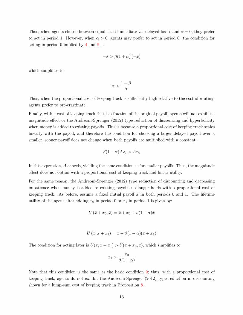
Finally, with a cost of keeping track that is a fraction of the original payoff, agents will not exhibit amagnitude effect or the Andreoni-Sprenger (2012) type reduction of discounting and hyperbolicitywhen money is added to existing payoffs. This is because a proportional cost of keeping track scaleslinearly with the payoff, and therefore the condition for choosing a larger delayed payoff over asmaller, sooner payoff does not change when both payoffs are multiplied with a constant:

β(1− α)Ax1 > Ax0

In this expression, A cancels, yielding the same condition as for smaller payoffs. Thus, the magnitudeeffect does not obtain with a proportional cost of keeping track and linear utility.

For the same reason, the Andreoni-Sprenger (2012) type reduction of discounting and decreasingimpatience when money is added to existing payoffs no longer holds with a proportional cost ofkeeping track. As before, assume a fixed initial payoff x̄ in both periods 0 and 1. The lifetimeutility of the agent after adding x0 in period 0 or x1 in period 1 is given by:

U (x̄+ x0, x̄) = x̄+ x0 + β(1− α)x̄

U (x̄, x̄+ x1) = x̄+ β(1− α)(x̄+ x1)

The condition for acting later is U(x̄, x̄+ x1) > U(x̄+ x0, x̄), which simplifies to

x1 >x0

β(1− α)

Note that this condition is the same as the basic condition 9; thus, with a proportional cost ofkeeping track, agents do not exhibit the Andreoni-Sprenger (2012) type reduction in discountingshown for a lump-sum cost of keeping track in Proposition 8.

13

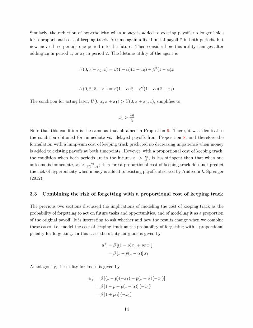
Similarly, the reduction of hyperbolicity when money is added to existing payoffs no longer holdsfor a proportional cost of keeping track. Assume again a fixed initial payoff x̄ in both periods, butnow move these periods one period into the future. Then consider how this utility changes afteradding x0 in period 1, or x1 in period 2. The lifetime utility of the agent is

U(0, x̄+ x0, x̄) = β(1− α)(x̄+ x0) + β2(1− α)x̄

U(0, x̄, x̄+ x1) = β(1− α)x̄+ β2(1− α)(x̄+ x1)

The condition for acting later, U(0, x̄, x̄+ x1) > U(0, x̄+ x0, x̄), simplifies to

x1 >x0

β

Note that this condition is the same as that obtained in Propostion 9. There, it was identical tothe condition obtained for immediate vs. delayed payoffs from Proposition 8, and therefore theformulation with a lump-sum cost of keeping track predicted no decreasing impatience when moneyis added to existing payoffs at both timepoints. However, with a proportional cost of keeping track,the condition when both periods are in the future, x1 >

x0β , is less stringent than that when one

outcome is immediate, x1 >x0

β(1−α) ; therefore a proportional cost of keeping track does not predictthe lack of hyperbolicity when money is added to existing payoffs observed by Andreoni & Sprenger(2012).

3.3 Combining the risk of forgetting with a proportional cost of keeping track

The previous two sections discussed the implications of modeling the cost of keeping track as theprobability of forgetting to act on future tasks and opportunities, and of modeling it as a proportionof the original payoff. It is interesting to ask whether and how the results change when we combinethese cases, i.e. model the cost of keeping track as the probability of forgetting with a proportionalpenalty for forgetting. In this case, the utility for gains is given by

u+1 = β [(1− p)x1 + pαx1]

= β [1− p(1− α)]x1

Anaologously, the utility for losses is given by

u−1 = β [(1− p)(−x1) + p(1 + α)(−x1)]

= β [1− p+ p(1 + α)] (−x1)

= β [1 + pα] (−x1)

14

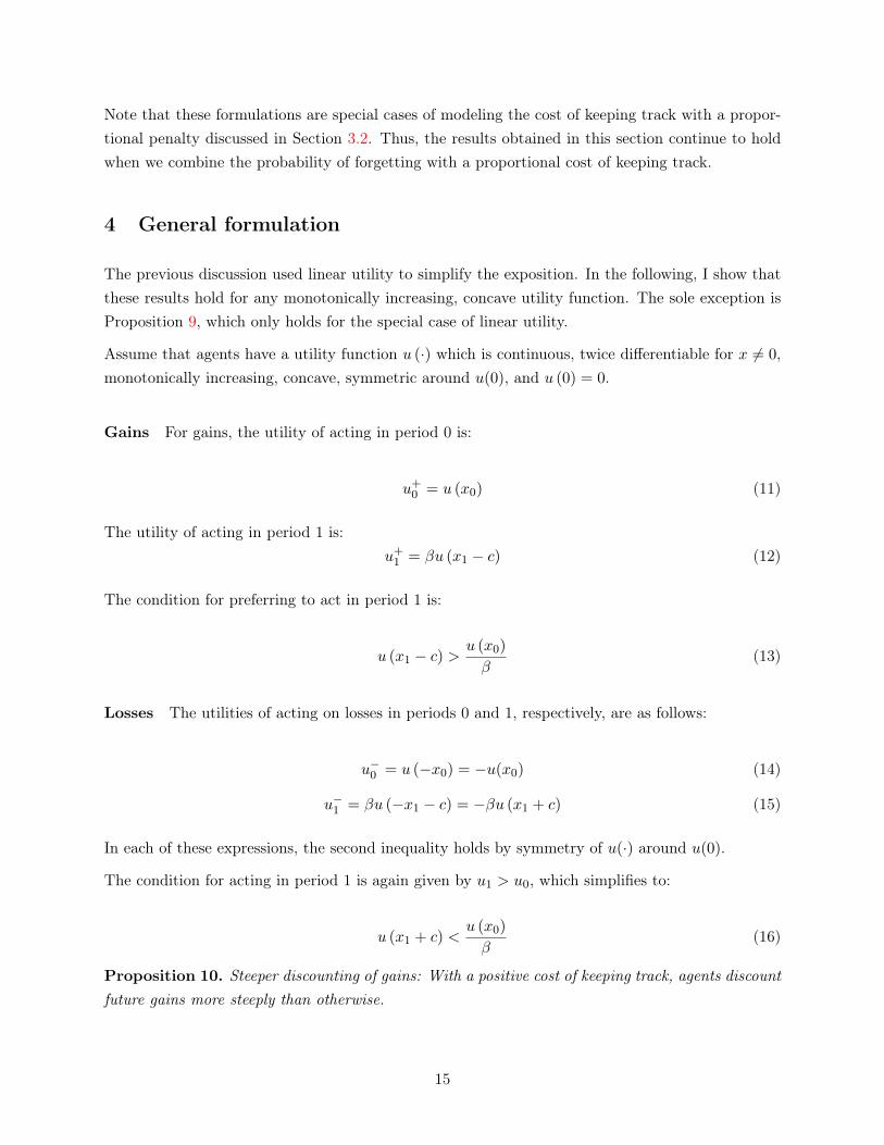
Note that these formulations are special cases of modeling the cost of keeping track with a propor-tional penalty discussed in Section 3.2. Thus, the results obtained in this section continue to holdwhen we combine the probability of forgetting with a proportional cost of keeping track.

4 General formulation

The previous discussion used linear utility to simplify the exposition. In the following, I show thatthese results hold for any monotonically increasing, concave utility function. The sole exception isProposition 9, which only holds for the special case of linear utility.

Assume that agents have a utility function u (·) which is continuous, twice differentiable for x 6= 0,monotonically increasing, concave, symmetric around u(0), and u (0) = 0.

Gains For gains, the utility of acting in period 0 is:

u+0 = u (x0) (11)

The utility of acting in period 1 is:u+

1 = βu (x1 − c) (12)

The condition for preferring to act in period 1 is:

u (x1 − c) >u (x0)

β(13)

Losses The utilities of acting on losses in periods 0 and 1, respectively, are as follows:

u−0 = u (−x0) = −u(x0) (14)

u−1 = βu (−x1 − c) = −βu (x1 + c) (15)

In each of these expressions, the second inequality holds by symmetry of u(·) around u(0).

The condition for acting in period 1 is again given by u1 > u0, which simplifies to:

u (x1 + c) <u (x0)

β(16)

Proposition 10. Steeper discounting of gains: With a positive cost of keeping track, agents discountfuture gains more steeply than otherwise.

15

1. Cost is lump sum 2. Cost is fraction of original payoffImmediate utility (gains) u+

0 = x0 u+0 = x0

Immediate utility (losses) u−0 = −x0 u−0 = −x0

Delayed utility (gains) u+1 = β(x1 − c) u+

1 = β(1− α)x1

Delayed utility (losses) u−1 = β(−x1 − c) u−1 = β(1 + α)(−x1)

Basic condition (gains) x1 >x0β + c x1 >

x0β(1−α)

1. More discounting of gains Yes Yes∂u+

1∂c < 0

∂u+1

∂α < 0

2. Less discounting of losses Yes Yes∂u−1∂c < 0

∂u−1∂α < 0

3. Pre-crastination Yes Yes−x̄ > β (−x̄− c)

c >1− ββ

x̄

−x̄ > β(1 + α)(−x̄)

α > 1− β

4. Sign effect Yes Yes| β(−x1 − c) | = β(x1 + c)

> β(x1 − c)| β(1 + α)(−x1) | = β(1 + α)x1

> β(1− α)x1

5. Loss aversion Yes Yessee above see above

6. Magnitude effect Yes Nox1 >

x0β + c

A β(1− α)Ax1 > Ax0

7. Decreasing impatience Yes Yes

x1 >x0β

u+1 =β(1− α)x0

u+2 =β2(1− α)x1

x1 >x0

β8. Andreoni-Sprenger 1 Yes No

(less discounting)

U (x̄+ x0, x̄) =x̄+ x0

+ β(x̄− c)U (x̄, x̄+ x1) =x̄

+ β(x̄+ x1 − c)

x1 >x0

β

U (x̄+ x0, x̄) =x̄+ x0

+ β(1− α)x̄

U (x̄, x̄+ x1) =x̄

+ β(1− α)(x̄+ x1)

x1 >x0

β(1− α)9. Andreoni-Sprenger 2 Yes No

(less hyperbolicity)

U(0, x̄+ x0, x̄) =β(x̄+ x0 − c)+ β2(x̄− c)

U(0, x̄, x̄+ x1) =β(x̄− c)+ β2(x̄+ x1 − c)

x1 >x0

β

U(0, x̄+ x0, x̄) =β(1− α)(x̄+ x0)

+ β2(1− α)x̄

U(0, x̄, x̄+ x1) =β(1− α)x̄

+ β2(1− α)(x̄+ x1)

x1 >x0

β

Table 1: Summary of results

16

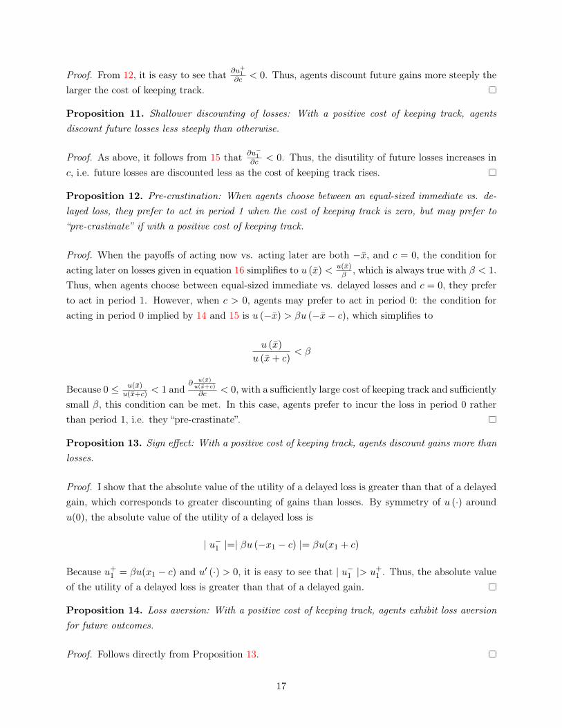
Proof. From 12, it is easy to see that ∂u+1

∂c < 0. Thus, agents discount future gains more steeply thelarger the cost of keeping track.

Proposition 11. Shallower discounting of losses: With a positive cost of keeping track, agentsdiscount future losses less steeply than otherwise.

Proof. As above, it follows from 15 that ∂u−1∂c < 0. Thus, the disutility of future losses increases in

c, i.e. future losses are discounted less as the cost of keeping track rises.

Proposition 12. Pre-crastination: When agents choose between an equal-sized immediate vs. de-layed loss, they prefer to act in period 1 when the cost of keeping track is zero, but may prefer to“pre-crastinate” if with a positive cost of keeping track.

Proof. When the payoffs of acting now vs. acting later are both −x̄, and c = 0, the condition foracting later on losses given in equation 16 simplifies to u (x̄) < u(x̄)

β , which is always true with β < 1.Thus, when agents choose between equal-sized immediate vs. delayed losses and c = 0, they preferto act in period 1. However, when c > 0, agents may prefer to act in period 0: the condition foracting in period 0 implied by 14 and 15 is u (−x̄) > βu (−x̄− c), which simplifies to

u (x̄)

u (x̄+ c)< β

Because 0 ≤ u(x̄)u(x̄+c) < 1 and

∂u(x̄)

u(x̄+c)

∂c < 0, with a sufficiently large cost of keeping track and sufficientlysmall β, this condition can be met. In this case, agents prefer to incur the loss in period 0 ratherthan period 1, i.e. they “pre-crastinate”.

Proposition 13. Sign effect: With a positive cost of keeping track, agents discount gains more thanlosses.

Proof. I show that the absolute value of the utility of a delayed loss is greater than that of a delayedgain, which corresponds to greater discounting of gains than losses. By symmetry of u (·) aroundu(0), the absolute value of the utility of a delayed loss is

| u−1 |=| βu (−x1 − c) |= βu(x1 + c)

Because u+1 = βu(x1 − c) and u′ (·) > 0, it is easy to see that | u−1 |> u+

1 . Thus, the absolute valueof the utility of a delayed loss is greater than that of a delayed gain.

Proposition 14. Loss aversion: With a positive cost of keeping track, agents exhibit loss aversionfor future outcomes.

Proof. Follows directly from Proposition 13.

17

Proposition 15. Magnitude effect: With a positive cost of keeping track, agents discount largeamounts less than small amounts.

Proof. The magnitude effect requires that the discounted utility of a large payoff Ax (A > 1) belarger, in percentage terms relative to the undiscounted utility of the same payoff, than that of asmaller payoff x:

βu(Ax− c)u(Ax)

>βu(x− c)u(x)

By concavity of u(·), and given that A > 1,

u(Ax+ c)− u(Ax) < u(x+ c)− u(x)

Because u (·) is monotonically increasing, u(Ax) > u(x), and therefore:

u(Ax+ c)− u(Ax)

u(Ax)<u(x+ c)− u(x)

u(x)

Adding one on both sides and decreasing the arguments by c:

u(Ax)

u(Ax− c)<

u(x)

u(x− c)

Inverting the fractions and multiplying both sides by β, we obtained the desired result.

Proposition 16. Decreasing impatience and preference reversals: With a positive cost of keepingtrack, agents exhibit decreasing impatience and time-inconsistent preference reversals.

Proof. When both outcomes are moved one period into the future, they are both subject to the riskand penalty of forgetting; their utilities are:

u1 = βu(x0 − c)

u2 = β2u(x1 − c)

The condition for acting later is

u (x1 − c) >u (x0 − c)

β

Note that, because u(·) is monotonically increasing and therefore u(x0−c) < u(x0), this condition iseasier to meet than condition 13 for choosing between acting immediately vs. next period, which isu (x1 − c) > u(x0)

β . Thus, when both outcomes are delayed into the future, impatience decreases.

18

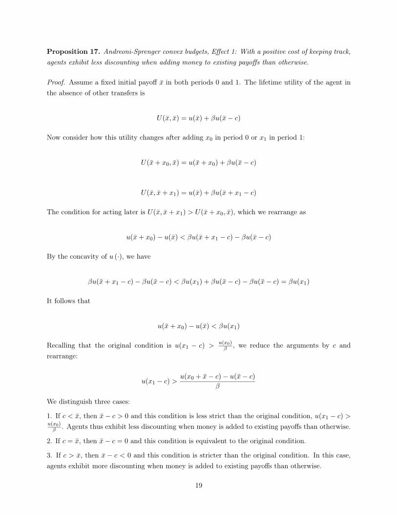
Proposition 17. Andreoni-Sprenger convex budgets, Effect 1: With a positive cost of keeping track,agents exhibit less discounting when adding money to existing payoffs than otherwise.

Proof. Assume a fixed initial payoff x̄ in both periods 0 and 1. The lifetime utility of the agent inthe absence of other transfers is

U(x̄, x̄) = u(x̄) + βu(x̄− c)

Now consider how this utility changes after adding x0 in period 0 or x1 in period 1:

U(x̄+ x0, x̄) = u(x̄+ x0) + βu(x̄− c)

U(x̄, x̄+ x1) = u(x̄) + βu(x̄+ x1 − c)

The condition for acting later is U(x̄, x̄+ x1) > U(x̄+ x0, x̄), which we rearrange as

u(x̄+ x0)− u(x̄) < βu(x̄+ x1 − c)− βu(x̄− c)

By the concavity of u (·), we have

βu(x̄+ x1 − c)− βu(x̄− c) < βu(x1) + βu(x̄− c)− βu(x̄− c) = βu(x1)

It follows that

u(x̄+ x0)− u(x̄) < βu(x1)

Recalling that the original condition is u(x1 − c) > u(x0)β , we reduce the arguments by c and

rearrange:

u(x1 − c) >u(x0 + x̄− c)− u(x̄− c)

β

We distinguish three cases:

1. If c < x̄, then x̄− c > 0 and this condition is less strict than the original condition, u(x1 − c) >u(x0)β . Agents thus exhibit less discounting when money is added to existing payoffs than otherwise.

2. If c = x̄, then x̄− c = 0 and this condition is equivalent to the original condition.

3. If c > x̄, then x̄ − c < 0 and this condition is stricter than the original condition. In this case,agents exhibit more discounting when money is added to existing payoffs than otherwise.

19

Note that if c > x̄, the cost of keeping track c exceeds the fixed initial payoff x̄. Under thesecircumstances, the agent would not initially have chosen to receive the fixed initial payoff andinstead preferred to not receive money at the timepoint in question; put differently, she would haveforgone the opportunity. Thus, when money is added to existing payoffs, it must be the case thatc ≤ x̄. This proves the proposition.

Finally we ask whether agents exhibit less hyperbolic discounting when money is added to existingpayoffs and the utility function is concave. This is the only result that holds with linear utility, butdoes not hold with concave utility. In fact, with concave utility, agents exhibit more hyperbolicitywhen money is added to existing payoffs than otherwise.

Proposition 18. Andreoni-Sprenger convex budgets, Effect 2: With a positive cost of keeping track,agents exhibit more hyperbolic discounting when adding money to existing payoffs.

Proof. Recall the case with no fixed intial payoff x̄. The condition for acting in period 1 over period0 is

(1) βu(x1 − c) > u(x0) (17)

When both periods are in the future, the condition for acting in period 2 over period 1 is

(2) βu(x1 − c) > u(x0 − c) (18)

Note that condition 17 is less strict than condition 18; this implies hyperbolic discounting, as thecondition for acting in the future is easier to meet when both periods are in the future than whenone is in the present.

Now assume a fixed initial payoff x̄ in both periods. The condition for acting in period 1 over period0 is

(3) u(x̄) + βu(x̄+ x1 − c) > u(x̄+ x0) + βu(x̄− c) (19)

When both periods are in the future, the condition for acting in period 2 over period 1 is

(4) u(x̄− c) + βu(x̄+ x1 − c) > u(x̄+ x0 − c) + βu(x̄− c) (20)

Rearranging 19 and 20, we obtain:

(5) u(x̄+ x0)− u(x̄) < βu(x̄+ x1 − c)− βu(x̄− c) (21)

20

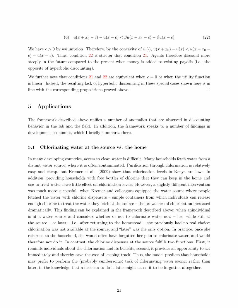
(6) u(x̄+ x0 − c)− u(x̄− c) < βu(x̄+ x1 − c)− βu(x̄− c) (22)

We have c > 0 by assumption. Therefore, by the concavity of u (·), u(x̄+ x0)− u(x̄) < u(x̄+ x0 −c) − u(x̄ − c). Thus, condition 22 is stricter that condition 21. Agents therefore discount moresteeply in the future compared to the present when money is added to existing payoffs (i.e., theopposite of hyperbolic discounting).

We further note that conditions 21 and 22 are equivalent when c = 0 or when the utility functionis linear. Indeed, the resulting lack of hyperbolic discounting in these special cases shown here is inline with the corresponding propositions proved above.

5 Applications

The framework described above unifies a number of anomalies that are observed in discountingbehavior in the lab and the field. In addition, the framework speaks to a number of findings indevelopment economics, which I briefly summarize here.

5.1 Chlorinating water at the source vs. the home

In many developing countries, access to clean water is difficult. Many households fetch water from adistant water source, where it is often contaminated. Purification through chlorination is relativelyeasy and cheap, but Kremer et al. (2009) show that chlorination levels in Kenya are low. Inaddition, providing households with free bottles of chlorine that they can keep in the home anduse to treat water have little effect on chlorination levels. However, a slightly different interventionwas much more successful: when Kremer and colleagues equipped the water source where peoplefetched the water with chlorine dispensers – simple containers from which individuals can releaseenough chlorine to treat the water they fetch at the source – the prevalence of chlorination increaseddramatically. This finding can be explained in the framework described above: when anindividualis at a water source and considers whether or not to chlorinate water now – i.e. while still atthe source – or later – i.e., after returning to the homestead – she previously had no real choice:chlorination was not available at the source, and “later” was the only option. In practice, once shereturned to the household, she would often have forgotten her plan to chlorinate water, and wouldtherefore not do it. In contrast, the chlorine dispenser at the source fulfills two functions. First, itreminds individuals about the chlorination and its benefits; second, it provides an opportunity to actimmediately and thereby save the cost of keeping track. Thus, the model predicts that householdsmay prefer to perform the (probably cumbersome) task of chlorinating water sooner rather thanlater, in the knowledge that a decision to do it later might cause it to be forgotten altogether.

21

5.2 Nudging farmers to use fertilizer

Developing economies are often characterized by surprisingly low levels of adoption of profitabletechnologies. A prime example is agricultural fertilizer, which is widely available and affordablein countries such as Kenya, and increases yields substantially. Nevertheless, few farmers reportusing fertilizer, even though many report wanting to use it. Duflo et al. (2009) show that a simpleintervention can substantially increase fertilizer use: by offering timed discounts on fertilizer tofarmers immediately after the harvest (when liquidity is high), rather than before the next plantingseason (when fertilizer would normally be bought, but liquidity is low), Duflo and colleagues providedfarmers with both a reminder of their desire to use fertilizer, as well as with an opportunity to actimmediately. As in the chlorine example, buying fertilizer is an expense, and therefore, assumingconstant prices, standard discounting models would predict that farmers should delay it as much aspossible. However, in Duflo et al.’s study, farmers pre-crastinate because they anticipate that theywill fail to buy fertilizer with a non-zero probability if they delay it. This cost of keeping track issomewhat different than those discussed above – in particular, it is unlikely to stem from forgettingbecause the need to purchase fertilizer probably becomes ever more salient as the planting seasonapproaches. Instead, it is likely that keeping track in this case consists of keeping track of theincome from the last harvest and avoiding to spend it on other goods, with the result that nothingis left to buy fertilizer before the planting season.

5.3 Getting children vaccinated

Many children in developing countries do not receive the standard battery of vaccinations, evenwhen these vaccinations are safe and available free of charge. Banerjee et al. (2010) organized andadvertised immunization camps in 130 villages in rural India, to which mothers could bring theirchildren to have them immunized. In a subset of villages, mothers additionally received a smallincentive when they brought their children to get vaccinated. Banerjee and colleagues find thatvaccination rates increase dramatically as a result of this program. Interpreted in the frameworkpresented in this paper, we might suspect that women remember at random times that they valuevaccinations and want to get their children vaccinated. However, these thoughts may often occurwhen no good opportunity exists to act on the thought – e.g., while performing other work, or atnight. The vaccination camps might combine a reminder of the desire to get children vaccinatedwith a concrete opportunity to follow through on this desire.

5.4 Reminders to save

The savings rates of the poor are generally low, despite the fact that they often have disposableincome that could in principle be saved. Karlan et al. (2010) show that savings rates among poorindividuals in the Philippines, Peru, and Bolivia can be substantially increased through simple textmessage (SMS) reminders to save. This finding confirms that the poor in fact do have disposable

22

income which they can save, and that they have a desire to do so. The fact that reminders alonecan make them more successful in reaching this goal suggests that they may on occasion simplyforget their savings goal and instead spend on other goods. The reminders transiently reduce thecost of keeping track to zero and thus allow households to follow through on their goal.

Note that the model predicts that reminders work because they decrease the cost of keeping track:if an individual is credibly offered a reminder, her cost of keeping track is reduced, so she is morelikely to wait and successfully perform the task. However, the model also predicts that timing iscrucial: if a reminder comes at a time when the agent can act on it, the probability that it issuccessful should be very high. In contrast, when the agent currently cannot act on it, the agent isin the previous situation of having to make a plan to act on the reminder later, making it less likelyto happen because of the cost of keeping track.

5.5 Status quo bias, default choice, and technology adoption

The phenomenon that people stick to defaults can be explained in the same framework. As pointedout above, tasks and opportunities arise at random points in time; this includes thoughts such as“I should really get a 401k”. The model predicts that people are much less likely to act on suchthoughts when they occur at times where acting on them immediately is not possible. In such cases,the agents make plans to act on the thought in the future, but these plans are subject to thec costof keeping track and therefore less likely to be implemented. Examples include the tendency tostick to defaults in organ donation and retirement plan decisions. Another prominent example isthe failure to adopt profitable technologies often found in developing countries; this phenomenon isa special case of default choice, and is also captured by the model.

6 Conclusion

This paper has argued that a number of features of empirically observed discount functions canbe explained with a lump-sum cost of keeping track of future transactions. First, such a cost willcause agents to discount the future more than they otherwise would; for instance, agents whose timepreference coincides with the interest rate will exhibit behavior that appear much more impatientwith a positive cost of keeping track. Second, if the cost is constant across time, agents will exhibitdecreasing impatience, i.e. they will discount the near future more than the distant future. Third,if the cost is lump-sum, agents will also exhibit a magnitude effect, i.e. they will discount smallerpayoffs more heavily than larger payoffs. Fourth, because the cost of keeping track is subtractedfrom gains, but is also subtracted from losses, the model produces a sign effect: a loss is discountedless than a gain of equal magnitude, both because the gain is less attractive due to the cost ofkeeping track than otherwise, and because the loss is more painful due to the cost of keepingtrack. Fifth, this result of the model also implies loss aversion for future outcomes, which is a

23

hallmark of prospect theory (Kahneman & Tversky, 1979). Sixth, the magnitude effect also impliesthat agents exhibit less discounting when money is added to existing payoffs in the present and thefuture, and that agents exhibit no decreasing impatience under these circumstances; this finding hasrecently been empirically confirmed by Andreoni & Sprenger (2012). Seventh, the model predictspre-crastination: when the cost of keeping track is large enough, agents will prefer to incur lossessooner rather than later. For instance, they may prefer to get a bill payment out of the way ifthey anticipate a risk of forgetting about the payment (and an associated penalty) in case theypostpone it. This phenomenon is familiar from everyday experience, but is currently not capturedby discounting models. Pre-crastination has also recently been empirically confirmed (Rosenbaumet al., 2014). Eighth, the model also predicts status quo bias and the choice of defaults: agentsmay appear to be unwilling to adopt profitable technologies or stick to disadvantageous defaultsdespite the presence of superior alternatives. The model suggests that these behaviors need notreflect preferences, but either an inability to act on such opportunities at the time when individualsthink about them (e.g. no chlorine dispenser at the source while fetching water), or, in the casewhere the cost of keeping track is small enough that agents make plans to act later, the risk offorgetting to act on the opportunity (forgetting to chlorinate water in the home after returningfrom the water source). Finally, the model predicts that simple reminders might cause individualsto act on opportunities that they previously appeared to dislike, and that reminders and/or creationof opportunities to act on tasks, such as bill payments, loan repayments, or taking medication, willincrease payment reliability and adherence. Indeed, a number of studies have shown positive effectsof reminders on loan repayment (e.g. Karlan et al., 2010).

A limitation of the current model is that it predicts that only sophisticates will exhibit the anomalousdiscounting behaviors summarized above, while naïve types will exhibit exponential discounting.To be sure, this leads to a welfare loss for the naïve type if they underestimate their probabilityof forgetting future tasks and opportunities and therefore are more likely to incur the associatedpenalties; but it generates the somewhat surprising prediction that sophisticated decision-makerswill appear more “anomalous” in their discounting behavior than naïve types.

Together, these results unify a number of disparate features of empirically observed discountingbehavior, as well as behavior of individuals in domains such as loan repayment, medication adher-ence, and technology adoption. The model makes quantitative predictions about the effectivenessof reminders, which should be experimentally tested.

24

References

1. Andreoni, James, and Charles Sprenger. 2012. “Estimating Time Preferences from ConvexBudgets.” American Economic Review 102 (7): 3333–56. doi:10.1257/aer.102.7.3333.

2. Banerjee, Abhijit Vinayak, Esther Duflo, Rachel Glennerster, and Dhruva Kothari. 2010. “Im-proving Immunisation Coverage in Rural India: Clustered Randomised Controlled Evaluationof Immunisation Campaigns with and without Incentives.” BMJ (Clinical Research Ed.) 340:c2220.

3. Duflo, Esther, Michael Kremer, and Jonathan Robinson. 2009. “Nudging Farmers to UseFertilizer: Theory and Experimental Evidence from Kenya.” National Bureau of EconomicResearch Working Paper.

4. Kahneman, D., and A. Tversky. 1979. “Prospect Theory: An Analysis of Decision underRisk.” Econometrica: Journal of the Econometric Society, 263–91.

5. Karlan, Dean, Margaret McConnell, Sendhil Mullainathan, and Jonathan Zinman. 2010.“Getting to the Top of Mind: How Reminders Increase Saving.” National Bureau of EconomicResearch Working Paper.

6. Kremer M, Miguel E, Mullainathan S, Null C, Zwane A. 2009a. Coupons, promoters, anddispensers: impact evaluations to increase water treatment. Work. Pap.

7. Laibson, David. 1997. “Golden Eggs and Hyperbolic Discounting.” The Quarterly Journal ofEconomics 112 (2): 443–78. doi:10.1162/003355397555253.

8. Mullainathan, Sendhil, and Eldar Shafir. Scarcity: Why Having Too Little Means So Much.

9. Rosenbaum, David A., Lanyun Gong, and Cory Adam Potts. 2014. “Pre-Crastination Has-tening Subgoal Completion at the Expense of Extra Physical Effort.” Psychological Science,May, 0956797614532657. doi:10.1177/0956797614532657.

10. Strotz, Robert H., “Myopia and Inconsistency in Dynamic Utility Maximization,” Review ofEconomic Studies, XXIII (1956), 165–80.

11. Wixted, John T. 2004. “On Common Ground: Jost’s (1897) Law of Forgetting and Ribot’s(1881) Law of Retrograde Amnesia.” Psychological Review 111 (4): 864–79. doi:10.1037/0033-295X.111.4.864.

25

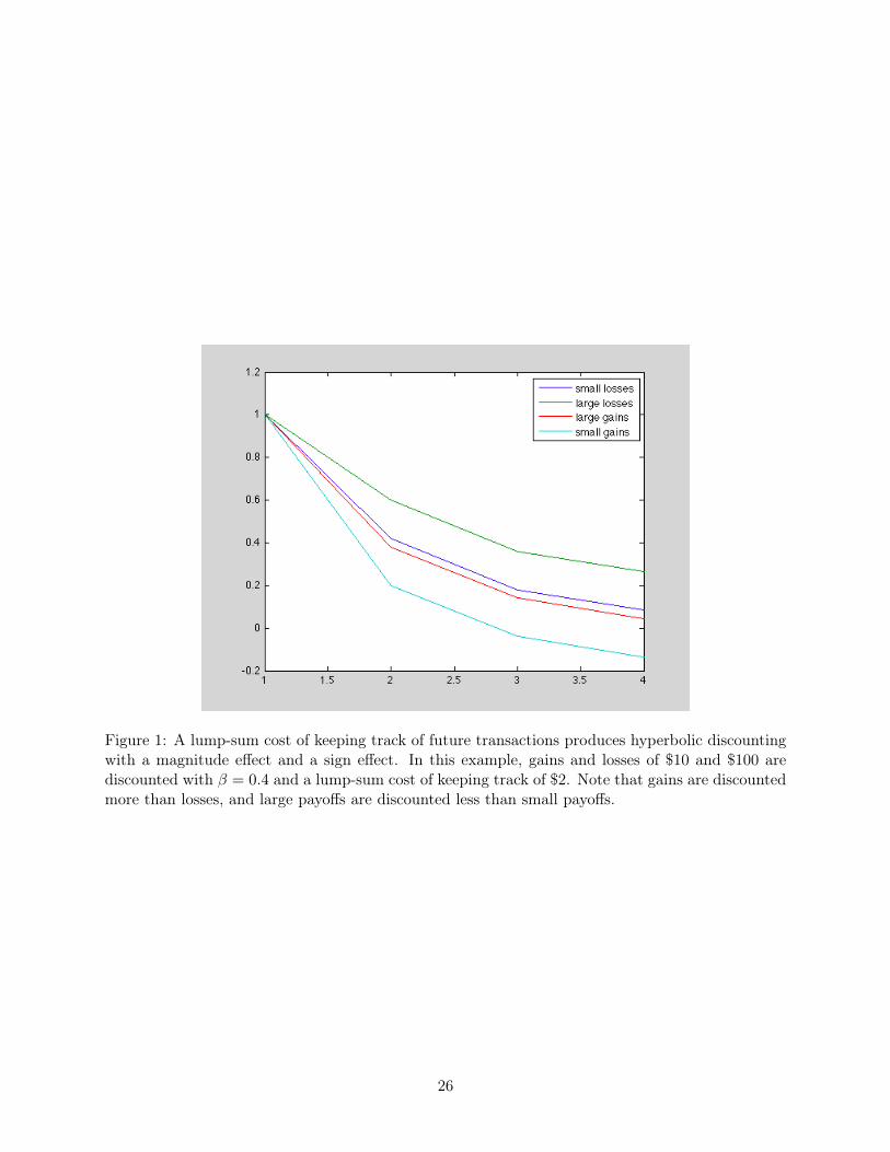
Figure 1: A lump-sum cost of keeping track of future transactions produces hyperbolic discountingwith a magnitude effect and a sign effect. In this example, gains and losses of $10 and $100 arediscounted with β = 0.4 and a lump-sum cost of keeping track of $2. Note that gains are discountedmore than losses, and large payoffs are discounted less than small payoffs.

26