The Delivery Man Problem With Time Windows

Discrete Optimization 7 (2010) 269–282

Contents lists available at ScienceDirect

Discrete Optimization

journal homepage: www.elsevier.com/locate/disopt

The Delivery Man Problem with time windows

Géraldine Heilporn a,b, Jean-François Cordeau a, Gilbert Laporte b,∗

a Canada Research Chair in Logistics and Transportation and CIRRELT, HEC Montréal, 3000 chemin de la Côte-Sainte-Catherine, Montréal, Canada H3T 2A7b Canada Research Chair in Distribution Management and CIRRELT, HEC Montréal, 3000 chemin de la Côte-Sainte-Catherine, Montréal, Canada H3T 2A7

a r t i c l e i n f o

Article history:Received 30 September 2009Received in revised form 12 March 2010Accepted 21 June 2010Available online 15 July 2010

Keywords:Delivery Man ProblemTraveling Salesman ProblemTime windowsPolyhedral analysisMixed integer linear programming

a b s t r a c t

In this paper, a variant of the Traveling Salesman Problem with Time Windows isconsidered, which consists in minimizing the sum of travel durations between a depotand several customer locations. Two mixed integer linear programming formulations arepresented for this problem: a classical arc flow model and a sequential assignment model.Several polyhedral results are provided for the second formulation, in the special casearising when there is a closed time window only at the depot, while open time windowsare considered at all other locations. Exact and heuristic algorithms are also proposed forthe problem. Computational results show thatmedium size instances can be solved exactlywith both models, while the heuristic provides good quality solutions for medium to largesize instances.

© 2010 Elsevier B.V. All rights reserved.

1. Introduction

The Delivery Man Problemwith TimeWindows (DMPTW) is a variant of the Traveling Salesman Problemwith TimeWindows(TSPTW) defined as follows. Let G = (N ∪ {0}, A) be a complete directed and asymmetric graph, where N = {1, . . . , n}is a set of delivery nodes and 0 is the depot. A travel time cij is associated with each arc (i, j) ∈ A. Time windows areimposed on the beginning of service at the nodes of G: earliest and latest times are described by parameters ei and li fornodes i ∈ N ∪ {0}. If node i is reached before ei, waiting occurs before service begins at this node. We also define the travelduration of node i as the difference between the beginning of service at node i and the beginning of service at the depot.The DMPTW consists in determining a Hamiltonian path on G, starting at the depot node 0, so as to minimize the sum oftravel durations over all nodes i ∈ N while respecting time windows. The cumulative objective function of the DMPTW iswell suited to real applications involving passengers or perishable goods as, for instance, school bus routing and scheduling,the transportation of disabled people, and even some postal deliveries. Further, note that the time needed to go back to thedepot is not included in the objective function. This means that we only care about the travel durations of the passengersor perishable goods. Similar problems, i.e., without a return to the depot, are referred to as ‘open vehicle routing problems’(see for instance [1,2] or [3]).The literature on the DMPTW is very limited. The only paper we are aware of is the one from Tsitsiklis [4], who presented

NP-completeness results or polynomial algorithms for several special cases of the TSPTW and DMPTW. The Delivery ManProblem (DMP) (also called Traveling Repairman Problem), i.e., a DMPTW without time windows, was introduced byLucena [5] who proposed an integer nonlinear model for the problem. The author derived lower bounds by Lagrangianrelaxation and solved instances with up to 30 nodes using an enumerative algorithm. Fischetti et al. [6], van Eijl [7] andMéndez-Díaz et al. [8] presented several mixed integer linear programming formulations and valid inequalities for the

∗ Corresponding author.E-mail address: [email protected] (G. Laporte).

1572-5286/$ – see front matter© 2010 Elsevier B.V. All rights reserved.doi:10.1016/j.disopt.2010.06.002

http://www.elsevier.com/locate/disopt

http://www.elsevier.com/locate/disopt

mailto:[email protected]

http://dx.doi.org/10.1016/j.disopt.2010.06.002

270 G. Heilporn et al. / Discrete Optimization 7 (2010) 269–282

DMP, and solved instances having between 15 and 60 nodes. The Méndez-Díaz et al. formulation with precedence variablesoutperforms all others in terms of relaxation quality and provides good results for instances involving up to 40 nodes. Notethat the DMP is also known as theMinimum Latency Problem (MLP) in the scheduling literature, inwhich themostmentionedapplication concerns disk-head scheduling. Several authors have proposed approximation algorithms for the MLP (see, forinstance, [9,10] or [11]). Wu et al. [12] also presented an exact algorithm combining dynamic programming and branch-and-bound, and solved instances with up to 26 nodes. However, neither the DMP nor the MLP includes time windows andthe corresponding formulations cannot be adapted to the DMPTW.The TSPTW has been more extensively studied. Baker [13] proposed a non-differentiable and non-convex model and

solved instanceswith up to 50 nodes by branch-and-bound, using a longest path algorithm to obtain lower bounds. Langevinet al. [14] presented a mixed integer linear formulation based on a two-commodity network flow and solved instances withup to 60 nodes. However, their formulation is not well suited to include a cumulative objective function. Ascheuer et al. [15]developed valid inequalities for the TSPTW and proved several polyhedral results. In a companion paper, Ascheuer et al. [16]compared three mixed integer linear formulations for the problem. They developed a branch-and-cut algorithm for theirbestmodelwhich is capable of solving instanceswith up to 70 nodes. For the same formulation,Mak and Ernst [17] proposednew cycle breaking and infeasible path inequalities. Preliminary results have shown that these tighten the optimality gapbut no further numerical results were presented. However, because the latter formulation makes use of infeasible pathinequalities to model time windows, it cannot handle a cumulative objective function either.Since both DMP and TSPTW are NP-hard, several authors have focused on heuristics. For the DMP, Lucena [5] and Bianco

et al. [18] have proposed 2-exchange amd 3-exchange heuristics, respectively, the initial tour being constructed by aninsertion procedure. They solved instances with up to 35 nodes. A 3-exchange heuristic, coupled with a greedy initializationprocedure, was also considered by Fischetti et al. [6]. The authors solved instances with up to 60 nodes. In what concerns theTSPTW, Gendreau et al. [19] proposed an adaptation of a near-optimal TSP heuristic, and obtained good quality solutions forinstanceswith up to 100nodes.Wolfler Calvo [20] developed a heuristic inwhich a related assignment problem is first solvedto minimize infeasibility with respect to time windows. The corresponding solution is then reduced to a single tour andimproved by a local search procedure. He solved instances with up to 200 nodes, and obtained better results than Gendreauet al. Note that other techniques have also been used to solve both DMP and TSPTW. Bianco et al. [18] solved instances ofthe DMP with up to 60 nodes with dynamic programming. Dumas et al. [21] and Bianco et al. [22] solved instances of theTSPTW with between 120 and 200 nodes again using dynamic programming, while Pesant et al. [23] and Focacci et al. [24]combined constraint-programming and exact optimization methods, and solved instances with up to 40 nodes.The aim of this paper is to analyse and solve the DMPTW.We present mixed integer linear formulations for the problem,

together with exact and heuristic algorithms. We also perform a polyhedral analysis of a special case. If all time windowsare closed (i.e., earliest and latest times are given for all locations), finding a feasible solution is NP-hard [25]. Then thedimension of the convex hull of feasible solutions cannot be determined, and no further polyhedral results can be derived.However, this is not the case if a closed time window is imposed only at the depot and all other nodes have an open timewindow, as in [15]. We perform a separate analysis of this particular case.The remainder of this paper is organized as follows. Two formulations of the DMPTW are presented in Sections 2 and

3. The first one is a classical model involving arc flow variables, while the second is a sequential assignment model thatexplicitly considers the position of nodes in theHamiltonian path. Valid inequalities and polyhedral results are developed forthe new sequential assignment formulation. Exact and heuristic algorithms are proposed in Section 4. Finally, computationalresults are presented in Section 5, followed by conclusions in Section 6.

2. Classical arc flow formulation

According to the Öncan et al. survey [26] in which several Asymmetric Traveling Salesman Problem (ATSP) formulationsare compared, the best models are those that include precedence variables in addition to standard arc flow variables. Weadapt such a formulation presented by Gouveia and Pires [27]. Let xij : i, j ∈ N ∪ {0}(i 6= j) be arc flow variables, whilevij : i, j ∈ N(i 6= j) and f kij : i, k ∈ N, j ∈ N ∪ {0}(i 6= j), represent precedence variables:

vij =

{1 if node i precedes node j in the Hamiltonian path,0 otherwise (1)

f kij ={1 if arc (i, j) appears after node k in the Hamiltonian path,0 otherwise. (2)

Finally, in order to deal with the cumulative objective function, variables ti : i ∈ N ∪ {0} are introduced to represent thetimes at which service begins at the nodes.With this notation, the DMPTW can be modelled as follows:

(AF-DMP) minimizen∑i=1

(ti − t0) (3)

G. Heilporn et al. / Discrete Optimization 7 (2010) 269–282 271

subject to:ti + cij ≤ tj +Mij(1− xij) i ∈ N ∪ {0}, j ∈ N(i 6= j) (4)

t0 ≤ tj j ∈ N (5)

ej ≤ tj ≤ lj j ∈ N (6)

e0 ≤ t0 ≤ l0 (7)∑i∈N∪{0}

xij = 1 j ∈ N ∪ {0} (8)

∑j∈N∪{0}

xij = 1 i ∈ N ∪ {0} (9)

∑i∈N∪{0}

f kji −∑i∈N

f kij = 0 j, k ∈ N(j 6= k) (10)

∑i∈N∪{0}

f jji = 1 j ∈ N (11)

f kij ≤ xij i, j, k ∈ N(i 6= j) (12)∑j∈N∪{0}

f kij = vki i, k ∈ N(i 6= k) (13)

∑p,q∈S

xpq + vki − vkj ≤ |S| − 1 i, j, k ∈ N(i 6= j 6= k) S ⊂ N, |S| ≥ 2 : i, j ∈ S, k 6∈ S (14)

f kij ≥ 0 i, j, k ∈ N(i 6= j) (15)

xij ∈ {0, 1} i, j ∈ N ∪ {0}(i 6= j), (16)whereMij : i ∈ N ∪ {0}, j ∈ N are sufficiently large constants.Constraints (4) and (5) are the schedule compatibility inequalities: they state that if an arc (i, j) is used, then the service

time at node j is at least equal to the service time at node i plus the travel time from i to j. They also ensure that node 0 isvisited before any node of N . Note that constraints (4) also eliminate subtours. Constraints (6) and (7) are the time windowsinequalities for nodes in N ∪{0}. Constraints (8) and (9) are arc flow inequalities. Constraints (10) and (11) are precedence flowinequalitieswhich ensure the flow conservation for variables f . Constraints (12) and (13) link the variables x, f and v. Finally,constraints (14) are the generalized subpath elimination inequalities, which prevent subpaths in G and link those with theprecedence variables v. Indeed, if node k precedes node i but not node j, there cannot be a path between nodes i and j and∑p,q∈S xpq ≤ |S|−2. Otherwise if node k precedes both i and j, or if nodes i and j precedes node k, then

∑p,q∈S xpq ≤ |S|−1.

Unfortunately, the schedule compatibility inequalities (4) involve ‘‘big-M’’ constants. As a consequence, a polyhedralstudy of model (AF-DMP) cannot be performed. Indeed, these constraints, which constitute an important part of thepolyhedral structure of the problem, would not define facets of the convex hull of feasible solutions of the model. Further,although the formulation (AF-DMP) is intuitive, it has been shown (see, e.g., [8] or [16]) that adding time variables to anATSP formulation is computationally expensive. For these reasons, an alternative more tractable model is presented in thenext section.

3. An alternative sequential assignment formulation

We now propose a new formulation for the DMPTW, which explicitly describes the node positions in the Hamiltonianpath. Such formulations have been considered in [28–30] for the Time-Dependent TSP, and also in [31] or [32] for SingleMachine Scheduling Problems.Let σ0 be the service time at node 0, and let σt : t = 1, . . . , n be the service time at the tth node of N . We introduce

position variables yjt : j ∈ N, t = 1, . . . , n and transition variableswtij : i, j ∈ N(i 6= j), t = 2, . . . , n, where

yjt ={1 if node j is the tth node of N in the Hamiltonian path,0 otherwise, (17)

wtij =

{1 if nodes i and j are respectively the (t − 1)st and tth nodes of Nin the Hamiltonian path,

0 otherwise.(18)

With these variables, the DMPTW can be modelled as the following mixed integer linear programming model:

(S-DMP) minimizen∑t=1

(σt − σ0) (19)


subject to:

σ1 − σ0 ≥∑i,j∈N:i6=j

c0jw2ji (20)

σt − σt−1 ≥∑i,j∈N:i6=j

cijwtij t = 2, . . . , n (21)

e0 ≤ σ0 ≤ l0 (22)

σ1 ≥∑i,j∈N:i6=j

ejw2ji (23)

σ1 ≤∑i,j∈N:i6=j

ljw2ji (24)

σt ≥∑i,j∈N:i6=j

ejwtij t = 2, . . . , n (25)

σt ≤∑i,j∈N:i6=j

ljwtij t = 2, . . . , n (26)

∑j∈N

yjt = 1 t = 1, . . . , n (27)

n∑t=2

yjt = 1 j ∈ N (28)∑i∈N

wtij = yjt j ∈ N, t = 2, . . . , n (29)∑i∈N

wtji = yj,t−1 j ∈ N, t = 2, . . . , n (30)

yjt ∈ {0, 1} j ∈ N, t = 1, . . . , n (31)

wtij ≥ 0 i, j ∈ N(i 6= j), t = 2, . . . , n. (32)

Constraints (20) and (21) are the schedule compatibility inequalities. Constraints (22)–(26) are the time windowsinequalities. Constraints (27) and (28) are the flow inequalities: (27) impose that a node is visited in each position t =1, . . . , n, whereas (28) ensure that each node is visited once. Finally, constraints (29) and (30) link the transition and positionvariableswtij and yjt .Note that, thanks to the introduction of the binary position variables yjt , the transition variables wtij can be declared as

continuous as one can check that wtij = yi,t−1yjt . Alternatively, the problem could be expressed in terms of the variables σtand wtij only, which would increase the number of binary variables from O(n

2) to O(n3). However, preliminary tests haveshown that the previous (S-DMP) provides the best computational performance.

3.1. Polyhedral study

As mentioned in Section 1, even finding a feasible solution to the DMPTW is NP-hard (see [25]). In order to assess thestrength of the formulation (S-DMP) from a theoretical viewpoint, we thus perform a polyhedral study of the particularsituation arising when a closed time window is imposed only at the depot, and all other nodes have an open time window.More specifically, we show that in this particular case, most constraints of model (S-DMP) define facets of the convex hullof feasible solutions.Let P E

= {(σ ,w) : (20)–(23) and (25), (27)–(32)} denote the convex hull of feasible solutions for model (S-DMP) inthe particular case described above. To avoid considering irrelevant cases, it is assumed that e0 < l0 and that the timewindows have been tightened so that ej = max{ej, e0 + c0j} for all j ∈ N . Let us also define a ‘‘path-w matrix’’ as anincidence matrix in which each row corresponds to a Hamiltonian path and each column corresponds to a variable wtij :i, j ∈ N(i 6= j), t = 2, . . . , n. The next lemma provides the rank of the path-w matrix.

Lemma 1. The rank of the path-w matrix is n3 − 3n2 + 2n.

This result is stated in [33]. We provide a proof in the Appendix. From this lemma, we can deduce the dimension of P E .One should note that the next proofswillmake use of dominated feasible solutions ofP E . Indeed, when all timewindows

are open, except the one at the depot, the service time at the depot should be set as late as possible and all other service times


as early as possible. For this particular situation, the optimal service times are thus uniquely determined by the choice of aHamiltonian path. However, we recall that our aim is to theoretically assess formulation (S-DMP). For this reason, we havedecided to consider the convex hull of all feasible solutions rather that the polyhedron corresponding to the non-dominatedfeasible solutions.

Proposition 1. The dimension of P E is n3 − 3n2 + 3n.

Proof. Model (S-DMP) contains n+1+n2+n(n−1)2 variables, whereas the number of equality constraints is 2n(n−1)+2n.However, n− 1 of these constraints can be obtained by linear combinations of others. For instance, one has

∑j∈N yjn = 1 =∑

i,j∈N:i6=jwnij =

∑i∈N yi,n−1 = · · · =

∑i∈N yi1. As a consequence, dim(P

E ) ≤ (n+ 1+ n2+ n(n− 1)2)− (2n(n− 1)+ 2n−(n− 1)) ≤ n3 − 3n2 + 3n.One can also prove that there exist n3 − 3n2 + 3n + 1 affinely independent points in P E . In the following, the points

of P E will be described by their corresponding Hamiltonian path, for instance the path (0, 1, 2, . . . , n), together with anassignment of variables σt (t = 0, . . . , n).First, the Hamiltonian path (0, 1, 2, . . . , n)with the assignments

σ0 = e0; σt = max{et , σt−1 + c(t−1)t}, t = 1, . . . , n (33)σ0 = e0; σt = max{et , σt−1 + c(t−1)t}, t = 1, . . . , n− 1;

σn = max{en, σn−1 + c(n−1)n} + ε (34)σ0 = e0; σt = max{et , σt−1 + c(t−1)t}, t = 1, . . . , n− 2;

σt = max{et , σt−1 + c(t−1)t} + ε, t = n− 1, n (35). . .

σ0 = e0; σt = max{et , σt−1 + c(t−1)t} + ε, t = 1, . . . , n (36)

σ0 = e0 + ε; σt = max{et , σt−1 + c(t−1)t} + ε, t = 1, . . . , n (37)

yield n+ 2 affinely independent points of P E .We also knowby Lemma 1 that the rank of the path-wmatrix is n3−3n2+2n. Further, because the equalitywtij = yi,t−1yjt

holds for all i, j ∈ N(i 6= j) and t = 2, . . . , n, there exists a bijection between the assignment of variables wtij andyjt . If (0 = π(0), π(1), π(2), . . . , π(n)) is a Hamiltonian path in G, the corresponding variables σt : t = 0, . . . , ncan be set to σ0 = e0 and σt = max{eπ(t), σt−1 + cπ(t−1)π(t)} for all t = 1, . . . , n. Hence each row of the path-wmatrix represents a feasible solution of (S-DMP), among which n3 − 3n2 + 2n are affinely independent. Because thepath (0, 1, 2, . . . , n) used in the first part of the proof is also a row of the path-w matrix, this means that P E contains(n+ 2)+ (n3 − 3n2 + 2n)− 1 = n3 − 3n2 + 3n+ 1 affinely independent points. The result follows. �

Wenow prove that most constraints, or strengthened constraints, of model (S-DMP) define facets ofP E . We first presenta strengthened version of inequality (20), which defines a facet of P E under a realistic condition on the time windows.

Proposition 2. The inequality

σ1 − σ0 ≥∑i,j∈N:i6=j,l0+c0j≥ej

c0jw2ji +∑i,j∈N:i6=j,l0+c0j<ej

(ej − l0)w2ji (38)

is valid for (S-DMP). Further, it defines a facet of P E if and only if there exists k̃ ∈ N such that l0 + c0k̃ > ek̃.

Proof. To prove that the inequality is valid, assume that w2ji = 1 for some i, j ∈ N . If l0 + c0j ≥ ej, inequality (38) becomesσ1− σ0 ≥ c0j, which is valid by (20). Otherwise, i.e., if l0+ c0j < ej, inequality (38) yields σ1− σ0 ≥ ej− l0, which is valid by(22) and (23). Now consider a path (0 = π(0), k̃ = π(1), π(2), . . . , π(n)). Since l0 + c0k̃ > ek̃, the following assignmentsare feasible for the variables σ :

σ0 = l0; σ1 = l0 + c0k̃; σt = max{eπ(t), σt−1 + cπ(t−1)π(t)}, t = 2, . . . , n (39)σ0 = l0; σ1 = l0 + c0k̃; σt = max{eπ(t), σt−1 + cπ(t−1)π(t)}, t = 2, . . . , n− 1;

σn = max{eπ(n), σπ(n)−1 + c(π(n)−1)π(n)} + ε (40)σ0 = l0; σ1 = l0 + c0k̃; σt = max{eπ(t), σt−1 + cπ(t−1)π(t)}, t = 2, . . . , n− 2;

σt = max{eπ(t), σt−1 + cπ(t−1)π(t)} + ε, t = n− 1, n (41). . .

σ0 = l0; σ1 = l0 + c0k̃; σt = max{eπ(t), σt−1 + cπ(t−1)π(t)} + ε, t = 2, . . . , n (42)σ0 = l0 − ε; σ1 = l0 + c0k̃ − ε;

σt = max{eπ(t), σt−1 + cπ(t−1)π(t)}, t = 2, . . . , n. (43)


This yields n+ 1 affinely independent points ofP E . Furthermore, the rank of the path-w incidence matrix is n3 − 3n2 + 2nby Lemma 1. For any path (0 = π(0), π(1), π(2), . . . , π(n)) such that l0 + c0π(1) ≥ eπ(1) (resp. l0 + c0π(1) < eπ(1)), thecorresponding variables σ can be set to σ0 = l0, σ1 = l0 + c0π(1) (resp. σ0 = l0, σ1 = eπ(1)) and σt = max{eπ(t), σt−1 +cπ(t−1)π(t)} for all t = 2, . . . , n.Finally, assume that there does not exist any k ∈ N such that l0+c0k > ek. Then all points ofP E satisfying (38) at equality

also lie on the hyperplane σ0 = l0 by (22). The result follows. �

Corollary 1. Under the assumption that l0 + c0j ≥ ej for all j ∈ N and provided there exists k̃ ∈ N such that l0 + c0k̃ > ek̃,constraint (20) of (S-DMP) defines a facet of P E .

One can also prove that the schedule compatibility inequalities (21) and the time window inequalities (22) define facetsof P E .

Proposition 3. Constraints (21) of (S-DMP) define facets of P E .

Proof. Given t̃ ∈ {2, . . . , n}, we prove that σt̃ − σt̃−1 ≥∑i,j∈N:i6=j cijw

t̃ij is facet defining for P

E . First, the Hamiltonian path(0, 1, 2, . . . , n)with the following assignments for variables σ :

σ0 = e0; σt = max{et , σt−1 + c(t−1)t}, t = 1, . . . , t̃ − 2, t̃ + 1, . . . , n;

σt̃−1 = max{et̃−1, σt̃−2 + c(t̃−2)(t̃−1), et̃ − c(t̃−1)t̃}; σt̃ = σt̃−1 + c(t̃−1)t̃ (44)

σ0 = e0; σt = max{et , σt−1 + c(t−1)t}, t = 1, . . . , t̃ − 2, t̃ + 1, . . . , n− 1;σt̃−1 = max{et̃−1, σt̃−2 + c(t̃−2)(t̃−1), et̃ − c(t̃−1)t̃}; σt̃ = σt̃−1 + c(t̃−1)t̃;

σn = max{en, σn−1 + c(n−1)n} + ε (45). . .

σ0 = e0; σt = max{et , σt−1 + c(t−1)t}, t = 1, . . . , t̃ − 2;σt̃−1 = max{et̃−1, σt̃−2 + c(t̃−2)(t̃−1), et̃ − c(t̃−1)t̃}; σt̃ = σt̃−1 + c(t̃−1)t̃;

σt = max{et , σt−1 + c(t−1)t} + ε, t = t̃ + 1, . . . , n (46)

σ0 = e0; σt = max{et , σt−1 + c(t−1)t}, t = 1, . . . , t̃ − 2;σt̃−1 = max{et̃−1, σt̃−2 + c(t̃−2)(t̃−1), et̃ − c(t̃−1)t̃} + ε; σt̃ = σt̃−1 + c(t̃−1)t̃;

σt = max{et , σt−1 + c(t−1)t} + ε, t = t̃ + 1, . . . , n (47). . .

σ0 = e0 + ε; σt = max{et , σt−1 + c(t−1)t} + ε, t = 1, . . . , t̃ − 2, t̃ + 1, . . . , n;

σt̃−1 = max{et̃−1, σt̃−2 + c(t̃−2)(t̃−1), et̃ − c(t̃−1)t̃} + ε; σt̃ = σt̃−1 + c(t̃−1)t̃ (48)

yield n+ 1 affinely independent points of P E .Next, the rank of the path-w incidence matrix is n3 − 3n2 + 2n by Lemma 1. For any path (0 = π(0), π(1),

π(2), . . . , π(n)), the variablesσ can be set toσ0 = e0,σt = max{eπ(t), σt−1+cπ(t−1)π(t)} for all t = 1, . . . , t̃−2, t̃+1, . . . , n,σt̃−1 = max{eπ(t̃−1), σt̃−2 + cπ(t̃−2)π(t̃−1), eπ(t̃) − cπ(t̃−1)π(t̃)} and σt̃ = σt̃−1 + cπ(t̃−1)π(t̃). �

Proposition 4. Constraints (22) of (S-DMP) define facets of P E .

Proof. We show that σ0 ≥ e0 is facet defining for P E . The proof that σ0 ≤ l0 defines a facet of P E is obtained by replacinge0 with l0.First consider the Hamiltonian path (0, 1, 2, . . . , n) together with the corresponding variables σ :

σ0 = e0; σt = max{et , σt−1 + c(t−1)t}, t = 1, . . . , n (49)σ0 = e0; σt = max{et , σt−1 + c(t−1)t}, t = 1, . . . , n− 1;

σn = max{en, σn−1 + c(n−1)n} + ε (50)σ0 = e0; σt = max{et , σt−1 + c(t−1)t}, t = 1, . . . , n− 2;

σt = max{et , σt−1 + c(t−1)t} + ε, t = n− 1, n (51). . .

σ0 = e0; σt = max{et , σt−1 + c(t−1)t} + ε, t = 1, . . . , n, (52)

which yield n+ 1 affinely independent points of P E .Next, the rank of the path-w incidence matrix is still n3 − 3n2 + 2n, and the variables σ can be set to σ0 = e0 and

σt = max{eπ(t), σt−1 + cπ(t−1)π(t)} for all t = 1, . . . , n. The result follows. �


The time window inequality (23) also defines a facet of P E under some realistic condition on the parameters ei (i ∈N ∪ {0}).

Proposition 5. Constraints (23) of (S-DMP) is facet defining for P E if and only if there exists k̃ ∈ N such that e0 + c0k̃ < ek̃.

Proof. Consider a path (0 = π(0), k̃ = π(1), π(2), . . . , π(n))with the following assignments for variables σ :

σ0 = e0; σ1 = ek̃; σt = max{eπ(t), σt−1 + cπ(t−1)π(t)}, t = 1, . . . , n (53)σ0 = e0; σ1 = ek̃; σt = max{eπ(t), σt−1 + cπ(t−1)π(t)}, t = 1, . . . , n− 1;

σn = max{eπ(n), σn−1 + cπ(n−1)π(n)} + ε (54)σ0 = e0; σ1 = ek̃; σt = max{eπ(t), σt−1 + cπ(t−1)π(t)}, t = 1, . . . , n− 2;

σt = max{eπ(t), σt−1 + cπ(t−1)π(t)} + ε, t = n− 1, n (55). . .

σ0 = e0; σ1 = ek̃; σt = max{eπ(t), σt−1 + cπ(t−1)π(t)} + ε, t = 2, . . . , n (56)

σ0 = e0 + ε; σ1 = ek̃; σt = max{eπ(t), σt−1 + cπ(t−1)π(t)} + ε, t = 2, . . . , n. (57)

One obtains n + 1 affinely independent points of P E . Next, the rank of the path-w incidence matrix is n3 − 3n2 + 2n byLemma 1. For any path (0 = π(0), π(1), π(2), . . . , π(n)), the corresponding variables σ can be set to σ0 = e0, σ1 = eπ(1)and σt = max{eπ(t), σt−1 + cπ(t−1)π(t)} for all t = 2, . . . , n (indeed, recall that the time windows have been tightened sothat ej = max{ej, e0 + c0j} for all j ∈ N).To prove the result, assume by contradiction that e0 + c0k ≥ ek for all k ∈ N . Then all points of P E that satisfy (23) at

equality also lie on the hyperplane σ0 = e0 by (20). �

Finally, the time window inequality involving the second node of N in the Hamiltonian path can be strengthened. Theresulting constraint also defines a facet of P E .

Proposition 6. The inequality

σ2 ≥∑i,j∈N:i6=j

max{ei, ej + cji}w2ji (58)

defines a facet of P E if and only if there exist k̃1, k̃2 ∈ N such that ek̃1 + ck̃1 k̃2 < ek̃2 .

Proof. First assume that ej+cji ≥ ei for all i, j ∈ N . Then any point ofP E satisfying (58) at equality also lies on the hyperplaneσ1 =

∑i,j∈N:i6=j ejw

2ji by (21). Hence the condition stated in Proposition 6 is necessary, so that (58) is facet defining for P

E .In order to prove that the assumption is also sufficient, consider a Hamiltonian path (0 = π(0), k̃1 = π(1), k̃2 =

π(2), π(3), . . . , π(n)). The following settings for variables σ yield n+ 1 affinely independent points of P E :

σ0 = e0; σ1 = ek̃1; σ2 = ek̃2;

σt = max{eπ(t), σt−1 + cπ(t−1)π(t)}, t = 1, . . . , n (59)σ0 = e0; σ1 = ek̃1; σ2 = ek̃2;

σt = max{eπ(t), σt−1 + cπ(t−1)π(t)}, t = 1, . . . , n− 1;

σn = max{eπ(n), σn−1 + cπ(n−1)π(n)} + ε (60). . .

σ0 = e0; σ1 = ek̃1; σ2 = ek̃2;

σt = max{eπ(t), σt−1 + cπ(t−1)π(t)} + ε, t = 3, . . . , n (61)σ0 = e0; σ1 = ek̃1 + ε; σ2 = ek̃2;

σt = max{eπ(t), σt−1 + cπ(t−1)π(t)} + ε, t = 3, . . . , n (62)σ0 = e0 + ε; σ1 = ek̃1 + ε; σ2 = ek̃2;

σt = max{eπ(t), σt−1 + cπ(t−1)π(t)} + ε, t = 3, . . . , n. (63)

Note that the condition stated in Proposition 6 ensures the feasibility of the two last assignments for variables σ . Further-more, for any path (0 = π(0), π(1), π(2), . . . , π(n)), the corresponding variables σ can be set to σ0 = e0, σ1 = eπ(1),σ2 = max{eπ(2), eπ(1) + cπ(1)π(2)} and σt = max{eπ(t), σt−1 + cπ(t−1)π(t)} for all t = 3, . . . , n. As the rank of the path-wincidence matrix is n3 − 3n2 + 2n as before, the result follows. �

Hence only the time window inequalities involving the third to the nth node of N in the Hamiltonian path do notdefine facets of P E . This means that model (S-DMP) is strong, at least theoretically. In Section 5, the latest model will becomputationally compared with the classical model (AF-DMP).


4. Algorithms

In this section, we describe both an exact and a heuristic solution method for the DMPTW.

4.1. Exact algorithm

Models (AF-DMP) and (S-DMP) can be implemented and solved exactly using a general purpose branch-and-cutalgorithm. The subtour elimination constraints (14) in (AF-DMP) are separated in a classical way. Given a current solution,we create a supporting graph G∗ = (N ∪ {0}, A∗), where (i, j) ∈ A∗ has a capacity equal to the value x∗ij taken by xij. First, wedetermine the number of connected components in the graph induced by the arcs with strictly positive capacity. If there ismore than one connected component, the corresponding subtour elimination constraints are appended to the model. Next,for all i, j, k ∈ N , we aggregate the nodes i, j into a node ij, and we look for the minimum capacity cut between nodes ij andk. If the corresponding subtour elimination constraint (14) is violated by the current solution, it is appended to the model.For the DMPTWwith closed time windows at all nodes, the constantsMij of model (AF-DMP) are set toMij = li + cij − ej

for all i ∈ N ∪ {0} and j ∈ N . If a closed time window is imposed only at the depot and all nodes of N have an open timewindow, then we set the constantsMij as follows:

Mij = maxj∈N∪{0}

{ej} +∑k∈N:k6=j

maxj∈N{ckj} − cij i, j ∈ N (64)

M0j = maxj∈N∪{0}

{ej} +∑

k∈N∪{0}:k6=j

maxj∈N{ckj} − c0j j ∈ N. (65)

Furthermore, using logical implications between the time windows [ei, li] : i ∈ N and the travel times cij : i ∈ N ∪ {0},j ∈ N , the time windows are tightened as follows:

ej = max{ej, mini∈N∪{0}:i6=j

{ei + cij}}j ∈ N (66)

lj = min{lj,max

{ej, maxi∈N∪{0}:i6=j

{li + cij}}}

j ∈ N (67)

l0 = min{l0, maxi∈N:i6=j{li − c0i}

}. (68)

We also apply a preprocessing step on the nodes of N , setting xij = 0 in model (AF-DMP) (resp. wtij = 0 for all t = 2, . . . , nin (S-DMP)) for all i, j ∈ N such that ei + cij > lj.Finally, a strengthened version of model (S-DMP) is considered. In the latter, the facet defining inequalities (38) and (58)

are appended to (S-DMP), together with the following valid inequalities:

σ2 ≤∑i,j∈N:i6=j

min{li,max{ei, lj + cji}}w2ji (69)

σt ≥∑i,j∈N:i6=j

max{ej, ei + cij}wtij t = 3, . . . , n (70)

σt ≤∑i,j∈N:i6=j

min{lj,max{ej, li + cij}}wtij t = 3, . . . , n. (71)

The validity of these inequalities can be checked using logical implications between the schedule compatibility and the timewindow constraints. Furthermore, note that (69) and (71) are redundant when a closed time window is imposed only at thedepot.

4.2. Heuristic

Wenowdescribe a heuristic for theDMPTW.An insertion procedure is first applied to construct an initial feasible solutionof the problem. An exchange procedure is then used to perturb the current solution and to improve the objective functionvalue.The insertion procedure works as follows. As in [20], we solve a related Assignment Problem (AP) while minimizing

infeasibility of time windows. Because tj ≤ lj for all j ∈ N and considering the cumulative objective function of the DMPTW,the service times at nodes of N should be as small as possible. For all i ∈ N ∪ {0}, j ∈ N such that xij = 1, one also knowsthat

tj ≥ max{ti + cij, ej} ≥ max{ei + cij, ej} = ei + cij + w̄ij, (72)


where w̄ij = max{ej − ei − cij, 0}. Hence the following AP is solved:

(AP) minimize∑

i∈N∪{0},j∈N:i6=j

(cij + w̄ij)xij (73)

subject to:∑i∈N∪{0}

xij = 1 j ∈ N ∪ {0} (74)

∑j∈N∪{0}

xij = 1 i ∈ N ∪ {0}, (75)

xij ∈ {0, 1} i, j ∈ N ∪ {0}. (76)

The AP solution yields a main path (0, . . . , k) containing the depot 0, as well as several subpaths not containing it. Thefeasibility of the main path is then checked by computing the earliest times at nodes:

t0 = e0 (77)tj = max{ej, tj−1 + c(j−1)j} j ∈ {1, . . . , k}. (78)

If a node j ∈ N is infeasible with respect to its time window [ej, lj], i.e., if tj > lj, it is removed from the main path.Next, the subpaths are selected one at a time for insertion in the main path. At each iteration, the selected subpath S is

the one corresponding to the smallest time window width li − ei : i ∈ N , among those that have not been already selected.The heuristic attempts to insert S between every pair of nodes of the main path, in the order in which they appear in themain path. If there is no feasible insertion, one tries to insert S in the reverse order. If there still is no feasible insertion, onetries to insert S by decomposing the path into blocks of single nodes, i.e., the first node of S is between nodes i and i+ 1 ofthe main path (i ∈ {0, . . . , k}), the second node of S is between nodes i + 1 and i + 2 of the main path, etc. This processstops either as soon as a feasible insertion of S has been found, or when all the previous insertions have been considered. Ifan insertion is feasible, it is implemented and another subpath is selected for insertion.When all subpaths have been considered for insertion into the main path, the related AP is solved on the nodes that do

not belong to the main path. Again, the subpaths are selected one at a time for insertion in the main path. When no morefeasible insertion of the subpaths exist, the remaining nodes are sorted by increasing width of time windows. The nodesare then iteratively selected for insertion between any pair of nodes of the main path, in the order in which they appear inthe main path. Whenever a feasible insertion is found, it is implemented and the next node is selected. At the end of thisprocess, if there are still nodes that cannot be inserted in the main path, a backtracking process is applied. A node is firstchosen randomly and removed from the main path. Then all remaining nodes are iteratively selected for insertion in themain path. If there is still no feasible insertion, a second node is randomly chosen and removed from the main path. Theprocess ends as soon as a feasible insertion has been identified.This process yields a feasible Hamiltonian path P = (0, 1, . . . , n). The times at nodes of N are fully determined by the

service time at the depot. Hence, in order to minimize the objective function, one should start from the depot as late aspossible. As in [34], we define the forward time slack at node i for a sequence (i, . . . , j) as the largest possible delay of nodei such that the corresponding sequence remains feasible, i.e.,

F (i,...,j)i = mini≤k≤j

{lk −

(ti +

∑i≤p<k

cp,p+1

)}. (79)

The latest service time at the depot such that P remains feasible is given by F (0,1,...,n)0 , which can be determined through therecursion formula

F (0,...,i,i+1)0 = min{F (0,...,i)0 , li+1 − ti+1 +

∑0<p≤t+1

Wp

}. (80)

Given an initial feasible solution of the problem, an exchange procedure is used to improve the current value of theobjective function. We consider 2-opt and Or-opt exchanges of nodes. A 2-opt exchange consists in replacing two arcs(i, i + 1) and (j, j + 1) of the current path by (i, j) and (i + 1, j + 1), this also involving that the sequence (i + 1, . . . , j) isreversed in the new path. An Or-opt exchange consists in moving a sequence (i1, . . . , i2) of the current path between a pairof nodes (j, j+ 1). Such a sequence (usually of length 1, 2 or 3) can be moved forwards or backwards in the path, dependingof the pair of nodes (j, j+ 1).At each iteration, a lexicographic search is used to select the best feasible exchange of nodes. This implies that both a

feasibility test and an optimality test are performed. For each possible exchange, the feasibility test consists in computing theforward time slack F0 at node 0 for the new path, using the procedure described in [34]. One can then conclude that the newpath is feasible if F0 ≥ −t0 + e0, where t0 is the current time at node 0. If the new path is feasible, an optimality test is usedto compute the objective function value with the new path. The time at node 0 can be set to t0 := t0+min{F0,

∑0<p<nWp},


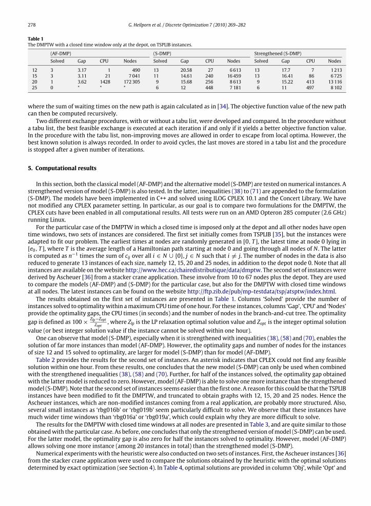
Table 1The DMPTWwith a closed time window only at the depot, on TSPLIB instances.

(AF-DMP) (S-DMP) Strengthened (S-DMP)Solved Gap CPU Nodes Solved Gap CPU Nodes Solved Gap CPU Nodes

12 3 3.17 1 490 13 20.58 27 6613 13 17.7 7 121315 3 3.11 21 7041 11 14.61 240 16459 13 16.41 86 672520 1 3.62 1428 172305 9 15.68 256 8613 9 15.22 413 1311625 0 * * * 6 12 448 7181 6 11 497 8102

where the sum of waiting times on the new path is again calculated as in [34]. The objective function value of the new pathcan then be computed recursively.Two different exchange procedures, with or without a tabu list, were developed and compared. In the procedure without

a tabu list, the best feasible exchange is executed at each iteration if and only if it yields a better objective function value.In the procedure with the tabu list, non-improving moves are allowed in order to escape from local optima. However, thebest known solution is always recorded. In order to avoid cycles, the last moves are stored in a tabu list and the procedureis stopped after a given number of iterations.

5. Computational results

In this section, both the classicalmodel (AF-DMP) and the alternativemodel (S-DMP) are tested on numerical instances. Astrengthened version of model (S-DMP) is also tested. In the latter, inequalities (38) to (71) are appended to the formulation(S-DMP). The models have been implemented in C++ and solved using ILOG CPLEX 10.1 and the Concert Library. We havenot modified any CPLEX parameter setting. In particular, as our goal is to compare two formulations for the DMPTW, theCPLEX cuts have been enabled in all computational results. All tests were run on an AMD Opteron 285 computer (2.6 GHz)running Linux.For the particular case of the DMPTW in which a closed time is imposed only at the depot and all other nodes have open

time windows, two sets of instances are considered. The first set initially comes from TSPLIB [35], but the instances wereadapted to fit our problem. The earliest times at nodes are randomly generated in [0, T ], the latest time at node 0 lying in[e0, T ], where T is the average length of a Hamiltonian path starting at node 0 and going through all nodes of N . The latteris computed as n−1 times the sum of cij over all i ∈ N ∪ {0}, j ∈ N such that i 6= j. The number of nodes in the data is alsoreduced to generate 13 instances of each size, namely 12, 15, 20 and 25 nodes, in addition to the depot node 0. Note that allinstances are available on thewebsite http://www.hec.ca/chairedistributique/data/dmptw. The second set of instanceswerederived by Ascheuer [36] from a stacker crane application. These involve from 10 to 67 nodes plus the depot. They are usedto compare the models (AF-DMP) and (S-DMP) for the particular case, but also for the DMPTW with closed time windowsat all nodes. The latest instances can be found on the website http://ftp.zib.de/pub/mp-testdata/tsp/atsptw/index.html.The results obtained on the first set of instances are presented in Table 1. Columns ‘Solved’ provide the number of

instances solved to optimalitywithin amaximumCPU time of one hour. For these instances, columns ‘Gap’, ‘CPU’ and ‘Nodes’provide the optimality gaps, the CPU times (in seconds) and the number of nodes in the branch-and-cut tree. The optimalitygap is defined as 100× Zlp−Zopt

Zopt, where Zlp is the LP relaxation optimal solution value and Zopt is the integer optimal solution

value (or best integer solution value if the instance cannot be solved within one hour).One can observe that model (S-DMP), especially when it is strengthenedwith inequalities (38), (58) and (70), enables the

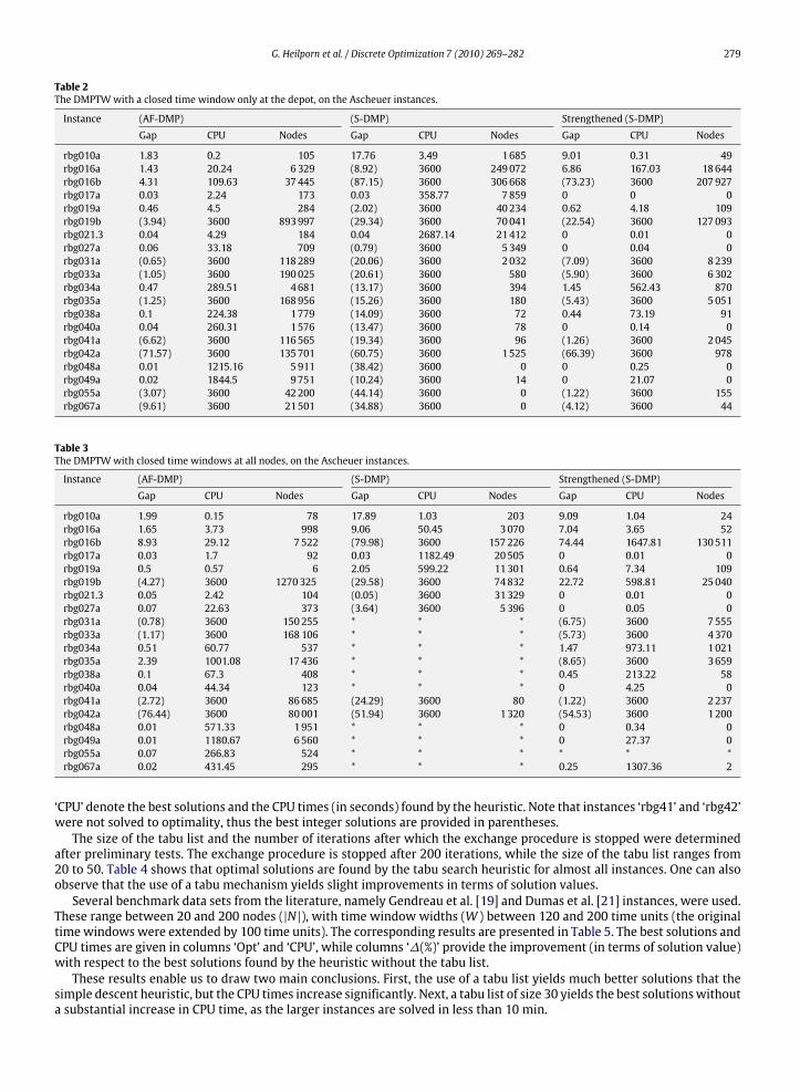
solution of far more instances than model (AF-DMP). However, the optimality gaps and number of nodes for the instancesof size 12 and 15 solved to optimality, are larger for model (S-DMP) than for model (AF-DMP).Table 2 provides the results for the second set of instances. An asterisk indicates that CPLEX could not find any feasible

solution within one hour. From these results, one concludes that the newmodel (S-DMP) can only be used when combinedwith the strengthened inequalities (38), (58) and (70). Further, for half of the instances solved, the optimality gap obtainedwith the lattermodel is reduced to zero. However, model (AF-DMP) is able to solve onemore instance than the strengthenedmodel (S-DMP). Note that the second set of instances seems easier than the first one. A reason for this could be that the TSPLIBinstances have been modified to fit the DMPTW, and truncated to obtain graphs with 12, 15, 20 and 25 nodes. Hence theAscheuer instances, which are non-modified instances coming from a real application, are probably more structured. Also,several small instances as ‘rbg016b’ or ‘rbg019b’ seem particularly difficult to solve. We observe that these instances havemuch wider time windows than ‘rbg016a’ or ‘rbg019a’, which could explain why they are more difficult to solve.The results for the DMPTWwith closed timewindows at all nodes are presented in Table 3, and are quite similar to those

obtainedwith the particular case. As before, one concludes that only the strengthened version ofmodel (S-DMP) can be used.For the latter model, the optimality gap is also zero for half the instances solved to optimality. However, model (AF-DMP)allows solving one more instance (among 20 instances in total) than the strengthened model (S-DMP).Numerical experimentswith the heuristicwere also conducted on two sets of instances. First, the Ascheuer instances [36]

from the stacker crane application were used to compare the solutions obtained by the heuristic with the optimal solutionsdetermined by exact optimization (see Section 4). In Table 4, optimal solutions are provided in column ‘Obj’, while ‘Opt’ and

http://www.hec.ca/chairedistributique/data/dmptw

http://ftp.zib.de/pub/mp-testdata/tsp/atsptw/index.html


Table 2The DMPTWwith a closed time window only at the depot, on the Ascheuer instances.

Instance (AF-DMP) (S-DMP) Strengthened (S-DMP)Gap CPU Nodes Gap CPU Nodes Gap CPU Nodes

rbg010a 1.83 0.2 105 17.76 3.49 1685 9.01 0.31 49rbg016a 1.43 20.24 6329 (8.92) 3600 249072 6.86 167.03 18644rbg016b 4.31 109.63 37445 (87.15) 3600 306668 (73.23) 3600 207927rbg017a 0.03 2.24 173 0.03 358.77 7859 0 0 0rbg019a 0.46 4.5 284 (2.02) 3600 40234 0.62 4.18 109rbg019b (3.94) 3600 893997 (29.34) 3600 70041 (22.54) 3600 127093rbg021.3 0.04 4.29 184 0.04 2687.14 21412 0 0.01 0rbg027a 0.06 33.18 709 (0.79) 3600 5349 0 0.04 0rbg031a (0.65) 3600 118289 (20.06) 3600 2032 (7.09) 3600 8239rbg033a (1.05) 3600 190025 (20.61) 3600 580 (5.90) 3600 6302rbg034a 0.47 289.51 4681 (13.17) 3600 394 1.45 562.43 870rbg035a (1.25) 3600 168956 (15.26) 3600 180 (5.43) 3600 5051rbg038a 0.1 224.38 1779 (14.09) 3600 72 0.44 73.19 91rbg040a 0.04 260.31 1576 (13.47) 3600 78 0 0.14 0rbg041a (6.62) 3600 116565 (19.34) 3600 96 (1.26) 3600 2045rbg042a (71.57) 3600 135701 (60.75) 3600 1525 (66.39) 3600 978rbg048a 0.01 1215.16 5911 (38.42) 3600 0 0 0.25 0rbg049a 0.02 1844.5 9751 (10.24) 3600 14 0 21.07 0rbg055a (3.07) 3600 42200 (44.14) 3600 0 (1.22) 3600 155rbg067a (9.61) 3600 21501 (34.88) 3600 0 (4.12) 3600 44

Table 3The DMPTWwith closed time windows at all nodes, on the Ascheuer instances.

Instance (AF-DMP) (S-DMP) Strengthened (S-DMP)Gap CPU Nodes Gap CPU Nodes Gap CPU Nodes

rbg010a 1.99 0.15 78 17.89 1.03 203 9.09 1.04 24rbg016a 1.65 3.73 998 9.06 50.45 3070 7.04 3.65 52rbg016b 8.93 29.12 7522 (79.98) 3600 157226 74.44 1647.81 130511rbg017a 0.03 1.7 92 0.03 1182.49 20505 0 0.01 0rbg019a 0.5 0.57 6 2.05 599.22 11301 0.64 7.34 109rbg019b (4.27) 3600 1270325 (29.58) 3600 74832 22.72 598.81 25040rbg021.3 0.05 2.42 104 (0.05) 3600 31329 0 0.01 0rbg027a 0.07 22.63 373 (3.64) 3600 5396 0 0.05 0rbg031a (0.78) 3600 150255 * * * (6.75) 3600 7555rbg033a (1.17) 3600 168106 * * * (5.73) 3600 4370rbg034a 0.51 60.77 537 * * * 1.47 973.11 1021rbg035a 2.39 1001.08 17436 * * * (8.65) 3600 3659rbg038a 0.1 67.3 408 * * * 0.45 213.22 58rbg040a 0.04 44.34 123 * * * 0 4.25 0rbg041a (2.72) 3600 86685 (24.29) 3600 80 (1.22) 3600 2237rbg042a (76.44) 3600 80001 (51.94) 3600 1320 (54.53) 3600 1200rbg048a 0.01 571.33 1951 * * * 0 0.34 0rbg049a 0.01 1180.67 6560 * * * 0 27.37 0rbg055a 0.07 266.83 524 * * * * * *rbg067a 0.02 431.45 295 * * * 0.25 1307.36 2

‘CPU’ denote the best solutions and the CPU times (in seconds) found by the heuristic. Note that instances ‘rbg41’ and ‘rbg42’were not solved to optimality, thus the best integer solutions are provided in parentheses.The size of the tabu list and the number of iterations after which the exchange procedure is stopped were determined

after preliminary tests. The exchange procedure is stopped after 200 iterations, while the size of the tabu list ranges from20 to 50. Table 4 shows that optimal solutions are found by the tabu search heuristic for almost all instances. One can alsoobserve that the use of a tabu mechanism yields slight improvements in terms of solution values.Several benchmark data sets from the literature, namely Gendreau et al. [19] and Dumas et al. [21] instances, were used.

These range between 20 and 200 nodes (|N|), with time window widths (W ) between 120 and 200 time units (the originaltime windows were extended by 100 time units). The corresponding results are presented in Table 5. The best solutions andCPU times are given in columns ‘Opt’ and ‘CPU’, while columns ‘∆(%)’ provide the improvement (in terms of solution value)with respect to the best solutions found by the heuristic without the tabu list.These results enable us to draw two main conclusions. First, the use of a tabu list yields much better solutions that the

simple descent heuristic, but the CPU times increase significantly. Next, a tabu list of size 30 yields the best solutionswithouta substantial increase in CPU time, as the larger instances are solved in less than 10 min.


Table 4Heuristic results on the Ascheuer instances.

Instance Without tabu Tabu list of 20 Tabu list of 30 Tabu list of 50|N| Obj Opt CPU Opt CPU Opt CPU Opt CPU

rbg010a 6333 6333 0 6333 0 6333 0 6333 0rbg016a 13705 13705 0 13705 0 13705 1 13705 0rbg016b 5014 5580 0 5014 1 5014 0 5014 0rbg017a 34973 34973 0 34973 0 34973 0 34973 1rbg019a 18947 18947 0 18947 0 18947 1 18947 0rbg019b 10517 10545 0 10545 1 10545 0 10545 1rbg021.3 39699 39699 0 39699 0 39699 0 39699 0rbg027a 67096 67096 0 67096 1 67096 2 67096 2rbg031a 29413 29413 0 29413 2 29413 2 29413 3rbg033a 36914 36914 0 36914 2 36914 2 36914 2rbg034a 41754 41754 0 41754 3 41754 2 41754 3rbg035a 37825 37825 0 37825 2 37825 3 37825 2rbg038a 120752 120752 1 120752 4 120752 3 120752 4rbg040a 118505 118505 0 118505 4 118505 5 118505 6rbg041a (16507) 16532 0 16529 5 16529 4 16529 7rbg042a (7 603) 6 584 1 6107 5 6107 6 5607 6rbg048a 242002 242002 0 242002 6 242002 6 242002 6rbg049a 350832 350832 1 350832 8 350832 7 350832 10rbg055a 191702 191702 1 191702 9 191702 9 191702 12rbg067a 391105 391105 1 391105 17 391105 17 391105 21

Table 5Heuristic results from the Gendreau et al. and Dumas et al. instances.

Instance Without tabu Tabu list of 20 Tabu list of 30 Tabu list of 50|N| W Opt CPU Opt ∆ (%) CPU Opt ∆ (%) CPU Opt ∆ (%) CPU

20 120 2674 0 2567 −3.99 0 2535 −5.19 0 2535 −5.19 120 140 1932 0 1908 −1.23 0 1908 −1.23 0 1908 −1.23 120 160 2190 0 2150 −1.82 0 2149 −1.86 0 2150 −1.82 120 180 2085 0 2046 −1.86 0 2035 −2.39 1 2037 −2.29 120 200 2349 0 2294 −2.33 0 2294 −2.33 1 2294 −2.33 140 120 7535 0 7509 −0.34 3 7509 −0.34 3 7496 −0.51 540 140 7258 0 7205 −0.72 3 7205 −0.72 3 7203 −0.75 440 160 6892 0 6659 −3.37 3 6657 −3.4 3 6657 −3.4 440 180 6966 0 6600 −5.24 3 6583 −5.49 4 6578 −5.56 540 200 6457 0 6408 −0.75 3 6408 −0.75 4 6408 −0.75 560 120 9917 1 9304 −6.17 13 9303 −6.18 15 9303 −6.18 2060 140 9734 1 9131 −6.18 13 9131 −6.18 16 9131 −6.18 2160 160 11454 1 11419 −0.3 10 11422 −0.27 12 11422 −0.27 1760 180 10790 1 9796 −9.2 12 9713 −9.97 14 9689 −10.19 1860 200 10925 1 10758 −1.52 11 10363 −5.13 13 10315 −5.57 1780 120 12150 3 11175 −8.01 31 11122 −8.45 38 11156 −8.17 5280 140 16101 2 14185 −11.89 27 14198 −11.81 33 14131 −12.23 4380 160 9108 3 8614 −5.41 26 8623 −5.31 32 8614 −5.41 4380 180 11625 3 11236 −3.34 33 11226 −3.42 41 11222 −3.46 5680 200 8302 3 8295 −0.07 28 8295 −0.07 34 8272 −0.35 47100 120 22269 6 19351 −13.09 62 19246 −13.56 73 19368 −13.02 94100 140 23351 6 22087 −5.4 60 22078 −5.44 71 22078 −5.44 93100 160 28970 4 27469 −5.17 39 27469 −5.17 46 27368 −5.52 58150 120 28245 35 27816 −1.51 226 27816 −1.51 283 27192 −3.72 388150 140 27768 37 27544 −0.8 225 27382 −1.38 285 27382 −1.38 389150 160 21436 27 20752 −3.18 180 20752 −3.18 226 21123 −1.45 308200 120 18010 44 17886 −0.68 214 17886 −0.68 266 17886 −0.68 356200 140 35203 71 34522 −1.92 434 34410 −2.24 547 34391 −2.3 750

Finally, note that we have also tried to solve the DMPTWby the exact solutionmethodwhile providing the solution of theheuristic as an initial solution. However, this reduces neither the CPU timenor the number of nodes in the branch-and-boundtree.

6. Conclusions

We have studied a variant of the TSPTW with a cumulative objective function, which minimizes the sum of traveldurations between a depot and several locations. Two mixed integer linear programming formulations were proposed forthe problem: a classical arc flow and a sequential assignment model. In order to assess the theoretical strength of the latestmodel, a polyhedral analysis has been performed in the special case where a closed time window is imposed only at the


depot, whereas open time windows are used at all other locations. We have shown that most constraints are facet definingfor the corresponding convex hull of feasible solutions. Next, we have presented both exact and heuristic algorithms forthe problem. Using a general purpose branch-and-cut solver, we were able to solve instances with up to 67 nodes withinreasonable computational times for both models. Whereas the first model solves a fewmore instances than the second one,the latter yields optimality gaps of zero for half of the instances solved to optimality. The heuristic also performs well andprovides good quality solutions, especially when a tabu list is used.

Acknowledgements

Thisworkwas partly funded by the CanadianNatural Sciences and Engineering Research Council under grants 227837-04and 39682-05. This support is gratefully acknowledged. Thanks are due to the referees for their valuable comments.

Appendix. Proof of Lemma 1

Consider that variableswtij : i, j ∈ N, i 6= j, t = 2, . . . , n are sorted by lexicographic order on (t, i, j). Furthermore, for alli, j ∈ N (i 6= j), let π i and π ij denote permutations of the nodes in N \ {i, n− 1, n} and N \ {i, j, n− 1, n}, respectively. Thenotations π ijS and π

ijS̄represent node permutations in the complementary subsets S and S̄, where S ∪ S̄ = N \ {i, j, n− 1, n}.

One can check that the following combinations of rows of the path-w matrix are affinely independent:

f 2,i,n = (0, i, n, n− 1, π i)− (0, n, i, n− 1, π i)= w2in − w

2ni + w

3n(n−1) − w

3i(n−1) i ∈ N \ {n− 1, n} (81)

f 2,n−1,n = (0, n− 1, n, n− 2, πn−2)− (0, n, n− 1, n− 2, πn−2)= w2(n−1)n − w

2n(n−1) + w

3n(n−2) − w

3(n−1)(n−2) (82)

f t,i,j = (0, π ijS , i, j, n, n− 1, πijS̄)− (0, π ijS , i, n, j, n− 1, π

ijS̄)

= wtij − wtin + w

t+1jn − w

t+1nj + w

t+2n(n−1) − w

t+2j(n−1) t = 2, . . . n− 1, i, j ∈ N \ {n− 1, n} : i 6= j (83)

f t,i,n−1 = (0, π i(n−2)S , i, n− 1, n, n− 2, π i(n−2)S̄

)− (0, π i(n−2)S , i, n, n− 1, n− 2, π i(n−2)S̄

)

= wti(n−1) − wtin + w

t+1(n−1)n − w

t+1n(n−1) + w

t+2n(n−2) − w

t+2(n−1)(n−2)

t = 2, . . . , n− 1, i ∈ N \ {n− 2, n− 1, n} (84)

f t,n−2,n−1 = (0, π (n−2)(n−3)S , n− 2, n− 1, n, n− 3, π (n−2)(n−3)S̄

)

− (0, π (n−2)(n−3)S , n− 2, n, n− 1, n− 3, π (n−2)(n−3)S̄

)

= wt(n−2)(n−1) − wt(n−2)n + w

t+1(n−1)n − w

t+1n(n−1) + w

t+2n(n−3) − w

t+2(n−1)(n−3) t = 2, . . . , n− 1 (85)

f t,n−1,i = (0, π i(n−2)S , n− 1, i, n, n− 2, π i(n−2)S̄

)− (0, π i(n−2)S , n− 1, n, i, n− 2, π i(n−2)S̄

)

= wt(n−1)i − wt(n−1)n + w

t+1in − w

t+1ni + w

t+2n(n−2) − w

t+2i(n−2) t = 2, . . . , n− 1, i ∈ N \ {n− 2, n− 1, n} (86)

f t,n−1,n−2 = (0, π (n−2)(n−3)S , n− 1, n− 2, n, n− 3, π (n−2)(n−3)S̄

)

− (0, π (n−2)(n−3)S , n− 1, n, n− 2, n− 3, π (n−2)(n−3)S̄

)

= wt(n−1)(n−2) − wt(n−1)n + w

t+1(n−2)n − w

t+1n(n−2) + w

t+2n(n−3) − w

t+2(n−2)(n−3) t = 2, . . . , n− 1 (87)

f t,n,i = (0, π i(n−2)S , n, i, n− 1, n− 2, π i(n−2)S̄

)− (0, π i(n−2)S , n, n− 1, i, n− 2, π i(n−2)S̄

)

= wtni − wtn(n−1) + w

t+1i(n−1) − w

t+1(n−1)i + w

t+2(n−1)(n−2) − w

t+2i(n−2) t = 2, . . . , n− 1, i ∈ N \ {n− 2, n− 1, n} (88)

f t,n,n−2 = (0, π (n−2)(n−3)S , n, n− 2, n− 1, n− 3, π (n−2)(n−3)S̄

)

− (0, π (n−2)(n−3)S , n, n− 1, n− 2, n− 3, π (n−2)(n−3)S̄

)

= wtn(n−2) − wtn(n−1) + w

t+1(n−2)(n−1) − w

t+1(n−1)(n−2) + w

t+2(n−1)(n−3) − w

t+2(n−2)(n−3) t = 2, . . . , n− 1 (89)

f n,i,j = (0, π ij, n, n− 1, i, j)− (0, π ij, n, i, j, n− 1)= wn−2n(n−1) − w

n−2ni + w

n−1(n−1)i − w

n−1ij + w

nij − w

nj(n−1) i, j ∈ N \ {n− 1, n} : i 6= j (90)

f n,i,n−1 = (0, π i(n−2), n− 2, n, i, n− 1)− (0, π i(n−2), n− 2, n− 1, i, n)= wn−2(n−2)n − w

n−2(n−2)(n−1) + w

n−1ni − w

n−1(n−1)i + w

ni(n−1) − w

nin i ∈ N \ {n− 2, n− 1, n} (91)


f n,n−2,n−1 = (0, π (n−3)(n−2), n− 3, n, n− 2, n− 1)− (0, π (n−3)(n−2), n− 3, n− 1, n− 2, n)= wn−2(n−3)n − w

n−2(n−3)(n−1) + w

n−1n(n−2) − w

n−1(n−1)(n−2) + w

n(n−2)(n−1) − w

n(n−2)n (92)

f n,n−1,i = (0, π i(n−2), n− 2, n, n− 1, i)− (0, π i(n−2), n− 2, i, n− 1, n)= wn−2(n−2)n − w

n−2(n−2)i + w

n−1n(n−1) − w

n−1i(n−1) + w

n(n−1)i − w

n(n−1)n i ∈ N \ {n− 2, n− 1, n}. (93)

Combinations (81)–(89) form an upper triangular matrix with unit determinant and are thus affinely independent. One canalso check that (90)–(93) are affinely independent from all other combinations. Indeed, each combination (90) containstermswn−1ij ,w

nij and now

njn norw

nnj, (91) (resp. (92)) contain termsw

ni(n−1),w

nin and now

nn(n−1),w

n(n−1)n norw

n(n−1)i (resp. the

same terms with i = n− 2), while (93) contains termswn(n−1)i,wn(n−1)n and now

nn(n−1) norw

ni(n−1).

There are n−1 combinations of class f 2,i,n or f 2,n−1,n, (n−2)2(n−3) combinations of class f t,i,j, and 3(n−2)2 combinationsamong the classes f t,i,n−1, f t,n−2,n−1, f t,n−1,i, f t,n−1,n−2, f t,n,i or f t,n,n−2. Further, there are (n − 2)(n − 3) combinations ofclass f n,i,j and 2n− 5 combinations among the classes f n,i,n−1, f n,n−2,n−1 and f n,n−1,i. The result follows. �

References

[1] F. Li, B.L. Golden, E.A. Wasil, The open vehicle routing problem: algorithms, large-scale test problems, and computational results, Computers &Operations Research 34 (2007) 2918–2930.

[2] A.N. Letchford, J. Lysgaard, R.W. Eglese, A branch-and-cut algorithm for the capacitated open vehicle routing problem, Journal of the OperationalResearch Society 58 (2007) 1642–1651.

[3] P.P. Repoussis, C.D. Tarantilis, G. Ioannou, The open vehicle routing problemwith timewindows, Journal of the Operational Research Society 58 (2007)355–367.

[4] J.N. Tsitsiklis, Special cases of traveling salesman and repairman problems with time windows, Networks 22 (1992) 263–283.[5] A. Lucena, Time-dependent traveling salesman problem — the deliveryman case, Networks 20 (1990) 753–763.[6] M. Fischetti, G. Laporte, S. Martello, The delivery man problem and cumulative matroids, Operations Research 41 (1993) 1055–1064.[7] C.A. van Eijl, A polyhedral approach to the delivery man problem. Technical Report Memorandum COSOR 95-19, Eindhoven University of Technology,The Netherlands, 1995.

[8] I. Méndez-Díaz, P. Zabala, A. Lucena, A new formulation for the traveling deliveryman problem, Discrete AppliedMathematics 156 (2008) 3223–3237.[9] A. Blum, P. Chalasani, D. Coppersmith, B. Pulleyblank, P. Raghavan, M. Sudan, The minimum latency problem, in: Proceedings of the 26th ACMSymposium on the Theory of Computing, 1994, pp. 163–171.

[10] M. Goemans, J. Kleinberg, An improved approximation ratio for the minimum latency problem, Mathematical Programming 82 (1998) 114–124.[11] K. Chaudhuri, B. Godfrey, S. Rao, K. Talwar, Paths, trees and minimum latency tours, in: Proceedings of the 44th Symposium on Foundations of

Computer Science, 2003, pp. 36–45.[12] B.Y. Wu, Z.N. Huang, F.J. Zhan, Exact algorithms for the minimum latency problem, Information Processing Letters 92 (2004) 303–309.[13] E.K. Baker, An exact algorithm for the time-constrained traveling salesman problem, Operations Research 31 (1983) 938–945.[14] A. Langevin, M. Desrochers, J. Desrosiers, S. Gélinas, F. Soumis, A two-commodity flow formulation for the traveling salesman andmakespan problems

with time windows, Networks 23 (1993) 631–640.[15] N. Ascheuer, M. Fischetti, M. Grötschel, A polyhedral study of the asymmetric travelling salesman problem with time windows, Mathematical

Programming Series A 90 (2000) 475–506.[16] N. Ascheuer, M. Fischetti, M. Grötschel, Solving the asymmetric travelling salesman problem with time windows by branch-and-cut, Networks 36

(2000) 69–79.[17] V. Mak, A.T. Ernst, New cutting-planes for the time and/or precedence constrained ATSP and directed VRP, Mathematical Methods of Operations

Research 66 (2007) 69–98.[18] L. Bianco, A. Mingozzi, S. Ricciardelli, The traveling salesman problem with cumulative costs, Networks 23 (1993) 81–91.[19] M. Gendreau, A. Hertz, G. Laporte, M. Stan, A generalized insertion heuristic for the traveling salesman problem with time windows, Operations

Research 43 (1998) 330–335.[20] R. Wolfler Calvo, A new heuristic for the traveling salesman problem with time windows, Transportation Science 34 (2000) 113–124.[21] Y. Dumas, J. Desrosiers, E. Gélinas, An optimal algorithm for the traveling salesman problem with time windows, Operations Research 43 (1995)

367–371.[22] L. Bianco, A. Mingozzi, S. Ricciardelli, Dynamic programming strateges and reduction techniques for the travelling salesman problem with time

windows and precedence constraints, Operations Research 45 (1997) 365–377.[23] G. Pesant, M. Gendreau, J.-Y. Potvin, J.-M. Rousseau, An exact constraint logic programming algorithm for the traveling salesman problem with time

windows, Transportation Science 32 (1998) 12–29.[24] F. Focacci, A. Lodi, M. Milano, A hybrid exact algorithm for the TSPTW, INFORMS Journal on Computing 14 (2002) 403–417.[25] M.W.P. Savelsbergh, Local search for routing problems with time windows, Annals of Operations Research 4 (1985) 285–305.[26] T. Öncan, I.K. Altinel, G. Laporte, A comparative analysis of several asymmetric traveling salesman problem formulations, Computers & Operations

Research 36 (2009) 637–654.[27] L. Gouveia, J.M. Pires, The asymmetric traveling salesman problem: on generalizations of disaggregated Miller–Tucker–Zemlin constraints, Discrete

Applied Mathematics 112 (2001) 129–145.[28] J.-C. Picard, M. Queyranne, The time-dependent traveling salesman problem and its application to the tardiness problem in one-machine scheduling,

Operations Research 26 (1978) 86–110.[29] K.R. Fox, B. Gavish, S.C. Graves, An n-constraint formulation of the (time-dependent) traveling salesman problem, Operations Research 28 (1980)

1018–1021.[30] L.-P. Bigras, M. Gamache, G. Savard, The time-dependent traveling salesman problem and single machine scheduling problems with sequence

dependent setup times, Discrete Optimization 5 (2008) 685–699.[31] M. Queyranne, A.S. Schulz, Polyhedral approaches to machine scheduling. Technical Report 408, Department of Mathematics, Technical University of

Berlin, 1994.[32] A.B. Keha, K. Khowala, J.W. Fowler, Mixed integer programming formulations for single machine scheduling problems, Computers & Operations

Research 36 (2009) 2122–2131.[33] H. Abeledo, A. Pessoa, E. Uchoa, A polyhedral study of the time-dependent traveling salesman problem, in: Proceedings of the VI ALIO/EUROWorkshop

on Applied Combinatorial Optimization, 2008, pp. 1–6.[34] M.W.P. Savelsbergh, The vehicle routing problem with time windows: minimizing route duration, ORSA Journal on Computing 4 (1992) 146–154.[35] G. Reinelt, TSPLIB A traveling salesman problem library, ORSA Journal on Computing 3 (1991) 376–384.[36] N. Ascheuer, Hamiltonian path problems in the online optimization of flexible manufacturing systems. Ph.D. Thesis, Technische Universität Berlin,

1995.

Documents

The Delivery Man Problem With Time Windows