The Economics of Density:

Evidence from the Berlin Wall

Gabriel M. AhlfeldtLondon School of Economics and CEPR

Stephen J. ReddingPrinceton University, NBER and CEPR

Daniel M. SturmLondon School of Economics and CEPR

Nikolaus WolfHumboldt University and CEPR

1 / 40

Motivation

• Economic activity is highly unevenly distributed across space:– The existence of cities (e.g. 19 cities worldwide had a population

greater than 10 million in 2007)

– Concentrations of economic functions within cities (e.g. advertising

agencies in mid-town Manhattan)

• A key research objective is determining the strength ofagglomeration and dispersion forces

– Agglomeration: increasing returns

– Dispersion: land scarcity and commuting costs

• Determining the magnitude of these forces is central to a host ofeconomic and policy issues:

– Productivity advantages of cities

– Cost-benefit analyzes of transport infrastructure

– E↵ects of property taxation and regional policy

2 / 40

Empirical Challenges

• Economic activities often cluster together because of sharedlocational fundamentals

– What are the roles of agglomeration/dispersion forces versus shared

natural advantages?

– Historical natural advantages can have long-lived e↵ects through for

example sunk costs or coordination e↵ects

• One approach regresses productivity, wages or employment on thedensity of economic activity

– Third variables can a↵ect both productivity and wages and density

– Di�cult to find instruments that only a↵ect productivity or wages

through density (with a few exceptions)

• Little evidence on the spatial scale of agglomeration forces orseparating them from congestion forces

• Di�cult to find sources of exogenous variation in the surroundingconcentration of economic activity

3 / 40

This Paper

• We develop a quantitative model of city structure to determineagglomeration and dispersion forces, while also allowingempirically-relevant variation in:

– Production locational fundamentals

– Residential locational fundamentals

– Transportation infrastructure

• We combine the model with data for thousands of city blocks inBerlin in 1936, 1986 and 2006 on:

– Land prices

– Workplace employment

– Residence employment

• We use the division of Berlin in the aftermath of the Second WorldWar and its reunification in 1989 as a source of exogenous variationin the surrounding concentration of economic activity

4 / 40

Road Map

• Historical Background

• Theoretical Model

• Data

• Reduced-Form Evidence

• Structural Estimation

5 / 40

Historical Background

• A protocol signed during the Second World War organized Germanyinto American, British, French and Soviet occupation zones

• Although 200km within the Soviet zone, Berlin was to be jointlyoccupied and organized into four occupation sectors:

– Boundaries followed pre-war district boundaries, with the same

East-West orientation as the occupation zones, and created sectors

of roughly equal pre-war population (prior to French sector)

– Protocol envisioned a joint city administration (“Kommandatura”)

• Following the onset of the Cold War– East and West Germany founded as separate states and separate city

governments created in East and West Berlin in 1949

– The adoption of Soviet-style policies of command and control in East

Berlin limited economic interactions with West Berlin

– To stop civilians leaving for West Germany, the East German

authorities constructed the Berlin Wall in 1961

6 / 40

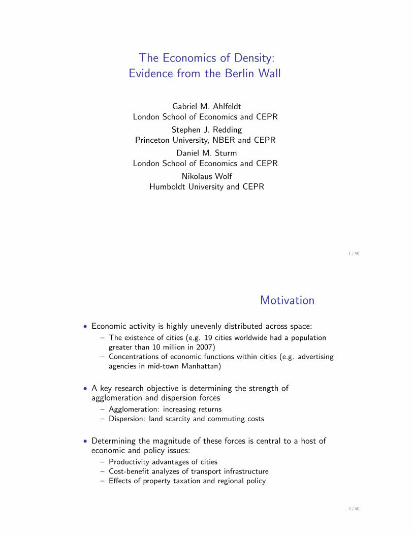
The Division of Berlin

7 / 40

Theoretical Framework

• We build on the urban model of Lucas and Rossi-Hansberg (2002),which has a number of attractive features

– Models city structure in continuous two-dimensional space

– Does not impose mono-centricity

– But considers a symmetric circular city

• We develop an empirically-tractable version of this model– Model the city as a large number of discrete blocks

– Allow for di↵erences in production fundamentals, residential

fundamentals and transport connections across blocks

– As a result the model allows for a rich asymmetric distribution of

economic activity within the city

• The model remains tractable because of heterogeneity in workers’commuting decisions, modeled following Eaton and Kortum (2002)

• The model provides a quantitative framework that can also be usedfor analyzing other interventions (e.g. transport network)

8 / 40

Model Setup

• We consider a city embedded within a larger economy, whichprovides a reservation level of utility (U)

• The city consists of a set of discrete blocks indexed by i , with supplyof floor space depending on the density of development (ji )

• There is a single final good which is costlessly traded and is chosenas the numeraire

• Markets are perfectly competitive

• Workers choose a block of residence, a block of employment, andconsumption of the final good and floor space to max utility

• Firms choose a block of production and inputs of labor and floorspace to max profits

• Floor space within each block optimally allocated betweenresidential and commercial use

• Productivity depends on fundamentals (ai ) & spillovers (Ui )

• Amenities depend on fundamentals (bi ) & spillovers (Wi )

• Workers face commuting costs

9 / 40

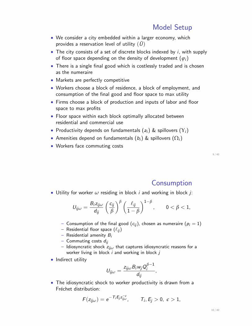
Consumption

• Utility for worker w residing in block i and working in block j :

Uijw =Bizijw

dij

✓cij

b

◆b ✓ `ij1� b

◆1�b

, 0 < b < 1,

– Consumption of the final good (cij ), chosen as numeraire (pi = 1)

– Residential floor space (`ij )– Residential amenity Bi

– Commuting costs dij– Idiosyncratic shock zijw that captures idiosyncratic reasons for a

worker living in block i and working in block j

• Indirect utility

Uijw =zijwBiwjQ

b�1i

dij,

• The idiosyncratic shock to worker productivity is drawn from aFrechet distribution:

F (zijw) = e�TiEj z

�eijw , Ti ,Ej > 0, e > 1,

10 / 40

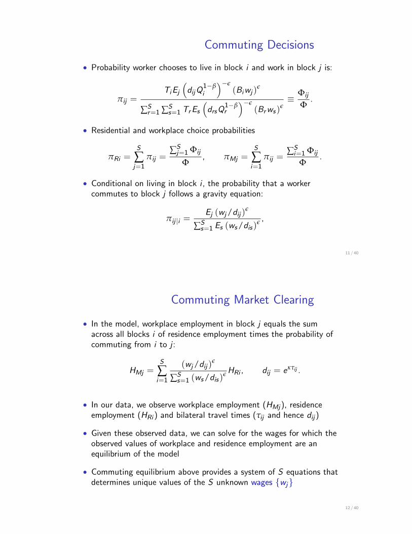
Commuting Decisions

• Probability worker chooses to live in block i and work in block j is:

pij =TiEj

⇣dijQ

1�bi

⌘�e(Biwj )

e

ÂS

r=1 ÂS

s=1 TrEs

⇣drsQ

1�br

⌘�e(Brws)

e⌘ Fij

F.

• Residential and workplace choice probabilities

pRi =S

Âj=1

pij =ÂS

j=1 Fij

F, pMj =

S

Âi=1

pij =ÂS

i=1 Fij

F.

• Conditional on living in block i , the probability that a workercommutes to block j follows a gravity equation:

pij |i =Ej (wj/dij )

e

ÂS

s=1 Es (ws/dis)e ,

11 / 40

Commuting Market Clearing

• In the model, workplace employment in block j equals the sumacross all blocks i of residence employment times the probability ofcommuting from i to j :

HMj =S

Âi=1

(wj/dij )e

ÂS

s=1 (ws/dis)e HRi , dij = e

ktij .

• In our data, we observe workplace employment (HMj ), residenceemployment (HRi ) and bilateral travel times (tij and hence dij )

• Given these observed data, we can solve for the wages for which theobserved values of workplace and residence employment are anequilibrium of the model

• Commuting equilibrium above provides a system of S equations thatdetermines unique values of the S unknown wages {wj}

12 / 40

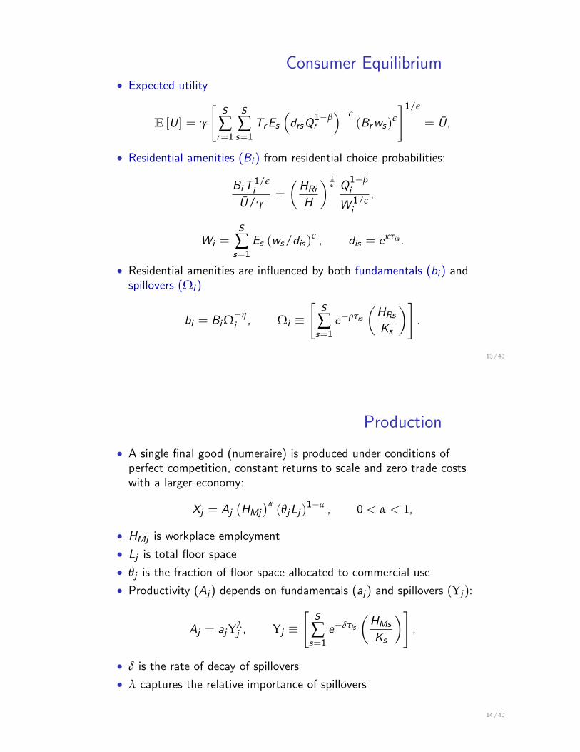
Consumer Equilibrium

• Expected utility

E [U ] = g

"S

Âr=1

S

Âs=1

TrEs

⇣drsQ

1�br

⌘�e(Brws)

e

#1/e

= U,

• Residential amenities (Bi ) from residential choice probabilities:

BiT1/ei

U/g=

✓HRi

H

◆ 1e Q

1�bi

W1/ei

,

Wi =S

Âs=1

Es (ws/dis)e , dis = e

ktis .

• Residential amenities are influenced by both fundamentals (bi ) andspillovers (Wi )

bi = BiW�hi

, Wi ⌘"

S

Âs=1

e�rtis

✓HRs

Ks

◆#.

13 / 40

Production

• A single final good (numeraire) is produced under conditions ofperfect competition, constant returns to scale and zero trade costswith a larger economy:

Xj = Aj

�HMj

�a(qjLj )

1�a , 0 < a < 1,

• HMj is workplace employment

• Lj is total floor space

• qj is the fraction of floor space allocated to commercial use

• Productivity (Aj ) depends on fundamentals (aj ) and spillovers (Uj ):

Aj = ajUlj, Uj ⌘

"S

Âs=1

e�dtis

✓HMs

Ks

◆#,

• d is the rate of decay of spillovers

• l captures the relative importance of spillovers

14 / 40

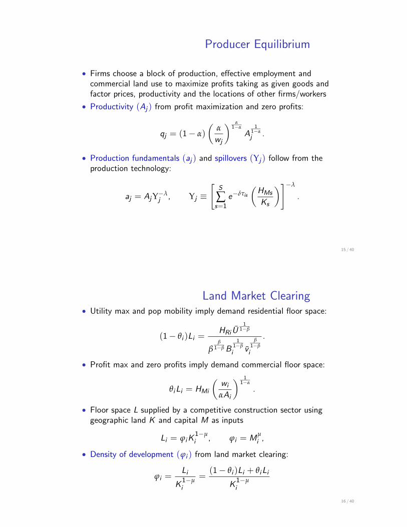
Producer Equilibrium

• Firms choose a block of production, e↵ective employment andcommercial land use to maximize profits taking as given goods andfactor prices, productivity and the locations of other firms/workers

• Productivity (Aj ) from profit maximization and zero profits:

qj = (1� a)

✓a

wj

◆ a1�a

A

11�aj

.

• Production fundamentals (aj ) and spillovers (Uj ) follow from theproduction technology:

aj = AjU�lj

, Uj ⌘"

S

Âs=1

e�dtis

✓HMs

Ks

◆#�l

.

15 / 40

Land Market Clearing

• Utility max and pop mobility imply demand residential floor space:

(1� qi )Li =HRi U

11�b

bb

1�b B

11�b

iv

b1�b

i

.

• Profit max and zero profits imply demand commercial floor space:

qiLi = HMi

✓wi

aAi

◆ 11�a

.

• Floor space L supplied by a competitive construction sector usinggeographic land K and capital M as inputs

Li = jiK1�µi

, ji = Mµi,

• Density of development (ji ) from land market clearing:

ji =Li

K1�µi

=(1� qi )Li + qiLi

K1�µi

16 / 40

Qualitative Predictions for Division

• Firms in West Berlin cease to benefit from production externalitiesfrom employment centers in East Berlin

– Reduces productivity, land prices and employment

• Firms in West Berlin lose access to flows of commuters fromresidential concentrations in East Berlin

– Increases the wage required to achieve a given e↵ective employment,

reducing land prices and employment

• Residents in West Berlin lose access to employment opportunitiesand consumption externalities from East Berlin

– Reduces expected worker income, land prices and residents

• The impact is greater for parts of West Berlin closer to employmentand residential concentrations in East Berlin

• Employment and residents reallocate within West Berlin and thelarger economy until wages and land prices adjust such that:

– Firms make zero profits in each location with positive production

– Workers are indi↵erent across all locations with positive residents

– No-arbitrage between commercial and residential land use

17 / 40

Data

• Data on land prices, workplace employment, residence employmentand bilateral travel times

• Data for Greater Berlin in 1936 and 2006

• Data for West Berlin in 1986

• Data at the following levels of spatial aggregation:– Pre-war districts (“Bezirke”), 20 in Greater Berlin, 12 in West Berlin

– Statistical areas (“Gebiete”), around 90 in West Berlin

– Statistical blocks, around 9,000 in West Berlin

• Land prices: o�cial assessed land value of a representativeundeveloped property or the fair market value of a developedproperty if it were not developed

• Geographical Information Systems (GIS) data on:– land area, land use, building density, proximity to U-Bahn

(underground) and S-Bahn (suburban) stations, schools, parks, lakes,

canals and rivers, Second World War destruction, location of

government buildings and urban regeneration programs

18 / 40

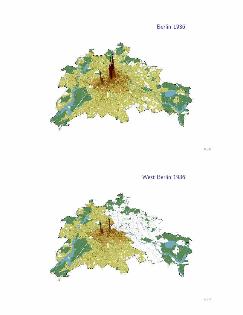
Berlin 1936

19 / 40

West Berlin 1936

20 / 40

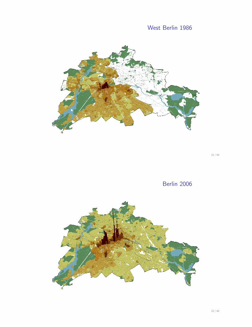
West Berlin 1986

21 / 40

Berlin 2006

22 / 40

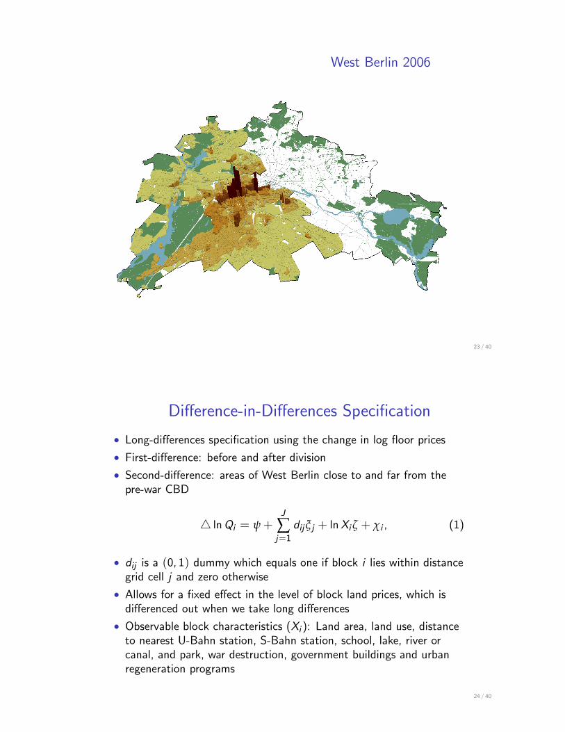
West Berlin 2006

23 / 40

Di↵erence-in-Di↵erences Specification

• Long-di↵erences specification using the change in log floor prices

• First-di↵erence: before and after division

• Second-di↵erence: areas of West Berlin close to and far from thepre-war CBD

4 lnQi = y +J

Âj=1

dijxj + lnXi z + ci , (1)

• dij is a (0, 1) dummy which equals one if block i lies within distancegrid cell j and zero otherwise

• Allows for a fixed e↵ect in the level of block land prices, which isdi↵erenced out when we take long di↵erences

• Observable block characteristics (Xi ): Land area, land use, distanceto nearest U-Bahn station, S-Bahn station, school, lake, river orcanal, and park, war destruction, government buildings and urbanregeneration programs

24 / 40

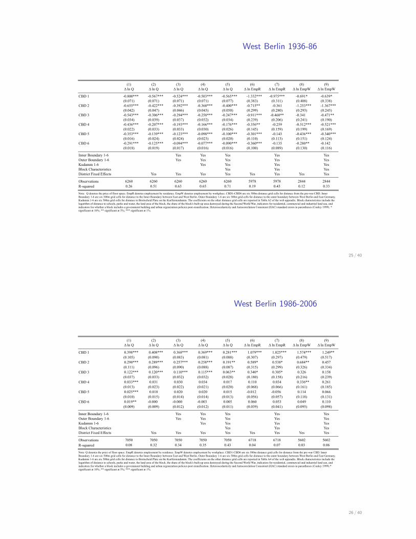
West Berlin 1936-86

(1) (2) (3) (4) (5) (6) (7) (8) (9)Δ ln Q Δ ln Q Δ ln Q Δ ln Q Δ ln Q Δ ln EmpR Δ ln EmpR Δ ln EmpW Δ ln EmpW

CBD 1 -0.800*** -0.567*** -0.524*** -0.503*** -0.565*** -1.332*** -0.975*** -0.691* -0.639*(0.071) (0.071) (0.071) (0.071) (0.077) (0.383) (0.311) (0.408) (0.338)

CBD 2 -0.655*** -0.422*** -0.392*** -0.360*** -0.400*** -0.715** -0.361 -1.253*** -1.367***(0.042) (0.047) (0.046) (0.043) (0.050) (0.299) (0.280) (0.293) (0.243)

CBD 3 -0.543*** -0.306*** -0.294*** -0.258*** -0.247*** -0.911*** -0.460** -0.341 -0.471**(0.034) (0.039) (0.037) (0.032) (0.034) (0.239) (0.206) (0.241) (0.190)

CBD 4 -0.436*** -0.207*** -0.193*** -0.166*** -0.176*** -0.356** -0.259 -0.512*** -0.521***(0.022) (0.033) (0.033) (0.030) (0.026) (0.145) (0.159) (0.199) (0.169)

CBD 5 -0.353*** -0.139*** -0.123*** -0.098*** -0.100*** -0.301*** -0.143 -0.436*** -0.340***(0.016) (0.024) (0.024) (0.023) (0.020) (0.110) (0.113) (0.151) (0.124)

CBD 6 -0.291*** -0.125*** -0.094*** -0.077*** -0.090*** -0.360*** -0.135 -0.280** -0.142 (0.018) (0.019) (0.017) (0.016) (0.016) (0.100) (0.089) (0.130) (0.116)

Inner Boundary 1-6 Yes Yes Yes Yes YesOuter Boundary 1-6 Yes Yes Yes Yes YesKudamm 1-6 Yes Yes Yes YesBlock Characteristics Yes Yes YesDistrict Fixed Effects Yes Yes Yes Yes Yes Yes Yes Yes

Observations 6260 6260 6260 6260 6260 5978 5978 2844 2844R-squared 0.26 0.51 0.63 0.65 0.71 0.19 0.43 0.12 0.33

Note: Q denotes the price of floor space. EmpR denotes employment by residence. EmpW denotes employment by workplace. CBD1-CBD6 are six 500m distance grid cells for distance from the pre-war CBD. Inner Boundary 1-6 are six 500m grid cells for distance to the Inner Boundary between East and West Berlin. Outer Boundary 1-6 are six 500m grid cells for distance to the outer boundary between West Berlin and East Germany. Kudamm 1-6 are six 500m grid cells for distance to Breitscheid Platz on the Kurfürstendamm. The coefficients on the other distance grid cells are reported in Table A2 of the web appendix. Block characteristics include the logarithm of distance to schools, parks and water, the land area of the block, the share of the block's built-up area destroyed during the Second World War, indicators for residential, commercial and industrial land use, and indicators for whether a block includes a government building and urban regeneration policies post-reunification. Heteroscedasticity and Autocorrelation Consistent (HAC) standard errors in parentheses (Conley 1999). * significant at 10%; ** significant at 5%; *** significant at 1%.

25 / 40

West Berlin 1986-2006

(1) (2) (3) (4) (5) (6) (7) (8) (9)Δ ln Q Δ ln Q Δ ln Q Δ ln Q Δ ln Q Δ ln EmpR Δ ln EmpR Δ ln EmpW Δ ln EmpW

CBD 1 0.398*** 0.408*** 0.368*** 0.369*** 0.281*** 1.079*** 1.025*** 1.574*** 1.249**(0.105) (0.090) (0.083) (0.081) (0.088) (0.307) (0.297) (0.479) (0.517)

CBD 2 0.290*** 0.289*** 0.257*** 0.258*** 0.191** 0.589* 0.538* 0.684** 0.457(0.111) (0.096) (0.090) (0.088) (0.087) (0.315) (0.299) (0.326) (0.334)

CBD 3 0.122*** 0.120*** 0.110*** 0.115*** 0.063** 0.340* 0.305* 0.326 0.158(0.037) (0.033) (0.032) (0.032) (0.028) (0.180) (0.158) (0.216) (0.239)

CBD 4 0.033*** 0.031 0.030 0.034 0.017 0.110 0.034 0.336** 0.261(0.013) (0.023) (0.022) (0.021) (0.020) (0.068) (0.066) (0.161) (0.185)

CBD 5 0.025*** 0.018 0.020 0.020 0.015 -0.012 -0.056 0.114 0.066(0.010) (0.015) (0.014) (0.014) (0.013) (0.056) (0.057) (0.118) (0.131)

CBD 6 0.019** -0.000 -0.000 -0.003 0.005 0.060 0.053 0.049 0.110(0.009) (0.009) (0.012) (0.012) (0.011) (0.039) (0.041) (0.095) (0.098)

Inner Boundary 1-6 Yes Yes Yes Yes YesOuter Boundary 1-6 Yes Yes Yes Yes YesKudamm 1-6 Yes Yes Yes YesBlock Characteristics Yes Yes YesDistrict Fixed Effects Yes Yes Yes Yes Yes Yes Yes Yes

Observations 7050 7050 7050 7050 7050 6718 6718 5602 5602R-squared 0.08 0.32 0.34 0.35 0.43 0.04 0.07 0.03 0.06

Note: Q denotes the price of floor space. EmpR denotes employment by residence. EmpW denotes employment by workplace. CBD1-CBD6 are six 500m distance grid cells for distance from the pre-war CBD. Inner Boundary 1-6 are six 500m grid cells for distance to the Inner Boundary between East and West Berlin. Outer Boundary 1-6 are six 500m grid cells for distance to the outer boundary between West Berlin and East Germany. Kudamm 1-6 are six 500m grid cells for distance to Breitscheid Platz on the Kurfürstendamm. The coefficients on the other distance grid cells are reported in Table A4 of the web appendix. Block characteristics include the logarithm of distance to schools, parks and water, the land area of the block, the share of the block's built-up area destroyed during the Second World War, indicators for residential, commercial and industrial land use, and indicators for whether a block includes a government building and urban regeneration policies post-reunification. Heteroscedasticity and Autocorrelation Consistent (HAC) standard errors in parentheses (Conley 1999).* significant at 10%; ** significant at 5%; *** significant at 1%.

26 / 40

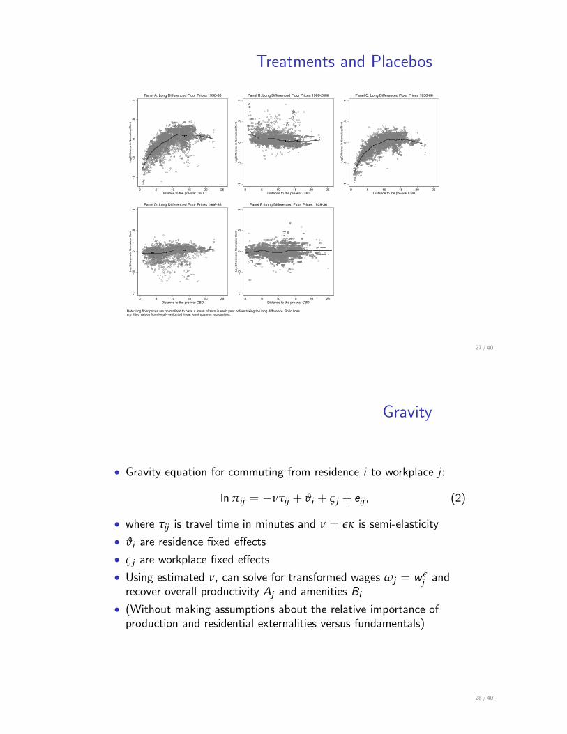
Treatments and Placebos

-1-.5

0.5

1Lo

g D

iffer

ence

in N

orm

aliz

ed R

ent

0 5 10 15 20 25Distance to the pre-war CBD

Panel A: Long Differenced Floor Prices 1936-86

-1-.5

0.5

1Lo

g D

iffer

ence

in N

orm

aliz

ed R

ent

0 5 10 15 20 25Distance to the pre-war CBD

Panel B: Long Differenced Floor Prices 1986-2006

-1-.5

0.5

1Lo

g D

iffer

ence

in N

orm

aliz

ed R

ent

0 5 10 15 20 25Distance to the pre-war CBD

Panel C: Long Differenced Floor Prices 1936-66

-1-.5

0.5

1Lo

g D

iffer

ence

in N

orm

aliz

ed R

ent

0 5 10 15 20 25Distance to the pre-war CBD

Panel D: Long Differenced Floor Prices 1966-86

-1-.5

0.5

1Lo

g D

iffer

ence

in N

orm

aliz

ed R

ent

0 5 10 15 20 25Distance to the pre-war CBD

Panel E: Long Differenced Floor Prices 1928-36

Note: Log floor prices are normalized to have a mean of zero in each year before taking the long difference. Solid linesare fitted values from locally-weighted linear least squares regressions.

27 / 40

Gravity

• Gravity equation for commuting from residence i to workplace j :

lnpij = �ntij + Ji + Vj + eij , (2)

• where tij is travel time in minutes and n = ek is semi-elasticity

• Ji are residence fixed e↵ects

• Vj are workplace fixed e↵ects

• Using estimated n, can solve for transformed wages wj = wejand

recover overall productivity Aj and amenities Bi

• (Without making assumptions about the relative importance ofproduction and residential externalities versus fundamentals)

28 / 40

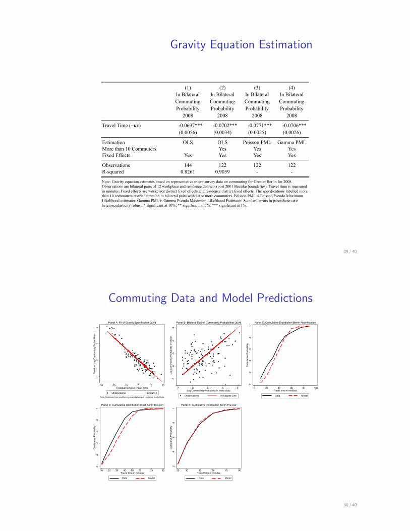
Gravity Equation Estimation

(1) (2) (3) (4)ln Bilateral Commuting Probability

2008

ln Bilateral Commuting Probability

2008

ln Bilateral Commuting Probability

2008

ln Bilateral Commuting Probability

2008

Travel Time (−κε) -0.0697*** -0.0702*** -0.0771*** -0.0706***(0.0056) (0.0034) (0.0025) (0.0026)

Estimation OLS OLS Poisson PML Gamma PMLMore than 10 Commuters Yes Yes YesFixed Effects Yes Yes Yes Yes

Observations 144 122 122 122R-squared 0.8261 0.9059 - -

Note: Gravity equation estimates based on representative micro survey data on commuting for Greater Berlin for 2008. Observations are bilateral pairs of 12 workplace and residence districts (post 2001 Bezirke boundaries). Travel time is measured in minutes. Fixed effects are workplace district fixed effects and residence district fixed effects. The specifications labelled more than 10 commuters restrict attention to bilateral pairs with 10 or more commuters. Poisson PML is Poisson Pseudo Maximum Likelihood estimator. Gamma PML is Gamma Pseudo Maximum Likelihood Estimator. Standard errors in parentheses are heteroscedasticity robust. * significant at 10%; ** significant at 5%; *** significant at 1%.

29 / 40

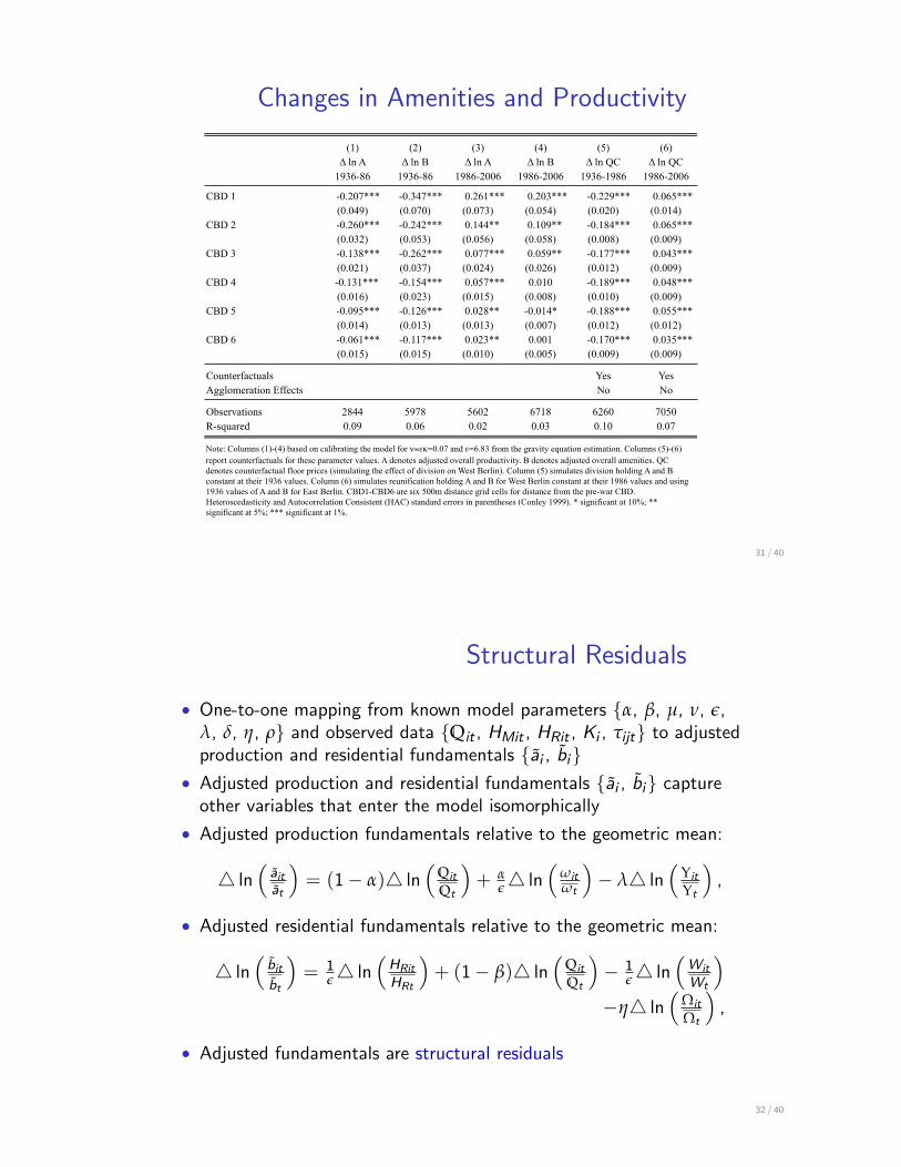
Commuting Data and Model Predictions

-10

12

Resid

ual L

og C

omm

utin

g Pr

obab

ilitie

s

-30 -20 -10 0 10 20Residual Minutes Travel Time

Observations Linear FitNote: Residuals from conditioning on workplace and residence fixed effects.

Panel A: Fit of Gravity Specification 2008

-7-6

-5-4

-3Lo

g Co

mm

utin

g Pr

obab

ility

in M

odel

-7 -6 -5 -4 -3Log Commuting Probability in Micro Data

Observations 45 Degree Line

Panel B: Bilateral District Commuting Probabilities 2008

0.2

.4.6

.81

Cum

ulat

ive P

roba

bility

0 20 40 60 80 100Travel time in minutes

Data Model

Panel C: Cumulative Distribution Berlin Reunification

0.2

.4.6

.81

Cum

ulat

ive P

roba

bility

10 20 30 40 50 60 75 90Travel time in minutes

Data Model

Panel D: Cumulative Distribution West Berlin Division

.2.4

.6.8

1Cu

mul

ative

Pro

babi

lity

20 30 45 60 75 90Travel time in minutes

Data Model

Panel E: Cumulative Distribution Berlin Pre-war

30 / 40

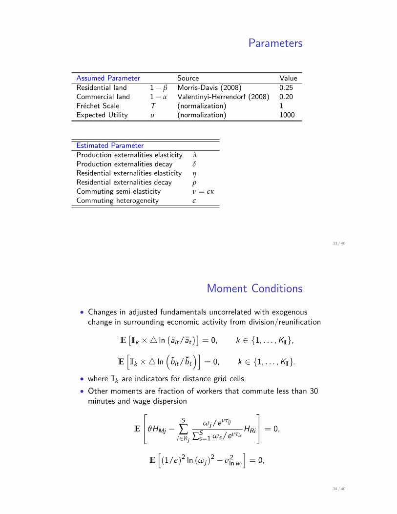
Changes in Amenities and Productivity

(1) (2) (3) (4) (5) (6)Δ ln A Δ ln B Δ ln A Δ ln B Δ ln QC Δ ln QC

1936-86 1936-86 1986-2006 1986-2006 1936-1986 1986-2006

CBD 1 -0.207*** -0.347*** 0.261*** 0.203*** -0.229*** 0.065***(0.049) (0.070) (0.073) (0.054) (0.020) (0.014)

CBD 2 -0.260*** -0.242*** 0.144** 0.109** -0.184*** 0.065***(0.032) (0.053) (0.056) (0.058) (0.008) (0.009)

CBD 3 -0.138*** -0.262*** 0.077*** 0.059** -0.177*** 0.043***(0.021) (0.037) (0.024) (0.026) (0.012) (0.009)

CBD 4 -0.131*** -0.154*** 0.057*** 0.010 -0.189*** 0.048***(0.016) (0.023) (0.015) (0.008) (0.010) (0.009)

CBD 5 -0.095*** -0.126*** 0.028** -0.014* -0.188*** 0.055***(0.014) (0.013) (0.013) (0.007) (0.012) (0.012)

CBD 6 -0.061*** -0.117*** 0.023** 0.001 -0.170*** 0.035***(0.015) (0.015) (0.010) (0.005) (0.009) (0.009)

Counterfactuals Yes YesAgglomeration Effects No No

Observations 2844 5978 5602 6718 6260 7050R-squared 0.09 0.06 0.02 0.03 0.10 0.07

Note: Columns (1)-(4) based on calibrating the model for ν=εκ=0.07 and ε=6.83 from the gravity equation estimation. Columns (5)-(6) report counterfactuals for these parameter values. A denotes adjusted overall productivity. B denotes adjusted overall amenities. QC denotes counterfactual floor prices (simulating the effect of division on West Berlin). Column (5) simulates division holding A and B constant at their 1936 values. Column (6) simulates reunification holding A and B for West Berlin constant at their 1986 values and using 1936 values of A and B for East Berlin. CBD1-CBD6 are six 500m distance grid cells for distance from the pre-war CBD. Heteroscedasticity and Autocorrelation Consistent (HAC) standard errors in parentheses (Conley 1999). * significant at 10%; ** significant at 5%; *** significant at 1%.

31 / 40

Structural Residuals

• One-to-one mapping from known model parameters {a, b, µ, n, e,l, d, h, r} and observed data {Qit , HMit , HRit , Ki , tijt} to adjustedproduction and residential fundamentals {ai , bi}

• Adjusted production and residential fundamentals {ai , bi} captureother variables that enter the model isomorphically

• Adjusted production fundamentals relative to the geometric mean:

4 ln⇣ait

at

⌘= (1� a)4 ln

⇣Qit

Qt

⌘+ a

e4 ln⇣

wit

wt

⌘� l4 ln

⇣Uit

Ut

⌘,

• Adjusted residential fundamentals relative to the geometric mean:

4 ln⇣bit

bt

⌘= 1

e4 ln⇣HRit

HRt

⌘+ (1� b)4 ln

⇣Qit

Qt

⌘� 1

e4 ln⇣Wit

Wt

⌘

�h4 ln⇣

Wit

Wt

⌘,

• Adjusted fundamentals are structural residuals

32 / 40

Parameters

Assumed Parameter Source Value

Residential land 1� b Morris-Davis (2008) 0.25

Commercial land 1� a Valentinyi-Herrendorf (2008) 0.20

Frechet Scale T (normalization) 1

Expected Utility u (normalization) 1000

Estimated Parameter

Production externalities elasticity lProduction externalities decay dResidential externalities elasticity hResidential externalities decay rCommuting semi-elasticity n = ekCommuting heterogeneity e

33 / 40

Moment Conditions

• Changes in adjusted fundamentals uncorrelated with exogenouschange in surrounding economic activity from division/reunification

E⇥Ik ⇥4 ln

�ait/at

�⇤= 0, k 2 {1, . . . ,KI},

EhIk ⇥4 ln

⇣bit/bt

⌘i= 0, k 2 {1, . . . ,KI}.

• where Ik are indicators for distance grid cells

• Other moments are fraction of workers that commute less than 30minutes and wage dispersion

E

2

4JHMj �S

Âi2@j

wj/entij

ÂS

s=1 ws/entisHRi

3

5 = 0,

Eh(1/e)2 ln (wj )

2 � s2lnwi

i= 0,

34 / 40

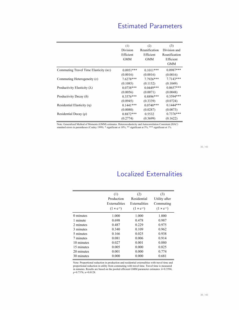
Estimated Parameters

(1) (2) (3)Division Efficient

GMM

Reunification Efficient

GMM

Division and Reunification

Efficient GMM

Commuting Travel Time Elasticity (κε) 0.0951*** 0.1011*** 0.0987***(0.0016) (0.0016) (0.0016)

Commuting Heterogeneity (ε) 7.6278*** 7.7926*** 7.7143***(0.1085) (0.1152) (0.1049)

Productivity Elasticity (λ) 0.0738*** 0.0449*** 0.0657***(0.0056) (0.0071) (0.0048)

Productivity Decay (δ) 0.3576*** 0.8896*** 0.3594***(0.0945) (0.3339) (0.0724)

Residential Elasticity (η) 0.1441*** 0.0740*** 0.1444***(0.0080) (0.0287) (0.0073)

Residential Decay (ρ) 0.8872*** 0.5532 0.7376***(0.2774) (0.3699) (0.1622)

Note: Generalized Method of Moments (GMM) estimates. Heteroscedasticity and Autocorrelation Consistent (HAC) standard errors in parentheses (Conley 1999). * significant at 10%; ** significant at 5%; *** significant at 1%.

35 / 40

Localized Externalities

(1) (2) (3)Production

Externalities (1 × e−δτ)

Residential Externalities

(1 × e−ρτ)

Utility after Commuting

(1 × e−κτ)

0 minutes 1.000 1.000 1.0001 minute 0.698 0.478 0.9872 minutes 0.487 0.229 0.9753 minutes 0.340 0.109 0.9625 minutes 0.166 0.025 0.9387 minutes 0.081 0.006 0.91410 minutes 0.027 0.001 0.88015 minutes 0.005 0.000 0.82520 minutes 0.001 0.000 0.77430 minutes 0.000 0.000 0.681

Note: Proportional reduction in production and residential externalities with travel time and proportional reduction in utility from commuting with travel time. Travel time is measured in minutes. Results are based on the pooled efficient GMM parameter estimates: δ=0.3594, ρ=0.7376, κ=0.0128.

36 / 40

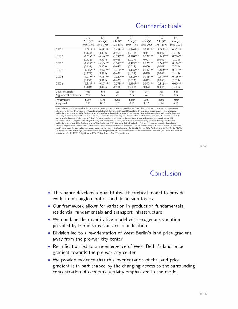
Counterfactuals

(1) (2) (3) (4) (5) (6) (7)Δ ln QC Δ ln QC Δ ln QC Δ ln QC Δ ln QC Δ ln QC Δ ln QC

1936-1986 1936-1986 1936-1986 1936-1986 1986-2006 1986-2006 1986-2006

CBD 1 -0.781*** -0.612*** -0.433*** -0.766*** 0.345*** 1.097*** 0.375***(0.050) (0.030) (0.058) (0.048) (0.041) (0.047) (0.042)

CBD 2 -0.516*** -0.396*** -0.335*** -0.580*** 0.222*** 0.745*** 0.226***(0.032) (0.024) (0.018) (0.027) (0.027) (0.042) (0.026)

CBD 3 -0.414*** -0.306*** -0.308*** -0.489*** 0.153*** 0.568*** 0.174***(0.036) (0.029) (0.030) (0.034) (0.029) (0.041) (0.029)

CBD 4 -0.386*** -0.273*** -0.312*** -0.476*** 0.127*** 0.422*** 0.131***(0.025) (0.018) (0.022) (0.029) (0.019) (0.042) (0.019)

CBD 5 -0.379*** -0.251*** -0.320*** -0.472*** 0.161*** 0.375*** 0.166***(0.030) (0.022) (0.026) (0.037) (0.029) (0.038) (0.029)

CBD 6 -0.314*** -0.207*** -0.275*** -0.394*** 0.090*** 0.312*** 0.094***(0.023) (0.015) (0.021) (0.028) (0.022) (0.034) (0.021)

Counterfactuals Yes Yes Yes Yes Yes Yes YesAgglomeration Effects Yes Yes Yes Yes Yes Yes Yes

Observations 6260 6260 6260 6260 7050 6260 7050R-squared 0.11 0.15 0.07 0.13 0.12 0.24 0.13

Table 7: Counterfactuals

Note: Columns (1)-(6) are based on the parameter estimates pooling division and reunification from Table 5. Column (7) is based on the parameter estimates for division from Table 5. QC denotes counterfactual floor prices. Column (1) simulates division using our estimates of production and residential externalities and 1936 fundamentals. Column (2) simulates division using our estimates of production externalities and 1936 fundamentals but setting residential externalities to zero. Column (3) simulates division using our estimates of residential externalities and 1936 fundamentals but setting production externalities to zero. Column (4) simulates division using our estimates of production and residential externalities and 1936 fundamentals but halving their rates of spatial decay with travel time. Column (5) simulates reunification using our estimates of production and residential externalities, 1986 fundamentals for West Berlin, and 2006 fundamentals for East Berlin. Column (6) simulates reunification using our estimates of production and residential externalities, 1986 fundamentals for West Berlin and 1936 fundamentals for East Berlin. Column (7) simulates reunification using division rather than pooled parameter estimates, 1986 fundamentals for West Berlin, and 2006 fundamentals for East Berlin. CBD1-CBD6 are six 500m distance grid cells for distance from the pre-war CBD. Heteroscedasticity and Autocorrelation Consistent (HAC) standard errors in parentheses (Conley 1999). * significant at 10%; ** significant at 5%; *** significant at 1%.

37 / 40

Conclusion

• This paper develops a quantitative theoretical model to provideevidence on agglomeration and dispersion forces

• Our framework allows for variation in production fundamentals,residential fundamentals and transport infrastructure

• We combine the quantitative model with exogenous variationprovided by Berlin’s division and reunification

• Division led to a re-orientation of West Berlin’s land price gradientaway from the pre-war city center

• Reunification led to a re-emergence of West Berlin’s land pricegradient towards the pre-war city center

• We provide evidence that this re-orientation of the land pricegradient is in part shaped by the changing access to the surroundingconcentration of economic activity emphasized in the model

38 / 40

Thank You

39 / 40

Division and Pre-War CBD

40 / 40