The Economics of Ecosystems and Biodiversity The ...evolution.binghamton.edu/evos/wp-content/uploads/2010/01/Gowdy... · The Economics of Ecosystems and Biodiversity The Ecological

The Economics of Ecosystems and Biodiversity The Ecological and Economic Foundations

(TEEB D0)

Chapter 6

Discounting, ethics and options for maintaining biodiversity and ecosystem integrity

Coordinating Lead Author:

John Gowdy

Lead Authors:

Richard B. Howarth, Clem Tisdell

Reviewers:

Paulus Arnoldus, Bernd Hansjürgens, Cameron Hepburn, Jeffrey McNeely

Review Editor:

Karl-Göran Mäler

September 2009

The Economics of Ecosystems and Biodiversity: The Ecological and Economic Foundations (TEEB D0)

2

Contents

Key messages and recommendations................................................................................................... 3

1 Introduction ..................................................................................................................................... 3

2 The Ramsey discounting equation and intergenerational welfare .............................................. 7

3 Recent behavioral literature on discounting, risk and uncertainty .......................................... 11

4 Ecosystems and biodiversity in the very long run ...................................................................... 14

5 The total value of ecosystems and biodiversity and the discounting equation......................... 16 5.1 The economic value of ecosystems and biodiversity...........................................................16 5.2 The socio-cultural value of ecosystems and biodiversity ....................................................16 5.3 The ecological value of biodiversity to ecosystems.............................................................17

6 Does a low discount rate promote conservation?........................................................................ 17

7 Discounting and safe minimum standards .................................................................................. 20

8 Summary of the major challenges to discounting biodiversity and ecosystem losses.............. 22

References ............................................................................................................................................ 23

Endnotes............................................................................................................................................... 31

Chapter 6: Discounting, ethics and options for maintaining biodiversity and ecosystem integrity

3

Key messages and recommendations

• There are no purely economic guidelines for choosing a discount rate. Responsibility to future

generations is a matter of ethics, best guesses about the well-being of those in future, and preserving life opportunities.

• In general, a higher discount rate will lead to the long-term degradation of biodiversity and

ecosystems. A 5% discount rate implies that biodiversity loss 50 years from now will be valued at only 1/7 of the same amount of biodiversity loss today.

• In terms of the discounting equation, estimates of how well-off those in the future will be is the

key factor as to how much we should leave the future. Should we use income or subjective well-being, or some guess about basic needs?

• A critical factor in discounting is the importance of environmental draw-down (destruction of

natural capital) to estimates of g (as GDP growth). Are we living on savings that should be passed to our descendents?

• A variety of discount rates, including zero and negative rates, should be used depending on the

time period involved, the degree of uncertainty, and the scope of project or policy being evaluated. • A low discount rate for the entire economy might favor more investment and growth and more

environmental destruction.

1 Introduction A central issue in the economic analysis of biodiversity and ecosystems is the characterization of the responsibility of the present generation to those who will live in the future. That is, how will our current use of biological resources affect our future life opportunities and those of our descendents? A common approach is to begin with the Brundtland Commission’s definition of sustainable development, which emphasizes “meeting present needs without compromising the ability of future generations to meet their own needs” (WCED 1987). This definition is very general and has widely different interpretations. In economics, sustainability is often interpreted in terms of maintaining human well-being over intergenerational time scales, though some economists attach special importance to conserving stocks of biodiversity, ecosystem services and other forms of natural capital (see Neumayer 2003). As discussed in the TEEB interim report (TEEB 2008) discounting is key issue in the economics of biodiversity and ecosystems. How should we account for the future effects of biodiversity and ecosystem losses using a variety of valuation methods. This leaves open the question of how to integrate traditional cost-benefit analysis with other approaches to understanding and/or measuring environmental values.


4

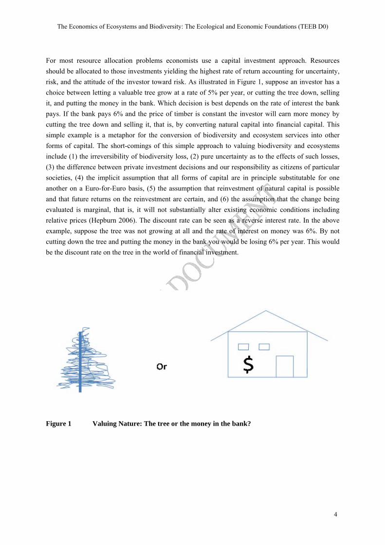
For most resource allocation problems economists use a capital investment approach. Resources should be allocated to those investments yielding the highest rate of return accounting for uncertainty, risk, and the attitude of the investor toward risk. As illustrated in Figure 1, suppose an investor has a choice between letting a valuable tree grow at a rate of 5% per year, or cutting the tree down, selling it, and putting the money in the bank. Which decision is best depends on the rate of interest the bank pays. If the bank pays 6% and the price of timber is constant the investor will earn more money by cutting the tree down and selling it, that is, by converting natural capital into financial capital. This simple example is a metaphor for the conversion of biodiversity and ecosystem services into other forms of capital. The short-comings of this simple approach to valuing biodiversity and ecosystems include (1) the irreversibility of biodiversity loss, (2) pure uncertainty as to the effects of such losses, (3) the difference between private investment decisions and our responsibility as citizens of particular societies, (4) the implicit assumption that all forms of capital are in principle substitutable for one another on a Euro-for-Euro basis, (5) the assumption that reinvestment of natural capital is possible and that future returns on the reinvestment are certain, and (6) the assumption that the change being evaluated is marginal, that is, it will not substantially alter existing economic conditions including relative prices (Hepburn 2006). The discount rate can be seen as a reverse interest rate. In the above example, suppose the tree was not growing at all and the rate of interest on money was 6%. By not cutting down the tree and putting the money in the bank you would be losing 6% per year. This would be the discount rate on the tree in the world of financial investment.

Figure 1 Valuing Nature: The tree or the money in the bank?


5

Box 1: Discounting the Amazon The discussion of the value of the Amazon rainforest illuminates the distinction between economic, cultural, and ecosystem values. The services of the Amazon generate large direct market values, including revenue from ecotourism, fishing, rainforest crops, and pharmaceuticals. Indirect economic benefits include climate regulation, option values for undiscovered rainforest products, and climate change protection form carbon storage. Cultural values not only include the spiritual and life-giving values the Amazon holds for its indigenous people, but also its existence value to the rest of the world’s population. Most of us who know something of the unique and beautiful features of Amazon ecosystems feel a loss when we hear of their destruction even if we have never seen them. But the most important values of the Amazon, as discussed in chapter 1 may be its role in regulating weather in the Western Hemisphere and as the world’s largest storehouse of biodiversity. What role should discounting play in each of these layers of value? As the discussion in chapter 1 shows, when calculating the costs and benefits of a development project, such as a dam, discounting will tend to favor short-term economic benefits such as temporary job creation over the costs of losing environmental services that have smaller annual values but that last indefinitely. Cultural and ecosystems values are difficult or impossible to price and thus are usually excluded by traditional cost benefit analysis. Referring to Figure 1 the services of the Amazon might be represented by the tree. If a section of the Amazon rainforest yields sustainable services equivalent to an annual rate of return of 5% and if the forest could be cut down, sold as timber and invested at a rate of return of 6%, then the economically rational thing to do is to cut down the forest, sell it, and put the money in the bank. But this assumes that investments are secure and last indefinitely and that environmental features and economic investments are completely fungible.

The financial model of resource use is enshrined in the theory of optimal economic growth as described in macroeconomics textbooks (see Blanchard and Fischer 1989, Dasgupta and Heal 1974). This model assumes that society can and should seek to maximize the weighted sum of present and future economic welfare. The weight attached to future welfare declines at ρ percent per year, reflecting society’s impatience, or preference to receive benefits in the short run while deferring costs to the future. In a continuous-time setting with constant population and a single consumption good, this approach employs constrained optimization methods to maximize the social welfare functional:

∫∞

−

0

)]([ dtetCU tρ (1)

subject to the technological, economic, and environmental constraints that force decision-makers to balance short-run and long-run welfare. In this setting, U is instantaneous utility and C is the flow of consumption goods.i This characterization of intertemporal choice, particularly in the cases of biodiversity loss and climate change, has been questioned on both theoretical and behavioral grounds (Bromley 1998, DeCanio 2003, Gowdy 2004, Spash 2002). The model abstracts away from the fact that individuals have finite lifespans and assumes that ρ represents both individuals’ time preference and social preferences regarding tradeoffs between the welfare of present and future generations


6

(Burton 1993, Howarth and Norgaard 1992). Although it is restrictive, the discounted utility framework is mathematically tractable. It is perhaps this fact that explains the model’s widespread use in applied economics. Most importantly, the framework is useful for illuminating the economic, ethical, and cultural aspects of valuing the future impacts of public policies. Beckerman and Hepburn (2007) argue that the practice of utility discounting is justified by the theory of “agent relative ethics.” In this perspective, people reasonably attach greater weight to the welfare of themselves and their immediate family than to people who are less proximate to them in space and time. An early contribution by Dasgupta and Heal (1974), however, showed that the discounted utility criterion sometimes generates outcomes that are unsustainable, yielding a moral paradox that has generated a quite substantial literature. This problem arises in economies that depend on an essential, nonrenewable resource. In this context, short-run economic growth leads to resource depletion that, in turn, leads to long-run economic decline. This occurs because decision-makers are too impatient to make the investments in substitute technologies needed to offset the costs of resource depletion. To address this problem, Solow (1974) proposed the so-called “maximum” social welfare function, which allocates resources in a way that achieves a constant level of utility over time. Conversely, equation (1) may be maximized subject to the constraint that utility is constant or increasing over time (Asheim 1988). In this approach, the utility discount rate represents society’s altruistic preferences towards future generations, or willingness to undertake voluntary sacrifices so that future generations may enjoy a better way of life. The non-declining utility constraint, in contrast, is based on a perceived moral duty to ensure that present actions do not jeopardize the life opportunities available to posterity (Howarth 1995). This approach can be viewed as rational given a rights-based (or “Kantian”) ethical framework in which moral duties complement preference satisfaction in making rational decisions. In applied studies, the discounted utility criterion is often embraced as a sufficient basis for optimal resource allocation, a fact that puts special emphasis on the choice of the utility discount rate. The release of the Stern Review (Stern 2007) and the ensuing debate among economists as to its merit did much to illuminate the role of discounting the costs and benefits of policies having very long time spans and very broad spatial scales—climate change and biodiversity loss being the prime examples. At first the Stern debate centered primarily on the “proper” discount rate to apply to future costs and benefits of climate change mitigation (Ackerman 2008, Dasgupta 2006, Mendelson 2006-7, Yohe and Tol 2007). As the debate progressed it became clear that there was more to the economics of climate change than choosing the “correct” discount rate. Several prominent environmental economists came to the conclusion that the standard economic model offers an inadequate framework to analyze environmental issues characterized by irreversibility’s, pure uncertainty, and very long time horizons (Dasgupta 2008, Weitzman 2009). The “key messages” in the Stern Review’s economic analysis of climate change (chapter 2, p. 25) apply with equal force to the economic analysis of biodiversity. Biodiversity and ecosystem loss has properties that make it difficult to apply standard welfare analysis including discounting the future:


7

1. It is a global phenomenon with global consequences. 2. Its impacts are long-term and irreversible. 3. Pure (or “Knightian”) uncertainty is pervasive. 4. Changes are non-marginal and non-linear. 5. Questions of inter- and intra-generational equity are central.

These points have been made forcefully for decades by economists working outside the neoclassical paradigm (Boulding 1973, Daly 1977, Georgescu-Roegen 1971). Interestingly, it seems that the policy prescriptions of both those using a more conventional welfare economics approach, and those who call for an alternative, heterodox approach to environmental valuation, are converging. Using either standard or alternative approaches, when the services of nature are taken into account, sustaining human welfare in the future implies aggressive conservation and ecosystem restoration policies in the present. This chapter is organized as follows. Section 2 discuss the economic approach to intergenerational welfare using the Ramsey discounting equation, section 3 reviews some recent findings from behavioral economics and their relevance to the discounting issue, section 4 examines the issue of ecosystems an biodiversity preservation in the very long run, section 5 discusses the discounting equation in the context of the total value of ecosystems and biodiversity, section 6 examines the macroeconomic implications on biodiversity of a low discount rate, section 7 looks at the issue of discounting and the safe minimum standard, and ecosystem services and the poor, section 8 concludes.

2 The Ramsey discounting equation and intergenerational welfare

In optimal growth theory, it is common to assume that the utility function presented in equation (1)

takes the specific form )1/()( 1 ηη −= −CCU . Here η is a parameter that reflects the curvature of the

utility function. Given this assumption, future monetary costs and benefits should be discounted at the rate r that is defined by the so-called “Ramsey equation”: r = ρ + η • g (2) The discount rate r is determined by the rate of pure time preference (ρ), η, and the rate of growth of per capita consumption (g). In intuitive terms, people discount future economic benefits because: (a) they are impatient; and (b) they expect their income and consumption levels to rise so that 1 Euro of future consumption will provide less satisfaction than 1 Euro of consumption today. This equation abstracts away from uncertainty, a fact that streamlines the analysis but that reduces the model’s plausibility and descriptive power. Accounting for uncertainty leads to a more complex specification in which the discount rate equation includes a third term that reflects the perceived risk of the action under consideration (see Blanchard and Fischer 1989, chapter 6 and Starrett 1988). As noted above, the rate of pure time preference (ρ) is supposed to reflect both individuals’ time preferences and social preferences regarding the value of the well-being of future generations as seen


8

from the perspective of those living today. More realistic models distinguish between these effects, and blending them together can obscure important aspects of both descriptive modeling and prescriptive analysis (Gerlagh and Keyzer 2001, Howarth 1998, Auerbach and Kotlikoff 1987). A positive value for ρ means that, all other things being equal, the further into the future we go the less the well-being of persons living there is worth to us. The higher the value of ρ the less concerned we are about negative impacts in the future. A large literature exists arguing for a variety of values for pure time preference but it is clear by now that there is no econometric method to determine the value of ρ. Choosing the rate of pure time preference comes down to a question of ethics. Ramsey (1928, 261) asserted that a positive rate of pure time preference was “ethically indefensible and arises merely from a weakness of the imagination.” On the other side of the debate, Pearce et al. (2003) took the position that a positive time preference discount rate is an observed fact since people do in fact discount the value of things expected to be received in the future. Nordhaus (1992, 2007) has consistently argued that the market rate of interest constitutes the appropriate discount rate that reveals individuals’ time preference.ii Sen’s (1961) “isolation paradox” casts doubt on the argument that the social discount rate should be set equal to the market rate of return. According to Sen, private investments may provide spillover benefits that are not captured by individual investors. Providing bequests to one’s daughter, for example, serves to increase the welfare of the daughter’s spouse and, by extension, his parents. When preferences are interconnected in this way, individuals underinvest. Correcting this market failure would lead to increased investment, lower interest rates, and therefore a lower discount rate in cost-benefit analysis (Howarth and Norgaard 1993).But even if we agree to use a market rate, which market rate should be used? In the United States, a voluminous literature has focused on the fact that, since the late 1920s, safe financial instruments such as bank deposits and short-run government bonds yield average returns of roughly 1%. Corporate stocks, in contrast, yielded average returns of 7% per year with substantial year-to-year volatility. Assets with intermediate risks (such as corporate bonds and long-term government bonds that carry inflation risks) pay intermediate returns. (See Cochrane 2001, for an authoritative textbook discussion). Choosing a discount rate, then, involves a judgment regarding the perceived riskiness of a given public policy (Starrett 1988). Low discount rates are appropriate for actions that yield safe benefit streams or provide precautionary benefits – i.e., that reduce major threats to future economic welfare.iii Biodiversity loss and climate change will affect the entire world’s population including those from cultures with very different ideas about obligations to the future. Furthermore, Portney and Weyant (1999, p. 4) point out that “[t]hose looking for guidance on the choice of discount rate could find justification [in the literature] for a rate at or near zero, as high as 20 percent, and any and all values in between” (quoted in Cole 2008). Frederick et al. (2004) report empirical estimates of discount rates ranging from -6% to 96,000%. Others argue that discounting from the perspective of an individual at a point in time is not equivalent to a social discount rate reflecting the long term interest of the entire human species. An observed positive market discount rate merely shows that market goods received in the future are worth less as evaluated by an individual living now, not that they are worth less at the point in the future that they are received.


9

The other important factor in the Ramsey equation determining how much we should care about the future is how well-off those in the future are likely to be. As shown in equation (2), the standard model characterizes the well-being of future generations using two components, the growth rate of per capita income in the future (g) and the elasticity of the marginal utility of consumption (η). The elasticity of marginal utility measures how rapidly the marginal utility of consumption falls as the consumption level increases. It is often assumed that η is equal to 1 (Nordhaus 1994, Stern 2007). In this case, then ηg corresponds to a Bernoulli (logarithmic) utility function, and 1% of today’s income has the same value as 1% of income at some point in the future (since g is a percentage change). So if per capita income today is $10,000 and income in the year 2100 is $100,000, $1,000 today has the same value as $10,000 in 2100. Put another way, a $1,000 sacrifice today would be justified only if it added at least $10,000 to the average income of people living in the year 2100 (Quiggin 2008). The higher the value of η, the higher the future payoff must be for a sacrifice today. For example, with ρ near zero and a positive value for g, increasing η from 1 to 2 would double the discount rate. A number of assumptions are buried in the parameter η as it is usually formulated. It is assumed that η is independent of the level of consumption, that it is independent of the growth rate of consumption, and that social well-being can be characterized by per capita consumption. These assumptions are arbitrary and adopted mainly for convenience (Pearce et al. 2006). At least three distinct valuation concepts are present in η (Cole 2008, 18). It contains a measure of risk aversion, a moral judgment about static income inequality among present day individuals, and a moral judgment about dynamic income inequality over time. Weitzman (2009) notes that the values of these components move the discount rate in different directions. On one hand a high value for η (in conjunction with g) would seem to take the moral high ground—a given loss in income has a greater negative impact on a poor person than a rich person. But if we assume, as most economic models do, that per capita consumption g continues to grow in the future, a higher η means a higher value for ηg and the less value we place on income losses for those in the future. Assuming a near-zero value for ρ and that η = 1 (as in Cline 1992 and Stern 2007) means that the total discount rate (r) is determined by projections of the future growth rate of per capita income, g. The growth rate of income is derived from projecting past world economic performance and the researcher’s judgment. The values of g in the Stern report and in the most widely used climate change models range between 1.5% and 2.0% (Quiggin 2008, 12). With a high g, discounting the future is justified by the assumption that those living in the future will be better off than those living today (Pearce et al. 2006). In the TEEB interim report (TEEB 2008, p. 30) Martinez-Alier argues that assuming constant growth in g leads to the “optimist’s paradox.” The assumption of continual growth justifies the present use of more resources and more pollution because our descendents will be better off. But such growth would leave future generations with a degraded environment and a lower quality of life. A major step forward in understanding the economics of sustainability was the realization that maintaining a constant or increasing level of consumption or utility depends on maintaining the stock


10

of capital assets generating that welfare (Arrow et al. 2004, Dasgupta and Mäler 2000, Hartwick 1977, 1997, Solow 1974). Thus, maintaining a non-declining g means maintaining (1) productive manufactured physical capital, (2) human capital—knowledge, technical know-how, routines, habits and customs—and the institutions supporting it, and (3) natural capital. Using the terminology in chapter 1, the biodiversity component of natural capital is, in turn, comprised of three different kinds of value to humans:

1. Economic – The direct inputs from nature to the market economy, 2. Socio-cultural – The non-market services necessary for maintaining the biological and

psychological needs of the human species, and

3. Ecological value – The value to ecosystems such as preserving evolutionary potential through biological diversity and ecosystem integrity.

These layers of biodiversity value are discussed in more detail in section 5. Under certain technical assumptions, g may be interpreted as the growth rate of per capita income adjusted for externalities and other market imperfections. Under these conditions, Dasgupta and Mäler (2000) show that g can be considered as the rate of return on all forms of capital. In a dynamic growth context, g is equivalent to the growth rate of total factor productivity (TPF) along a balanced growth path. TFP is the rate of growth of economic output not accounted for by the weighted growth rates of productive inputs. In the three input case used here, • • • • TFP = Q – aMK – bHK – cNK , a+b+c = 1 and the weights are input cost shares (3) For example, in a simple model using manufactured capital (MK), human capital (HK), and natural capital (NK) as inputs, if output grows by 5% per year and the weighted average growth rates of inputs increases by 4%, then TFP would be 1%. Environmental economists have long maintained that estimates of TFP (g in the Ramsey model) do not adequately take into account the draw-down of the stock of natural capital (Ayres and Warr 2006, Dasgupta and Mäler 2000, Repetto et al. 1989). Vouvaki and Xeapapadeas (2008) found that when the environment is not considered as a factor of production TFP estimates are biased upward. They argue that failing to internalize the cost of an environmental externality is equivalent to using an unpaid factor of production. After including as natural capital only the external effects of CO2 pollution from energy use, they found that TFP estimates for 19 of 23 countries switched from positive to negative. The average of TFP estimates for the 23 countries changed from +0.865 to -0.952. This result implies that when the negative effects of economic production on the ability of natural world to provide productive inputs g could well be negative—future generations will be worse off. Moreover, when environmental degradation effects beyond CO2 accumulation are included the case for a negative g becomes even stronger. This has serious implications for long run economic policies for climate change mitigation and biodiversity


11

loss. Given some reasonable assumptions about pure time preference and the elasticity of consumption, a negative g implies that the present generation should consume less in order to invest more in the well-being of future generations. If we step back from the assumption that the well-being of future generations can be characterized by per capita consumption—by, for example, considering g as representing subjective well-being (Kahneman et al. 1997)—the case for considering a negative g becomes even stronger. Among the most important findings of the subjective well-being literature are these: (1) traditional economic indicators such as per capita NNP are inadequate measures of welfare, (2) the effect of an income change depends on interpersonal comparisons and relative position, (3) humans have common, identifiable biological and psychological characteristics related to their well-being (Frey and Stutzer 2002, Layard 2005). These observations have direct bearing on the sustainability debate and have the potential to guide intergenerational welfare and policies to protect biological diversity. People receive economic benefits from biodiversity but there are also psychological and aesthetic benefits that cannot be properly captured by market values (Wilson 1994). All these contributions of biodiversity are being rapidly reduced and should be taken into account in estimates of future well-being (g). Dasgupta (1995) argues further that there are self-reinforcing links between environmental degradation including biodiversity loss, poverty, and population growth.

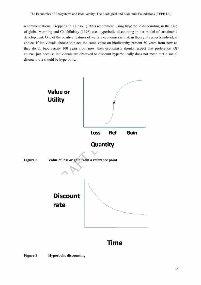
3 Recent behavioral literature on discounting, risk and uncertainty Insights from behavioral economics have greatly broadened our understanding of how people compare future costs and benefits. Relevant insights into human behavior include the following: 1. Loss Aversion – Losses are given higher values than equivalent gains. As illustrated in Figure 2 (from Knetsch 2005) there is considerable evidence that people are loss averse, that is, they evaluate gains and losses from a reference point and place a higher value a loss than on a gain of an equal amount of that same thing (Kahneman and Tversky 1979). This is confirmed in the widely reported discrepancy between willingness to pay (WTP) and willingness to accept (WTA) measures of environmental changes (Brown and Gregory 1999). The implications for evaluating biodiversity loss are clear. Even in the context of standard utility theory, the required compensation for biodiversity loss (WTA) is likely to be much greater than the estimated market value of that loss (WTP).

2. Hyperbolic Discounting – There is some evidence that people discount the future hyperbolically, that is, as shown in Figure 3, the discount rate declines then flattens out so that after some time the present value of something does not significantly decline (Laibson 1997). The existence of hyperbolic discounting implies that standard economic analysis may seriously underestimate the long-term benefits of biodiversity protection. If people discount hyperbolically, and if we respect stated preferences, straight-line discounting should not be used to place values on distant-future environmental damages such as those caused by biodiversity loss. Hyperbolic discounting has been widely discussed in the theoretical literature and has had some impact on policy


12

recommendations. Cropper and Laibson (1999) recommend using hyperbolic discounting in the case of global warming and Chichilnisky (1996) uses hyperbolic discounting in her model of sustainable development. One of the positive features of welfare economics is that, in theory, it respects individual choice. If individuals choose to place the same value on biodiversity present 50 years from now as they do on biodiversity 100 years from now, then economists should respect that preference. Of course, just because individuals are observed to discount hyperbolically does not mean that a social discount rate should be hyperbolic.

Figure 2 Value of loss or gain from a reference point

Figure 3 Hyperbolic discounting


13

Beltratti et al. (1998) advocate the use of the “green golden rule” for renewable resource, using something near market discount rates in the short run (so that the present is not exploited) and a rate asymptotically approaching zero in the long run (so that the distant future is not exploited). Similarly, Weitzman (2001) advocates what he terms “gamma discounting” using a rate of about 4 percent for the immediate future with a steady decline to near zero in the distant future. 3. Inconsistent Discounting – Rubinstein (2003) points out that hyperbolic discounting has been accepted by many economists because it can be easily incorporated into the net present value framework of standard economic analysis. He argues that the evidence suggests that the larger problem is inconsistent, not hyperbolic, discounting. People appear to have different discount rates for different kinds of outcomes (Loewenstein 1987). Considerable evidence exists that people are wildly inconsistent even when discounting similar things. Inconsistent discounting suggests that there may be limits to attempts to placing precise numbers on the general tendency of individuals to prefer something now rather than later. 4. The Equity Premium Puzzle – Mehra and Prescott (1985) showed the discounted utility model is deeply inconsistent with the observed gap between the low returns available on safe investments and the much higher average returns paid provided by risky assets such as corporate stocks. Mankiw and Zeldes (1991) calculate that the level of risk aversion implied by this rate-of-return spread implies that an investor would have to be indifferent between a bet equally likely to pay $50,000 or $100,000 (with an expected value of $75,000) and a certain payoff of $51,209. Explaining the low market return on safe assets requires that both ρ and η must assume values near zero (Kocherlakota 1996). Yet explaining the high risk premium paid by stocks requires that investors must be highly risk averse, which implies that η must attain a high, positive value to be consistent with the data. Scientifically, this suggests that the discounted utility model is in a deep sense inconsistent with empirical observations. This point undercuts reliance on equation (2) to calculate discount rates. A variety of approaches have been advanced to address this disparity (see Kocherlakota 1996, Cochrane 2001). Some models have extended preferences to distinguish between risk preferences and the elasticity of intertemporal substitution. Others assume that preferences are shaped by habit formation and/or relative consumption effects. A third hypothesis is that investors are loss averse with respect to investment gains and losses (Benartzi and Thaler 1995). Including this effect in the utility function serves to decouple the social discount rate from the market rate of return (Howarth 2009). In this case, the public policies should be discounted at a rate that is close to the risk-free rate of return, even for policies that involve significant degrees of uncertainty. 5. Discounting under Uncertainty – On theoretical grounds, there is reason to believe that greater uncertainty about the future tends to produce lower certainty-equivalent discount rates (Gollier 2008). This is because investing in safe assets reduces the risks pertaining to future economic welfare, rendering them attractive to investors even at low rates of return. Newell and Pizer (2003) used random walk and mean-reverting models to compute certainty equivalent discount rates that measure the uncertainty adjusted rate out into the distant future. When applied to climate change scenarios,


14

their results suggested that the present value of mitigation efforts almost doubled. Hepburn et al. (2009) extended this result to estimate autoregressive and regime-switching models of U.S. interest rates and also found that uncertainty-adjusted rates declined more rapidly. Uncertainty is pervasive in the case of the welfare effects of biodiversity loss and this suggests using lower discount rates in valuing future losses of biodiversity and ecosystem services. 6. Discounting and Relative Prices – The discount rate is applied to an aggregate consumption good and an implicit assumption is that the prices of all goods are changing at the same rate. But biodiversity is not an average consumption good. For at least two reasons—increasing scarcity and limits to its substitutability—the rate of change of the relative price of biodiversity will be different from a typical consumption good (Cameron Hepburn, personal communication). Sterner and Persson (2008, p. 62) write: Briefly, because the rate of growth is uneven across sectors of the economy, the composition of economic output will inevitably change over time. If output of some material goods (e.g. mobile phones) increases, but access to environmental goods and services (e.g. access to clean water, rain-fed agricultural production, or biodiversity) declines, then the relative price of these environmental amenities should rise over time. This would mean that the damages from biodiversity loss (or the benefits from biodiversity preservation) would be augmented and this might be great enough to offset the effect of the positive discount rate. If this is the case, increasing the amount of biodiversity and ecosystems would be economically justified (Hoel and Sterner 2007). 7. Risk Aversion and Insurance – A large body of evidence suggests that people are risk averse (Kahneman and Tversky 1979). This has major implications for evaluating biodiversity and ecosystem losses. As in the case of climate change there is a real, although unknown, possibility that biodiversity loss will have catastrophic effects on human welfare. Paul and Anne Ehrlich (1997) use the “rivet popper” analogy to envision the effects of biodiversity loss. A certain number of rivets can pop out of an airplane body without causing any immediate danger. But once a critical threshold is reached the airplane becomes unstable and crashes. Likewise, ecosystems are able to maintain themselves with a certain range of stress, but after a point they may experience a catastrophic flip from a high biodiversity stable state to another, low diversity stable state. Weitzman (2009) uses the evidence for a small, but significant, possibility of a runaway greenhouse effect to argue for aggressive climate change mitigation policies.

4 Ecosystems and biodiversity in the very long run Many economists (for example Spash 2002, chapters 8 and 9) question the appropriateness of discounting as applied to global and far-reaching issues like biodiversity loss. Ultimately, human existence depends on maintaining the web of life within which we co-evolved with other species and thus the idea of placing a discounted “price” on total biodiversity is absurd. One may object that the


15

ability to adapt to environmental change is one of the most striking characteristics of Homo sapiens (Richerson and Boyd 2005). But the rapidity of current and projected environmental change is unique in our history. Human activity within the past one hundred years or so has drastically altered the course of biological evolution on planet earth. According to a survey by the International Union for the Conservation of Nature, a quarter of mammal species face extinction (Gilbert 2008). Conservative estimates indicate that 12% of birds are threatened, together with 30% of amphibians and 5% of reptiles. Particularly alarming is the state of the world’s oceans. Human-caused threats to ocean biodiversity are summarized by Jackson (2008, p. 11458):

“Today, the synergistic effects of human impacts are laying the groundwork for a comparatively great Anthropocene mass extinction in the oceans with unknown ecological and evolutionary consequences. Synergistic effects of habitat destruction, overfishing, introduced species, warming, acidification, toxins and mass runoff of nutrients are transforming once complex ecosystems like coral reefs into monotonous level bottoms, transforming clear and productive coastal seas into anoxic dead zones, and transforming complex food webs topped by big animals into simplified, microbially dominated ecosystems with boom and bust cycles of toxic dinoflagellate blooms, jellyfish, and disease.”

If we modeled ecosystems according to the Solow-Hartwick approach for economic sustainability (maintaining the capital stock necessary to insure that economic output does not decline) it would certainly be clear that the “ecosystem capital” base for sustaining biodiversity is being rapidly depleted. If the biologists and paleontologists who study the problem are correct, we are entering into the sixth mass extinction of complex life on the planet during the last 570 million years or so. Biodiversity recovery from past mass extinctions took between 5 and 20 million years to recover (Ward 1994, Wilson 1998). Past mass extinctions irreversibly restructured the composition of the earth’s biota (Krug et al. 2009). Even if the final result of the current mass extinction is a richer, more biologically diverse world, as occurred after past mass extinctions, humans will not be around to see it. Human-induced biodiversity loss will constrain the evolution of humans and other species for as long as humans will inhabit planet earth. This prospect raises entirely new kinds of questions about how to value today’s impact on future generations. These include:

1. Functional transparency (Bromley 1989) – In many cases the role of a particular species in an ecosystem is apparent only after it has been removed. The change may be non-linear and irreversible. The effect on local economies may be catastrophic as in the collapse the Northern Cod fishery due to overharvesting. More than 40,000 people in Newfoundland lost their jobs and the cod fishery has still not recovered 15 years after a total moratorium on cod fishing.

2. Preserving genetic and ecosystem diversity (Gowdy 1997) – Evolutionary potential is the

ability of a species or ecosystem to respond to changing conditions in the future. Future conditions are largely unpredictable (the effects of climate change on biodiversity, for example) but in general the greater the diversity of an ecosystem, the more resilient that system is (Tilman and Downing 1994).


16

3. Preserving options for future generations (Page 1983, Norton 2005). The financial model of sustainability treats biodiversity as an input for commodity production. Even if the notion of consumer utility is broadened to include things like existence values, the model’s frame of reference is till the industrial market economy. The effects of present day biodiversity loss and ecosystem disruption will last for millennia. The question becomes what do we leave future generations if we have no idea what sorts of economies/values/needs they will have?

5 The total value of ecosystems and biodiversity and the discounting equation

The total value of ecosystems and biodiversity is unknown but we do know that the ultimate value to humans is infinite because if it is reduced beyond a certain point our species could not exist. Biodiversity value can be seen as layers of a hierarchy moving from market value, to non-market value to humans, to ecosystem value. These various levels of biodiversity value point to the need for a pluralistic and flexible methodology to determine appropriate policies for its use and preservation (Gowdy 1997).

5.1 The economic value of ecosystems and biodiversity

Economic value includes the direct economic contributions of biodiversity including eco-tourism, recreation, and the value of direct biological inputs such as fisheries and forests. These values can be very large. For example, Geist (1994) estimated that the direct economic value of Wyoming’s big game animals, from tourism and hunting, exceeded $1 billion or about $1,000 for every large animal. Although evidence from contingent valuation, hedonic pricing and other economic valuation tools underscore the importance of biodiversity and ecosystems, these give incomplete, lower-bound estimates of their values (see Nunes and van den Bergh 2001). The degree to which an economically valuable biological resource should be exploited is driven by the social discount rate, r in equation (2) above. The rate determines how to split the stock of natural capital between consumption now and consumption in the future.

5.2 The socio-cultural value of ecosystems and biodiversity

The biological world contributes to human psychological well-being in ways that can be empirically measured (Kellert 1996, Wilson 1994). But measures of subjective well-being cannot be adequately valued in a traditional social welfare framework (Norton 2005, Orr 2005). Spiritual, cultural, aesthetic, and other contributions of interacting with nature may be included in a more comprehensive conception of utility such as the Bentham/Kahneman notion of utility as well-being. Discounting non-market values of biodiversity– what should we leave future generations? Is there any reason to think those in the future will not have the same psychological need for interacting with nature? Is there any reason to believe that a walk in a rainforest is worth more to a person living now than to a person living 1, 50, or 100 years from now? The reasonable answer is no. The appropriate


17

discount rate for this part of biodiversity, the pure time preference of biophilia, is ρ = 0. Another interesting interpretation of ρ in this context would be consider it as the discount rate if a person were behind a Rawlsian veil of ignorance not knowing where in time she would be placed (Dasgupta 2008).

5.3 The ecological value of biodiversity to ecosystems

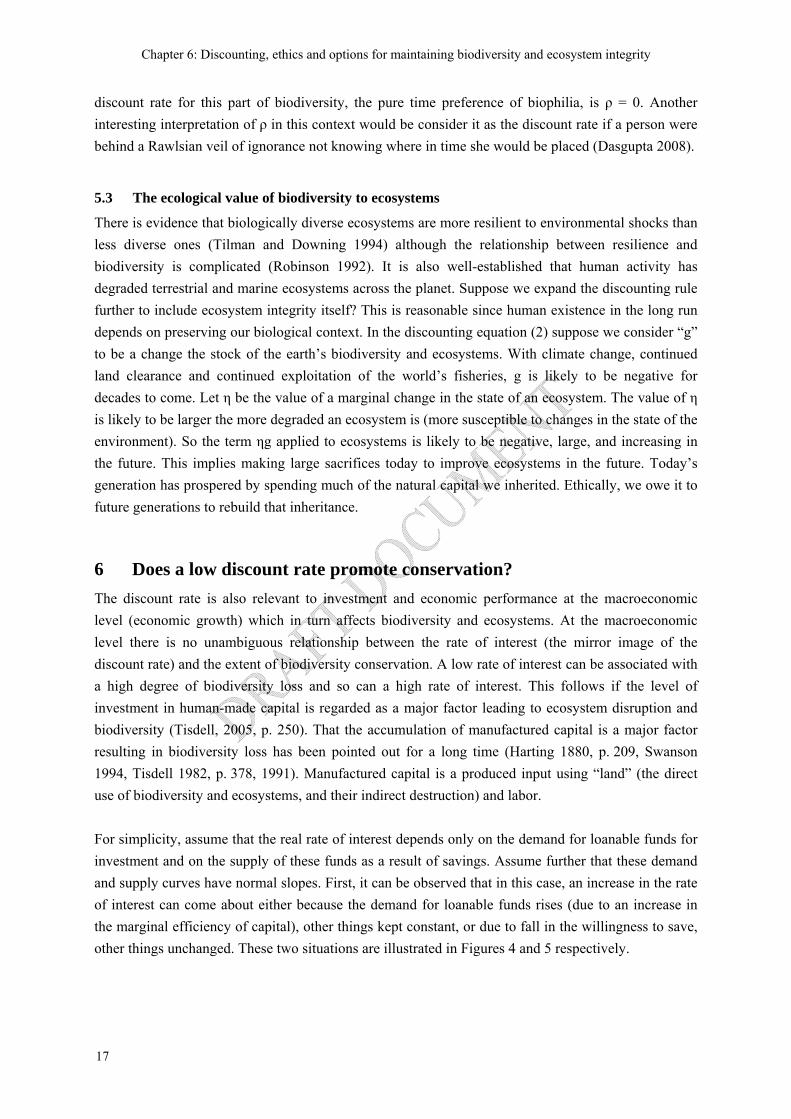
There is evidence that biologically diverse ecosystems are more resilient to environmental shocks than less diverse ones (Tilman and Downing 1994) although the relationship between resilience and biodiversity is complicated (Robinson 1992). It is also well-established that human activity has degraded terrestrial and marine ecosystems across the planet. Suppose we expand the discounting rule further to include ecosystem integrity itself? This is reasonable since human existence in the long run depends on preserving our biological context. In the discounting equation (2) suppose we consider “g” to be a change the stock of the earth’s biodiversity and ecosystems. With climate change, continued land clearance and continued exploitation of the world’s fisheries, g is likely to be negative for decades to come. Let η be the value of a marginal change in the state of an ecosystem. The value of η is likely to be larger the more degraded an ecosystem is (more susceptible to changes in the state of the environment). So the term ηg applied to ecosystems is likely to be negative, large, and increasing in the future. This implies making large sacrifices today to improve ecosystems in the future. Today’s generation has prospered by spending much of the natural capital we inherited. Ethically, we owe it to future generations to rebuild that inheritance.

6 Does a low discount rate promote conservation? The discount rate is also relevant to investment and economic performance at the macroeconomic level (economic growth) which in turn affects biodiversity and ecosystems. At the macroeconomic level there is no unambiguous relationship between the rate of interest (the mirror image of the discount rate) and the extent of biodiversity conservation. A low rate of interest can be associated with a high degree of biodiversity loss and so can a high rate of interest. This follows if the level of investment in human-made capital is regarded as a major factor leading to ecosystem disruption and biodiversity (Tisdell, 2005, p. 250). That the accumulation of manufactured capital is a major factor resulting in biodiversity loss has been pointed out for a long time (Harting 1880, p. 209, Swanson 1994, Tisdell 1982, p. 378, 1991). Manufactured capital is a produced input using “land” (the direct use of biodiversity and ecosystems, and their indirect destruction) and labor. For simplicity, assume that the real rate of interest depends only on the demand for loanable funds for investment and on the supply of these funds as a result of savings. Assume further that these demand and supply curves have normal slopes. First, it can be observed that in this case, an increase in the rate of interest can come about either because the demand for loanable funds rises (due to an increase in the marginal efficiency of capital), other things kept constant, or due to fall in the willingness to save, other things unchanged. These two situations are illustrated in Figures 4 and 5 respectively.


18

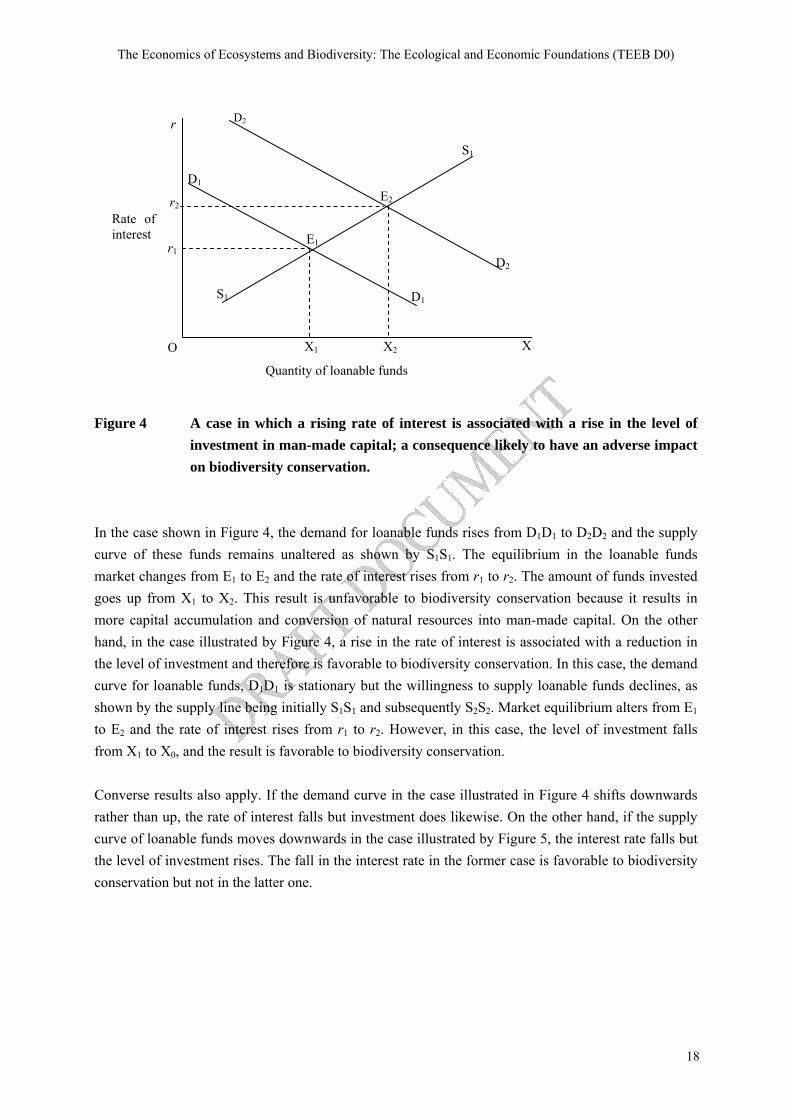
Figure 4 A case in which a rising rate of interest is associated with a rise in the level of

investment in man-made capital; a consequence likely to have an adverse impact on biodiversity conservation.

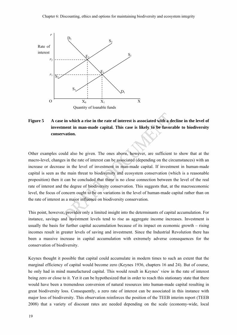
In the case shown in Figure 4, the demand for loanable funds rises from D1D1 to D2D2 and the supply curve of these funds remains unaltered as shown by S1S1. The equilibrium in the loanable funds market changes from E1 to E2 and the rate of interest rises from r1 to r2. The amount of funds invested goes up from X1 to X2. This result is unfavorable to biodiversity conservation because it results in more capital accumulation and conversion of natural resources into man-made capital. On the other hand, in the case illustrated by Figure 4, a rise in the rate of interest is associated with a reduction in the level of investment and therefore is favorable to biodiversity conservation. In this case, the demand curve for loanable funds, D1D1 is stationary but the willingness to supply loanable funds declines, as shown by the supply line being initially S1S1 and subsequently S2S2. Market equilibrium alters from E1 to E2 and the rate of interest rises from r1 to r2. However, in this case, the level of investment falls from X1 to X0, and the result is favorable to biodiversity conservation. Converse results also apply. If the demand curve in the case illustrated in Figure 4 shifts downwards rather than up, the rate of interest falls but investment does likewise. On the other hand, if the supply curve of loanable funds moves downwards in the case illustrated by Figure 5, the interest rate falls but the level of investment rises. The fall in the interest rate in the former case is favorable to biodiversity conservation but not in the latter one.

r

r2

r1

O X1 X2 X

Quantity of loanable funds

D1

D2

S1

E1

E2

D1

D2

S1

Rate of interest


19

Figure 5 A case in which a rise in the rate of interest is associated with a decline in the level of

investment in man-made capital. This case is likely to be favorable to biodiversity conservation.

Other examples could also be given. The ones above, however, are sufficient to show that at the macro-level, changes in the rate of interest can be associated (depending on the circumstances) with an increase or decrease in the level of investment in man-made capital. If investment in human-made capital is seen as the main threat to biodiversity and ecosystem conservation (which is a reasonable proposition) then it can be concluded that there is no close connection between the level of the real rate of interest and the degree of biodiversity conservation. This suggests that, at the macroeconomic level, the focus of concern ought to be on variations in the level of human-made capital rather than on the rate of interest as a major influence on biodiversity conservation. This point, however, provides only a limited insight into the determinants of capital accumulation. For instance, savings and investment levels tend to rise as aggregate income increases. Investment is usually the basis for further capital accumulation because of its impact on economic growth – rising incomes result in greater levels of saving and investment. Since the Industrial Revolution there has been a massive increase in capital accumulation with extremely adverse consequences for the conservation of biodiversity. Keynes thought it possible that capital could accumulate in modern times to such an extent that the marginal efficiency of capital would become zero (Keynes 1936, chapters 16 and 24). But of course, he only had in mind manufactured capital. This would result in Keynes’ view in the rate of interest being zero or close to it. Yet it can be hypothesized that in order to reach this stationary state that there would have been a tremendous conversion of natural resources into human-made capital resulting in great biodiversity loss. Consequently, a zero rate of interest can be associated in this instance with major loss of biodiversity. This observation reinforces the position of the TEEB interim report (TEEB 2008) that a variety of discount rates are needed depending on the scale (economy-wide, local

r

r2

r1

O X0 X1 X

S1

S2

E2

E1

S1

S2 D1

D1

Quantity of loanable funds

Rate of interest


20

community or individual), the timeframe (immediate or distant future), and income group being considered (rich or poor).

7 Discounting and safe minimum standards There is a long tradition in resource economics of applying a higher discount rate to the benefits of development and a lower rate to the environmental costs of that development. Fisher and Krutilla (1985) suggest a formula for estimating the net present value for a development project that reduces to: NPV(D) = -1 + D/(r+k) – P(r-h) (4) Where D is the value of development and P is the value of preservation. In this setup, a factor k is added to the discount rate applied to development benefits to reflect the depreciation of development benefits over time. In a similar vein, a factor h is subtracted from the rate of discount applied to the benefits of preservation. Here h is supposed to represent growth in the value of environmental services over time based on increased material prosperity that augments willingness to pay for scarce nonmarket goods. No hard and fast rules can be applied to determine exactly how much these discount rates should be adjusted. This status quo bias mentioned above lends support to the notion of a safe minimum standard (SMS) and the precautionary principle. The SMS approach (Bishop 1978) explicitly recognizes that irreversible environmental damage should be avoided unless the social costs of doing so are “unacceptably high.” The concept is necessarily vague because it does not rely on a single money metric. It recognizes that a discount premium should be applied to environmental losses, that economic gains should be discounted more heavily, that a great amount of uncertainty is involved in judging the effects of environmental losses, and that there are limits to substituting manufactured goods for environmental resources. Rights based or deontological values are widely held, as indicated by numerous valuation surveys (Lockwood 1998, Spash 1997, Stevens et al. 1991). A rights-based approach may be especially appropriate for policies affecting future generations (Howarth 2007, p. 1983). Do future generations have a right to clean air, clean water, and an interesting and varied environment? There is no reason to think that future generations would be any more willing than we are to have something taken away from them forever (especially things like a stable climate and biological species) as long as they are compensated by something “of equal value.” A rights-based approach to sustainability moves us away from the welfare notions of tradeoffs and fungibility toward the two interrelated concerns of uniqueness and irreversibility. As Bromley (1998, p. 238) writes: “Regard for the future through social bequests shifts the analytical problem to a discussion about deciding what, rather than how much, to leave for those who will follow.” The question of what to leave also moves us away from marginal analysis, and concern only about relative amounts of resources, toward looking at discontinuous changes and the basic biological requirements of the human species in evolutionary context.


21

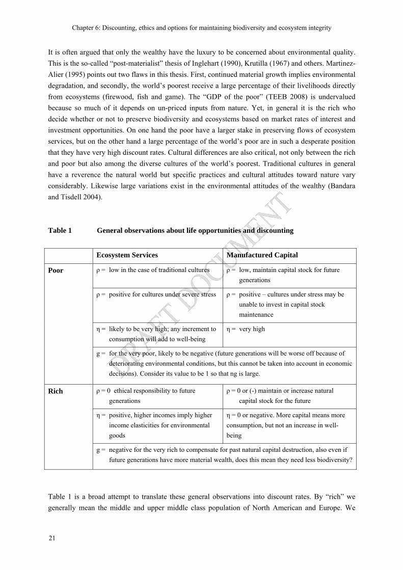
It is often argued that only the wealthy have the luxury to be concerned about environmental quality. This is the so-called “post-materialist” thesis of Inglehart (1990), Krutilla (1967) and others. Martinez-Alier (1995) points out two flaws in this thesis. First, continued material growth implies environmental degradation, and secondly, the world’s poorest receive a large percentage of their livelihoods directly from ecosystems (firewood, fish and game). The “GDP of the poor” (TEEB 2008) is undervalued because so much of it depends on un-priced inputs from nature. Yet, in general it is the rich who decide whether or not to preserve biodiversity and ecosystems based on market rates of interest and investment opportunities. On one hand the poor have a larger stake in preserving flows of ecosystem services, but on the other hand a large percentage of the world’s poor are in such a desperate position that they have very high discount rates. Cultural differences are also critical, not only between the rich and poor but also among the diverse cultures of the world’s poorest. Traditional cultures in general have a reverence the natural world but specific practices and cultural attitudes toward nature vary considerably. Likewise large variations exist in the environmental attitudes of the wealthy (Bandara and Tisdell 2004). Table 1 General observations about life opportunities and discounting

Ecosystem Services Manufactured Capital

ρ = low in the case of traditional cultures ρ = low, maintain capital stock for future generations

ρ = positive for cultures under severe stress ρ = positive – cultures under stress may be unable to invest in capital stock maintenance

η = likely to be very high; any increment to consumption will add to well-being

η = very high

Poor

g = for the very poor, likely to be negative (future generations will be worse off because of deteriorating environmental conditions, but this cannot be taken into account in economic decisions). Consider its value to be 1 so that ng is large.

ρ = 0 ethical responsibility to future generations

ρ = 0 or (-) maintain or increase natural capital stock for the future

η = positive, higher incomes imply higher income elasticities for environmental goods

η = 0 or negative. More capital means more consumption, but not an increase in well-being

Rich

g = negative for the very rich to compensate for past natural capital destruction, also even if future generations have more material wealth, does this mean they need less biodiversity?

Table 1 is a broad attempt to translate these general observations into discount rates. By “rich” we generally mean the middle and upper middle class population of North American and Europe. We


22

recognize that a sizable portion of the world’s wealthiest may not fit our category. By “poor” we generally mean the 1 billion or so of the world’s population living on less than $1 a day (World Bank estimate). This group is also heterogeneous. The bottom line is that characterizing our responsibilities to future generations to a “discount rate” does not do justice to the nuances of human cultures, the heterogeneous nature of the many contributors to well-being, or the pure uncertainty as to the future of Homo sapiens on planet earth.

8 Summary of the major challenges to discounting biodiversity and ecosystem losses

Even a few years ago economists were quite confident about the ability of the standard economic model to capture the future values of environmental features. But recent debates among economists over two of the most pressing issues of our time, biodiversity loss and climate change, have made it clear that there are no purely economic guidelines for valuing essential and irreplaceable features of the natural world. Responsibility to future generations is a matter of inter- and intra-generational ethics, best guesses about the well-being of those who will live in the future, and preserving life opportunities for humans and the rest of the living world. Economics can offer valuable insights, as the discussion surrounding the Ramsey equation has shown, but ultimately economic value represents only a small portion of the total value of biodiversity and ecosystems. The practice of discounting applies first and foremost to an individual deciding how to allocate scarce resources at a particular point in time. In general, an individual would prefer to have something “now” rather than in the future although there are exceptions (the value of anticipation, for example). This is the main argument for a positive discount rate. But, again in general, a higher discount rate will lead to the long-term degradation of biodiversity and ecosystems. For example, a 5% discount rate implies that biodiversity loss 50 years from now will be valued at only 1/7 of the same amount of biodiversity loss today. This leads to the following observations:

1. There is a fundamental difference between the individual-at-a-point-in-time discount rate and the

social discount rate. The Ramsey equation (r = ρ + η • g as discussed above) can help to illuminate this difference. Our ethical responsibility to future generations is captured, in part, by the term ρ, the rate of pure time preference. Although there is still considerable disagreement among economists, a strong case can be made that ρ should be near zero, that is there is no reason to place a lower value on the well-being of a person who happens to be born later in time than another person.

2. In terms of the discounting equation, estimates of how well-off those in the future will be (g) is the

key factor as to how much we should leave the future. Should we use income or subjective well-being, or some guess about basic needs? g should encompass everything that gives people utility including intangible benefits of nature (Dasgupta and Mäler 2000). In practice, however, per capita consumption is usually used as a proxy for well-being (Stern 2007).


23

3. A critical factor in discounting is the importance of environmental draw-down (destruction of natural capital) to estimates of the future growth rate of g. Some evidence indicates that the current generation has prospered by drawing down savings (natural capital) that should be passed to our descendents. A case can be made that estimates of g (and of the discount rate) should be negative.

4. In contrast to the recommendations of conventional economists, a variety of discount rates,

including zero and negative rates, should be used depending on the time period involved, the degree of uncertainty, ethical responsibilities to the world’s poorest, and the scope of project or policy being evaluated.

5. A low discount rate for the entire economy might favor more investment and growth and more

environmental destruction. Macroeconomic consequences of a particular discount rate should be considered separately from microeconomic ones.

6. The rich and poor differ greatly in their direct dependence on biodiversity and ecosystems. The

world’s poorest, probably numbering in the billions, live to a large extent directly on the services of ecosystems and biodiversity. These people are suffering disproportionally from the loss of ecosystems and biodiversity.

References

Ackerman, F. 2008. The new climate economics: The Stern Review versus its critics. In: Twenty-First Century Macroeconomics: Responding to the Climate Challenge. Ed. J. M. Harris and N. R. Goodwin. Edward Elgar Publishing, 32-57.

Arrow, K., P. Dasgupta, L. Goulder, G. Daily, P. Ehrlich, G. Heal, S. Levin, K.-G. Mäler, S.

Schneider, D. Starrett, and B. Walker. 2004. Are we consuming too much? Journal of Economic Perspectives 18, 147-172.

Asheim, G.B. 1988. Rawlsian intergenerational justice as a Markov-perfect equilibrium in a resource

technology. Review of Economic Studies 55, 469-483. Auerbach, A.J. and L.J. Kotlikoff. 1987. Dynamic Fiscal Policy. Cambridge: Cambridge University

Press. Ayres, R. and B. Warr. 2006. Accounting for growth: the role of physical work. Structural Change

and Economic Dynamics 16, 211-220. Bandara, R. and C. Tisdell. 2004. The net benefit of saving the Asian elephant: a policy and contingent

valuation study. Ecological Economics 46, 93-107.


24

Beckerman, W. and C. Hepburn. 2007. Ethics of the discount rate in the Stern Review on the economics of climate change. World Economics 8, 187-210.

Beltratti, Chichilnisky, G. and G. Heal. 1998. Sustainable use of renewable resources. Chapter 2.1 in

Sustainability: Dynamics and Uncertainty. (eds. G. Chichilnisky and G. Heal) Dordrecht: Kluwer. Benartzi, S. and R. Thaler. 1995. Myopic loss aversion and the equity premium puzzle. Quarterly

Journal of Economics 110, 73-92. Bishop, R. 1978. Endangered species and uncertainty: The economics of a safe minimum standard.

American Journal of Agricultural Economics 60, 10-18. Blanchard, O.J. and S. Fischer. 1989. Lectures on Macroeconomics. Cambridge, Massachusetts: MIT

Press. Boulding, K. 1973. The economics of the coming spaceship earth. In H. Daly (ed.) Toward a Steady

State Economy. San Francisco: W.H. Freeman. Bromley, D. 1989. Entitlements, missing markets, and environmental uncertainty. Journal of

Environmental Economics and Management 17, 181-194 Bromley, D. 1998. Searching for sustainability: The poverty of spontaneous order. In Changing the

Nature of Economics,ed. by C. Cleveland, R. Costanza and D. Stern, Washington DC: Island Press, 1998 (Chapter 5).

Brown, T., Gregory, R., 1999. Why the WTA-WTP disparity matters. Ecological Economics 28, 323-

335. Burton, P.S., 1993. Intertemporal preferences and intergenerational equity considerations in optimal

resource harvesting. Journal of Environmental Economics and Management 24 (2), 119-132. Chichilnisky, G. 1996. An axiomatic approach to sustainable development. Social Choice and Welfare

13, 231-257. Cline, W. 1992. The Economics of Global Warming. Washington, DC: Institute for International

Economics. Cochrane, J.H. 2001. Asset Pricing. Princeton: Princeton University Press. Cole, D. 2008. The Stern Review and its critics: Implications for the theory and practice of benefit-cost

analysis.” Natural Resources Journal 48, 53-90.


25

Cropper, W. and D. Laibson. 1999. The implications of hyperbolic discounting for project evaluation. Discounting and Intergenerational Equity, eds. P. Portney and J. Weyant. Washington, D.C.: Resources for the Future.

Daly, H.E. 1977. Steady State Economics. San Francisco: W. H. Freeman. Dasgupta, P. 1995. Population, poverty and the local environment. Scientific American 272, 40-45. Dasgupta, P. 2006. Commentary: The Stern Review’s economics of climate change. National Institute

Economic Review 119, 4-7. Dasgupta, P. 2008. Nature in economics. Environmental and Resource Economics 39, 1-7. Dasgupta, P. and Heal, G. 1974. The optimal depletion of exhaustible resources. The Review of

Economic Studies, Symposium Issue, pp. 3-28. Dasgupta, P. and Mäler, K-G. 2000. Net national product, wealth and social well-being. Environment

and Development Economics 5, 69-93. DeCanio, S. 2003. Economic Models of Climate Change: A Critique. New York: Palgrave Macmillan. Ehrlich, P. and A. Ehrlich. 1997. Betrayal of Science and Reason: How Anti-Environmental Rhetoric

Threatens our Future. Washington, DC: Island Press. Fisher, A. and Krutilla, J. 1985. The Economics of Natural Environments. Washington, D.C.

Resources for the Future. Frederick, S., Loewenstein, G., and O’Donoghue,T. 2004. Time discounting and time preference: A

critical review. In Advances in Behavioral Economics, (C. Camerer, G. Lowenstein and M. Rabin (Eds.), pp. 162-222, Princeton University Press.

Frey, B. and Stutzer, A., 2002. Happiness and Economics: How the Economy and Institutions Affect

Well-Being. Princeton University Press, Princeton, NJ. Geist, V. 1994. Wildlife conservation as wealth. Nature 368, 491-92. Georgescu-Roegen, N. 1971. The Entropy Law and the Economic Process. Cambridge: Harvard

University Press. Gerlagh, R. and Keyzer, M. A. 2001. Sustainability and the intergenerational distribution of natural

resource entitlements. Journal of Public Economics, 79, 315–341.


26

Gilbert, N. 2008. A quarter of mammals face extinction. Nature 455, 717. Gowdy, J. 1997. The value of biodiversity. Land Economics 73, 25-41. Gowdy, J. 2004. The revolution in welfare economics and its implications for environmental valuation

and policy. Land Economics 80, 239-257. Harting, J. 1880. British Animals Extinct in Historic Times, with some Account of British Wild White

Cattle. Buckinghamshire: Paul P B Minet (1972), orginially published by Trubner, London. Hartwick, J.1977. Intergenerational equity and the investing of rents from exhaustible resources.

American Economic Review 67, 972-974. Hartwick, J. 1997. National wealth, constant consumption, and sustainable development. In H. Folmer

and T. Tietenberg (eds.) The International Yearbook of Environmental and Resource Economics. Cheltenham: Edward Elgar.

Hepburn, C. 2006. Use of discount rates in the estimation of the costs of inaction with respect to

selected environmental concerns. Organisation for Economic Co-operation and Development, ENV/EPOC/WPNEP(2006)13.

Hepburn, C., P. Koundouri, E. Panopoulou, and T. Pantelidis. 2009. Social discounting under

uncertainty: A cross-country comparison. Journal of Environmental Economics and Management 57, 140-150.

Hoel, M. and T. Sterner. 2007. Discounting and relative prices. Climatic Change 84, 265-280. Howarth, R.B. 1995. Sustainability under uncertainty: A deontological approach. Land Economics 71,

417-427. Howarth, R.B. 1996. Climate change and overlapping generations. Contemporary Economic Policy

14(4), 100-111. Howarth, R.B. 1998. An overlapping generations model of climate-economy interactions.

Scandinavian Journal of Economics 100, 575-591. Howarth, R.B. 2007. Towards an operational sustainability criterion. Ecological Economics. 63, 656-

663. Howarth, R.B. 2009. Rethinking the theory of discounting and revealed time preference. Land

Economics (forthcoming).


27

Inglehart, R. 1990. Cultural Shift in Advanced Industrial Societies. Princeton, NJ: Princeton University Press.

Jackson, J. 2008. Ecological extinction and evolution in the brave new ocean. Proceedings of the

National Academy of Science 105, 11458-11465. Kahneman, D., Tversky, A., 1979. Prospect theory: An analysis of decision under risk. Econometrica

47, 263-291. Kahneman, D., Wakker, P. and Sarin, R., 1997. Back to Bentham? Explorations of experienced utility.

Quarterly Journal of Economics 112, 375-405. Kellert, S. 1996. The Value of Life: Biological Diversity and Human Society. Washington, D.C.: Island

Press/Shearwater Books. Keynes, J.M. 1936. The General Theory of Employment, Interest and Money. London: Macmillan

Press. Knetsch, J., 2005. Gains, losses, and the US-EPA Economic Analyses Guidelines: A hazardous

product. Environmental & Resource Economics 32, 91-112. Knetch, J. 2007. Biased valuations, damage assessments, and policy choices: The choice of measure

matters. Ecological Economics 63, 684-689. Kocherlakota, N.R. 1996. The equity premium: It’s still a puzzle. Journal of Economic Literature 34,

42-71. Krug, A., Jablonski, D., Valentine, J. 2009. Signature of the end-Cretaceous mass extinction in

modern biota. Science 323, 767-771. Krutilla, J. 1967. Conservation reconsidered. American Economic Review 57, 777-786. Laibson, D. 1997. Golden eggs and hyperbolic discounting. Quarterly Journal of Economics 112, 443-

477. Layard, R., 2005. Happiness: Lessons from a New Science. New York: Penguin Press. Lind, R. 1982. A primer and the major issues relating to the discount rate for evaluating national

energy options. In R. Lind (ed) Discounting for Time and Risk in Energy Policy, Washington, DC, Resources for the Future, 21-94.


28

Lockwood, M. 1998. Integrated Value Assessment Using Paired Comparisons. Ecological Economics 25, 73-87.

Loewenstein, G. 1987. Anticipation and the value of delayed consumption. Economic Journal 97, 666-

684. Mankiw, G. and S. Zeldes. 1991. The consumption of stockholders and nonstockholders. Journal of

Financial Economics 29, 97-112. Martinez-Alier, J. 1995. The environment as a luxury good or “too poor to be green”. Ecological

Economics 13, 1-10. Mendelsohn, R. 2006-7. A critique of the Stern Report. Regulation, Winter

(http://www.cato.org/pubs/regulation/regv29n/v29n4-5.pdf) Mehra, R. and E. Prescott. 1985. The equity premium: A puzzle. Journal of Monetary Economics 15,

145-161. Newell, R. and W. Pizer. 2003. Discounting the distant future: how much do uncertain rates increase

valuations? Journal of Environmental Economics and Management 46, 52-71. Neumayer, E. 2003. Weak vs. Strong Sustainability. Second edition. Cheltenham: Edward Elgar. Nordhaus, W. 1992. An optimal transition path for controlling greenhouse gases. Science 258, 1315-

1319. Nordhaus, W. 1994. Managing the Global Commons: The Economics of Climate Change. Cambridge:

MIT Press. Norton, B. 2005. Sustainability: A Philosophy of Adaptive Ecosystem Management. Chicago:

University of Chicago Press. Nunes, P. and J. van den Bergh. 2001. Economic valuation of biodiversity: Sense or nonsense.

Ecological Economics 39, 203-222. Orr, D. 2004. Earth in Mind: On Education, Environment, and the Human Prospect. Washington,

D.C.: Island Press. Page, T. 1983. Intergenerational justice as opportunity. In Energy and the Future (D. MacLean and P.

G. Brown, eds.). Totowa, New Jersey: Rowman and Littlefield.


29

Pearce, D. et al. 2003. Valuing the future: Recent advances in social discounting. World Economics 4, 121-141.

Pearce, D. G. Atkinson, and S. Mourato. 2006. Cost Benefit Analysis and the Environment: Recent

Developments, Paris: OECD Publishing. Portney, P. and Weynat, J. 1999. Introduction. In P.R. Portney and J.P. Weyant (eds.) Discounting and

Intergenerational Equity, pp.1-11, Washington, D.C., Resources for the Future. Quiggin, J. 2008. Stern and the critics on discounting and climate change: An editorial essay. Climatic

Change 89, 195-205. DOI 10.1007/s10584-008-9434-9 Ramsey, F. 1928. A mathematical theory of saving. Economic Journal 38 (152), 543-549. Repetto, R., Magrath, W., Wells, M., Beer, C., Rossini, F. 1989. Wasting Assets: Natural Resources in

National Income Accounts. Washington, D.C.: World Resources Institute. Richerson, P. and R. Boyd. 2005. Not by Genes Alone. Chicago: University of Chicago Press. Robinson, G., et al. 1992. Diverse and contrasting effects of habitat fragmentation. Science 257, 524-

525. Rubinstein, A. 2003. “Economics and psychology”? The case of hyperbolic discounting. International

Economic Review 44, 1207-1216. Sen, A. 1961. On optimizing the rate of saving. The Economic Journal 71, 479-496. Solow, R., 1974. Intergenerational equity and exhaustible resources. Review of Economic Studies,

Symposium Issue, 29-46. Spash, C. 1997. “Ethics and Environmental Attitudes with Implications for Economic Valuation.”

Journal of Environmental Management 50, 403-416. Spash, C. 2002. Greenhouse Economics: Value and Ethics. London: Routledge. Starrett, D.A. 1988. Foundations of Public Economics. New York: Cambridge University Press. Stephens, T., J. Echeverria, R. Glass, T. Hager, and T. More. 1991. Measuring the existence value of

wildlife” what do CVM estimates really show? Land Economics 67, 390-400. Stern, N. 2007. The Economics of Climate Change: The Stern Review. Cambridge, UK: Cambridge

University Press.


30

Sterner, T. and M. Persson. 2008. An even sterner review: Introducing relative prices into the

discounting debate. Review of Environmental Economics and Policy 2, 61-76. Swanson, T. 1994. The economics of extinction revisited: A generalized framework for the analysis of

the problems of endangered species and biodiversity loss. Oxford Economic Papers 46, 800-821. TEEB 2008. The Economics of Ecosystems and Biodiversity: An interim report. European

Commission, Brussels. Available at www.teebweb.org (last access 1 September 2009). Tilman, D. and J. Downing. 1994. Biodiversity and stability in grasslands. Nature 367, 363-365. Tisdell, C. 1982. Microeconomics of Markets, Brisbane, New York and Chichester: John Wiley &

Sons, Tisdell, C. 2005. Economics of Environmental Conservation, Second Edition, Cheltenham, UK and

Northampton, MA, USA: Edward Elgar. Vouvaki, D. and Xeapapadeas, A. 2008. Total factor productivity growth when factors of production

generate environmental externalities. Working paper. Ward, P. 1994. The End of Evolution. New York: Bantam Books. Weitzman, M., 2001. Gamma discounting. American Economic Review 91, 260-271. Weitzman, M. 2009. On modeling and interpreting the economics of catastrophic climate change. The

Review of Economics and Statistics XCI, 1-19. Wilson, E.O. 1994. Biophilia. Cambridge: Harvard University Press. Wilson, E.O. 1998. Consilence: The Unity of Knowledge. New York: Alfred Knopf. World Commission on Environment and Development (WCED). 1987. Our Common Future. Oxford:

Oxford University Press. Yohe, G. and Tol, R. 2007. The Stern Review: Implications for climate change. Environment, 49-42.


31

Endnotes

i Equation (1) will take different forms depending on whether we consider discrete or continuous time, whether or not we allow population growth, or whether we consider per capita consumption or total consumption. See the discussion in Arrow, Dasgupta and Mäler 2003. ii Hepburn (2006) suggests that the recent literature on “optimal paternalism” calls for correcting “internalities”, that is, behavior damaging to the individual. A lower discount rate might be imposed by a paternalistic government to insure the optimal preservation of biological diversity. iii On the other hand Lind (1982) argues that the risk and insurance aspects of an investment should not be accounted for by adjusting the social rate of time preference but rather by adjusting the estimates of costs and benefits.

Documents

The Economics of Ecosystems and Biodiversity The ...evolution.binghamton.edu/evos/wp-content/uploads/2010/01/Gowdy... · The Economics of Ecosystems and Biodiversity The Ecological