The Empirical Relationship between Average Asset Correlation… · The Empirical Relationship between Average Asset Correlation, Firm Probability of Default and Asset Size Jose A

The Empirical Relationship betweenAverage Asset Correlation, Firm Probability of Default

and Asset Size

Jose A. Lopez

Economic Research DepartmentFederal Reserve Bank of San Francisco

101 Market StreetSan Francisco, CA 94705

Phone: (415) [email protected]

Print date: April 23, 2002PRELIMINARY DRAFT ---- Please do not quote without the author’s permission.

ABSTRACT: The asymptotic single risk factor (ASRF) approach is a simplified framework fordetermining regulatory capital charges for credit risk and has become an integral part of howcredit risk capital requirements are to be determined under the second Basel Accord. Within thisapproach, a key regulatory parameter is the average asset correlation. In this paper, we examinethe empirical relationship between the average asset correlation, firm probability of default andfirm asset size measured by the book value of assets by imposing the ASRF approach within theKMV methodology for determining credit risk capital requirements. Using data from year-end2000, credit portfolios consisting of U.S., Japanese and European firms are analyzed. Theempirical results suggest that average asset correlation is a decreasing function of probability ofdefault and an increasing function of asset size. When compared with the average assetcorrelations proposed by the Basel Committee on Banking Supervision in November 2001, theempirical average asset correlations further suggest that accounting for firm asset size, especiallyfor larger firms, may be important. In conclusion, the empirical results suggest that a variety offactors may impact average asset correlations within an ASRF framework, and these factors mayneed to be accounted for in the final calculation of regulatory capital requirements for credit risk.

Acknowledgements: The views expressed here are those of the author and not necessarily those of the FederalReserve Bank of San Francisco or the Federal Reserve System. This work was initiated after several conversationswith David Jones from the Federal Reserve Board of Governors, and I gratefully acknowledge his assistance,suggestions and comments. I thank Steven Kealhofer and Jeff Bohn of KMV, LLC for providing me with access tothe Portfolio ManagerTM software used in the analysis. I also thank Yim Lee, Ashish Das, Kimito Iwamoto andSherry Kwok, all from KMV, for their assistance with the data and the software. Finally, I thank Mark Levonian,Phillip Lowe and Marc Saidenberg for their comments and suggestions.

1 See Gordy (2000a, b) for further discussion of the ASRF approach,

2 The software firm KMV, LLC is a leader in the field of credit risk modeling and capital budgeting. Thisstudy was conducted using their Portfolio ManagerTM software, which they kindly provided for this study. Note thatthe analysis was conducted using Portfolio Manager, version 1.4.7 and prior to the release of Portfolio Manager,version 2.0.

1

I. Introduction

As discussed by Gordy (2001), the asymptotic single risk factor (ASRF) approach is a

general framework for determining regulatory capital requirements for credit risk, and it has

become an integral part of the second Basel Accord.1 A key variable in the ASRF approach is

the correlation of a given firm’s assets with the common risk factor that summarizes general

economic conditions. In economic capital calculations, every obligor would have a unique asset

correlation, but for the purposes of regulatory capital calculations, such a multitude of parameters

is infeasible. Instead, it has been proposed that an average correlation be used for every obligor.

Specifically, in the Basel Committee on Banking Supervision (BCBS) document of

January 2001 (BCBS, 2001a), asset correlations were assumed to take a value of 0.20 for all

obligors. That is, the asset values of every obligor were assumed to have a factor loading of 0.20

with the common risk factor. In response to practitioner feedback and its quantitative impact

studies, the BCBS proposed an alternative formula in November 2001 that would make asset

correlation a decreasing function of firm probability of default; see BCBS (2001c).

In this paper, we investigated empirically whether there are any patterns in the average

asset correlation variable that may need to be accounted for in regulatory capital calculations. To

do so, we imposed the ASRF approach on the KMV methodology for determining credit risk

capital charges.2 We then examined the relationship between portfolios’ average asset

correlations, firms’ probabilities of default and firms’ asset sizes as measured by the book value

of assets. The analysis was conducted on portfolios of U.S., Japanese and European firms, as

well as on a “world” portfolio consisting of all of these firms, using data from year-end 2000.

Subportfolios based on either firm default probability or asset size were constructed for the

2

univariate analysis, and subportfolios based on both variables were used for the bivariate

analysis.

Our empirical results indicate that average asset correlation is a decreasing function of the

probability of default, as suggested by BCBS (2001c). This univariate result suggests that the

reasons why firms experience rising default probabilities are mainly idiosyncratic and not tied as

closely to the general economic environment summarized by the common risk factor. In a direct

comparison, the calibrated average asset correlations derived in this paper generally match those

derived from the formula presented in the November 2001 BCBS proposal.

Our empirical results further indicate that average asset correlation is an increasing

function of firm asset size. That is, as firms increase the book value of their assets, they become

more correlated with the general economic environment and the common risk factor. The

intuition for this result is that larger firms can generally be viewed as portfolios of smaller firms,

and such portfolios would be relatively more sensitive to common risks than to idiosyncratic

risks. Although these results suggest that average asset correlation is related to firm size, the

policy implications for regulatory capital requirements require further analysis; for example, the

issue of how to define firm size is nontrivial. Also, whether such an adjustment is material to the

final capital requirements relative to the their many components is an open question.

The bivariate results support both sets of univariate results and appear to highlight an

additional and potentially important relationship between the three variables. The results indicate

that the decreasing relationship between average asset correlation and default probability is more

pronounced for larger firms. In other words, the average asset correlation for larger firms is more

sensitive to firm probability of default than it is for smaller firms. In direct comparison with the

regulatory average asset correlations derived from the November proposal, the greatest

deviations from the calibrated values are for portfolios composed of the largest firms, suggesting

the potential value of incorporating firm size into the regulatory formula for average asset

correlations.

3 For a more complete discussion of the KMV methodology for evaluating credit risk, see Crosbie andBohn (2001).

3

These results provide suggestive evidence that both firm probability of default and firm

size impact average asset correlation within an ASRF framework. Hence, further work regarding

whether regulatory capital requirements should take further account of such firm-specific factors

seems warranted. However, the limitations to these empirical results, such as our simple

maturity and granularity assumptions, must be considered in light of the various components that

constitute the Basel II credit risk capital requirements.

The paper is organized as follows. Section II summarizes the KMV methodology for

credit risk modeling, describes how the ASRF framework was imposed onto it, and presents the

credit portfolios used in the analysis. Section III presents the presents the calibrated empirical

results. Section IV presents the comparison of the calibrated average asset correlations with

those derived from the November 2001 regulatory formula, and Section V concludes.

II. Methodology

II.A. Summary of the KMV methodology

The theoretical core of the KMV methodology for evaluating credit risk is the Merton

model of a firm’s stock as an option on the underlying assets.3 To measure the credit risk of a

loan to a firm, the KMV methodology models the distribution of the firm’s asset value over the

chosen planning horizon and the corresponding distribution of the loan’s value. This loan value

distribution explicitly account for default and changes in firm credit quality.

In general, the KMV methodology, as implemented in their Portfolio ManagerTM (PM)

software, models the value of the assets of firm i, denoted as Ait, at a given horizon. At the

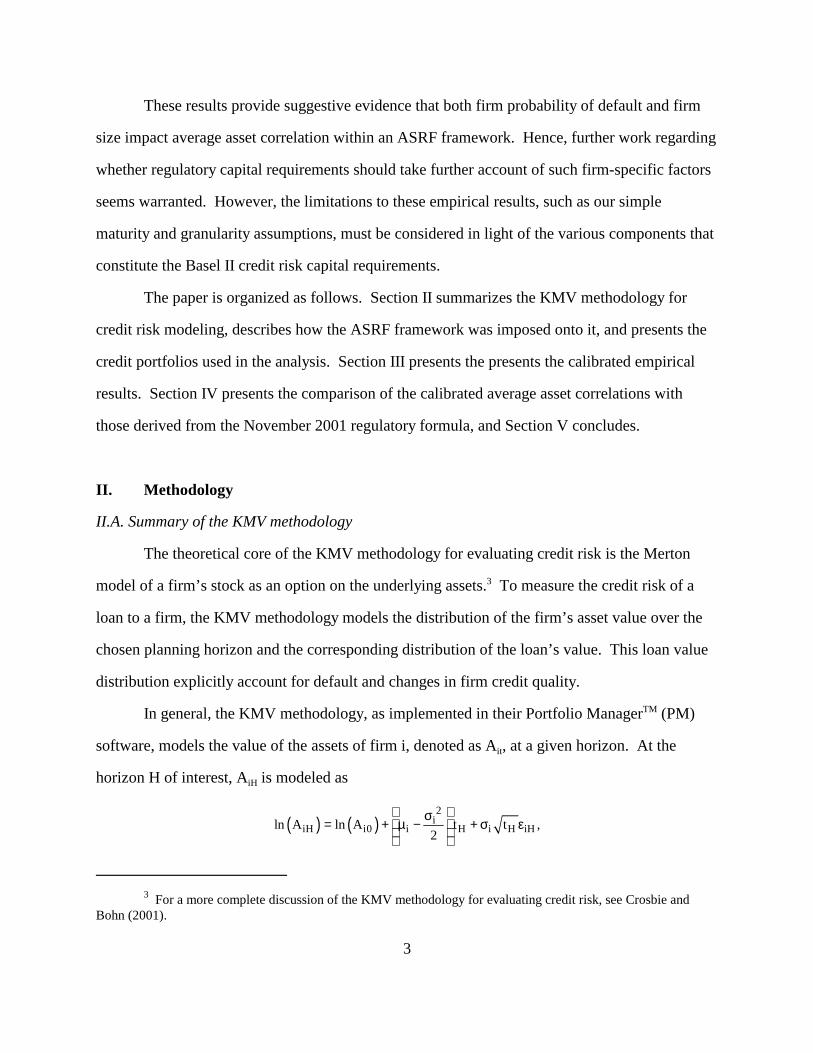
horizon H of interest, AiH is modeled as

( ) ( )2

iiH i0 i H i H iHln A ln A t t ,

2

σ = + µ − + σ ε

4

where �i is the asset value drift term (typically positive), �i2 is the firm’s asset volatility, tH is the

amount of time from period t to the horizon H, and the firm-specific error term �iH is a weighted

average of common (or systematic) random factors and an idiosyncratic random factor. That is,

�iH is modeled as

,2iH i H i iHR 1 Rε = ξ + − υ

where Ri2 measures the percentage of the firm’s asset return variance attributable to a common

risk factor, �H is a random variable representing the H-period-ahead composite risk factor, and �iH

is an idiosyncratic random variable. Both �iH and �iH have a standardized variance of one. This

decomposition of �iH ensures that it has a variance of one. Note that the Ri2 is referred to as the

asset correlation for firm i.

For each firm of interest, KMV determines its overall liabilities at time H. For a

particular realization of future asset value AiH, a “distance to default” measure is calculated and

used to determine a firm’s “expected default frequency”TM (or EDFTM) based on KMV’s

proprietary default database. The firm’s EDF value and its loans’ recovery rates permit the

calculation of the loan values if the firm defaults. For non-default states, the loans are valued by

discounting their cashflows using market-based credit spreads corresponding to the firm’s credit

quality. Individual firm calculations can be aggregated up to the portfolio level in order to

determine the distribution of loan portfolio returns, which in turn can be used for determining

economic capital allocations and other credit risk management calculations.

II.B. Application of the ASRF framework to the KMV methodology

In order to establish regulatory capital requirements applicable across institutions and

across credit risk models, the regulatory proposals currently being considered by the BCBS are

based on a very general modeling framework, known as the asymptotic single risk factor (ASRF)

approach. As described by Gordy (2001), the ASRF approach assumes that a single risk factor is

4 The impact of the assumption of infinitely granular portfolios was not part of our analysis to date. In ouranalysis, we imposed the assumption of common loan sizes across the obligors. We further assumed that thenumbers of obligors in our sample portfolios were sufficiently large for this assumption to hold. Further researchinto the validity of these assumptions is necessary.

5

responsible for credit quality movements across all obligors in an infinitely granular portfolio.4

Each obligor has a unique asset correlation Ri2 with the common risk factor, and the realization

of this factor determines the obligors’ individual outcomes. A further simplifying assumption

that is often imposed is that the obligors all have a common (or average) asset correlation with

the composite risk factor; i.e., This assumption is needed for regulatory capital2 2iR R i.= ∀

calculations in order to reduce the number of model parameters required. Within this analytic

framework, the regulatory capital requirement for a portfolio equals the sum of the regulatory

capital requirements for the individual credits. This additive property permits the “bucketing” of

credits based on certain characteristics, such as firm default probability and recovery rates. This

property of the ASRF approach clearly simplifies the allocation of regulatory capital.

To impose the ASRF approach within the KMV methodology, a number of restrictions

were imposed on the PM software. The most important restriction was imposing a single risk

factor. Within the KMV methodology, there are about 110 factors based on global, regional,

country, sector and industry effects. These various factors are aggregated based on firm

characteristics to construct a firm’s composite factor. For example, the return on the composite

factor (denoted CFi) for a U.S. domestic firm that is 60% involved in paper production and 40%

in lumber production is

CFi = 1.0 rUSA + 0.6 rpaper + 0.4 rlumber,

where rUSA, rpaper and rlumber are the returns on the factors for the entire U.S. economy, the global

paper industry and the global lumber industry, respectively. A regression of firm i’s asset returns

on the weighted average factor CFi provides the asset correlation Ri2 used in the asset value

simulations.

Thus, to impose the ASRF approach, we collapsed the many factors into a single factor

5 Within the ASRF framework, the recommended capital requirements are independent of the commonfactor chosen. However, in the empirical implementation, differences will arise when different factor specificationsare used. These differences should be minor, and preliminary results support this hypothesis.

6

common to all obligors in the credit portfolio. This restriction is imposed by forcing all of the

firms to have the same degree of dependence on the same country and industry factors. In our

analysis, we assumed that all obligors were dependent on the U.S. country factor (regardless of

their country of origin) and on the unassigned industry factor, known as N57 within the KMV

industry database.5 The common degree of dependence was imposed by assuming a common R2

value for all obligors. This common R2 value is termed the average asset correlation, even

though it is not strictly an average, and it will be denoted here as These two restrictions areA .ρ

obviously quite strong, but necessary for applying the ASRF framework.

There is no theoretical answer as to what the value of the average asset correlation should

be, and thus purely empirical values must be determined. To calibrate the empirical value of Aρ

for a portfolio at a specified loss tail quantile, we minimized the absolute difference between the

credit losses indicated by the unconstrained PM model and by the ASRF-constrained version.

The calibrations were conducted using a grid search over a reasonable range for values. TheAρ

convergence criteria used were that the calibrated values would only have up to fourAρ

significant digits and that the dollar differences between the two models’ capital charges at the

specified quantile were less than 0.1% of the total portfolio size. The calibrated valuesAρ

correlations for credit portfolios composed of firms with similar default probabilities, asset sizes

and national origin are the core contribution of this paper.

The third restriction needed to impose the ASRF framework within the PM software is

that the recovery rate is constant. For the sake of simplifying our analysis, we also imposed a

recovery rate of 50% across all obligors. Although this is a strong assumption, we know that

capital charges within the PM software for portfolios with other values are a simple multiple of

each other.

6 The number of simulations that we typically used in our analysis was 100,000 runs, which is the numberrecommended by KMV for analysis of the 99.9% tail quantile. Note that BCBS (2001b) states that the confidenceinterval to be used in setting regulatory capital requirements may be increased from 99.5% to 99.9%.

7

The fourth restriction imposed on the PM software for our analysis was a one-year

maturity for all credits. This restriction is not explicitly required by the ASRF framework. In

fact, the current average maturity assumed in BCBS (2000a) is three years. Further research on

the impact of maturity on the calibrated values derived within the ASRF approach.Aρ

II.C. The procedure for generating and analyzing the average asset correlations

The procedure for implementing the ASRF approach within the PM software and

analyzing the calibrated average asset correlations consists of three steps. The first step is to

create the portfolios of interest based on firm EDF values, firm asset sizes or both. This step is

described in detail in Section II.D. The loans to the chosen firms are then structured to have a

maturity of one year, a floating rate coupon and a common commitment size of $100 million.

These restrictions obviously impact the nature of the credit portfolios being analyzed; for

example, the standard commitment size precludes analysis of the granularity issue. Further

research into this issue is required. However, the empirical results should provide meaningful

insight into the relationships of interest.

The second step consists of running the unconstrained version of the PM software on the

constructed portfolios in order to generate the capital required at the one-year horizon for the

99.5% and 99.9% percentiles of the loss distribution.6 Of the various definitions of capital used

in the PM software, we chose to use capital in excess of expected loss. That is, PM generates the

portfolio’s credit loss distribution, designates its mean as the expected loss, and presents the tail

quantiles as credit losses beyond the expected loss. Credit losses at the one-year horizon are

transformed into capital charges by discounting them to the present with the appropriate risk-free

rate. Total capital is the sum of the discounted expect loss and the specified tail loss.

7 Note that in constructing portfolios based on EDF ranges, firms with EDF values at the ends of the rangesare included in both portfolios. For example, portfolios constructed using the second and third EDF categories havein common all firms with an EDF value exactly equal to 0.52%.

8

The third step is to calibrate the portfolios’ values as previously described. TheAρ

results for the aggregate portfolios, portfolios based on EDF categories, portfolios based on size

categories and portfolios based on both variables are then analyzed.

II.D. Credit portfolios of interest

For this study, we constructed national credit portfolios of U.S., Japanese and European

firms. The European portfolios consisted of firms based in Britain, France, Germany, Italy and

the Netherlands. We also examined aggregate (or “world”) portfolios that included all of the

firms in the national portfolios. Aside from the question of firms’ national origins, the

construction of these credit portfolios required a balance between two criteria. The first criterion

was constructing portfolios that had EDF and asset size ranges that were of economic interest.

The second criterion was insuring that the portfolios had a sufficient number of credits to avoid

small sample concerns.

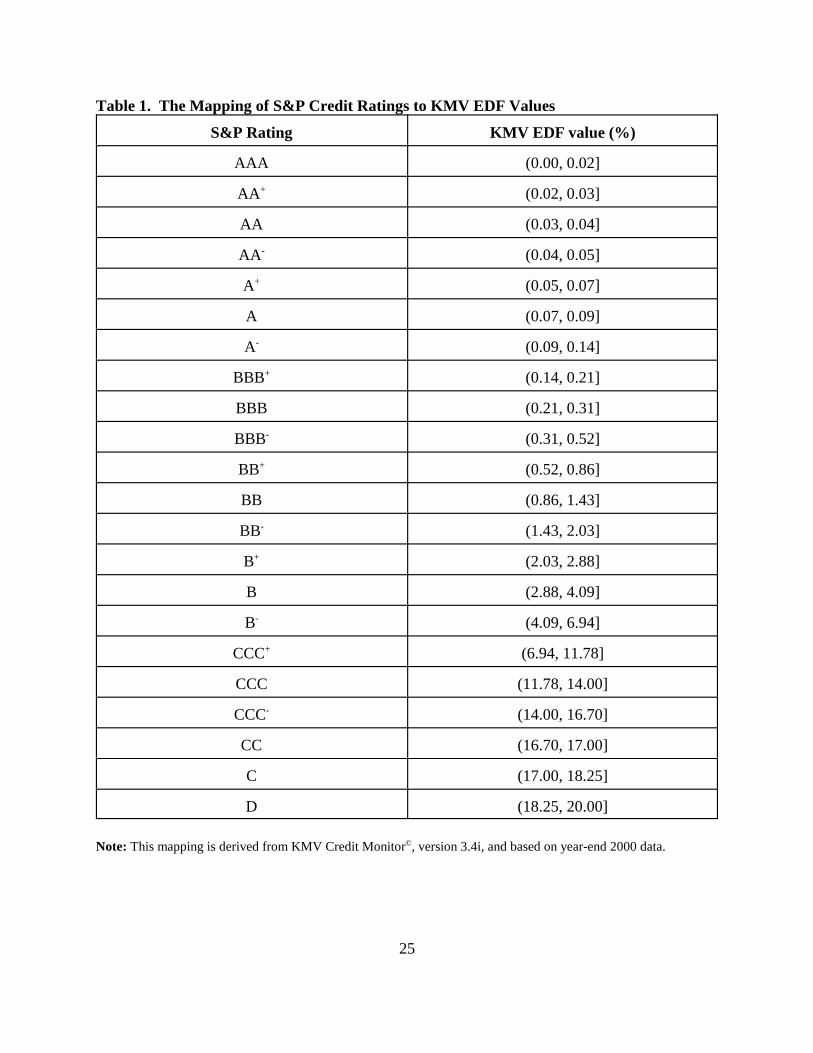
With respect to the EDFs, the portfolios were basically constructed using the S&P rating

categories set within KMV’s Credit Monitor© database as of year-end 2000; see Table 1. The

rating categories were collapsed into five EDF categories and held constant for our analysis. The

first EDF category ranged from zero to 0.05% and corresponded to AAA and AA-rated firms; the

second EDF category ranged from 0.05% to 0.52% and corresponded to A and BBB-rated firms;

the third EDF category ranged from 0.52% to 2.03% and corresponded to BB-rated firms; the

fourth EDF category ranged from 2.03% to 6.94% and corresponded to B-rated firms; and the

fifth EDF category ranged from 6.94% to 20%, the maximum EDF value permitted, and

corresponded to the remaining C and D-rated firms.7

With respect to asset size, the economic criterion for constructing portfolios was less

9

meaningful. Hence, we chose size categories that were sufficiently different to ensure that we

captured important relative size differences, but we erred on the side of making the portfolios

large enough to provide meaningful empirical results. Note that the asset size categories could

not be held constant across the national groups in a meaningful way.

With respect to the portfolios based on both EDF and size categories used in the bivariate

analysis, the challenge was to create portfolios whose numbers of credits were approximately

uniformly distributed across both sets of categories. However, this task proved impossible given

the general dearth of small firms with low EDF values and large firms with high EDF values.

Thus, for the bivariate analysis, we collapsed the previous five categories per characteristic into

three categories, which generated nine EDF and asset size portfolios for each set of firms. We

used the same three EDF categories across the sets of firms, and they were (0%, 0.52%], [0.52%,

6.94%] and [6.94%, 20.00%]. However, the size categories again varied across the sets.

III. Calibration results

The calibrated values are presented below in four subsections corresponding to theAρ

aggregate portfolios, univariate analysis of the portfolios constructed using EDF categories,

univariate analysis of the portfolios constructed using asset size categories, and bivariate analysis

of the portfolios constructed using both EDF and asset size categories. The preliminary

empirical results are presented for the 99.5% and the 99.9% tail percentiles, which are the two

tail percentiles of most common interest. Note that the discussion focuses on the latter percentile

since the results are quite similar.

III.A. Calibration results for the aggregate portfolios

As discussed in Section II.D, we constructed three sets of national firms, as well as the

superset of firms, in order to conduct our analysis. Given these four sets of obligors, we

calibrated the values for the corresponding portfolios. The results are summarized in TableAρ

8 This difficulty is endemic to the ASRF approach. As discussed by Gordy (2001), the use of a single riskfactor imposes a common business cycle on all obligors, and all other elements of credit risk are considered to beidiosyncratic. Under this construct, the average asset correlation for a heterogeneous portfolio (such as a collectionof firms from a cross-section of countries) should be lower than for a homogenous portfolio with similarcharacteristics.

10

2 and Figure 1.

For the “world” portfolio, a total of 13,839 firms were used in the exercise with about

50%, 24% and 26% being of U.S., Japanese and European origin, respectively. The calibrated

value for this portfolio was relatively low at 0.1125, potentially suggesting that a single riskAρ

factor is not sufficient to capture the heterogenous nature of the credits in the portfolio.

This possibility seems to be reinforced by the differing values for the three nationalAρ

portfolios. At the 99.9% percentile, these values are 0.1625 for the U.S. portfolio, 0.2625 for the

Japanese portfolio and 0.1375 for the European portfolio. The Japanese value is noticeably

higher than the others, probably due to the generally poor economic conditions within Japan at

year-end 2000. The European value is relatively low, suggesting that a single factor may not be

sufficient to capture the heterogeneity across the five countries that compose that portfolio. The

differing values suggest that the degree of heterogeneity across national categories of borrowers

may not be well captured by a single risk factor.8 In fact, as mentioned earlier, the unconstrained

PM model employs over 100 factors.

III.B. Univariate calibration results for portfolios based on EDF categories

Within the ASRF framework, we expect to see a negative relationship between firm asset

correlation and their probabilities of default (PD). That is, as a firm’s PD increases due to

worsening conditions and its approaching possible default, it is reasonable to think that

idiosyncratic factors begin to take on a more important role relative to the common, systematic

risk factor. The calibrated value for the portfolios based on EDF categories support thisAρ

intuition. These results are presented in Tables 3A through 3D and Figure 2A through 2D. Note

9 As noted in BCBS (2001c), a potential modification to the Basel II process is a focus on capitalrequirements set at the 99.9% percentile rather than the 99.5% percentile assumed earlier.

10 Note that the value for the 99.5% percentile for the lowest EDF category does not fit the expectedAρ

downward pattern. This result is probably due to the small sample of only 85 firms in that portfolio. Thus, the Aρ

value for the 99.9% percentile is also questionable.

11

that the results are presented for both the 99.5% and 99.9% percentiles, but the discussion

focuses on the latter set of results.9

For all firms, the results in Table 3A and Figure 2A indicate that the calibrated valuesAρ

decline, if only gradually, as the EDF values of the categories increase. For the lowest category,

the calibrated value is 0.1500, and for the highest category, it is 0.1000. However, theAρ

national portfolios show more variation in this pattern, as shown in Tables 3B through 3D and

Figures 2B through 2D.

For the U.S. portfolios, the calibrated values are higher than the world portfolios, andAρ

the slope of the decline is steeper. That is, the decline from the lowest to the highest EDF

categories is 0.0750, as opposed to 0.0500 for the world portfolios. A possible reason for this

result is that the world portfolios’ greater degree of heterogeneity lessens the impact of the EDF

decline on the calibrated values.Aρ

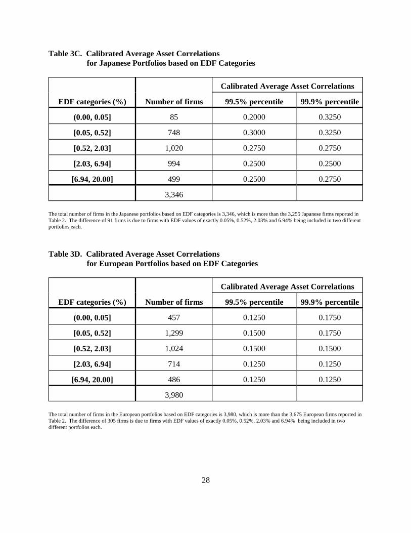
The Japanese portfolios vary the most from the other national portfolios in that the

calibrated values are higher across all EDF categories. The calibrated values range fromAρ Aρ

0.3250 to 0.2750. The decline of about 0.0500 across the categories is in line with the world and

European portfolios. Although this decline is also by 0.0500, the higher levels imply a slighter

percentage decline than for the other national portfolios. As mentioned before, the state of the

Japanese economy at year-end 2000 was such that less firm heterogeneity in condition was

possible, and this circumstance might be better explained by a single factor, even across the EDF

categories. In addition, the calibrated values for the two percentiles are different, with theAρ

values for the 99.9% percentile being higher.10

In contrast, the European portfolios have the lowest calibrated values, ranging fromAρ

11 Note that there are a wide variety of size measures available, such as total sales revenue or number ofemployees. Further research is necessary to determine the robustness of the presented results to a change in sizedefinition.

12

0.1750 to 0.1250 for the 99.9% percentile. The decline is even slighter for the 99.5% percentile,

especially given the anomalous 0.1250 value for the lowest EDF category. These lower values

are in line with the world portfolio, suggesting that the heterogeneity among the European firms

in the sample is also hard to capture with a single, common risk factor.

III.C. Univariate calibration results for portfolios based on asset size categories

In the general finance theory of portfolio diversification, as the number of different stocks

within a portfolio increases, the portfolio becomes more diversified, and the idiosyncratic

element of the portfolio’s return becomes less important. An analogous view could be taken with

respect to a firm’s asset size; that is, as a firm becomes larger and comes to contain more assets,

it’s risk and return characteristics should more closely resemble the overall asset market and be

less dependent on the idiosyncratic elements of the individual business lines. Within an ASRF

framework, this intuition suggests that a firm’s asset correlation should increase as its asset size

increases. However, this hypothesis must be verified empirically. In this paper, we tested this

hypothesis using firm asset size as the relevant size measure.11 The calibration results based on

asset size categories are presented in Table 4A through 4D and Figures 3A through 3D.

For the world portfolios based on all the firms in the three national portfolios, the

calibrated value effectively doubles from 0.1000 for firms smaller than $20 million to 0.2000Aρ

for firms larger than $1 billion. The patterns for the national portfolios are similar, but they show

certain differences.

For the U.S. portfolio, the calibrated values actually increase by more, but the rate ofAρ

increase across the size categories is more gradual. The calibrated value is 0.1000 for U.S.Aρ

firms smaller than $20 million and effectively triples to 0.3000 for firms larger than $1 billion.

13

As shown in Figure 3B, this increase is approximately linear across the chosen size categories,

while the increase for the world portfolio, as shown in Figure 3A, appears to be more exponential

in nature. A potential reason for this difference appears to be that the Japanese firms in the world

portfolio are generally of larger size than the U.S. firms. As shown in Table 4C, fewer Japanese

firms fall into asset size categories less than $100 million than U.S. firms. Approximately 20%

of the sample’s Japanese firms fall into this category, while about 44% of U.S. and European

firms in the sample fall into these categories. Since firms with assets greater than $1 billion

make up about 20% of each of the three national samples, the 24 percentage point difference for

the Japanese firms is accounted for by the category of firms between $100 million and $1 billion

in assets.

The calibrated values for the Japanese portfolios are again higher than those for theAρ

world, U.S. and European portfolios. In fact, for these size portfolios, the calibrated valuesAρ

are relatively much higher, with values of 0.2000 for firms smaller than $100 million and 0.4500

for firms larger than $1 billion, a multiple of 2.5 across the size categories. As shown in Figure

3C, the increase appears to be more exponential in nature. The Japanese portfolios are clearly

different from the U.S. and European portfolios, and hence they are probably contributing greatly

to the shape of the increases for the world portfolio.

As before, the calibrated values for the European firms are generally the lowest of theAρ

three aggregate portfolios, ranging from 0.1125 for firms smaller than $25 million and 0.2250 for

firms larger than $1 billion. The doubling of the calibrated values across the specified sizeAρ

spectrum equals that of the world portfolios and is the lowest of the national portfolios. Note

that the pattern of increases, as shown in Figure 3D, again seem to be more exponential than

linear.

III.D. Bivariate calibration results for portfolios based on EDF and asset size categories

The results discussed in the prior two sections indicate that average asset correlations

12 Note that as before, the EDF categories are common across the three national portfolios and the worldportfolio, but the asset size categories vary.

14

within an ASRF framework appear to be a decreasing function of EDF and an increasing

function of asset size. In this section, we examine whether calibrated values are a functionAρ

of both variables simultaneously. To do so, we formed nine portfolios based on both EDF and

asset size categories for the four sets of firms and determined the values that minimized theAρ

dollar difference between the capital requirements for the unconstrained PM model and the

constrained ASRF version.12

The calibration results suggest three key outcomes. First, as in the univariate results, the

calibrated average asset correlations are generally decreasing functions of EDF and increasing

functions of asset size. Thus, both of the these univariate results are important to consider.

Second, the increases in the calibrated average asset correlation with respect to increases in size

appear to be larger than the decreases with respect to increasing EDF values. In other words, the

marginal impact on a calibrated of an increase in firm asset size appears to be larger than theAρ

marginal impact of an increase in firm EDF value. Third, the changes in the calibrated valuesAρ

across EDF categories appear to become greater as firm asset size increases. That is, as firms get

larger, changes in EDF lead to larger changes in firm sensitivity to the common risk factor. A

further result is that the level rankings across the four aggregate portfolios remain the sameAρ

as for the univariate results. However, this result may not be surprising given that the data

sample period of year-end 2000 is the same.

Two important caveats regarding the calibration results in this section should be noted.

First, the analysis was conducted using discrete EDF and size categories and not using

continuous functions. Hence, any inference on changes across the categories is relativelyAρ

limited and cannot be easily tested. However, the general patterns of variation that are observed

should provide reasonably suggestive evidence. Second, the number of firms in the portfolios

varies and can be quite low in the extreme categories, such as the largest firms with highest EDF

15

values and the smallest firms with lowest EDF values. These data limitations are endemic to this

type of analysis and can effectively be seen as increasing the standard errors around the calibrated

values for those portfolios. This larger degree of uncertainty obviously limits the inferenceAρ

that can be drawn from the results. However, the general patterns discussed here should be

robust since they are also observed for portfolios that have reasonable numbers of observations.

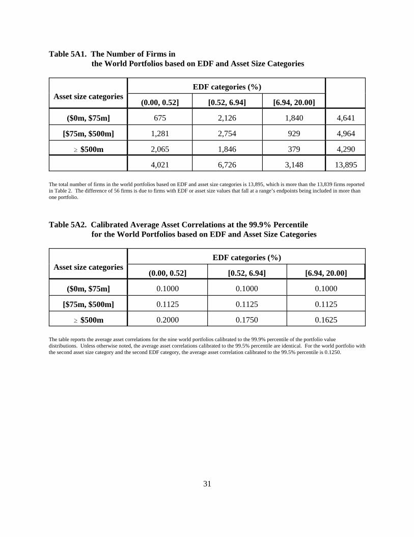
Turning to the results, the calibrated values for the nine world portfolios areAρ

presented in Table 5A and Figure 4A. Note that the values for the first two size categories do not

vary across the EDF categories, but they do decline for the third category, as previously observed.

The reasons for the constant values across the EDF categories are not clear, but this resultAρ

could be indicative that firm size is a potentially important factor in determining average asset

correlations. Looking across asset size categories for a given EDF category, we observe that the

calibrated values increase with size, as per the univariate results. For these portfolios,Aρ

variation in asset size clearly has a greater impact on the calibrated values than variation inAρ

EDF values.

The calibrated values for the nine U.S. portfolios are presented in Table 5B andAρ

Figure 4B. These values range from 0.1375 to 0.3250. Overall, these values are higher thanAρ

the values for the world portfolio, possibly indicating that national portfolio diversification issues

could impact the average asset correlations. The univariate patterns previously observed are

apparent in the bivariate analysis as well. Looking across the categories, the calibrated Aρ

values decrease from the lowest to the highest EDF categories within a given size category by

roughly 0.1000, whereas the values approximately double from the smallest to the largestAρ

size category within a given EDF category. This result further suggests the importance of firm

size in determining a portfolio’s average asset correlation.

The calibrated values for the Japanese portfolios are presented in Table 5C andAρ

Figure 4C. As noted before, the values for these portfolios are substantially higher thanAρ

those of the other national portfolios. The values range from 0.2000 to 0.5500, although this

16

latter value for the portfolio with the largest firms and the highest EDF values is based on a

sample of just 64 firms (or just 2% of the Japanese sample). Although the pattern of declining

values within a size category due to increasing EDF values is not apparent here, the Aρ Aρ

values do increase with asset size for a given EDF category. In fact, the size effect is strongest

for the Japanese results.

The calibrated values for the European portfolios are presented in Table 5D andAρ

Figure 4D. The values here range from 0.1250 to 0.2000. Note that these values do not vary

much across either EDF or asset size categories. In fact, = 0.1250 for all EDF categoriesAρ

across the first two asset size categories. Only for the largest EDF category do we observe an

increase in across the size categories and a decline across the EDF categories. This relativeAρ

lack of variation is approximately similar to the univariate results, but further analysis isAρ

needed here.

In conclusion, the analysis of the calibrated values using an ASRF framework withinAρ

the KMV methodology provides strong suggestive evidence that both EDF values and firm size

are important driving factors. In addition, the results also suggest national characteristics are

potentially important, but more analysis over other time periods is necessary to verify this result.

IV. Regulatory Values for Average Asset Correlation

In an effort to update and improve international bank capital requirements, the BCBS

began a revision of the 1988 Basel Accord in 1999, a process that has come to be known as

“Basel II”. A primary goal of the Basel II process is to make credit risk capital requirements

more risk-sensitive; i.e., more closely linked to the economic risks faced by banks in their

business activities. Credit risk modeling is to play an important role in this process.

As detailed in BCBS (2001a), the BCBS decided to adopt an evolutionary approach to the

implementation of credit risk capital requirements, an approach that mirrors the evolution of

13 For a survey of the credit risk modeling at large financial institutions, see BCBS (1999). See Hirtle et.al(2001) for a discussion of the policy options for using such models for regulatory purposes,

17

credit risk management techniques themselves.13 For banks that do not have sufficiently well

developed credit risk models, credit risk capital requirements are to be determined using the

“standardized” approach, which effectively does not require modeling input from the banks.

However, for banks that are employing more quantitatively oriented techniques of credit risk

management, particularly internal risk-rating systems, an internal-ratings based (IRB) approach

was proposed.

The IRB approach has two tiers within it. The first tier, known as the “foundation” IRB

approach, permits banks to input their own credit risk assessments of their lending portfolios, but

estimation of additional inputs are derived through the application of standardized regulatory

rules. This IRB approach is intended to be used by banks that currently face difficulty in

estimating certain risk model parameters due to data limitations or less-developed credit risk

models. The second tier, known as the “advanced” IRB approach, would allow banks to use their

own internal credit risk modeling outcomes to establish their regulatory credit risk capital

requirements.

As mentioned earlier, the analytical framework used for determining credit risk capital

requirements within the Basel II process is the ASRF framework described by Gordy (2001).

Within this framework, as discussed in section II, the average asset correlation is a keyAρ

parameter, but regulators need only specify a value for it for the foundation IRB approach. In

paragraph 172 of the January 2001 proposal (BCBS, 2001a), the regulatory value of was setAρ

to be constant at 0.2000, based on surveys of industry practice and research conducted by the

BCBS.

This assumption, as well as the various others that compose the IRB approach, were

examined within the context of two quantitative impact studies; the second of which, known as

QIS-2, was initiated in April 2001 and summarized in BCBS (2001c). In light of those results,

14 The BCBS clearly states that it “has not at this stage endorsed the specific modifications that are thefocus of the additional quantitative impact exercise.”

18

the BCBS initiated a more targeted study of the foundation IRB approach in November 2001,

which is known as QIS-2.5; see BCBS (2001b).14 Within this study, the asset correlation

assumption was modified to make �A a function of the probability of default (PD). Specifically,

( )50 PD 50 PD

A 50 50

1 e 1 ePD 0.10 0.20 1 ,

1 e 1 e

− ∗ − ∗

− −

− −ρ = + − − −

or equivalently,

( )50*PD

A 50

1 ePD 0.2 0.1 .

1 e

−

−

−ρ = − −

See Figure 5 for a graphical presentation of this function.

In this section, we further analyze our calibrated values with respect to both theAρ

proposed January and November regulatory values. Specifically, the calibrated valuesAρ Aρ

are compared to the assumption that and to the November proposal evaluated atA 0.2000ρ =

the mean, median and maximum EDF values of the constructed portfolios. Note that only the

median results will be addressed directly. The results are presented in Tables 6 through 9 and

Figures 6 through 9.

These results suggest five key outcomes. First, the overall comparison of the calibrated

values and the January proposal suggests that there is sufficient variation as to make theAρ

constant assumption too inaccurate. Second, the overall comparison of the calibrated valuesAρ

and the November proposal are rather favorable, especially for higher EDF categories and more

diversified portfolios. However, there are important areas of difference. Third, limitation to a

maximum �A(PD) value of 0.2000 is not warranted by the calibration results. Fourth, the decline

in �A(PD) due to increases in PD values is quicker than suggested by the calibrated values. Aρ

19

Fifth, the formula in the November proposal does not account for size, and the greatest

deviations from the calibrated values are for the larger firms, suggesting the potential valueAρ

of incorporating some element of firm size into the regulatory values for average asset

correlations.

IV.A. Comparison for aggregate portfolios

The comparison of the calibrated values for the four aggregate portfolios with theAρ

November regulatory values is presented in Table 6 and Figure 5. Overall, the calibrated Aρ

values are not that different, with the exception of the Japanese portfolio. The calibrated Aρ

value for this portfolio is 0.2625, while the November regulatory proposal suggests a value of

0.1430, which is more in line with the value for the regulatory values of the other three

portfolios. These results suggest that for broadly diversified portfolios, the November proposal

for regulatory values appears to match the calibration results quite well, although countryAρ

concentrations may be a concern.

IV.B. Comparison for portfolios based on EDF categories

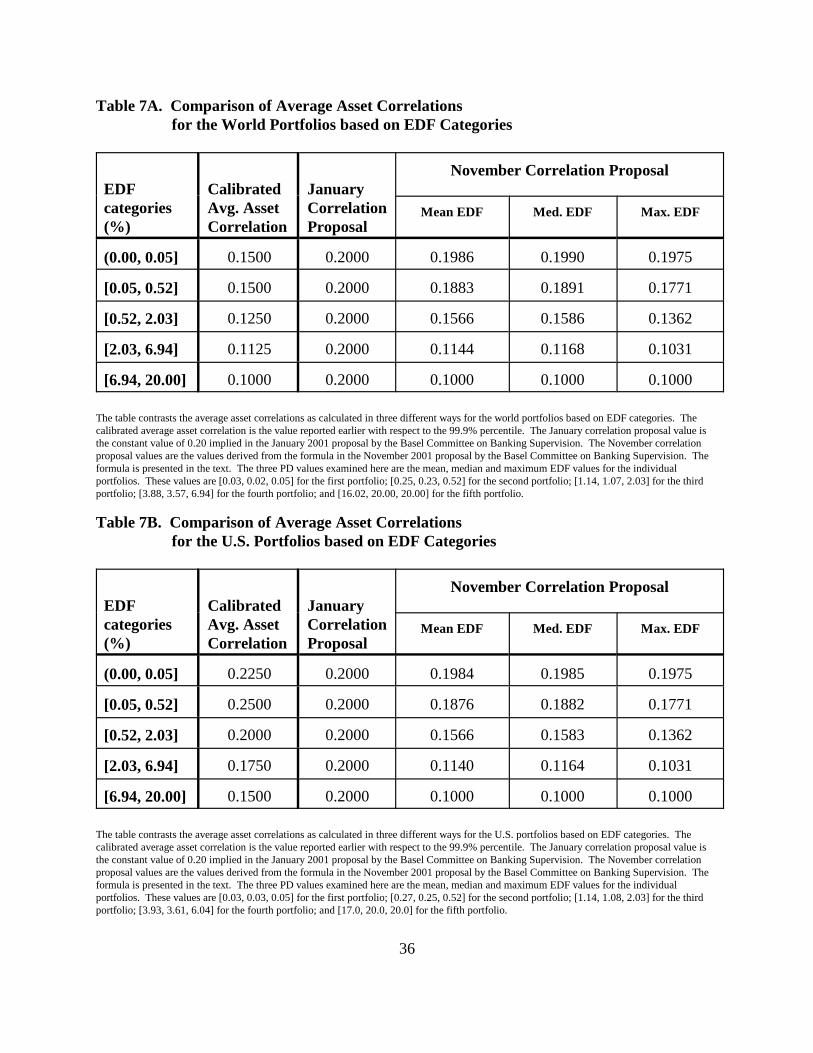
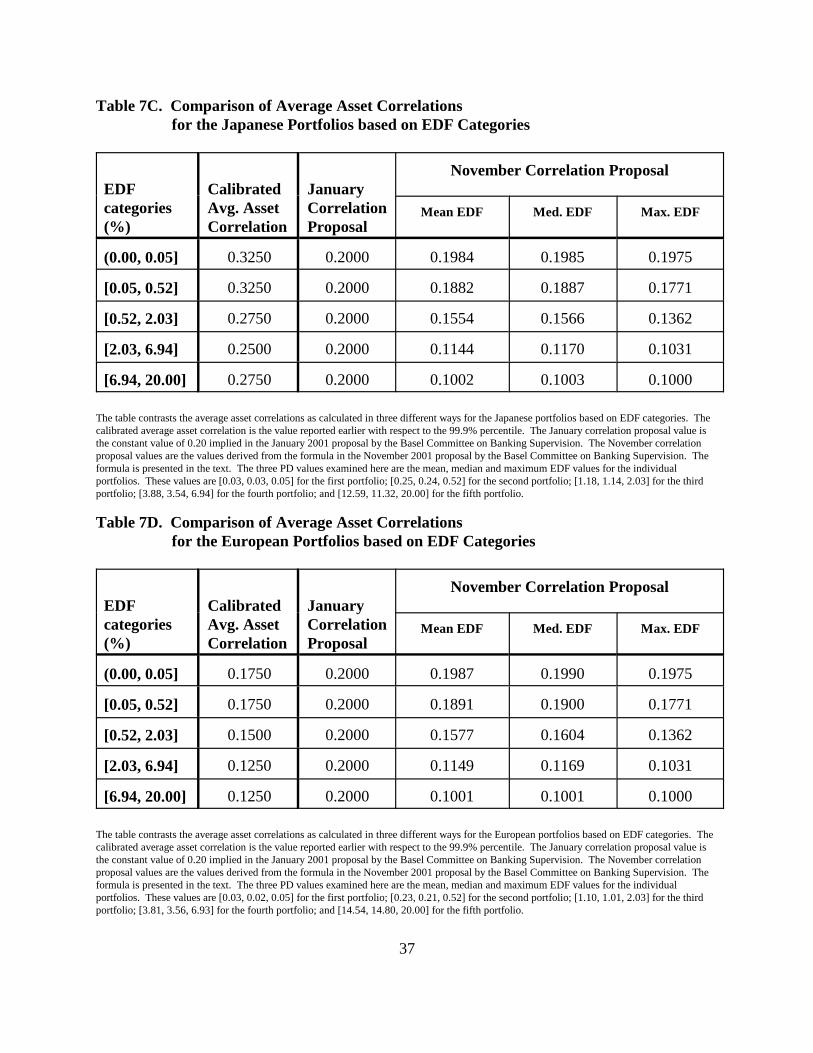
The comparison of calibrated values for the portfolios based on EDF categories withAρ

the November regulatory proposal evaluated at the portfolio medians is presented in Tables 7A

through 7D and Figure 6. Overall, the differences between these alternative values isAρ

relatively small, again except for the Japanese portfolios. Using the metric that deviations of

±0.05 are reasonable, the calibrated values for the world, U.S. and European portfolios areAρ

well represented by the November regulatory values. The calibrated values for the JapaneseAρ

portfolio range from 0.2500 to 0.3250, all of which exceed the maximum regulatory value. Note

that several U.S. portfolios with smaller median EDF values also have calibrated valuesAρ

above 0.2000.

Another interesting point of comparison is the speed with which the alternative Aρ

20

values decline as EDF increases. Of course, the alternative measures are difficult to compare

since one is calibrated for select EDF ranges and the other is a continuous PD function.

However, the comparative results in Table 7 suggest that the regulatory values decline at aAρ

slightly faster rate than suggested by the calibrated values.Aρ

IV.C. Comparison for portfolios based on asset size categories

The comparison between the calibrated values for the portfolios based on asset sizeAρ

categories and the values from the November regulatory proposal evaluated at the portfolio

medians is presented in Tables 8A through 8D and Figure 7. As the November proposal does not

incorporate a measure of firm size, the regulatory values in this table do not account for theAρ

size variation across portfolios. However, they increase across the size categories, as observed in

previous sections, because the median EDF values of the portfolios also increase with asset size.

Overall, the differences between the alternative values is relatively small (i.e., withinAρ

a range of ±0.05), with the main exception of the Japanese portfolios. As before, the Japanese

calibrated values are much larger than the regulatory values, with differences rangingAρ Aρ

from 0.07 to 0.28. Another exception was the second size category for the European portfolios,

and two further exceptions were observed here for the two largest categories of U.S. firms. The

calibrated values exceeded the regulatory maximum value and had differences of more than 0.05.

Thus, although the regulatory values are quite similar to the calibrated values, the U.S.

exceptions could suggest that important deviations due to firm size, especially for large firms,

may be a concern.

IV.D. Comparison for portfolios based on EDF and asset size categories

The comparison of calibrated values for the portfolios based on EDF and asset sizeAρ

categories with the regulatory values based on the November proposal evaluated at the portfolio

medians is presented in Tables 9A through 9D and Figures 9A through 9D. As before, the

21

regulatory values increase across the asset size categories for a given EDF category becauseAρ

of the increasing median EDF values, but these increases are moderated relative to the results in

Table 8 due to the smaller sample sizes in the bivariate analysis.

Overall, the differences between the alternative measures are once again relatively small;

i.e., within ±0.05. Of the 36 portfolios examined, the absolute difference in values wasAρ

greater than 0.05 for 47% of the cases and just 37% when the Japanese portfolios are excluded.

The deviations were largest for firms in the largest size categories, which accounted for 50% of

the deviations excluding the Japanese portfolios. These results suggest that the calibrated Aρ

values deviate most from the regulatory values, which do not take size into account, for the

largest firms in the four firm samples.

The results in Table 9 show that the speeds with which the alternative values declineAρ

as the EDF values increases are quite different. Within an asset size category, the calibrated Aρ

values generally either remain constant or decline moderately as the median EDF values increase

across the EDF categories, again with the exception of the Japanese portfolios. However, for the

regulatory values, the values start near the maximum value of 0.2000 for the lowest EDFAρ

category and quickly dive to the minimum value of 0.1000. Thus, by ignoring firm asset size, the

regulatory proposal causes greater variability than is suggested by the calibrated values. Aρ Aρ

These results further suggest that a consideration of firm asset size in the calculation of the

regulatory values, especially for larger firms, could be warranted.Aρ

V. Conclusion

The asymptotic single risk factor (ASRF) approach is a simplifying framework for

determining regulatory capital charges for credit risk. As described by Gordy (2001), this

framework has become the basis upon which the credit risk capital charges for the second Basel

Accord are being determined. In this paper, the ASRF approach was imposed on the KMV

methodology for determining credit risk capital charges in order to examine the relationship

22

between average asset correlation, firm probability of default and firm asset size measured by the

book value of assets. The analysis was conducted on national portfolios of American, Japanese

and European firms, as well as a world portfolio composed of the three national portfolios, using

data from year-end 2000.

The univariate calibration results indicate that average asset correlation is a decreasing

function of the probability of default. This univariate result suggests that the reasons why firms

experience rising default probabilities are mainly idiosyncratic and not as closely tied to the

general economic environment summarized by the single, common factor. The empirical results

further indicate that average asset correlation is increasing in asset size. That is, as firms increase

the book value of their assets, they become more correlated with the general economic

environment and the common factor. This result is intuitive in the sense that larger firms can

generally be viewed as portfolios of smaller firms, and such portfolios would be relatively more

sensitive to common risks than to idiosyncratic risks.

The bivariate calibration results support both sets of univariate results and appear to

highlight an additional and potentially important relationship between the three variables. The

decreasing relationship between average asset correlation and default probability is more

pronounced for larger firms. In other words, the average asset correlation for larger firms is more

sensitive to firm probability of default than it is for smaller firms. These results provide evidence

that both default probability and firm size impact average asset correlation within an ASRF

framework, especially for larger firms. Hence, further work regarding whether regulatory capital

requirements should take account of other factors seem warranted.

In this paper, we also compared the calibration results with the formula for the average

asset correlation proposed by the BCBS in November 2001. This formula explicitly makes the

average asset correlation a function of firm probability of default. Based on the regulatory

formula, the deviations between the calibrated and regulatory values that are greatest are forAρ

the larger firms, suggesting the potential value of incorporating firm size into the regulatory

23

average asset correlation formula.

These calibration results provide suggestive evidence that firm size is an important

variable in determining credit risk capital requirements and may need to be accounted for in the

regulatory calculations within the Basel II process. However, the limitations to these calibration

results, such as the simple maturity and granularity assumptions, must be considered in light of

all the elements of the Basel II credit risk capital requirements, and the final regulatory capital

requirements may not need to explicitly account for these relationships within the average asset

correlation.

24

References

Basel Committee on Banking Supervision, 1999. “Credit Risk Modeling: Current Practices andApplications,” Technical report, Bank for International Settlements.

Basel Committee on Banking Supervision, 2001a. “The Internal Ratings-Based Approach:Supporting Document to the New Basel Capital Accord,” Consultative document.

Basel Committee on Banking Supervision, 2001b. “Results of the Second Quantitative ImpactStudy,” Press release dated November 5, 2001.

Basel Committee on Banking Supervision, 2001c. “Potential Modification to the Committee’sProposals,” Press release dated November 5, 2001.

Crosbie, P.J. and Bohn, J.R., 2001. “Modeling Default Risk,” Manuscript, KMV LLC. (http://www.kmv.com/Knowledge_Base/public/cm/white/Modeling_Default_Risk.pdf)

Gordy, M.B., 2000a. “A Comparative Anatomy of Credit Risk Models,” Journal of Banking andFinance, 24, 119-149.

Gordy, M.B., 2000b. “Credit VAR and Risk-Bucket Capital Rules: A Reconciliation,” inProceedings of the 36th Annual Conference on Bank Structure and Competition, 406-415.

Gordy, M.B., 2001. “A Risk-Factor Model Foundation for Ratings-Based Bank Capital Rules,”Manuscript, Board of Governors of the Federal Reserve System.

Hirtle, B., Levonian, M., Saidenberg, M., Walter, S. and Wright, D., 2001. “Using Credit RiskModels for Regulatory Capital: Issues and Options,” Federal Reserve Bank of New YorkEconomic Policy Review, March, 19-36.

25

Table 1. The Mapping of S&P Credit Ratings to KMV EDF Values

S&P Rating KMV EDF value (%)

AAA (0.00, 0.02]

AA+ (0.02, 0.03]

AA (0.03, 0.04]

AA- (0.04, 0.05]

A+ (0.05, 0.07]

A (0.07, 0.09]

A- (0.09, 0.14]

BBB+ (0.14, 0.21]

BBB (0.21, 0.31]

BBB- (0.31, 0.52]

BB+ (0.52, 0.86]

BB (0.86, 1.43]

BB- (1.43, 2.03]

B+ (2.03, 2.88]

B (2.88, 4.09]

B- (4.09, 6.94]

CCC+ (6.94, 11.78]

CCC (11.78, 14.00]

CCC- (14.00, 16.70]

CC (16.70, 17.00]

C (17.00, 18.25]

D (18.25, 20.00]

Note: This mapping is derived from KMV Credit Monitor©, version 3.4i, and based on year-end 2000 data.

26

Table 2. Calibrated Average Asset Correlations for Aggregate Portfolios

Calibrated Average Asset Correlations

Portfolio Number of firms 99.5% percentile 99.9% percentile

All firms 13,839 0.1125 0.1125

U.S. firms 6,909 0.1625 0.1625

Japanese firms 3,255 0.2625 0.2625

European firms 3,675 0.1250 0.1375

The portfolio of all firms contains all of the U.S., Japanese and European firms in the KMV CreditMonitor database as of year-end 2000. European firms are defined here as firms headquartered in France, Germany, Great Britain, Italy and the Netherlands. Note that U.S., Japaneseand European firms make up 50%, 24% and 26%, respectively, of all the firms examined here.

27

Table 3A. Calibrated Average Asset Correlations for World Portfolios based on EDF Categories


EDF categories (%) Number of firms 99.5% percentile 99.9% percentile

(0.00, 0.05] 644 0.1500 0.1500

[0.05, 0.52] 3,478 0.1500 0.1500

[0.52, 2.03] 3,711 0.1250 0.1250

[2.03, 6.94] 3,034 0.1125 0.1125

[6.94, 20.00] 3,148 0.1000 0.1000

14,015

The total number of firms in the world portfolios based on EDF categories is 14,015, which is more than the 13,839 firms reported in Table 2. The difference of 176 firms is due to firms with EDF values of exactly 0.05%, 0.52%, 2.03% and 6.94% being included in two differentportfolios each.

Table 3B. Calibrated Average Asset Correlations for U.S. Portfolios based on EDF Categories



(0.00, 0.05] 131 0.2250 0.2250

[0.05, 0.52] 1,567 0.2250 0.2500

[0.52, 2.03] 1,798 0.2000 0.2000

[2.03, 6.94] 1,437 0.1750 0.1750

[6.94, 20.00] 2,475 0.1500 0.1500

7,408

The total number of firms in the U.S. portfolios based on EDF categories is 7,408, which is more than the 6,909 U.S. firms reported in Table 2. The difference of 499 firms is due to firms with EDF values of exactly 0.05%, 0.52%, 2.03% and 6.94% being included in two differentportfolios each.

28

Table 3C. Calibrated Average Asset Correlations for Japanese Portfolios based on EDF Categories



(0.00, 0.05] 85 0.2000 0.3250

[0.05, 0.52] 748 0.3000 0.3250

[0.52, 2.03] 1,020 0.2750 0.2750

[2.03, 6.94] 994 0.2500 0.2500

[6.94, 20.00] 499 0.2500 0.2750

3,346

The total number of firms in the Japanese portfolios based on EDF categories is 3,346, which is more than the 3,255 Japanese firms reported inTable 2. The difference of 91 firms is due to firms with EDF values of exactly 0.05%, 0.52%, 2.03% and 6.94% being included in two differentportfolios each.

Table 3D. Calibrated Average Asset Correlations for European Portfolios based on EDF Categories



(0.00, 0.05] 457 0.1250 0.1750

[0.05, 0.52] 1,299 0.1500 0.1750

[0.52, 2.03] 1,024 0.1500 0.1500

[2.03, 6.94] 714 0.1250 0.1250

[6.94, 20.00] 486 0.1250 0.1250

3,980

The total number of firms in the European portfolios based on EDF categories is 3,980, which is more than the 3,675 European firms reported inTable 2. The difference of 305 firms is due to firms with EDF values of exactly 0.05%, 0.52%, 2.03% and 6.94% being included in twodifferent portfolios each.

29

Table 4A. Calibrated Average Asset Correlations for World Portfolios based on Asset Size Categories


Asset size categories Number of firms 99.5% percentile 99.9% percentile

($0 , $20m] 2,103 0.1000 0.1000

[$20m, $100m] 3,230 0.1000 0.1000

[$100m, $300m] 3,031 0.1125 0.1125

[$300m, $1,000m] 2,706 0.1375 0.1375

� $1,000m 2,969 0.2000 0.2000

14,039

The total number of firms in the world portfolios based on asset size categories is 14,039, which is more than the 13,839 firms reported in Table2. The difference of 200 firms is due to firms with asset size values of exactly $20m, $100m, $300m and $1,000m being included in twodifferent portfolios each.

Table 4B. Calibrated Average Asset Correlations for U.S. Portfolios based on Asset Size Categories



($0 , $20m] 1,515 0.1250 0.1000

[$20m, $100m] 1,655 0.1500 0.1500

[$100m, $300m] 1,330 0.1750 0.1750

[$300m, $1,000m] 1,336 0.2250 0.2250

� $1,000m 1,543 0.2750 0.3000

7,374

The total number of firms in the U.S. portfolios based on asset size categories is 7,374, which is more than the 6,909 U.S. firms reported in Table2. The difference of 465 firms is due to firms with asset sizes values of exactly $20m, $100m, $300m and $1,000m being included in twodifferent portfolios each.

30

Table 4C. Calibrated Average Asset Correlations for Japanese Portfolios based on Asset Size Categories



($0 , $100m] 643 0.2000 0.2000

[$100m, $200m] 658 0.2000 0.2000

[$200m, $400m] 633 0.2500 0.2500

[$400m, $1,000m] 606 0.3000 0.3000

� $1,000m 771 0.4250 0.4500

3,311

The total number of firms in the Japanese portfolios based on asset size categories is 3,311, which is more than the 3,255 Japanese firms reportedin Table 2. The difference of 56 firms is due to firms with asset size values of exactly $100m, $200m, $400m and $1,000m being included intwo different portfolios each.

Table 4D. Calibrated Average Asset Correlations for European Portfolios based on Asset Size Categories



($0 , $25m] 948 0.1125 0.1125

[$25m, $75m] 778 0.1125 0.1125

[$75m, $200m] 705 0.1250 0.1250

[$200m, $1,000m] 782 0.1500 0.1500

� $1,000m 693 0.2250 0.2250

3,906

The total number of firms in the European portfolios based on asset size categories is 3,906, which is more than the 3,675 European firmsreported in Table 2. The difference of 231 firms is due to firms with asset sizes values of exactly $25m, $75m, $200m and $1,000m beingincluded in two different portfolios each.

31

Table 5A1. The Number of Firms in the World Portfolios based on EDF and Asset Size Categories

Asset size categoriesEDF categories (%)

(0.00, 0.52] [0.52, 6.94] [6.94, 20.00]

($0m, $75m] 675 2,126 1,840 4,641

[$75m, $500m] 1,281 2,754 929 4,964

� $500m 2,065 1,846 379 4,290

4,021 6,726 3,148 13,895

The total number of firms in the world portfolios based on EDF and asset size categories is 13,895, which is more than the 13,839 firms reportedin Table 2. The difference of 56 firms is due to firms with EDF or asset size values that fall at a range’s endpoints being included in more thanone portfolio.

Table 5A2. Calibrated Average Asset Correlations at the 99.9% Percentile for the World Portfolios based on EDF and Asset Size Categories


(0.00, 0.52] [0.52, 6.94] [6.94, 20.00]

($0m, $75m] 0.1000 0.1000 0.1000

[$75m, $500m] 0.1125 0.1125 0.1125

� $500m 0.2000 0.1750 0.1625

The table reports the average asset correlations for the nine world portfolios calibrated to the 99.9% percentile of the portfolio valuedistributions. Unless otherwise noted, the average asset correlations calibrated to the 99.5% percentile are identical. For the world portfolio withthe second asset size category and the second EDF category, the average asset correlation calibrated to the 99.5% percentile is 0.1250.

32

Table 5B1. The Number of Firms in the U.S. Portfolios based on EDF and Asset Size Categories


(0.00, 0.52] [0.52, 6.94] [6.94, 20.00]

($0m, $100m] 230 1,214 1,734 3,178

[$100m, $1,000m] 681 1,376 606 2,663

� $1,000m 785 632 134 1,551

1,696 3,222 2,474 7,392

The total number of firms in the U.S. portfolios based on EDF and asset size categories is 7,392, which is more than the 6,909 U.S. firmsreported in Table 2. The difference of 483 firms is due to firms with EDF or asset sizes values that fall at a range’s endpoints being included inmore than one portfolio.

Table 5B2. Calibrated Average Asset Correlations at the 99.9% Percentile for the U.S. Portfolios based on EDF and Asset Size Categories


(0.00, 0.52] [0.52, 6.94] [6.94, 20.00]

($0m, $100m] 0.1375 0.1250 0.1250

[$100m, $1,000m] 0.1875 0.1875 0.1750

� $1,000m 0.3250 0.2750 0.2250

The table reports the average asset correlations for the nine U.S. portfolios calibrated to the 99.9% percentile of the portfolio value distributions. Unless otherwise noted, the average asset correlations calibrated to the 99.5% percentile are identical.

33

Table 5C1. The Number of Firms in the Japanese Portfolios based on EDF and Asset Size Categories


(0.00, 0.52] [0.52, 6.94] [6.94, 20.00]

($0m, $200m] 198 843 243 1,284

[$200m, $1,000m] 251 797 179 1,227

� $1,000m 354 340 64 758

803 1980 486 3,269

The total number of firms in the Japanese portfolios based on EDF and asset size categories is 3,269, which is more than the 3,255 Japanesefirms reported in Table 2. The difference of 14 firms is due to firms with EDF or asset sizes values that fall at a range’s endpoints beingincluded in more than one portfolio.

Table 5C2. Calibrated Average Asset Correlations at the 99.9% Percentile for the Japanese Portfolios based on EDF and Asset Size Categories


(0.00, 0.52] [0.52, 6.94] [6.94, 20.00]

($0m, $200m] 0.2250 0.2000 0.2000

[$200m, $1,000m] 0.2500 0.2500 0.2750

� $1,000m 0.4250 0.4000 0.5500

The table reports the average asset correlations for the nine Japanese portfolios calibrated to the 99.9% percentile of the portfolio valuedistributions. Unless otherwise noted, the average asset correlations calibrated to the 99.5% percentile are identical. For the Japanese portfolioconsisting of firms with asset sizes of greater than or equal to $200 million and less than or equal to $1,000 million and EDF values between0.00% and 0.52%, the average asset correlation calibrated to the 99.5% percentile is 0.2250. For the Japanese portfolio consisting of firms withasset sizes of greater than or equal to $100 million and EDF values between 6.94% and 20.00%, the average asset correlation calibrated to the99.5% percentile is 0.4250, which is lower than the value for the 99.9% percentile.

34

Table 5D1. The Number of Firms in the European Portfolios based on EDF and Asset Size Categories


(0.00, 0.52] [0.52, 6.94] [6.94, 20.00]

($0m, $25m] 207 479 197 883

[$25m, $200m] 519 714 168 1,401

� $200m 887 467 53 1,407

1,613 1,660 418 3,691

The total number of firms in the European portfolios based on EDF and asset size categories is 3,691, which is more than the 3,675 Europeanfirms reported in Table 2. The difference of 16 firms is due to firms with EDF or asset sizes values that fall at a range’s endpoints beingincluded in more than one portfolio.

Table 5D2. Calibrated Average Asset Correlations at the 99.9% Percentile for the European Portfolios based on EDF and Asset Size Categories


(0.00, 0.52] [0.52, 6.94] [6.94, 20.00]

($0m, $25m] 0.1250 0.1250 0.1250

[$25m, $200m] 0.1250 0.1250 0.1250

� $200m 0.2000 0.1750 0.1750

The table reports the average asset correlations for the nine European portfolios calibrated to the 99.9% percentile of the portfolio valuedistributions. Unless otherwise noted, the average asset correlations calibrated to the 99.5% percentile are identical.

35

Table 6. Comparison of Average Asset Correlations for the Aggregate Portfolios

Portfolio

CalibratedAvg. AssetCorrelation

JanuaryCorrelationProposal

November Correlation Proposal

Mean EDF Med. EDF Max. EDF

All firms 0.1125 0.2000 0.1082 0.1445 0.1000

U.S. firms 0.1625 0.2000 0.1033 0.1300 0.1000

Japanesefirms

0.2625 0.2000 0.1176 0.1430 0.1000

Europeanfirms

0.1375 0.2000 0.1238 0.1684 0.1000

The table contrasts the average asset correlations as calculated in three different ways for the aggregate portfolios. The calibrated average assetcorrelation is the value reported earlier with respect to the 99.9% percentile. The January correlation proposal value is the constant value of 0.20implied in the January 2001 proposal by the Basel Committee on Banking Supervision. The November correlation proposal values are thevalues derived from the formula in the November 2001 proposal by the Basel Committee on Banking Supervision. The formula is presented inthe text. The three PD values examined here are the mean, median and maximum EDF values for the individual portfolios. These values are[5.0, 1.6, 20.0] for all firms; [6.8, 2.4, 20.0] for U.S. firms; [3.5, 1.7, 20.0] for Japanese firms; and [2.9, 1.8, 20.0] for European firms.

36

Table 7A. Comparison of Average Asset Correlations for the World Portfolios based on EDF Categories

EDFcategories(%)





(0.00, 0.05] 0.1500 0.2000 0.1986 0.1990 0.1975

[0.05, 0.52] 0.1500 0.2000 0.1883 0.1891 0.1771

[0.52, 2.03] 0.1250 0.2000 0.1566 0.1586 0.1362

[2.03, 6.94] 0.1125 0.2000 0.1144 0.1168 0.1031

[6.94, 20.00] 0.1000 0.2000 0.1000 0.1000 0.1000

The table contrasts the average asset correlations as calculated in three different ways for the world portfolios based on EDF categories. Thecalibrated average asset correlation is the value reported earlier with respect to the 99.9% percentile. The January correlation proposal value isthe constant value of 0.20 implied in the January 2001 proposal by the Basel Committee on Banking Supervision. The November correlationproposal values are the values derived from the formula in the November 2001 proposal by the Basel Committee on Banking Supervision. Theformula is presented in the text. The three PD values examined here are the mean, median and maximum EDF values for the individualportfolios. These values are [0.03, 0.02, 0.05] for the first portfolio; [0.25, 0.23, 0.52] for the second portfolio; [1.14, 1.07, 2.03] for the thirdportfolio; [3.88, 3.57, 6.94] for the fourth portfolio; and [16.02, 20.00, 20.00] for the fifth portfolio.

Table 7B. Comparison of Average Asset Correlations for the U.S. Portfolios based on EDF Categories

EDFcategories(%)





(0.00, 0.05] 0.2250 0.2000 0.1984 0.1985 0.1975

[0.05, 0.52] 0.2500 0.2000 0.1876 0.1882 0.1771

[0.52, 2.03] 0.2000 0.2000 0.1566 0.1583 0.1362

[2.03, 6.94] 0.1750 0.2000 0.1140 0.1164 0.1031

[6.94, 20.00] 0.1500 0.2000 0.1000 0.1000 0.1000

The table contrasts the average asset correlations as calculated in three different ways for the U.S. portfolios based on EDF categories. Thecalibrated average asset correlation is the value reported earlier with respect to the 99.9% percentile. The January correlation proposal value isthe constant value of 0.20 implied in the January 2001 proposal by the Basel Committee on Banking Supervision. The November correlationproposal values are the values derived from the formula in the November 2001 proposal by the Basel Committee on Banking Supervision. Theformula is presented in the text. The three PD values examined here are the mean, median and maximum EDF values for the individualportfolios. These values are [0.03, 0.03, 0.05] for the first portfolio; [0.27, 0.25, 0.52] for the second portfolio; [1.14, 1.08, 2.03] for the thirdportfolio; [3.93, 3.61, 6.04] for the fourth portfolio; and [17.0, 20.0, 20.0] for the fifth portfolio.

37

Table 7C. Comparison of Average Asset Correlations for the Japanese Portfolios based on EDF Categories

EDFcategories(%)





(0.00, 0.05] 0.3250 0.2000 0.1984 0.1985 0.1975

[0.05, 0.52] 0.3250 0.2000 0.1882 0.1887 0.1771

[0.52, 2.03] 0.2750 0.2000 0.1554 0.1566 0.1362

[2.03, 6.94] 0.2500 0.2000 0.1144 0.1170 0.1031

[6.94, 20.00] 0.2750 0.2000 0.1002 0.1003 0.1000

The table contrasts the average asset correlations as calculated in three different ways for the Japanese portfolios based on EDF categories. Thecalibrated average asset correlation is the value reported earlier with respect to the 99.9% percentile. The January correlation proposal value isthe constant value of 0.20 implied in the January 2001 proposal by the Basel Committee on Banking Supervision. The November correlationproposal values are the values derived from the formula in the November 2001 proposal by the Basel Committee on Banking Supervision. Theformula is presented in the text. The three PD values examined here are the mean, median and maximum EDF values for the individualportfolios. These values are [0.03, 0.03, 0.05] for the first portfolio; [0.25, 0.24, 0.52] for the second portfolio; [1.18, 1.14, 2.03] for the thirdportfolio; [3.88, 3.54, 6.94] for the fourth portfolio; and [12.59, 11.32, 20.00] for the fifth portfolio.

Table 7D. Comparison of Average Asset Correlations for the European Portfolios based on EDF Categories

EDFcategories(%)





(0.00, 0.05] 0.1750 0.2000 0.1987 0.1990 0.1975

[0.05, 0.52] 0.1750 0.2000 0.1891 0.1900 0.1771

[0.52, 2.03] 0.1500 0.2000 0.1577 0.1604 0.1362

[2.03, 6.94] 0.1250 0.2000 0.1149 0.1169 0.1031

[6.94, 20.00] 0.1250 0.2000 0.1001 0.1001 0.1000

The table contrasts the average asset correlations as calculated in three different ways for the European portfolios based on EDF categories. Thecalibrated average asset correlation is the value reported earlier with respect to the 99.9% percentile. The January correlation proposal value isthe constant value of 0.20 implied in the January 2001 proposal by the Basel Committee on Banking Supervision. The November correlationproposal values are the values derived from the formula in the November 2001 proposal by the Basel Committee on Banking Supervision. Theformula is presented in the text. The three PD values examined here are the mean, median and maximum EDF values for the individualportfolios. These values are [0.03, 0.02, 0.05] for the first portfolio; [0.23, 0.21, 0.52] for the second portfolio; [1.10, 1.01, 2.03] for the thirdportfolio; [3.81, 3.56, 6.93] for the fourth portfolio; and [14.54, 14.80, 20.00] for the fifth portfolio.

38

Table 8A. Comparison of Average Asset Correlations for the World Portfolios based on Asset Size Categories

Asset size ($m)





($0 , $20] 0.1000 0.2000 0.1006 0.1012 0.1000

[$20, $100] 0.1000 0.2000 0.1045 0.1250 0.1000

[$100, $300] 0.1125 0.2000 0.1109 0.1423 0.1000

[$300, $1,000] 0.1375 0.2000 0.1190 0.1580 0.1000

� $1,000 0.2000 0.2000 0.1389 0.1807 0.1000

The table contrasts the average asset correlations as calculated in three different ways for the world portfolios based on asset size categories. Thecalibrated average asset correlation is the value reported earlier with respect to the 99.9% percentile. The January correlation proposal value isthe constant value of 0.20 implied in the January 2001 proposal by the Basel Committee on Banking Supervision. The November correlationproposal values are the values derived from the formula in the November 2001 proposal by the Basel Committee on Banking Supervision. Theformula is presented in the text. The three PD values examined here are the mean, median and maximum EDF values for the individualportfolios. These values are [10.37, 8.92, 20.00] for the first portfolio; [6.19, 2.77, 20.00] for the second portfolio; [4.43, 1.72, 20.00] for thethird portfolio; [3.32, 1.08, 20.00] for the fourth portfolio; and [1.89, 0.43, 20.00] for the fifth portfolio.

Table 8B. Comparison of Average Asset Correlations for the U.S. Portfolios based on Asset Size Categories

Asset size ($m)





(0.00, 0.05] 0.1000 0.2000 0.1002 0.1000 0.1000

[0.05, 0.52] 0.1500 0.2000 0.1013 0.1071 0.1000

[0.52, 2.03] 0.1750 0.2000 0.1052 0.1351 0.1000

[2.03, 6.94] 0.2250 0.2000 0.1132 0.1577 0.1000

[6.94, 20.00] 0.3000 0.2000 0.1321 0.1779 0.1000

The table contrasts the average asset correlations as calculated in three different ways for the U.S. portfolios based on asset size categories. Thecalibrated average asset correlation is the value reported earlier with respect to the 99.9% percentile. The January correlation proposal value isthe constant value of 0.20 implied in the January 2001 proposal by the Basel Committee on Banking Supervision. The November correlationproposal values are the values derived from the formula in the November 2001 proposal by the Basel Committee on Banking Supervision. Theformula is presented in the text. The three PD values examined here are the mean, median and maximum EDF values for the individualportfolios. These values are [12.6, 15.6, 20.00] for the first portfolio; [8.6, 5.3, 20.00] for the second portfolio; [5.9, 2.1, 20.00] for the thirdportfolio; [4.0, 1.1, 20.00] for the fourth portfolio; and [2.3, 0.5, 20.00] for the fifth portfolio.

39

Table 8C. Comparison of Average Asset Correlations for the Japanese Portfolios based on Asset Size Categories

Asset size ($m)





($0 , $100] 0.2000 0.2000 0.1115 0.1268 0.1000

[$100, $200] 0.2000 0.2000 0.1128 0.1307 0.1000

[$200, $400] 0.2500 0.2000 0.1155 0.1370 0.1000

[$400, $1,000] 0.3000 0.2000 0.1189 0.1417 0.1000

� $1,000 0.4500 0.2000 0.1350 0.1733 0.1000

The table contrasts the average asset correlations as calculated in three different ways for the world portfolios based on asset size categories. Thecalibrated average asset correlation is the value reported earlier with respect to the 99.9% percentile. The January correlation proposal value isthe constant value of 0.20 implied in the January 2001 proposal by the Basel Committee on Banking Supervision. The November correlationproposal values are the values derived from the formula in the November 2001 proposal by the Basel Committee on Banking Supervision. Theformula is presented in the text. The three PD values examined here are the mean, median and maximum EDF values for the individualportfolios. These values are [4.3, 2.6, 20.0] for the first portfolio; [4.1, 2.4, 20.0] for the second portfolio; [3.7, 2.0, 20.0] for the third portfolio;[3.3, 1.8, 20.0] for the fourth portfolio; and [2.1, 0.6, 20.0] for the fifth portfolio.

Table 8D. Comparison of Average Asset Correlations for the European Portfolios based on Asset Size Categories

Asset size ($m)





($0 , $25] 0.1250 0.2000 0.1080 0.1288 0.1000

[$25, $75] 0.1000 0.2000 0.1162 0.1537 0.1000

[$75, $200] 0.1250 0.2000 0.1294 0.1684 0.1000

[$200, $1,000] 0.1500 0.2000 0.1430 0.1807 0.1000

� $1,000 0.2250 0.2000 0.1672 0.1896 0.1000

The table contrasts the average asset correlations as calculated in three different ways for the European portfolios based on asset size categories. The calibrated average asset correlation is the value reported earlier with respect to the 99.9% percentile. The January correlation proposal valueis the constant value of 0.20 implied in the January 2001 proposal by the Basel Committee on Banking Supervision. The November correlationproposal values are the values derived from the formula in the November 2001 proposal by the Basel Committee on Banking Supervision. Theformula is presented in the text. The three PD values examined here are the mean, median and maximum EDF values for the individualportfolios. These values are [5.0, 2.5, 20.0] for the first portfolio; [3.6, 1.2, 20.0] for the second portfolio; [2.4, 0.8, 20.0] for the third portfolio;[1.7, 0.4, 20.0] for the fourth portfolio; and [0.8, 0.2, 20.0] for the fifth portfolio.

40

Table 9A. Comparison of Average Asset Correlations for the World Portfolios based on EDF and Asset Size Categories

[Asset size, EDF]categories Calib.

Avg. AssetCorr.

JanuaryCorr.Proposal


Asset size($m)

EDF (%) Mean EDF Med. EDF Max. EDF

(0, 75](0.00, 0.52] 0.1000 0.2000 0.1895 0.1909 0.1771

[0.52, 6.94] 0.1000 0.2000 0.1250 0.1311 0.1031

[6.94, 20.00] 0.1000 0.2000 0.1000 0.1000 0.1000

[75, 500](0.00, 0.52] 0.1125 0.2000 0.1895 0.1905 0.1771

[0.52, 6.94] 0.1125 0.2000 0.1300 0.1395 0.1031

[6.94, 20.00] 0.1125 0.2000 0.1001 0.1000 0.1000

� 500(0.00, 0.52] 0.2000 0.2000 0.1898 0.1909 0.1771

[0.52, 6.94] 0.1750 0.2000 0.1392 0.1504 0.1031

[6.94, 20.00] 0.1625 0.2000 0.1000 0.1000 0.1000

The table contrasts the average asset correlations as calculated in three different ways for the world portfolios based on asset size and EDFcategories. The calibrated average asset correlation is the value reported earlier with respect to the 99.9% percentile. The January correlationproposal value is the constant value of 0.20 implied in the January 2001 proposal by the Basel Committee on Banking Supervision. TheNovember correlation proposal values are the values derived from the formula in the November 2001 proposal by the Basel Committee onBanking Supervision. The formula is presented in the text. The three PD values examined here are the mean, median and maximum EDF valuesfor the individual portfolios. These values are [0.22, 0.19, 0.52] for the first portfolio; [2.77, 2.34, 6.94] for the second portfolio; [16.55, 20.00,20.00] for the third portfolio; [0.22, 0.20, 0.52] for the fourth portfolio; [2.41, 1.86, 6.94] for the fifth portfolio; [15.14, 16.64, 20.00] for thesixth portfolio;. [0.21, 0.19, 0.52] for the seventh portfolio; [1.87, 1.37, 6.92] for the eighth portfolio; and [15.55, 18.61, 20.00] for the ninthportfolio.

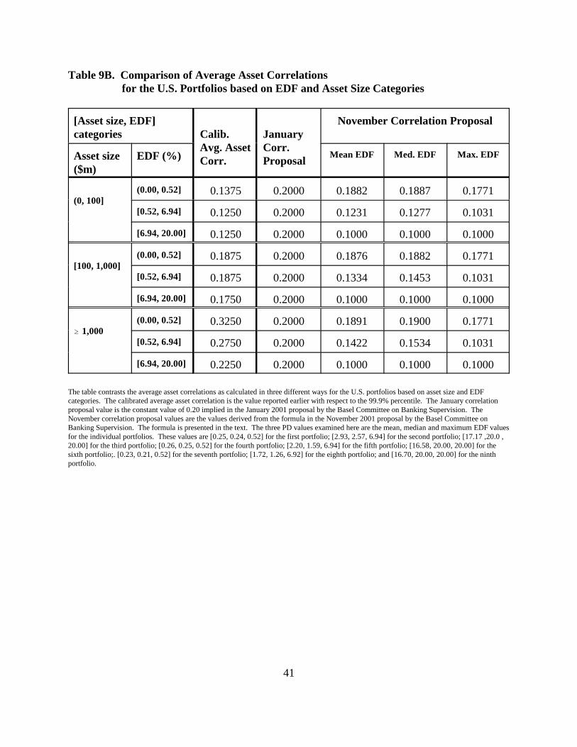
41

Table 9B. Comparison of Average Asset Correlations for the U.S. Portfolios based on EDF and Asset Size Categories


Avg. AssetCorr.



Asset size($m)


(0, 100](0.00, 0.52] 0.1375 0.2000 0.1882 0.1887 0.1771

[0.52, 6.94] 0.1250 0.2000 0.1231 0.1277 0.1031

[6.94, 20.00] 0.1250 0.2000 0.1000 0.1000 0.1000

[100, 1,000](0.00, 0.52] 0.1875 0.2000 0.1876 0.1882 0.1771

[0.52, 6.94] 0.1875 0.2000 0.1334 0.1453 0.1031

[6.94, 20.00] 0.1750 0.2000 0.1000 0.1000 0.1000

� 1,000(0.00, 0.52] 0.3250 0.2000 0.1891 0.1900 0.1771

[0.52, 6.94] 0.2750 0.2000 0.1422 0.1534 0.1031

[6.94, 20.00] 0.2250 0.2000 0.1000 0.1000 0.1000

The table contrasts the average asset correlations as calculated in three different ways for the U.S. portfolios based on asset size and EDFcategories. The calibrated average asset correlation is the value reported earlier with respect to the 99.9% percentile. The January correlationproposal value is the constant value of 0.20 implied in the January 2001 proposal by the Basel Committee on Banking Supervision. TheNovember correlation proposal values are the values derived from the formula in the November 2001 proposal by the Basel Committee onBanking Supervision. The formula is presented in the text. The three PD values examined here are the mean, median and maximum EDF valuesfor the individual portfolios. These values are [0.25, 0.24, 0.52] for the first portfolio; [2.93, 2.57, 6.94] for the second portfolio; [17.17 ,20.0 ,20.00] for the third portfolio; [0.26, 0.25, 0.52] for the fourth portfolio; [2.20, 1.59, 6.94] for the fifth portfolio; [16.58, 20.00, 20.00] for thesixth portfolio;. [0.23, 0.21, 0.52] for the seventh portfolio; [1.72, 1.26, 6.92] for the eighth portfolio; and [16.70, 20.00, 20.00] for the ninthportfolio.

42

Table 9C. Comparison of Average Asset Correlations for the Japanese Portfolios based on EDF and Asset Size Categories


Avg. AssetCorr.



Asset size($m)


(0, 200](0.00, 0.52] 0.2250 0.2000 0.1879 0.1878 0.1771

[0.52, 6.94] 0.2000 0.2000 0.1255 0.1317 0.1031

[6.94, 20.00] 0.2000 0.2000 0.1002 0.1003 0.1000

[200, 1,000](0.00, 0.52] 0.2250 0.2000 0.1892 0.1905 0.1771

[0.52, 6.94] 0.2500 0.2000 0.1282 0.1370 0.1032

[6.94, 20.00] 0.2750 0.2000 0.1002 0.1005 0.1000

� 1,000(0.00, 0.52] 0.4250 0.2000 0.1894 0.1903 0.1771

[0.52, 6.94] 0.4000 0.2000 0.1379 0.1477 0.1037

[6.94, 20.00] 0.5500 0.2000 0.1001 0.1002 0.1000

The table contrasts the average asset correlations as calculated in three different ways for the European portfolios based on asset size and EDFcategories. The calibrated average asset correlation is the value reported earlier with respect to the 99.9% percentile. The January correlationproposal value is the constant value of 0.20 implied in the January 2001 proposal by the Basel Committee on Banking Supervision. TheNovember correlation proposal values are the values derived from the formula in the November 2001 proposal by the Basel Committee onBanking Supervision. The formula is presented in the text. The three PD values examined here are the mean, median and maximum EDF valuesfor the individual portfolios. These values are [0.257, 0.260, 0.520] for the first portfolio; [2.735, 2.300, 6.940] for the second portfolio;[12.409, 11.450, 20.000] for the third portfolio; [0.228, 0.200, 0.520] for the fourth portfolio; [2.529, 1.990, 6.860] for the fifth portfolio;[12.566, 10.800, 20.000] for the sixth portfolio;. [0.224, 0.205, 0.520] for the seventh portfolio; [1.940, 1.480, 6.610] for the eighth portfolio;and [13.326, 12.420, 20.000] for the ninth portfolio.

43

Table 9D. Comparison of Average Asset Correlations for the European Portfolios based on EDF and Asset Size Categories


Avg. AssetCorr.



Asset size($m)


(0, 25](0.00, 0.52] 0.1250 0.2000 0.1895 0.1909 0.1771

[0.52, 6.94] 0.1250 0.2000 0.1253 0.1310 0.1031

[6.94, 20.00] 0.1250 0.2000 0.1001 0.1001 0.1000

[25, 200](0.00, 0.52] 0.1250 0.2000 0.1912 0.1932 0.1771

[0.52, 6.94] 0.1250 0.2000 0.1339 0.1438 0.1053

[6.94, 20.00] 0.1250 0.2000 0.1001 0.1001 0.1000

� 200(0.00, 0.52] 0.2000 0.2000 0.1919 0.1937 0.1771

[0.52, 6.94] 0.1750 0.2000 0.1422 0.1554 0.1032

[6.94, 20.00] 0.1750 0.2000 0.1001 0.1001 0.1000

The table contrasts the average asset correlations as calculated in three different ways for the Japanese portfolios based on asset size and EDFcategories. The calibrated average asset correlation is the value reported earlier with respect to the 99.9% percentile. The January correlationproposal value is the constant value of 0.20 implied in the January 2001 proposal by the Basel Committee on Banking Supervision. TheNovember correlation proposal values are the values derived from the formula in the November 2001 proposal by the Basel Committee onBanking Supervision. The formula is presented in the text. The three PD values examined here are the mean, median and maximum EDF valuesfor the individual portfolios. These values are [0.222, 0.190, 0.520] for the first portfolio; [2.748, 2.340, 6.930] for the second portfolio;[14.649, 15.040, 20.000] for the third portfolio; [0.185, 0.140, 0.520] for the fourth portfolio; [2.162, 1.650, 6.700] for the fifth portfolio;[14.450, 14.250, 20.000] for the sixth portfolio;. [0.170, 0.130, 0.520] for the seventh portfolio; [1.727, 1.180, 6.900] for the eighth portfolio;and [14.405, 15.03, 20.000] for the ninth portfolio.

44

Figure 1.

Calibrated Average Asset Correlations for the Aggregate Portfolios

0.0000

0.0500

0.1000

0.1500

0.2000

0.2500

0.3000

0.3500

0.4000

0.4500

All firms US firms JP firms EU firms

99.50% 99.90%

45

Figure 2A.

Calibrated Average Asset Correlations for World Portfolios based on EDF Categories

0.0000

0.0500

0.1000

0.1500

0.2000

0.2500

0.3000

0.3500

0.4000

0.4500

all EDF < 5 bp all EDF in(5,52] bp

all EDF in (52,203] bp

all EDF in(203,694] bp

all EDF in(694,2000] bp

99.50% 99.90%

46

Figure 2B.

Calibrated Average Asset Correlation for U.S. Portfolios based on EDF Categories

0.000

0.050

0.100

0.150

0.200

0.250

0.300

0.350

0.400

0.450

US EDF < 5 bp US EDF in(5,52] bp

US EDF in (52,203] bp

US EDF in(203,694] bp

US EDF in(694,2000] bp

99.50% 99.90%

47

Figure 2C.

Calibrated Average Asset Correlation for Japanese Portfolios Based on EDF Categories

0.000

0.050

0.100

0.150

0.200

0.250

0.300

0.350

0.400

0.450

JP EDF < 5 bp JP EDF in(5,52] bp

JP EDF in (52,203] bp

JP EDF in(203,694] bp

JP EDF in(694,2000] bp

99.50% 99.90%

48

Figure 2D.

Calibrated Average Asset Correlation for European Portfolios Based on EDF Categories

0.000

0.050

0.100

0.150

0.200

0.250

0.300

0.350

0.400

0.450

EU EDF < 5 bp EU EDF in(5,52] bp

EU EDF in (52,203] bp

EU EDF in(203,694] bp

EU EDF in(694,2000] bp

99.50% 99.90%

49

Figure 3A.

Calibrated Average Asset Correlations for World Portfolios based on Asset Size Categories

0.0000

0.0500

0.1000

0.1500

0.2000

0.2500

0.3000

0.3500

0.4000

0.4500

all < $20m all $(20, 100]m all $(100, 300]m all $(300, 1000]m all >$1000m

99.50% 99.90%

50

Figure 3B.

Calibrated Average Asset Correlation for U.S. Portfolios Based on Asset Size Categories

0.000

0.050

0.100

0.150

0.200

0.250

0.300

0.350

0.400

0.450

US <$20m US($20,$100]m

US($100,$300]m

US($300,$1000]m

US >$1000m

99.50% 99.90%

51

Figure 3C.

Calibrated Average Asset Correlations for Japanese Portfolios based on Asset Size Categories

0.000

0.050

0.100

0.150

0.200

0.250

0.300

0.350

0.400

0.450

JP <$100m JP($100,$200]m

JP($200,$400]m

JP($400,$1000]m

JP >$1000m

99.50% 99.90%

52

Figure 3D.

Calibrated Average Asset Correlations for European Portfolios based on Asset Size Categories

0.000

0.050

0.100

0.150

0.200

0.250

0.300

0.350

0.400

0.450

EU <$25massets

EU ($25,$75]massets

EU($75,$200]m

assets

EU($200,$1000]m

assets

EU >$1000massets

99.50% 99.90%

53

Figure 4A.

EDF < 52bpEDF [52, 694] bp

EDF > 694 bp

Size all <$75m

Size all $(100,500]m

Size all >$500m assets

0.0000

0.0500

0.1000

0.1500

0.2000

0.2500

0.3000

0.3500

0.4000

0.4500

Calibrated Average Asset Correlations at the 99.9% Percentile for World Portfolios based on Firm EDF and Asset Size Categories

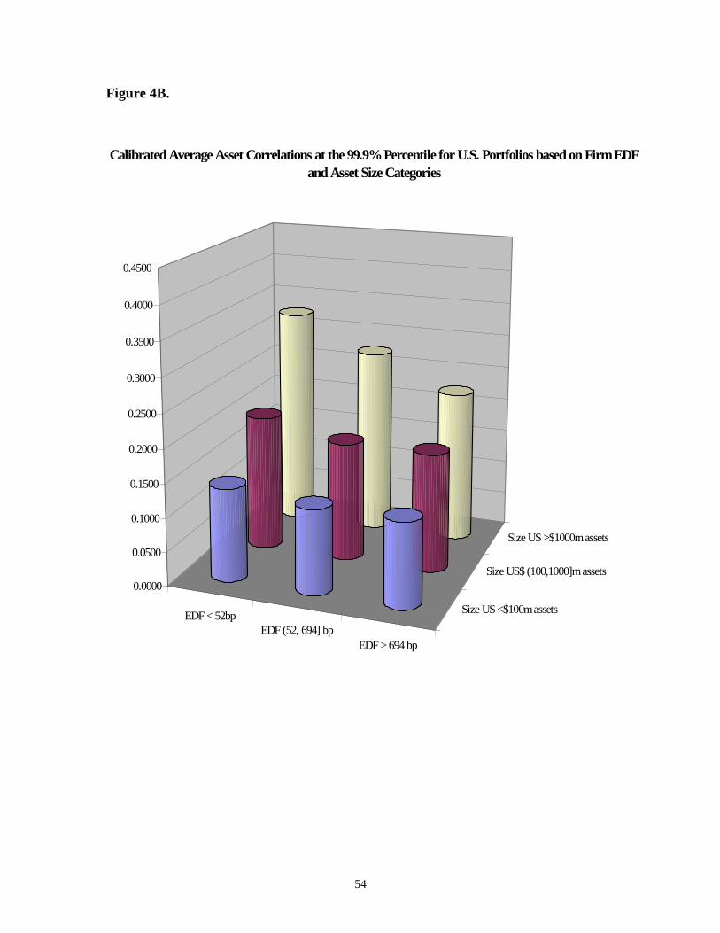
54

Figure 4B.

EDF < 52bpEDF (52, 694] bp

EDF > 694 bp

Size US <$100m assets

Size US$ (100,1000]m assets

Size US >$1000m assets

0.0000

0.0500

0.1000

0.1500

0.2000

0.2500

0.3000

0.3500

0.4000

0.4500

Calibrated Average Asset Correlations at the 99.9% Percentile for U.S. Portfolios based on Firm EDF and Asset Size Categories

55

Figure 4C.

Note that the calibrated average asset correlation for the Japanese portfolio based on the highest EDF andasset size categories is not plotted here in order to preserve the comparability of the other eight calibratedvalues. The average asset correlation for that portfolio was calibrated to be 0.5500.

EDF < 52bpEDF (52, 694] bp

EDF > 694 bp

JP <$200m assets

JP$ (200,1000]m assets

JP >$1000m assets

0.0000

0.0500

0.1000

0.1500

0.2000

0.2500

0.3000

0.3500

0.4000

0.4500

Calibrated Average Asset Correlations at the 99.9% Percentile for Japanese Portfolios based on Firm EDF and Asset Size Categories

56

Figure 4D.

EDF < 52bpEDF (52, 694] bp

EDF > 694 bp

EU <$25m assets

EU$ (25,200]m assets

EU >$200m assets

0.0000

0.0500

0.1000

0.1500

0.2000

0.2500

0.3000

0.3500

0.4000

0.4500

Calibrated Average Asset Correlations at the 99.9% Percentile for European Portfolios based on Firm EDF and Asset Size Categories

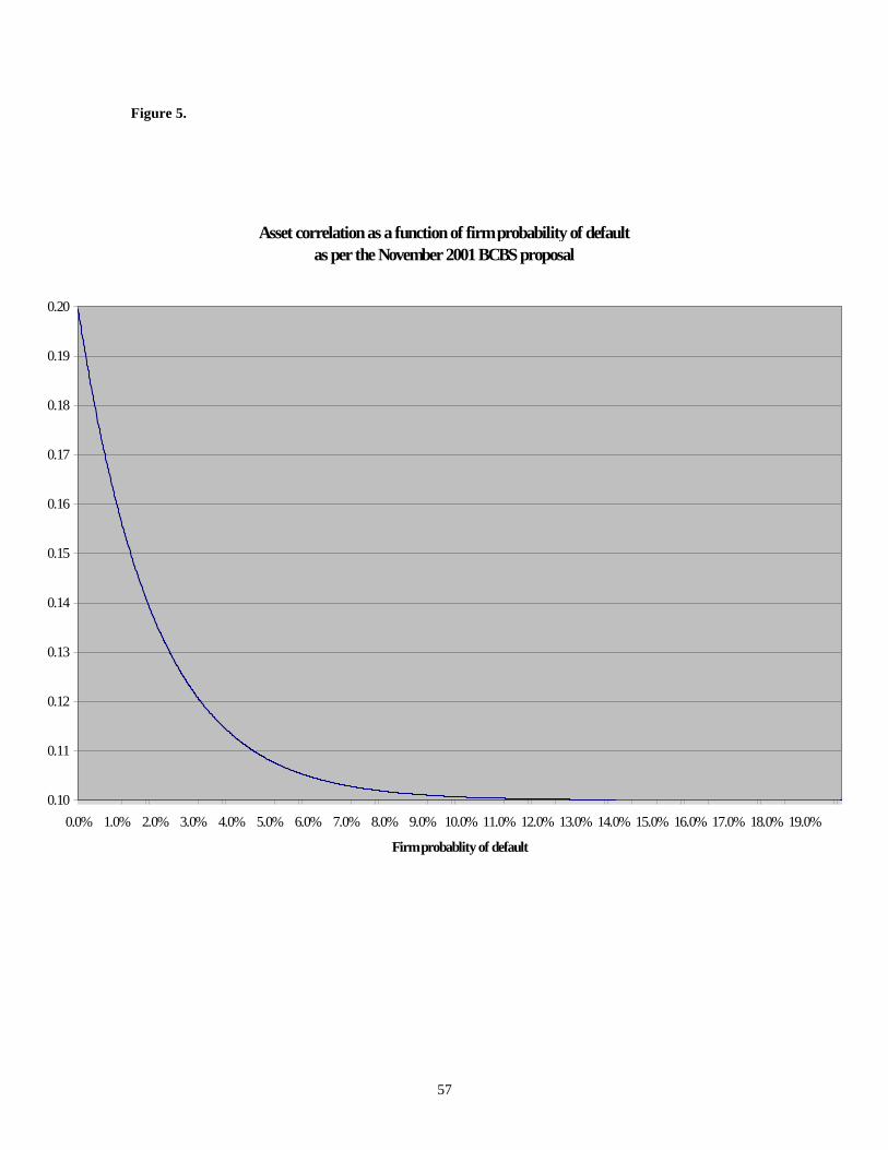
57

Figure 5.

Asset correlation as a function of firm probability of default as per the November 2001 BCBS proposal

0.10

0.11

0.12

0.13

0.14

0.15

0.16

0.17

0.18

0.19

0.20

0.0% 1.0% 2.0% 3.0% 4.0% 5.0% 6.0% 7.0% 8.0% 9.0% 10.0% 11.0% 12.0% 13.0% 14.0% 15.0% 16.0% 17.0% 18.0% 19.0%

Firm probablity of default

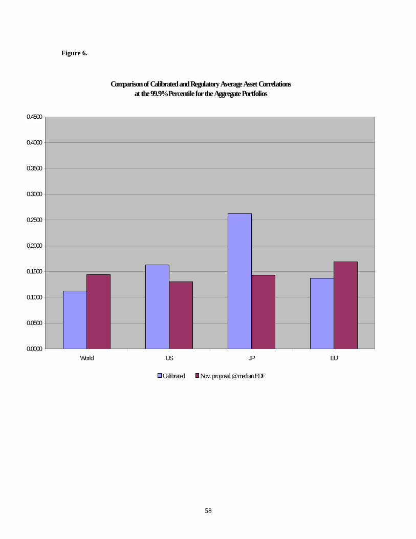
58

Figure 6.

Comparison of Calibrated and Regulatory Average Asset Correlationsat the 99.9% Percentile for the Aggregate Portfolios

0.0000

0.0500

0.1000

0.1500

0.2000

0.2500

0.3000

0.3500

0.4000

0.4500

World US JP EU

Calibrated Nov. proposal @ median EDF

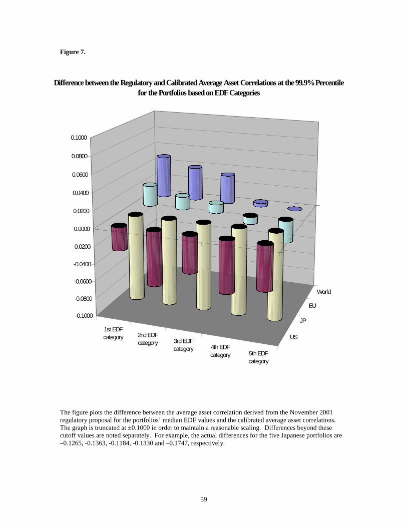
59

Figure 7.

The figure plots the difference between the average asset correlation derived from the November 2001regulatory proposal for the portfolios’ median EDF values and the calibrated average asset correlations.The graph is truncated at ±0.1000 in order to maintain a reasonable scaling. Differences beyond thesecutoff values are noted separately. For example, the actual differences for the five Japanese portfolios are–0.1265, -0.1363, -0.1184, -0.1330 and –0.1747, respectively.

1st EDFcategory 2nd EDF

category 3rd EDFcategory 4th EDF

category 5th EDFcategory

US

JP

EU

World

-0.1000

-0.0800

-0.0600

-0.0400

-0.0200

0.0000

0.0200

0.0400

0.0600

0.0800

0.1000

Difference between the Regulatory and Calibrated Average Asset Correlations at the 99.9% Percentile for the Portfolios based on EDF Categories

60

Figure 8.

The figure plots the difference between the average asset correlation derived from the November 2001regulatory proposal for the portfolios’ median EDF values and the calibrated average asset correlations.The graph is truncated at ±0.1000 in order to maintain a reasonable scaling. Differences beyond thesecutoff values are noted separately. For example, the actual differences for the last three Japanese portfoliosare –0.1130, -0.1583, and –0.2767, respectively.

1st sizecategory 2nd size

category 3rd sizecategory 4th size

category 5th sizecategory

US

JP

EU

World

-0.1000

-0.0800

-0.0600

-0.0400

-0.0200

0.0000

0.0200

0.0400

0.0600

0.0800

0.1000

Difference between the Regulatory and Calibrated Average Asset Correlations at the 99.9% Percentile for the Portfolios based on Asset Size Categories

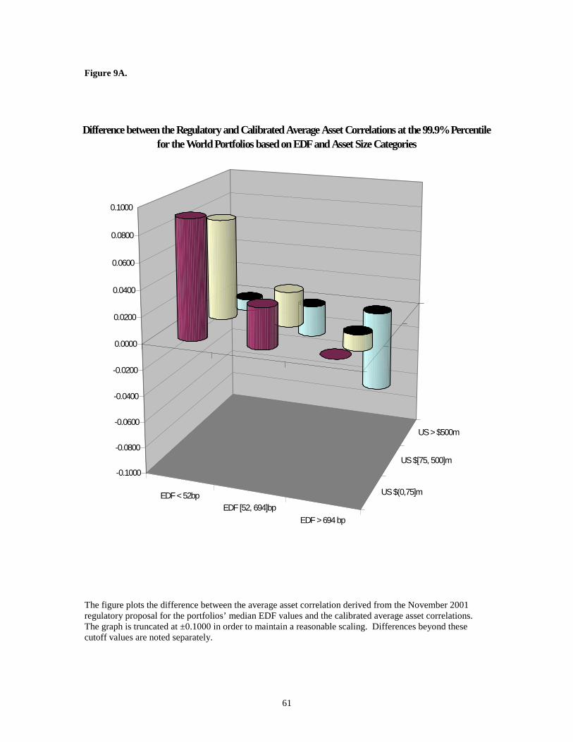
61

Figure 9A.

The figure plots the difference between the average asset correlation derived from the November 2001regulatory proposal for the portfolios’ median EDF values and the calibrated average asset correlations.The graph is truncated at ±0.1000 in order to maintain a reasonable scaling. Differences beyond thesecutoff values are noted separately.

EDF < 52bpEDF [52, 694]bp

EDF > 694 bp

US $(0,75]m

US $[75, 500]m

US > $500m

-0.1000

-0.0800

-0.0600

-0.0400

-0.0200

0.0000

0.0200

0.0400

0.0600

0.0800

0.1000

Difference between the Regulatory and Calibrated Average Asset Correlations at the 99.9% Percentile for the World Portfolios based on EDF and Asset Size Categories

62

Figure 9B.

The figure plots the difference between the average asset correlation derived from the November 2001regulatory proposal for the portfolios’ median EDF values and the calibrated average asset correlations.The graph is truncated at ±0.1000 in order to maintain a reasonable scaling. Differences beyond thesecutoff values are noted separately. For example, the actual differences for the three portfolios within thelargest size category are –0.1350, -0.1216, and –0.1250, respectively.


EDF > 694 bp

US $(0,100]m

US $[100, 1000]m

US > $1000m

-0.1000

-0.0800

-0.0600

-0.0400

-0.0200

0.0000

0.0200

0.0400

0.0600

0.0800

0.1000

Difference between the Regulatory and Calibrated Average Asset Correlations at the 99.9% Percentile for the US Portfolios based on EDF and Asset Size Categories

63

Figure 9C.

The figure plots the difference between the average asset correlation derived from the November 2001regulatory proposal for the portfolios’ median EDF values and the calibrated average asset correlations.The graph is truncated at ±0.1000 in order to maintain a reasonable scaling. Differences beyond thesecutoff values are noted separately. For example, the actual differences for the two largest EDF portfolioswithin the middle size category are –0.1130 and –0.1745, respectively. The actual differences for the threeEDF portfolios within the largest size category are –0.2347, -0.2523, and –0.4498, respectively


EDF > 694 bp

JP $(0,200]m

JP $[200, 1000]m

JP > $1000m

-0.1000

-0.0800

-0.0600

-0.0400

-0.0200

0.0000

0.0200

0.0400

0.0600

0.0800

0.1000

Difference between the Regulatory and Calibrated Average Asset Correlations at the 99.9% Percentile for the Japanese Portfolios based on EDF and Asset Size Categories

64

Figure 9D.

The figure plots the difference between the average asset correlation derived from the November 2001regulatory proposal for the portfolios’ median EDF values and the calibrated average asset correlations.The graph is truncated at ±0.1000 in order to maintain a reasonable scaling. Differences beyond thesecutoff values are noted separately


EDF > 694 bp

EU $(0,25]m

EU $[25, 200]m

EU > $200m

-0.1000

-0.0800

-0.0600

-0.0400

-0.0200

0.0000

0.0200

0.0400

0.0600

0.0800

0.1000

Difference between the Regulatory and Calibrated Average Asset Correlations at the 99.9% Percentile for the European Portfolios based on EDF and Asset Size Categories

Documents

The Empirical Relationship between Average Asset Correlation… · The Empirical Relationship between Average Asset Correlation, Firm Probability of Default and Asset Size Jose A