Embed Size (px)
Citation preview
The Environmental Fluid Dynamics Code Theory and Computation
Volume 1: Hydrodynamics and Mass Transport
Tetra Tech, Inc. 10306 Eaton Place
Suite 340 Fairfax, VA 22030
June 2007
EFDC Hydrodynamic and Transport Theory and Computation
2
Preface
This document comprises the first volume of the theoretical and computational
documentation for the Environmental Fluid Dynamics Code (EFDC). The material in
this volume was previously distributed as:
Hamrick, J. M., 1992: A THREE-DIMENSIONAL ENVIRONMENTAL FLUID
DYNAMICS COMPUTER CODE: THEORETICAL AND COMPUTATIONAL
ASPECTS. Special Report No. 317 in Applied Marine Science and Ocean Engineering,
Virginia Institute of Marine Science School of Marine Science, The College of William
and Mary, Gloucester Point, VA 23062
This original document is reproduced in its entirety with corrections to a number of errors
in equations listed at the end.
EFDC Hydrodynamic and Transport Theory and Computation
3
Acknowledgements
The Environmental Fluid Dynamics Code (EFDC) is a public domain, open source,
surface water modeling system, which includes hydrodynamic, sediment and
contaminant, and water quality modules fully integrated in a single source code
implementation. EFDC has been applied to over 100 water bodies including rivers, lakes,
reservoirs, wetlands, estuaries, and coastal ocean regions in support of environmental
assessment and management and regulatory requirements.
EFDC was originally developed at the Virginia Institute of Marine Science (VIMS) and
School of Marine Science of The College of William and Mary, by Dr. John M. Hamrick
beginning in 1988. This activity was supported by the Commonwealth of Virginia
through a special legislative research initiative. Dr. Robert Byrne, the late Dr. Bruce
Neilson, and Dr. Albert Kuo of VIMS are acknowledged for their efforts in supporting the
original development activity. Subsequent support for EFDC development at VIMS was
provided by the U.S. Environmental Protection Agency and the National Oceanic and
Atmospheric Administration’s Sea Grant Program. The contributions of VIMS staff and
former students including Mr. Gamble Sisson, Dr. Zaohqing Yang, Dr. Keyong Park, Dr.
Jian Shen, and Dr. Sarah Rennie are gratefully acknowledged.
Tetra Tech, Inc. (Tt) became the first commercial user of EFDC in the early 1990’s and
upon Dr. Hamrick’s joining Tetra Tech in 1996, the primary location for the continued
development of EFDC. Tetra Tech has provided considerable internal research and
development support for EFDC over the past 10 years and Mr. James Pagenkopf, Dr.
Mohamed Lahlou, and Dr. Leslie Shoemaker are gratefully acknowledged for this. Mr.
Michael Morton of Tetra Tech is particularly recognized for his many contributions to
EFDC development and applications. The efforts Tetra Tech colleagues including Dr.
Jeff Ji, Dr. Hugo Rodriguez, Mr. Steven Davie, Mr. Brain Watson, Dr. Ruiz Zou, Dr. Sen
Bai, Dr. Yuri Pils, Mr. Peter von Lowe, Mr. Will Anderson, and Dr. Silong Lu are also
recognized. Their wide-ranging applications of EFDC have contributed to the robustness
of the model and lead to many enhancements.
Primary external support of both EFDC development and maintenance and applications at
Tetra Tech over the past 10 years has been generously provided by the U.S.
Environmental Protection Agency including the Office of Science and Technology, the
Office of Research and Development and Regions 1 and 4. In particular, Dr. Earl Hayter
(ORD), Mr. James Greenfield (R4), Mr. Tim Wool (R4) and Ms. Susan Svirsky (R1) are
recognized for their contributions in managing both EFDC developmental and application
work assignments.
The ongoing evolution of the EFDC model has to a great extent been application driven
and it is appropriate to thank Tetra Tech’s many clients who have funded EFDC
applications over the past 10 years. The benefits of ongoing interaction with a diverse
group of EFDC users in the academic, governmental, and private sectors are also
acknowledged.
EFDC Hydrodynamic and Transport Theory and Computation
4
ABSTRACT
(Hamrick, 1992)
This report describes and documents the theoretical and computational aspects of a three-
dimensional computer code for environmental fluid flows. The code solves the three-
dimensional primitive variable vertically hydrostatic equations of motion for turbulent
flow in a coordinate system which is curvilinear and orthogonal in the horizontal plane
and stretched to follow bottom topography and free surface displacement in the vertical
direction which is aligned with the gravitational vector. A second moment turbulence
closure scheme relates turbulent viscosity and diffusivity to the turbulence intensity and a
turbulence length scale. Transport equations for the turbulence intensity and length scale
as well as transport equations for salinity, temperature, suspended sediment and a dye
tracer are also solved. An equation of state relates density to pressure, salinity,
temperature and suspended sediment concentration.
The computational scheme utilizes an external-internal mode splitting to solve the
horizontal momentum equations and the continuity equation on a staggered grid. The
external mode, associated with barotropic long wave motion, is solved using a semi-
implicit three time level scheme with a periodic two time level correction. A multi-color
successive over relaxation scheme is used to solve the resulting system of equations for
the free surface displacement. The internal mode, associated with vertical shear of the
horizontal velocity components is solved using a fractional step scheme combining an
implicit step for the vertical shear terms, with an explicit step for all other terms. The
transport equations for the turbulence intensity, turbulence length scale, salinity,
temperature, suspended sediment and dye tracer are also solved using a fractional step
scheme with implicit vertical diffusion and explicit advection and horizontal diffusion. A
number of alternate advection schemes are implemented in the code.
EFDC Hydrodynamic and Transport Theory and Computation
5
ACKNOWLEDGEMENT
(Hamrick, 1992)
The work described in this report was funded by the Commonwealth of Virginia under
the Three-Dimensional Model Research Initiative at the Virginia Institute of Marine
Science, College of William and Mary. Many members of the VIMS faculty and staff
provided advice, encouragement and support during the development of the
environmental fluid dynamics computer code described in this report. Dr. Albert Y. Kuo
is thanked for his continued technical advice and encouragement. The administrative
support of Drs. Robert J. Byrne and Bruce J. Neilson is gratefully acknowledged. Mr.
Gamble M. Sisson, Ms. Sarah Rennie, and Mr. John N. Posenau are thanked for their
support in data analysis, graphics programming and computer systems management.
EFDC Hydrodynamic and Transport Theory and Computation
6
CONTENTS
Preface
2
Acknowledgement
3
Abstract
4
Acknowledgement (Hamrick, 1992)
5
Contents
6
List of Figures
7
1. Introduction
8
2. Formulation of the Governing Equations
10
3. Numerical Solution Techniques for the Equations of
Motion
13
4. Computational Aspects of the External Mode Solution
17
5. Computational Aspects of the Internal Mode Solution
29
6. Numerical Solution Techniques for the Transport
Equations
34
7. The Environmental Fluid Dynamics Computer Code
44
8. Summary
46
9. References
48
10. Figures
51
Corrections 59
EFDC Hydrodynamic and Transport Theory and Computation
7
List of Figures
Figure 1. The stretched vertical coordinate system and the vertical
location of discrete variables.
51
Figure 2. Free surface displacement centered horizontal grid.
52
Figure 3. U centered grid in the horizontal (x,y) plane.
52
Figure 4. Dispersion relations: ωθ, vertical axis, versus kxmx and kymy,
horizontal axes, for wave propagation schemes.
53
Figure 5. Magnitude of phase velocity, |c|/sqrt(gh), vertical axis, as a
function of horizontal wave number, kxmx and kymy, horizontal axes.
54
Figure 6. Magnitude of group velocity, |G|/sqrt(gh), vertical axis, as a
function of horizontal wave number, kxmx and kymy, horizontal axes.
55
Figure 7. U centered grid in the vertical (x,z) plane.
56
Figure 8. S centered grid in the vertical (x,z) plane.
56
Figure 9. Dispersion relations: ωθ, vertical axis, versus kxmx and kymy,
horizontal axes, for advection schemes.
57
Figure 10. Magnitude of amplification factor, vertical axis, versus kxmx
and kymy, horizontal axes, for upwind advection scheme.
58
EFDC Hydrodynamic and Transport Theory and Computation
8
1. INTRODUCTION
The ability to predict the transport and mixing of materials discharged into the
hydrosphere and atmosphere is an essential element in environmental management. The
field of environmental fluid dynamics has emerged in response to the need to understand
and predict environmental fluid flows and the associated transport and mixing for
dissolved and suspended materials in these flows. A large range of space and time scales
characterize transport and mixing in the hydrologic and atmospheric environments. For
example, local mixing associated with the discharge of a buoyant waste fluid into an
ambient environmental flow can be described in terms of the three dimensional dynamics
of buoyant turbulent jets and plumes (Fischer et al., 1979). Outside of this region of local
or initial mixing, the further mixing and transport of discharged material is governed by
the dynamics of the ambient environmental flow.
A large class of incompressible ambient environmental flows is characterized by
horizontal length scales which are orders of magnitude greater than their vertical length
scales or length scales in the direction aligned with the gravitational vector. Such flows
are essentially hydrostatic in the vertical and of the boundary layer type. Example flows
in the hydrosphere range from rivers and lakes through estuaries and coastal seas to ocean
basins. Similarly in the atmosphere, mesoscale through global scale circulation can be
described by equations of motion simplified by the hydrostatic and boundary layer
approximations. This class of natural environmental flows is also characterized by
complex boundaries and topography and a host of nonlinear processes. The realistic
simulation of these complex flows necessitates the numerical solution of the equations of
motions and transport equations describing the transport and mixing of dissolved and
suspended materials.
The development of numerical or computational techniques appropriate for the solution
of the incompressible, vertically hydrostatic equations of motion occurred largely in the
field of numerical weather prediction. The monograph by Haltiner and Williams (1980)
and the volume edited by Chang (1977) provide excellent descriptions of the techniques
developed through the late 1970's. These techniques provided the basis for the
development of numerical ocean circulation models such as those of Bryan (1969) and
Semtner (1974). The growing concern for environmental problems in lakes, estuaries and
EFDC Hydrodynamic and Transport Theory and Computation
9
the coastal ocean lead to further development in numerical techniques and models
appropriate for these flow environments as typified by the work of Simons (1974), Liu
and Leendertse (1975), and Blumberg and Mellor (1987). Continuing developments in
estuarine and oceanic numerical modeling are presented in the recent volumes edited by
Heaps (1987) and Nihoul and Jamart (1987), while the text by Pielke (1984) presents
parallel developments in the modeling mesoscale atmospheric flows.
The purpose of the work presented herein is to formulate a numerical solution scheme for
incompressible, vertically hydrostatic environmental flows in the hydrosphere and
atmosphere, and to implement computationally that scheme in a computer code
appropriate for the range of computing platforms from personal to super computers. In
formulating the numerical solution scheme, the goal is not to reinvent the wheel, but to
build upon the large foundation of previous work briefly referenced in the preceding
paragraph, and extend it when appropriate to achieve improvements in accuracy, stability
and performance. The first version of the code and certain terminology in this report is
focused toward hydrospheric flows in estuaries and the coastal ocean, as well as lakes,
reservoirs and rivers. However, care has been taken to make the solution scheme and
code readily applicable to analeastic hydrostatic atmospheric flows by a simple
substitution of an appropriate equation of state. The remainder of the paper is organized
as follows. The governing equations of motion and transport equations are formulated in
Section 2. The overall numerical scheme for the equations of motion based on internal,
external mode splitting is presented in Section 3. Section 4 contains the formulation of
the numerical scheme for the external or long surface gravity wave mode and an analysis
of its stability and propagation characteristics. The internal, vertical shear or boundary
layer mode numerical scheme is presented in Section 5. The numerical schemes for the
transport equations are presented in Section 6. The computational aspects of the various
numerical schemes are also discussed in Sections 4, 5, and 6. Section 7 describes the
computational implementation of the numerical schemes in Environmental Fluid
Dynamics Computer Code (EFDC), and outlines a strategy for the code's application to
environmental fluid flow simulation and its complementary use as a research tool. Lastly,
Section 8 summarizes the important features of the numerical scheme and the
environmental fluid dynamics computer code.
EFDC Hydrodynamic and Transport Theory and Computation
10
2. FORMULATION OF THE GOVERNING EQUATIONS
The formulation of the governing equations for ambient environmental flows
characterized by horizontal length scales which are orders of magnitude greater than their
vertical length scales begins with the vertically hydrostatic, boundary layer form of the
turbulent equations of motion for an incompressible, variable density fluid. To
accommodate realistic horizontal boundaries, it is convenient to formulate the equations
such that the horizontal coordinates, x and y, are curvilinear and orthogonal. To provide
uniform resolution in the vertical direction, aligned with the gravitational vector and
bounded by bottom topography and a free surface permitting long wave motion, a time
variable mapping or stretching transformation is desirable. The mapping or stretching is
given by:
z= (z*
+ h) / (ζ + h) (1)
where * denotes the original physical vertical coordinates and -h and ζ are the physical
vertical coordinates of the bottom topography and the free surface respectively, Figure 1.
Details of the transformation may be found in Vinokur (1974), Blumberg and Mellor
(1987) or Hamrick (1986). Transforming the vertically hydrostatic boundary layer form
of the turbulent equations of motion and utilizing the Boussinesq approximation for
variable density results in the momentum and continuity equations and the transport
equations for salinity and temperature in the following form:
∂ t(mHu) + ∂x(myHuu) + ∂y (mxHvu) + ∂ z(mwu) − (mf + v∂x my −u∂y mx )Hv
= −my H∂x (gζ + p) − my(∂x h − z∂x H )∂ z p + ∂z(mH−1 Av∂ zu) + Qu
(2)
∂ t(mHv) + ∂x (myHuv) + ∂ y(mxHvv) + ∂z(mwv) + (mf + v∂x my − u∂y mx )Hu
= −mx H∂y (gζ + p) − mx(∂ yh − z∂y H )∂z p+ ∂z(mH−1Av∂z v) + Qv
(3)
∂z p = −gH(ρ − ρo)ρo
−1= −gHb
(4)
∂ t(mζ ) + ∂ x (myHu) + ∂ y(mx Hv) + ∂z(mw) = 0
(5)
∂ t(mζ ) + ∂ x (myH udz
0
1
∫ ) + ∂ y (mx H vdz0
1
∫ ) = 0
(6)
ρ = ρ( p,S,T) (7)
EFDC Hydrodynamic and Transport Theory and Computation
11
∂ t(mHS) + ∂ x(myHuS) + ∂ y (mx HvS) + ∂ z(mwS) = ∂ z(mH
−1Ab∂z S) + QS
(8)
∂ t(mHT) + ∂ x (myHuT) + ∂ y (mxHvT) + ∂z (mwT) = ∂ z(mH
−1Ab∂ zT) + QT
(9)
In these equations, u and v are the horizontal velocity components in the curvilinear,
orthogonal coordinates x and y, mx and my are the square roots of the diagonal
components of the metric tensor, m = mxmy is the Jacobian or square root of the metric
tensor determinant. The vertical velocity, with physical units, in the stretched,
dimensionless vertical coordinate z is w, and is related to the physical vertical velocity w*
by:
w = w
*− z(∂ tζ + umx
−1∂ xζ + vmy
−1∂ yζ ) + (1 − z)(umx
−1∂ xh+ vmy
−1∂ yh)
(10)
The total depth, H = h + ζ, is the sum of the depth below and the free surface
displacement relative to the undisturbed physical vertical coordinate origin, z* = 0. The
pressure p is the physical pressure in excess of the reference density hydrostatic pressure,
ροgH(1 - z), divided by the reference density, ρο. In the momentum equations (2, 3) f is
the Coriolis parameter, Av is the vertical turbulent or eddy viscosity, and Qu and Qv are
momentum source-sink terms which will be later modeled as subgrid scale horizontal
diffusion. The density, ρ, is in general a function of temperature, T, and salinity or water
vapor, S, in hydrospheric and atmospheric flows respectively and can be a weak function
of pressure, consistent with the incompressible continuity equation under the anelastic
approximation (Mellor, 1991; Clark and Hall, 1991). The buoyancy, b, is defined in
equation (4) as the normalized deviation of density from the reference value. The
continuity equation (5) has been integrated with respect to z over the interval (0,1) to
produce the depth integrated continuity equation (6) using the vertical boundary
conditions, w = 0, at z = (0,1), which follows from the kinematic conditions and equation
(10). In the transport equations for salinity and temperature, equations (8) and (9), the
source and sink terms, QS and QT include subgrid scale horizontal diffusion and thermal
sources and sinks, while Ab is the vertical turbulent diffusivity. It is noted that
constraining the free surface displacement to be time independent and spatially constant
yields the equivalent of the rigid lid ocean circulation equations employed by Smetner
(1974) and equations similar to the terrain following equations used by Clark (1977) to
model mesoscale atmospheric flow.
EFDC Hydrodynamic and Transport Theory and Computation
12
The system of eight equations (equations 2-9) provides a closed system for the variables
u, v, w, p, ζ, ρ, S, and T, provided that the vertical turbulent viscosity and diffusivity and
the source and sink terms are specified. To provide the vertical turbulent viscosity and
diffusivity, the second moment turbulence closure model developed by Mellor and
Yamada (1982) and modified by Galperin et al. (1988) will be used. The model relates
the vertical turbulent viscosity and diffusivity to the turbulent intensity, qq, a turbulent
length scale, l, and a Richardson number Rq by:
Av = φvql = 0.4(1 + 36Rq)
−1(1 + 6Rq)
−1(1 + 8Rq)ql
(11)
Ab = φbql = 0.5(1 + 36Rq)
−1ql
(12)
Rq =
gH∂zb
q2
l 2
H2
where the so-called stability functions φv and φb account for reduced and enhanced
vertical mixing or transport in stable and unstable vertically density stratified
environments, respectively. The turbulence intensity and the turbulence length scale are
determined by a pair of transport equations:
∂ t(mHq2) + ∂ x(myHuq
2) + ∂ y(mx Hvq
2) + ∂ z(mwq
2) = ∂z (mH
−1Aq∂ zq
2) + Qq
+2mH−1
Av (∂ zu)2
+ (∂ zv)2( )+ 2mgAb∂ zb − 2mH(B1l )
−1q
3
(13)
∂ t(mHq2l ) + ∂ x(myHuq
2l ) + ∂ y (mxHvq
2l ) + ∂ z(mwq
2l ) = ∂ z(mH
−1Aq∂z q
2l ) + Ql
+mH−1
E1l Av (∂z u)2
+ (∂z v)2( )+ mgE1E3l Ab∂ zb − mHB1
−1q
31 + E2 (κ L)
−2l
2( )
(14)
L
−1= H
−1z
−1+ (1 − z)
−1( )
(15)
where B1, E1, E2, and E3 are empirical constants and Qq and Ql are additional source-sink
term such as subgrid scale horizontal diffusion. The vertical diffusivity, Aq, is in general
taken equal to the vertical turbulent viscosity, Av.
EFDC Hydrodynamic and Transport Theory and Computation
13
3. NUMERICAL SOLUTION TECHNIQUES FOR THE EQUATIONS OF
MOTION
The equations of motion (equations 2-6) will be solved in a region subdivided into six
faced cells. The projection of the vertical cell boundaries to a horizontal plane forms a
curvilinear, orthogonal grid in the orthogonal coordinate system (x,y). In a vertical (x,z)
or (y,z) plane, the cells bounded by the same constant z surfaces will be referred to as cell
layers or layers. The equations will be solved using a combination of finite volume and
finite difference techniques, with the variable locations shown in Figure 2. The staggered
grid location of variables is often referred to as the C grid (Arakawa and Lamb, 1977) or
the MAC grid (Peyret and Taylor, 1983). To proceed, it is convenient to modify
equations (2,3) by eliminating the vertical pressure gradients using equation (4). After
some manipulation, the horizontal momentum equations become:
∂ t(mHu) + ∂x(myHuu) + ∂y (mxHvu) + ∂ z(mwu) − (mf + v∂x my −u∂y mx )Hv
= −my H∂x p − myHg∂ xζ + myHgb∂ xh − myHgbz∂ xH + ∂z(mH−1 Av∂ zu) + Qu
(16)
∂ t(mHv) + ∂x (myHuv) + ∂ y(mxHvv) + ∂z(mwv) + (mf + v∂x my − u∂y mx )Hu
= −mx H∂y p − mxHg∂ yζ + mxHgb∂yh − mx Hgbz∂yH + ∂z(mH−1 Av∂zv) + Qv
(17)
The vertical discretization of Equations (16,17) is considered first. The equations are
integrated with respect to z over a cell layer assuming that variables defined vertically at
the cell or layer centers are constant and that variables defined vertically at the cell layer
interfaces or boundaries vary linearly over the cell, to give:
∂ t(mH∆kuk) + ∂ x(myH∆kukuk ) + ∂ y(mxH∆kvkuk) + (mwu)k − (mwu)k−1
−(mf + vk∂ x my − uk∂ y mx)∆kHvk = − 0.5myH∆k∂ x( pk + pk−1) − myH∆k g∂xζ
+myH∆k gbk∂ xh− 0.5myH∆kgbk(zk + zk−1 )∂ xH + m(τ xz)k − m(τ xz)k−1 + (∆Qu)k
(18)
∂ t(mH∆kvk )k + ∂ x(my H∆kukvk ) + ∂ y (mx H∆kvkvk) + (mwv)k − (mwv)k−1
+(mf + vk∂ x my − uk∂ y mx)∆kHuk = − 0.5mx H∆k∂ y (pk + pk−1 ) − mx H∆kg∂ yζ
+mxH∆kgbk∂ yh− 0.5mx H∆kgbk (zk + zk−1 )∂ yH + m(τ yz )k − m(τ yz)k−1 + (∆Qv)k
(19)
where ∆k is the vertical cell or layer thickness, and the turbulent shear stresses at the cell
layer interfaces are defined by:
(τ xz)k = 2H−1
(Av)k(∆k+1 + ∆k )−1
(uk+1 − uk ) (20)
EFDC Hydrodynamic and Transport Theory and Computation
14
(τ yz )k = 2H
−1(Av)k(∆k+1 + ∆k )
−1(vk+1 − vk )
(21)
If there are K cells in the z direction, the hydrostatic equation can be integrated from a
cell layer interface to the surface to give:
pk = gH ∆ j bj − ∆kbkj = k
K
∑
+ ps
(22)
where ps is the physical pressure at the free surface or under the rigid lid divided by the
reference density. The continuity equation (5) is also integrated with respect to z over a
cell or layer to give:
∂ t(m∆kζ) + ∂x(my H∆kuk ) + ∂y (mxH∆kvk ) + m(wk − wk−1 ) = 0
(23)
The numerical solution of the vertically discrete momentum equations (18,19) now
proceeds by splitting the external depth integrated mode associated with external long
surface gravity waves from the internal mode associated with vertical current structure.
The external mode equations are obtained by summing equations (18,19) over K cells or
layers in the vertical utilizing equation (22), and are given by:
∂ t(mHu ) + ∂ x (myH∆kukuk ) + ∂ y (mxH∆kvkuk ) − H(mf + vk∂ x my − uk∂ ymx )∆kvk( )k=1
K
∑
= −my Hg∂xζ − my H∂ x ps + myHgb ∂xh− myHg ∆kβk + 0.5∆k (zk + zk −1)bk( )k=1
K
∑
∂ x H
−0.5myH2∂x ∆kβk
k=1
K
∑
+ m(τ xz)K − m(τxz)0 + Q u
(24)
∂ t(mHv ) + ∂ x (myH∆kukvk ) + ∂ y(mxH∆kvkvk ) + H(mf + vk∂x my − uk∂ y mx )∆kuk( )k=1
K
∑
= −mx Hg∂ yζ − mx H∂y ps + mxHgb ∂ yh− mxHg ∆kβk + 0.5∆k (zk + zk−1)bk( )k=1
K
∑
∂y H
−0.5mxH2∂ y ∆kβk
k=1
K
∑
+ m(τ yz)K − m(τ yz)0 + Q v
(25)
∂ t(mζ ) + ∂ x (myHu ) + ∂y (mx Hv ) = 0
(26)
EFDC Hydrodynamic and Transport Theory and Computation
15
βk = ∆ jbjj =k
K
∑ − 0.5∆kbk
(27)
where the over bar indicates an average over the depth. The depth integrated continuity
equation (26) follows from equation (6) and provides the continuity constraint for the
external mode. Consistent with the form of equation (26), the external mode variables
will be chosen to be the free surface displacement, ζ, and the volumetric transports myHu
and mxHv. Details of the solution of the external mode equations (24-26) are presented in
Section 4.
A number of formulations are possible for the internal mode equations. Equations
(18,19) have K degrees of freedom for each of the horizontal velocity components.
However, the summation of these equations over K cells or layers in the vertical to form
the external mode equations (24,25) effectively removes a degree of freedom since the
constraints:
∆k
k=1
K
∑ uk = u
(28)
∆k
k=1
K
∑ vk = v
(29)
must be satisfied. One approach to the internal mode is to solve equations (18,19) using
the free surface slopes, or the surface pressure gradients in the rigid lid case, from the
external solution and distribute the error such that equations (28,29) are satisfied. A
second approach is to form equations for the deviations of the velocity components from
their vertical means by subtracting the external equations (24,25) from the layer
integrated equations (18,19). However, it will still be necessary to satisfy the constraints
(28,29). The approach proposed herein is to reduce the systems of K layer averaged
equations (18,19) to systems of K-1 equations and use equations (28,29) to provide the
Kth equation consistent with the actual degrees of freedom.
The internal mode equations are formed by dividing equations (18,19) by the cell layer
thickness, ∆k, subtracting the equations for cell layer k from the equations for cell layer
k+1, and then dividing the results by the average thickness of the two cell layers to give:
∂ t mH∆k+1, k
−1(uk+1 − uk )( )+ ∂ x myH∆k+1, k
−1(uk+1uk +1 − ukuk)( )+ ∂ y mx H∆k+1,k
−1(vk+1uk+1 − vkuk )( )
EFDC Hydrodynamic and Transport Theory and Computation
16
+m∆k +1,k
−1∆k+1
−1(wu) k+1 − (wu)k( )− ∆k
−1(wu)k − (wu)k −1( )( )
− ∆k+1, k
−1(mf + vk+1∂x my − uk+1∂y mx )Hvk+1 − (mf + vk∂ x my − uk∂y mx )Hvk( )
= myH∆k+1, k−1 g(bk+1 − bk )(∂ xh − zk∂xH ) − 0.5myH
2∆k+1, k
−1 g(∆k+1∂xbk+1 + ∆k∂xbk )
+m∆k +1,k−1
∆k+1
−1 (τ xz) k+1 − (τ xz)k( )− ∆k−1 (τ xz)k − (τxz)k −1( )( )+ ∆k+1,k
−1 (Qu)k+1 − (Qu)k( )
(30)
∂ t mH∆k+1, k
−1(vk+1 − vk )( )+ ∂x myH∆k+1, k
−1(uk +1vk+1 − ukvk )( )+ ∂ y mxH∆k+1, k
−1(vk+1vk+1 − vkvk )( )
+m∆k +1,k−1
∆k+1
−1 (wv)k+1 − (wv)k( ) − ∆k−1 (wv)k − (wv)k−1( )( )
+ ∆k+1, k−1 (mf + vk+1∂x my − uk+1∂y mx )Huk+1 − (mf + vk∂ x my − uk∂y mx )Huk( )
= mxH∆k+1,k
−1g(bk+1 − bk )(∂ yh − zk∂yH) − 0.5mx H
2∆k+1, k
−1g(∆k+1∂ybk+1 + ∆k∂ybk )
+m∆k +1,k−1
∆k+1−1 (τ yz) k+1 − (τ yz)k( )− ∆k
−1 (τ yz)k − (τyz)k −1( )( )+ ∆k+1,k−1 (Qv )k+1 − (Qv) k( )
(31)
∆k +1,k = 0.5(∆k +1 + ∆k) (32)
Inspection of equations (30,31) reveals that they could have also been obtained by
differentiating the horizontal momentum equations (16,17) with respect to z and
introducing a finite difference discretion in z. Using equations (20,21) to relate the shear
stresses to the velocity differences across the interior interfaces suggest that equations
(30,31) be interpreted as a system of K-1 equations for either the K-1 interfacial velocity
differences or the K-1 interior interfacial shear stresses. Details of the solution of the
internal mode equations (30,31) will be presented in Section 5.
The solution of the vertical velocity, w, employs the continuity equations. Dividing
equation (23) by ∆k, and subtracting equation (26) gives:
wk = wk−1 − m
−1∆k ∂ x myH(uk − u )( )+ ∂ y mx H(vk − v )( )( )
(33)
Since wo = 0, the solution proceeds from the first cell layer to the surface. Provided the
constraints (equations 28-29) are satisfied, the surface velocity at k = K will be zero and
satisfy the boundary condition.
EFDC Hydrodynamic and Transport Theory and Computation
17
4. COMPUTATIONAL ASPECTS OF THE EXTERNAL MODE SOLUTION
The formulation of a computational algorithm for the numerical solution of the external
mode equations (24-26) begins by introducing modified variables and reorganizing the
equations to give:
∂ tU = −mx
−1myHg∂xζ − mx
−1myH∂x ps + mx
−1myHg b ∂xh − B ∂xH − 0.5H∂xβ ( )
−mx−1
∆k ∂x(Ukuk ) + ∂y (Vkuk )( )k=1
K
∑ + mx−1
∆k (mf + vk∂ x my − uk∂ymx )Hvk
k=1
K
∑
+my(τ xz)K − my (τ xz)0 + mx−1Q u
(34)
∂ tV = −mxmy
−1Hg∂yζ − mxmy
−1H∂ y ps + mxmy
−1Hg b ∂yh − B ∂y H − 0.5H∂yβ ( )
−my−1
∆k ∂x(Ukvk ) + ∂ y(Vkvk )( )k=1
K
∑ − my−1
∆k(mf + vk∂x my − uk∂y mx)Huk
k=1
K
∑
+mx(τ yz)K − mx (τ yz )0 + my−1Q v
(35)
∂ tζ + m
−1 ∂xU + ∂ yV ( ) = 0
(36)
U = myHu
(37)
V = mxHv (38)
Uk = myHuk (39)
Vk = mxHvk (40)
β = ∆kβk
k=1
K
∑
(41)
B = ∆kβ k + 0.5∆k (zk + zk−1 )bk( )
k =1
K
∑
(42)
Equations (34,35) now equate the time rate of change of the external or depth integrated
volumetric transports to the pressure gradients associated with the free surface slope,
atmospheric pressure and buoyancy, the advective accelerations, the Coriolis and
curvature accelerations, the free surface and bottom tangential stresses and the general
source, sink terms. The staggered location of variables on the computational grid, Figure
2, allows most horizontal spatial derivatives in equations (34-36) to be represented by
EFDC Hydrodynamic and Transport Theory and Computation
18
second order accurate central differences and results in conservation of volume, mass,
momentum and energy in the limit of exact integration of the equations in time (Simons,
1973; Haltiner and Williams, 1980). When a variable is not located at a point required
for implementation of central difference operators, averaging in either or both spatial
directions is appropriate. The use of the spatial averaging scheme of Arakawa and Lamb
(1977) to represent the Coriolis and curvature accelerations also guarantees energy
conservation.
Following the introduction of discrete finite difference and averaging representations in
space, equations (34-36), for a horizontal grid of L cells, may be viewed as a system of 3L
ordinary differential equations in time for the volumetric transport and the free surface
displacement. The numerous techniques available to solve these equations generally fall
within the two categories of explicit and semi-implicit. The most frequently used explicit
scheme is the three time level leapfrog scheme where the time derivatives are
approximated between time levels n+1 and n-1, and the remaining terms are evaluated at
time level n. Although computationally simple to implement, the maximum time step is
restricted by the Courant-Fredrick-Levy condition based on the gravity wave phase speed.
An alternate approach allowing larger time steps is the semi-implicit three time level
scheme (Madala and Piacsek, 1977), which when implemented for equations (34-36) is
U n+1
= U n−1
− θ(mx
−1my H)
ugδ x
u ζn+1+ ζ n −1( ) − 2θ (mx
−1myH )
uδ x
ups
+2θ(mx−1myH)u g b uδ x
uh − B uδ xuH − 0.5H uδ x
uβ ( )− 2θ (mx−1 )u
∆k δ xu(Ukuk ) + δ y
u(Vkuk )( )k=1
K
∑
+2θ(mx
−1)
u∆k (mf + vk∂ x my − uk∂ y mx )Hvk( )
u
k=1
K
∑ + 2θ my
u(τ xz
n −1)K − (τxz
n−1)0( )
u
+2θ(mx
−1)
u∆k ∂ x myHτ xx
n−1( )+ ∂ y mxHτ xy
n −1( )+ ∂ ymxHτ xy
n −1− ∂ xmyHτ yy
n−1( )k
u
k=1
K
∑
(43)
V n+1
= V n−1
− θ(mxmy
−1H)
vgδ y
v ζ n+1+ ζn−1( )− 2θ(mxmy
−1H )
vδ y
vps
+2θ(mxmy−1H )v g b vδ y
vh− B vδ yvH − 0.5H vδ y
vβ ( )− 2θ(my−1)v
∆k δ xv (Ukvk ) +δ y
v (Vkvk )( )k=1
K
∑
−2θ(my
−1)
v∆k (mf + vk∂ x my − uk∂ y mx )Huk( )
v
k=1
K
∑ + 2θ mx
v(τyz
n−1)K − (τ yz
n−1)0( )
v
+2θ(my
−1)
v∆k ∂ x myHτ yx
n−1( )+ ∂y mx Hτyy
n−1( )− ∂ ymxHτ xx
n−1+ ∂ xmyHτyx
n −1( )k
v
k=1
K
∑
(44)
ζn +1
− ζ n−1+ θ (m
−1)
ζ δx
ζ(U
n+1+U
n −1) +δy
ζ(V
n+1+ V
n −1)( )= 0
(45)
EFDC Hydrodynamic and Transport Theory and Computation
19
with θ being the time step. All terms in equations (43-45) are understood to be evaluated
at the center time level n except those evaluated at the forward and backward time levels,
n+1 and n-1, which are denoted by superscripts. The u, v, and ζ superscripts indicate that
a variable is evaluated, or that a spatial derivative is centered, at the corresponding spatial
point.
The subscript of the spatial central difference operator, δ, indicates direction. The grid
cells are presumed to be bounded in the horizontal by lines of constant integer values of
the dimensionless orthogonal coordinates x and y, resulting in the central spatial
differences having the forms:
δx φ(x, y)( ) = φ(x + 0.5,y) − φ (x − 0.5, y) (46)
δy φ(x,y)( ) = φ(x, y + 0.5) − φ (x, y − 0.5)
(47)
Application of these finite difference operators to the advective accelerations is illustrated
by:
δx
uUk(x)uk (x)( ) = Uk(x + 0.5)uk (x + 0.5) −Uk (x − 0.5)uk(x − 0.5)
(48)
where the constant y dependence of the variables is implied. Since the u type variables
are located at integer values of x, averaging is necessary to obtain values at the half
intervals. Averaging both the transport and the velocity gives:
δx
uUk(x)uk (x)( ) = 0.25 Uk (x +1) +Uk (x)( ) uk(x +1) + uk (x)( )
−0.25 Uk(x) +Uk (x −1)( ) uk (x) + uk (x −1)( )
(49)
which is consistent with a central difference approximation of the non-conservative form
of this portion of the advective acceleration. Averaging the transport and allowing the
velocity to be advected from the upwind direction gives:
δx
uUk(x)uk (x)( ) = 0.5Max Uk(x +1) + Uk(x)( ),0( )uk
n−1(x, y)
+0.5Min Uk (x +1) +Uk (x)( ),0( )ukn−1(x +1, y)
−0.5Max Uk (x) + Uk(x −1)( ),0( )uk
n −1(x −1, y)
−0.5Min Uk (x) +Uk (x −1)( ),0( )ukn−1(x, y)
(50)
EFDC Hydrodynamic and Transport Theory and Computation
20
which is consistent with an upwind or backward difference approximation of the non-
conservative form of this portion of the advective acceleration. In equation (50), the
transport is still at time level n, while the velocity is at time level n-1, for both stability
and accuracy (Smolarkiewicz and Clark, 1986). The preference for the use of equation
(49) or equation (50) will generally depend upon the physical situation being simulated.
The central difference form introduces no numerical diffusion but may produce solution
fields which exhibit cell to cell spatial oscillations. These oscillations can be eliminated
by the addition of horizontal diffusion terms to the momentum equations. Specification
of the horizontal diffusivity allows the degree of spatial smoothing to be controlled. The
upwind difference form introduces numerical diffusion and does not produce spatial
oscillations in the solution field. The Coriolis and curvature terms in equations (43,44)
are discretized using an energy conserving spatial averaging and differencing (Arakawa
and Lamb, 1977; Haltiner and Williams, 1980). For example, the Coriolis and curvature
term in equation (43) is given by:
(mf + vk∂ x my − uk∂ymx )Hvk( )
u
= 0.5 RHvk( )ζ
(x + 0.5, y) + RHvk( )ζ(x − 0.5,y)( )
(51)
Rkζ (x + 0.5) = fm(x + 0.5, y) + vk
ζ (x + 0.5, y) my(x + 1,y) − my (x, y)( )−uk
ζ (x + 0.5,y) mx (x + 0.5, y + 0.5) − mx (x + 0.5, y − 0.5)( )
(52)
vk
ζ(x + 0.5, y) = 0.5 vk(x + 0.5, y + 0.5) + vk (x + 0.5, y − 0.5)( )
(53)
uk
ζ(x + 0.5, y) = 0.5 uk (x +1, y) + uk (x, y)( )
(54)
where the variables locations are shown in Figure 3.
Since the bottom tangential stresses in equations (43,44) must be supplied from the
internal mode solution which follows the external solution, it is lagged at the backward
time level. The general source, sink term has been replaced by horizontal diffusion terms
having the form proposed by Mellor and Blumberg (1985). The horizontal stress tensor is
taken of the form:
τ xx( )
k= 2AHmx
−1∂xuk (55)
τ xy( )
k= τ yx( )
k= 2AH mx
−1∂xvk + my
−1∂yuk( )
(56)
τ yy( )
k= 2 AHmy
−1∂yvk (57)
EFDC Hydrodynamic and Transport Theory and Computation
21
The horizontal diffusion coefficient, AH, is often specified as a minimum constant value
necessary to smooth cell to cell spatial oscillations in the solution field when the central
difference form of the advective acceleration, equation (49) is used. When the horizontal
turbulent diffusion is used to represent subgrid scale mixing, AH may be determined as
suggested by Smagorinsky (1963).
The solution scheme for equations (43-45) involves first evaluating all terms in the three
equations at time levels n and n-1. On boundaries where the transports are specified, the
specified values at time level n+1 are inserted into equation (45). Equations (43,44) are
then used to eliminate the unknown transports at time level n+1, from equation (45). The
result is a discrete Helmholtz type elliptic equation for the free surface displacement at
time level n+1, having the general form:
ζn +1
− gθ2(m
−1)
ζ δ x
ζ(mx
−1my H)
uδ x
uζ n+1( )+ δ y
ζ(mxmy
−1H )
vδ y
vζ n+1( )( )− φ = 0
(58)
with the term φ containing all of the previously evaluated terms and transport boundary
conditions. For cells where the free surface displacement is specified, equation (58) is
replaced by an equation which enforces the specified boundary condition at time level
n+1. For the rigid lid case where the free surface displacement is constant in time and
space, equation (58) is modified to give an equation for the unknown surface pressure, ps,
by eliminating the first term, replacing gζ in the discrete elliptic operator by ps, and
appropriately modifying the last term. In the computer code, the system of equations
corresponding to equation (58) is solved by a reduced system conjugate gradient scheme
with a multicolor or red-black ordering of the cells (Hageman and Young, 1981). The
conjugate gradient iterations continue until the sum of the squared residuals is less than a
specified value. The free surface displacements or surface pressures are then substituted
into equations (43,44) to determine the transports at time level n+1. Since the solution of
equation (58) is approximate, equation (45) may not be identically satisfied upon
substitution of the time level n+1 transports and free surface displacement. To insure that
equation (45) is identically satisfied in the case of a dynamic free surface, it is solved for
a revised value of the time level n+1, free surface displacement after introduction of the
time level n+1 transports. For the rigid lid case, an external divergence error is calculated
and compensated for by adding appropriate volumetric source or sink terms to equation
(45) during the next time step.
EFDC Hydrodynamic and Transport Theory and Computation
22
Some insight into the stability and accuracy of the semi-implicit three time level scheme
for solving the external mode equations with a dynamically active free surface can be
gained by a Fourier analysis of the linearized discrete equations:
U
n+1= U
n−1− θ(mx
−1myho)
ugδ x
u ζn +1+ ζ n−1( )+ 2θ(mx
−1my )
uf V
u
(59)
V
n+1= V
n−1− θ(mxmy
−1ho)
vgδ y
v ζn+1+ ζ n −1( )− 2θ (mxmy
−1)
vf U
v
(60)
ζn +1
− ζ n−1+ θ (m
−1)
ζ δx
ζ(U
n+1+U
n −1) +δy
ζ(V
n+1+ V
n −1)( )= 0
(61)
Introduction of the Fourier representations:
U
V
W
=
Uo
Vo
Wo
exp iω nθ + ikxmxx + ikymyy( )
(62)
W = ghom ζ
(63)
on a rectangular Cartesian grid gives the eigenvalue problem:
λ2
M+ + λ M + M− = 0 (64)
M+ =
1 0 2imx
−1myCsin 0.5kxmx( )
0 1 2imxmy
−1Csin 0.5kymy( )
2iC sin 0.5kxmx( ) 2iC sin 0.5kymy( ) 1
(65)
M = 2 fθ cos 0.5kxmx( )cos 0.5kymy( )0 −mx
−1my 0
mxmy
−10 0
0 0 0
(66)
M− =
−1 0 2imx
−1myCsin 0.5kxmx( )
0 −1 2imxmy
−1Csin 0.5kymy( )
2iC sin 0.5kxmx( ) 2iC sin 0.5kymy( ) −1
(67)
C =
gho
mθ
(68)
EFDC Hydrodynamic and Transport Theory and Computation
23
where ω is the frequency, kx and ky are the wave numbers and C is the Courant number
associated with the shallow water wave speed.
The eigenvalue, λ, is related to the frequency and time step by:
λ = λ exp(iω θ) (69)
The characteristic polynomial of equation (64) is:
λ2
− 1( ) λ4− 2ψλ2
+1( )= 0
(70)
ψ =
1− 4C2 my
mx
sin2 kxmx
2
+
mx
my
sin2 kymy
2
− 2 f
2θ 2cos
2 kxmx
2
cos
2 kymy
2
1+ 4C2 my
mx
sin2 kxmx
2
+
mx
my
sin2 kymy
2
(71)
and the roots or eigenvalues are:
λ = 1, ψ + i 1 − ψ 2
, ψ − i 1 − ψ 2,−1,− ψ + i 1 − ψ 2
,− ψ − i 1 − ψ 2
(72)
For linear stability, the absolute values of the eigenvalues must be less than or equal to
one. The absolute values of the four complex eigenvalues are identically one, provided
the absolute value of ψ is less than one, which requires:
θ ≤ f−1
(73)
Thus the linearized three time level semi-implicit scheme is neutrally stable when
equation (73) is satisfied. Since at mid-latitude the inverse of the Coriolis parameter is on
the order of 10,000 sec, the time step is not overly constrained. The overall stability of
the scheme will most likely be controlled by the stability of the explicit advective and
curvature accelerations. The form of the curvature terms in the momentum equations
suggest that they may increase the effective magnitude of the Coriolis parameter and
reduce the stable time step. The stability of the explicit scheme for the advective
accelerations will be discussed in subsequent sections.
The major computational problem with three time level schemes for systems of first order
equations is the doubling of the number of eigenvalues over those physically
EFDC Hydrodynamic and Transport Theory and Computation
24
characterizing the system. The eigenvalues in equation (72) are grouped such that the
first three correspond to the true physical solution or physical mode of the system while
the last three are spurious and give rise to what is referred to as the computational mode
(Haltiner and Williams, 1980). Expressing the physical mode eigenvalues of the
numerical scheme in terms of ωθ, using equation (69), gives the dispersion relation:
ωθ = 0, ±0.5arccos ψ( )
(74)
which can be compared with the dispersion relation
ωθ = 0, ± f
2θ2+ mx
−1my Ckxmx( )
2
+ mxmy
−1Ckymy( )
2
(75)
for the continuous in time and space form of equations (59-61). Both the numerical and
continuous solutions are characterized by a steady mode and pairs of waves propagating
in opposite directions. The major feature of the computational mode of the numerical
solution scheme, represented by the last three eigenvalues in equation (72), is an
alternating change in sign of the solution at every time step. Since all eigenvalues of the
scheme are neutrally stable, the computational mode solution can persist and become a
source of error. Two alternatives to eliminating the computational mode are the
application of weak time filter or the periodic insertion of a single step using a two time
level scheme (Haltiner and Williams, 1980). For the present work, the insertion of a two
time level step or possibly more appropriately termed a correction step was selected.
The correction step used to eliminate the computational mode is a trapezoidal scheme.
The scheme computes a corrected time level n+1 solution using the initial condition at
time level n and the solution at time level n+1 previously computed using the three time
level scheme. The momentum and continuity equations, equivalent to equations (43-45),
for the trapezoidal correction step are:
U n+1 = U n − 0.5θ(mx−1my H
n +1
2 )u gδxu ζn +1+ ζ n( )− θ (mx
−1myH )uδxups( )
n+ 1
2
+θ (mx−1myH )ug b uδ x
uh − B uδxuH − 0.5H uδx
uβ ( )( )n+
1
2
− θ (mx−1 )u
∆k δ xu(Ukuk ) + δ y
u(Vkuk )( )k=1
K
∑
+θ (mx
−1)
u∆k (mf + vk∂x my − uk∂ ymx )Hvk( )
u( )n+
1
2
k=1
K
∑ + θ my
u(τ xz
n)K − (τ xz
n)0( )
u
+θ (mx
−1)
u∆k ∂x myHτ xx
n( )+ ∂ y mxHτ xy
n( )+ ∂ymx Hτ xy
n− ∂xmyHτ yy
n( )k
u
k=1
K
∑
(76)
EFDC Hydrodynamic and Transport Theory and Computation
25
V n+1 = V n − 0.5θ(mxmy−1H
n+1
2 )v gδ yv ζn+1 + ζn( )− θ (mxmy
−1H )vδ yv ps( )
n+ 1
2
+θ (mxmy−1H )v g b vδ y
vh− B vδ yvH − 0.5H vδ y
vβ ( )( )n+
1
2
− θ(my−1) v
∆k δ xv (Ukvk ) + δ y
v (Vkvk )( )k=1
K
∑
−θ (my
−1)
v∆k (mf + vk∂x my − uk∂ y mx )Huk( )
v( )n+
1
2
k =1
K
∑ + θ mx
v(τ yz
n)K − (τyz
n)0( )
v
+θ (my
−1)
v∆k ∂ x myHτ yx
n( )+ ∂ y mx Hτ yy
n( )− ∂ ymxHτ xx
n+ ∂ xmyHτ yx
n( )k
v
k=1
K
∑
(77)
ζn +1
− ζ n+ 0.5θ (m
−1)
ζ δ x
ζ(U
n+1+U
n) +δ y
ζ(V
n+1+ V
n)( )= 0
(78)
where the notation n+1/2 implies:
( )
n +1
2 = 0.5 ( )*
+ ( )n( )
with * denoting evaluation using time level n+1 results from the previous three time level
step. Because of stability restrictions, the advective accelerations must be of the upwind
form:
δxu Uk(x)uk (x)( ) = 0.5Max Uk(x +1) + Uk(x)( ),0( )
n+1
2 ukn(x, y)
+0.5Min Uk (x +1) +Uk (x)( ),0( )n+
1
2 ukn(x +1, y)
−0.5Max Uk (x) + Uk(x −1)( ),0( )n+ 1
2 uk
n(x −1,y)
−0.5Min Uk (x) +Uk (x −1)( ),0( )n+
1
2 ukn(x, y)
( 79)
The solution of semi-implicit equations (76-78) follows that outlined for the three time
level scheme.
To analyze the stability of the trapezoidal correction step with a dynamically active free
surface, two points of view will be considered. Since a single application of the
trapezoidal scheme essentially corrects a step of the three time level scheme, it is actually
three time level. The Fourier analysis of the combined linearized three time level,
trapezoidal correction scheme on a rectangular Cartesian grid gives the eigenvalue
problem:
λ2
N + + λ (N + N − − NM+
−1M) − NM+
−1M− = 0 ( 80)
EFDC Hydrodynamic and Transport Theory and Computation
26
N + =
1 0 imx
−1myCsin 0.5kxmx( )
0 1 imxmy
−1C sin 0.5kymy( )
iC sin 0.5kxmx( ) iC sin 0.5kymy( ) 1
(81 )
N = 0.5 fθ cos 0.5kxmx( )cos 0.5kymy( )0 −mx
−1my 0
mxmy
−10 0
0 0 0
(82 )
N − =
−1 0 imx
−1myCsin 0.5kxmx( )
0 −1 imxmy
−1C sin 0.5kymy( )
iC sin 0.5kxmx( ) iC sin 0.5kymy( ) −1
(83 )
The sixth order characteristic polynomial of equation (80) is algebraically rather complex
and only the two roots or eigenvalues, 1 and 0, can be determined in closed form. The
eigenvalue of one is associated with the steady physical mode, while the eigenvalue of
zero is spurious but serves a useful purpose in eliminating the computational mode. A
second point of view is that the successive application of the trapezoidal correction is
equivalent to an iterative two time level scheme. The Fourier analysis of such a scheme
gives the eigenvalue problem:
λ (N+ + N) + (N + N− ) = 0 ( 84)
whose characteristic polynomial is:
λ −1( ) λ2
− 2χλ +1( )= 0
(85 )
where
χ =
1 − C2 my
mx
sin2 kxmx
2
+
mx
my
sin2 kymy
2
−
1
4f
2θ 2cos
2 kxmx
2
cos
2 kymy
2
1 + C2 my
mx
sin2 kxmx
2
+
mx
my
sin2 kymy
2
+
1
4f 2θ 2 cos2 kxmx
2
cos2 kymy
2
(86 )
The roots or eigenvalues of equation (80) are:
λ = 1,χ + i 1 − χ 2, χ − i 1 − χ 2
(87 )
EFDC Hydrodynamic and Transport Theory and Computation
27
Since the absolute value of χ is always less than one, the absolute value of the complex
eigenvalues is identically one and the scheme is neutrally and unconditionally stable.
The results of the Fourier analysis is also useful in accessing the accuracy of the external
mode solution scheme with respect to its ability to represent the dispersion relation and
the phase and group velocities of shallow water waves (Foreman, 1983). The dispersion
relations for the continuous in space and time shallow water equations, and the three and
two time level schemes, respectively, are:
ωθ = f
2θ 2+ mx
−1my Ckxmx( )
2+ mxmy
−1Ckymy( )
2
(88 )
ωθ = 0.5arccos(ψ ) ( 89)
ωθ = arccos(χ ) (90 )
where ψ and χ are given by equations (71,86). The phase and group velocities are given
respectively by:
(cx,cy)
gho
=(kx ,ky)
m kx2 + ky
2( )ωθ
C
(91 )
Gx,Gy( )gho
=1
m
∂
∂kx
,∂
∂ ky
ωθ
C
( 92)
A comparison of the dispersion relations for a square Cartesian grid with a Courant
number of 5 and f θ of 0.01 is shown in Figure 4. The dispersion relations for the three
time level and the two time level, included for comparison, difference schemes show
excellent agreement with the continuous equations for dimensionless wave numbers less
than approximately 0.05. As the dimensionless wave number magnitude increases toward
0.1, both numerical schemes under predict the dimensionless frequency with the three
time level scheme being less accurate than the two time level scheme. The magnitudes of
the phase velocity as a function of the dimensionless horizontal wave numbers are shown
in Figure 5. Both numerical schemes increasingly under predict the phase velocity
magnitude as the wave number magnitude increases, but provide relatively accurate
predictions for dimensionless magnitudes less than 0.05, with the two time level scheme
being more accurate. The magnitudes of the group velocity as a function of the
dimensionless horizontal wave numbers are shown in Figure 6. Again the numerical
EFDC Hydrodynamic and Transport Theory and Computation
28
schemes increasingly under predict the group velocity magnitude as the wave number
magnitude increases, but provide relatively accurate predictions for dimensionless
magnitudes less than 0.05. Although the two time level scheme is shown to be more
accurate than the three time level scheme at higher wave number magnitudes, it would be
computationally much more costly to implement due to the iterative evaluation of the
Coriolis, curvature and advective accelerations.
EFDC Hydrodynamic and Transport Theory and Computation
29
5. COMPUTATIONAL ASPECTS OF THE INTERNAL MODE SOLUTION
The internal mode equations (30,31) are solved using a fractional step scheme (Peyret and
Taylor, 1983), with the first step being explicit and the second step being implicit. Figure
7 illustrates the location variables in the x,z plane for the x componoent of the internal
mode equations. The computational equations for the three time level explicit step are:
Uk +1 − Uk( )**
= Uk+1 −Uk( )n−1
− 2θ (mx−1 )u δ x
u(Uk +1uk+1 − Ukuk ) +δ yu(Vk+1uk+1 − Vkuk )( )
−2θ(mx
−1)
u∆k+1
−1(Wu)k+1 − (Wu)k( )− ∆k
−1(Wu)k − (Wu)k−1( )( )
u
+2θ(mx−1 )u (mf + vk+1∂x my − uk+1∂ y mx )Hvk +1 − (mf + vk∂x my − uk∂ymx )Hvk( )
u
+2θ(mx−1myH)u g (bk+1 − bk )uδ x
u(h− zk H) − 0.5H uδxu(∆k+1bk +1 + ∆kbk )( )
+2θ(mx−1 )u (Qu)k+1 − (Qu)k( )
u
(94)
Vk+1 − Vk( )**
= Vk+1 − Vk( )n−1
− 2θ(my
−1)
v δ x
v(Uk +1vk+1 − Ukvk ) + δ y
v(Vk+1vk+1 − Vkvk )( )
−2θ(my−1)v
∆k+1
−1 (Wv)k+1 − (Wv)k( ) − ∆k−1 (Wv)k − (Wv)k−1( )( )
v
−2θ(my−1)v (mf + vk+1∂ x my − uk+1∂ y mx )Huk+1 − (mf + vk∂ x my − uk∂ y mx)Huk( )
v
+2θ(mxmy−1H )v g (bk+1 − bk )v δ y
v (h − zkH ) − 0.5H vδ yv (∆k+1bk +1 + ∆kbk )( )
+2θ(my−1 )v (Qv )k+1 − (Qv)k( )
v
(95 )
W = mw= mxmyw ( 96)
where ** denotes the provisional solution, and all terms not having a specified time level
are understood to be at the centered time level n. The horizontal volume transports, U
and V are as defined by equations (39,40) and W is the vertical volume transport. The
horizontal difference operations on the horizontal advection terms are identical to those
presented in Section 3, equations (48-50). The vertical momentum flux terms may be
represented in forms consistent with central or upwind differencing,
Wu( )
k
u= 0.25 Wk (x − 0.5) + Wk (x + 0.5)( ) uk (x) + uk+1 (x)( )
(97)
Wu( )k
u= 0.5Max Wk(x − 0.5) + Wk(x + 0.5)( ),0( )uk
n−1(x)
+0.5Min Wk(x − 0.5) + Wk (x + 0.5)( ),0( )uk+1
n −1(x)
(98 )
EFDC Hydrodynamic and Transport Theory and Computation
30
where the advected velocity in the upwind form, equation (98) is evaluated at time level
n-1 for stability. The horizontal difference operations on the buoyancy and mean and
total depths are central difference operators defined by equations (46) and (47). The
inclusion of horizontal diffusion in the source, sink terms in equations (94,95) would
follow from its inclusion in equations (43,44). The Coriolis and curvature terms are
averaged and differenced by the energy conserving scheme presented in Section 3,
equations (51-53). The stability of the explicit fractional step, equations (94,95), is
governed by the stability of the discretization of the horizontal and vertical advective
accelerations, which will be discussed in Section 5, and the discretization of the Coriolis
and curvature terms. The results of the Fourier stability analysis of the external mode
scheme, with respect to the Coriolis acceleration, can be shown to apply to the internal
mode scheme as well.
The computational equations for the second step of the three time level scheme are:
Uk +1 − Uk( )n+1
2θ my
u∆k+1, k
=Uk+1 − Uk( )
**
2θ my
u∆k+1, k
+(τ xz) k+1 − (τ xz)k( )
∆k+1∆k+1, k
−(τ xz)k − (τ xz)k −1( )
∆k∆k+1,k
n+1
(99 )
Vk+1 − Vk( )n+1
2θ mx
v∆k+1,k
=Vk+1 − Vk( )
**
2θmx
v∆k +1,k
+(τ yz)k+1 − (τ yz )k( )
∆k +1∆k+1,k
−(τ yz )k − (τ yz )k−1( )
∆k∆k+1,k
n +1
(100 )
Using equations (20,21), the turbulent shear stresses are related to the horizontal
transports by:
(τ xz)k
n+1=
Avu
Hu
k
nUk+1 −Uk
my
uH
u∆k+1,k
n+1
(101 )
(τ yz )k
n+1=
Avv
Hv
k
nVk+1 − Vk
mx
vH
v∆k +1,k
n+1
(102 )
Equations (101,102) could be used to eliminate the turbulent shear stresses from
equations (99,100) to give a pair of K-1 systems of equations for the transport differences
between layers, however, the resulting equations are poorly conditioned. Instead,
equations (101,102) are used to eliminate the horizontal transport differences at time level
EFDC Hydrodynamic and Transport Theory and Computation
31
n+1 from equations (99,100) to give a pair of K-1 equations for the turbulent shear
stresses
− ∆k
−1∆k+1, k
−1(τ xz)k−1
n+1+ ∆k
−1∆k+1,k
−1+
Hu( )n+1
2θ
Hu
Av
u
k
n
+ ∆k+1
−1∆k +1,k
−1
(τ xz) k
n+1− ∆k+1
−1∆k+1,k
−1(τxz)k+1
n+1
= 2θ my
u∆k+1,k( )
−1
Uk+1 − Uk( )**
(103)
− ∆k
−1∆k+1, k
−1(τ yz)k−1
n+1+ ∆k
−1∆k+1,k
−1+
H v( )n +1
2θ
H v
Av
v
k
n
+ ∆k+1
−1∆k+1, k
−1
(τ yz)k
n+1− ∆k +1
−1∆k+1,k
−1(τ yz) k+1
n+1
= 2θ mx
v∆k+1, k( )
−1
Vk+1 − Vk( )**
(104)
These equations are diagonally dominant and well conditioned, and can be solved
independently at each of the horizontal velocity locations. Since equations (103,104)
represent fully implicit, backward difference in time, schemes for one dimensional
parabolic diffusion equations, the solutions are unconditionally stable (Fletcher, 1988).
Given the solutions of equations (103,104) the shear stresses, the K-1 transport
differences, Uk+1-Uk and Vk+1-Vk, are determined from equations (101,102) and combined
with the continuity constraints, equations (28,29), to form a pair of K equations for the
horizontal transports in each cell layer. To illustrate, the horizontal transports in the
surface cell layer are determined analytically and given by:
UK = U + ∆ jj =1
k
∑
k =1
K−1
∑ Uk +1 − Uk( )
(105 )
and a similar expression for VK. Working down from the surface using the K-1 transport
differences allows the remaining transports to be determined. It is noted for later use that
the bottom cell layer transports can be expressed in terms of the depth integrated
transports and the transport differences using:
U1 = U − 1 − ∆ jj =1
k
∑
k=1
K−1
∑ Uk+1 −Uk( )
(106 )
and an identical equation for V1.
EFDC Hydrodynamic and Transport Theory and Computation
32
Solution of equations (103,104) requires specification of bottom and surface stresses at
k=0 and k=K, respectively. On the free surface, k=K, the surface wind stress components
are specified. On the bottom fluid-solid boundary, k=0, the bottom stress must be
specified. The simplest approach to specifying the bottom stress components utilizes the
velocity component in the bottom cell layer and the quadratic friction relations:
(τ xz)0
n+1= cb u1u1 + v1
uv1
u( )n U1
my
uH
u
n+1
(107 )
(τ yz )0
n+1= cb u1
vu1
v+ v1 v1( )
n V1
mx
vH
v
n +1
(108 )
Assuming a logarithmic velocity profile between the solid bottom and the middle of the
bottom cell layer gives the bottom stress coefficient:
cb = κ 2ln
∆1H
2z0
*
−2
(109 )
where zo* is the dimensional bottom roughness height. Inserting equation (106) and a
corresponding equation for V1 into equations (107,108), respectively allows the bottom
stresses at time level n+1 to be expressed in terms of the depth integrated transport
components, known from the external mode solution, and the unknown transport
differences at time level n+1. However, the transport differences at time level n+1 are
related to the shear stress components by equations (101,102), allowing the bottom
stresses to be expressed in terms of the depth integrated transports and the internal shear
stresses by:
(τ xz)0
n+1= cb u1u1 + v1
uv1
u( )n U
my
uH
u
n+1
− 1 − ∆ jj =1
k
∑
k=1
K −1
∑∆k+1, k(τ xz)k
n +1
Av
u
Hu
k
n
(110 )
and a similar expression for the y component. Inserting equation (110) and the
corresponding y component equation for the bottom stress components into the k=1 pair
of equations (103,104) results in a nearly tri-diagonal system with a fully populated first
EFDC Hydrodynamic and Transport Theory and Computation
33
row. The systems of equations are still efficiently solved using a tri-diagonal equation
solver and the Sherman-Morrison formula (Press et al., 1986).
The internal mode solution is completed by the determination of the vertical velocity
using:
wk = wk−1 − (m
ζ)
−1∆k δx
ζUk − U ( )+ δy
ζVk − V ( )( )
(111 )
which follows from equation (33). The solution of equation (111), where all variables are
at time level n+1, proceeds from k=1 since wo = 0. A two time level correction step is
also periodically inserted into the internal mode time integration on the same time step as
the external mode correction. Since the computational equations follow directly from the
three time level equations using the details of the external mode presentation in Section 4,
they will not be presented here.
EFDC Hydrodynamic and Transport Theory and Computation
34
6. NUMERICAL SOLUTION TECHNIQUES FOR THE TRANSPORT
EQUATIONS
In this section, solutions techniques for the transport equations for salinity, temperature,
turbulence intensity and turbulence length scale are presented. Stability and accuracy
aspects of the advection schemes common to the transport equations and the external and
internal horizontal momentum equations are also discussed. The salinity transport
equation (8) is used as a generic example and the location of variables is shown in Figure
8.
The salinity transport equation (8) is integrated over a cell layer to give:
∂ t(mHSk) + ∂ x(UkSk ) + ∂ y(VkSk ) + ∆k
−1(WS)k + (WS)k −1( )
− ∆k
−1m (H
−1Ab∂ zS)k − (H
−1Ab∂ zS)k−1( ) − (QS)k = 0
(112 )
where Uk, Vk, and W are defined by equations (39,40,96). The source, sink, advection,
and vertical diffusion portions of equation (112) are treated in separate fractional steps, as
was done for the internal mode momentum equations in Section 5. The three time level
fractional step sequence is given by:
Sk
*= Sk
n−1+ 2θ(mH
n−1)
−1(QS)k
n −1
(113)
(mH)
n+1Sk
**= (mH)
n −1Sk
*− 2θ δx
ζ(UkSk ) + δ y
ζ(VkSk ) + ∆k
−1(WS)k − (WS)k −1( )( )
(114 )
(HSk )n+1
− 2θ(H −1Ab) k
n(Sk+1 − Sk )n +1
∆k ∆k+1,k
−
(H−1Ab)k−1
n (Sk − Sk−1)n+1
∆k∆k,k−1
= H
n +1Sk
**
(115 )
The source, sink step, equation (113), is explicit and involves no changes in cell volumes.
When the source, sink term represents horizontal turbulent diffusion, it is evaluated at
time level n-1, for stability (Fletcher, 1988). The advection step, equation (114), is
explicit and involves changes in cell volumes. The vertical diffusion step, equation
(115), which involves no changes in cell volumes, is fully implicit and unconditionally
stable (Fletcher, 1988).
Rearranging equation (115), the vertical diffusion step, gives:
EFDC Hydrodynamic and Transport Theory and Computation
35
−2θ
∆k∆k ,k−1
Ab
H
k−1
n
Sk−1
n+1 +2θ
∆k∆k ,k−1
Ab
H
k−1
n
+ H n+1 +2θ
∆k ∆k+1,k
Ab
H
k
n
Sk
n+1
−2θ
∆k∆
k+1, k
Ab
H
k
n
Sk +1
n +1 = H n+1Sk**
(116 )
For salinity, temperature, and suspended sediment concentration, the generic variable S is
defined vertically at cell layer centers, and the diffusivity is defined at cell layer
interfaces. Equation (116) then represents a system of K equations and the boundary
conditions are generally of the specified flux type. Specified surface and bottom flux
boundary conditions are most conveniently incorporated in the surface and bottom cell
layer source and sink terms allowing Ab at the bottom boundary, k = 0, and the surface
boundary, k = K+1, to be set to zero making equation (116) tri-diagonal. For turbulence
intensity and turbulence length scale, equations (13,14), the generic variable S is defined
vertically at cell layer interfaces and the diffusivity is defined at cell layer centers.
Equation (116) then represents a system of K-1 equations for the variables at internal
interfaces with the variable values at the free surface and bottom being provided as
boundary conditions. For the turbulence intensity and length scale, the boundary
conditions are:
q0
2 = B1
2 / 3 τ0
qK2 = B1
2/ 3 τK
l0 = 0
lK = 0
where τ0 and τΚ are the bottom and surface stress vectors respectively. Insertion of
these boundary conditions results in equation (116) representing tri-diagonal systems of
K-1 equations for the turbulence intensity and length scale.
Without loss of generality, the notation used in analyzing the three time level advection
step, equation (114), is simplified by replacing the double and single asterisk intermediate
time level indicators by n+1 and n-1, respectively to give:
(mHSk )n+1
= (mHSk )n−1
− 2θ Uk(x + 0.5)Sk (x + 0.5) − Uk (x − 0.5)Sk (x − 0.5)(
+Vk(y + 0.5)Sk (y + 0.5) − Vk(y − 0.5)Sk(y − 0.5) + ∆k−1 (WS)k − (WS)k−1( ))
(117 )
EFDC Hydrodynamic and Transport Theory and Computation
36
where the horizontal central difference operators have been expanded about the cell
volume centroid (x,y), according to equations (46,47). The cell face fluxes can be
represented consistent with centered in time and space differencing as was illustrated by
equations (48,49,97) or forward in time and backward or upwind in space as was
illustrated by equations (50,98) for the x momentum fluxes. For the centered in time and
space form, equation (117) becomes:
(mHSk )n+1
= (mHSk )n−1
− θ ˜ U k (x + 0.5) Sk (x +1) + Sk(x)( )− ˜ U k (x − 0.5) Sk(x) + Sk (x −1)( )(+ ˜ V k(y + 0.5) Sk(y +1) + Sk (y)( ) − ˜ V k (y − 0.5) Sk (y) + Sk(y −1)( )
+ ∆k
−1 ˜ W k Sk+1 + Sk( ) − ∆k
−1 ˜ W k−1 Sk + Sk−1( ))
(118 )
The transports in equation (118) are evaluated at the centered time level when used in the
external and internal momentum equations, and are averaged to the centered time level
using
˜ U k = 0.5 Uk
n +1+ Uk
n−1( )
(119 )
when used in the transport equations for scalar variables.
To investigate the stability and accuracy of the centered in time and space scheme, the
Fourier representation:
Sk = So exp iωnθ + ikxmxx + ikymy x + ikzH∆z( )
(120 )
is introduced into equation (118) giving the characteristic polynomial
λ2
+ 2iψλ −1 = 0 (121 )
ψ =
uθ
mx
sin(kxmx ) +vθ
mx
sin(kymy ) +wθ
H∆sin(kzH∆)
(122 )
for a steady and spatially uniform velocity field. The roots of equation (121) are:
λ = 1 − ψ 2
− iψ( ),− 1 − ψ 2+ iψ( )
(123)
and the scheme is neutrally stable if the absolute value of ψ is less than or equal to one.
The most restrictive stability condition is then
EFDC Hydrodynamic and Transport Theory and Computation
37
uθ
mx
+vθ
mx
+wθ
H∆≤ 1
(124 )
which requires the sum of the directional Courant Numbers to be less than or equal to
unity. Since the centered in time and space scheme is neutrally stable when equation
(124) is satisfied, the numerical scheme, like the continuous equations, has no dissipation.
Since the scheme involves three time levels, a spurious solution mode corresponding the
second eigenvalue in equation (123) is introduced. Using equations (69,122,123), the
dispersion relation for the physical mode of the numerical scheme is:
sin(ωθ) = −
uθ
mx
sin(kxmx ) −vθ
mx
sin(kymy) −wθ
H∆sin(kzH∆)
(125 )
The dispersion relation for the equivalent continuous equation is:
ωθ = −
uθ
mx
(kxmx ) −vθ
mx
(kymy) −wθ
H∆(kzH∆)
(126 )
Comparison of the dispersion relations shows that errors in the phase and propagation
speed of the centered in time and space numerical scheme are smallest for directional
Courant numbers near unity in magnitude and for small values of the wave number
component, grid spacing products (Fletcher, 1988). Figure 9 shows equations (125,126)
for a two-dimensional flow with directional Courant Numbers of 0.5. Although the
centered in time and space scheme is desirable because it has no dissipation, its phase
errors at high wave numbers are undesirable. For the transport of the horizontal
momentum components in regions having large velocity gradients due to topographic
variations, the centered in time and space scheme generates high wave number spatial
oscillations which can corrupt the solution for the velocity field (Smith and Cheng, 1987).
The addition of horizontal diffusion to smooth the local oscillations can result in
unrealistic damping of the surface wave propagation in other regions of the solution
domain. When used for the transport of positive scalar fields, particularly in regions
having high gradients or frontal discontinuities, the dispersive character of the centered in
time and space scheme at high wave numbers is undesirable since it can lead to high
wave number oscillations and unrealistic negative values of strictly positive scalar field
variables.
EFDC Hydrodynamic and Transport Theory and Computation
38
Forward in time and backward or upwind in space representation of advective transport
provides an alternative to the centered in time and space representation. The forward in
time and backward or upwind in space form of equation (117) is:
(mHSk )n+1
= (mHSk )n−1
−θ ˜ U k (x + 0.5) + ˜ U k(x + 0.5)( )Sk
n−1(x) + ˜ U k (x + 0.5) − ˜ U k(x + 0.5)( )Sk
n−1(x +1)(
− ˜ U k(x − 0.5) + ˜ U k (x − 0.5)( )Skn −1(x −1) − ˜ U k (x − 0.5) − ˜ U k(x − 0.5)( )Sk
n−1(x)
+ ˜ V k(y + 0.5) + ˜ V k (y+ 0.5)( )Skn−1(y) + ˜ V k (y + 0.5) − ˜ V k (y + 0.5)( )Sk
n−1(y +1)
− ˜ V k(y − 0.5) + ˜ V k(y − 0.5)( )Sk
n −1(y −1) + ˜ V k(y − 0.5) − ˜ V k(y − 0.5)( )Sk
n −1(y)
+ ∆k−1 ˜ W k + ˜ W k( )Sk
n−1 + ˜ W k − ˜ W k( )Sk +1
n −1 − ˜ W k−1 + ˜ W k−1( )Sk−1
n−1 − ˜ W k−1 − ˜ W k−1( )Skn−1( ))
(127 )
The transports in equation (127) are evaluated at the centered time level when used in the
external and internal momentum equations, and are averaged to the centered time level as
illustrated by equation (119), when used in the transport equations for scalar variables. A
Fourier analysis of equation (127) for a steady and spatially uniform velocity field gives
the amplification factors or eigenvalues:
λ = ± 1 − α − iβ (128 )
α =u(2θ)
mx
1 − cos(kxmx )( ) +v(2θ )
my
1− cos(kymy )( )+w(2θ)
H∆1 − cos(kzH∆)( )
(129 )
β =u(2θ )
mx
sin(kxmx ) +v(2θ )
my
sin(kymy) +w(2θ)
H∆sin(kzH∆)
(130 )
The stability of the scheme is determined by noting that the absolute value of λ,
λ = (1 − α)
2+ β 2( )
1
4
(131 )
is maximum with respect to the three wave numbers when,
1 − α =u (2θ )
mx
cos(kxmx ) +v(2θ )
my
cos(kymy ) +w (2θ )
H∆cos(kzH∆)
EFDC Hydrodynamic and Transport Theory and Computation
39
Requiring consistency with the one-dimensional results allows it to be shown that the
maximum absolute value of λ is equal to the fourth root of the maximum value with
respect to the wave numbers of 1-α . Thus the most restrictive stability requirement for
the absolute value of λ being less than or equal to one is:
u(2θ)
mx
+v(2θ)
my
+w (2θ )
H∆≤ 1
(132 )
which was previously given by Smolarkiewicz (1984). Smolarkiewicz also showed that
when the stability condition is satisfied, the upwind scheme is positive definite and the sign
of strictly positive scalar variables is preserved.
It is noted that when the stability condition, equation (132), is satisfied, the amplification
factor or absolute value of λ will in general be less than one and the scheme is dissipative.
Figure 10 shows the absolute value of the amplification factor, equation (131), for two two-
dimensional flows with directional Courant Numbers of 0.5 and 0.25. For the case of the
directional Courant Numbers equal to 0.5, there is no dissipation of disturbances
propagating diagonal to the grid, while dissipation otherwise increases as either wave
number increases or the direction of propagation changes from the diagonal. For the lower
Courant Number case, dissipation increased with increasing wave number magnitude. The
dissipation of high wave number or short wave length disturbances is desirable for
controlling noise in the solution, but is undesirable when high wave number features such
as strong vertical stratification or horizontal frontal discontinuities are important dynamical
features sought in the solution. The dispersion relation for the forward in time and upwind
in space scheme is:
(1 − α )2
+ β 2sin(2ωθ ) = −
u(2θ)
mx
sin(kxmx ) −v(2θ)
my
sin(kymy) −w(2θ)
H∆sin(kzH∆)
(133 )
Figure 9 shows the dispersion relations for the continuous advection equation, equation
(126), the centered in time and space scheme, equation (125) and the forward in time and
upwind in space scheme, equation (133), for a two-dimensional flow with directional
Courant Numbers of 0.5. For high wave number disturbances propagating along either grid
direction the upwind scheme, although inaccurate relative to the continuous equations, is
more accurate than the centered in time and space scheme.
EFDC Hydrodynamic and Transport Theory and Computation
40
The ideal advective transport scheme for scalar variables in environmental flows would
retain the positive definite character of the forward in time and upwind in space scheme but
control the dissipation of the scheme. The search for an ideal advective transport scheme
has resulted in the development of numerous high order upwind schemes, modified
centered in space schemes, and combined schemes as evidenced in the review by Rood
(1986). Many of these schemes, although successful, are difficult to apply near boundaries
in multi-dimensional flow fields. A high order upwind scheme developed by
Smolarkiewicz (Smolarkiewicz, 1984; Smolarkiewicz and Clark, 1986; and Smolarkiewicz
and Grabowski, 1990) and referred to as the multi-dimensional positive definite advective
transport algorithm is particularly attractive because it is simple to apply near boundaries
and has a sound and transparent theoretical basis. Since this scheme is used for scalar
advective transport in the environmental fluid dynamics computer code, an outline of the
scheme is presented here for completeness.
The central concept in the development of the Smolarkiewicz or MPDATA scheme is
the determination of the sources of dissipation or damping in the forward in time and
upwind in space scheme and the modification of the scheme to compensate or eliminate a
significant portion of the dissipation. The sources of dissipation are identified by a
consistency analysis of equation (127) which involves the use of Taylor series to determine
the actual continuous equation represented by the finite difference equation. The resulting
continuous equation, to second order in time and space, is:
∂ t(mxmyhS) + ∂x(myHuS) + ∂y(mx HvS) + ∂x (mxmywS)
= ∂ x myHmx u
21−
u(2θ)
mx
1
mx
∂ xS −u(2θ )v
2
1
my
∂yS −u(2θ )w
2
1
H∂zS
+∂y mxH −v(2θ)u
2
1
mx
∂xS+my v
21−
v(2θ )
my
1
my
∂ yS −v(2θ)w
2
1
H∂ zS
+∂z mxmy −w(2θ)u
2
1
mx
∂xS −w(2θ )v
2
1
my
∂yS +H∆ w
21 −
w(2θ)
H∆
1
H∂ zS
(134 )
The appearance of the second order diffusion terms in equation (134), which are the
source of dissipation or damping, indicates that the scheme is only first order accurate in
space. The centering of the advective field at time level n or as an average between time
levels n-1 and n+1 in equation (127) eliminates a second order in time truncation term
that would otherwise appear in equation (134), (Smolarkiewicz and Clark, 1986). Thus
EFDC Hydrodynamic and Transport Theory and Computation
41
the scheme is formally second order in time. The diffusion terms in equation (134) are
generally referred to as numerical diffusion and are represented by a symmetric diffusion
coefficient tensor,
D =
mx u
21 −
u (2θ )
mx
−
u(2θ )v
2−
u(2θ)w
2
−v(2θ)u
2
my v
21 −
v(2θ)
my
−
v(2θ)w
2
−w(2θ )u
2−
w(2θ )v
2
H∆ w
21 −
w(2θ)
H∆
(135 )
The magnitude of the diagonal components of the tensor increase as the directional
Courant Numbers decrease, while off diagonal components or cross wind diffusivities
tend to increase in magnitude as the velocity vector becomes diagonal to the grid.
To compensate for the diffusion terms in equation (134), the velocity field is modified by
the vector addition of an anti-diffusive velocity field,
ˆ u =1
S
mx u
21−
u(2θ)
mx
1
mx
∂xS−u(2θ )v
2
1
my
∂yS−u(2θ )w
2
1
H∂zS
ˆ v =1
S−
v(2θ )u
2
1
mx
∂xS+my v
21−
v(2θ)
my
1
my
∂yS−v(2θ )w
2
1
H∂zS
ˆ w =1
S−
w(2θ)u
2
1
mx
∂xS−w(2θ)v
2
1
my
∂yS+H∆ w
21 −
w (2θ)
H∆
1
H∂zS
(136 )
which in principle exactly cancels the diffusion terms in equation (134). As implemented
in the MPDATA scheme, the anti-diffusive velocity field is introduced in a fractional step
process. The first step involves calculating a low order solution for S at time level n+1
using equation (127) and the actual velocity field. Using the actual velocity field and the
low order solution at time level n+1, the anti-diffusive velocity field is calculated using
equation (136). A corrected or high order solution for S at time level n+1 is then
calculated using equation (127) in the form:
EFDC Hydrodynamic and Transport Theory and Computation
42
(mHSk )n+1, H = (mHSk )n+1,L
−θ ˆ U k (x + 0.5) + ˆ U k(x + 0.5)( )Sk
n+1, L(x) + ˆ U k(x + 0.5) − ˆ U k(x + 0.5)( )Sk
n+1, L(x +1)(
− ˆ U k(x − 0.5) + ˆ U k (x − 0.5)( )Sk
n +1, L(x − 1) − ˆ U k (x − 0.5) − ˆ U k(x − 0.5)( )Sk
n+1, L(x)
+ ˆ V k(y + 0.5) + ˆ V k (y+ 0.5)( )Sk
n+1, L(y) + ˆ V k (y + 0.5) − ˆ V k (y + 0.5)( )Sk
n+1,L(y + 1)
− ˆ V k(y − 0.5) + ˆ V k(y − 0.5)( )Skn +1, L(y − 1) + ˆ V k(y − 0.5) − ˆ V k(y − 0.5)( )Sk
n +1, L(y)
+ ∆k−1 ˆ W k + ˆ W k( )Sk
n+1,L + ˆ W k − ˆ W k( )Sk +1
n +1, L − ˆ W k−1 + ˆ W k−1( )Sk−1
n+1,L − ˆ W k−1 − ˆ W k−1( )Skn+1, L( )
(137 )
Since the anti-diffusive velocity field, equation (136), does not satisfy the continuity
equations (45,111), the anti-diffusive velocity should be set to zero on all open
boundaries such that global continuity of the transported variable is maintained. The
application of equation (137) will also introduce numerical diffusion, and another anti-
diffusive velocity field can be calculated and an additional application of equation (137)
can be made. In principle this can continue until the numerical diffusion is insignificantly
small, however computationally more than two anti-diffusive steps tends to be inefficient.
The MPDATA scheme, althought strictly sign preserving, can suffer from dispersive
ripples similar to other higher order advection schemes, (Smolarkiewicz and Grabowski,
1990). The dispersive ripples can be controlled by applying the scheme in conjunction
with flux corrected transport methodology (Zalesak, 1979) as described by
Smolarkiewicz and Grabowski. When applied in the flux corrected transport form, the
solution of equation (127) is the low order positive definite solution, while the solution of
equation (137) is the high order solution. The advective fluxes in the high order solution
are however multiplied by a flux limiter, which is less than unity, such that the high order
solution is free of dispersive ripples. The calculation of the flux limiter is described by
Smolarkiewicz and Grabowski (1990) and Zalesak (1979).
Since the three time level fractional step scheme, equations (113-115), for the transport
equations introduces a spurious computational solution mode, periodic insertion of a two
time level correction step as discussed in Section 4 is necessary. The two time level
fractional step scheme is given by:
Sk
*= Sk
n+ θ(mH
n)
−1(QS)k
n
(138 )
EFDC Hydrodynamic and Transport Theory and Computation
43
(mH)
n+1Sk
**= (mH)
nSk
*− θ δx
ζ(UkSk ) + δ y
ζ(VkSk ) + ∆k
−1(WS)k − (WS)k −1( )( )
n+1
2
(139 )
(HSk )n+1
− θ(H −1 Ab)k
n +1
2 (Sk+1 − Sk )n+1
∆k∆k+1,k
−(H −1Ab)k−1
n+1
2 (Sk − Sk−1)n +1
∆k ∆k, k−1
= HnSk
**
(140 )
The vertical diffusion fractional step, equation (140) is rearranged to give a tri-diagonal
system similar to equation (116). The vertical diffusivity divided by depth in equation
(140) can be an arithmetic or geometric average between the value at time level n and the
value at time level n+1 from the three time level step.
The advective fractional step, equation (139), is forward in time and upwind in space and
is given by:
(mHSk )n+1 = (mHSk )n
−θ
2˜ U k(x + 0.5) + ˜ U k(x + 0.5)( )
n+1
2 Skn(x) + ˜ U k (x + 0.5) − ˜ U k(x + 0.5)( )
n+1
2 Skn(x +1)
− ˜ U k(x − 0.5) + ˜ U k (x − 0.5)( )n+
1
2 Skn(x − 1) − ˜ U k (x − 0.5) − ˜ U k (x − 0.5)( )
n +1
2 Skn(x)
+ ˜ V k(y + 0.5) + ˜ V k (y+ 0.5)( )n+
1
2 Sk
n(y) + ˜ V k(y + 0.5) − ˜ V k(y + 0.5)( )
n+1
2 Sk
n(y +1)
− ˜ V k(y − 0.5) + ˜ V k(y − 0.5)( )n+
1
2 Skn (y −1) + ˜ V k (y − 0.5) − ˜ V k (y − 0.5)( )
n+1
2 Skn(y)
+ ∆k
−1 ˜ W k + ˜ W k( )n+
1
2 Sk
n+ ˜ W k − ˜ W k( )
n+1
2 Sk+1
n− ˜ W k−1 + ˜ W k−1( )
n+1
2 Sk −1
n− ˜ W k−1 − ˜ W k−1( )
n +1
2 Sk
n
(141 )
where the single and double asterisks have been replaced by n and n+1. The flows in
equation (141) are averages of the values at n and the values at n+1 computed from the
three time level scheme. The stability condition and dispersion relation for the two time
level advection scheme are given by replacing 2θ in equations (132,133) with θ. The
anti-diffusive correction to equation (141) follows directly from equations (136,137) with
2θ being replaced by θ.
EFDC Hydrodynamic and Transport Theory and Computation
44
7. THE ENVIRONMENTAL FLUID DYNAMICS COMPUTER CODE
The computational algorithms or schemes described in Sections 3-6 for the solution of the
momentum, continuity and transport equations (2-9) have been implemented in the
Environmental Fluid Dynamics Computer Code using the Fortran 77 language. The code
is organized into preliminary processing, computational, continuous processing and post
processing sections. The preliminary processing section includes subroutines for data
input, initialization, and restarting. A separate Fortran program is used for curvilinear
orthogonal horizontal grid generation using the weak constraint method of Ryskin and
Leal (1983) with modifications proposed by Chikhliwala and Yortsos (1985).
The computational sections of the code sequentially solve the external mode equations,
the internal mode equations, and the transport equations for salinity, temperature,
turbulence intensity, and turbulence length scale. Two time level correction steps are
periodically inserted at user specified intervals, usually every four to eight three time level
steps. To reduce memory requirements, three dimensional variables are stored in two-
dimensional arrays with the inner array index used for active water cells in the horizontal
and the outer index used for the vertical cell layer. Since the number of horizontal cells
will greatly exceed the number of vertical cell layers, the inner do loops over the
horizontal are very long relative to the outer do loops over the vertical allowing efficient
vectorization of the code.
The continuous processing section of the code includes subroutines for writing files for
graphics and visualization of the transient behavior of vector and scalar variables and
subroutines for in-place least squares harmonic analysis and filtering of variables at user
specified locations. Two specialized subroutines can be activated to write filtered or time
averaged transport files to drive long term contaminant transport and water quality
simulation models. A Lagrangian trajectory subroutine allows simulation of floating and
neutrally buoyant drifter and particle trajectories from specified time and space release
points. Files for restarting the simulation in progress can also be written at specified
intervals. The post processing section of the code produces a final restart file and various
graphics and visualization files for mean or averaged variables.
The code is designed to be an engineering tool for environmental impact assessment and
management and a scientific tool to investigate environmental flow dynamics in real and
hypothetical situations. When the code is used as an engineering or scientific tool applied
EFDC Hydrodynamic and Transport Theory and Computation
45
to model a prototype flow, a calibration and verification process is essential. The
calibration of the code to a prototype situation involves adjustment of boundary
conditions and forcing functions and boundary roughness, equation (109), such that the
model reasonably reproduces a known response. For estuarine and coastal ocean flows,
the known response would include time series of field measurements of free surface
displacement, horizontal velocity magnitude and direction, salinity and temperature. The
calibrated model is then verified by simulating or predicting an entirely different
response. The in-place filtering and least squares harmonic analysis features of the code
are particularly useful in extracting information for comparison with field measurements
in the calibration and verification processes. After calibration and validation, the code or
model can be used to simulate the impacts of engineering projects or extreme hydrologic
conditions for example, or to investigate basic flow processes.
EFDC Hydrodynamic and Transport Theory and Computation
46
8. SUMMARY
The theoretical and computational aspects of a three-dimensional computer code for
environmental fluid flow simulation have been presented. The code is applicable to a
wide range of environmental flows which are vertically hydrostatic and of the boundary
layer type. The computer code solves the vertically hydrostatic, free surface, variable
density, turbulent-averaged equations of motion and transport equations for turbulence
intensity and length scale, salinity and temperature in a stretched, vertical coordinate
system, and horizontal coordinate systems which may be Cartesian or curvilinear-
orthogonal. Equations describing the transport of suspended sediment and dynamically
neutral conservative and non-conservative tracers are also solved. The code uses a three
time level, finite difference scheme with a internal-external mode splitting procedure to
separate the internal shear or baroclinic mode from the external free surface gravity wave
or barotropic mode. The external mode solution is implicit, and simultaneously computes
the two-dimensional surface elevation field by a multicolor SOR procedure. The external
solution is completed by the calculation of the depth integrated barotropic velocities using
the new surface elevation field. The implicit external solution allows large time steps
which are constrained only by the stability criteria of the explicit advection scheme used
for the nonlinear accelerations. The internal solution, at the same time step as the
external, is implicit with respect to vertical diffusion. The internal solution of the
momentum equations is in terms of the velocity shear, which results in the simplest and
most accurate form of the baroclinic pressure gradients and eliminates the over
determined character of alternate internal mode formulations. The vertical diffusion
coefficients for momentum, mass and temperature are determined by the second moment
closure scheme of Mellor and Yamada (Mellor and Yamada, 1982; Blumberg and Mellor,
1987; and Galperin et al., 1988) which involves the use of analytically determined
stability functions and the solution of transport equations for the turbulence intensity and
length scale. Time splitting inherent in the three time level scheme is controlled by
periodic insertion of a two time level step. The code include various options for
advective transport, including the centered in time and space scheme, the forward in time
and upwind in space scheme, and Smolarkiewicz's multidimensional positive definite
advective transport algorithm, (Smolarkiewicz and Clark, 1986; Smolarkiewicz and
Grabowski, 1990), which is used in the scalar transport equations. The code is written in
standard Fortran 77, and is designed to economize mass storage by storing only active
water cell variables in memory. Particular attention has also been given to minimizing
logical operations, and the code is highly vectorizable. The code was originally
EFDC Hydrodynamic and Transport Theory and Computation
47
developed on a DEC VAX computer and has been ported to Sun workstations, Macintosh
and 386 PC's, and Cray and Convex supercomputers.
EFDC Hydrodynamic and Transport Theory and Computation
48
REFERENCES
Arakawa, A., and V. R. Lamb, 1977: Computational design of the basic dynamical
processes of the UCLA general circulation model. Methods in Computational
Physics, Vol 17, Academic Press, 174-265.
Blumberg, A. F., and G. L. Mellor, 1987: A description of a three-dimensional coastal
ocean circulation model. Three-dimensional coastal ocean models, Editor: N. S.
Heaps, American Geophysical Union, 1-16.
Bryan, K., 1969: A numerical method for the study of the circulation of the world ocean.
J. Comp. Phys., 4, 347-376.
Chikhliwala, E. D., and Y. C. Yortsos, 1985: Application of orthogonal mapping to some
two-dimensional domains. J. Comp. Phys., 57, 391-402.
Chang, J., (Ed.) 1977: Methods in computational physics, Vol. 17, Academic Press.
Clark, T. L., 1977: A small-scale dynamics model using a terrain-following coordinate
transformation. J. Comp. Phys., 24, 186-215.
Clark, T. L., and W. D. Hall, 1991: Multi-domain simulations of the time dependent
Navier-Stokes equations: benchmark error analysis of some nesting procedures. J.
Comp. Phys., 92, 456-481.
Fischer, H. B., J. Imberger, E.J. List, R.C.Y. Koh, and N.H. Brooks, 1979: Mixing in
inland and coastal waters, Academic Press, 483 pp.
Fletcher, C. J. A., 1988: Computational techniques for fluid dynamics 1 & 2, Springer-
Verlag, 409 & 484 pp.
Foreman, M. G. G., 1983: An analysis of two-step time discretizations in the solution of
the linearized shallow water equations. J. Comp. Phys., 51, 454-483.
Galperin, B., L. H. Kantha, S. Hassid, and A. Rosati, 1988: A quasi-equilibrium
turbulent energy model for geophysical flows. J. Atmos. Sci., 45, 55-62.
Hageman, L. A., and D. M. Young, 1981: Applied iterative methods, Academic Press,
386pp.
Haltiner, G. J., and R. T. Williams, 1980: Numerical prediction and dynamic
meteorology, Wiley, 477 pp.
Hamrick, J. M., 1986: Long-term dispersion in unsteady skewed free surface flow.
Estuar. Coast. Shelf Sci., 23, 807-845.
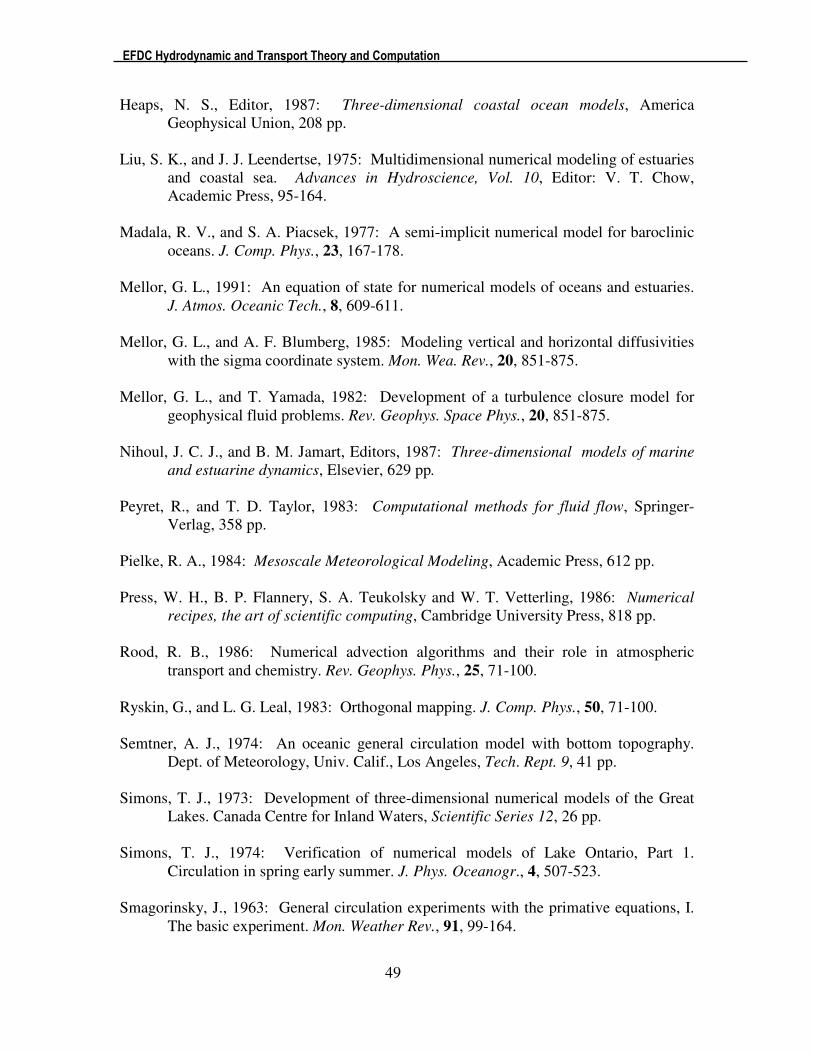
EFDC Hydrodynamic and Transport Theory and Computation
49
Heaps, N. S., Editor, 1987: Three-dimensional coastal ocean models, America
Geophysical Union, 208 pp.
Liu, S. K., and J. J. Leendertse, 1975: Multidimensional numerical modeling of estuaries
and coastal sea. Advances in Hydroscience, Vol. 10, Editor: V. T. Chow,
Academic Press, 95-164.
Madala, R. V., and S. A. Piacsek, 1977: A semi-implicit numerical model for baroclinic
oceans. J. Comp. Phys., 23, 167-178.
Mellor, G. L., 1991: An equation of state for numerical models of oceans and estuaries.
J. Atmos. Oceanic Tech., 8, 609-611.
Mellor, G. L., and A. F. Blumberg, 1985: Modeling vertical and horizontal diffusivities
with the sigma coordinate system. Mon. Wea. Rev., 20, 851-875.
Mellor, G. L., and T. Yamada, 1982: Development of a turbulence closure model for
geophysical fluid problems. Rev. Geophys. Space Phys., 20, 851-875.
Nihoul, J. C. J., and B. M. Jamart, Editors, 1987: Three-dimensional models of marine
and estuarine dynamics, Elsevier, 629 pp.
Peyret, R., and T. D. Taylor, 1983: Computational methods for fluid flow, Springer-
Verlag, 358 pp.
Pielke, R. A., 1984: Mesoscale Meteorological Modeling, Academic Press, 612 pp.
Press, W. H., B. P. Flannery, S. A. Teukolsky and W. T. Vetterling, 1986: Numerical
recipes, the art of scientific computing, Cambridge University Press, 818 pp.
Rood, R. B., 1986: Numerical advection algorithms and their role in atmospheric
transport and chemistry. Rev. Geophys. Phys., 25, 71-100.
Ryskin, G., and L. G. Leal, 1983: Orthogonal mapping. J. Comp. Phys., 50, 71-100.
Semtner, A. J., 1974: An oceanic general circulation model with bottom topography.
Dept. of Meteorology, Univ. Calif., Los Angeles, Tech. Rept. 9, 41 pp.
Simons, T. J., 1973: Development of three-dimensional numerical models of the Great
Lakes. Canada Centre for Inland Waters, Scientific Series 12, 26 pp.
Simons, T. J., 1974: Verification of numerical models of Lake Ontario, Part 1.
Circulation in spring early summer. J. Phys. Oceanogr., 4, 507-523.
Smagorinsky, J., 1963: General circulation experiments with the primative equations, I.
The basic experiment. Mon. Weather Rev., 91, 99-164.
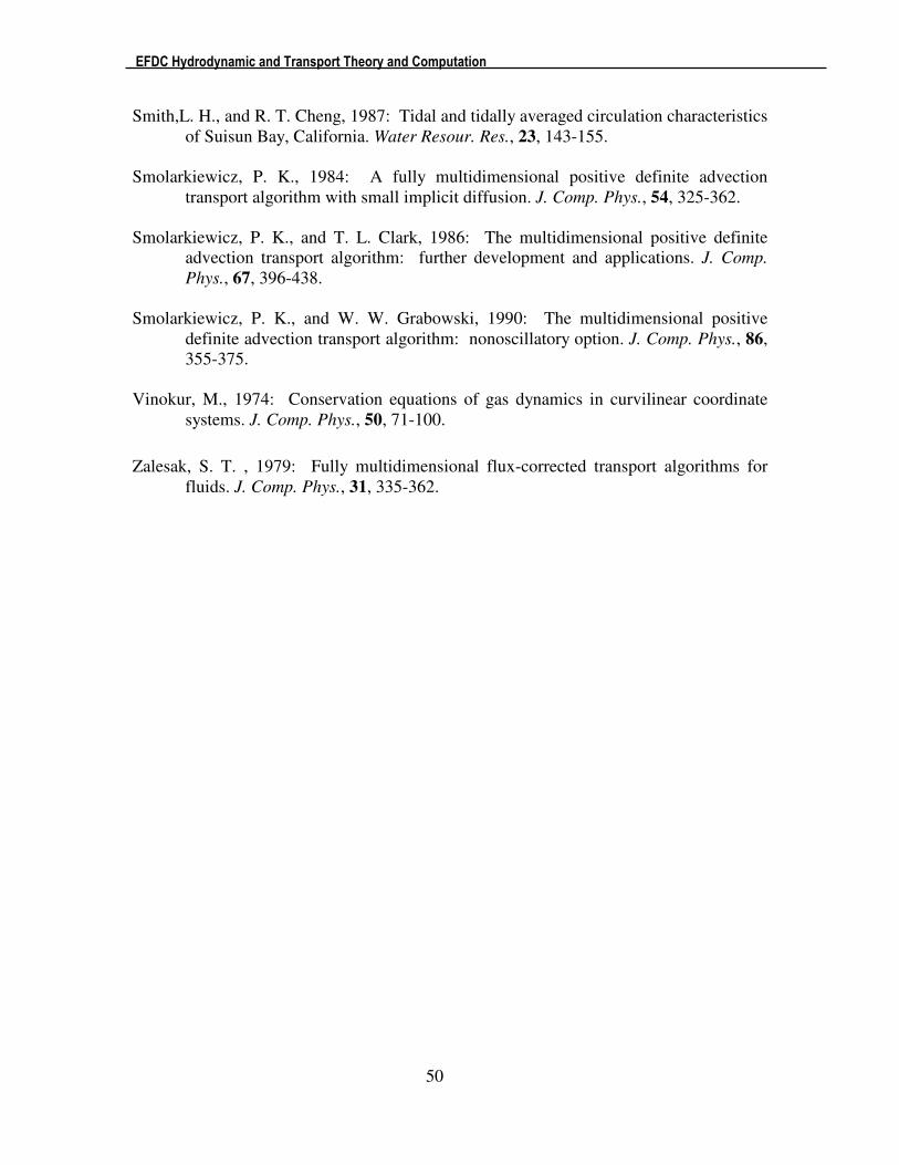
EFDC Hydrodynamic and Transport Theory and Computation
50
Smith,L. H., and R. T. Cheng, 1987: Tidal and tidally averaged circulation characteristics
of Suisun Bay, California. Water Resour. Res., 23, 143-155.
Smolarkiewicz, P. K., 1984: A fully multidimensional positive definite advection
transport algorithm with small implicit diffusion. J. Comp. Phys., 54, 325-362.
Smolarkiewicz, P. K., and T. L. Clark, 1986: The multidimensional positive definite
advection transport algorithm: further development and applications. J. Comp.
Phys., 67, 396-438.
Smolarkiewicz, P. K., and W. W. Grabowski, 1990: The multidimensional positive
definite advection transport algorithm: nonoscillatory option. J. Comp. Phys., 86,
355-375.
Vinokur, M., 1974: Conservation equations of gas dynamics in curvilinear coordinate
systems. J. Comp. Phys., 50, 71-100.
Zalesak, S. T. , 1979: Fully multidimensional flux-corrected transport algorithms for
fluids. J. Comp. Phys., 31, 335-362.
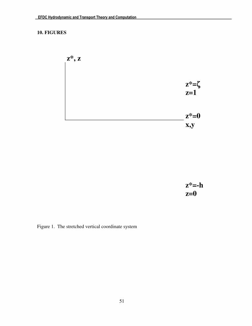
EFDC Hydrodynamic and Transport Theory and Computation
51
10. FIGURES
z*, z
z*=ζζζζ z=1
z*=0
x,y
z*=-h
z=0 Figure 1. The stretched vertical coordinate system
EFDC Hydrodynamic and Transport Theory and Computation
52
v v
u ζ,w,b u ζ,w,b u
v v
u ζ,w,b u ζ,w,b u
v v Figure 2. Free surface displacement centered horizontal grid.
_____ v,mx
(x-0.5,y+0.5) _____ v,mx
(x+0.5,y+0.5) _____
|
|
|
|
u,my
(x-1,y) ζ,b,m (x-0.5,y)
u,my
(x,y) ζ,b,m
(x+0.5,y) u,my
(x+1,y) |
|
|
|
_____ v,mx
(x-0.5,y-0.5) _____ v,mx
(x+0.5,y-0.5) _____
Figure 3. U-centered grid in the horizontal (x,y) plane.
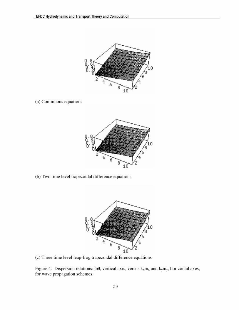
EFDC Hydrodynamic and Transport Theory and Computation
53
(a) Continuous equations
(b) Two time level trapezoidal difference equations
(c) Three time level leap-frog trapezoidal difference equations
Figure 4. Dispersion relations: ωθ, vertical axis, versus kxmx and kymy, horizontal axes,
for wave propagation schemes.
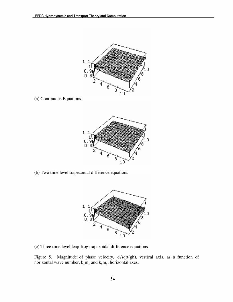
EFDC Hydrodynamic and Transport Theory and Computation
54
(a) Continuous Equations
(b) Two time level trapezoidal difference equations
(c) Three time level leap-frog trapezoidal difference equations
Figure 5. Magnitude of phase velocity, |c|/sqrt(gh), vertical axis, as a function of
horizontal wave number, kxmx and kymy, horizontal axes.
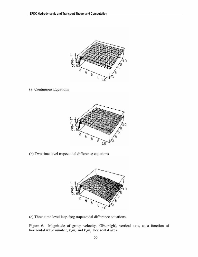
EFDC Hydrodynamic and Transport Theory and Computation
55
(a) Continuous Equations
(b) Two time level trapezoidal difference equations
(c) Three time level leap-frog trapezoidal difference equations
Figure 6. Magnitude of group velocity, |G|/sqrt(gh), vertical axis, as a function of
horizontal wave number, kxmx and kymy, horizontal axes.
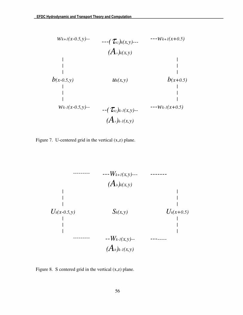
EFDC Hydrodynamic and Transport Theory and Computation
56
wk+1(x-0.5,y)-- ---(τxz)k(x,y)---
(Av)k(x,y)
---wk+1(x+0.5)
| | |
| | |
b(x-0.5,y) uk(x,y) b(x+0.5)
| | |
| | |
wk-1(x-0.5,y)-- --(τxz)k-1(x,y)--
(Av)k-1(x,y)
---wk-1(x+0.5)
Figure 7. U-centered grid in the vertical (x,z) plane.
--------- ---Wk+1(x,y)---
(Ab)k(x,y)
-------
| | |
| | |
Uk(x-0.5,y) Sk(x,y) Uk(x+0.5)
| | |
| | |
--------- --Wk-1(x,y)--
(Ab)k-1(x,y)
--------
Figure 8. S centered grid in the vertical (x,z) plane.
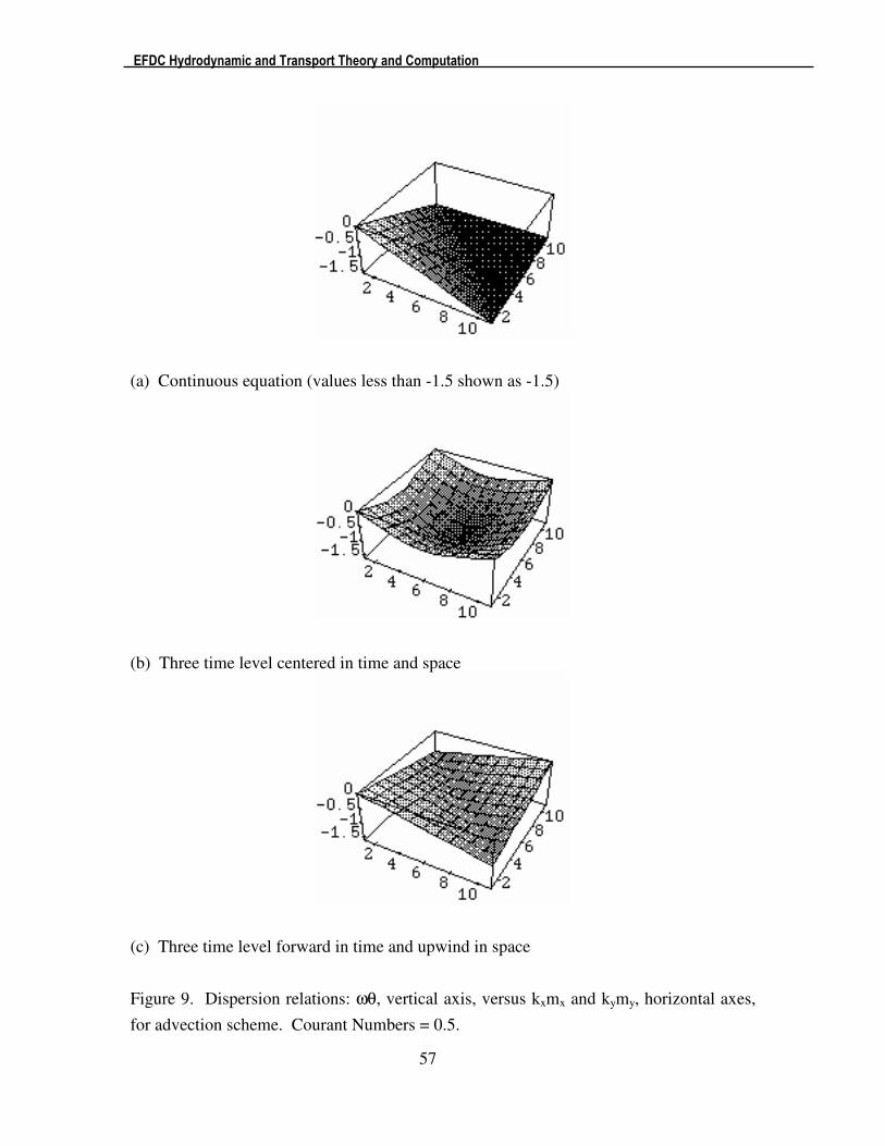
EFDC Hydrodynamic and Transport Theory and Computation
57
(a) Continuous equation (values less than -1.5 shown as -1.5)
(b) Three time level centered in time and space
(c) Three time level forward in time and upwind in space
Figure 9. Dispersion relations: ωθ, vertical axis, versus kxmx and kymy, horizontal axes,
for advection scheme. Courant Numbers = 0.5.
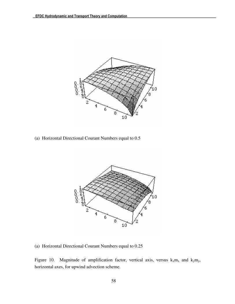
EFDC Hydrodynamic and Transport Theory and Computation
58
(a) Horizontal Directional Courant Numbers equal to 0.5
(a) Horizontal Directional Courant Numbers equal to 0.25
Figure 10. Magnitude of amplification factor, vertical axis, versus kxmx and kymy,
horizontal axes, for upwind advection scheme.
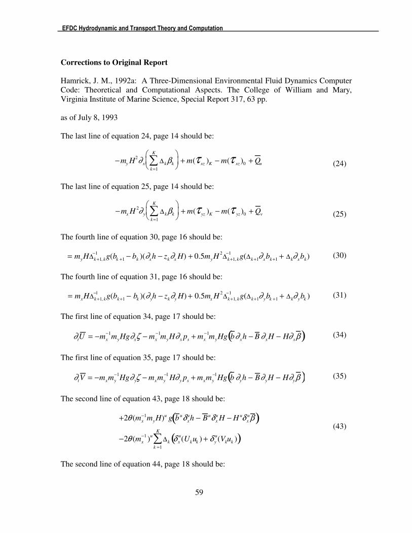
EFDC Hydrodynamic and Transport Theory and Computation
59
Corrections to Original Report
Hamrick, J. M., 1992a: A Three-Dimensional Environmental Fluid Dynamics Computer
Code: Theoretical and Computational Aspects. The College of William and Mary,
Virginia Institute of Marine Science, Special Report 317, 63 pp.
as of July 8, 1993
The last line of equation 24, page 14 should be:
−my H2∂ x ∆ kβk
k=1
K
∑
+ m(τ xz )K − m(τ xz )0 + Q u
(24)
The last line of equation 25, page 14 should be:
−mx H2∂ y ∆ kβk
k=1
K
∑
+ m(τ yz )K − m(τ yz)0 + Q v
(25)
The fourth line of equation 30, page 16 should be:
= myH∆k +1, k
−1g(bk +1 − bk )(∂xh − zk∂x H) + 0.5myH
2∆ k+1, k
−1g(∆k +1∂ xbk+1 + ∆k∂ xbk) (30)
The fourth line of equation 31, page 16 should be:
= mxH∆k +1, k
−1g(bk+1 − bk )(∂ yh − zk∂y H) + 0.5mx H
2∆k+1, k
−1g(∆ k+1∂ ybk +1 + ∆k∂ ybk ) (31)
The first line of equation 34, page 17 should be:
∂tU = −mx
−1myHg∂xζ − mx
−1myH∂ x ps + mx
−1myHg b ∂ xh − B ∂ xH − H∂ xβ ( ) (34)
The first line of equation 35, page 17 should be:
∂tV = −mxmy
−1Hg∂ yζ − mxmy
−1H∂ y ps + mxmy
−1Hg b ∂yh − B ∂ yH − H∂yβ ( ) (35)
The second line of equation 43, page 18 should be:
+2θ (mx
−1myH)u g b uδ x
uh − B uδ x
u H − H uδ x
uβ ( )
−2θ (mx
−1)
u∆k δ x
u(Ukuk ) + δ y
u(Vkuk )( )
k =1
K
∑
(43)
The second line of equation 44, page 18 should be:
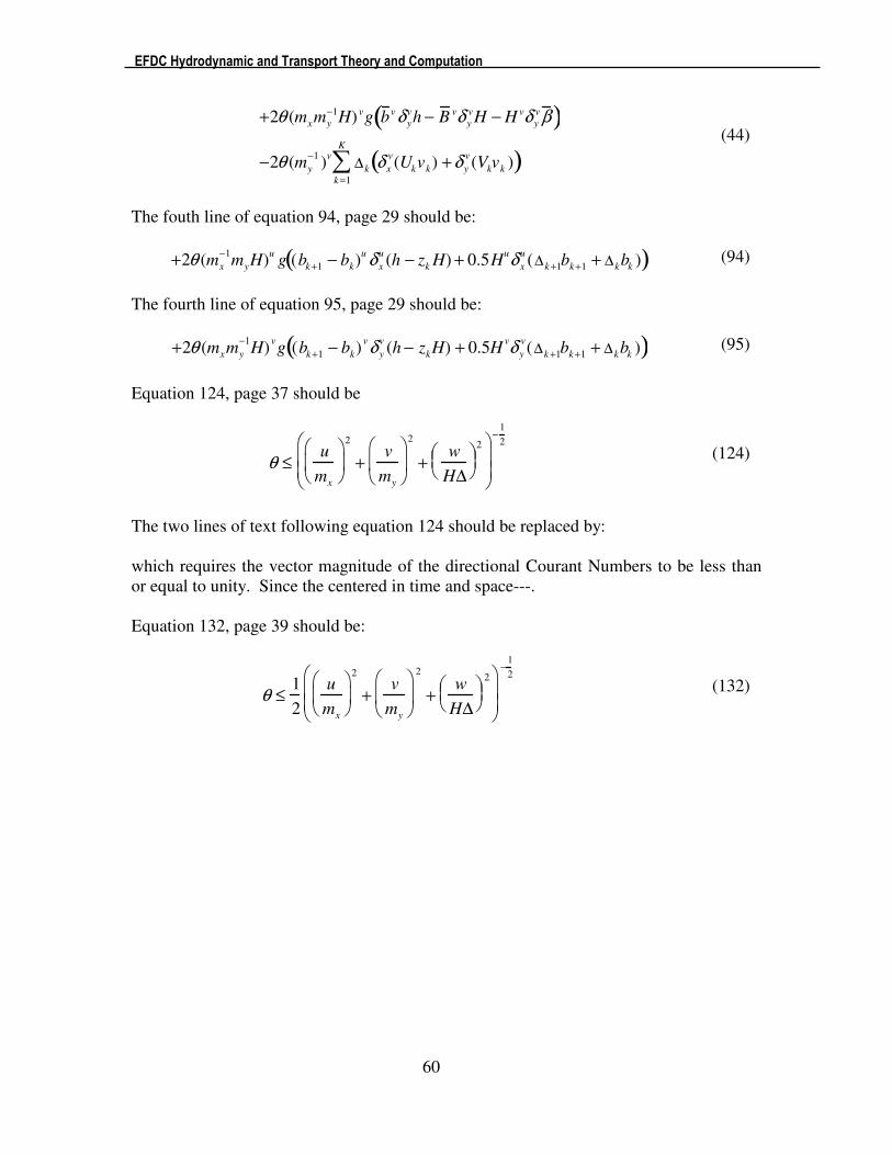
EFDC Hydrodynamic and Transport Theory and Computation
60
+2θ (mxmy
−1H) vg b vδ y
vh − B vδ y
vH − H vδ y
vβ ( )
−2θ (my
−1)
v∆k δ x
v(Ukvk) +δ y
v(Vkvk )( )
k =1
K
∑
(44)
The fouth line of equation 94, page 29 should be:
+2θ (mx
−1myH)
ug (bk+1 − bk)
u δ x
u(h − zk H) + 0.5H
uδ x
u(∆k +1bk+1 + ∆kbk )( ) (94)
The fourth line of equation 95, page 29 should be:
+2θ (mxmy
−1H)
vg (bk+1 − bk)
vδ y
v(h − zkH) + 0.5H
vδ y
v(∆k +1bk+1 + ∆kbk )( ) (95)
Equation 124, page 37 should be
θ ≤u
mx
2
+v
my
2
+w
H∆
2
−1
2
(124)
The two lines of text following equation 124 should be replaced by:
which requires the vector magnitude of the directional Courant Numbers to be less than
or equal to unity. Since the centered in time and space---.
Equation 132, page 39 should be:
θ ≤1
2
u
mx
2
+v
my
2
+w
H∆
2
−1
2
(132)