1

Finite Element Modeling and

Adaptive Refinement

John O. Dow

THE ESSENTIALS OF

For Beginning Analysts to Advanced Researchers in Solid Mechanics

CONTENTS

PREFACE xi

1 INTRODUCTION 1

1.1 Problem Defi nition 1 1.2 Overall Objectives 3 1.3 Specifi c Tasks 3 1.4 The Central Role of the Interpolation Functions 4 1.5 A Closer Look at the Interpolation Functions 5 1.6 Physically Interpretable Interpolation

Functions in Action 7 1.7 The Overall Signifi cance of the Physically Interpretable Notation 8 1.8 Examples of Model Refi nement and the Need for Adaptive Refi nement 8 1.9 Examples of Adaptive Refi nement and Error Analysis 10 1.10 Summary 13 1.11 References 14

2 AN OVERVIEW OF FINITE ELEMENT MODELING CHARACTERISTICS 15

2.1 Introduction 15 2.2 Characteristics of Exact Finite Element Results 18 2.3 More Demanding Loading Conditions 19 2.4 Discretization Errors in an Initial Model 21 2.5 Error Reduction and Uniform Refi nement 23 2.6 Error Reduction and Adaptive Refi nement 25 2.7 The Effect of Element Modeling Capability on Discretization Errors 27 2.8 Summary and Future Applications 30 2.9 References 31

2A ELEMENTS OF TWO-DIMENSIONAL MODELING 33

2A.1 Introduction 332A.2 SubModeling Refi nement Strategy 342A.3 Initial Model 35

v

vi • CONTENTS

2A.4 Adaptive Refi nement Results 362A.5 Summary 372A.6 References 38

2B EXACT SOLUTIONS FOR TWO LONGITUDINAL BAR PROBLEMS 39

2B.1 Introduction 392B.2 General Solution of the Governing Differential Equation 402B.3 Application of a Free Boundary Condition 402B.4 Second Application of Separation of Variables 412B.5 Solution for a Constant Distributed Load 412B.6 Solution for a Linearly Varying Distributed Load 422B.7 Summary 44

3 IDENTIFICATION OF FINITE ELEMENT STRAIN MODELING CAPABILITIES 45

3.1 Introduction 45 3.2 Identifi cation of the Strain Modeling Capabilities

of a Three-Node Bar Element 47 3.3 An Introduction to Physically Interpretable Interpolation Polynomials 48 3.4 Identifi cation of the Physically Interpretable Coeffi cients 49 3.5 The Decomposition of Element Displacements into Strain Components 51 3.6 A Common Basis for the Finite Element and Finite

Difference Methods 53 3.7 Modeling Capabilities of the Four-Node Bar Element 55 3.8 Identifi cation and Evaluation of Element Behavior 56 3.9 Evaluation of a Two-Dimensional Strain Model 59 3.10 Analysis by Inspection in Two Dimensions 63 3.11 Summary and Conclusion 65 3.12 Reference 66

4 THE SOURCE AND QUANTIFICATION OF DISCRETIZATION ERRORS 67

4.1 Introduction 67 4.2 Background Concepts—The Residual Approach to Error Analysis 69 4.3 Quantifying the Failure to Satisfy Point-Wise Equilibrium 71 4.4 Every Finite Element Solution is an Exact Solution to Some Problem 76 4.5 Summary and Conclusion 78 4.6 Reference 78

5 MODELING INEFFICIENCY IN IRREGULAR ISOPARAMETRIC ELEMENTS 79

5.1 Introduction 79 5.2 An Overview of Isoparametric Element Strain Modeling Characteristics 81 5.3 Essential Elements of the Isoparametric Method 83

CONTENTS • vii

5.4 The Source of Strain Modeling Errors in Isoparametric Elements 84

5.5 Strain Modeling Characteristics of Isoparametric Elements 87 5.6 Modeling Errors in Irregular Isoparametric Elements 89 5.7 Results for a Series of Uniform Refi nements 91 5.8 Summary and Conclusion 93 5.9 References 94

6 INTRODUCTION TO ADAPTIVE REFINEMENT 95

6.1 Introduction 95 6.2 Physically Interpretable Error Estimators 96 6.3 A Model Refi nement Strategy 97 6.4 A Demonstration of Uniform Refi nement 97 6.5 A Demonstration of Adaptive Refi nement 101 6.6 An Application of an Absolute Error Estimator 103 6.7 Summary 106 6.8 References 107

7 STRAIN ENERGY-BASED ERROR ESTIMATORS—THE Z/Z ERROR ESTIMATOR 109

7.1 Introduction 109 7.2 The Basis of the Z/Z Error Estimator—A Smoothed

Strain Representation 110 7.3 The Z/Z Elemental Strain Energy Error Estimator 112 7.4 The Z/Z Error Estimator 113 7.5 A Modifi ed Locally Normalized Z/Z Error Estimator 114 7.6 A Demonstration of the Z/Z Error Estimator 114 7.7 A Demonstration of Adaptive Refi nement 119 7.8 Summary and Conclusion 123 7.9 References 124

7A GAUSS POINTS, SUPER CONVERGENT STRAINS, AND CHEBYSHEV POLYNOMIALS 125

7A.1 Introduction 1257A.2 Modeling Behavior of Three-Node Elements 1267A.3 Gauss Points and Chebyshev Polynomials 1287A.4 References 129

7B AN UNSUCCESSFUL EXAMPLE OF ADAPTIVE REFINEMENT 131

7B.1 Introduction 1317B.2 Example 1 1317B.3 Example 2 1327B.4 Summary 135

viii • CONTENTS

8 A HIGH RESOLUTION POINT-WISE RESIDUAL ERROR ESTIMATOR 137

8.1 Introduction 137 8.2 An Overview of the Point-Wise Residual Error Estimator 139 8.3 The Theoretical Basis for the Point-Wise Residual Error Estimator 141 8.4 Computation of the Point-Wise Residual Error Estimator 143 8.5 Formulation of the Finite Difference Operators 144 8.6 The Formulation of the Point-Wise Residual Error Estimator 147 8.7 A Demonstration of the Point-Wise Finite Difference Error Estimator 148 8.8 A Demonstration of Adaptive Refi nement 152 8.9 A Temptation to Avoid and a Reason for using Child Meshes 156 8.10 Summary and Conclusion 156 8.11 Reference 157

9 MODELING CHARACTERISTICS AND EFFICIENCIES OF HIGHER ORDER ELEMENTS 159

9.1 Introduction 159 9.2 Adaptive Refi nement Examples (4.0% Termination Criterion) 161 9.3 Adaptive Refi nement Examples (0.4% Termination Criterion) 165 9.4 In-Situ Identifi cation of the Five-Node Element Modeling Behavior 167 9.5 Strain Contributions of the Basis Set Components 171 9.6 Comparative Modeling Behavior of Four-Node Elements 173 9.7 Summary, Conclusion, and Recommendations for Future Work 185

10 FORMULATION OF A 10-NODE QUADRATIC STRAIN ELEMENT 189

10.1 Introduction 189 10.2 Identifi cation of the Linearly Independent Strain Gradient Quantities 191 10.3 Identifi cation of the Elemental Strain Modeling Characteristics 193 10.4 Formulation of the Strain Energy Expression 196 10.5 Identifi cation and Evaluation of the Required Integrals 198 10.6 Expansion of the Strain Energy Kernel 199 10.7 Formulation of the Stiffness Matrix 199 10.8 Summary and Conclusion 203

10A A NUMERICAL EXAMPLE FOR A 10-NODE STIFFNESS MATRIX 205

10A.1 Introduction 205 10A.2 Element Geometry and Nodal Numbering 206 10A.3 Formulation of the Transformation to Nodal Displacement

Coordinates 206 10A.4 Formulation and Evaluation of the Strain Energy Expression 212 10A.5 Formulation of the Stiffness Matrix 215 10A.6 Summary and Conclusion 217

CONTENTS • ix

10B MATLAB FORMULATION OF THE 10-NODE ELEMENT STIFFNESS MATRIX 223

10B.1 Introduction 223 10B.2 Driver Program for Forming the Stiffness

Matrix for a 10-Node Element 224 10B.3 Form Phi and Phi Inverse for 10-Node Element 227 10B.4 Form Integrals in Stiffness Matrix Using Green’s Theorem 228 10B.5 Form Strain Energy Kernel for 10-Node Element 232 10B.6 Plot Geometry and Nodes for 10-Node Element 236 10B.7 Function to Transform Matlab Matrices to Form for Use in Word 237

11 PERFORMANCE-BASED REFINEMENT GUIDES 239

11.1 Introduction 239 11.2 Theoretical Overview for Finite Difference Smoothing 241 11.3 Development of the Refi nement Guide 244 11.4 Problem Description 245 11.5 Examples of Adaptive Refi nement 247 11.6 An Effi cient Refi nement Guide Based on Nodal Averaging 251 11.7 Further Comparisons of the Refi nement Guides 254 11.8 Summary and Conclusion 257 11.9 References 258

12 SUMMARY AND RESEARCH RECOMMENDATIONS 259

12.1 Introduction 259 12.2 An Overview of Advances in Adaptive Refi nement 259 12.3 Displacement Interpolation Functions Revisited: A Reinterpretation 261 12.4 Advances in the Finite Element Method 262 12.5 Advances in the Finite Difference Method 264 12.6 Recommendations for Future Work and Research Opportunities 264 12.7 Reference 265

INDEX 267

PREFACE

As the title declares, this book is largely concerned with fi nite element modeling and the improve-ment of these models with adaptive refi nement. The intended audience for this book consists of readers who are either early in their technical careers or mature users and researchers in computa-tional mechanics.

The width of the intended audience for this book makes it unique and presents an interesting challenge to the author. There is only one way a technical book (versus a popularization of a techni-cal topic) can address such a wide audience. The book must present developments that simplify, improve, and extend the discipline.

This book contains material that accomplishes these ends. The fi nite element method is sim-plifi ed, improved, and extended. Furthermore, the fi nite element and fi nite difference methods are unifi ed as a result of these developments. These capabilities are used here to simplify, improve, and extend the adaptive refi nement process.

These capabilities derived from earlier work done by the author, his colleagues, and graduate students in which the continuum properties are extracted from frames and trusses. This was done so it could be determined, with a minimum of analysis, whether the torsion and fl exure was uncoupled in lattices for the space station in order to reduce the effect from the docking of the Space Shuttle. In other words, this process inverted the fi nite element method.

Later, the author recognized that the process for extracting continuum properties for skeletal structures could be inverted to produce an approach that both simplifi ed and improved the formula-tion of fi nite element stiffness matrices. In fact, this new approach for forming fi nite element stiff-ness matrices renders the isoparametric formulation procedure obsolete as is discussed in Chapter 3.

The key to this new formulation procedure is the recognition that the displacement inter-polation functions are actually truncated Taylor series expansions whose coeffi cients could be expressed in terms of physically interpretable quantities. Later still, it was recognized that fi nite difference templates or operators were embedded in the new element formulation process. These observations provide the basis for this book and make its contents accessible for the breadth of the intended audience.

Recently, this work was extended to create new types of error estimators and refi nement guides. In addition to being easy to compute because they are point-wise quantities, the new error estimators report the error in terms of quantities that are basic to continuum mechanics.

xi

xii • PREFACE

One of the new error estimators quantifi es the errors in terms of strains. The other new error estimator reports the errors with a metric related to the applied loads. The evaluation of an element in terms of quantities of direct interest in continuum mechanics contrasts with the strain energy metric used in the well-known error estimator developed by Zienkiewicz and Zhu (Z/Z), which is of secondary interest in analysis.

The new in situ refi nement guides differ from previous refi nement guides because they are based on physical principles instead of correlations with error estimates. In the new approach, the modeling defi ciencies in individual elements are identifi ed by comparing the modeling capabilities of the elements to an estimate of the exact solution over the domain of the element using physically interpretable notation.

This book integrates these recent developments to adaptive refi nement with earlier improve-ments to the fi nite element and fi nite difference methods. One-dimensional problems are used to illustrate the underlying concepts. This is done so the ideas are not submerged in the large amount of data produced in multidimensional problems. As a result, the presentation is compact and the basic ideas are easy to understand.

Most of the background material presented here for the one-dimensional case is available in higher dimensions in my previous book entitled, A Unifi ed Approach to the Finite Element Method and Error Analysis Procedures. Only the recent improvements to error estimators and refi nement guides are not included in the previous book. Extensions of these topics are identifi ed as possible research avenues in the fi nal section of the concluding chapter of this book.

This book is accessible to someone new to fi nite element analysis because it contains the neces-sary background information from the following topics:

1. Taylor series expansions from undergraduate calculus.2. The idea of basis functions from linear algebra.3. Defi nition of rigid body motions from linear elasticity.4. Defi nition of strains from mechanics of materials.5. Integration over an area using Green’s theorem.6. Solution of simultaneous equations.

This book is useful to advanced researchers because it presents the following topics from a fresh point of view:

1. An element formulation process that makes the isoparametric approach obsolete.2. Procedures for evaluating the modeling capabilities of individual elements during the formu-

lation procedure.3. Improvements and extensions to the fi nite difference method.4. New types of error estimators.5. A new a posteriori approach for identifying the level of refi nement needed to rapidly improve fi nite element models.

6. The identifi cation of Gauss points in terms of Chebyshev polynomials.

PREFACE • xiii

A synopsis of each of the 12 Chapters that comprise this book follows.

CHAPTER 1: INTRODUCTION

Chapter 1 provides an overview of the book and major topics contained in the book, namely, error analysis and adaptive refi nement. The two problems facing an analyst using an approximate solution technique are identifi ed in the fi rst section as: (1) the need to assess the accuracy of the approxi-mate solution and (2) the identifi cation of modifi cations to the model that will produce results of the desired accuracy. The overall objectives and the specifi c tasks that are required to produce sat-isfactory results with the fi nite element method are presented. The defi ciencies in a fi nite element model are identifi ed as the inability of the simple polynomial basis functions of the individual fi nite elements to capture the complexity of the exact solution being sought. The errors are quantifi ed by identifying metrics that measure the amount by which the approximations produced by the indi-vidual elements fail to capture the exact solution. Then, procedures that use physically interpre-table interpolation polynomials to identify the changes needed to rapidly improve the model are presented. These techniques are demonstrated and compared to earlier error analysis and adaptive refi nement procedures in the following chapters.

CHAPTER 2: AN OVERVIEW OF FINITE ELEMENT MODELING CHARACTERISTICS

Chapter 2 provides an intuitive introduction to the errors that exist in fi nite element results as a con-sequence of replacing the continuum with a discrete number of fi nite elements. These discretization errors are produced when the exact solution is too complex to be represented by the interpolation functions of the individual elements. The discretization errors are literally seen in the fi nite element results as interelement jumps in the strain distributions. The interelement jumps provide an ideal met-ric for an error estimator and a termination criterion. On one hand, the interelement jumps are shown in Chapter 4 to be aggregated residual quantities that measure the failure of the fi nite element solution to satisfy the governing differential equation being approximated. On the other hand, the interelement jumps in the strain express the errors in terms of quantities that are being sought in computational mechanics, namely, strain. This means, for example, that if the material being analyzed fails at 1000 units, the magnitude of the error can be interpreted in terms of the failure criterion.

CHAPTER 3: STRAIN MODELING CAPABILITIES OF INDIVIDUAL FINITE ELEMENTS

Chapter 3 presents a procedure for identifying the strain modeling capabilities of individual fi nite ele-ments during the formulation of the element stiffness matrix. This capability is made possible by the recognition that fi nite element interpolation polynomials can be interpreted as Taylor series expansions

xiv • PREFACE

whose coeffi cients can be expressed in terms of quantities that produce displacements in the con-tinuum, namely, rigid body motions, constant strains, and derivatives of the strain components. This physically interpretable notation reduces the level of mathematics required for the development of the fi nite element method, error analysis, and adaptive refi nement processes to that which is learned in undergraduate calculus. That is to say, functional analysis is not needed. The advances that this nota-tion brings to computational mechanics are discussed at length in the concluding chapter.

CHAPTER 4: THE SOURCE AND QUANTIFICATION OF DISCRETIZATION ERRORS

Chapter 4 identifi es the source of the interelement jumps in the nodal strains that quantify the dis-cretization errors in fi nite element solutions. The interelement jumps consist of the nodal equivalent values of the point wise residuals on the domain of an element. The residuals quantify the failure of the fi nite element solution to satisfy the governing differential equation being solved. This under-standing of the source of the discretization errors allows error estimators and refi nement guides to be based on fi rst principles instead of on a correlation with secondary quantities, such as strain energy. The refi nement guides that utilize this knowledge and the physically interpretable notation presented in Chapter 3 are developed in Chapter 11. As discussed in the concluding chapter, the availability of refi nement guides based on fi rst principles changes the structure of the adaptive refi nement process.

CHAPTER 5: MODELING INEFFICIENCIES IN IRREGULAR ISOPARAMETRIC ELEMENTS

Chapter 5 introduces a better and more effi cient way to form stiffness matrices than the isopara-metric approach. The stiffness matrices formed using the physically interpretable strain gradient notation are simpler to compute because signifi cantly fewer integrals must be evaluated and iso-parametric mappings are not required. Furthermore, the way in which the isoparametric mapping causes modeling errors in distorted isoparametric elements is demonstrated. The ineffi ciencies that exist in fi nite element models formed with distorted isoparametric elements are demonstrated with examples. In addition to identifying a source of errors in fi nite element models, this chapter further demonstrates the effi cacy of strain gradient notation.

CHAPTER 6: INTRODUCTION TO ADAPTIVE REFINEMENT

Chapter 6 introduces and applies the adaptive refi nement process. The presentation is designed to identify the three necessary components of adaptive refi nement: (1) an error estimator, (2) a termina-tion criterion, and (3) a refi nement strategy. In this demonstration of adaptive refi nement, the jumps in the interelement nodal strain are used as the error estimator and to defi ne the termination criteria. A simple refi nement strategy that divides an element that fails the termination criteria into two

PREFACE • xv

elements is used in this demonstration. A refi nement guide based on fi rst principles is developed and presented in Chapter 12. In one demonstration of adaptive refi nement presented in this chapter, the inaccuracies in the strain representation for distorted isoparametric elements that have been identi-fi ed in the previous chapter are shown to produce ineffi cient fi nite element models.

CHAPTER 7: STRAIN ENERGY-BASED ERROR ESTIMATORS

Chapter 7 introduces and demonstrates the fi rst practical error estimator. At the heart of this pro-cedure, which was developed by Zienkiewicz and Zhu, is the formation of a smoothed strain rep-resentation that is assumed to be closer to the exact solution than the discontinuous fi nite element result. The error is estimated by computing the difference in the strain energy between the smoothed solution and the fi nite element solution. This error estimator is put on a solid theoretical foundation in this chapter by showing that the smoothed solution is, indeed, closer to the exact result than the fi nite element solution. The idea of an improved solution that is closer to the exact solution than the discontinuous fi nite element solution is extended in Chapter 11 to form a refi nement guide based on fi rst principles that signifi cantly improves the adaptive refi nement process.

CHAPTER 8: A HIGH RESOLUTION, POINT-WISE RESIDUAL ERROR ESTIMATOR

Chapter 8 develops and applies a high resolution, point-wise error estimator that forms a residual quantity using fi nite difference operators. This error estimator identifi es the magnitude of the failure of the fi nite element solution to satisfy the fi nite difference approximation of the governing differ-ential equation at individual points. The rationale behind this error estimator is the idea that both the fi nite element and the fi nite difference methods attempt to solve the same problem with differ-ent approaches. Since both solutions will approach the exact solution in the limit, the residual will approach zero as the solution gets close to the exact solution. However, the primary importance of this development is the demonstration that the fi nite element and the fi nite difference methods share the same Taylor series basis. This means that fi nite difference templates can be applied to any point on any fi nite element model. In addition to possibly infusing the fi nite difference method with new life as it pertains to solving solid mechanics problems, the use of fi nite difference templates provides an alternative, highly effective way to form a smoothed solution for use in the refi nement guide that is developed in Chapter 11.

CHAPTER 9: MODELING CHARACTERISTICS AND EFFICIENCIES OF HIGHER ORDER ELEMENTS

Chapter 9 demonstrates that higher order elements are more effi cient on a node-for-node basis than lower order elements when they represent complex strain distributions with stringent termination

xvi • PREFACE

criteria. This behavior is identifi ed by replacing single fi ve-node bar elements with increasing numbers of four-node elements in a problem with a complex strain distribution. The lower order elements com-pensate for their inability to represent the additional strain states that higher order elements can repre-sent with a fi nite representation of the higher order strain representations. That is to say, the curvature in the four-node elements changes in order to represent the change of curvature that a single fi ve-node element can represent. This result is exploited to produce refi nement guides based on fi rst principles that are developed in Chapter 11. As we will see, this new approach to forming refi nement guides allows the role of the error estimator to be simplifi ed. It need only serve as a termination criterion. It need not serve as the basis for the degree of refi nement needed to improve a fi nite element model.

CHAPTER 10: FORMULATION OF A 10-NODE QUADRATIC STRAIN ELEMENT

Chapter 10 presents the formulation of a 10-node fi nite element using the physically interpretable strain gradient notation for two primary reasons. The fi rst is to make this higher order element avail-able because of the effi ciencies that were demonstrated for higher order elements in the previous chapter. The second is to demonstrate the advantages of using the strain gradient approach over the isoparametric approach. These advantages include: (1) the visual identifi cation of the strain model-ing capabilities of the 10-node element, (2) the clarifi cation of the role and use of the compatibility equation, (3) the need to evaluate signifi cantly fewer integrals than are required to form an isopara-metric element (15 versus 210), and (4) the fact that the required integrals have a simple form and can be integrated exactly with little diffi culty. Two Appendices are associated with this chapter. The fi rst provides a numerical example for a 10-node element. Its purpose is to provide a sample so that the implementation can be checked. The second Appendix is comprised of a heavily annotated set of Matlab m-fi les for forming the stiffness matrix presented in the fi rst Appendix. It is designed to provide the details for forming strain gradient based fi nite elements stiffness matrices.

CHAPTER 11: PERFORMANCE-BASED REFINEMENT GUIDES

Chapter 11 develops a new type of refi nement guide that is based on fi rst principles instead of a cor-relation with the error estimator. This approach to refi nement changes the structure of the adaptive refi nement process because the error estimator now needs only to function as a termination criterion since it is not directly involved with identifying the level of refi nement needed. This means that an error estimator can be chosen that is directly related to the problem being solved. For example, the use of the interelement jumps in strain as the error estimator provides a metric, that is, strains, that can be directly related to a failure criterion.

This approach to model refi nement, fi rst, decomposes an improved strain distribution through the use of strain gradient notation to estimate the participation of the higher order strain representa-tions that the elements in the fi nite element model cannot represent. These modeling defi ciencies are then compared to the modeling characteristics of the elements that make up the fi nite element model

PREFACE • xvii

in order to identify the level of refi nement needed to satisfy the termination criterion by using the knowledge developed in Chapter 9 concerning the behavior of higher order elements.

CHAPTER 12: SUMMARY AND RESEARCH OPPORTUNITIES

Chapter 12 provides a list of research opportunities associated with multidimensional problems that are extensions of the developments presented here. These opportunities are given in such a way that they constitute a summary of the developments contained in this book.

In closing, I wish to thank the approximately 25 graduate students that worked on these related top-ics and acknowledge their hard work and innumerable contributions to these advances in the fi nite element method, the fi nite difference method, and adaptive refi nement. Without their contribution this book could not have been written.

1

CHAPTER 1

INTRODUCTION

1.1 PROBLEM DEFINITION

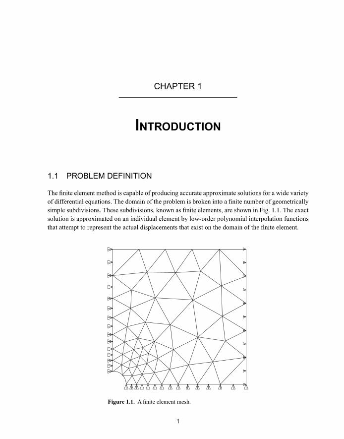
The fi nite element method is capable of producing accurate approximate solutions for a wide variety of differential equations. The domain of the problem is broken into a fi nite number of geometrically simple subdivisions. These subdivisions, known as fi nite elements, are shown in Fig. 1.1. The exact solution is approximated on an individual element by low-order polynomial interpolation functions that attempt to represent the actual displacements that exist on the domain of the fi nite element.

Figure 1.1. A fi nite element mesh.

2 • THE ESSENTIALS OF FINITE ELEMENT MODELING AND ADAPTIVE REFINEMENT

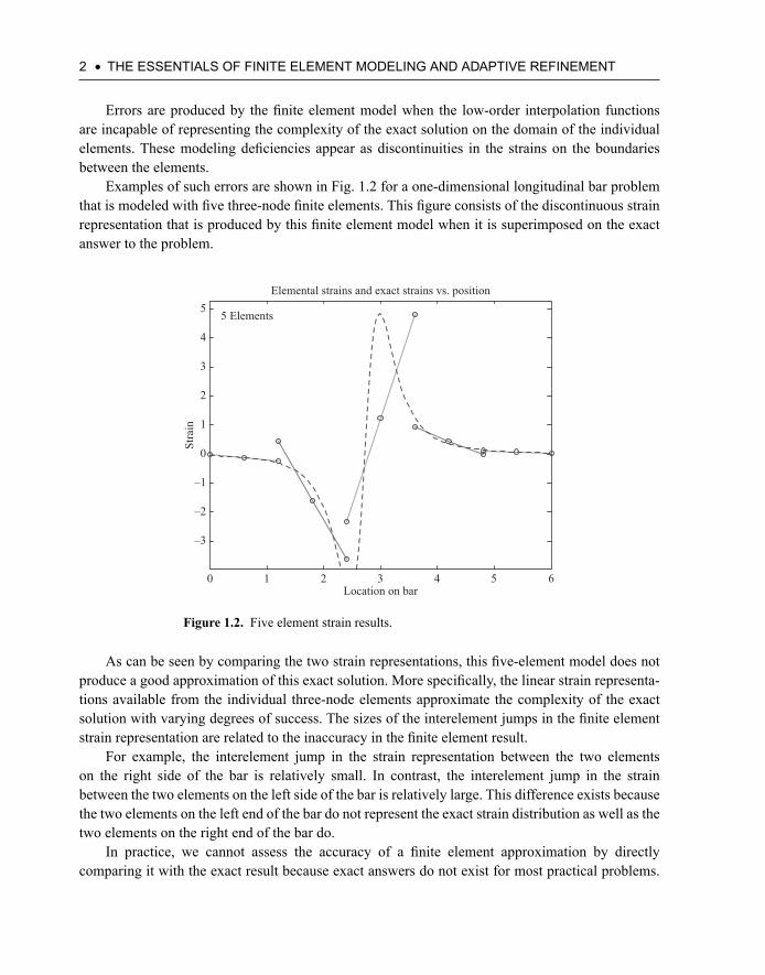
Errors are produced by the fi nite element model when the low-order interpolation functions are incapable of representing the complexity of the exact solution on the domain of the individual elements. These modeling defi ciencies appear as discontinuities in the strains on the boundaries between the elements.

Examples of such errors are shown in Fig. 1.2 for a one-dimensional longitudinal bar problem that is modeled with fi ve three-node fi nite elements. This fi gure consists of the discontinuous strain representation that is produced by this fi nite element model when it is superimposed on the exact answer to the problem.

0 1 2 3 4 5 6

–3

–2

–1

0

1

2

3

4

5Elemental strains and exact strains vs. position

Location on bar

Stra

in

5 Elements

Figure 1.2. Five element strain results.

As can be seen by comparing the two strain representations, this fi ve-element model does not produce a good approximation of this exact solution. More specifi cally, the linear strain representa-tions available from the individual three-node elements approximate the complexity of the exact solution with varying degrees of success. The sizes of the interelement jumps in the fi nite element strain representation are related to the inaccuracy in the fi nite element result.

For example, the interelement jump in the strain representation between the two elements on the right side of the bar is relatively small. In contrast, the interelement jump in the strain between the two elements on the left side of the bar is relatively large. This difference exists because the two elements on the left end of the bar do not represent the exact strain distribution as well as the two elements on the right end of the bar do.

In practice, we cannot assess the accuracy of a fi nite element approximation by directly comparing it with the exact result because exact answers do not exist for most practical problems.

INTRODUCTION • 3

As a consequence, we are faced with two diffi cult problems in order to produce approximate results with an acceptable level of accuracy. The fi rst problem requires that we assess the accu-racy of the fi nite element approximation. The second problem requires that we modify the existing fi nite element model so that it effi ciently produces a result that is suffi ciently accurate.

1.2 OVERALL OBJECTIVES

The overall objectives of this work are the following:

1. To develop a procedure based on basic or fi rst principles of continuum mechanics for identi-fying refi nements to the fi nite element model that will improve the accuracy of the resulting solution.

2. To present procedures for estimating the errors in a fi nite element result in terms of quantities that are meaningful to the analyst; for example, the errors are given as a percentage of a critical strain value.

3. To give an overview of different error analysis procedures.4. To demonstrate the improved modeling effi ciency that results from using higher order fi nite

elements to represent complex strain distributions.5. To present an improved and more intuitive element formulation procedure.

The fi rst two objectives apply directly to the components of the adaptive refi nement process that are developed here. The last three objectives provide the necessary background and developments that serve as the basis for the error estimators and refi nement guides presented in this work.

1.3 SPECIFIC TASKS

Since we cannot identify the errors in a fi nite element result by a direct comparison with an exact result, we must assess the accuracy of the fi nite element approximation and improve the model indi-rectly. The indirect assessment and refi nement of the existing model is accomplished with informa-tion that is available to us, namely, the modeling characteristics of the individual fi nite elements and the results produced by the fi nite element model.

The overall objectives of this work are accomplished with the following seven ambitious tasks:

1. Identify the two sources of errors in fi nite element models, namely, the modeling errors that may exist in individual elements and the inability of individual elements to capture the com-plexity of the solution being sought (Chapters 2, 3, 4, 5, 10, and 11).

2. Relate the modeling errors and the interelement jumps in the fi nite element result (Chapters 4 and 9).

4 • THE ESSENTIALS OF FINITE ELEMENT MODELING AND ADAPTIVE REFINEMENT

3. Present the two primary approaches to error analysis, namely, the residual and the recovery approaches (Chapters 4, 6, and 7).

4. Develop a new simplifi ed approach to error analysis that integrates the residual and recovery approaches to error analysis (Chapters 7 and 8).

5. Develop a new approach for forming refi nement guides to improve fi nite element models that is based on fi rst principles and not on a correlation based on the magnitudes of the elemental error estimates, that is, the errors are identifi ed by comparing an estimate of the emerging exact solution with the modeling capability of an individual element (Chapter 11).

6. Demonstrate that the fi nite element and the fi nite difference methods are directly related by showing that fi nite element interpolation functions and fi nite difference derivative approxi-mations can be formed from the same truncated Taylor series expansions (Chapters 3, 5, and 10).

7. Present an improved procedure for forming fi nite element stiffness matrices by specializing the displacement interpolation functions for solid mechanics problems by using physically interpretable coeffi cients expressed in terms of the quantities that produce displacements in the continuum, namely, rigid body motions and strains (Chapters 3 and 5).

1.4 THE CENTRAL ROLE OF THE INTERPOLATION FUNCTIONS

As pointed out in Section 1.1, the fi nite element method attempts to represent portions of the exact solution on the domains of the individual elements with low-order polynomial interpolation func-tions. If the exact solution is too complex over the domain of an element for the element’s interpola-tion function to represent, errors will occur in the fi nite element solution.

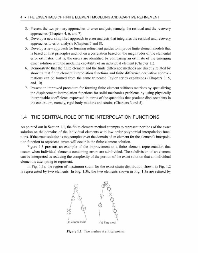
Figure 1.3 presents an example of the improvement to a fi nite element representation that occurs when individual elements containing errors are subdivided. The subdivision of an element can be interpreted as reducing the complexity of the portion of the exact solution that an individual element is attempting to represent.

In Fig. 1.3a, the region of maximum strain for the exact strain distribution shown in Fig. 1.2 is represented by two elements. In Fig. 1.3b, the two elements shown in Fig. 1.3a are refi ned by

Figure 1.3. Two meshes at critical points.

(a) Coarse mesh (b) Fine mesh

INTRODUCTION • 5

subdividing each of them into four elements. This means that each element in Fig. 1.3b is being asked to represent a smaller, less complex portion of the exact solution than are the individual elements inFig. 1.3a.

When the two fi nite element representations of the points of maximum strain shown in Fig. 1.3 are compared with the exact solution, the refi ned model produces a better result than does the initial model. As a consequence of the improvement to the model, the interelement jumps in the strain are smaller for this better representation of the exact solution. It should be noted that the Weierstrass approximation theorem gives the fi nite element method a solid theoretical foundation1 and guaran-tees that the refi nement process will improve the fi nite element model.

1.5 A CLOSER LOOK AT THE INTERPOLATION FUNCTIONS

The overview of the way a fi nite element model forms an approximate solution presented in the previous section identifi es that the heart of the fi nite element method is contained in the interpolation functions. The tasks listed in Section 1.3 are achieved by fi rst recognizing that the interpolation polynomials are truncated Taylor series expansions. This recognition performs two functions. First, it identifi es that the fi nite element and the fi nite difference methods have a common basis.2 The identifi cation of a common basis for these two powerful approximation techniques pro-vides a starting point for the development of the point-wise error estimator presented in Chapter 8 and for the refi nement guides based on fi rst principles that are presented in Chapter 10.

Second, this recognition allows the coeffi cients of the interpolation functions to be expressed in terms of rigid body motions and strain quantities. As a result, the displacements produced by the interpolation functions are expressed in terms of the quantities that produce displacements in the continuum. This physical interpretation of the Taylor series coeffi cients that comprise the interpolation functions is possible because the rigid body rotations and the strain quantities are defi ned in terms of derivatives of the displacements in the continuum. As we will see, the trans-parency produced by this physically interpretable notation provides insights into the modeling capabilities of both individual elements and of overall fi nite element models that were not previ-ously possible.

Next, we will show three forms of the same interpolation function as it progresses from a standard form to the physically interpretable form. This physically interpretable notation, known as strain gradient notation, is developed in detail in Chapter 3 and in Reference [3]. The interpolation

1 The Weierstrass approximation theorem states that any continuous function can be uniformly approximated on an interval by polynomials to any degree of accuracy. Note that this theorem does not mean that the function can be represented exactly. The theorem implies that the exact solution can be approximated as closely as desired [1, 2].2 The common basis for the fi nite element and the fi nite difference methods exists because the process for formulating the interpolation functions for a fi nite element from the truncated Taylor series expansion is iden-tical to the process for forming the derivative approximations in the fi nite difference method. This duality is discussed in detail in Reference [3].

6 • THE ESSENTIALS OF FINITE ELEMENT MODELING AND ADAPTIVE REFINEMENT

functions for displacements in the x direction for a four-node planar element are used in this exam-ple. The three forms of the interpolation functions in this progression are the following:

1 2 3 4( , )u x y a a x a y a x y= + + + (Eq. 1.1a)

2

0 0 0 0( , ) ( ) ( / ) ( / ) ( / )u x y u u x x u y y u x y x y= + ∂ ∂ + ∂ ∂ + ∂ ∂ ∂ (Eq. 1.1b)

rb 0 0 rb 0 , 0( , ) ( ) ( ) ( / 2 ) ( )x xy x yu x y u x r y x ye g e= + + − +

(Eq. 1.1c)

The standard form of the interpolation function used in most developments of the fi nite element method is given in Eq. 1.1a. The physical meaning of the coeffi cients in this form of the displace-ment interpolation polynomials, denoted by the a’s, cannot be seen by inspection.

However, when the interpolation functions are recognized as truncated Taylor series expan-sions as shown in Eq. 1.1b, the coeffi cients can be interpreted in terms of rigid body motions and strain quantities. This is the case because the Taylor series coeffi cients are expressed in terms of the displacements and the derivatives, or gradients, of the displacements that are evaluated at the origin of the local coordinate system.

Finally, the Taylor series form of the interpolation function is specialized for solid mechan-ics problems in Eq. 1.1c. The constant coefficient, a quantity that identifies the displacement of the local origin, is interpreted as the rigid body displacement of the finite element in the x direction. The next term, the normal strain term in the x direction, is simply the definition of the normal strain from linear elasticity, ex = ∂u/ ∂x. The remaining terms are associated with the shear strain, the rotation around the z-axis, and gradient of the normal strain component, ex, in the y direction.

The coeffi cient of the xy term in Eq. 1.1c has a y following a comma in the subscript. This symbol and its location indicate that a derivative of ex with respect to y has been taken. This term, ex,y, indicates the rate of change in the y direction of normal strain in the x direction. As a result of interpreting the rigid body displacements as zeroth order gradients, this notation is designated as strain gradient notation.

The signifi cance of expressing the interpolation functions in terms of quantities that have meaning in solid mechanics problems allows the equations produced from these interpolation functions to be evaluated by inspection. The transparency produced by the inclusion of physical meaning into the interpolation functions allows: (1) modeling errors in individual elements to be identifi ed (see Chapter 3); (2) a computationally simpler element formulation procedure to be developed (see Chapters 3 and 10 and Reference [3]); (3) in situ errors in fi nite element results to be identifi ed (see Chapter 11); and (4) the development of refi nement guides based on fi rst principles (see Chapter 11).

This physically interpretable notation is an example of self-referential notation. Self-reference means that cause and effect are related symbolically in the equations. For example, Eq. 1.1c indi-cates that the displacements in the x direction are produced by the quantities on the right-hand side of the equation. As we will see in the next section and later in the text, if the cause and effect rela-tionship is not true, the equation will contain an error that is discernable by inspection.

INTRODUCTION • 7

1.6 PHYSICALLY INTERPRETABLE INTERPOLATION FUNCTIONS IN ACTION

An example of the insights provided by strain gradient notation is presented in this section. This is accomplished by identifying one of the modeling errors that exists in the four-node quadrilateral element. The detailed development that identifi es this error and other modeling defi ciencies in the four-node element is presented in Chapter 3 and in Reference [3].

When the standard form of the interpolation functions for a four-node quadrilateral (see Eq. 1.1a) is introduced into the linear elasticity defi nition of shear strain, we get the following:

3 2 4 4( , ) ( )xy

u vx y a b b x a y

y xg

∂ ∂= + = + + +∂ ∂

(Eq. 1.2)

As can be seen, this equation contains a constant term and linear terms in x and y. Because of the arbitrary nature of the coeffi cients in Eq. 1.2, the shear modeling characteristics of the four-node element are not obvious. In fact, one might be tempted to assume that this equation provides a complete linear representation of the shear strain. As we will see when this shear strain expression is expressed in strain gradient notation, such an assumption is wrong.

In fact, the two linear terms contained in Eq. 1.2 are modeling errors. As we will see in Chapter 3, the existence of these errors and others in the four-node element reduces the effectiveness of a four-node element to that of a three-node triangle. As a result, the effi ciency of the overall fi nite element model is reduced.

When the shear strain representation for a four-node element is expressed in the physically interpretable strain gradient notation (see Eq. 1.1c), the modeling errors introduced by these linear terms can be identifi ed by visual inspection. The shear strain expression that is formed with the physically interpretable notation follows:

0 , 0 , 0( , ) ( ) ( ) ( )xy xy x y y x

u vx y x y

y xg g e e

∂ ∂= + = + +∂ ∂

(Eq. 1.3)

As was the case for the shear strain expression given by Eq. 1.2, Eq. 1.3 contains a constant term and linear terms in x and y. However, in this case the physical meaning of the coeffi cients contained in Eq. 1.3 is clearly visible. As a result, the shear strain modeling characteristics of a four-node element can be identifi ed by inspection.

The constant term, gxy, represents a state of constant shear strain on the full domain of the ele-ment. The coeffi cient of the x term, ex,y, represents the gradient in the y direction of the normal strain in the x direction. Similarly, the coeffi cient of the y term, ey,x, represents the gradient in the x direc-tion of the normal strain in the y direction. As will be reiterated throughout the text, the values of the strain gradient coeffi cients apply the local origins of the individual elements.

As a result of being able to identify the physical meaning of the coeffi cients in Eq. 1.3, the errors introduced by ex,y and ey,x can be identifi ed by visual inspection. On one hand, if these two

8 • THE ESSENTIALS OF FINITE ELEMENT MODELING AND ADAPTIVE REFINEMENT

terms were correct, they would have to be gradients of the shear strain because of the Taylor series nature of the representation. That is to say, these two terms would be expressed as the following shear strain terms, namely, gxy,x and gxy,y. On the other hand, the two linear terms in Eq. 1.3 cannot be correct because the normal strains and the shear strains are not coupled in the theory of linear elasticity.

The fact that the linear terms in the shear strain expression are incorrect was known long before the advent of the physically interpretable strain gradient notation. These terms, known as parasitic shear terms, are typically removed from a four-node quadrilateral element by the application of a procedure called reduced-order Gauss quadrature.

Even if these erroneous terms are removed, a four-node element is no more effective than a three-node constant strain triangle. The element with the least number of nodes that can represent the strain components with a linear model is a six-node triangular element. It should be noted that if care is not taken and a reduced-order Gauss quadrature is applied to higher order elements, other errors can be introduced [3].

1.7 THE OVERALL SIGNIFICANCE OF THE PHYSICALLY INTERPRETABLE NOTATION

The use of this physically interpretable notation for the interpolation functions can be likened to the simplifi cation to computing that occurred with the introduction of graphical user interfaces (GUIs). With the introduction of GUIs, the power of computing was extended to nonexperts because knowl-edge of the commands for an operating system was not required. In many cases, computing became a matter of pointing and clicking. As a result, a four-year-old could accomplish things with computers that had been out of reach for a majority of the population before the introduction of GUIs.

As we will see, the advent of the physically interpretable strain gradient notation allows nonexperts to: (1) clearly see the modeling capabilities of individual fi nite elements, (2) understand the metric (measures, quantities) that is being used to evaluate the accuracy of a fi nite element model in terms of quantities that are signifi cant to computational mechanics, and (3) relate the refi nement guide directly to the modeling defi ciencies contained in the fi nite element model. That is to say, this development makes the fi nite element method more easily understandable to a nonspecialist.

As a result of making the details of fi nite element modeling easily understandable, computa-tional mechanics now more closely approximates the situation where it can be viewed as a “utility.” As a further consequence, nonspecialists are more likely to produce results that accurately represent the exact solution to the problem being solved.

1.8 EXAMPLES OF MODEL REFINEMENT AND THE NEED FOR ADAPTIVE REFINEMENT

As discussed earlier, the errors in the solutions produced by fi nite element models occur when the interpolation functions on the individual elements are incapable of capturing the complexity of

INTRODUCTION • 9

the exact solution. The obvious approach for improving a fi nite element model is to subdivide each of the individual elements. This process is called uniform refi nement.

In this section, we will demonstrate the improvements to fi nite element solutions that are produced by uniform refi nement as well as address its major defi ciency. As we will see, uniform refi nement produces overly large fi nite element models because it introduces elements into regions that accurately represent the exact solution with the existing number of elements.

The introduction of unnecessary elements identifi es the need for the capability to evaluate the errors in a fi nite element result so that the model can be improved only in regions where the error exceeds a predetermined limit. That is to say, the defi ciency in uniform refi nement identifi es the need for adaptive refi nement, which will be discussed in the next section.

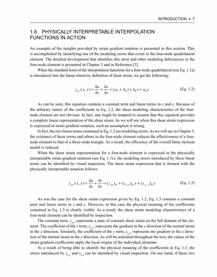
The defi ciency that exists with uniform refi nement will now be demonstrated by uniformly refi ning an example problem several times. The result of dividing each of the fi ve individual ele-ments contained in the initial model (see Fig. 1.2) into two elements is presented in Fig. 1.4a. When the strain distribution produced by the ten-element model is compared with the exact result, this uniformly refi ned model shows an improvement on the fi ve-element model, but it still does not accurately represent the maximum and minimum points of the exact solution. We will quantify these errors later when we develop error estimators. Note, however, that the interelement jumps at the critical points have been reduced in the refi ned model.

When the ten-element model is uniformly refi ned again, the model improves. As shown in Fig. 1.4b, the regions of the strain distribution with rapidly changing curvature before the minimum point and after the maximum point better represent the exact solution. Although the representations of the maximum and minimum points are improved, the fi nite element approximation of the strain distribution still does not give an accurate picture of the strain distribution in these regions. Note that a signifi cant interelement jump in the strain has appeared in the center of the bar where the strain is essentially zero.

0 1 2 3 4 5 6

–6

–4

–2

0

2

4

6

Elemental strains and exact strains vs. position

Location bar Location bar

Stra

in

10 elements

0 1 2 3 4 5 6–6

–4

–2

0

2

4

6

Elemental strains and exact strains vs. position

Stra

in

20 elements

(a) Ten-element strain results (b) Twenty-element strain results

Figure 1.4. Strain results for two successive uniform refi nements of Fig. 1.2.

10 • THE ESSENTIALS OF FINITE ELEMENT MODELING AND ADAPTIVE REFINEMENT

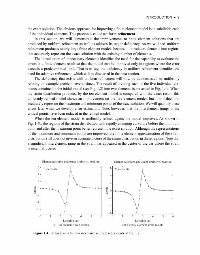
These two examples identify the diffi culties inherent in uniform refi nement. On one hand, ele-ments are added to regions that adequately represent the exact solution. On the other hand, not enough elements are added in regions of high error. These defi ciencies are further highlighted when the 20-element model is uniformly refi ned two more times as shown in Fig. 1.5.

0 1 2 3 4 5 6–5–4–3–2–1012345

Elemental strains and exact strains vs. position

Location bar Location bar

Stra

in

40 elements

0 1 2 3 4 5 6–5–4–3–2–1012345

Elemental strains and exact strains vs. position

(b) Eighty-element strain results

Stra

in

80 elements

(a) Forty-element strain results.

Figure 1.5. Strain results for two successive uniform refi nements of Fig. 1.4b.

As can be seen in Fig. 1.5a, the strain representation produced by this 40-element model is bet-ter than the approximation produced by the 20-element model. However, the region of maximum strain still does not match the exact solution well and the interelement jumps in the strain are clearly visible. When the fi nite element model is uniformly refi ned again as shown in Fig. 1.5b, the contour of the region of maximum error is captured reasonably well by the 80-element model. Note that the interelement jumps have been further reduced. They are primarily seen as a thickening of the circles that represent the interelement nodes.

The foregoing examples of uniform refi nements highlight the problem with uniform refi ne-ment. Too many elements are placed in regions where the actual strain distributions are adequately represented and not enough elements are placed in the critical regions with high rates of change in the strain distributions. An alternative approach that eliminates this defi ciency is outlined and demonstrated in the next section.

1.9 EXAMPLES OF ADAPTIVE REFINEMENT AND ERROR ANALYSIS

The initial fi nite element model of a problem rarely provides a solution that is accurate enough for use in the design process. The obvious strategy for improving the model is to repeatedly subdivide every element in the model until the change in two successive results is acceptably small. However,

INTRODUCTION • 11

as was seen in the previous section, this brute force approach for reaching an acceptable solution leads to fi nite element models that are unmanageably large because it needlessly introduces ele-ments into regions that contain little or no error.

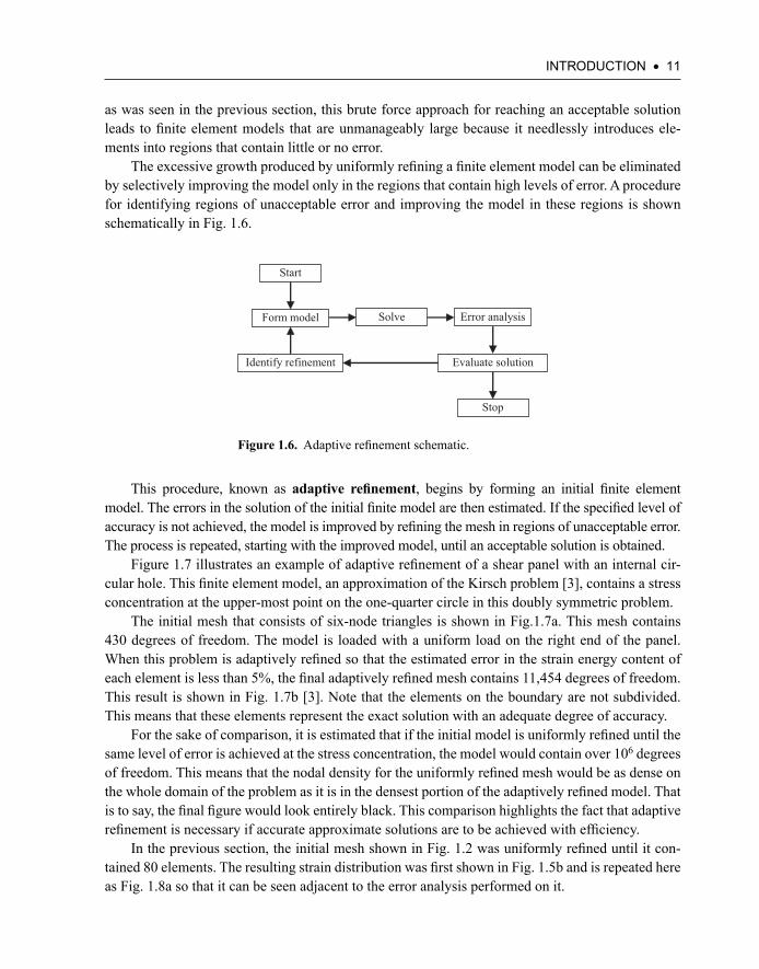
The excessive growth produced by uniformly refi ning a fi nite element model can be eliminated by selectively improving the model only in the regions that contain high levels of error. A procedure for identifying regions of unacceptable error and improving the model in these regions is shown schematically in Fig. 1.6.

Start

Form model Solve Error analysis

Identify refinement Evaluate solution

Stop

Figure 1.6. Adaptive refi nement schematic.

This procedure, known as adaptive refi nement, begins by forming an initial fi nite element model. The errors in the solution of the initial fi nite model are then estimated. If the specifi ed level of accuracy is not achieved, the model is improved by refi ning the mesh in regions of unacceptable error. The process is repeated, starting with the improved model, until an acceptable solution is obtained.

Figure 1.7 illustrates an example of adaptive refi nement of a shear panel with an internal cir-cular hole. This fi nite element model, an approximation of the Kirsch problem [3], contains a stress concentration at the upper-most point on the one-quarter circle in this doubly symmetric problem.

The initial mesh that consists of six-node triangles is shown in Fig.1.7a. This mesh contains 430 degrees of freedom. The model is loaded with a uniform load on the right end of the panel. When this problem is adaptively refi ned so that the estimated error in the strain energy content of each element is less than 5%, the fi nal adaptively refi ned mesh contains 11,454 degrees of freedom. This result is shown in Fig. 1.7b [3]. Note that the elements on the boundary are not subdivided. This means that these elements represent the exact solution with an adequate degree of accuracy.

For the sake of comparison, it is estimated that if the initial model is uniformly refi ned until the same level of error is achieved at the stress concentration, the model would contain over 106 degrees of freedom. This means that the nodal density for the uniformly refi ned mesh would be as dense on the whole domain of the problem as it is in the densest portion of the adaptively refi ned model. That is to say, the fi nal fi gure would look entirely black. This comparison highlights the fact that adaptive refi nement is necessary if accurate approximate solutions are to be achieved with effi ciency.

In the previous section, the initial mesh shown in Fig. 1.2 was uniformly refi ned until it con-tained 80 elements. The resulting strain distribution was fi rst shown in Fig. 1.5b and is repeated here as Fig. 1.8a so that it can be seen adjacent to the error analysis performed on it.

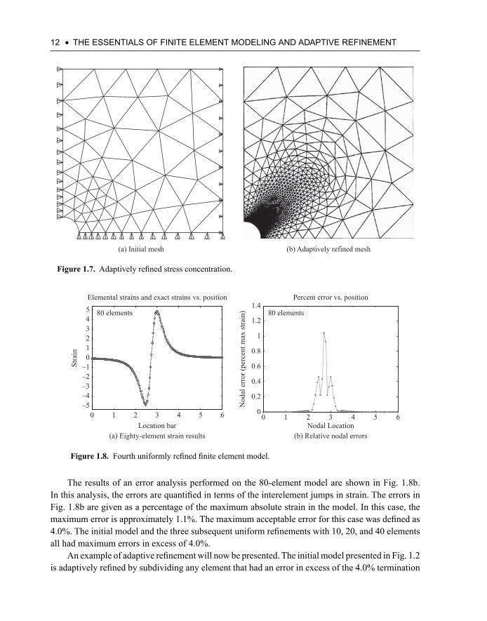
12 • THE ESSENTIALS OF FINITE ELEMENT MODELING AND ADAPTIVE REFINEMENT

The results of an error analysis performed on the 80-element model are shown in Fig. 1.8b. In this analysis, the errors are quantifi ed in terms of the interelement jumps in strain. The errors in Fig. 1.8b are given as a percentage of the maximum absolute strain in the model. In this case, the maximum error is approximately 1.1%. The maximum acceptable error for this case was defi ned as 4.0%. The initial model and the three subsequent uniform refi nements with 10, 20, and 40 elements all had maximum errors in excess of 4.0%.

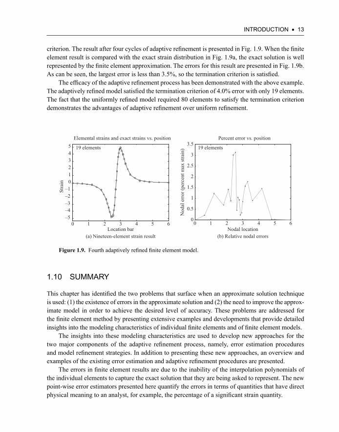
An example of adaptive refi nement will now be presented. The initial model presented in Fig. 1.2 is adaptively refi ned by subdividing any element that had an error in excess of the 4.0% termination

(a) Initial mesh (b) Adaptively refined mesh

Figure 1.7. Adaptively refi ned stress concentration.

Figure 1.8. Fourth uniformly refi ned fi nite element model.

0 1 2 3 4 5 6–5–4–3–2–1012345Elemental strains and exact strains vs. position

Location bar

Stra

in

80 elements

0 1 2 3 4 5 60

0.2

0.4

0.6

0.8

1

1.2

1.4Percent error vs. position

Nod

al e

rror

(per

cent

max

stra

in)

Nodal Location(a) Eighty-element strain results (b) Relative nodal errors

80 elements

INTRODUCTION • 13

criterion. The result after four cycles of adaptive refi nement is presented in Fig. 1.9. When the fi nite element result is compared with the exact strain distribution in Fig. 1.9a, the exact solution is well represented by the fi nite element approximation. The errors for this result are presented in Fig. 1.9b. As can be seen, the largest error is less than 3.5%, so the termination criterion is satisfi ed.

The effi cacy of the adaptive refi nement process has been demonstrated with the above example. The adaptively refi ned model satisfi ed the termination criterion of 4.0% error with only 19 elements. The fact that the uniformly refi ned model required 80 elements to satisfy the termination criterion demonstrates the advantages of adaptive refi nement over uniform refi nement.

Figure 1.9. Fourth adaptively refi ned fi nite element model.

0 1 2 3 4 5 6–5–4–3–2–1

012345

Elemental strains and exact strains vs. position

Location bar

Stra

in

19 elements

0 1 2 3 4 5 60

0.5

1

1.5

2

2.5

3

3.5Percent error vs. position

Nod

al e

rror

(per

cent

max

stra

in)

Nodal location(a) Nineteen-element strain result (b) Relative nodal errors

19 elements

1.10 SUMMARY

This chapter has identifi ed the two problems that surface when an approximate solution technique is used: (1) the existence of errors in the approximate solution and (2) the need to improve the approx-imate model in order to achieve the desired level of accuracy. These problems are addressed for the fi nite element method by presenting extensive examples and developments that provide detailed insights into the modeling characteristics of individual fi nite elements and of fi nite element models.

The insights into these modeling characteristics are used to develop new approaches for the two major components of the adaptive refi nement process, namely, error estimation procedures and model refi nement strategies. In addition to presenting these new approaches, an overview and examples of the existing error estimation and adaptive refi nement procedures are presented.

The errors in fi nite element results are due to the inability of the interpolation polynomials of the individual elements to capture the exact solution that they are being asked to represent. The new point-wise error estimators presented here quantify the errors in terms of quantities that have direct physical meaning to an analyst, for example, the percentage of a signifi cant strain quantity.

14 • THE ESSENTIALS OF FINITE ELEMENT MODELING AND ADAPTIVE REFINEMENT

The new approaches to mesh refi nement are based on the recognition that the fi nite element interpolation polynomials are actually truncated Taylor series expansions. This, in turn, allows the coeffi cients of the Taylor series expansions to be interpreted in terms of rigid body motions and strain quantities. The use of this physically interpretable, strain gradient notation allows the model-ing capacities of the individual elements to be compared with an estimation of the exact solution that is emerging from the fi nite element solution to identify model refi nements that lead to the rapid improvement of the fi nite element model.

1.11 REFERENCES

1. Scheid, F., Numerical Analysis, 2nd ed., McGraw-Hill, Inc, Schaum’s Outline Series, New York: McGraw-Hill Book Company, 1989, p. 267.This presentation of the Weierstrass approximation theorem is readily accessible to the non-mathematician.

2. Madson, J. C. and Handscomb, D. C., Chebyshev Polynomials, Boca Raton, FL: Chapman and Hall/CRC Press, 2003, p. 45.This is the fi rst new book on Chebyshev polynomials to be written in several decades. Its primary thesis is that much of numerical analysis can be based on Chebyshev polynomials.

3. Dow, J. O., A Unifi ed Approach to the Finite Element Method and Error Analysis Procedures, New York: Academic Press, 1999. This book puts the fi nite element method, the fi nite difference method, and error analysis on a common Taylor series basis. It develops and applies the physically based notation introduced in Chapter 3.

Also From Momentum Press

• Automotive Sensors by John Turner

• Biomedical Sensors by Deric P. Jones

• Centrifugal and Axial Compressor Control by Gregory K. McMillan

• Virtual Engineering by Joe Cecil,

• Reduce Your Engineering Drawing Errors: Preventing the Most Common Mistakes by Ronald Hanifan

• Bio-Inspired Engineering by Chris Jenkins

• Acoustic High-Frequency Diffraction Theory by Frederic Molinet

• 10 Volumes Edited by Ghenadii Korotcenkov on Chemical Sensors with details such as Fundamentals of Sensing Materials (Nanostructured Materials, General Approaches, and Polymers and Other Materials); Solid State Devices; Electrochemical and Optical Sensors; Chemical Sensors Applications; and Simulation and Modeling

Would You Like To Become an MP Author? Please Contact Joel Stein, joel@momentumpress.net

For more information, please visit www.momentumpress.net____________________________________________

Th e Momentum Press Digital Library45 Engineering Ebooks in One Digital Library or As Selected Topical Collections

Our ebrary platform, our digital collection features…

• a one-time purchase; not subscription based,• that is owned forever,• allows for simultaneous readers,• has no restrictions on printing, and• can be downloaded as a pdf

The Momentum Press digital library is an affordable way to give many readers simultaneous access

to expert content.

For more information, please visit www.momentumpress.net/library and to set up a trial, please contact adam.chesler@momentumpress.net.

ISBN: 978-1-60650-332-4

9 781606 503324

90000

www.momentumpress.net

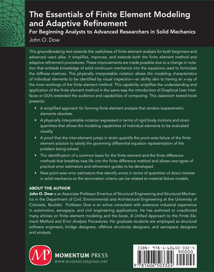
This groundbreaking text extends the usefulness of finite element analysis for both beginners and advanced users alike. It simplifies, improves, and extends both the finite element method and adaptive refinement procedures. These improvements are made possible due to a change in nota-tion that embeds knowledge of solid continuum mechanics into the equations used to formulate the stiffness matrices. This physically interpretable notation allows the modeling characteristics of individual elements to be identified by visual inspection—an ability akin to having an x-ray of the inner workings of the finite element method. This capability simplifies the understanding and application of the finite element method in the same way the introduction of Graphical User Inter-faces or GUI’s extended the audience and capabilities of computing. This classroom tested book presents:

elements obsolete.

quantities that allows the modeling capabilities of individual elements to be evaluated visually.

element solution to satisfy the governing differential equation representation of the problem being solved.

methods that breathes new life into the finite difference method and allows new types of practical error estimators and refinement guides to be developed.

in solid mechanics so the termination criteria can be related to material failure models.

ABOUT THE AUTHORJohn O. Dow -

in automotive, aerospace, and civil engineering applications. He has authored or coauthored many articles on finite element modeling and the book, A Unified Approach to the Finite Ele-ment Method and Error Analysis Procedures. His graduate students are employed as structural software engineers, bridge designers, offshore structures designers, and aerospace designers and analysts.

The Essentials of Finite Element Modeling and Adaptive RefinementFor Beginning Analysts to Advanced Researchers in Solid Mechanics

John O. Dow