The Establishment-Level Behavior of Vacancies and Hiring

30 December 2012

Steven J. Davis, University of Chicago, NBER and AEI* R. Jason Faberman, Federal Reserve Bank of Chicago

John C. Haltiwanger, University of Maryland and NBER

Abstract This paper is the first to study vacancies, hires, and vacancy yields at the establishment level in the Job Openings and Labor Turnover Survey, a large sample of U.S. employers. To interpret the data, we develop a simple model that identifies the flow of new vacancies and the job-filling rate for vacant positions. The fill rate moves counter to aggregate employment but rises steeply with employer growth rates in the cross section. It falls with employer size, rises with worker turnover rates, and varies by a factor of four across major industry groups. We also develop evidence that the employer-level hiring technology exhibits mild increasing returns in vacancies, and that employers rely heavily on other instruments, in addition to vacancies, as they vary hires. Building from our evidence and a generalized matching function, we construct a new index of recruiting intensity (per vacancy). Recruiting intensity partly explains the recent breakdown in the standard matching function, delivers a better-fitting empirical Beveridge Curve, and accounts for a large share of fluctuations in aggregate hires. Our evidence and analysis provide useful inputs for assessing, developing and calibrating theoretical models of search, matching and hiring in the labor market. Keywords: Vacancy yield, job-filling rate, hiring, labor market search, generalized matching function, recruiting intensity, returns to scale in vacancies, establishment data JEL Codes: D21, E24, J60 * Contact information: Steven.Davis@chicagobooth.edu, Jfaberman@.frbchi.org, Haltiwan@econ.umd.edu. We thank several anonymous referees, Peter Diamond, Shigeru Fujita, Larry Katz, Giuseppe Moscarini, Éva Nagypál, Josh Pinkston, Fabien Postel-Vinay, Mike Pries, Richard Rogerson, Rob Shimer and seminar participants at Berkeley, Chicago, LSE, Maryland, Michigan, Michigan State, National University of Singapore, Penn, Stanford, Bureau of Labor Statistics, the Federal Reserve Banks of Atlanta, Kansas City, New York, Philadelphia and San Francisco, and several conferences for many helpful comments. We thank Bruce Fallick, Charles Fleischman, and Rob Shimer for providing CPS data on gross worker flows and Marios Michaelides, Nathan Brownback, April Chen and Olga Deriy for excellent research assistance. Davis gratefully acknowledges financial support from the Booth School of Business. The views expressed are solely those of the authors and do not necessarily reflect the official positions or policies of the Federal Reserve Bank of Chicago, the Federal Reserve System, the U.S. Bureau of Labor Statistics, the U.S. Bureau of the Census or the views of other staff members.

1

I. INTRODUCTION

In many models of search, matching, and hiring in the labor market, employers post

vacancies to attract job seekers.1 These models often feature a matching function that

requires job seekers and job vacancies to produce new hires. The concept of a job vacancy

also plays an important role in mismatch and stock-flow matching models of the labor

market.2 Despite a key role in theoretical models, relatively few empirical studies consider

vacancies and their connection to hiring at the establishment level. Even at more aggregated

levels, our knowledge of vacancy behavior is very thin compared to our knowledge of

unemployment. As a result, much theorizing about vacancies and their role in the hiring

process takes place in a relative vacuum.

This study enriches our understanding of vacancy and hiring behavior and develops

new types of evidence for assessing, developing, and calibrating theoretical models. We

consider vacancy rates, new hires, and vacancy yields at the establishment level in the Job

Openings and Labor Turnover Survey (JOLTS), a large sample of U.S. employers. The

vacancy yield is the flow of realized hires during the month per reported job opening at the

end of the previous month. Using JOLTS data, we investigate how the hires rate, the

vacancy rate, and the vacancy yield vary with employer growth in the cross section, how

they differ by employer size, worker turnover, and industry, and how they move over time.

We first document some basic patterns in the data. The vacancy yield falls with

establishment size, rises with worker turnover, and varies by a factor of four across major

1 This description fits random search models such as Pissarides [1985] and Mortensen and Pissarides [1994], directed search models with wage posting such as Moen [1997] and Acemoglu and Shimer [2000], on-the-job search models such as Burdett and Mortensen [1998] and Nagypál [2007], and many others. The precise role of vacancies differs across these models. See Mortensen and Pissarides [1999], Rogerson, Shimer and Wright [2006] and Yashiv [2006] for reviews of research in this area. 2 See, for example, Hansen [1970] and Shimer [2007] for mismatch models and Coles and Smith [1998] and Ebrahimy and Shimer [2010] for stock-flow matching models.

2

industry groups. Employers with no recorded vacancies at month’s end account for 45% of

aggregate employment. At the same time, establishments reporting zero vacancies at

month’s end account for 42% of all hires in the following month.

The large share of hires by employers with no reported vacancy at least partly

reflects an unmeasured flow of new vacancies posted and filled within the month. This

unmeasured vacancy flow also inflates the measured vacancy yield. To address this and

other issues, we introduce a simple model of daily hiring dynamics. The model treats data

on the monthly flow of new hires and the stock of vacancies at month’s end as observed

outcomes of a daily process of vacancy posting and hiring. By cumulating the daily

processes to the monthly level, we can address the stock-flow distinction and uncover the

flow of new vacancies and the average daily job-filling rate during the month.

The job-filling rate is the employer counterpart to the much-studied job-finding rate

for unemployed workers.3 Although theoretical models of search and matching carry

implications for both job-finding and job-filling rates, the latter has received little attention.

Applying our model, we find that the job-filling rate moves counter-cyclically at the

aggregate level. In the cross section, vacancy durations are longer for larger establishments,

and job-filling rates are an order of magnitude greater at high compared to low turnover

establishments. Most striking, the job-filling rate rises very steeply with employer growth in

the cross section – from 1-2 percent per day at establishments with stable employment to

more than 10 percent per day for establishments that expand by 7% or more in the month.

Looking across industries, employer size classes, worker turnover groups, and

establishment growth rate bins, we find a recurring pattern: The job-filling rate exhibits a

3 Recent studies include Hall [2005a, 2005b], Shimer [2005, 2012], Yashiv [2007], Petrongolo and Pissarides [2008], Elsby, Michaels, and Solon [2009] and Fujita and Ramey [2009].

3

strong positive relationship to the gross hires rate. The same pattern emerges even more

strongly when we isolate changes over time at the establishment level. This pattern suggests

that employers rely heavily on other instruments, in addition to vacancies, as they vary the

rate of new hires. Other instruments – such as advertising expenditures, screening methods,

hiring standards, and compensation packages – influence job-filling rates through effects on

applications per vacancy, applicant screening times, and acceptance rates of job offers.

Another explanation for the positive relationship between job-filling rates and gross hires in

the micro data is increasing returns to vacancies in the employer-level hiring technology.

To evaluate these explanations and extend our analysis in other ways, we consider a

generalized matching function defined over unemployed workers, job vacancies, and

“recruiting intensity” per vacancy (shorthand for the effect of other instruments). As we

show, the corresponding hiring technology implies a tight relationship linking the hires

elasticity of job-filling rates in the micro data to employer-level scale economies in

vacancies and recruiting intensity per vacancy. Partly motivated by this relationship, we

devise an approach to estimating the degree of scale economies using JOLTS data. We find

evidence of mild increasing returns to vacancies in the employer-level hiring technology.

This novel result – interesting in its own right – allows us to recover the combined role of

other (non-vacancy) recruiting instruments in hiring outcomes from the empirical hires

elasticity of job-filling rates. Our evidence and analysis lead us to conclude that recruiting

intensity per vacancy drives the empirical hires elasticity of job-filling rates.

Our analysis and empirical investigation also yield new insights about aggregate

labor market fluctuations. Consider a standard CRS matching function defined over job

vacancies (v) and unemployed persons (u): , where µ > 0 and 0 < α < 1. The

4

implied vacancy yield is a decreasing function of labor market tightness, as measured by the

vacancy-unemployment ratio. Figure I plots this implied vacancy yield and shows that it

closely tracks the measured vacancy yield in JOLTS data from 2001 to 2007. 4 But the

relationship broke down in a major way in the next four years: Conditional on the number of

vacant jobs and unemployed workers, new hires are much lower from 2008 to 2011 than

implied by a standard matching function. This breakdown is a significant puzzle.

We provide a partial explanation and remedy for the breakdown, building from

micro evidence to quantify recruiting intensity per vacancy at the aggregate level. The

resulting generalized matching function outperforms the standard matching function in

several respects. First, as Figure I shows, incorporating a role for recruiting intensity

reduces the discrepancy between the measured vacancy yield and the empirical construct

implied by the matching function. Second, and closely related, our recruiting intensity

measure explains about one quarter of the aggregate time-series residuals produced by the

standard matching function, residuals that other authors interpret in terms of mismatch or

fluctuations in matching efficiency. Third, by generalizing the matching function to include

a role for recruiting intensity, we obtain a better-fitting empirical Beveridge Curve in

national and regional data. Finally, over the period covered by the JOLTS data, our

recruiting intensity index accounts for much of the movements in aggregate hires.5

4 The ratio of hires to vacancies is often treated as a measure of the job-filling rate. We reserve the latter term for the measure that adjusts for the stock-flow difference between the monthly flow of gross hires and the end-of-month vacancy stock in JOLTS data. As an empirical matter, the daily fill rate is nearly proportional to the vacancy yield in the aggregate time-series data. So we do not lose much by focusing on the vacancy yield in Figure I, and we gain simplicity. In the micro data, however, the near proportionality between vacancy yields and job-filling rates fails, and it becomes important to respect the stock-flow distinction. 5 In follow-on work, we develop additional evidence that the recruiting intensity concept and generalized matching function improve our understanding of aggregate labor market fluctuations. Davis, Faberman and Haltiwanger [2012] show that industry-level movements in job-filling rates are at odds with implications of the standard matching function but consistent with the implications of our generalized matching function. Davis

5

Our work also relates to several previous empirical studies of vacancy behavior. The

pioneering work of Abraham [1983, 1987] and Blanchard and Diamond [1989] uses the

Help Wanted Index (HWI) to proxy for vacancies, and many other studies follow their lead.

The Help Wanted Index yields sensible patterns at the aggregate level [Abraham 1987;

Blanchard and Diamond 1989; and Shimer, 2005], but it cannot accommodate an employer-

level analysis. Several recent studies exploit aggregate and industry-level JOLTS data on

hires, separations, and vacancies [Hall 2005a; Shimer 2005, 2007; Valetta 2005]. Earlier

studies by Holzer [1994], Burdett and Cunningham [1998] and Barron, Berger, and Black

[1999] consider vacancy behavior in small samples of U.S. employers. Van Ours and Ridder

[1991] investigate the cyclical behavior of vacancy flows and vacancy durations using

periodic surveys of Dutch employers. Coles and Smith [1996], Berman [1997], Yashiv

[2000], Dickerson [2003], Andrews et al. [2007] and Sunde [2007] exploit vacancy data

from centralized registers of job openings in various countries.

The next section describes our data and measurement mechanics. Section III

documents basic patterns in the behavior of vacancies and hires. Section IV sets forth our

model of daily hiring dynamics, fits it to the data, recovers the daily job-filling rate, and

develops evidence of how the fill rate varies over time and in the cross section. In Section V,

we interpret the evidence and extend the analysis in several ways. We introduce the

generalized matching function, and show how to extract information about the role of

recruiting intensity and scale economies in the hiring process. We then turn to aggregate

implications and relate our evidence to leading search models. Section VI concludes with a

summary of our main contributions and some remarks about directions for future research.

[2011] shows that using our recruiting intensity index in a generalized matching function helps to explain the plunge in job-finding rates during the Great Recession and their failure to recover afterwards.

6

II. DATA SOURCES AND MEASUREMENT MECHANICS

The Job Openings and Labor Turnover Survey (JOLTS) samples about 16,000

establishments per month. Respondents report hires and separations during the month,

employment in the pay period covering the 12th of the month, and job openings at month’s

end. JOLTS data commence in December 2000, and our establishment-level sample

continues through December 2006. We drop observations that are not part of a sequence of

two or more consecutive observations for the same establishment. This restriction enables a

comparison of hires in the current month to vacancies at the end of the previous month, an

essential element of our micro-based analysis. The resulting sample contains 577,268

observations, about 93% of the full sample that the BLS uses for published JOLTS statistics.

We have verified that this sample restriction has little effect on aggregate estimates of

vacancies, hires, and separations.6 While our JOLTS micro data set ends in December 2006,

we consider the period through December 2011 for analyses that use published JOLTS data.

It will be helpful to describe how job openings (vacancies) are defined and measured

in JOLTS. The survey form instructs the respondent to report a vacancy when “a specific

position exists, work could start within 30 days, and [the establishment is] actively seeking

workers from outside this location to fill the position.” The respondent is asked to report the

number of such vacancies on “the last business day of the month.” Further instructions

define “active recruiting” as “taking steps to fill a position. It may include advertising in

newspapers, on television, or on radio; posting Internet notices; posting ‘help wanted’ signs;

networking or making ‘word of mouth’ announcements; accepting applications;

6 There is a broader selection issue in that the JOLTS misses most establishment births and deaths, which may be why our sample restriction has little impact on aggregate estimates. Another issue is the potential impact of JOLTS imputations for item nonresponse, on which we rely. See Clark and Hyson [2001], Clark [2004] and Faberman [2008] for detailed discussions of JOLTS. See Davis, Faberman, Haltiwanger, and Rucker [2010] for an analysis of how the JOLTS sample design affects the published JOLTS statistics.

7

interviewing candidates; contacting employment agencies; or soliciting employees at job

fairs, state or local employment offices, or similar sources.” Vacancies are not to include

positions open only to internal transfers, promotions, recalls from temporary layoffs, jobs

that commence more than 30 days hence, or positions to be filled by temporary help

agencies, outside contractors, or consultants.

Turning to measurement mechanics, we calculate an establishment’s net employment

change in month t as its reported hires in month t minus its reported separations in . We

subtract this net change from its reported employment in t to obtain employment in 1.

This method ensures that the hires, separations, and employment measures in the current

month are consistent with employment for the previous month. To express hires,

separations, and employment changes at t as rates, we divide by the simple average of

employment in 1 and . The resulting growth rate measure is bounded, symmetric about

zero and has other desirable properties, as discussed in Davis, Haltiwanger, and Schuh

[1996]. We measure the vacancy rate at t as the number of vacancies reported at the end of

month t divided by the sum of vacancies and the simple average of employment in 1 and

. The vacancy yield in is the number of hires reported in divided by the number of

vacancies reported at the end of 1.

III. SECTORAL AND ESTABLISHMENT-LEVEL PATTERNS

III.A. Cross-Sectional Patterns

Table I draws on JOLTS micro data to report the hires rate, separation rate, vacancy

rate, and vacancy yield by industry, employer size group, and worker turnover group.

Worker turnover is measured as the sum of the monthly hires and separations rates at the

establishment. All four measures show considerable cross-sectional variation, but we focus

8

our remarks on the vacancy yield. Government, Health & Education, Information and FIRE

have low vacancy yields on the order of 0.8 hires during the month per vacancy at the end of

the previous month. Construction, an outlier in the other direction, has a vacancy yield of

3.1. The vacancy yield falls by more than half in moving from establishments with fewer

than 50 employees to those with more than 1,000. It rises by a factor of ten in moving from

the bottom to the top turnover quintile.

What explains these strong cross-sectional patterns? One possibility is that matching

is intrinsically easier in certain types of jobs. For example, Albrecht and Vroman [2002]

build a matching model with heterogeneity in worker skill levels and in skill requirements of

jobs. Jobs with greater skill requirements have longer expected vacancy durations because

employers are choosier about whom to hire. Barron, Berger, and Black [1999] provide

evidence that search efforts and vacancy durations depend on skill requirements. Davis

[2001] identifies a different effect that leads to shorter durations in better jobs. In his model,

employers with more productive jobs search more intensively because the opportunity cost

of a vacancy is greater. Thus, if all employers use the same search and matching technology,

more productive jobs fill at a faster rate. Yet another possibility is that workers and

employers sort into separate search markets, each characterized by different tightness,

different matching technologies, or both. Given the standard matching function described in

the introduction, this type of heterogeneity gives rise to differences in vacancy yields across

labor markets defined by observable and relevant employer characteristics.

Another explanation recognizes that firms recruit, screen, and hire workers through a

variety of channels, and that reliance on these channels differs across industries and

employers. For example, construction firms may recruit workers from a hiring hall or other

9

specialized labor pool for repeated short-term work, perhaps reducing the incidence of

measured vacancies and inflating the vacancy yield. In contrast, government and certain

other employers operate under laws and regulations that require a formal search process for

the vast majority of new hires, ensuring that most hiring is mediated through measured

vacancies. More generally, employers rely on a mix of recruiting and hiring practices that

differ in propensity to involve a measured vacancy and in vacancy duration. These methods

include bulk screening of applicants who respond to help-wanted advertisements, informal

recruiting through social networks, opportunistic hiring of attractive candidates, impromptu

hiring of unskilled workers in spot labor markets, and the conversion of temp workers and

independent contractors into permanent employees. Differences in the mix of recruiting,

screening and hiring practices lead to cross-sectional differences in the vacancy yield.

III.B. The Establishment-Level Distribution of Vacancies and Hires

Table II and Figure II document the large percentage of employers with few or no

reported vacancies. In the average month, 45% of employment is at establishments with no

reported vacancies. The employment-weighted median vacancy rate is less than 1% of

employment, calculated in an employment-weighted manner, and the median number of

vacancies is just one. At the 90th percentile of the employment-weighted distribution, the

vacancy rate is 6% of employment and the number of vacancies is 63. Weighting all

establishments equally, 88 percent report no vacancies, the vacancy rate at the 90th percentile

is 3%, and the number of vacancies at the 90th percentile is just one. The establishment-

level incidence of vacancies is highly persistent: only 18% of vacancies in the current month

occur at establishments with no recorded vacancies in the previous month.

10

Establishments with zero hires during the month account for 35% of employment,

which suggests that many employers have little need for hires at the monthly frequency.

However, Table II also reports that 42% of hires take place at establishments with no

reported vacancy going into the month. This fact suggests that average vacancy durations

are very short, or that much hiring is not mediated through vacancies as the concept is

defined and measured in JOLTS. We return to this issue in Section IV.

III.C. Hires, Vacancies, and Establishment Growth

We next consider how hires, vacancies, and vacancy yields co-vary with employer

growth rates at the establishment level. To estimate these relationships in a flexible

nonparametric manner, proceed as follows. First, partition the feasible range of growth rates,

[-2.0, 2.0], into 195 non-overlapping intervals, or bins, allowing for mass points at -2, 0 and

2. We use very narrow intervals of width .001 near zero and wider intervals in thinner parts

of the distribution. Next, sort the 577,000 establishment-level observations into bins based

on monthly employment growth rates, and calculate employment-weighted means for the

hires rate, the vacancy rate, and the vacancy yield for each bin. Equivalently, we perform an

OLS regression of the outcome variables on an exhaustive set of bin dummies. The

regression coefficients on the bin dummies recover the nonparametric relationship of the

outcome variables to the establishment-level growth rate of employment. Under the

regression approach, it is easy to introduce establishment fixed effects or other controls.

Figures III, IV, and V display the nonparametric regression results.7 The hires

relation must satisfy part of an adding-up constraint, because net growth is the difference

between hires and separations. Thus, the minimum feasible value for the hires rate lies along 7 We focus on monthly growth rate intervals in the -30 to 30% range because our estimates are highly precise in this range. For visual clarity, we smooth the nonparametric estimates using a centered, five-bin moving average except for bins at and near zero, where we use no smoothing.

11

the horizontal axis for negative growth and along the 45-degree line for positive growth.

Hiring exceeds this minimum at all growth rates, more so as growth increases.

Figure III shows a highly nonlinear, kinked relationship between the hires rate and

the establishment growth rate. The hires rate declines only slightly with employment growth

at shrinking establishments, reaching its minimum for establishments with no employment

change. To the right of zero, the hire rate rises slightly more than one-for-one with the

growth rate of employment. This cross-sectional relationship says that hires and job

creation are very tightly linked at the establishment level. Controlling for establishment

fixed effects in the regression, and thereby isolating within-establishment time variation,

does little to alter the relationship. In fact, the “hockey-stick” shape of the hires-growth

relation is even more pronounced when we control for establishment fixed effects.

Figure IV reveals a qualitatively similar relationship for the vacancy rate. Vacancy

rates average about 2% of employment at contracting establishments, dip for stable

establishments with no employment change, and rise with the employment growth rate at

expanding establishments. The vacancy-growth relationship for expanding establishments is

much less steep than the hires-growth relationship. For example, at a 30% monthly growth

rate, the vacancy rate is 4.8% of employment compared to 34.2% for the hires rate.

Figure V presents the vacancy yield relationship. We report total hires divided by

total vacancies in each bin, which is similar to dividing the hires relation in Figure III by the

vacancy relation in Figure IV.8 Among contracting establishments, vacancies yield about

one hire per month. There is a discontinuity at zero that vanishes when controlling for

8 It is not identical because the hires and vacancy rates have different denominators. Another alternative is to construct the vacancy yield at the establishment level and then aggregate to the bin level by computing employment-weighted means. This alternative, which restricts the sample to establishments with vacancies, yields a pattern very similar to the one reported in Figure V.

12

establishment fixed effects. Among expanding establishments, the vacancy yield increases

markedly with the growth rate. The strongly increasing relation between vacancy yields and

employer growth survives the inclusion of establishment fixed effects.9 In other words,

employers hire more workers per recorded vacancy when they grow more rapidly.

Taken at face value, this finding is starkly at odds with the proposition that

(expected) hires are proportional to vacancies. This proposition holds in the textbook search

and matching model and most other models with undirected search, as we discuss below. It

is unclear, however, whether this finding accurately portrays the underlying economic

relationship. It may instead reflect a greater unobserved flow of new vacancies filled during

the month at more rapidly growing establishments. The basic point is that, because of time

aggregation, we cannot confidently infer the economic relationship between vacancies and

hires from raw JOLTS data. We address this concern in the next section.

IV. JOB-FILLING RATES AND VACANCY FLOWS

IV.A. A Model of Daily Hiring Dynamics

Consider a simple model of daily hiring dynamics where hs,t is the number of hires

on day s in month t, and vs,t is the number of vacancies. Denote the daily job-filling rate for

vacant positions in month t by ft, which we treat as constant within the month for any given

establishment. Hires on day s in month t equal the fill rate times the vacancy stock:

(1) .

9 We regress the hiring (and vacancy) rates on bin dummies and establishment fixed effects, recovering the coefficients on the bin dummies and adding an equal amount to each coefficient to restore the grand employment-weighted mean. We then take the ratio of resulting hiring and vacancy rates to obtain the curve in Figure V with controls for establishment fixed effects. Restricting the sample to establishments with vacancies and running the fixed effects regression directly on the ratio of hires to vacancies yields a very similar plot.

tstts vfh ,1,

13

The stock of vacancies evolves in three ways. First, a daily flow of new vacancies

increases the stock. Second, hires deplete the stock. Third, vacancies lapse without being

filled at the daily rate also depleting the stock. These assumptions imply the daily law

of motion for the vacancy stock during month t:

(2) .

In fitting the model to data, we allow to vary with industry, establishment size

and other observable employer characteristics.

Next, sum equations (1) and (2) over workdays to obtain monthly measures that

correspond to observables in the data. For vacancies, relate the stock at the end of month

t – 1, vt-1, to the stock at the end of month t, days later. Cumulating (2) over days and

recursively substituting for vs-1,t yields the desired equation:

(3) .

The first term on the right is the initial stock, depleted by hires and lapsed vacancies during

the month. The second term is the flow of new vacancies, similarly depleted.

Hires are reported as a monthly flow in the data. Thus, we cumulate daily hires in

(1) to obtain the monthly flow, . Substituting (2) into (1), and (1) into the

monthly sum, and then substituting back to the beginning of the month for vs-1,t yields

(4) .

The first term on the right is hires into the old stock of vacant positions, and the second is

hires into positions that open during the month. Given the system (3)

and (4) identifies the average daily job-filling rate, ft, and the daily flow of vacancies, t.

t

t ,

ttsttts vfv ,1, ))1)(1((

ft , t and t

1

11 )1()1(

s

sttttttttttt ffvffv

1,

stst hH

1

1

1

11 )1)(()1(

s

stttttt

s

sttttttt ffsfffvfH

Ht , vt , vt1, and t ,

14

IV.B. Estimating the Model Parameters

To estimate , we solve the system (3) and (4) numerically after first

equating to the monthly layoff rate. That is, we assume vacant job positions lapse at the

same rate as filled jobs undergo layoffs. The precise treatment of matters little for our

results because any reasonable value for is an order of magnitude smaller than the

estimates for Thus the job-filling rate dominates the behavior of the dynamic system

given by (1) and (2). We treat all months as having = 26 working days, the average

number of days per month less Sundays and major holidays. We calculate the average

vacancy duration as and express the monthly vacancy flow as a rate by dividing by

employment in month t.10

When estimating parameters at the aggregate level, we use published JOLTS

statistics for monthly flows of hires and layoffs and the end-of-month stock of vacancies.

We use the pooled-sample JOLTS micro data from 2001 to 2006 to produce parameter

estimates by industry, size class, turnover category, and growth rate bin.

IV.C. Fill Rates and Vacancy Flows over Time

Figure VI shows monthly time series from January 2001 to December 2011 for the

estimated flow of new vacancies and the daily job-filling rate. The monthly flow of new

vacancies averages 3.6% of employment, considerably larger than the average vacancy stock

of 2.7%. Vacancy stocks and flows are pro-cyclical, with stronger movements in the stock

10 We also tried an estimation approach suggested by Rob Shimer. The approach considers steady-state versions of (1) and (2) and sums over workdays to obtain ⁄ 1⁄ and . This system is simple enough to solve by hand. In practice, the method works well on aggregate data, delivering estimates for and close to the ones implied by (3) and (4). At more disaggregated levels, estimates based on the steady-state approximation often diverge from those implied by (3) and (4), sometimes greatly. Note that the estimated job-filling rate based on the steady-state approximation is simply a rescaled version of the vacancy yield. We stick to the method based on (3) and (4) for our reported results.

ft and t

t

f .

1 / ft t

15

measure. The average daily job-filling rate is 5.2% per day. It ranges from a low of 4.0% in

February 2001 to a high of 6.9% in July 2009, moving counter cyclically. Mean vacancy

duration ranges from 14 to 25 days.11 Clearly, vacancy durations and job-filling rates

exhibit large cyclical amplitudes. 12

IV.D. Results by Industry, Employer Size and Worker Turnover

Table III presents cross-sectional results based on the pooled-sample JOLTS micro

data from 2001 to 2006. The job-filling rate ranges from about 3% per day in Information,

FIRE, Health & Education and Government to 5% in Manufacturing, Transport, Wholesale

& Utilities, Professional & Business Services and Other Services, 7% in Retail Trade and

Natural Resources & Mining and 12% per day in Construction. Table III also shows that

job-filling rates decline with employer size, falling by more than half in moving from small

to large establishments. The most striking pattern in the job-filling rate pertains to worker

turnover categories. The job-filling rate ranges from 1.1% per day in the lowest turnover

quintile to 11.4% per day in the highest turnover quintile. These cross-sectional differences

have received little attention in the theoretical literature, but they offer a natural source of

inspiration for model building and a useful testing ground for theory.13

IV.E. Vacancy Flows and Fill Rates Related to Establishment Growth Rates

Section III finds that the vacancy yield increases strongly with the employment

growth rate at expanding establishments. As we explained, this relationship is at least partly

11 Our vacancy duration estimates are similar to those obtained by Burdett and Cunningham [1998] and Barron, Berger, and Black [1999] in small samples of U.S establishments but considerably shorter than those obtained by van Ours and Ridder [1991] for the Netherlands and Andrews et al. [2007] for the U.K. 12Figures B.1-B.3 in Online Appendix B applies our methods to data on new hires from the Current Population Survey and the Conference Board’s Help Wanted Index to provide additional evidence on the cyclicality of job-filling rates. 13 To be sure, there has been some theoretical work that speaks to cross-sectional differences in job-filling rates, including the works by Albrecht and Vroman [2002] and Davis [2001] mentioned above.

16

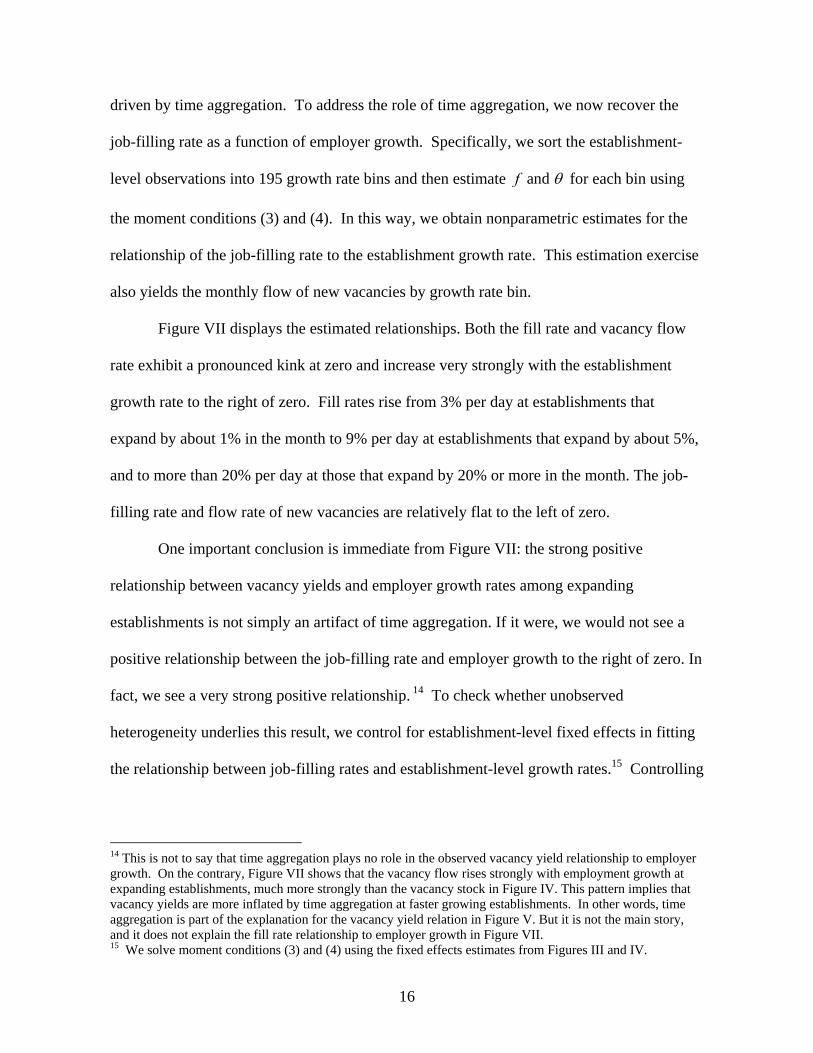
driven by time aggregation. To address the role of time aggregation, we now recover the

job-filling rate as a function of employer growth. Specifically, we sort the establishment-

level observations into 195 growth rate bins and then estimate for each bin using

the moment conditions (3) and (4). In this way, we obtain nonparametric estimates for the

relationship of the job-filling rate to the establishment growth rate. This estimation exercise

also yields the monthly flow of new vacancies by growth rate bin.

Figure VII displays the estimated relationships. Both the fill rate and vacancy flow

rate exhibit a pronounced kink at zero and increase very strongly with the establishment

growth rate to the right of zero. Fill rates rise from 3% per day at establishments that

expand by about 1% in the month to 9% per day at establishments that expand by about 5%,

and to more than 20% per day at those that expand by 20% or more in the month. The job-

filling rate and flow rate of new vacancies are relatively flat to the left of zero.

One important conclusion is immediate from Figure VII: the strong positive

relationship between vacancy yields and employer growth rates among expanding

establishments is not simply an artifact of time aggregation. If it were, we would not see a

positive relationship between the job-filling rate and employer growth to the right of zero. In

fact, we see a very strong positive relationship. 14 To check whether unobserved

heterogeneity underlies this result, we control for establishment-level fixed effects in fitting

the relationship between job-filling rates and establishment-level growth rates.15 Controlling

14 This is not to say that time aggregation plays no role in the observed vacancy yield relationship to employer growth. On the contrary, Figure VII shows that the vacancy flow rises strongly with employment growth at expanding establishments, much more strongly than the vacancy stock in Figure IV. This pattern implies that vacancy yields are more inflated by time aggregation at faster growing establishments. In other words, time aggregation is part of the explanation for the vacancy yield relation in Figure V. But it is not the main story, and it does not explain the fill rate relationship to employer growth in Figure VII. 15 We solve moment conditions (3) and (4) using the fixed effects estimates from Figures III and IV.

f and

17

for heterogeneity actually strengthens the relationship between the job-filling rate and the

growth rate of employment. Removing time effects (not shown) has negligible impact.

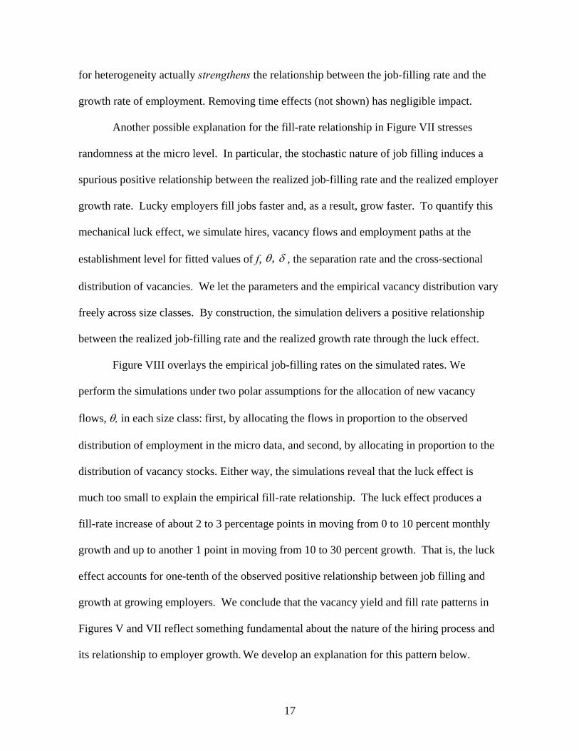
Another possible explanation for the fill-rate relationship in Figure VII stresses

randomness at the micro level. In particular, the stochastic nature of job filling induces a

spurious positive relationship between the realized job-filling rate and the realized employer

growth rate. Lucky employers fill jobs faster and, as a result, grow faster. To quantify this

mechanical luck effect, we simulate hires, vacancy flows and employment paths at the

establishment level for fitted values of f, , the separation rate and the cross-sectional

distribution of vacancies. We let the parameters and the empirical vacancy distribution vary

freely across size classes. By construction, the simulation delivers a positive relationship

between the realized job-filling rate and the realized growth rate through the luck effect.

Figure VIII overlays the empirical job-filling rates on the simulated rates. We

perform the simulations under two polar assumptions for the allocation of new vacancy

flows, , in each size class: first, by allocating the flows in proportion to the observed

distribution of employment in the micro data, and second, by allocating in proportion to the

distribution of vacancy stocks. Either way, the simulations reveal that the luck effect is

much too small to explain the empirical fill-rate relationship. The luck effect produces a

fill-rate increase of about 2 to 3 percentage points in moving from 0 to 10 percent monthly

growth and up to another 1 point in moving from 10 to 30 percent growth. That is, the luck

effect accounts for one-tenth of the observed positive relationship between job filling and

growth at growing employers. We conclude that the vacancy yield and fill rate patterns in

Figures V and VII reflect something fundamental about the nature of the hiring process and

its relationship to employer growth. We develop an explanation for this pattern below.

,

18

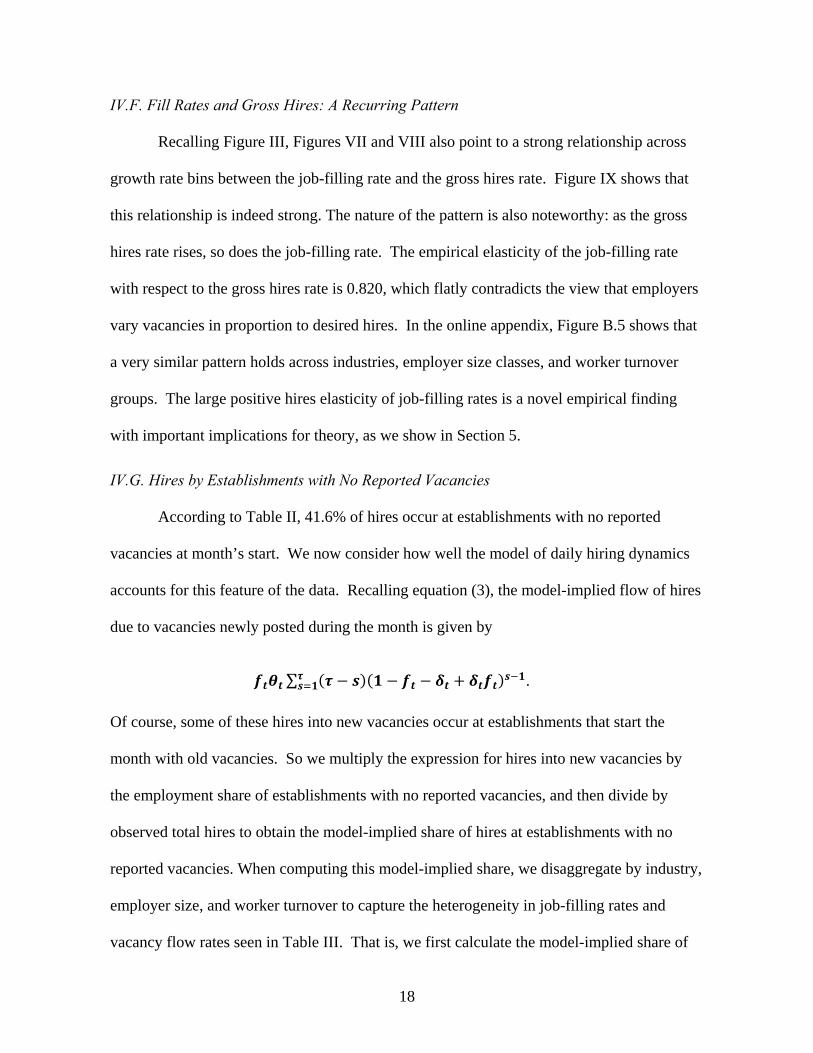
IV.F. Fill Rates and Gross Hires: A Recurring Pattern

Recalling Figure III, Figures VII and VIII also point to a strong relationship across

growth rate bins between the job-filling rate and the gross hires rate. Figure IX shows that

this relationship is indeed strong. The nature of the pattern is also noteworthy: as the gross

hires rate rises, so does the job-filling rate. The empirical elasticity of the job-filling rate

with respect to the gross hires rate is 0.820, which flatly contradicts the view that employers

vary vacancies in proportion to desired hires. In the online appendix, Figure B.5 shows that

a very similar pattern holds across industries, employer size classes, and worker turnover

groups. The large positive hires elasticity of job-filling rates is a novel empirical finding

with important implications for theory, as we show in Section 5.

IV.G. Hires by Establishments with No Reported Vacancies

According to Table II, 41.6% of hires occur at establishments with no reported

vacancies at month’s start. We now consider how well the model of daily hiring dynamics

accounts for this feature of the data. Recalling equation (3), the model-implied flow of hires

due to vacancies newly posted during the month is given by

∑ .

Of course, some of these hires into new vacancies occur at establishments that start the

month with old vacancies. So we multiply the expression for hires into new vacancies by

the employment share of establishments with no reported vacancies, and then divide by

observed total hires to obtain the model-implied share of hires at establishments with no

reported vacancies. When computing this model-implied share, we disaggregate by industry,

employer size, and worker turnover to capture the heterogeneity in job-filling rates and

vacancy flow rates seen in Table III. That is, we first calculate the model-implied share of

19

hires at establishments with no reported vacancies by sector and then compute the hires-

weighted mean over sectors, which we compare to the 41.6% figure.

Table IV reports the results of the comparison. When we slice the data by 6

employer size categories crossed with (up to) 15 worker turnover categories and a broad

division into goods-producing and service-producing industries, our model of daily hiring

dynamics implies that 27.4% of all hires occur at establishments with no recorded vacancies.

This quantity is about two-thirds of the 41.6% figure observed directly in the data. The

other classifications reported in Table IV produce somewhat smaller figures for hires at

establishments with no reported vacancies. We do not consider finer classifications because

of concerns about sparsely populated cells and imprecise cell-level estimates of f and .

Table IV tells us that time aggregation accounts for most, but by no means all, hires

at establishments with no reported vacancies. The unexplained hires may reflect a failure to

adequately capture cross-sectional heterogeneity in f and or some other form of model

misspecification. Perhaps the most natural interpretation, however, is that many hires are

not mediated through measured vacancies. For example, JOLTS definitions exclude

vacancies for positions that could not begin within 30 days. Certain other hires are unlikely

to be captured by the JOLTS vacancy measure, because they involve hires into positions

with zero prior vacancy duration. Using data on job applications and hires in the 1982 wave

of the Employment Opportunity Pilot Project Survey, Faberman and Menzio [2010] report

that 20% of all new hires involve no formal vacancy or recruiting time by the employer.

Based on Table IV and our discussion here, we think the topic of hires not mediated through

vacancies warrants attention in future research and in surveys of hiring practices.

20

V. INTERPRETATIONS AND IMPLICATIONS

V.A. Hires Are Not Proportional to Vacancies in the Cross Section: Two Interpretations

Standard specifications of equilibrium search and matching models include a

constant-returns-to-scale (CRS) matching function defined over job vacancies and

unemployed workers. In versions of these models taken to data, the number of vacancies is

typically the sole instrument employers use to vary hires. The expected period-t hires for an

employer e with vacancies are where the fill-rate is determined by market

tightness at t and the matching function, both exogenous to the employer. That is, hires are

proportional to vacancies in the cross section, i.e., conditional on market tightness.16 Since

the same fill rate applies to all employers, the standard specification implies a zero cross-

sectional elasticity of hires (and the hires rate) with respect to the fill rate. This implication

fails – rather spectacularly – when set against the evidence in Figures VII, VIII and IX.17

What accounts for this failure? One possibility is that employers act on other

margins using other instruments, in addition to vacancies, when they increase their hiring

rate. They can increase advertising or search intensity per vacancy, screen applicants more

quickly, relax hiring standards, improve working conditions, and offer more attractive

compensation to prospective employees. If employers with greater hiring needs respond in

this way, the job-filling rate rises with the hires rate in the cross section and over time at the

employer level. We are not aware of previous empirical studies that investigate how these

aspects of recruiting intensity per vacancy vary with employer growth and hiring. 16 To see the connection to our model of daily hiring dynamics, recall from footnote 10 that steady-state approximations of (1) and (2) yield . 17 Online Appendix A makes this point in a different way. Using the daily model of hiring dynamics, we express log gross hires as the sum of two terms – one that depends only on the job-filling rate, and one that depends on the numbers of old and new vacancies. Computing the implied variance decomposition, the vacancy margin accounts for half or less of the variance in log gross hires across industries, size classes, turnover groups, and growth rate bins. The proportionality implication says that vacancy numbers are all that matter for cross-sectional hires variation, sharply at odds with the variance decomposition results.

vet ftvet , ft

21

Another class of explanations involves scale and scope economies in vacancies as an

input to hiring. It may be easier or less costly to achieve a given advertising exposure per

job opening when an employer has many vacancies rather than few. Similarly, it may be

easier to attract applicants when the employer has a variety of open positions. Recruiting

also becomes easier as an employer grows more rapidly if prospective hires perceive greater

opportunities for promotion and lower layoff risks. These remarks point to potential sources

of increasing returns to vacancies in the employer-level hiring technology.

Alternatively, one might try to rationalize the evidence by postulating suitable cross-

sectional differences in matching efficiency. We think an explanation along those lines is

unsatisfactory in two significant respects. First, it offers no insight into why matching

efficiency varies across sectors in line with the gross hires rate. Second, sectoral differences

in matching efficiency do not explain the key result in Figure VII (Figure IX): The job-

filling rate is much higher when a given establishment grows (hires) rapidly, relative to its

own sample mean growth (hires) rate, than when it grows (hires) slowly. A stable CRS

hiring technology at the establishment level cannot produce this pattern when vacancies are

the sole instrument employers vary to influence hiring.

V.B. Generalized Matching and Hiring Functions

It will be useful to formalize a role for other recruiting instruments and for employer-

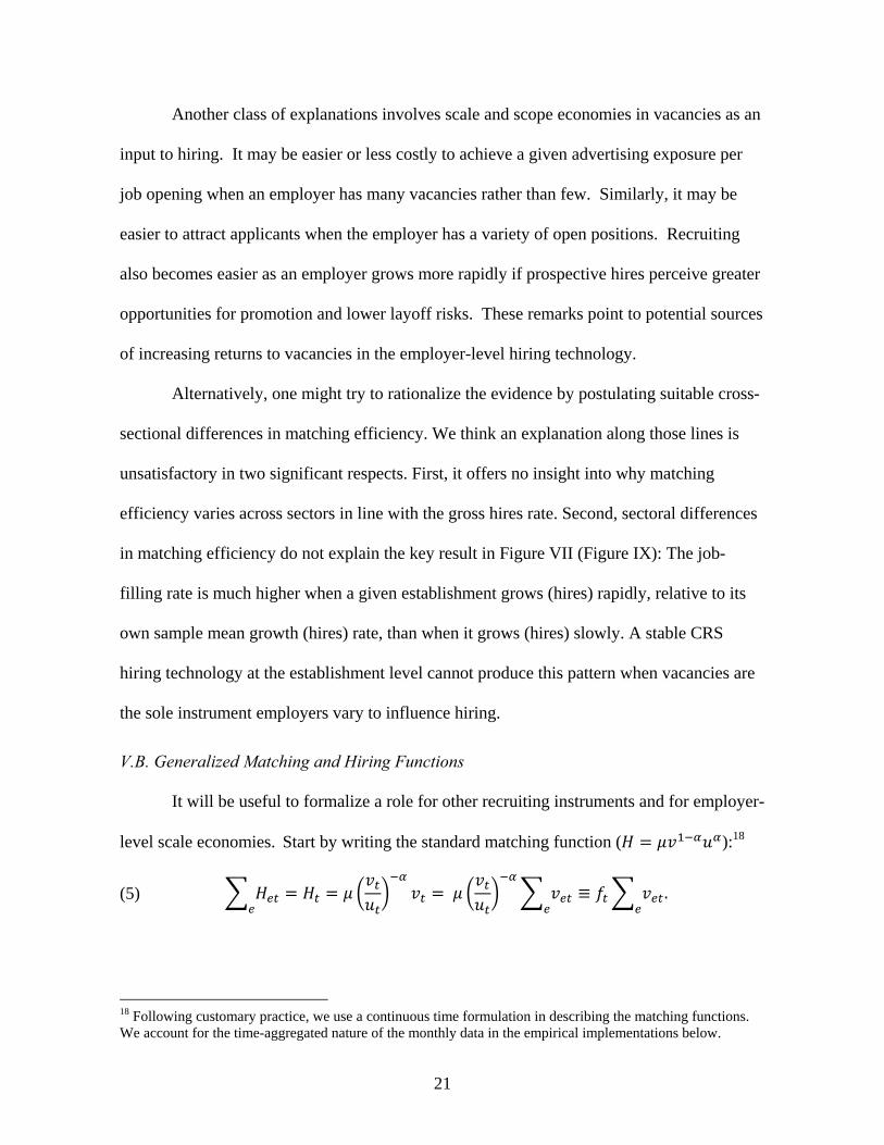
level scale economies. Start by writing the standard matching function ( ):18

(5) ≡ .

18 Following customary practice, we use a continuous time formulation in describing the matching functions. We account for the time-aggregated nature of the monthly data in the empirical implementations below.

22

For an individual employer or group of employers, e, (5) implies hires . Here

and throughout the discussion below, we ignore the distinction between hires and expected

hires by appealing to the law of large numbers when e indexes industries, size classes or

worker turnover groups. The simulation exercises reported in Figure VIII indicate that we

can safely ignore the distinction for growth rate bins as well.

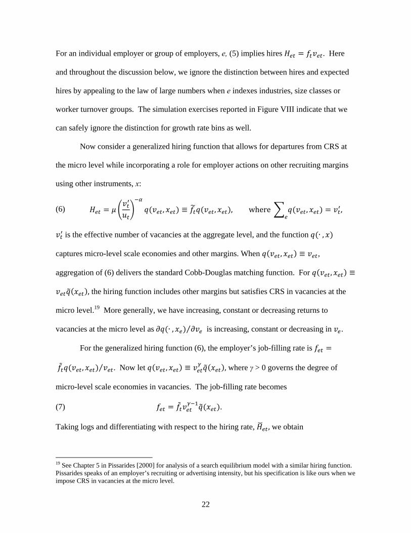
Now consider a generalized hiring function that allows for departures from CRS at

the micro level while incorporating a role for employer actions on other recruiting margins

using other instruments, x:

(6) , ≡ , , where , ,

is the effective number of vacancies at the aggregate level, and the function ∙,

captures micro-level scale economies and other margins. When , ≡ ,

aggregation of (6) delivers the standard Cobb-Douglas matching function. For , ≡

, the hiring function includes other margins but satisfies CRS in vacancies at the

micro level.19 More generally, we have increasing, constant or decreasing returns to

vacancies at the micro level as ∙, ⁄ is increasing, constant or decreasing in .

For the generalized hiring function (6), the employer’s job-filling rate is

, ⁄ . Now let , ≡ , where γ > 0 governs the degree of

micro-level scale economies in vacancies. The job-filling rate becomes

(7) .

Taking logs and differentiating with respect to the hiring rate, , we obtain

19 See Chapter 5 in Pissarides [2000] for analysis of a search equilibrium model with a similar hiring function. Pissarides speaks of an employer’s recruiting or advertising intensity, but his specification is like ours when we impose CRS in vacancies at the micro level.

23

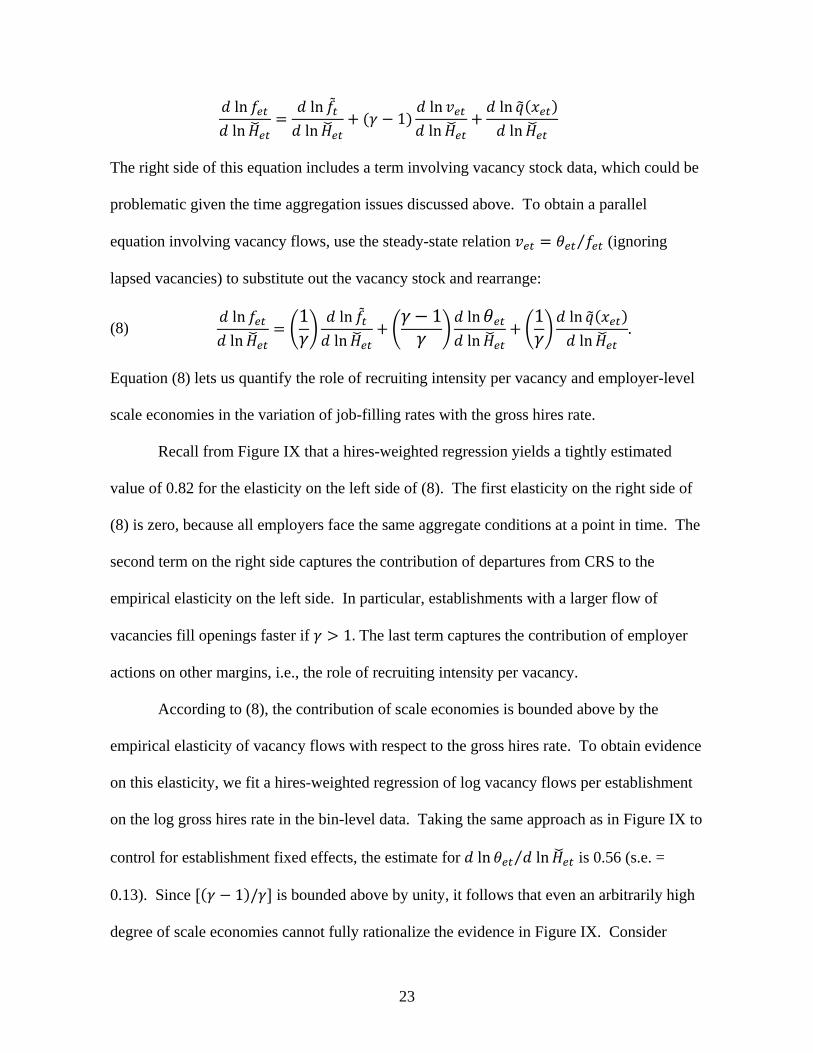
ln

ln

ln

ln1

ln

ln

ln

ln

The right side of this equation includes a term involving vacancy stock data, which could be

problematic given the time aggregation issues discussed above. To obtain a parallel

equation involving vacancy flows, use the steady-state relation ⁄ (ignoring

lapsed vacancies) to substitute out the vacancy stock and rearrange:

(8) ln

ln

1 ln

ln

1 ln

ln

1 ln

ln.

Equation (8) lets us quantify the role of recruiting intensity per vacancy and employer-level

scale economies in the variation of job-filling rates with the gross hires rate.

Recall from Figure IX that a hires-weighted regression yields a tightly estimated

value of 0.82 for the elasticity on the left side of (8). The first elasticity on the right side of

(8) is zero, because all employers face the same aggregate conditions at a point in time. The

second term on the right side captures the contribution of departures from CRS to the

empirical elasticity on the left side. In particular, establishments with a larger flow of

vacancies fill openings faster if 1. The last term captures the contribution of employer

actions on other margins, i.e., the role of recruiting intensity per vacancy.

According to (8), the contribution of scale economies is bounded above by the

empirical elasticity of vacancy flows with respect to the gross hires rate. To obtain evidence

on this elasticity, we fit a hires-weighted regression of log vacancy flows per establishment

on the log gross hires rate in the bin-level data. Taking the same approach as in Figure IX to

control for establishment fixed effects, the estimate for ln ln⁄ is 0.56 (s.e. =

0.13). Since 1 / is bounded above by unity, it follows that even an arbitrarily high

degree of scale economies cannot fully rationalize the evidence in Figure IX. Consider

24

2, an extremely strong scale effect.20 Plugging into (8) with ln ln⁄ 0.56,

scale economies account for only one-third of the fill-rate variation in Figure IX. We

conclude that recruiting intensity per vacancy is the chief force – possibly the only important

force – behind the employer-level relationship of the job-filling rate to the gross hires rate.

Equation (8) also delivers a lower bound on the size of the recruiting intensity

elasticity, ln / ln . In particular, solving (8) for this elasticity and using the

empirical finding that ln ln⁄ ln ln⁄ , it is easy to show that

ln / ln is bounded below by 0.56 for 0 and, moreover, that the implied

elasticity increases with . In short, and regardless of the returns-to-scale parameter , our

evidence in combination with (8) implies that employers substantially increase recruiting

intensity per vacancy as they increase the gross hires rate.

V.C. Returns to Vacancies in the Employer-Level Hiring Technology

The foregoing analysis reveals a major role for recruiting intensity. To sharpen this

point, we consider two sources of evidence on the size of . First, we note that aggregate

matching function studies suggest is close to one. To see why, set q . ≡ and

aggregate in (6) to obtain ln ln ln ln , approximating the sum of log

vacancies by the log of the sum. Thus, scale economies at the micro level carry over to

increasing returns at the aggregate level. As it turns out, few of the many studies

summarized in Petrongolo and Pissarides (2001, Table 3) find evidence of increasing returns

20 From (7), the job-filling rate is proportional to the level of vacancies when γ = 2. From Table I, the ratio of separation rates in the 5000+ category to the 50-249 category is (1.5/3.8)=0.395. Thus, the steady-state vacancy flow at an employer with 5,000 workers is nearly 40 times larger than at one with 50 workers. So γ = 2 implies tremendously faster job filling at the larger employer. While larger and smaller employers may differ in other respects that affect job-filling rates, Tables I and III show no sign of such a powerful scale effect in the pattern of vacancy yields and job-filling rates by employer size.

25

in the aggregate matching function. Yashiv (2000), an exception, obtains results consistent

with = 1.36. Most studies of the aggregate matching function support = 1.

Second, we develop new evidence by fitting a regression derived from (7) to JOLTS

data aggregated to industry employer size cells and pooled over the 2001-2006 period.21

We select the aggregation level and specify the regression model to isolate variation in the

scale of employer hiring activity, as measured by vacancies per establishment. Pooling over

time increases cell density and suppresses cyclical variation in market tightness and

recruiting intensity, both of which would undermine our efforts to isolate scale effects.

Letting i and s index industries and size classes and taking logs in (7) yields

ln ln 1 ln ln ,

where is the job-filling rate in the industry-size cell, ln is a constant that absorbs the

average level of market tightness during the sample period, is the number of vacancies

per establishment in the cell, ln is average recruiting intensity per vacancy, and

captures sampling error in the cell-level data and unobserved differences in matching

efficiency and market tightness.

OLS estimation of this specification gives rise to several econometric concerns.

First, failing to control for recruiting intensity can lead to an omitted variable bias. Second,

OLS estimation suffers from an endogeneity bias if matching efficiency differences partly

drive the variation in . Third, OLS estimation can also lead to a form of division bias. To

see the issue, recall the steady-state approximation / implied by our model of daily

21 We use 12 major industry sectors and 6 size classes. For two industries, the largest size classes have very sparse cells. We therefore aggregate these cells into the next largest size class, providing us with 70 cell-level observations.

26

hiring dynamics. This approximation indicates that measurement errors in v enter into our

model-based estimates of f derived from (3) and (4).

We deal with these concerns as follows. First, we include industry and size class

fixed effects to capture differences in both match efficiency and recruiting intensity across

industries and size classes. Second, we include the average employment growth rate in the

industry-size cell during the sample period, , as a proxy for residual differences in

recruiting intensity per vacancy not captured by the fixed effects. Third, we instrument

ln with the log of employment per establishment in the cell using two stage least squares.

This instrument addresses division bias and we think largely takes care of endogeneity bias.

Differences in the scale of employment across industry-size cells mainly reflect

fundamentals related to product demand, factor costs, and the output production function,

not differences in matching efficiency.

Another potential concern is the regression model’s specification in terms of the

vacancy stock, v, which is subject to time aggregation. To address this concern, we consider

a second regression model specified in terms of vacancy flows, , measured as the average

vacancy flow per establishment in the industry-size cell. Using the steady-state relation,

⁄ , and substituting, our second regression model has the same form as above but

with replacing and a coefficient of 1 / on ln . We estimate both regression

specifications by OLS and two-stage least squares.

Table V presents the results. Three of the four estimates for provide statistically

significant evidence of mild increasing returns to vacancies. In light of our remarks about

potential biases and time aggregation, our preferred estimate uses 2SLS estimation of the

specification with vacancy flows, which yields 1.33. Following the suggestion of a

27

referee, we also estimated specifications without the control. Rather than include an

imperfect control for unobserved variation in recruiting intensity, the idea is to rely on a

bounding argument. In particular, the natural concern is that the recruiting-intensity

component of the error term covaries positively with desired hiring and, hence, with

vacancies. In this case, dropping yields an upwardly biased estimate of . When we re-

estimate without the variable, we obtain results nearly identical to Table V. Thus, our

results in Table V are not sensitive to concerns about the control.

Returning to (8), we can now more precisely quantify the roles of scale economies

and recruiting intensity. Multiplying 1 / 0.33/1.33 by ln ln⁄ 0.56

yields a value less than 0.15 for the second term on the right side of (8), which amounts to a

small fraction of the empirical elasticity on the left side. We conclude, therefore, that the

strong positive relationship between job-filling rates and gross hires rates in Figure IX

overwhelmingly reflects employer decisions to raise recruiting intensity when they increase

the hiring rate. As a corollary, the strong relationship between fill rates and employer growth

rates in Figure VII also reflects the role of recruiting intensity.

We should add that we do not see Table V as the final word on scale economies in

employer-level hiring technologies. Our results say nothing about scale economies in the

creation of job vacancies; they speak only to the effect of vacancy numbers on job-filling

rates. Likewise, they say nothing about scale economies in the use of non-vacancy

recruiting instruments. There is much room for additional investigations into the employer-

level hiring technology using micro data.

28

V.D. Aggregate Implications

We now draw out several aggregate implications of our findings. We work with

CRS at the micro level, so .22 Aggregating (6) yields a generalized matching

function defined over unemployment, vacancies and recruiting intensity per vacancy:

(9) ,

where and .

Here, is the vacancy-weighted mean impact of employer actions on other recruiting

margins. If is time invariant, it folds into the efficiency parameter µ and (9) reduces to

the standard matching function. However, we just established that employers adjust on

other recruiting margins as they vary the gross hires rate, i.e., varies strongly with the

hires rate in the cross section. It stands to reason that , the vacancy-weighted cross-

sectional mean of , varies with the aggregate hires rate.

How important are employer actions on other recruiting margins for the behavior of

aggregate hires? Dividing by employment and taking log differences in (9) yields ∆ ln

∆ ln 1 ∆ ln 1 ∆ ln . Thus to answer the question, we need to know

how varies with over time. As a working hypothesis, we posit that varies with

over time in the same way as varies with in the cross section. That is, we set the

elasticity of with respect to to 0.82. Given a value for α of about one-half, this

working hypothesis yields the tentative conclusion that accounts for about 40% of

22 Although our preferred estimate in Table V is 1.33,we work with the CRS case for several reasons. First, as remarked in Section V.B, the recruiting elasticity implied by (8) rises with . So the CRS case entails a more conservative value (0.82) for the recruiting intensity elasticity. Second, the CRS case simplifies the aggregation in (9) by obviating the need to track the full cross-sectional distribution of vacancies. Third, Table V points to only mild departures from CRS in vacancies. Moreover, most studies of the aggregate matching function support CRS, as we explained at the outset of Section V.C.

29

movements in the aggregate hires rate. Of course, is correlated with and in the time

series, so we cannot attribute 40% of the movements in aggregate hires uniquely to

recruiting intensity. Nevertheless, this calculation suggests that recruiting intensity is an

important proximate determinant of fluctuations in aggregate hires.

Figure X displays the monthly index for recruiting intensity per vacancy implied by

the working hypothesis over the period covered by published JOLTS data. The index

exhibits sizable movements and, most notably, falls by about 20% from early 2007 to late

2009. This large drop in recruiting intensity had a material effect on the evolution of job-

filling rates over this period. To see this point, recall that the job-filling rate is nearly

proportional to the vacancy yield in aggregate data and use (9) to obtain ∆ ln /

∆ ln ⁄ 1 ∆ ln . The vacancy yield rose by 33.5 log points from its average

value in 2007 to its average value in 2009. Given and the recruiting intensity index

in Figure X, we calculate that the vacancy yield would have risen by 42 log points over this

period had recruiting intensity remained at its 2007 level. In other words, the recruiting

intensity drop from 2007 to 2009 substantially repressed the rise in job-filling rates.

Applying the generalized matching function (9) again, we can perform the same type

of calculation for the job-finding rate of unemployed workers. The literature measures this

rate in various ways, so we calculate its log change from 2007 to 2009 in three ways: the

unemployment-to-employment transition rate in gross flows data from the Current

Population Survey (CPS) fell by 49 log points; the unemployment escape rate calculated

using CPS data on unemployment spell durations fell by 64 log points; and the job-finding

rate calculated as H/u fell by 90 log points. The contemporaneous fall in recruiting intensity

per vacancy accounts for about 10% to 20% of the decline in the job-finding rate over this

0.5

30

period, depending on the job-finding rate measure. Given that the recruiting intensity index

remains low through 2011, it continues to contribute to the historically low job-finding rates

for unemployed workers in recent years.

Summarizing: Under our working hypothesis, recruiting intensity accounts for

sizable cyclical movements in aggregate hires, job-filling rates, and job-finding rates. To

develop this conclusion, we built on micro evidence to motivate and construct our index of

recruiting intensity. We recognize, however, that our working hypothesis involves a bit of a

leap because it calibrates a time-series elasticity from cross-sectional evidence. We now

evaluate this working hypothesis and consider several checks of our conclusions about the

importance of recruiting intensity for aggregate fluctuations. Along the way, we develop

additional evidence that the generalized matching function (9) and the recruiting intensity

index in Figure X improve our understanding of aggregate outcomes.

As a first check, if moves as posited with the aggregate rate of hires, the standard

matching function suffers from a particular form of misspecification. Specifically, the

standard function says that the aggregate vacancy yield obeys a simple relationship to

market tightness given by / ⁄ . In contrast, the generalized matching

function (9) yields / ⁄ . Thus, if employers cut back on recruiting

intensity per vacancy in weak labor markets, (9) implies a decline in the vacancy yield

relative to ⁄ . Returning to Figure I, we evaluate this implication for α = 0.5. The

vacancy yield falls well short of the benchmark implied by the standard matching function

after early 2008, and it typically exceeds this benchmark in the stronger labor markets before

2008. This pattern supports the view that employers cut back on average recruiting intensity

per vacancy, , in a weak labor market with a low hires rate.

31

As a second check, we plug aggregate data on hires, vacancies and unemployment

into the standard matching function (5) to back out a “Solow residual” or macro series,

which we then compare to the micro-founded recruiting intensity measure in Figure X.

Figure XI carries out this comparison for α = 0.5 and reveals that the two measures are very

highly correlated over time.23 Note that our micro-based recruiting intensity index varies

much less than one-for-one with the macro-based Solow residual measure. Perhaps random

errors in the data or the matching function (9) attenuate the estimated relationship in Figure

XI, but the macro-based residual series also captures other forms of cyclical misspecification

in the matching function. For example, if search intensity per unemployed worker declines

in weak labor markets along with recruiting intensity per vacancy, then fluctuations in the

macro-based series will exhibit greater amplitude. Davis [2011] reports evidence along

these lines. Thus, we see our analysis of recruiting intensity as providing only a partial

explanation for the matching function breakdown highlighted by Figure I.

Our third check finds the elasticity value that maximizes the fit of a Beveridge curve

relationship augmented by recruiting intensity. Specifically, we regress the log of the

aggregate unemployment rate on the log of the effective vacancy rate , where

ln ln and is the fill rate elasticity with respect to hires. Estimation by nonlinear

least squares yields ̂ = .836 in this approach based entirely on time-series variation, very

close to the value of .820 from the cross-sectional evidence. This result shows that the

recruiting intensity index we constructed using micro evidence performs well in capturing

the aggregate effects of fluctuations in employers’ use of other recruiting instruments.

23 We have verified that the pattern in Figure XI holds for all values of the matching function elasticity α in the range from 0.3 to 0.7. The R-squared values never fall below 0.61 for α in this range, and they exceed 0.9 for ∈ 0.4, 0.7 . The goodness of fit between the two measures is maximized at 0.51. The slope coefficient

in a regression of the micro-based on the macro-based is always less than one-half.

32

Our fourth check considers whether our micro-based generalized matching function

improves the fit of national and regional Beveridge Curves compared to the standard

matching function. Our fit metric is the residual RMSE in a time-series regression of the log

unemployment rate on the log of the observed vacancy rate (standard) or the log effective

vacancy rate (generalized). As reported in Table VI, the generalized matching function

yields a better fitting Beveridge Curve in all cases. The RMSE is 21% smaller for the

specification implied by the standard matching function in the national data and 13-24%

smaller across the four Census regions. We stress that the generalized matching function

considered here does not nest the standard matching function, because it entails a specific

time-series path for recruiting intensity per vacancy.24

V.E. Additional Implications for Theoretical Models

We have now developed several pieces of evidence that point to an important role

for employer actions on other recruiting margins in the hiring process. Obviously, this

evidence presents a challenge to search and matching models that treat vacancies as the sole

or chief instrument that employers manipulate to vary hires. Our evidence and analysis also

present a deeper and less obvious challenge for the standard equilibrium search model:

adding a recruiting intensity margin is not enough, by itself, to reconcile the standard theory

with the evidence. This conclusion follows by considering a version of the standard theory

due to Pissarides [2000, chapter 5] and confronting it with our evidence.

Pissarides analyzes a search equilibrium model with a generalized matching function

similar to (9). In his model, the job-filling rate rises with recruiting intensity, and recruiting

24 In an analogous exercise, online Appendix B reports that the effective labor market tightness ratio more accurately tracks fluctuations in the job-finding rate in national and regional data. See Appendix Table B.3.

33

costs per vacancy are increasing and convex in the employer’s intensity choice.25 Wages are

determined according to a generalized Nash bargain. Given this setup, Pissarides proves that

optimal recruiting intensity is insensitive to aggregate conditions and takes the same value

for all employers (given that all face the same recruiting cost function). As Pissarides

explains, this result follows because employers use the vacancy rate as the instrument for

attracting workers, and they choose recruiting intensity to minimize cost per vacancy.26 The

cost-minimizing intensity choice depends only on properties of the recruiting cost function.

This invariance result implies that the textbook search equilibrium model – extended

to incorporate variable recruiting intensity – cannot account for the evidence in Figures VII

and IV. Those figures show that job-filling rates rise sharply with employer growth rates

and gross hires rates in the cross section. Moreover, the invariance result precludes a role

for recruiting intensity per vacancy in the behavior of aggregate hires. Thus, the standard

theory cannot account for the evidence in Figures X and XI that average recruiting intensity

varies over time and matters for aggregate hires and the job-finding rate. In sum, both the

cross-sectional and time-series evidence are inconsistent with the standard theory.

We do not see this inconsistency as fatal to standard search equilibrium models with

random matching. Rather, we think the evidence calls for a re-evaluation of some of the

building blocks in these models. One candidate for re-evaluation is the standard free entry

condition for new jobs. This condition ensures that vacancies have zero asset value in

equilibrium. In turn, the zero asset value condition plays a key role in leading all employers

to choose the same recruiting intensity. More generally, when job creation costs rise at the

margin and job characteristics differ among employers, the optimal recruiting intensity and

25 His generalized matching function also allows for variable search intensity by unemployed workers, but that aspect of his model is inessential for the discussion at hand. 26 See the discussion related to his equations (5.22) and (5.30).

34

the job-filling rate increase with the opportunity cost of unfilled positions.27 The free entry

condition for new jobs is widely adopted in search and matching models because it

simplifies the analysis of equilibrium. Our evidence indicates that the simplicity and

analytical convenience come at a high cost. Stepping further away from the textbook model

with random matching, there are other mechanisms that potentially generate heterogeneity in

job-filling rates.28 Our evidence is also informative about other theoretical models of hiring

behavior. Figures VII and IX, for example, are hard to square with simple mismatch models.

In these models, an employer fills vacancies quickly if its hiring requirements do not exhaust

the pool of unemployed workers in the local labor market. That is, an employer with modest

hiring needs enjoys a high job-filling rate. In contrast, a rapidly expanding employer is

more likely to exhaust the local pool of available workers. Thus, employers with greater

hiring needs tend to fill vacancies more slowly and experience lower job-filling rates. In

short, the basic mechanism stressed by mismatch models pushes towards a negative cross-

sectional relationship between job-filling rates and employer growth rates.

Directed search models are readily compatible with the evidence in Figures VII and

IX. These models come with a built-in extra recruiting margin, typically in the form of the

employer’s choice of a wage offer posted along with a vacancy announcement. The wage

offer influences the arrival rate of job applicants and the job-filling rate. An employer that

seeks to expand more rapidly both posts more vacancies and offers a more attractive wage.

27 Davis [2001] analyzes an equilibrium search model with these features and shows that it delivers heterogeneity in recruiting intensity per vacancy and job-filling rates. See his equations (14) and (15) and the related discussion. 28 For example, Faberman and Nagypál [2008] show that a model with search on the job, a convex vacancy creation cost, and productivity differences among firms can deliver a positive relationship between the job-filling rate and employer growth rates in the cross section.

35

As a result, the job-filling rate rises with employer growth rates in the cross section. See

Kass and Kircher [2010] for an explicit analysis of this point.

VI. CONCLUDING REMARKS

This study is the first to examine the behavior of vacancies, hires, and vacancy yields

at the establishment level in the Job Openings and Labor Turnover Survey, a large sample of

U.S. employers. We find strong patterns in hiring and vacancy outcomes related to industry,

employer size, the pace of worker turnover, and employer growth rates.

Our study also innovates in several other respects. First, we develop a model of

daily hiring dynamics and a simple moment-matching method that, when applied to JOLTS

data, identifies the flow of new vacancies and the job-filling rate for vacant positions.

Second, we show that job-filling rates rise steeply with the gross hires rate across industries,

employer size classes, worker turnover groups, and employer growth rates – a novel finding

with important implications for theory. Third, we show how to interpret the evidence

through the lens of a generalized matching function and, in particular, how to extract

information about scale economies in the employer-level hiring and how to identify the role

of other recruiting instruments in the hiring process. Fourth, we develop evidence that

employer actions on other recruiting margins account for a large share of movements in

aggregate hires. We also show that our micro-founded generalized matching function fares

better than the standard matching function in accounting for aggregate movements in job-

filling rates and job-finding rates. The effective vacancy concept embedded in our

generalized matching function also leads to a more stable Beveridge curve in national and

regional data. Finally, we show that the standard search equilibrium model cannot explain

the cross-sectional and time-series evidence, even when the model is extended to incorporate

36

a recruiting intensity margin. We also discuss possible modifications to the standard theory

to help account for the evidence.

Much work remains to explain the patterns in vacancy and hiring behavior we

uncover using JOLTS micro data. One partly unresolved issue involves the 42 percent of

hires that occur at establishments with no reported vacancies at the start of the month. Our

model of daily hiring dynamics accounts for two thirds of these hires. The remaining one-

third reflects some combination of model misspecification, systematic underreporting of

vacancies by JOLTS respondents, and hires not mediated through vacancies. As we discuss

in Section 4, evidence from other sources points to an important role for hires not mediated

through vacancies. A fuller analysis of such hires requires information beyond what is

currently available in JOLTS data. We plan to pursue this topic in future work.

37

References

Abraham, Katherine, “Structural/Frictional vs. Deficient Demand Unemployment: Some New Evidence,” American Economic Review, LXXIII (1983), 708-724. Abraham, Katherine, “Help Wanted Advertising, Job Vacancies, and Unemployment,” Brookings Papers on Economic Activity (1987), 207-43. Acemoglu, Daron and Robert Shimer, “Wage and Technology Dispersion,” Review of Economic Studies, LXIV (2000), 585-607. Albrecht, James and Susan Vroman, “A Matching Model with Endogenous Skill Requirements,” International Economic Review, XLIII (2002), 283-305. Andrews, M.J., S. Bradley, D. Stott, and R. Upward, “Successful Employer Search? An Empirical Analysis of Vacancy Duration Using Micro Data,” Economica, LXXV (2008), 455-480. Barron, John M., Mark C. Berger and Dan A. Black, “Employer Search, Training, and Vacancy Duration,” Economic Inquiry, XXXV (1999), 167-192. Berman, Eli, “Help Wanted, Job Needed: Estimates of a Matching Function from Employment Service Data,” Journal of Labor Economics, XV (1997), S251-S292. Blanchard, Oliver J., and Peter Diamond, “The Beveridge Curve,” Brookings Papers on Economic Activity (1989), 1-60. Burdett, Kenneth and Elizabeth Cunningham, “Toward a Theory of Vacancies,” Journal of Labor Economics, XVI (1998), 445–478. Burdett, Kenneth, and Dale T. Mortensen, “Wage Differentials, Employer Size, and Unemployment,” International Economic Review, XXXIX (1998), 257-73. Clark, Kelly A., “The Job Openings and Labor Turnover Survey: What Initial Data Show,” Monthly Labor Review, CXXVII (2004), 12-23. Clark, Kelly A., and Rosemary Hyson , “New Tools for Labor Market Analysis: JOLTS,” Monthly Labor Review, CXXIV (2001), 32-37. Coles, Melvin G., and Eric Smith, “Cross-Section Estimation of the Matching Function: Evidence from England and Wales,” Economica, LXIII (1996), 589-97. Coles, Melvyn and Eric Smith, “Marketplaces and Matching,” International Economic Review, XXXIX (1998), 239-255.

38

Davis, Steven J., “The Quality Distribution of Jobs and the Structure of Wages in Search Equilibrium,” National Bureau of Economic Research Working Paper No. 8434, 2001. Davis, Steven J., Comment on “Job Search, Emotional Well-Being and Job Finding in a Period of Mass Unemployment,” by Robert E. Hall, Brookings Papers on Economic Activity, (2005), 58-78. Davis, Steven J., R. Jason Faberman, and John Haltiwanger, “Recruiting Intensity During and After the Great Recession: National and Industry Evidence,” American Economic Review: Papers & Proceedings, CII (2012), 584-588. Davis, Steven J., R. Jason Faberman, John Haltiwanger, and Ian Rucker, “Adjusted Estimates of Worker Flows and Job Openings in JOLTS,” in Labor in the New Economy, Katharine Abraham, Michael Harper and James Spletzer (eds.), (Chicago, IL: University of Chicago Press, 2010). Davis, Steven J., John C. Haltiwanger, and Scott Schuh, Job Creation and Destruction. (Cambridge, MA: MIT Press, 1996). Dickerson, Andy, “The Distribution and Determinants of Job Vacancies: Evidence from the 2001 Employer Skills Survey,” Institute for Employment Research Working Paper, University of Warwick, Working 2003. Ebrahimy, Eshan and Robert Shimer, “Stock-Flow Matching,” Journal of Economic Theory, CXLV (2010), 1325-1353. Elsby, Michael, Ryan Michaels, and Gary Solon, “The Ins and Out of Cyclical Unemployment,” American Economic Journal: Macroeconomics, I (2009), 84-110. Faberman, R. Jason, “Studying the Labor Market with the Job Openings and Labor Turnover Survey,” in Producer Dynamics: New Evidence from Micro Data, Timothy Dunne, J. Bradford Jensen and Mark J. Roberts (eds.), (Chicago, IL: Chicago Press, 2008). Faberman, R. Jason and Guido Menzio, “Evidence on the Relationship between Recruiting and the Starting Wage,” unpublished, University of Pennsylvania, 2010. Faberman, R. Jason, and Éva Nagypál, “Quits, Worker Recruitment, and Firm Growth: Theory and Evidence,” Federal Reserve Bank of Philadelphia Working Paper No. 08-13, 2008. Fujita, Shigeru and Garey Ramey, “The Cyclicality of Separation and Job Finding Rates,” International Economic Review, L (2009), 415-430. Hall, Robert E., “Job Loss, Job Finding, and Unemployment in the U.S. Economy over the Past Fifty Years,” in 2005 NBER Macroeconomics Annual, Mark Gertler and Kenneth Rogoff (eds.), (Cambridge, MA: National Bureau for Economic Research, 2005a).

39

Hall, Robert E., “Employment Fluctuations with Equilibrium Wage Stickiness,” American Economic Review, XCV (2005b), 50-65. Hansen, Bent, “Excess Demand, Unemployment, Vacancies, and Wages,” Quarterly Journal of Economics, LXXXIV (1970), 1-23. Holzer, Harry J., “Job Vacancy Rates in the Firm: An Empirical Analysis.” Economica LXI (1994), 17-36. Kaas, Leo and Philipp Kircher, “Efficient Firm Dynamics in a Frictional Labor Market,” London School of Economics Working Paper, 2010. Moen, Espen R., “Competitive Search Equilibrium.” Journal of Political Economy, CV (1997), 385-411. Mortensen, Dale T., and Christopher A. Pissarides, “Job Creation and Job Destruction and the Theory of Unemployment.” Review of Economic Studies, LXI (1994), 397-415. Mortensen, Dale T., and Christopher A. Pissarides, “New Developments in Models of Search in the Labor Market,” in Handbook of Labor Economics, Volume 3, Orley Ashenfelter and David Card (eds.), (Amsterdam: Elsevier Science, 1999). Nagypál, Éva, “Labor Market Fluctuations and On-the-Job Search,” Northwestern University Working Paper, 2007. Ours, Jan van and Geert Ridder, “Cyclical Variation in Vacancy Durations and Vacancy Flows.” European Economic Review, XXXV (1991), 1143-1155. Petrongolo, Barbara, and Christopher A. Pissarides, “Looking into the Black Box: A Survey of the Matching Function,” Journal of Economic Literature, XXXIX (2001), 390–431. Petrongolo, Barbara, and Christopher A. Pissarides, “The Ins and Outs of European Unemployment,” American Economic Review, XCVIII (2008), 256-262. Pissarides, Christopher A., “Short-Run Equilibrium Dynamics of Unemployment, Vacancies and Real Wages,” American Economic Review, LXXV (1985), 676-690. Pissarides, Christopher A., Equilibrium Unemployment Theory, second edition (Cambridge, MA: MIT Press, 2000). Rogerson, Richard, Robert Shimer, and Randall Wright, “Search-Theoretic Models of the Labor Market: A Survey,” Journal of Economic Literature, XLIII (2006), 959-88. Shimer, Robert, “The Cyclical Behavior of Equilibrium Unemployment and Vacancies,” American Economic Review XCV (2005), 25-49.

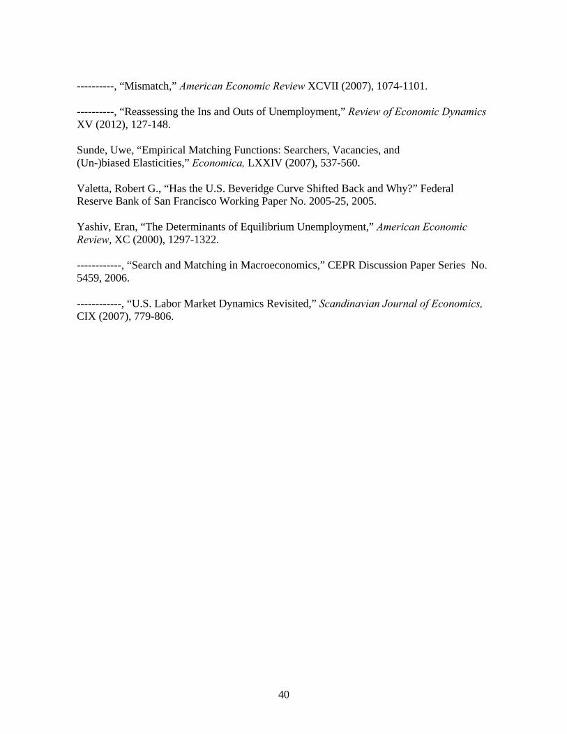
40

----------, “Mismatch,” American Economic Review XCVII (2007), 1074-1101. ----------, “Reassessing the Ins and Outs of Unemployment,” Review of Economic Dynamics XV (2012), 127-148. Sunde, Uwe, “Empirical Matching Functions: Searchers, Vacancies, and (Un-)biased Elasticities,” Economica, LXXIV (2007), 537-560. Valetta, Robert G., “Has the U.S. Beveridge Curve Shifted Back and Why?” Federal Reserve Bank of San Francisco Working Paper No. 2005-25, 2005. Yashiv, Eran, “The Determinants of Equilibrium Unemployment,” American Economic Review, XC (2000), 1297-1322. ------------, “Search and Matching in Macroeconomics,” CEPR Discussion Paper Series No. 5459, 2006. ------------, “U.S. Labor Market Dynamics Revisited,” Scandinavian Journal of Economics, CIX (2007), 779-806.

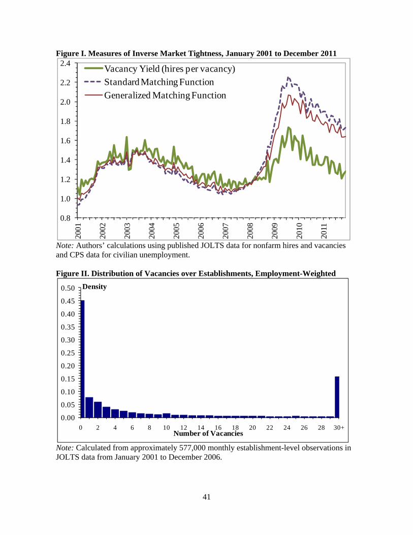
41

Figure I. Measures of Inverse Market Tightness, January 2001 to December 2011

Note: Authors’ calculations using published JOLTS data for nonfarm hires and vacancies and CPS data for civilian unemployment. Figure II. Distribution of Vacancies over Establishments, Employment-Weighted

Note: Calculated from approximately 577,000 monthly establishment-level observations in JOLTS data from January 2001 to December 2006.

0.8

1.0

1.2

1.4

1.6

1.8

2.0

2.2

2.4

2001

2002

2003

2004

2005

2006

2007

2008

2009

2010

2011

Vacancy Yield (hires per vacancy)Standard Matching FunctionGeneralized Matching Function

0.00

0.05

0.10

0.15

0.20

0.25

0.30

0.35

0.40

0.45

0.50

0 2 4 6 8 10 12 14 16 18 20 22 24 26 28 30+Number of Vacancies

Density

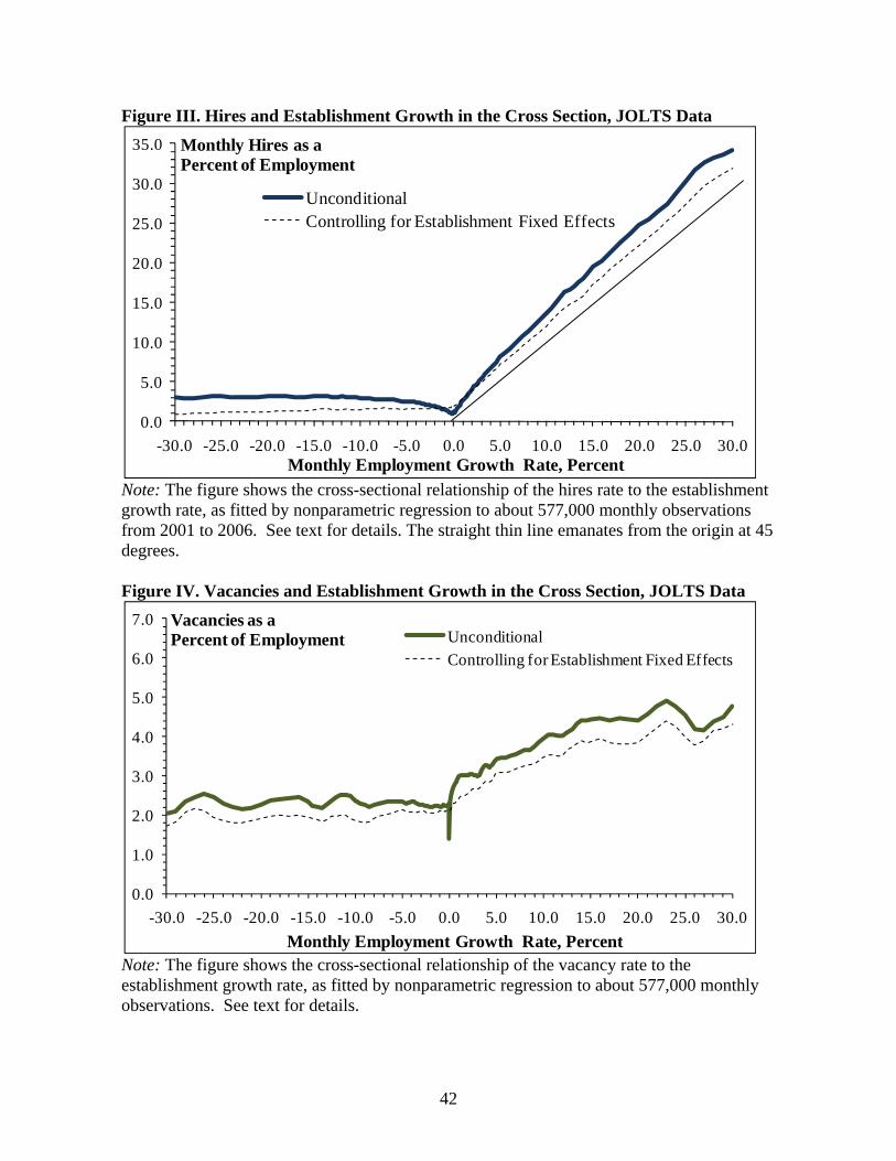
42

Figure III. Hires and Establishment Growth in the Cross Section, JOLTS Data

Note: The figure shows the cross-sectional relationship of the hires rate to the establishment growth rate, as fitted by nonparametric regression to about 577,000 monthly observations from 2001 to 2006. See text for details. The straight thin line emanates from the origin at 45 degrees. Figure IV. Vacancies and Establishment Growth in the Cross Section, JOLTS Data

Note: The figure shows the cross-sectional relationship of the vacancy rate to the establishment growth rate, as fitted by nonparametric regression to about 577,000 monthly observations. See text for details.

0.0

5.0

10.0

15.0

20.0

25.0

30.0

35.0

-30.0 -25.0 -20.0 -15.0 -10.0 -5.0 0.0 5.0 10.0 15.0 20.0 25.0 30.0Monthly Employment Growth Rate, Percent

Monthly Hires as a Percent of Employment

UnconditionalControlling for Establishment Fixed Effects

0.0

1.0

2.0

3.0

4.0

5.0

6.0

7.0

-30.0 -25.0 -20.0 -15.0 -10.0 -5.0 0.0 5.0 10.0 15.0 20.0 25.0 30.0

Monthly Employment Growth Rate, Percent

Vacancies as aPercent of Employment Unconditional

Controlling for Establishment Fixed Effects

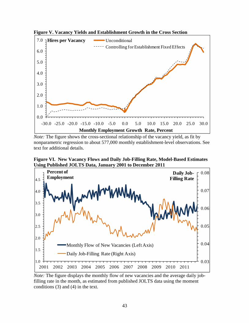
43

Figure V. Vacancy Yields and Establishment Growth in the Cross Section

Note: The figure shows the cross-sectional relationship of the vacancy yield, as fit by nonparametric regression to about 577,000 monthly establishment-level observations. See text for additional details. Figure VI. New Vacancy Flows and Daily Job-Filling Rate, Model-Based Estimates Using Published JOLTS Data, January 2001 to December 2011

Note: The figure displays the monthly flow of new vacancies and the average daily job-filling rate in the month, as estimated from published JOLTS data using the moment conditions (3) and (4) in the text.

0.0

1.0

2.0

3.0

4.0

5.0

6.0

7.0

-30.0 -25.0 -20.0 -15.0 -10.0 -5.0 0.0 5.0 10.0 15.0 20.0 25.0 30.0

Monthly Employment Growth Rate, Percent

Hires per Vacancy Unconditional

Controlling for Establishment Fixed Effects

0.03

0.04

0.05

0.06

0.07

0.08

1.0

1.5

2.0

2.5

3.0

3.5

4.0

4.5

2001 2002 2003 2004 2005 2006 2007 2008 2009 2010 2011

Daily Job-Filling Rate

Percent of Employment

Monthly Flow of New Vacancies (Left Axis)

Daily Job-Filling Rate (Right Axis)

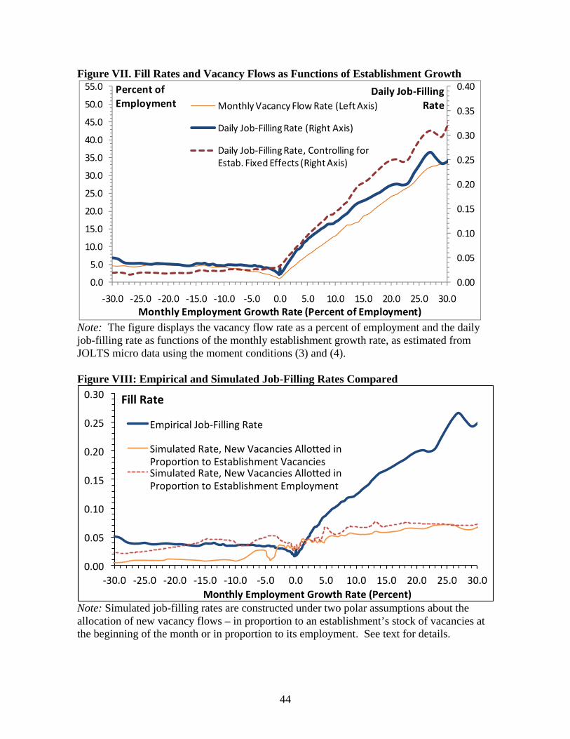
44

Figure VII. Fill Rates and Vacancy Flows as Functions of Establishment Growth

Note: The figure displays the vacancy flow rate as a percent of employment and the daily job-filling rate as functions of the monthly establishment growth rate, as estimated from JOLTS micro data using the moment conditions (3) and (4). Figure VIII: Empirical and Simulated Job-Filling Rates Compared

Note: Simulated job-filling rates are constructed under two polar assumptions about the allocation of new vacancy flows – in proportion to an establishment’s stock of vacancies at the beginning of the month or in proportion to its employment. See text for details.

0.00

0.05

0.10

0.15

0.20

0.25

0.30

0.35

0.40

0.0

5.0

10.0

15.0

20.0

25.0

30.0

35.0

40.0

45.0

50.0

55.0

‐30.0 ‐25.0 ‐20.0 ‐15.0 ‐10.0 ‐5.0 0.0 5.0 10.0 15.0 20.0 25.0 30.0

Daily Job‐Filling 

Rate

Percent of 

Employment

Monthly Employment Growth Rate (Percent of Employment)

Monthly Vacancy Flow Rate (Left Axis)

Daily Job‐Filling Rate (Right Axis)

Daily Job‐Filling Rate, Controlling for Estab. Fixed Effects (Right Axis)

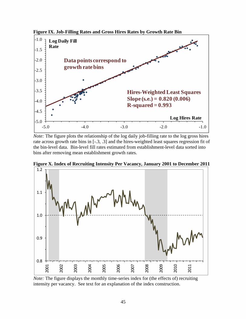
45

Figure IX. Job-Filling Rates and Gross Hires Rates by Growth Rate Bin

Note: The figure plots the relationship of the log daily job-filling rate to the log gross hires rate across growth rate bins in [-.3, .3] and the hires-weighted least squares regression fit of the bin-level data. Bin-level fill rates estimated from establishment-level data sorted into bins after removing mean establishment growth rates. Figure X. Index of Recruiting Intensity Per Vacancy, January 2001 to December 2011

Note: The figure displays the monthly time-series index for (the effects of) recruiting intensity per vacancy. See text for an explanation of the index construction.

-5.0

-4.5

-4.0

-3.5

-3.0

-2.5

-2.0

-1.5

-1.0

-5.0 -4.0 -3.0 -2.0 -1.0

Log Daily Fill Rate

Log Hires Rate

Hires-Weighted Least SquaresSlope (s.e.) = 0.820 (0.006)R-squared = 0.993

Data points correspond to growth rate bins

0.8

0.9

1.0

1.1

1.2

2001

2002

2003

2004

2005

2006

2007

2008

2009

2010

2011

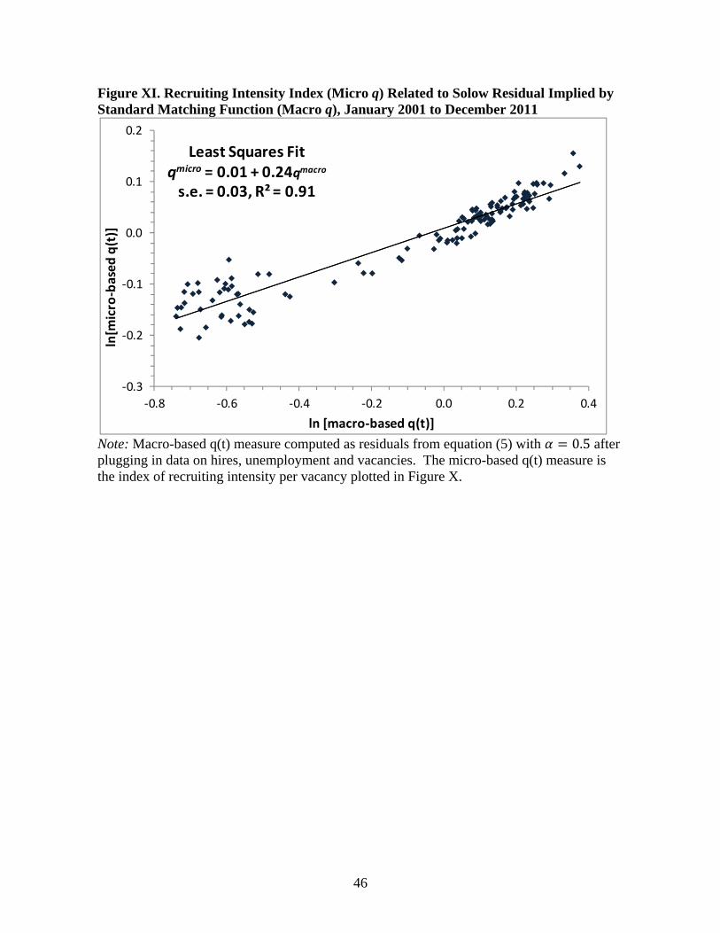
46

Figure XI. Recruiting Intensity Index (Micro q) Related to Solow Residual Implied by Standard Matching Function (Macro q), January 2001 to December 2011

Note: Macro-based q(t) measure computed as residuals from equation (5) with 0.5 after plugging in data on hires, unemployment and vacancies. The micro-based q(t) measure is the index of recruiting intensity per vacancy plotted in Figure X.

Least Squares Fitqmicro = 0.01 + 0.24qmacro

s.e. = 0.03, R² = 0.91

‐0.3

‐0.2

‐0.1

0.0

0.1

0.2

‐0.8 ‐0.6 ‐0.4 ‐0.2 0.0 0.2 0.4

ln[m

icro‐based

 q(t)]

ln [macro‐based q(t)]

47

Table I. Average Monthly Worker Flow Rates, Vacancy Rates and Vacancy Yields by Industry, Size, and Turnover, 2001 to 2006

Hires Rate

SeparationsRate

Vacancy Rate

Vacancy Yield

Employment Share

Nonfarm Employment 3.4 3.2 2.5 1.3 --- Major Industry

Natural Resources & Mining 3.1 3.0 1.5 2.0 0.5 Construction 5.4 5.4 1.7 3.1 5.3 Manufacturing 2.3 2.6 1.7 1.3 11.3 Transport, Wholesale, Utilities 2.7 2.7 1.9 1.4 8.0 Retail Trade 4.5 4.4 2.3 1.9 11.4 Information 2.2 2.4 2.6 0.8 2.4 FIRE 2.3 2.2 2.5 0.9 6.1 Prof. & Business Services 4.6 4.2 3.5 1.3 12.4 Health & Education 2.7 2.3 3.5 0.7 12.7 Leisure & Hospitality 6.3 6.0 3.4 1.8 9.3 Other Services 3.3 3.2 2.3 1.4 4.1 Government 1.6 1.3 1.9 0.8 16.5

Establishment Size Class 0-9 Employees 3.4 3.3 2.0 1.6 12.1 10-49 Employees 4.0 4.0 2.3 1.7 23.2 50-249 Employees 4.0 3.8 2.6 1.5 28.3 250-999 Employees 3.1 2.9 2.8 1.1 17.1 1,000-4,999 Employees 2.1 1.9 3.0 0.7 13.0 5,000+ Employees 1.7 1.5 2.4 0.7 6.4

Worker Turnover Category No Turnover 0 0 1.1 0 24.4 First Quintile 0.5 0.6 1.7 0.3 15.1 Second Quintile 1.3 1.2 2.6 0.5 15.1 Third Quintile 2.4 2.2 2.9 0.8 15.1 Fourth Quintile 4.5 4.3 3.1 1.4 15.1 Fifth Quintile (highest) 13.5 13.0 4.4 3.1 15.1

Notes: Estimates tabulated from our sample of JOLTS micro data, containing 577,268 monthly establishment-level observations from 2001 to 2006. Rates of hires and separations are monthly flows expressed as a percent of employment. The vacancy rate is the stock of open job positions on the last business day of the month expressed as a percent of employment. The vacancy yield is the flow of hires during the month as a ratio to the vacancy stock on the last day of the previous month. The employment share is employment as a percent of total nonfarm employment. Turnover is the sum of the hires rate and the separations rate for the monthly establishment-level observation.

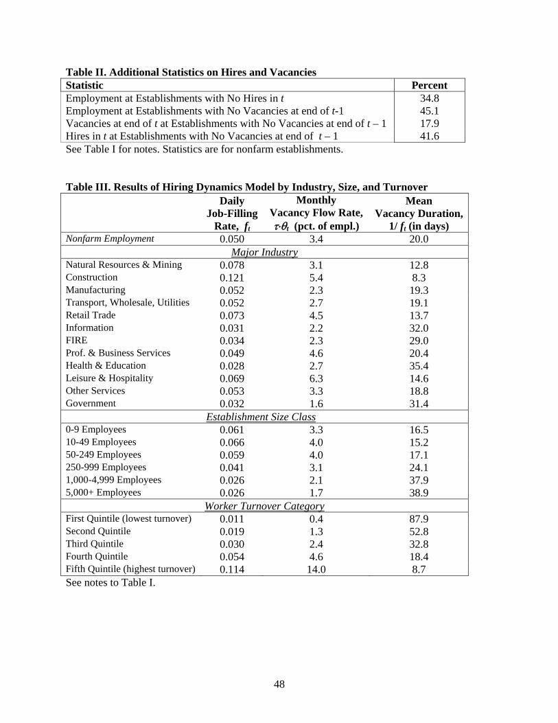
48

Table II. Additional Statistics on Hires and Vacancies Statistic Percent Employment at Establishments with No Hires in t 34.8 Employment at Establishments with No Vacancies at end of t-1 45.1 Vacancies at end of t at Establishments with No Vacancies at end of t – 1 17.9 Hires in t at Establishments with No Vacancies at end of t – 1 41.6 See Table I for notes. Statistics are for nonfarm establishments. Table III. Results of Hiring Dynamics Model by Industry, Size, and Turnover Daily

Job-FillingRate, ft

Monthly Vacancy Flow Rate, t (pct. of empl.)

Mean Vacancy Duration,

1/ ft (in days) Nonfarm Employment 0.050 3.4 20.0

Major Industry Natural Resources & Mining 0.078 3.1 12.8 Construction 0.121 5.4 8.3 Manufacturing 0.052 2.3 19.3 Transport, Wholesale, Utilities 0.052 2.7 19.1 Retail Trade 0.073 4.5 13.7 Information 0.031 2.2 32.0 FIRE 0.034 2.3 29.0 Prof. & Business Services 0.049 4.6 20.4 Health & Education 0.028 2.7 35.4 Leisure & Hospitality 0.069 6.3 14.6 Other Services 0.053 3.3 18.8 Government 0.032 1.6 31.4 Establishment Size Class 0-9 Employees 0.061 3.3 16.5 10-49 Employees 0.066 4.0 15.2 50-249 Employees 0.059 4.0 17.1 250-999 Employees 0.041 3.1 24.1 1,000-4,999 Employees 0.026 2.1 37.9 5,000+ Employees 0.026 1.7 38.9

Worker Turnover Category First Quintile (lowest turnover) 0.011 0.4 87.9 Second Quintile 0.019 1.3 52.8 Third Quintile 0.030 2.4 32.8 Fourth Quintile 0.054 4.6 18.4 Fifth Quintile (highest turnover) 0.114 14.0 8.7 See notes to Table I.

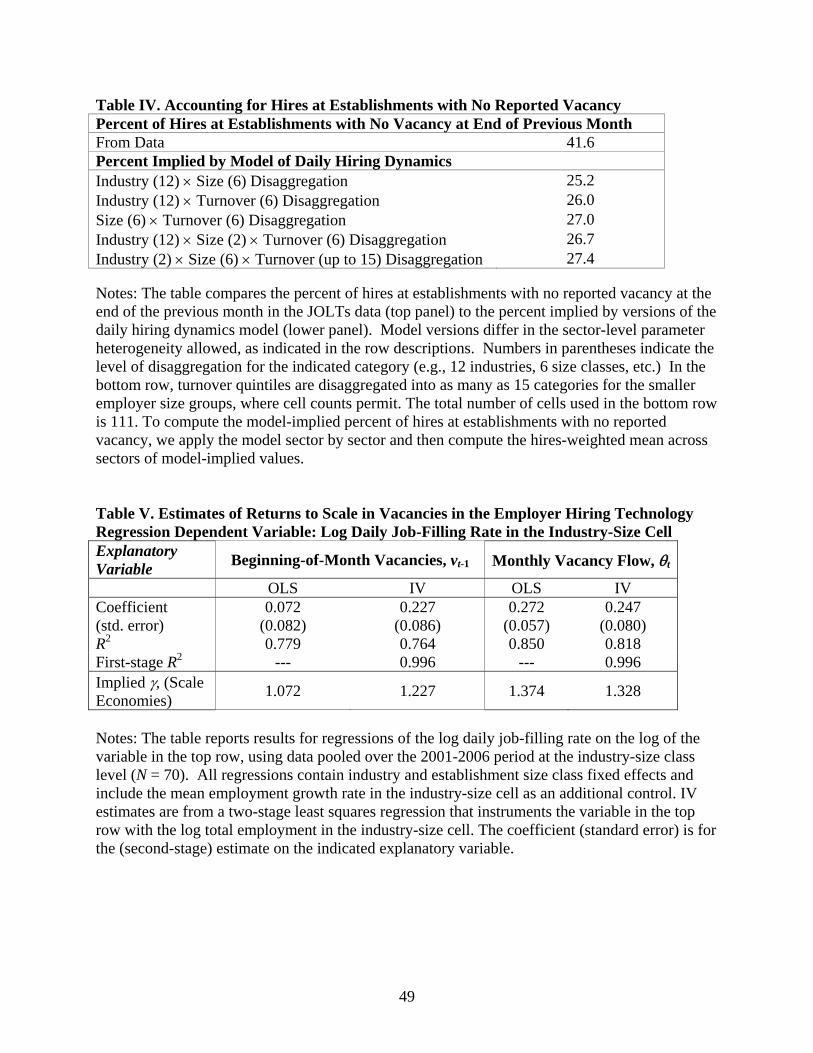
49

Table IV. Accounting for Hires at Establishments with No Reported Vacancy Percent of Hires at Establishments with No Vacancy at End of Previous Month From Data 41.6 Percent Implied by Model of Daily Hiring Dynamics Industry (12) Size (6) Disaggregation 25.2 Industry (12) Turnover (6) Disaggregation 26.0 Size (6) Turnover (6) Disaggregation 27.0 Industry (12) Size (2) Turnover (6) Disaggregation 26.7 Industry (2) Size (6) Turnover (up to 15) Disaggregation 27.4 Notes: The table compares the percent of hires at establishments with no reported vacancy at the end of the previous month in the JOLTs data (top panel) to the percent implied by versions of the daily hiring dynamics model (lower panel). Model versions differ in the sector-level parameter heterogeneity allowed, as indicated in the row descriptions. Numbers in parentheses indicate the level of disaggregation for the indicated category (e.g., 12 industries, 6 size classes, etc.) In the bottom row, turnover quintiles are disaggregated into as many as 15 categories for the smaller employer size groups, where cell counts permit. The total number of cells used in the bottom row is 111. To compute the model-implied percent of hires at establishments with no reported vacancy, we apply the model sector by sector and then compute the hires-weighted mean across sectors of model-implied values. Table V. Estimates of Returns to Scale in Vacancies in the Employer Hiring Technology Regression Dependent Variable: Log Daily Job-Filling Rate in the Industry-Size Cell Explanatory Variable

Beginning-of-Month Vacancies, vt-1 Monthly Vacancy Flow, t

OLS IV OLS IV Coefficient (std. error)

0.072 (0.082)

0.227 (0.086)

0.272 (0.057)

0.247 (0.080)

R2 0.779 0.764 0.850 0.818 First-stage R2 --- 0.996 --- 0.996 Implied , (Scale Economies)

1.072 1.227 1.374 1.328

Notes: The table reports results for regressions of the log daily job-filling rate on the log of the variable in the top row, using data pooled over the 2001-2006 period at the industry-size class level (N = 70). All regressions contain industry and establishment size class fixed effects and include the mean employment growth rate in the industry-size cell as an additional control. IV estimates are from a two-stage least squares regression that instruments the variable in the top row with the log total employment in the industry-size cell. The coefficient (standard error) is for the (second-stage) estimate on the indicated explanatory variable.

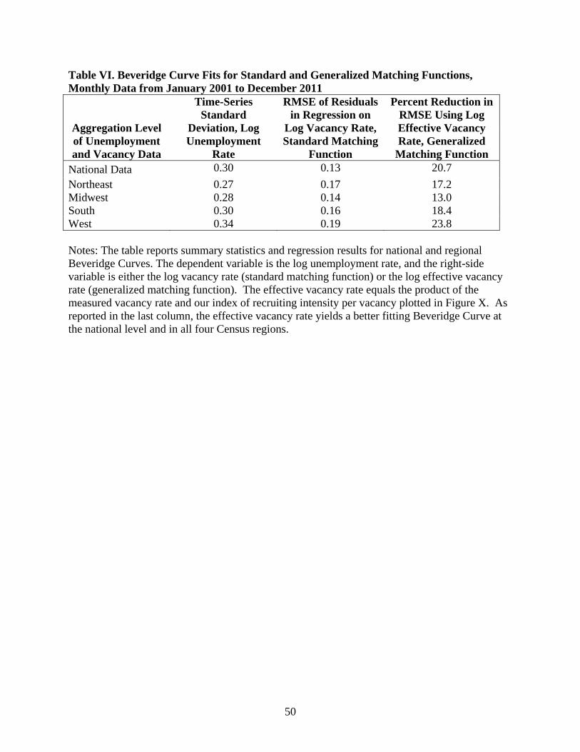
50

Table VI. Beveridge Curve Fits for Standard and Generalized Matching Functions, Monthly Data from January 2001 to December 2011

Aggregation Level of Unemployment and Vacancy Data

Time-Series Standard

Deviation, Log Unemployment

Rate

RMSE of Residuals in Regression on

Log Vacancy Rate, Standard Matching

Function

Percent Reduction in RMSE Using Log Effective Vacancy Rate, Generalized

Matching Function National Data 0.30 0.13 20.7

Northeast 0.27 0.17 17.2 Midwest 0.28 0.14 13.0 South 0.30 0.16 18.4 West 0.34 0.19 23.8 Notes: The table reports summary statistics and regression results for national and regional Beveridge Curves. The dependent variable is the log unemployment rate, and the right-side variable is either the log vacancy rate (standard matching function) or the log effective vacancy rate (generalized matching function). The effective vacancy rate equals the product of the measured vacancy rate and our index of recruiting intensity per vacancy plotted in Figure X. As reported in the last column, the effective vacancy rate yields a better fitting Beveridge Curve at the national level and in all four Census regions.  

1

--Not Intended For Publication--

Appendix Material for “The Establishment-Level Behavior of Vacancies and Hiring”

30 December 2012

Steven J. Davis, University of Chicago and NBER*

R. Jason Faberman, Federal Reserve Bank of Chicago John C. Haltiwanger, University of Maryland and NBER

* Contact information: Steven.Davis@chicagobooth.edu, jfaberman@ frbchi.org, Haltiwan@econ.umd.edu.

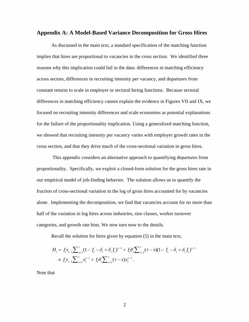
2

Appendix A: A Model-Based Variance Decomposition for Gross Hires

As discussed in the main text, a standard specification of the matching function

implies that hires are proportional to vacancies in the cross section. We identified three

reasons why this implication could fail in the data: differences in matching efficiency

across sectors, differences in recruiting intensity per vacancy, and departures from

constant returns to scale in employer or sectoral hiring functions. Because sectoral

differences in matching efficiency cannot explain the evidence in Figures VII and IX, we

focused on recruiting intensity differences and scale economies as potential explanations

for the failure of the proportionality implication. Using a generalized matching function,

we showed that recruiting intensity per vacancy varies with employer growth rates in the

cross section, and that they drive much of the cross-sectional variation in gross hires.

This appendix considers an alternative approach to quantifying departures from

proportionality. Specifically, we exploit a closed-form solution for the gross hires rate in

our empirical model of job-finding behavior. The solution allows us to quantify the

fraction of cross-sectional variation in the log of gross hires accounted for by vacancies

alone. Implementing the decomposition, we find that vacancies account for no more than

half of the variation in log hires across industries, size classes, worker turnover

categories, and growth rate bins. We now turn now to the details.

Recall the solution for hires given by equation (5) in the main text,

Note that

Ht f

tv

t1(1 f

t

t

tf

t)s1

s1

ft

t( s)(1 f

t

t

tf

t)s1

s1

f

tv

t1x

ts1

s1

ft

t( s)x

ts1

s1

.

3

xts1

s1

1 x

1 x B and

( s)xts1

s1

(1 x) (1 x )

1 x 2 B

1

1 x (1 / )

1 x

where we use the fact that

Therefore, and suppressing time subscripts, we can rewrite the solution for hires as

(A.1)

where , . The term in braces is the sum of old

vacancies and A times the flow of new vacancies, where A converges to unity as

For a given value of and we can calculate A as a function of the daily job-

filling rate, f. Figure A.1 displays this function for and where

.0117 is the mean monthly layoff rate in the JOLTS data. The figure shows that A ranges

from .504 to .872 as f ranges from .01 to .30, and it varies in a narrow range near .6 in the

aggregate time series. Evaluating at sample means for f and yields ̅ 0.5916.

Taking logs in (A.1) yields:

(A.2) log H log(Bf ) log v1 A() .

Using (A.2) with 0.5916, Table A.1 reports the percentage of the cross-sectional

variance in log hires accounted for by vacancies. The table also reports variance

decomposition results based on the “exact” log version of (A.1), which involves no

approximation but is not a true decomposition because of A’s dependence on f. The

ixi

i1

n

x (n 1)xn1 nxn2

(1 x)2.

H Bf v1

1

1 x 1 / 1 x

Bf v1

A

x 1 f f B (1 x ) / (1 x)

.

,

26 (.0117) / 26,

4

rightmost column in Table A.1 uses the steady-state approximation of (2) and (3) in the

main text, which yields log H log log f logv.

If hires are proportional to vacancies in the cross section, then all explanatory

power in the variance decompositions loads onto the vacancy term. Contrary to this

implication, vacancies account for half or less of the cross-sectional variance in log hires.

This conclusion holds for all three variants of the cross-sectional variance decomposition

for log hires. Thus, the variance decomposition results in Table A.1 confirm the

conclusion we drew in the main text that there are large departures from a proportional

relationship between vacancies and hires in the cross section. Moreover, the failure of

the proportionality implication across growth rate bins rules out an explanation that rests

on sectoral differences in matching efficiency. That leaves recruiting intensity and scale

economies as potential explanations for the failure of the proportionality implication.

The variance decomposition results developed in this appendix cannot

discriminate between these two explanations. In that respect, the variance decomposition

is less informative than the generalized matching function analysis in the main text.

Nevertheless, we think the variance decomposition approach is a useful check, because it

imposes fewer assumptions. It is reassuring that the variance decomposition results are

consistent with the matching function analysis in the main text.

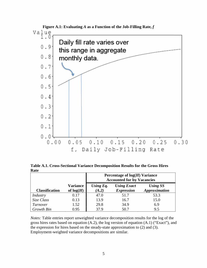
TablRate

CInduSizeTurnGro

Notesgrossthe exEmpl

Figure A

e A.1. Cross

Classificationustry e Class nover wth Bin

s: Table entrs hires rates bxpression foloyment-wei

.1: Evaluati

s-Sectional

n

Variaof log

0.10.11.50.9

ries report unbased on equr hires basedighted varian

ing A as a F

Variance D

ance g(H)

Usi(A

7 43 12 25 3

nweighted vuation (A.2)d on the steance decompo

5

Function of t

Decompositio

PercenAccou

ing Eq. (A.2)

UE

47.0 13.9 29.8 37.9

ariance deco, the log ver

ady-state appositions are s

the Job-Fill

on Results f

ntage of log(unted for by

Using ExactExpression

51.7 16.7 34.9 50.7

omposition rrsion of equaproximation similar.

ling Rate, f

for the Gros

(H) Variancy Vacancies

t UsinApprox

5169

results for thation (A.1) (“to (2) and (3

ss Hires

ce s

ng SS ximation 3.3 5.0

6.9 9.5

he log of the “Exact”), an3).

nd

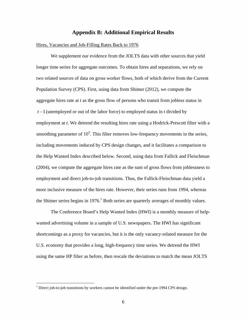
6

Appendix B: Additional Empirical Results

Hires, Vacancies and Job-Filling Rates Back to 1976

We supplement our evidence from the JOLTS data with other sources that yield

longer time series for aggregate outcomes. To obtain hires and separations, we rely on

two related sources of data on gross worker flows, both of which derive from the Current

Population Survey (CPS). First, using data from Shimer (2012), we compute the

aggregate hires rate at t as the gross flow of persons who transit from jobless status in

(unemployed or out of the labor force) to employed status in t divided by

employment at t. We detrend the resulting hires rate using a Hodrick-Prescott filter with a

smoothing parameter of 105. This filter removes low-frequency movements in the series,

including movements induced by CPS design changes, and it facilitates a comparison to

the Help Wanted Index described below. Second, using data from Fallick and Fleischman

(2004), we compute the aggregate hires rate as the sum of gross flows from joblessness to

employment and direct job-to-job transitions. Thus, the Fallick-Fleischman data yield a

more inclusive measure of the hires rate. However, their series runs from 1994, whereas

the Shimer series begins in 1976.1 Both series are quarterly averages of monthly values.

The Conference Board’s Help Wanted Index (HWI) is a monthly measure of help-

wanted advertising volume in a sample of U.S. newspapers. The HWI has significant

shortcomings as a proxy for vacancies, but it is the only vacancy-related measure for the

U.S. economy that provides a long, high-frequency time series. We detrend the HWI

using the same HP filter as before, then rescale the deviations to match the mean JOLTS

1 Direct job-to-job transitions by workers cannot be identified under the pre-1994 CPS design.

1t

7

vacancy rate in the overlapping period.2 We use the detrended rescaled HWI in the first

month of each quarter as a proxy for vacancies and match it to the monthly average CPS-

based hires rates in the same quarter when computing the HWI-CPS vacancy yield.

Figures B.1 and B.2 draw on JOLTS, CPS, and HWI sources to plot aggregate

hires, vacancies and vacancy yields. Figure B.1 shows the aggregate hiring and vacancy

rates, expressed as percentages of employment. The HWI and the JOLTS-based measures

show strong pro-cyclical patterns for hires and vacancies.3 In contrast, the CPS-based

measures show little cyclicality in the hires rate. HP filtering in the Shimer measure

removes a secular decline in hiring observed in other research (e.g., Faberman, 2008 and

Davis et al., 2006). The correlation between the log vacancy yield and log tightness is

-0.85 in the detrended CPS and HWI data from 1975Q2 to 2007Q2 and -0.88 in the

JOLTS data from 2001Q1 to 2011Q4.

We also estimate the job-filling rate using CPS data on new hires and the

detrended Help Wanted Index. These data are less suitable for our methods, but they

provide longer time series for drawing inference about cyclical patterns. Figure B.3

reports the results and shows pronounced counter-cyclical variation in the job-filling rate,

with sharp increases during recessions. All three sources show increasing fill rates during

the recession of 2001, but the increase is less abrupt in the JOLTS data, and it extends for

an additional two years beyond the NBER-dated recession end. (Aggregate employment

continued to contract through the middle of 2003.) In short, the available evidence

2 This approach to the HWI follows Abraham (1987) and Shimer (2012), who discuss the measurement issues in detail. See also Kroft and Pope (2008). 3 The economy was in recession from March to November 2001 according to NBER dating, but employment continued to contract until the middle of 2003.

8

clearly points to strongly counter-cyclical movements in job-filling rates – in line with

the view that employers find it easier to recruit suitable workers in weak labor markets.

Nevertheless, the JOLTS and CPS-HWI series for the job-filling rate are rather

imperfectly correlated during the period of overlap. These discrepancies between JOLTS

and CPS-HWI measures are noteworthy, because quantitative analyses of search and

matching models have relied heavily on CPS-HWI data. One potential explanation is

cyclical variation in the recruiting channels used by employers to hire workers. Recall

that the HWI reflects help-wanted advertising volume in a sample of U.S. newspapers. In

contrast, the JOLTS program elicits information about a broader concept of vacancies

and is not confined to a single recruiting method. Russo, Gorter and Schettkat (2001)

report that Dutch employers alter the mix of recruitment methods as labor market

tightness varies and, in particular, that they rely less heavily on paid advertisements in

weak labor markets.

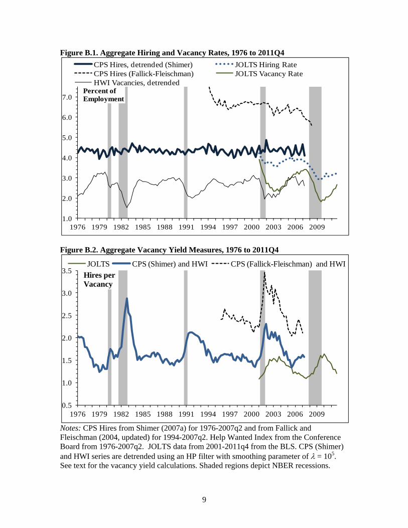
9

Figure B.1. Aggregate Hiring and Vacancy Rates, 1976 to 2011Q4

Figure B.2. Aggregate Vacancy Yield Measures, 1976 to 2011Q4

Notes: CPS Hires from Shimer (2007a) for 1976-2007q2 and from Fallick and Fleischman (2004, updated) for 1994-2007q2. Help Wanted Index from the Conference Board from 1976-2007q2. JOLTS data from 2001-2011q4 from the BLS. CPS (Shimer) and HWI series are detrended using an HP filter with smoothing parameter of = 105. See text for the vacancy yield calculations. Shaded regions depict NBER recessions.

1.0

2.0

3.0

4.0

5.0

6.0

7.0

1976 1979 1982 1985 1988 1991 1994 1997 2000 2003 2006 2009

Percent of Employment

CPS Hires, detrended (Shimer) JOLTS Hiring RateCPS Hires (Fallick-Fleischman) JOLTS Vacancy RateHWI Vacancies, detrended

0.5

1.0

1.5

2.0

2.5

3.0

3.5

1976 1979 1982 1985 1988 1991 1994 1997 2000 2003 2006 2009

Hires perVacancy

JOLTS CPS (Shimer) and HWI CPS (Fallick-Fleischman) and HWI

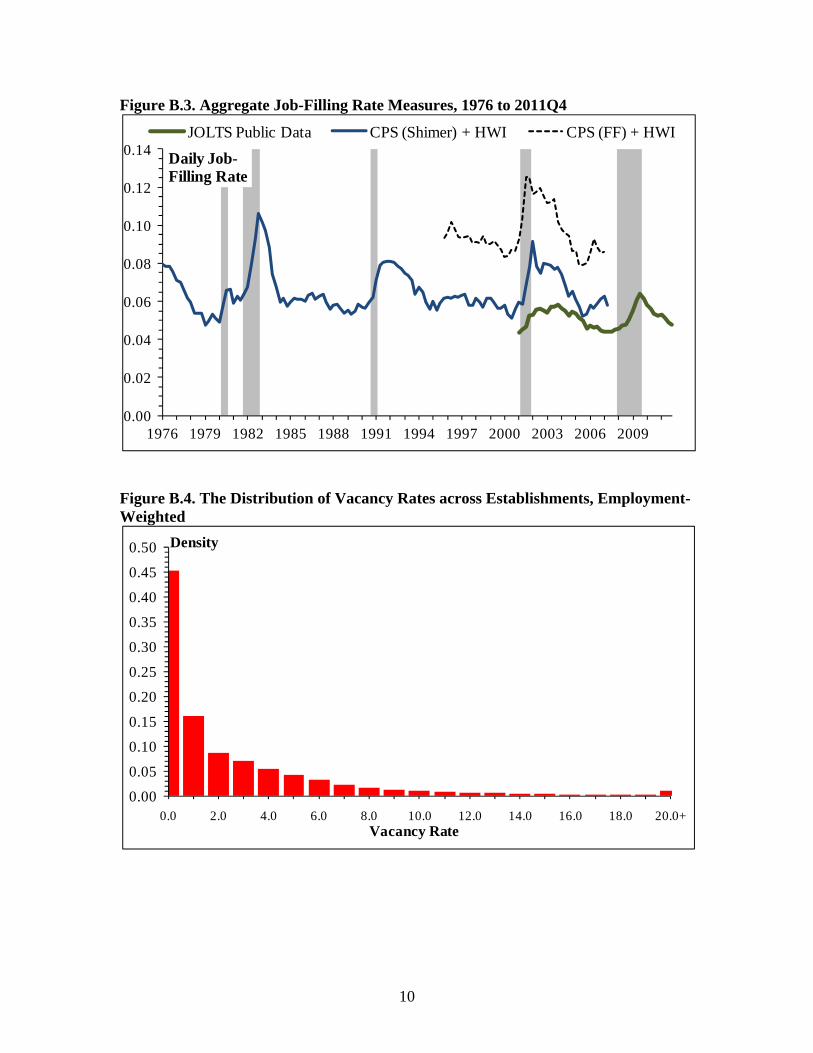
10

Figure B.3. Aggregate Job-Filling Rate Measures, 1976 to 2011Q4

Figure B.4. The Distribution of Vacancy Rates across Establishments, Employment-Weighted

0.00

0.02

0.04

0.06

0.08

0.10

0.12

0.14

1976 1979 1982 1985 1988 1991 1994 1997 2000 2003 2006 2009

Daily Job-Filling Rate

JOLTS Public Data CPS (Shimer) + HWI CPS (FF) + HWI

0.00

0.05

0.10

0.15

0.20

0.25

0.30

0.35

0.40

0.45

0.50

0.0 2.0 4.0 6.0 8.0 10.0 12.0 14.0 16.0 18.0 20.0+Vacancy Rate

Density

11

Additional Cross-Sectional Statistics and Results

Figure B.4 plots the employment-weighted distribution of vacancy rates in the

establishment-level JOLTS data. See Figure II in the main text for the corresponding

distribution of vacancy numbers.

As reported in Table B.1, there is much variation in the frequency of hires and

vacancies across industries, employer size classes, and worker turnover groups.

Industries with the highest worker turnover rates (Table I) have the highest employment-

weighted incidence of establishments with no reported vacancies. The same pattern holds

across worker turnover quintiles, setting aside establishments with no worker turnover.

In addition, nearly half of all hires by employers in the top worker turnover quintile occur

at establishments with no reported vacancies going into the month. Recall from Table I

that worker turnover is 26.5% of employment per month for establishments in this group.

Given these results, it must be the case that vacancy durations are extremely short for

these employers, or that a large fraction of their hires are not mediated through vacancies.

Figure B.5 displays the relationship between the fill rate and the gross hires rate

across industries, size classes and worker turnover categories. The fitted relationship is

very similar to the one across growth rate bins in Figure IX. In short, the job-filling rate

displays a strong positive relationship to the gross hires rate across industries, size

classes, worker turnover groups and employer growth rate bins. This is a novel finding

and, as we show in the main text, it has important implications for theoretical models.

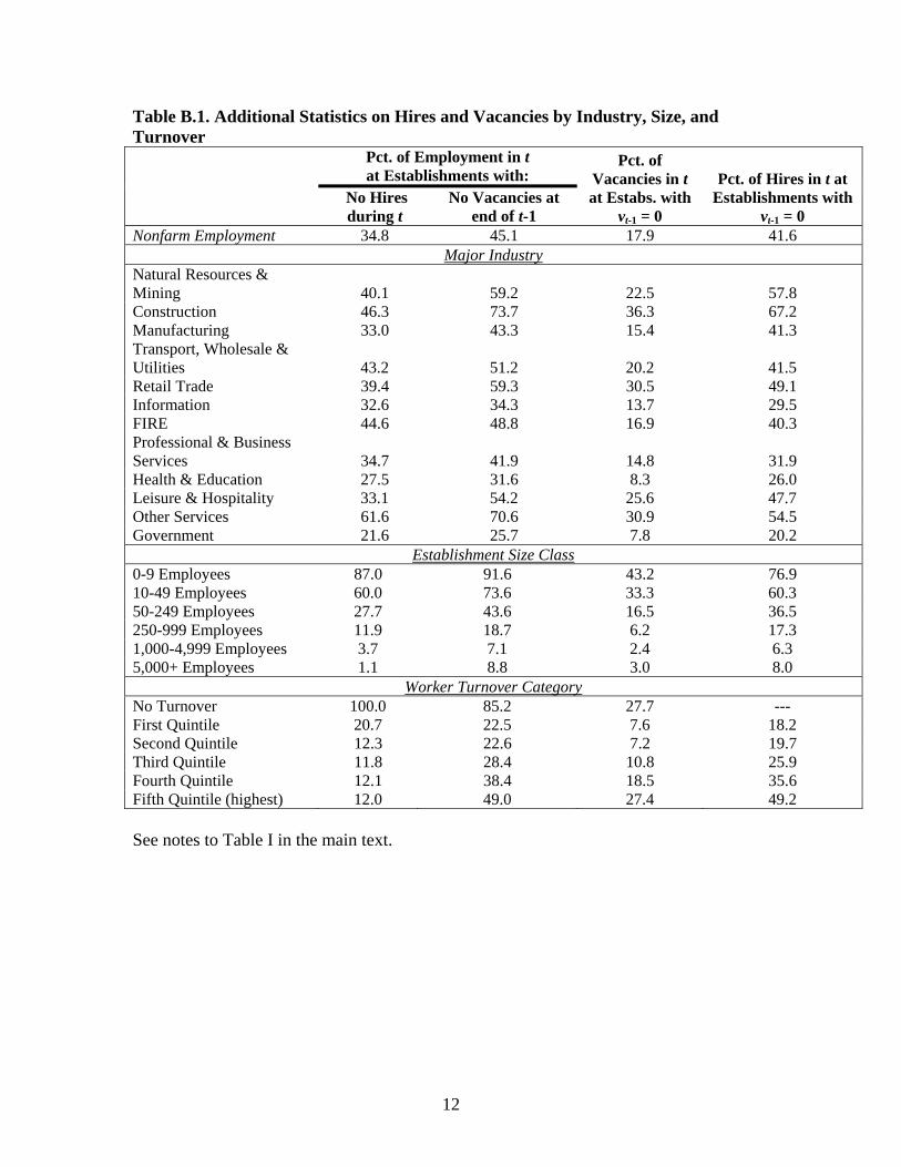
12

Table B.1. Additional Statistics on Hires and Vacancies by Industry, Size, and Turnover Pct. of Employment in t

at Establishments with: Pct. of

Vacancies in t at Estabs. with

vt-1 = 0

Pct. of Hires in t at Establishments with

vt-1 = 0 No Hires during t

No Vacancies at end of t-1

Nonfarm Employment 34.8 45.1 17.9 41.6 Major Industry

Natural Resources & Mining 40.1 59.2 22.5 57.8 Construction 46.3 73.7 36.3 67.2 Manufacturing 33.0 43.3 15.4 41.3 Transport, Wholesale & Utilities 43.2 51.2 20.2 41.5 Retail Trade 39.4 59.3 30.5 49.1 Information 32.6 34.3 13.7 29.5 FIRE 44.6 48.8 16.9 40.3 Professional & Business Services 34.7 41.9 14.8 31.9 Health & Education 27.5 31.6 8.3 26.0 Leisure & Hospitality 33.1 54.2 25.6 47.7 Other Services 61.6 70.6 30.9 54.5 Government 21.6 25.7 7.8 20.2

Establishment Size Class 0-9 Employees 87.0 91.6 43.2 76.9 10-49 Employees 60.0 73.6 33.3 60.3 50-249 Employees 27.7 43.6 16.5 36.5 250-999 Employees 11.9 18.7 6.2 17.3 1,000-4,999 Employees 3.7 7.1 2.4 6.3 5,000+ Employees 1.1 8.8 3.0 8.0

Worker Turnover Category No Turnover 100.0 85.2 27.7 --- First Quintile 20.7 22.5 7.6 18.2 Second Quintile 12.3 22.6 7.2 19.7 Third Quintile 11.8 28.4 10.8 25.9 Fourth Quintile 12.1 38.4 18.5 35.6 Fifth Quintile (highest) 12.0 49.0 27.4 49.2 See notes to Table I in the main text.

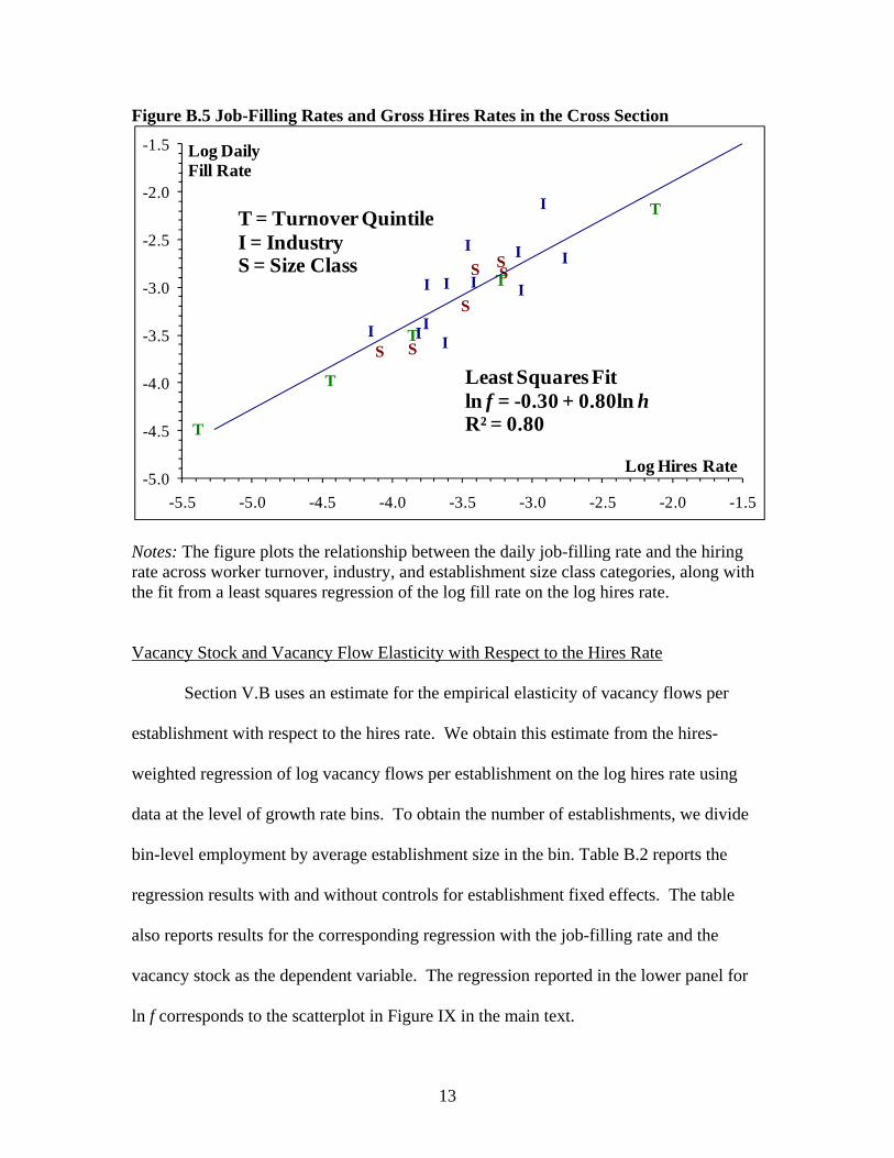
13

Figure B.5 Job-Filling Rates and Gross Hires Rates in the Cross Section

Notes: The figure plots the relationship between the daily job-filling rate and the hiring rate across worker turnover, industry, and establishment size class categories, along with the fit from a least squares regression of the log fill rate on the log hires rate.

Vacancy Stock and Vacancy Flow Elasticity with Respect to the Hires Rate

Section V.B uses an estimate for the empirical elasticity of vacancy flows per

establishment with respect to the hires rate. We obtain this estimate from the hires-

weighted regression of log vacancy flows per establishment on the log hires rate using

data at the level of growth rate bins. To obtain the number of establishments, we divide

bin-level employment by average establishment size in the bin. Table B.2 reports the

regression results with and without controls for establishment fixed effects. The table

also reports results for the corresponding regression with the job-filling rate and the

vacancy stock as the dependent variable. The regression reported in the lower panel for

ln f corresponds to the scatterplot in Figure IX in the main text.

I

I

I I

I

II

I

I

I

I

I

S SS

S

SS

T

T

T

T

T

Least Squares Fitln f = -0.30 + 0.80ln hR² = 0.80

-5.0

-4.5

-4.0

-3.5

-3.0

-2.5

-2.0

-1.5

-5.5 -5.0 -4.5 -4.0 -3.5 -3.0 -2.5 -2.0 -1.5

Log Daily Fill Rate

Log Hires Rate

T = Turnover QuintileI = IndustryS = Size Class

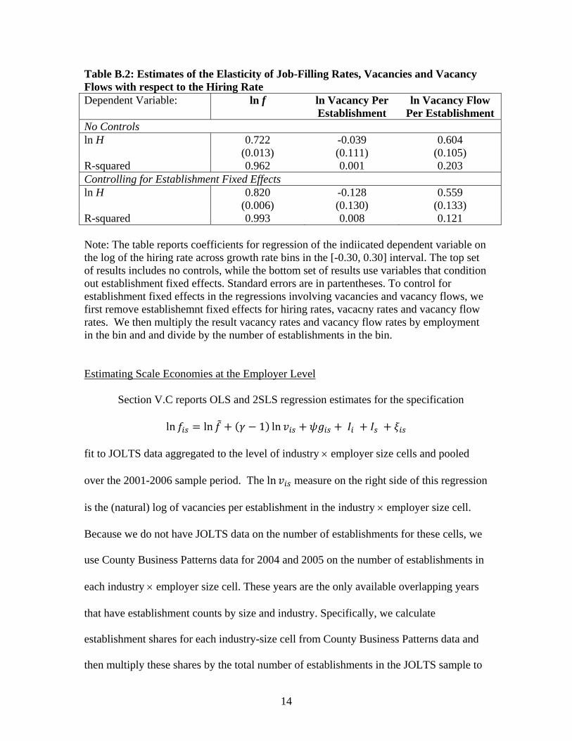
14

Table B.2: Estimates of the Elasticity of Job-Filling Rates, Vacancies and Vacancy Flows with respect to the Hiring Rate Dependent Variable: ln f ln Vacancy Per

Establishment ln Vacancy Flow

Per Establishment No Controls ln H 0.722

(0.013) -0.039 (0.111)

0.604 (0.105)

R-squared 0.962 0.001 0.203 Controlling for Establishment Fixed Effects ln H 0.820

(0.006) -0.128 (0.130)

0.559 (0.133)

R-squared 0.993 0.008 0.121 Note: The table reports coefficients for regression of the indiicated dependent variable on the log of the hiring rate across growth rate bins in the [-0.30, 0.30] interval. The top set of results includes no controls, while the bottom set of results use variables that condition out establishment fixed effects. Standard errors are in partentheses. To control for establishment fixed effects in the regressions involving vacancies and vacancy flows, we first remove establishemnt fixed effects for hiring rates, vacacny rates and vacancy flow rates. We then multiply the result vacancy rates and vacancy flow rates by employment in the bin and and divide by the number of establishments in the bin.

Estimating Scale Economies at the Employer Level

Section V.C reports OLS and 2SLS regression estimates for the specification

ln ln 1 ln

fit to JOLTS data aggregated to the level of industry employer size cells and pooled

over the 2001-2006 sample period. The ln measure on the right side of this regression

is the (natural) log of vacancies per establishment in the industry employer size cell.

Because we do not have JOLTS data on the number of establishments for these cells, we

use County Business Patterns data for 2004 and 2005 on the number of establishments in

each industry employer size cell. These years are the only available overlapping years

that have establishment counts by size and industry. Specifically, we calculate

establishment shares for each industry-size cell from County Business Patterns data and

then multiply these shares by the total number of establishments in the JOLTS sample to

15

get our figure for the number of establishments in each cell. We calculate the average

vacancy stock per establishment in the cell as total vacancies in the cell divided by

number of establishments in the cell. We take the same approach to calculate the average

vacancy flow per establishment in the cell.

Tracking the Job-Finding Rate Using Standard and Generalized Matching Functions

Table VI in the main text compares Beveridge Curve fits using observed

vacancies to our measure of effective vacancies. We repeat the same type of exercise

here using the job-finding rate as the dependent variable and the market tightness ratio as

the explanatory variable. Specifically, we regress the log of the job-finding rate

measured as JOLTS hires per unemployed worker on the log of one of two measures of

labor market tightness: the (v/u) ratio implied by the standard matching function, or the

ratio of effective vacancies to unemployment / implied by the generalized matching

function. Here , where is the recruiting intensity index in Figure X. Our goal

is to assess which tightness measure performs better in tracking the job-finding rate.

Table B.3 reports the results and shows that the effective market tightness

measure corresponding to the generalized matching function outperforms the standard

market tightness measure at the national level and in all four Census regions. The residual

RMSE is 17.7 percent lower at the national level using the effective market tightness

measure and 15.3 to 28.0 percent lower across the four Census regions.

16

Table B.3 Trackng the Job-Finding Rate Using Market Tightness Measures Implied by the Standard and Generalized Matching Functions, Monthly Data from January 2001 to December 2011 Dependent variable: job-finding rate measured as H/u,

Aggregation Level

Time-Series Standard Deviation of Log Job-Finding

Rate

Residual RMSE in Regression on (v/u), Standard Matching

Function

Percent Reduction in RMSE

Using (v’/u), Generalized

Matching Function National Data 0.40 0.08 17.7

Northeast 0.34 0.12 28.0 Midwest 0.37 0.08 21.3 South 0.42 0.11 15.3 West 0.47 0.12 17.3 Notes: The regressions reported in Table B.3 parallel the ones reported in Table VI except for the use of the job-finding rate as the dependent variable and the market tightness ratio as the explanatory variable.

Additional References for the Online Appendix Fallick, Bruce and Charles A. Fleischman, “Employer-to-Employer Flows in the U.S. Labor Market: The Complete Picture of Gross Worker Flows,” Federal Reserve Board of Governors, Finance and Economics Discussion Series No. 2004-34, 2004. Kroft, Kory and Devin G. Pope, “Does Online Search Crowd Out Traditional Search and Improve Matching Efficiency? Evidence from Craigslist,” Working Paper, Wharton School, 2008. Russo, Giovanni, Cees Gorter and Ronald Schettkat, “Searching, Hiring and Labour Market Conditions,” Labour Economics, VIII (2001), 553-571.