Embed Size (px)
Citation preview
The Exchange of Energy, Water and Carbon Dioxide
between Wet Arctic Tundra and the Atmosphere
at the Lena River Delta, Northern Siberia
Dissertation
zur Erlangung des Doktorgrades der Naturwissenschaften
im Fachbereich Geowissenschaften der Universität Hamburg
vorgelegt von
Lars Kutzbach
aus Husum
Hamburg 2006
Als Dissertation angenommen vom Fachbereich Geowissenschaften
der Universität Hamburg
auf Grund der Gutachten von Prof. Dr. Eva-Maria Pfeiffer
und Prof. Dr. Hans-Wolfgang Hubberten
Hamburg, den 31.01.2006
Prof. Dr. Kay-Christian Emeis
Dekan
des Fachbereichs Geowissenschaften
Diese Dissertation ist neben der digitalen Form auch in Druckform veröffentlicht: Kutzbach, Lars (2006): Berichte zur Polar- und Meeresforschung, 541. Alfred-Wegener-Institut für Polar- und Meeresforschung, Am Handelshafen 12, D-27570 Bremerhaven, Deutschland. ISSN 1618-3193, 157 S..
Contents
Contents
I SUMMARY ..................................................................................................................... III
II ZUSAMMENFASSUNG ..................................................................................................V
III ACKNOWLEDGEMENTS ..........................................................................................VII
IV LIST OF TABLES .......................................................................................................... IX
V LIST OF FIGURES ........................................................................................................ IX
VI LIST OF SYMBOLS AND ABBREVIATIONS .........................................................XII
1 INTRODUCTION AND OBJECTIVES ........................................................ 1
2 INVESTIGATION AREA ............................................................................... 6
2.1 The Lena River Delta............................................................................................6
2.2 Samoylov Island.....................................................................................................7
2.3 The Climate..........................................................................................................11
3 METHODS...................................................................................................... 13
3.1 Eddy Covariance Measurements .......................................................................13 3.3.1 General Set-up ................................................................................................13 3.3.2 The Sonic Anemometer ..................................................................................17 3.3.3 The Infrared Gas Analyser for CO2 and H2O (IRGA)....................................18 3.3.4 Processing of Eddy Covariance Fluxes...........................................................20
3.2 Supporting Meteorological Measurements.......................................................23
3.3 Soil-Meteorological Measurements ...................................................................26
3.4 Model Approaches...............................................................................................30 3.4.1 Evaluation of the Energy Balance...................................................................30 3.4.2 Modelling of Latent and Sensible Heat Fluxes...............................................32 3.4.3 Modelling of the CO2 Budget .........................................................................35
4 RESULTS........................................................................................................ 38
4.1 Meteorological Conditions..................................................................................38 4.1.1 Overview of the Years 2003 and 2004 ...........................................................38 4.1.2 The Campaign 2003........................................................................................39 4.1.3 The Campaign 2004........................................................................................42
I
Contents
4.2 Wind and Turbulence Characteristics ..............................................................44
4.3 Energy Fluxes ......................................................................................................49 4.3.1 Time Series of the Energy Fluxes 2003 and 2004 ..........................................49 4.3.2 Influence of Advection on the Energy Partitioning ........................................52 4.3.3 The Diurnal Cycle of the Energy Fluxes ........................................................54 4.3.4 Seasonal Progression of the Energy Partitioning............................................57 4.3.5 Estimated Annual Energy Budget...................................................................58 4.3.6 Energy Balance Closure..................................................................................63
4.4 Water Budget.......................................................................................................64
4.5 Carbon Dioxide Fluxes........................................................................................69 4.5.1 Time Series of CO2 Fluxes 2003 and 2004.....................................................69 4.5.2 The Diurnal Cycle of CO2 Fluxes...................................................................73 4.5.3 The Regulation of CO2 Fluxes........................................................................75 4.5.4 Seasonal CO2 Balance ....................................................................................80 4.5.5 Estimated Annual CO2 Budget .......................................................................82
5 DISCUSSION.................................................................................................. 84
5.1 The Energy and Water Balance at Wet Arctic Tundra...................................84
5.2 The Carbon Dioxide Balance of Wet Arctic Tundra .......................................97 5.2.1 The Tundra Carbon Pool under Climate Change............................................97 5.2.2 Gross Photosynthesis Pgross .............................................................................97 5.2.3 Ecosystem Respiration Reco...........................................................................102 5.2.4 Net ecosystem Exchange NEE......................................................................105
5.3 The Coupling of the CO2 Budget with the Energy and Water Balance cccc- Response to Climatic Change ........................................................................107
5.4 Perspectives........................................................................................................112
6 CONCLUSIONS........................................................................................... 115
7 REFERENCES ............................................................................................. 119
8 APPENDIX.................................................................................................... 138 A1 Correction of the H2O span adjustment factor of the IRGA............................138 A2 Model for soil thermal conductivity after deVries [1963] ...............................139 A3 Calculation of PARn-sat .....................................................................................140
II
I Summary
I Summary
The ecosystem-scale exchange fluxes of energy, water and carbon dioxide (CO2) between wet arctic tundra and the atmosphere were investigated by the micrometeoro-logical eddy covariance method. The investigation site was situated in the centre of the Lena River Delta in Northern Siberia (72°22'N, 126°30'E). The micrometeorological campaigns were performed from July to October 2003 and from May to July 2004. The study region is characterised by a polar and distinctly continental climate, very cold and ice-rich permafrost and its position at the interface between the Eurasian continent and the Arctic Ocean. The measurements were performed on the surface of a Holocene river terrace, which is characterised by wet polygonal tundra. The soils at the site are characterised by high organic matter content, low nutrient availability and pronounced water logging. The vegetation is dominated by sedges and mosses.
The fluctuations of the wind velocity components and the sonic temperature were determined with a three-dimensional sonic anemometer, and the fluctuations of the H2O and CO2 concentrations were measured with a closed-path infrared gas analyser. The measurement height was 3.65 m. The fast-response eddy covariance measurements were supplemented by a set of slow-response meteorological and soil-meteorological measurements. The relative energy balance closure was around 90 % on the hourly basis and around 96 % on the daily basis, indicating a good performance of the complete flux measurement set-up. The combined datasets of the two campaigns 2003 and 2004 were used to characterise the seasonal course of the energy, water and CO2 fluxes and the underlying processes for the synthetic measurement period May 28…October 21 2004/2003 which included the period of snow and soil thawing as well as the beginning of refreezing.
The synthetic measurement period 2004/2003 was characterised by a long snow ablation period (until June 17) and a late start of the growing season. On the other hand, the growing season ended also late due to high temperatures and snow-free conditions in September. The cumulative summer (June…August) energy partitioning was characterised by low net radiation (607 MJ m-2), large ground heat flux (163 MJ m-2), low latent heat flux (250 MJ m-2) and very low sensible heat flux (157 MJ m-2) compared to other tundra sites. These findings point out the major importance of the very cold permafrost (due to extreme winter cooling) for the summer energy budget of the tundra in Northern Siberia. The partitioning of the available energy into latent and sensible heat fluxes was typical for arctic wetlands as indicated by the Bowen ratio, which ranged between 0.5 and 1.5 during most of the summer.
Despite a high cumulative precipitation of 201 mm during summer (June…August), the cumulative summer evapotranspiration of 98 mm (mean (1.1 ± 0.7) mm d-1) was low compared to other tundra sites. The water exchange between the arctic wetland and the atmosphere was normally limited by the low available energy and only seldom constrained by low water availability. The average decoupling factor Ω of 0.53 ± 0.13 indicated a relatively low coupling of the atmosphere and the vegetation compared to other tundra ecosystems.
III
I Summary
In summer 2003, heavy rainfall initiated severe thermoerosion phenomena and in the consequence increased drainage and run-off at the wet polygonal tundra thus demonstrating the sensitivity of permafrost landscapes to degradation by changes in hydrology.
The CO2 budget of the wet polygonal tundra was characterised by a low intensity of the main CO2 exchange processes, namely the gross photosynthesis and the ecosystem respiration. The gross photosynthesis accumulated to -432 g m-2 over the photosynthetically active period (June…September). The contribution of mosses to the gross photosynthesis was estimated to be about 40 %. The diurnal trend of the gross photosynthesis was mainly controlled by the incoming photosynthetically active radiation (PAR) with the functional response well described as a rectangular hyperbola. During midday the photosynthetic apparatus of the canopy was frequently near saturation and represented then the limiting factor on gross photosynthesis. The seasonal progression of the gross photosynthesis was controlled by the combination of the phenological development of the vegetation and the general temperature progression over the summer. Water availability was only of minor importance as control on the gross photosynthesis due to the wet soil conditions at polygonal tundra. However, the gross photosynthesis was temporarily significantly reduced when the mosses at the drier microsites of the polygon rim experienced water stress during longer periods of advection of warm and dry air from the South. The synoptic weather conditions affected strongly the exchange fluxes of energy, water and CO2 by changes in cloudiness, precipitation and the advection of air masses from either the Siberian hinterland or the Arctic Ocean.
The ecosystem respiration accumulated to +327 g m-2 over the photosynthetically active period, which corresponds to 76 % of the magnitude of the gross photosynthesis. However, the ecosystem respiration continued at substantial rates during autumn when photosynthesis had ceased and the soils were still largely unfrozen. The temporal variability of the ecosystem respiration during summer was best explained by an exponential function with surface temperature, and not soil temperature, as the independent variable. This was explained by the major role of the plant respiration within the CO2 balance of the tundra ecosystem.
The wet polygonal tundra of the Lena River Delta was observed to be a substantial CO2 sink with an accumulated net ecosystem CO2 exchange of -119 g m-2 over the summer and an estimated annual net ecosystem CO2 exchange of -71 g m-2.
The analysis of the qualitative relationships between the processes and environmental factors, which control the energy, water and CO2 budget, suggested that the wet arctic tundra will experience severe perturbations in response to the predicted climatic change. The alterations of the tundra ecosystems would in turn exert pronounced mainly positive feedbacks on the changing climate on the regional and global scale.
IV
II Zusammenfassung
II Zusammenfassung
Die Austauschflüsse von Wärme, Wasser und Kohlendioxid (CO2) zwischen einer arktischen Feuchtgebietstundra und der Atmosphäre wurden mittels der mikromeorologischen Eddy-Kovarianz-Methode untersucht. Das Untersuchungsgebiet befand sich im Zentrum des Lena-Deltas in Nordsibirien (72°22'N, 126°30'E). Die mikrometeorologischen Messkampagnen fanden von Juli bis Oktober 2003 und von Mai bis Juli 2004 statt. Das Untersuchungsgebiet ist durch ein polares und deutlich kontinentales Klima, sehr kalten und eisreichen Permafrost, sowie seine Lage in der Grenzzone zwischen dem eurasischen Kontinent und dem arktischen Ozean geprägt. Die Untersuchungen wurden auf der Oberfläche einer holozänen Flussterrasse durchgeführt, die durch die Landschaftsform der polygonalen Tundra charakterisiert ist. Die Böden der polygonalen Tundra zeichnen sich durch einen hohen Gehalt an organischem Kohlenstoff, eine geringe Nährstoffverfügbarkeit und stark wasserstauende Bedingungen aus. Die Vegetation wird von Seggen und Moosen dominiert.
Die Fluktuationen der Windgeschwindigkeitskomponenten und der Schall-Temperatur wurden mit einem Ultraschallanemometer bestimmt. Die Schwankungen der Wasser- und CO2-Konzentrationen wurden mit einem Closed-Path Infrarot-Gasanalysator gemessen. Die Messhöhe betrug 3,65 m. Die zeitlich hoch auflösenden Eddy-Kovarianz-Messungen wurden durch langsam reagierende Standardmessungen meteorologischer und bodenmeteorologischer Variablen ergänzt. Die relative Energieschließung betrug durchschnittlich 90 % auf stündlicher Basis und 96 % auf täglicher Basis, was die hohe Güte des Gesamtaufbaus zur Messung der Wärme-, Wasser- und CO2-Flüsse anzeigte. Die Datensätze der beiden Kampagnen wurden kombiniert und zur Charakterisierung des saisonalen Verlaufs der Wärme-, Wasser- und CO2-Flüsse sowie der zugrunde liegenden Prozesse verwendet. Die zusammen-gesetzte Messperiode 2004/2003 umfasste die Auftauphase des Schnees und der Böden sowie die Rückfrierphase der Böden im Herbst.
Die zusammengesetzte Messperiode 2004/2003 war gekennzeichnet durch eine lange Schneeabtragsperiode (bis zum 17. Juni) und einen späten Beginn der Vegetations-periode. Jedoch endete die Vegetationsperiode auch relativ spät (Ende September), verursacht durch hohe Temperaturen und schneefreie Bedingungen im September. Die Energiebilanz während des Sommers (Juni…August) war charakterisiert durch eine geringe kumulative Nettostrahlung (607 MJ m-2), einen hohen kumulativen Bodenwärmefluss (163 MJ m-2), einen geringen kumulativen latenten Wärmefluss (250 MJ m-2) und einen sehr geringen fühlbaren Wärmefluss (157 MJ m-2) verglichen mit anderen Tundrenstandorten. Diese Ergebnisse verdeutlichen den wesentlichen Einfluss, die der aufgrund der extremen Winterkälte sehr kalte Permafrost auf den sommerlichen Wärmehaushalt der Tundra in Nordsibirien hat. Die Aufteilung der verfügbaren Energie zwischen dem latenten und dem fühlbaren Wärmefluss war typisch für arktische Feuchtgebiete: Das Bowen-Verhältnis schwankte zwischen 0.5 und 1.5.
Trotz eines hohen kumulativen Niederschlags von 201 mm während des Sommers (Juni…August) war die kumulative Evapotranspiration vergleichsweise gering mit
V
II Zusammenfassung
98 mm (Mittelwert (1.1 ± 0.7) mm d-1). Der Wasseraustausch zwischen dem arktischen Feuchtgebiet und der Atmosphäre war überwiegend durch die geringe verfügbare Energie und nur selten durch die Wasserverfügbarkeit limitiert. Der atmosphärische Entkopplungsfaktor Ω betrug im Durchschnitt 0.53 ± 0.13, was eine relativ schwache Kopplung zwischen Atmosphäre und Vegetation anzeigt.
Im Sommer 2003 lösten starke Regenereignisse ausgeprägte Thermoerosions-erscheinungen und in der Folge verstärkte Drainage in der polygonalen Tundra aus. Diese drastischen Phänomene verdeutlichten die hohe Empfindlichkeit der Permafrost-Landschaften hinsichtlich einer Degradation durch Veränderungen der Hydrologie bei sich änderndem Klima.
Der CO2-Haushalt der polygonalen Feuchtgebietstundra war durch eine schwache Intensität der maßgeblichen CO2-Austauschprozesse, nämlich der Ökosystem-Photosyntese und der Ökosystem-Atmung, gekennzeichnet. Die Bindung von CO2 durch Photosynthese betrug über die photosynthetisch aktive Periode (Juni…September) aufsummiert -432 g m-2. Der Anteil der Moose an der Ökosystem-Photosynthese wurde auf ca. 40 % geschätzt. Der Tagesverlauf der Ökosystem-Photosynthese wurde hauptsächlich von der photosyntetisch-aktiven Strahlung (PAR) bestimmt. Der funktionelle Zusammenhang zwischen der Photosynthese und der PAR- Strahlung konnte sehr gut durch eine Rechteck-Hyperbel beschrieben werden. Während des Tages war die Photosynthese-Kapazität der Vegetation oft nahe der Lichtsättigung, so dass die Menge an photosynthetisierendem Gewebe in der Vegetationsdecke die Photosyntheseleistung limitierte. Der saisonale Verlauf der Ökosystem-Photosynthese wurde im Wesentlichen durch die Kombination der phänologischen Vegetationsentwicklung und der generellen Temperaturentwicklung während des Sommers bestimmt. Die Wasserverfügbarkeit war hingegen von geringerer Bedeutung als Kontrollfaktor der Ökosystem-Photosynthese, da die Böden der polygonalen Tundra zum größten Teil dauerhaft feucht bis wassergesättigt waren. Jedoch konnte es zeitweise zu einer beträchtlichen Verringerung der Ökosystem-Photosyntese kommen, wenn die Moose an den trockeneren Standorten der Polygon-Wälle austrockneten, was während länger andauernder Advektion von warmer und trockener Luft aus dem Süden öfters geschah. Die synoptischen Wetterbedingungen beeinflussten die Austauschflüsse von Wärme, Wasser und CO2 stark, vor allem durch Veränderungen des Bewölkungs-grades, der Niederschlags-verteilung und der Advektion von Luftmassen entweder vom Sibirischen Kontinent oder vom Arktischen Ozean.
Die Ökosystem-Atmung betrug über die aktive Periode der Photosynthese (Juni…September) aufsummiert +327 g m-2. Dieser Wert entspricht 76 % der Ökosystem-Photosynthese während des gleichen Zeitraums. Die Ökosystem-Atmung setzte sich jedoch mit hohen Raten im Herbst, als die Photosynthese schon zum Erliegen kam, fort, da die Böden in großen Teilen ihrer Profile noch nicht gefroren waren. Die zeitliche Variabilität der Ökosystem-Atmung konnte am besten durch eine exponentielle Funktion mit der Oberflächentemperatur, und nicht der Bodentemperatur, als unabhängiger Variablen modelliert werden. Dieses erklärt sich aus der wichtigen Rolle, die die Pflanzenatmung im CO2-Haushalt des Tundra-Ökosystems hat.
Die Untersuchungen zeigten, dass die polygonale Tundra eine erhebliche CO2-Senke darstellte. Während des Sommers betrug der kumulierte Netto-Ökosystem-CO2-
VI
II Zusammenfassung, III Acknowledgements
Austausch -119 g m-2. Der jährliche Netto-Ökosystem-CO2-Austausch wurde auf -71 g m-2 geschätzt.
Die Analyse der qualitativen Beziehungen zwischen den Prozesse und Steuergrößen, die den Wärme- und Wasserhaushalt sowie die CO2-Bilanz steuern, lässt den Schluss zu, dass sich die arktischen Feuchtgebietstundren Nordsibiriens durch die erwarteten Klimaänderungen mit hoher Wahrscheinlichkeit drastisch verändern werden. Die erwarteten Veränderungen der Tundren-Ökosysteme haben ein großes Potential zur positiven Rückkoppelung auf das sich verändernde Klima im regionalen wie globalen Maßstab.
III Acknowledgements
This PhD project was financed by the Foundation Alfred Wegener Institute for Polar and Marine Research, Bremerhaven, Germany. The dissertation was submitted to the Faculty of Earth Sciences of the University of Hamburg in December 2005. It was defended on January 31, 2006. The evaluation committee was composed of Professor Dr. Eva-Maria Pfeiffer, Professor Dr. Eckhard Grimmel, Professor Dr. Walter Michaelis (all three of the University of Hamburg), Professor Dr. Hans von Storch (GKSS Research Centre and University of Hamburg) and Professor Dr. Hans-Wolfgang Hubberten (Alfred Wegener Institute and University of Potsdam). I thank all members of the committee for the fast evaluation of the dissertation and the interesting disputation.
I would like to thank my advisors Professor Dr. Eva-Maria Pfeiffer and Professor Dr. Hans-Wolfgang Hubberten for the opportunity to do this demanding and interesting work at the Alfred Wegener Institute. Thank you for the confidence shown to me!
Thanks go to Dr. Dirk Wagner for convincing me to apply for this PhD position. It was a really good choice. I am grateful to all my colleagues at the Research Unit Potsdam of the Alfred Wegener Institute for the friendly atmosphere and great help in many small and big things. My particular thanks are directed to Christine Flemming and Ute Bastian for doing much soil-analytic work for me and to the ladies from the administration, Christine Litz and Birgit Struschka, for their friendly support especially during the first stages of this project, when all the needed instruments had to be ordered. Furthermore, I thank Susanne Kopelke from the Institute of Soil Science at the University of Hamburg, who also performed soil analyses for me.
I would like to acknowledge the help from Dr. Julia Boike from the Alfred Wegener Institute, who provided the unpublished meteorological and soil-meteorological data [Boike, 2005] which were needed for a sound evaluation of the micrometeorological flux measurements. Also, I thank her for the fruitful discussions on the energy and water balance and her careful proof-reading of the manuscript.
VII
III Acknowledgements
Special thanks go to my roommate Svenja Kobabe for the pleasant working atmosphere and the good amount of sarcastic humour that was required regularly. I thank my friends and colleagues Waldemar Schneider and Günther Stoof for the joint organisation and realisation of the expeditions to Siberia, many good discussions on the many things of life and the relaxing coffee breaks. Since these expeditions were only possible with the most important help of our Russian partners, I would like to thank Dmitry Bolshianov from the Arctic and Antarctic Research Institute in St. Petersburg, Mikhail Grigoriev and Anna Kurshatova from the Permafrost Institute in Yakutsk, Alexander Derevyagin from the Moscow State University, Alexander Gukov from the Lena Delta Reserve and their colleagues at the respective institutions. I sincerely admire the “Russian style” of natural science and got much inspiration from the discussions with the Russian colleagues. Of course, I would like to thank all the participants of the Russian-German expeditions Lena-Delta 2001, 2002, 2003 for the great times we had in the Lena River Delta. I would like to express my warmest thanks to our landlords at Samoylov Island, Sergei Volkov and Olga Volkova, for their great hospitality, feeding us with excellent fish, reindeer meat and ice cream. The Siberian way of life has impressed me deeply, and Samoylov Island will stay in my mind as a kind of second home. Many thanks go to Daniel Jager for proofreading and some really helpful ideas. Furthermore, I would like to acknowledge the flexibility of my new chief Dr. Martin Wilmking at the University of Greifswald, which allowed the completion of this work.
This work would not have been possible without the help, advice and encouragement of Christian Wille from the Alfred Wegener Institute, who was involved in all stages of this work, from application for the instruments, technical set-up of the eddy covariance technique, planning of the expeditions, field work in the Lena River Delta, evaluation of the data and proof-reading of this manuscript. Thank you for the great friendship and the perfect team work!
Special thanks go to Helga Henschel, my parents and the rest of my family for the great support and encouragement during my PhD project and especially during the last months of finishing this thesis. My most special thanks go to my loved wife and companion Sandra for her patience and support during the years of this intense work and my son Leo for cheering me up when I needed it.
VIII
IV List of Tables, V List of Figures
IV List of Tables
Table 3.1 Components of the eddy covariance measurement system ECS..........................15 Table 3.2 Data exclusion rates for the eddy covariance flux time series, 2003 and 2004....22 Table 3.3 List of the supporting meteorological measurements at the different sites ..........25 Table 3.4 Configuration of the two soil measurement profiles at the low-centred
polygon.................................................................................................................26 Table 3.5 Selected properties of the soils at the measurement profiles................................27 Table 3.6 Physical properties of soil constituents ................................................................29
Table 4.1 Cumulative surface energy balance components calculated over different periods within the synthetic study year 2004/2003 ..............................................62
Table 5.1 Comparison of cumulative seasonal net ecosystem exchange ΣNEE reported by other investigators and by this study .............................................................106
V List of Figures
Figure 1.1. Schematic of the coupled bio-physical system which is subject of this study .......5 Figure 1.2 Global distribution of eddy covariance towers organised in the
FLUXNET network................................................................................................5
Figure 2.1 Distribution of vegetation zones in the Arctic and location of the Lena River Delta .............................................................................................................6
Figure 2.2 Map of the Lena River Delta with location of the investigation area Samoylov Island.....................................................................................................7
Figure 2.3 Site map Samoylov Island......................................................................................8 Figure 2.4 Relief of Samoylov Island and position of the eddy covariance tower ..................9 Figure 2.5 Polygonal tundra on Samoylov Island photographed from helicopter .................10 Figure 2.6 View of the ECS set-up in the polygonal tundra..................................................10 Figure 2.7 Climate charts for the meteorological stations Stolb and Tiksi............................12
Figure 3.1 Maps of the micrometeorological investigation site ............................................14 Figure 3.2 Technical set-up of the eddy covariance measurement system ECS....................16 Figure 3.3 The optical system of the IRGA...........................................................................18
IX

V List of Figures
Figure 3.4 Test of the gap-filling models for the turbulent heat fluxes by comparison of cumulative flux curves .................................................................34
Figure 3.5 Test of the gap-filling models for the turbulent heat fluxes by scatter plots ........34 Figure 3.6 Examples for the relationship between gross photosynthesis Pgross and
photosynthetically active radiation PAR ..............................................................37
Figure 4.1 General meteorological conditions in the central Lena River Delta in 2003 and 2004 ..................................................................................................39
Figure 4.2 Meteorological and soil conditions on Samoylov Island during the campaign 2003 .....................................................................................................41
Figure 4.3 Meteorological and soil conditions on Samoylov Island during the campaign 2004 .....................................................................................................43
Figure 4.4 Summarized wind data from Samoylov Island during the micrometeo- rological campaigns 2003 and 2004.....................................................................45
Figure 4.5 Wind characteristics during the observation period 2003 ....................................46 Figure 4.6 Wind characteristics during the observation period 2004 ....................................46 Figure 4.7 Diurnal trends of turbulence characteristics .........................................................47 Figure 4.8 Relationships between atmospheric stability, friction velocity, wind speed
and footprint of the eddy covariance measurements ............................................48 Figure 4.9 Time series of the energy fluxes 2003..................................................................50 Figure 4.10 Time series of the energy fluxes 2004..................................................................51 Figure 4.11 Effects of advective transport of air masses from either North or South .............53 Figure 4.12 Average diurnal trends of the energy balance components for consecutive
14-days periods in the seasonal course, campaigns Samoylov 2003 and 2004....55 Figure 4.13 Average diurnal trends of the Bowen ratio for consecutive 14-days periods
in the seasonal course, campaigns Samoylov 2003 and 2004 ..............................56 Figure 4.14 Seasonal course of the energy partitioning over the measurement period
2004/2003.............................................................................................................58 Figure 4.15 Cumulative energy in- and output at the soil/vegetation surface by the main
energy balance components over the measurement period 2004/2003 ................60 Figure 4.16 Modelled annual course of the energy partitioning over 2004/2003....................61 Figure 4.17 Evaluation of the relative energy balance closure ratio EBCR.............................64 Figure 4.18 Control factors on evapotranspiration ..................................................................65 Figure 4.19 Relationship between surface resistance rs and surface-to-air water vapour
pressure deficit VPDs-a .........................................................................................66 Figure 4.20 Cumulative curves of precipitation, evapotranspiration and snow melt
during the campaigns 2003 and 2004...................................................................67 Figure 4.21 Water balance at polygonal tundra from July 20, 2003 to July 19, 2004.............68 Figure 4.22 Time series of CO2 budget components and meteorological controls, 2003........70 Figure 4.23 Time series of CO2 budget components and meteorological controls, 2004........72
X
V List of Figures
Figure 4.24 Average diurnal trends of the CO2 budget components for consecutive 14-days periods in the seasonal course, campaigns Samoylov 2003 and 2004 ...............................................................................................................74
Figure 4.25 Relationship between ecosystem respiration and temperature during the campaign 2003 ...............................................................................................75
Figure 4.26 Light response of gross photosynthesis over the investigation period 2004/2003.............................................................................................................77
Figure 4.27 Seasonal progression of initial canopy quantum efficiency a and canopy photosynthetic potential Pmax................................................................................78
Figure 4.28 Relationships of gross photosynthesis Pgross with photosynthetically active radiation PAR and evapotranspiration ET..................................................79 Figure 4.29 Water use efficiency over the diurnal cycle for August 3…16 ............................79 Figure 4.30 CO2 budget components during summer and autumn: NEE, Reco and Pgross.........81 Figure 4.31 Cumulative net ecosystem exchange ΣNEE from July 2003 to July 2004...........83
Figure 5.1 Impressions of thermoerosion features at the polygonal tundra of Samoylov Island, Lena River Delta, initiated by strong rainfall events in summer 2003 .....91
Figure 5.2 Schematic of the interactions between the elements of the energy budget at permafrost-affected tundra under a warmed climate – summer situation (Tair > Tsoil) ............................................................................93
Figure 5.3 Schematic of the interactions between the elements of the energy budget at permafrost-affected tundra under a climate with higher summer precipitation............................................................................................94
Figure 5.4 Schematic of the interactions between the elements of the CO2 budget in response to increasing temperatures...............................................................108
Figure 5.5 Schematic of the interactions between the elements of the CO2 budget in response to a lower water table ......................................................................110
Figure 5.6 Time series of CH4 fluxes and soil temperature during the campaign 2003 ......113
XI
VI List of Symbols and Abbreviations
VI List of Symbols and Abbreviations
a initial slope of light response curve
a absorbance
α albedo
αi absorptance of gas i
a.s.l. above seal level
ALMS automatic longterm meteorological station
AWI Alfred Wegener Institute
c concentration
β Bowen ratio
C carbon
C heat capacity
CFCs halocarbon gases
CH4 methane
CO2 carbon dioxide
Δ slope of water vapour pressure temperature relationship
d distance
d zero displacement height
dfetch-80 80 % footprint length
ΔQ energy balance closure deficit
E east
e partial pressure
ε emissivity
es saturation pressure
EBCR relative energy balance closure ratio
ECS eddy covariance measurement system
ETSR extraterrestrial solar radiation
FCH4 vertical flux of methane
FCO2 vertical flux of carbon dioxide
γsun sun elevation angle above the horizon
g gravity acceleration
gji depolarization factor for axis j for soil constituent i
h height
hc canopy height
I light intensity
IRGA infrared gas analyser
XII
VI List of Symbols and Abbreviations
κ von-Kármán constant
κd adiabatic exponent
KE energy closure parameter for latent heat flux
KH energy closure parameter for sensible heat flux
ki weighting factor for thermal conductivity calculation for soil layers
L↓ incoming longwave radiation
L↑ outgoing longwave radiation
L* net longwave radiation balance
L latent heat of evaporation
l length
λ latent heat of vaporisation
Mi molecular weight of gas i
N north
N number
n number density
ν heat conductivity
NEE net ecosystem exchange
NDIR non-dispersive infrared
N2O nitrous oxide
Θ volumetric water content
O3 ozone
OLS ordinary least squares regression
p pressure
p0 barometric pressure corrected to sea level conditions
PAR photosynthetically active radiation
PARn-sat photosynthetically active radiation near light saturation
PC personal computer
Pgross gross photosynthesis
Pmax hypothetical maximum of gross photosynthesis
Pn-sat gross photosynthesis near light saturation
PRl liquid precipitation (rain)
PRs solid precipitation (snowfall)
q specific humidity
QE latent heat flux
QE-meas measured latent heat flux
QE-meas-cumul cumulative measured latent heat flux
QE-mod modelled latent heat flux
QE-mod-cumul cumulative modelled latent heat flux
QG ground heat flux
XIII
VI List of Symbols and Abbreviations
QH sensible heat flux
QH-meas measured sensible heat flux
QH-meas-cumul cumulative measured sensible heat flux
QH-mod modelled sensible heat flux
QH-mod-cumul cumulative modelled sensible heat flux
Qmelt heat flux related to phase change of water from solid to liquid state
Qs* net radiation
QSt change in heat storage
Qsubl latent heat flux due to sublimation
R ideal gas constant
R correlation coefficient
Rabove respiration of aboveground vegetation
Reco ecosystem respiration
Rlight respiration of aboveground vegetation under light conditions
Rroots respiration of roots
Rsoil respiration of soil microbes
ρi absolute density of gas i
ra aerodynamic resistance
Rd gas constant for dry air
RH relative humidity
RMA reduced major axis regression
RMS root mean square
rs surface resistance
S south
S↓ incoming shortwave radiation (global radiation)
S↑ reflected shortwave radiation
Si span adjustment factor for gas i
σ absorption cross section
t time
τ time constant
τi transmittance of gas i
TDL tunable diode laser methane analyser
T0m large-scale surface temperature
Tair air temperature
TS soil temperature
Tsoil soil temperature
Tson sonic temperature
Tsur ground surface radiative temperature
Tv virtual temperature
XIV
VI List of Symbols and Abbreviations
u horizontal wind velocity
u* friction velocity
UW turbulent momentum flux
v lateral wind velocity
VPD water vapour pressure deficit
VPDs-a surface-to-air water vapour pressure deficit
vs still air speed of sound
Ω decoupling coefficient
w vertical wind velocity
W west
WD wind direction
WUE water use efficiency
ψ psychrometric constant
Zi offset adjustment factor for gas i
zm measurement height
z0m momentum roughness length
z0h roughness length for heat transfer
zsat attenuation factor of the canopy quantum efficiency
z/L Monin-Obukhov surface-layer scaling parameter
… range of a quantity or period
The symbol “±” is used to indicate the statistical dispersion of a measurand. Throughout this study, the statistical dispersion is specified as one times the standard deviation of the considered dataset (coverage factor: 1). Thus, for normally distributed measurands, the coverage probability would be 68.27 %.
XV

XVI
1 Introduction and Objectives
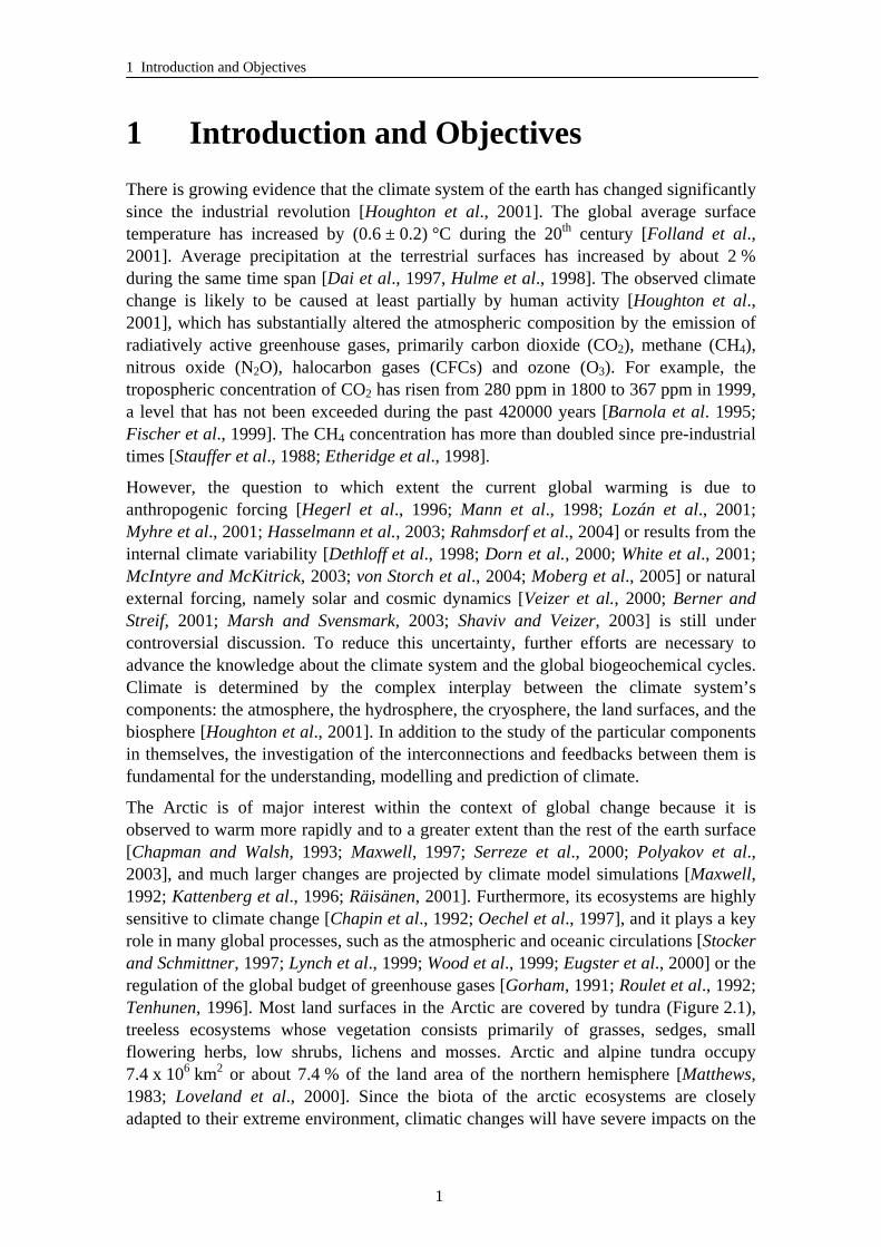
1 Introduction and Objectives There is growing evidence that the climate system of the earth has changed significantly since the industrial revolution [Houghton et al., 2001]. The global average surface temperature has increased by (0.6 ± 0.2) °C during the 20th century [Folland et al., 2001]. Average precipitation at the terrestrial surfaces has increased by about 2 % during the same time span [Dai et al., 1997, Hulme et al., 1998]. The observed climate change is likely to be caused at least partially by human activity [Houghton et al., 2001], which has substantially altered the atmospheric composition by the emission of radiatively active greenhouse gases, primarily carbon dioxide (CO2), methane (CH4), nitrous oxide (N2O), halocarbon gases (CFCs) and ozone (O3). For example, the tropospheric concentration of CO2 has risen from 280 ppm in 1800 to 367 ppm in 1999, a level that has not been exceeded during the past 420000 years [Barnola et al. 1995; Fischer et al., 1999]. The CH4 concentration has more than doubled since pre-industrial times [Stauffer et al., 1988; Etheridge et al., 1998].
However, the question to which extent the current global warming is due to anthropogenic forcing [Hegerl et al., 1996; Mann et al., 1998; Lozán et al., 2001; Myhre et al., 2001; Hasselmann et al., 2003; Rahmsdorf et al., 2004] or results from the internal climate variability [Dethloff et al., 1998; Dorn et al., 2000; White et al., 2001; McIntyre and McKitrick, 2003; von Storch et al., 2004; Moberg et al., 2005] or natural external forcing, namely solar and cosmic dynamics [Veizer et al., 2000; Berner and Streif, 2001; Marsh and Svensmark, 2003; Shaviv and Veizer, 2003] is still under controversial discussion. To reduce this uncertainty, further efforts are necessary to advance the knowledge about the climate system and the global biogeochemical cycles. Climate is determined by the complex interplay between the climate system’s components: the atmosphere, the hydrosphere, the cryosphere, the land surfaces, and the biosphere [Houghton et al., 2001]. In addition to the study of the particular components in themselves, the investigation of the interconnections and feedbacks between them is fundamental for the understanding, modelling and prediction of climate.
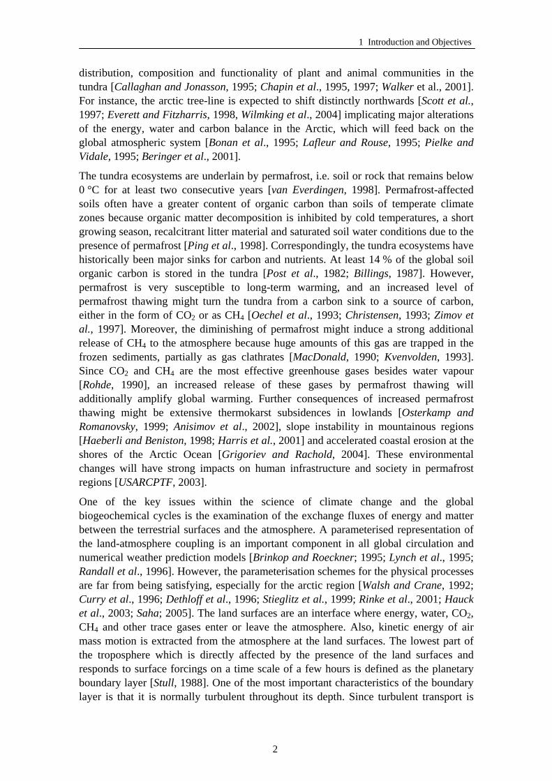
The Arctic is of major interest within the context of global change because it is observed to warm more rapidly and to a greater extent than the rest of the earth surface [Chapman and Walsh, 1993; Maxwell, 1997; Serreze et al., 2000; Polyakov et al., 2003], and much larger changes are projected by climate model simulations [Maxwell, 1992; Kattenberg et al., 1996; Räisänen, 2001]. Furthermore, its ecosystems are highly sensitive to climate change [Chapin et al., 1992; Oechel et al., 1997], and it plays a key role in many global processes, such as the atmospheric and oceanic circulations [Stocker and Schmittner, 1997; Lynch et al., 1999; Wood et al., 1999; Eugster et al., 2000] or the regulation of the global budget of greenhouse gases [Gorham, 1991; Roulet et al., 1992; Tenhunen, 1996]. Most land surfaces in the Arctic are covered by tundra (Figure 2.1), treeless ecosystems whose vegetation consists primarily of grasses, sedges, small flowering herbs, low shrubs, lichens and mosses. Arctic and alpine tundra occupy 7.4 x 10⁶ km2 or about 7.4 % of the land area of the northern hemisphere [Matthews, 1983; Loveland et al., 2000]. Since the biota of the arctic ecosystems are closely adapted to their extreme environment, climatic changes will have severe impacts on the
1
1 Introduction and Objectives
distribution, composition and functionality of plant and animal communities in the tundra [Callaghan and Jonasson, 1995; Chapin et al., 1995, 1997; Walker et al., 2001]. For instance, the arctic tree-line is expected to shift distinctly northwards [Scott et al., 1997; Everett and Fitzharris, 1998, Wilmking et al., 2004] implicating major alterations of the energy, water and carbon balance in the Arctic, which will feed back on the global atmospheric system [Bonan et al., 1995; Lafleur and Rouse, 1995; Pielke and Vidale, 1995; Beringer et al., 2001].
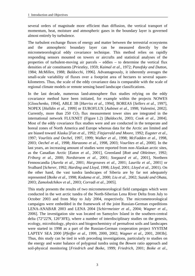
The tundra ecosystems are underlain by permafrost, i.e. soil or rock that remains below 0 °C for at least two consecutive years [van Everdingen, 1998]. Permafrost-affected soils often have a greater content of organic carbon than soils of temperate climate zones because organic matter decomposition is inhibited by cold temperatures, a short growing season, recalcitrant litter material and saturated soil water conditions due to the presence of permafrost [Ping et al., 1998]. Correspondingly, the tundra ecosystems have historically been major sinks for carbon and nutrients. At least 14 % of the global soil organic carbon is stored in the tundra [Post et al., 1982; Billings, 1987]. However, permafrost is very susceptible to long-term warming, and an increased level of permafrost thawing might turn the tundra from a carbon sink to a source of carbon, either in the form of CO2 or as CH4 [Oechel et al., 1993; Christensen, 1993; Zimov et al., 1997]. Moreover, the diminishing of permafrost might induce a strong additional release of CH4 to the atmosphere because huge amounts of this gas are trapped in the frozen sediments, partially as gas clathrates [MacDonald, 1990; Kvenvolden, 1993]. Since CO2 and CH4 are the most effective greenhouse gases besides water vapour [Rohde, 1990], an increased release of these gases by permafrost thawing will additionally amplify global warming. Further consequences of increased permafrost thawing might be extensive thermokarst subsidences in lowlands [Osterkamp and Romanovsky, 1999; Anisimov et al., 2002], slope instability in mountainous regions [Haeberli and Beniston, 1998; Harris et al., 2001] and accelerated coastal erosion at the shores of the Arctic Ocean [Grigoriev and Rachold, 2004]. These environmental changes will have strong impacts on human infrastructure and society in permafrost regions [USARCPTF, 2003].
One of the key issues within the science of climate change and the global biogeochemical cycles is the examination of the exchange fluxes of energy and matter between the terrestrial surfaces and the atmosphere. A parameterised representation of the land-atmosphere coupling is an important component in all global circulation and numerical weather prediction models [Brinkop and Roeckner; 1995; Lynch et al., 1995; Randall et al., 1996]. However, the parameterisation schemes for the physical processes are far from being satisfying, especially for the arctic region [Walsh and Crane, 1992; Curry et al., 1996; Dethloff et al., 1996; Stieglitz et al., 1999; Rinke et al., 2001; Hauck et al., 2003; Saha; 2005]. The land surfaces are an interface where energy, water, CO2, CH4 and other trace gases enter or leave the atmosphere. Also, kinetic energy of air mass motion is extracted from the atmosphere at the land surfaces. The lowest part of the troposphere which is directly affected by the presence of the land surfaces and responds to surface forcings on a time scale of a few hours is defined as the planetary boundary layer [Stull, 1988]. One of the most important characteristics of the boundary layer is that it is normally turbulent throughout its depth. Since turbulent transport is
2
1 Introduction and Objectives
several orders of magnitude more efficient than diffusion, the vertical transport of momentum, heat, moisture and atmospheric gases in the boundary layer is governed almost entirely by turbulence.
The turbulent exchange fluxes of energy and matter between the terrestrial ecosystems and the atmospheric boundary layer can be measured directly by the micrometeorological eddy covariance technique. This method relies on rapidly responding sensors mounted on towers or aircrafts and statistical analyses of the properties of turbulent-moving air parcels – eddies – to determine the vertical flux densities of air constituents [Priestley, 1959; Kaimal et al., 1972; Panofsky and Dutton, 1984; McMillen, 1988; Baldocchi, 1996]. Advantageously, it inherently averages the small-scale variability of fluxes over a footprint area of hectares to several square-kilometres. Thus, the scale of the eddy covariance data is comparable with the scale of regional climate models or remote sensing based landscape classifications.
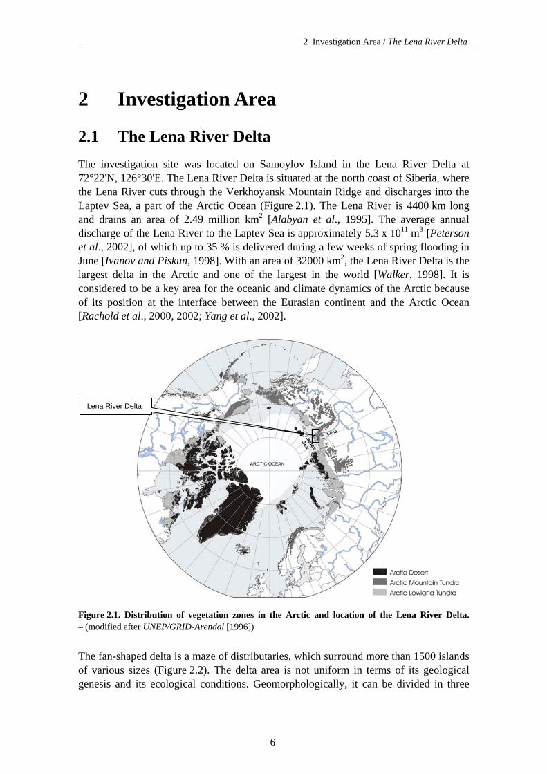
In the last decade, numerous land-atmosphere flux studies relying on the eddy covariance method have been initiated, for example within the projects NOWES [Gloochenko, 1994], ABLE 3B [Harriss et al., 1994], BOREAS [Sellers et al., 1997], NOPEX [Halldin et al., 1999] or EUROFLUX [Aubinet et al., 1998; Valentini, 2002]. Currently, more than 250 CO2 flux measurement tower sites are integrated in the international network FLUXNET (Figure 1.2) [Baldocchi, 2003; Cook et al., 2004]. Most of the eddy covariance flux studies were and are conducted in the temperate and boreal zones of North America and Europe whereas data for the Arctic are limited and are biased toward Alaska [Fan et al., 1992; Fitzjarrald and Moore, 1992; Eugster et al., 1997; Vourlitis and Oechel, 1997, 1999; Walker et al., 1998; McFadden et al., 1998, 2003; Oechel et al., 1998; Harazono et al., 1998, 2003; Vourlites et al., 2000]. In the last years, an increasing amount of studies were reported from non-Alaskan arctic sites, as the Canadian Arctic [Eaton et al., 2001], Greenland [Rott and Obleitner, 1992; Friborg et al., 2000; Nordstroem et al., 2001; Soegaard et al., 2001], Northern Fennoscandia [Aurela et al., 2001; Hargreaves et al., 2001; Laurila et al., 2001] or Svalbard [Scherer, 1992; Harding and Lloyd, 1998; Lloyd, 2001; Lloyd et al., 2001). On the other hand, the vast tundra landscapes of Siberia are by far not adequately represented [Boike et al., 1998; Kodama et al., 2000; Liu et al., 2002; Suzuki and Ohata, 2003; Zamolodchikov et al., 2003; Corradi et al., 2005].
This study presents the results of two micrometeorological field campaigns which were conducted in the wet arctic tundra of the North-Siberian Lena River Delta from July to October 2003 and from May to July 2004, respectively. The micrometeorological campaigns were embedded in the framework of the joint Russian-German expeditions LENA-ANABAR 2003 and LENA 2004 [Schirrmeister et al., 2004; Wagner et al., 2006]. The investigation site was located on Samoylov Island in the southern-central delta (72°22'N, 126°30'E), where a number of interdisciplinary studies on the genesis, ecology, microbiology, physics and biogeochemistry of permafrost soils and landscapes were started in 1998 as a part of the Russian-German cooperation project SYSTEM LAPTEV SEA 2000 [Pfeiffer et al., 1999, 2000, 2002; Wagner et al., 2001, 2003b]. Thus, this study can be tied in with preceding investigations, particularly to studies on the energy and water balance of polygonal tundra using the Bowen ratio approach and soil-physical monitoring [Friedrich and Boike, 1999; Friedrich, 2001; Boike et al.,
3

1 Introduction and Objectives
2003b] and to soil-scientific investigations [Becker et al., 1998; Fiedler et al., 2004; Kutzbach, 2000; Kutzbach et al., 2004a; Pfeiffer et al., 1999, 2002].
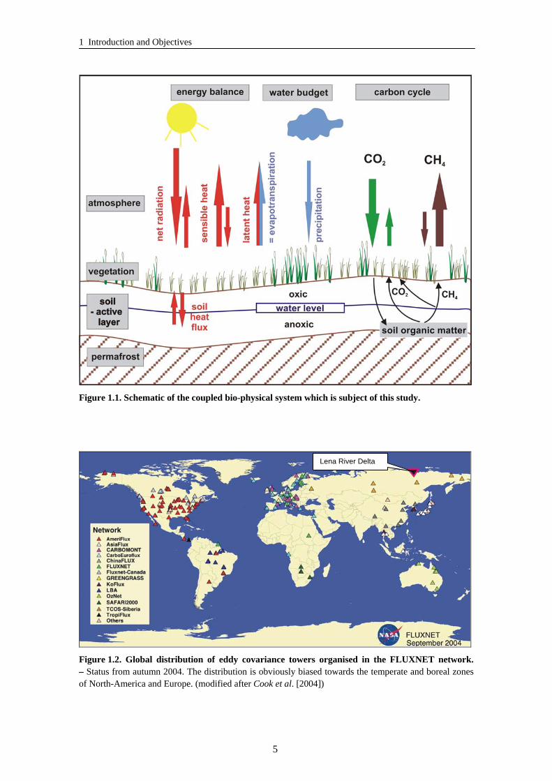
The micrometeorological campaigns described in this work included the investigation of the turbulent fluxes of momentum, energy, water vapour and CO2 by an eddy covariance measurement system (ECS) along with supporting meteorological and soil-meteorological measurements [Kutzbach et al., 2003, 2004b; Wille et al., 2003; 2004; Wille and Boike, 2006]. The study shall contribute to the understanding of the physical and biogeochemical interaction processes between permafrost soils, tundra vegetation and the atmosphere (Figure 1.1), which is necessary for assessing the impact of climate change on arctic tundra ecosystems and the possible feedbacks on the climate system.
In detail, the objectives of the study were to:
• characterise the temporal variations of the exchange fluxes of energy, water and CO2 on diurnal to seasonal time scales at a wet arctic tundra site,
• examine the energy partitioning at the investigated tundra site,
• quantify evapotranspiration, gross photosynthesis, ecosystem respiration and net ecosystem CO2 exchange on the landscape scale,
• investigate the interconnections between the energy balance, the water budget and the CO2 budget at the investigated tundra site,
• provide data for the validation and improvement of process models and parameterisation schemes for climate models,
• analyse the regulation of the exchange fluxes by climatic forcings,
• assess how the exchange fluxes of energy and matter will respond to changes of the arctic climate.
4
1 Introduction and Objectives
Figure 1.1. Schematic of the coupled bio-physical system which is subject of this study.
Lena River Delta
Figure 1.2. Global distribution of eddy covariance towers organised in the FLUXNET network. – Status from autumn 2004. The distribution is obviously biased towards the temperate and boreal zones of North-America and Europe. (modified after Cook et al. [2004])
5
2 Investigation Area / The Lena River Delta
2 Investigation Area
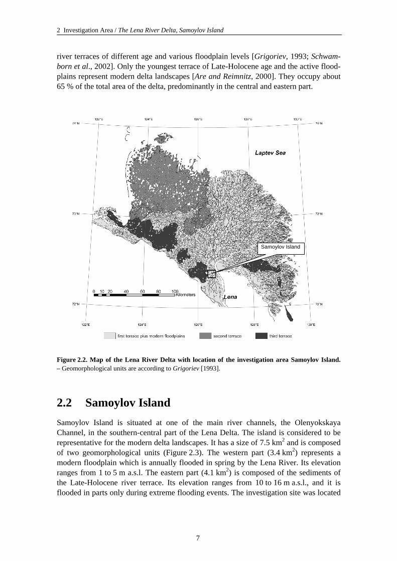
2.1 The Lena River Delta The investigation site was located on Samoylov Island in the Lena River Delta at 72°22'N, 126°30'E. The Lena River Delta is situated at the north coast of Siberia, where the Lena River cuts through the Verkhoyansk Mountain Ridge and discharges into the Laptev Sea, a part of the Arctic Ocean (Figure 2.1). The Lena River is 4400 km long and drains an area of 2.49 million km2 [Alabyan et al., 1995]. The average annual discharge of the Lena River to the Laptev Sea is approximately 5.3 x 10¹¹ m3 [Peterson et al., 2002], of which up to 35 % is delivered during a few weeks of spring flooding in June [Ivanov and Piskun, 1998]. With an area of 32000 km2, the Lena River Delta is the largest delta in the Arctic and one of the largest in the world [Walker, 1998]. It is considered to be a key area for the oceanic and climate dynamics of the Arctic because of its position at the interface between the Eurasian continent and the Arctic Ocean [Rachold et al., 2000, 2002; Yang et al., 2002].
Lena River Delta
Figure 2.1. Distribution of vegetation zones in the Arctic and location of the Lena River Delta. – (modified after UNEP/GRID-Arendal [1996])
The fan-shaped delta is a maze of distributaries, which surround more than 1500 islands of various sizes (Figure 2.2). The delta area is not uniform in terms of its geological genesis and its ecological conditions. Geomorphologically, it can be divided in three
6
2 Investigation Area / The Lena River Delta, Samoylov Island
river terraces of different age and various floodplain levels [Grigoriev, 1993; Schwam-born et al., 2002]. Only the youngest terrace of Late-Holocene age and the active flood-plains represent modern delta landscapes [Are and Reimnitz, 2000]. They occupy about 65 % of the total area of the delta, predominantly in the central and eastern part.
Samoylov Island
Figure 2.2. Map of the Lena River Delta with location of the investigation area Samoylov Island. – Geomorphological units are according to Grigoriev [1993].
2.2 Samoylov Island Samoylov Island is situated at one of the main river channels, the Olenyokskaya Channel, in the southern-central part of the Lena Delta. The island is considered to be representative for the modern delta landscapes. It has a size of 7.5 km2 and is composed of two geomorphological units (Figure 2.3). The western part (3.4 km2) represents a modern floodplain which is annually flooded in spring by the Lena River. Its elevation ranges from 1 to 5 m a.s.l. The eastern part (4.1 km2) is composed of the sediments of the Late-Holocene river terrace. Its elevation ranges from 10 to 16 m a.s.l., and it is flooded in parts only during extreme flooding events. The investigation site was located
7
2 Investigation Area / Samoylov Island
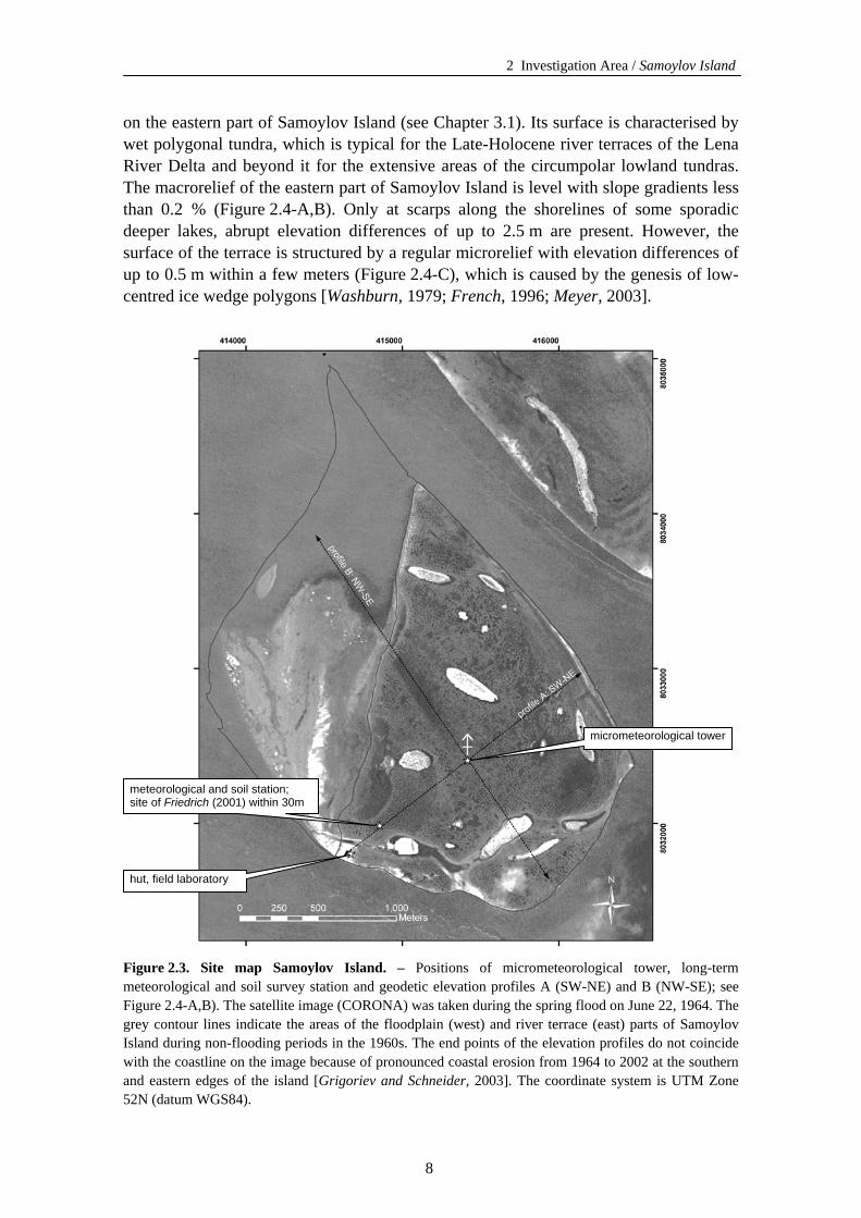
on the eastern part of Samoylov Island (see Chapter 3.1). Its surface is characterised by wet polygonal tundra, which is typical for the Late-Holocene river terraces of the Lena River Delta and beyond it for the extensive areas of the circumpolar lowland tundras. The macrorelief of the eastern part of Samoylov Island is level with slope gradients less than 0.2 % (Figure 2.4-A,B). Only at scarps along the shorelines of some sporadic deeper lakes, abrupt elevation differences of up to 2.5 m are present. However, the surface of the terrace is structured by a regular microrelief with elevation differences of up to 0.5 m within a few meters (Figure 2.4-C), which is caused by the genesis of low-centred ice wedge polygons [Washburn, 1979; French, 1996; Meyer, 2003].
micrometeorological tower
meteorological and soil station; site of Friedrich (2001) within 30m
hut, field laboratory
Figure 2.3. Site map Samoylov Island. – Positions of micrometeorological tower, long-term meteorological and soil survey station and geodetic elevation profiles A (SW-NE) and B (NW-SE); see Figure 2.4-A,B). The satellite image (CORONA) was taken during the spring flood on June 22, 1964. The grey contour lines indicate the areas of the floodplain (west) and river terrace (east) parts of Samoylov Island during non-flooding periods in the 1960s. The end points of the elevation profiles do not coincide with the coastline on the image because of pronounced coastal erosion from 1964 to 2002 at the southern and eastern edges of the island [Grigoriev and Schneider, 2003]. The coordinate system is UTM Zone 52N (datum WGS84).
8
2 Investigation Area / Samoylov Island
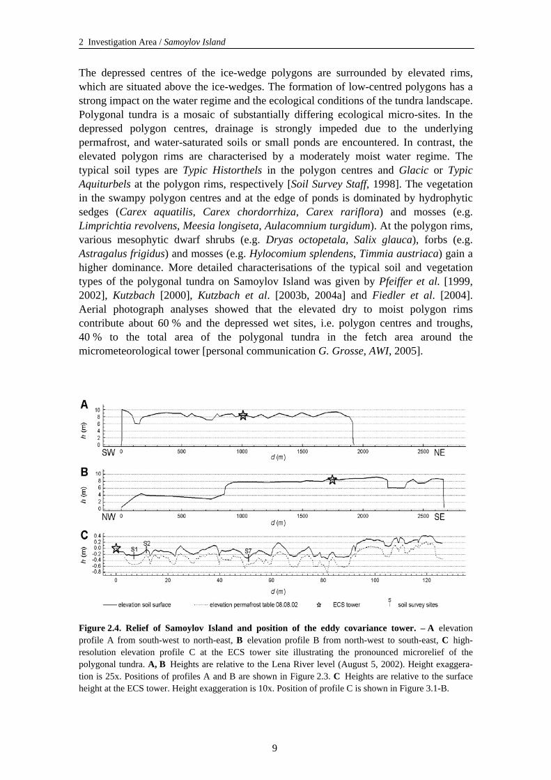
The depressed centres of the ice-wedge polygons are surrounded by elevated rims, which are situated above the ice-wedges. The formation of low-centred polygons has a strong impact on the water regime and the ecological conditions of the tundra landscape. Polygonal tundra is a mosaic of substantially differing ecological micro-sites. In the depressed polygon centres, drainage is strongly impeded due to the underlying permafrost, and water-saturated soils or small ponds are encountered. In contrast, the elevated polygon rims are characterised by a moderately moist water regime. The typical soil types are Typic Historthels in the polygon centres and Glacic or Typic Aquiturbels at the polygon rims, respectively [Soil Survey Staff, 1998]. The vegetation in the swampy polygon centres and at the edge of ponds is dominated by hydrophytic sedges (Carex aquatilis, Carex chordorrhiza, Carex rariflora) and mosses (e.g. Limprichtia revolvens, Meesia longiseta, Aulacomnium turgidum). At the polygon rims, various mesophytic dwarf shrubs (e.g. Dryas octopetala, Salix glauca), forbs (e.g. Astragalus frigidus) and mosses (e.g. Hylocomium splendens, Timmia austriaca) gain a higher dominance. More detailed characterisations of the typical soil and vegetation types of the polygonal tundra on Samoylov Island was given by Pfeiffer et al. [1999, 2002], Kutzbach [2000], Kutzbach et al. [2003b, 2004a] and Fiedler et al. [2004]. Aerial photograph analyses showed that the elevated dry to moist polygon rims contribute about 60 % and the depressed wet sites, i.e. polygon centres and troughs, 40 % to the total area of the polygonal tundra in the fetch area around the micrometeorological tower [personal communication G. Grosse, AWI, 2005].
Figure 2.4. Relief of Samoylov Island and position of the eddy covariance tower. – A elevation profile A from south-west to north-east, B elevation profile B from north-west to south-east, C high-resolution elevation profile C at the ECS tower site illustrating the pronounced microrelief of the polygonal tundra. A, B Heights are relative to the Lena River level (August 5, 2002). Height exaggera-tion is 25x. Positions of profiles A and B are shown in Figure 2.3. C Heights are relative to the surface height at the ECS tower. Height exaggeration is 10x. Position of profile C is shown in Figure 3.1-B.
9
2 Investigation Area / Samoylov Island
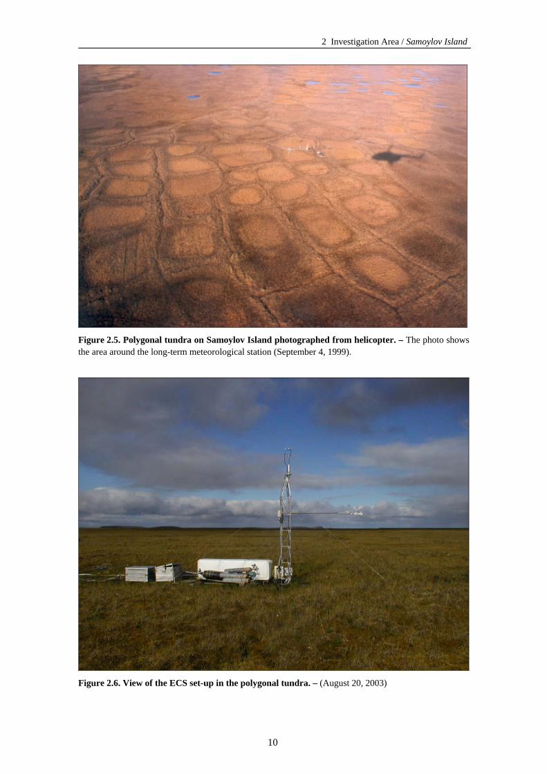
Figure 2.5. Polygonal tundra on Samoylov Island photographed from helicopter. – The photo shows the area around the long-term meteorological station (September 4, 1999).
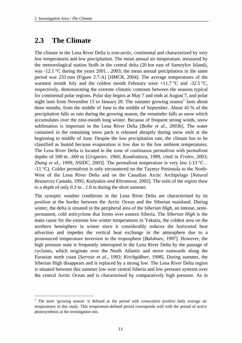
Figure 2.6. View of the ECS set-up in the polygonal tundra. – (August 20, 2003)
10
2 Investigation Area / The Climate
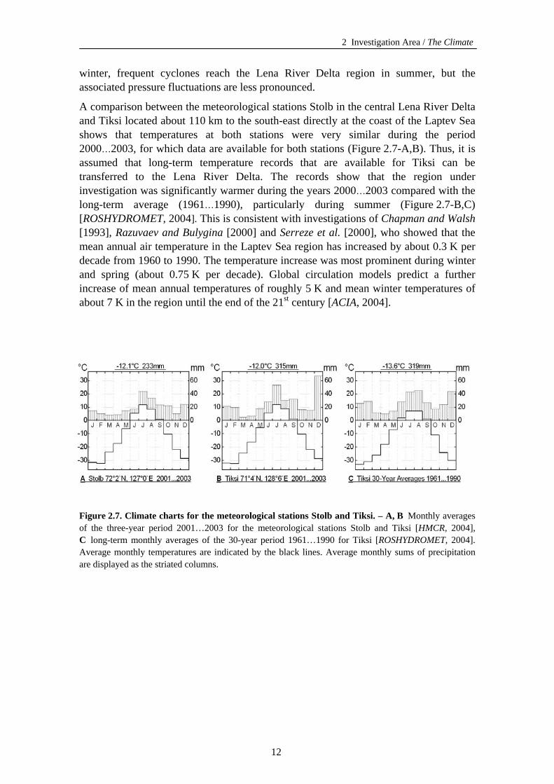
2.3 The Climate The climate in the Lena River Delta is true-arctic, continental and characterized by very low temperatures and low precipitation. The mean annual air temperature, measured by the meteorological station Stolb in the central delta (20 km east of Samoylov Island), was -12.1 °C during the years 2001…2003; the mean annual precipitation in the same period was 233 mm (Figure 2.7-A) [HMCR, 2004]. The average temperatures of the warmest month July and the coldest month February were +11.7 °C and -32.5 °C, respectively, demonstrating the extreme climatic contrasts between the seasons typical for continental polar regions. Polar day begins at May 7 and ends at August 7, and polar night lasts from November 15 to January 28. The summer growing season1 lasts about three months, from the middle of June to the middle of September. About 45 % of the precipitation falls as rain during the growing season, the remainder falls as snow which accumulates over the nine-month long winter. Because of frequent strong winds, snow sublimation is important in the Lena River Delta [Boike et al., 2003b]. The water contained in the remaining snow pack is released abruptly during snow melt at the beginning to middle of June. Despite the low precipitation rate, the climate has to be classified as humid because evaporation is low due to the low ambient temperatures. The Lena River Delta is located in the zone of continuous permafrost with permafrost depths of 500 m…600 m [Grigoriev, 1960; Kondratieva, 1989, cited in Frolov, 2003; Zhang et al., 1999; NSIDC, 2003]. The permafrost temperature is very low (-13 °C… -11 °C). Colder permafrost is only encountered on the Taymyr Peninsula to the North-West of the Lena River Delta and on the Canadian Arctic Archipelago [Natural Resources Canada, 1995; Kotlyakov and Khromova, 2002]. The soils of the region thaw to a depth of only 0.3 m…1.0 m during the short summer.
The synoptic weather conditions in the Lena River Delta are characterised by its position at the border between the Arctic Ocean and the Siberian mainland. During winter, the delta is situated in the peripheral area of the Siberian High, an intense, semi-permanent, cold anticyclone that forms over eastern Siberia. The Siberian High is the main cause for the extreme low winter temperatures in Yakutia, the coldest area on the northern hemisphere in winter since it considerably reduces the horizontal heat advection and impedes the vertical heat exchange in the atmosphere due to a pronounced temperature inversion in the troposphere [Balobaev, 1997]. However, the high pressure state is frequently interrupted in the Lena River Delta by the passage of cyclones, which originate over the North Atlantic and move eastwards along the Eurasian north coast [Serreze et al., 1993; Kirchgäßner, 1998]. During summer, the Siberian High disappears and is replaced by a strong low. The Lena River Delta region is situated between this summer low over central Siberia and low pressure systems over the central Arctic Ocean and is characterised by comparatively high pressure. As in
1 The term ‘growing season’ is defined as the period with consecutive positive daily average air temperatures in this study. This temperature-defined period corresponds well with the period of active photosynthesis at the investigation site.
11
2 Investigation Area / The Climate
winter, frequent cyclones reach the Lena River Delta region in summer, but the associated pressure fluctuations are less pronounced.
A comparison between the meteorological stations Stolb in the central Lena River Delta and Tiksi located about 110 km to the south-east directly at the coast of the Laptev Sea shows that temperatures at both stations were very similar during the period 2000…2003, for which data are available for both stations (Figure 2.7-A,B). Thus, it is assumed that long-term temperature records that are available for Tiksi can be transferred to the Lena River Delta. The records show that the region under investigation was significantly warmer during the years 2000…2003 compared with the long-term average (1961…1990), particularly during summer (Figure 2.7-B,C) [ROSHYDROMET, 2004]. This is consistent with investigations of Chapman and Walsh [1993], Razuvaev and Bulygina [2000] and Serreze et al. [2000], who showed that the mean annual air temperature in the Laptev Sea region has increased by about 0.3 K per decade from 1960 to 1990. The temperature increase was most prominent during winter and spring (about 0.75 K per decade). Global circulation models predict a further increase of mean annual temperatures of roughly 5 K and mean winter temperatures of about 7 K in the region until the end of the 21st century [ACIA, 2004].
Figure 2.7. Climate charts for the meteorological stations Stolb and Tiksi. – A, B Monthly averages of the three-year period 2001…2003 for the meteorological stations Stolb and Tiksi [HMCR, 2004], C long-term monthly averages of the 30-year period 1961…1990 for Tiksi [ROSHYDROMET, 2004]. Average monthly temperatures are indicated by the black lines. Average monthly sums of precipitation are displayed as the striated columns.
12
3 Methods / Eddy Covariance Measurements
3 Methods
3.1 Eddy Covariance Measurements 3.1.1 General Set-Up
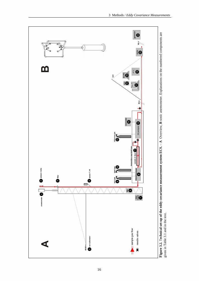
The eddy covariance measurement system (ECS) was established at a central position within the wet polygonal tundra of the eastern part of Samoylov Island (415417E 8032409N, UTM Zone 52, Figure 2.3, Figure 3.1-A). The spatial arrangement of instruments and supporting facilities at the measurement site is shown in Figure 3.1-B. An overview of the complete technical set-up of the ECS is given in Figure 3.2 and Table 3.1. Fluctuations of wind velocity components and sonic temperature were determined with a three-dimensional sonic anemometer (Solent R3, Gill Instruments Ltd., UK). Fluctuations of H2O and CO2 concentrations were measured with a closed-path infrared gas analyser (IRGA; LI-7000, LI-COR Inc., USA). Additionally, the ECS included a CH4 analyser based on tuneable diode laser infrared absorption spectroscopy (TDL; TGA 100, Campbell Scientific Ltd., USA). The sonic anemometer was mounted on top of a 3 m aluminium tower so that the effective measurement height was 3.65 m above ground level. The IRGA and the TDL were installed in a weatherproof, insulated and temperature-regulated case at the base of the tower. The sample air intake equipped with a rain diverter was placed 15 cm apart from the median axis of the sonic anemometer transducer array in direction southwest. Sample air was drawn from the intake through the gas analysers, which were arranged in series in the sample gas line, via a heated sampling tube (5 m long, 6.25 mm inner diameter; Dekabon® 1300/Polyethylen) by a vacuum pump (RB0021, Busch Inc., Germany). The flow rate was 20 dm3 min-1. Under these conditions, turbulent flow was maintained inside the tubing system (Reynolds number ≅ 4880). A 1 µm membrane filter (PTFE, TE37, Schleicher & Schuell, Germany) prevented dust contamination. The filter and a needle valve produced a pressure drop to 850 hPa inside the IRGA and to 75 hPa inside the TDL, respectively. Before entering the TDL, the sample air was dried by a gas dryer relying on the principle of reversed flow (PD-200T-48 SS, Perma Pure Inc., USA). The analogous signals from the fast response sensors were synchronously digitised at a frequency of 20 Hz by the anemometer and transferred to a portable PC housed in a tent 40 m away from the tower. The raw data were logged by the software EdiSol (J. Massheder, University of Edinburgh, UK) and were archived on hard-disc for subsequent post-processing of turbulent fluxes and micrometeorological parameters.
A diesel generator (100 m away from the tower) and an uninterruptible power supply (near to the tent) ensured autonomous and continuous operation. Wooden boardwalks connected all parts of the system to reduce disturbance of the swampy tundra soils and the vegetation. To minimise perturbation of the aerodynamic flow field and the micrometeorological measurements, all devices were set up in a line to the southwest from the tower, which was the least-frequent wind direction during the previous summers. Data gathered during periods when winds were coming from directions
13
3 Methods / Eddy Covariance Measurements
ranging between 230° and 270° were excluded from further analyses because of the possible disturbance by the generator.
A
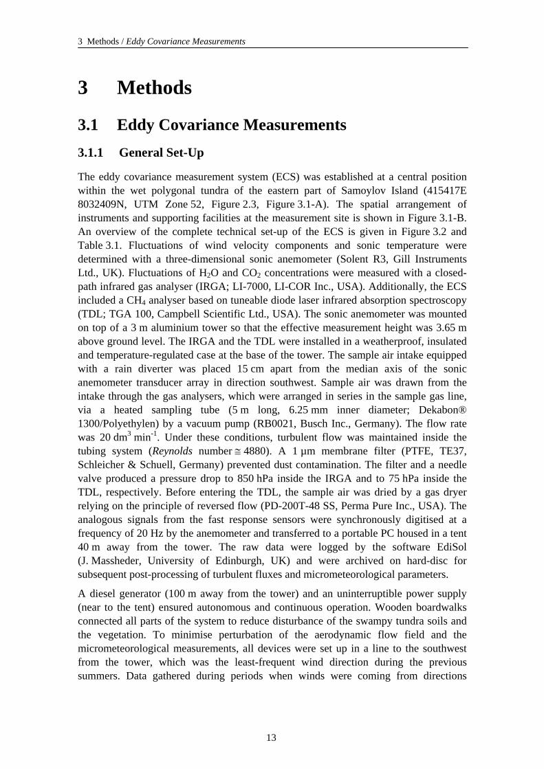
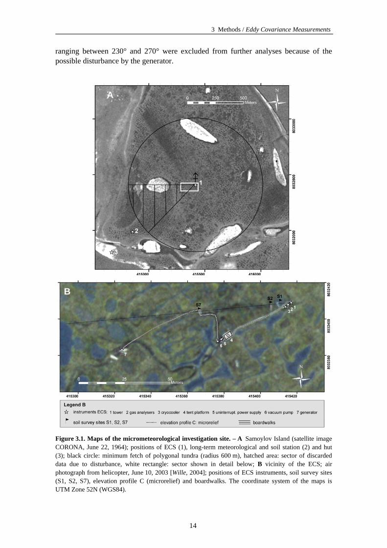
B
Figure 3.1. Maps of the micrometeorological investigation site. – A Samoylov Island (satellite image CORONA, June 22, 1964); positions of ECS (1), long-term meteorological and soil station (2) and hut (3); black circle: minimum fetch of polygonal tundra (radius 600 m), hatched area: sector of discarded data due to disturbance, white rectangle: sector shown in detail below; B vicinity of the ECS; air photograph from helicopter, June 10, 2003 [Wille, 2004]; positions of ECS instruments, soil survey sites (S1, S2, S7), elevation profile C (microrelief) and boardwalks. The coordinate system of the maps is UTM Zone 52N (WGS84).
14
3 Methods / Eddy Covariance Measurements
Wet polygonal tundra extended at least 600 m in all directions from the ECS tower (Figure 3.1-A). To satisfy the fetch requirements of the eddy covariance method, a measurement height of 3.65 m above ground level was chosen. Thus, the rule of thumb was observed that the height for eddy covariance measurements should be less than about one-hundredth of the distance of the upwind uniform terrain [McMillen, 1988; Garrat, 1990; Stannard, 1997]. A more elaborate footprint analysis following Schuepp et al. [1990] assessed the 80 % cumulative footprint, i.e. the upwind distance within which 80 % of the observed flux values originated, to be on average (457 ± 93) m during the snow-free periods. During 96.5 % of the snow-free periods, the 80 % cumulative footprint was within 600 m. However, the 80 % cumulative footprint increased to an average of (781 ± 138) m during the periods when snow covered the surface. Detailed results of the footprint analysis are shown in Chapter 4. At the periphery of the 600 m radius circle around the tower, several larger lakes interrupt the homogeneity of the polygonal tundra fetch. Given the long distance between the lakes and the tower, the inhomogeneity error introduced to the flux estimates for polygonal tundra by the lakes is assessed to be at maximum 5 % during snow-free periods.
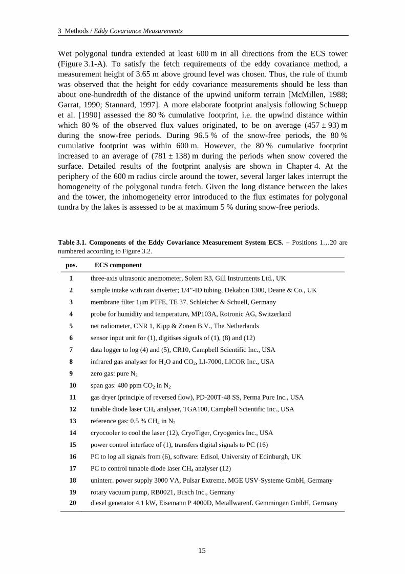
Table 3.1. Components of the Eddy Covariance Measurement System ECS. – Positions 1…20 are numbered according to Figure 3.2.
pos. ECS component
1 three-axis ultrasonic anemometer, Solent R3, Gill Instruments Ltd., UK
2 sample intake with rain diverter; 1/4”-ID tubing, Dekabon 1300, Deane & Co., UK
3 membrane filter 1μm PTFE, TE 37, Schleicher & Schuell, Germany
4 probe for humidity and temperature, MP103A, Rotronic AG, Switzerland
5 net radiometer, CNR 1, Kipp & Zonen B.V., The Netherlands
6 sensor input unit for (1), digitises signals of (1), (8) and (12)
7 data logger to log (4) and (5), CR10, Campbell Scientific Inc., USA
8 infrared gas analyser for H2O and CO2, LI-7000, LICOR Inc., USA
9 zero gas: pure N2
10 span gas: 480 ppm CO2 in N2
11 gas dryer (principle of reversed flow), PD-200T-48 SS, Perma Pure Inc., USA
12 tunable diode laser CH4 analyser, TGA100, Campbell Scientific Inc., USA
13 reference gas: 0.5 % CH4 in N2
14 cryocooler to cool the laser (12), CryoTiger, Cryogenics Inc., USA
15 power control interface of (1), transfers digital signals to PC (16)
16 PC to log all signals from (6), software: Edisol, University of Edinburgh, UK
17 PC to control tunable diode laser CH4 analyser (12)
18 uninterr. power supply 3000 VA, Pulsar Extreme, MGE USV-Systeme GmbH, Germany
19 rotary vacuum pump, RB0021, Busch Inc., Germany 20 diesel generator 4.1 kW, Eisemann P 4000D, Metallwarenf. Gemmingen GmbH, Germany
15
3 Methods / Eddy Covariance Measurements
Figu
re 3
.2. T
echn
ical
set-
up o
f the
edd
y co
vari
ance
mea
sure
men
t sys
tem
EC
S. –
A O
verv
iew
, B so
nic
anem
omet
er. E
xpla
natio
ns o
n th
e nu
mbe
red
com
pone
nts a
re
give
n in
Tab
le 3
.1 a
nd in
the
text
.
16

3 Methods / Eddy Covariance Measurements
3.1.2 The Sonic Anemometer
The sonic anemometer measures wind speed and the still air speed of sound on three non-orthogonal axes. From these measurements, orthogonal wind speed components and sonic temperature is computed. The sonic anemometer consists of three transducer pairs (Figure 3.2-B). Each transducer can serve alternately as transmitter and receiver. Group velocity, i.e. the velocity at which sound travels through air relative to a stationary observer, is the vector sum of the still air speed of sound and the velocity of air that supports the acoustic waves. Thus, measuring the time of flight of sonic impulses between the two transducers of known separation in both directions allows for determining the speed of the moving air mass along the axis that connects the transducers. The wind speed ui along any axis i can be found by:
⎥⎦
⎤⎢⎣
⎡−=
biai
ii tt
du 11
2 , (1)
where di is the distance between the transducers of the respective axis i, tai is the time of flight of the first sound impulse along the transducer axis i in one direction, tbi is the time of flight of the second sound signal in the opposite direction. The non-orthogonal wind speed components u1, u2, u3 are then transformed into the orthogonal wind speed components u, v, w by a coordinate transformation that is specific for the individual geometry of each anemometer. The errors due to wind blowing normal to the sonic path are corrected on-line before the transformation into orthogonal coordinates.
The sonically determined still air speed of sound vs is the average of the three axes and is determined as follows:
3
112
3
1∑
=⎥⎦
⎤⎢⎣
⎡+
= i biai
i
s
ttd
v , (2)
The sonic temperature Tson can be determined using the dependency of the still air speed of sound on air temperature and specific humidity q:
sonddairdds TRqTRv κκ =+= )513.01(2 , (3)
where κd is the adiabatic exponent, i.e. the ratio of specific heat of dry air at constant pressure to that at constant volume, Rd is the gas constant for dry air. Consequently, the sonic temperature is calculated as:
dd
Sson R
vT
κ
2
= . (4)
Under normal atmospheric conditions which occurred during the campaigns (Tair: -30…+30 °C, q: 0.03…2.5 %) Tson is a good approximation of the virtual temperature Tv:
17
3 Methods / Eddy Covariance Measurements
( ) ( )qTqqTqTT sonsonairv 095.01
513.01608.01608.01 +≅
++
=+= . (5)
The precision of the wind speed measurements measured as RMS noise is ± 1 %. The accuracy of the Tson measurement is ± 0.5 % at 20 °C [Gill Instruments Ltd., 2002].
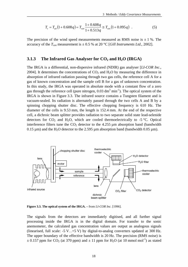
3.1.3 The Infrared Gas Analyser for CO2 and H2O (IRGA)
The IRGA is a differential, non-dispersive infrared (NDIR) gas analyser [LI-COR Inc., 2004]. It determines the concentrations of CO2 and H2O by measuring the difference in absorption of infrared radiation passing through two gas cells, the reference cell A for a gas of known concentration and the sample cell B for a gas of unknown concentration. In this study, the IRGA was operated in absolute mode with a constant flow of a zero gas through the reference cell (pure nitrogen, 0.03 dm3 min-1). The optical system of the IRGA is shown in Figure 3.3. The infrared source contains a Tungsten filament and is vacuum-sealed. Its radiation is alternately passed through the two cells A and B by a spinning chopping shutter disc. The effective chopping frequency is 610 Hz. The diameter of the cells is 9.53 mm, the length is 152.4 mm. At the end of the respective cell, a dichroic beam splitter provides radiation to two separate solid state lead-selenide detectors for CO2 and H2O, which are cooled thermoelectrically to -5 °C. Optical interference filters tune the CO2 detector to the 4.255 µm absorption band (bandwidth 0.15 µm) and the H2O detector to the 2.595 µm absorption band (bandwidth 0.05 µm).
Figure 3.3. The optical system of the IRGA. – from LI-COR Inc. [1996].
The signals from the detectors are immediately digitised, and all further signal processing inside the IRGA is in the digital domain. For transfer to the sonic anemometer, the calculated gas concentration values are output as analogous signals (linearised, full scale: -5 V…+5 V) by digital-to-analog converters updated at 300 Hz. The upper boundary of the effective bandwidth is 20 Hz. The precision (RMS noise) is ± 0.157 ppm for CO2 (at 370 ppm) and ± 11 ppm for H2O (at 10 mmol mol-1) as stated
18
3 Methods / Eddy Covariance Measurements
by LI-COR, Inc. [2004]. The accuracy is normally ± 1 % for measurements of CO2 and H2O.
The calculation of volumetric concentrations ciB of the gases i in the sample air is based on the non-linear relationship between absorptance of light at the gas-specific absorption band aiB and the gas concentration in the sample cell B as follows:
⎟⎟⎠
⎞⎜⎜⎝
⎛= i
B
iBiBiB S
pa
fTc , (6)
where TB and pB BB indicate temperature (in °C) and pressure measured continuously by built-in sensors in the sample cell. fi is a third-order polynom for H2O and a fifth-order polynom for CO2, respectively, whose coefficients were empirically determined during factory calibration. Si is a span adjustment factor. The absorptance aiB of a gas i in the sample cell B is defined as:
0
11i
iBiBiB I
Ia −=−= τ , (7)
where τi is transmittance, I0 is the initial light intensity before absorption, and IiA is the resulting light intensity after absorption in the sample cell. If the concentration in the reference cell A is zero, Equation (7) can be rewritten as:
iiA
iB
i
iBiB Z
II
II
a −=−= 110
, (8)
where IiA is light intensity after passing the reference cell A purged with the zero gas. Zi is an offset adjustment factor, which was determined for CO2 and H2O during the weekly user calibration by flushing the sample cell B with the zero gas.
The span adjustment factor Si was set for CO2 during the weekly user calibration by flushing the sample cell B with a reference gas of known CO2 concentration (400 ppm…450 ppm CO2 in pure nitrogen). For H2O, Si was not altered during the campaigns but corrected and applied to the data during post-processing by referencing the span of the H2O signal of the IRGA to measurements of relative humidity RH, air pressure p and air temperature Tair by slow-response meteorological probes (Chapter 3.2) as:
⎟⎟⎠
⎞⎜⎜⎝
⎛
⎟⎟⎠
⎞⎜⎜⎝
⎛
∗∗
=−−
−
B
origOH
orig
B
B
SB
corr
Tc
fSp
TpeRH
fpS
21
1
, (9)
where eS is saturation water vapour pressure determined as a function of Tair [Buck, 1981]. Sorig and Scorr are the original and corrected values for Si, respectively. cH2O-orig denotes the uncorrected H2O concentration data (20 Hz). The overbars indicate time
19
3 Methods / Eddy Covariance Measurements
averaging over 30 min intervals. A detailed deduction of Equation (9) is given in the appendix A1.
3.1.4 Processing of Eddy Covariance Fluxes
Turbulent fluxes and micrometeorological parameters were determined from July 20 to October 22, 2003 (94 complete days), and from May 28 to July 20, 2004 (53 complete days). The time base for all data is YAKT (Yakutsk Time), approximately 0.5 hours ahead of local solar time. The sign convention of this study is that all fluxes are positive when directed away from the ground surface2, both downwards and upwards [Foken, 2003].
Turbulent fluxes were calculated by the eddy covariance method over 30 min averaging intervals using the software EdiRe (Version 1.4.3.987, R. Clement, University of Edinburgh, UK). The processing of the raw data included the following steps:
(a) The concentration signals ci of a gas i were converted to absolute density signals ρi as:
air
iii TR
pMc=ρ , (10)
where Mi is the molecular weight of the gas i, Tair is air temperature, p is air pressure, and R is the universal gas constant.
(b) The records of sonic temperature Tson and the gas densities ρi were detrended using a digital recursive high-pass filter. The filter was similar to that described by McMillen [1988] and can be written:
( ) iii xyy δδ −+= − 11 , (11)
where xi is the original datum at time ti, yi is the low-pass filtered datum at ti, and δ is the weight defined by:
τδ Δ−= e2 , (12)
where Δ is the measurement interval and τ the time constant of the filter. The high-pass filtered signal x' is then calculated as:
iii yxx −=′ . (13)
For Tson, ρH2O and ρCO2, τ was set to 300 s.
2 The ground surface is defined in this study as the idealised interface plane between soil and vegetation on the one side and the atmospheric boundary layer on the other side as it is convenient in micrometeorology. In contrast to the soil-scientific concept, moss and snow layers are defined to be below the ground surface.
20
3 Methods / Eddy Covariance Measurements
(c) The wind components measured by the sonic anemometer were mathematically rotated so that the mean transverse velocity v , the mean vertical velocity w , and the covariance of the transverse and vertical velocities wv ′′ were reduced to zero for each 30 min interval [McMillen, 1988; Aubinet et al., 2000]. Thus, the calculated fluxes were aligned normal to the mean wind streamlines.
(d) The turbulent momentum flux UW was calculated as the covariance of the horizontal with the vertical wind velocity as:
wuUW ′′= , (14)
where u is the horizontal and w the vertical wind speed after coordinate rotation. The primes indicate the fluctuation about the mean and the overbar represents the mean over the sampling interval. The friction velocity u* is given by:
wuu ′′=∗ . (15)
The turbulent fluxes of the scalar quantities sensible heat QH, latent heat QE and CO2 FCO2 were computed as the covariance of the scalar with the vertical wind as follows:
( ) ′′+= wTCCQ sonvOHadadH 2ρρ , (16)
′′= wQ OHE 2ρλ , (17)
′′= wF COCO 22 ρ , (18)
where ρad is density of dry air, ρH2O is density of water vapour in the air, Cad is the specific heat capacity of dry air, Cv is the specific heat capacity of water vapour in the air, and λ is the latent heat of vaporisation. Tson, ρH2O, and ρCO2 are the detrended sonic temperature and gas density signals, respectively. The lag times of the gas density signals with respect to the wind and temperature signals were determined by maximising the covariance of the vertical wind and the gas density signals. The median values of lag time were 0.65 s for H2O and 0.55 s for CO2.
(e) QH was corrected for the effect of moisture on the temperature measurements by the sonic anemometer according to Schotanus et al. [1983]. The correction compensates the difference between Tson and the actual temperature Tair. Thus, the corrected QH can be written as:
( ) ′′+≅ wTCCQ airvOHadadH 2ρρ . (19)
(f) Transfer functions were applied to the turbulent fluxes to account for the imperfect spectral response of the gas analysers, the frequency response of the data acquisition system and the individual sensors, the separation of the sensors, the damping effect of the gas sampling tube and the detrending filter [Moore, 1986; Moncrieff et al., 1997].
21
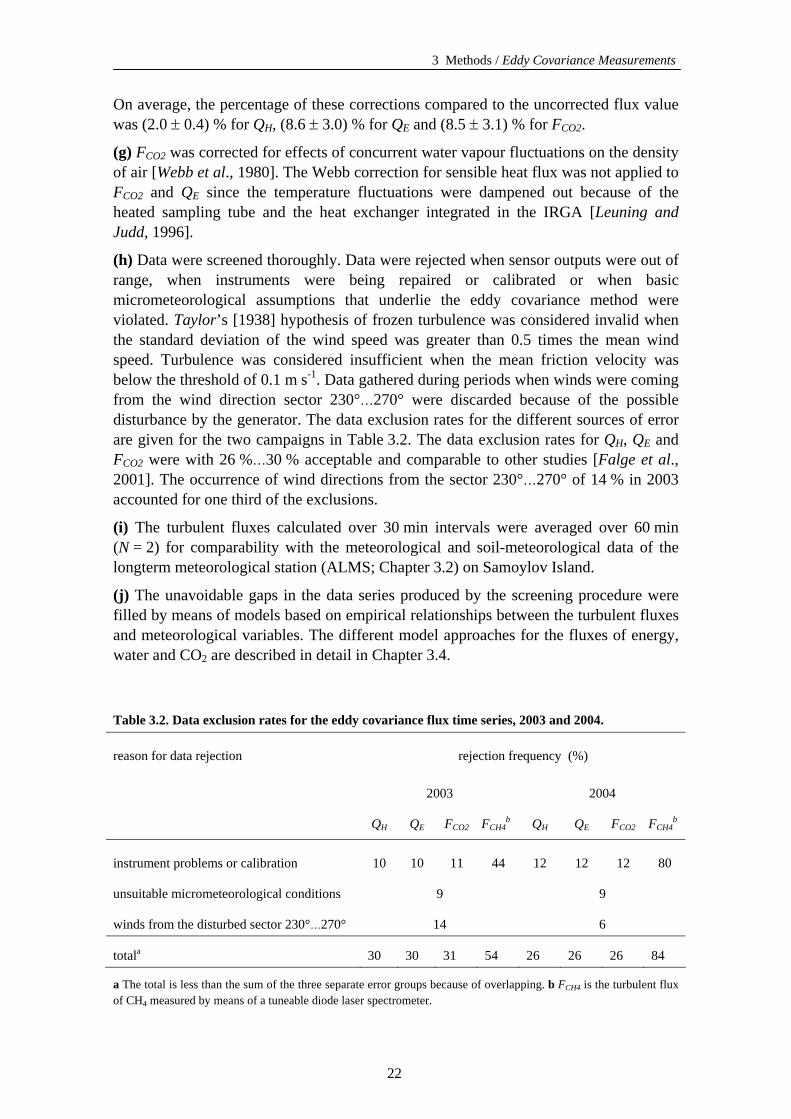
3 Methods / Eddy Covariance Measurements
On average, the percentage of these corrections compared to the uncorrected flux value was (2.0 ± 0.4) % for QH, (8.6 ± 3.0) % for QE and (8.5 ± 3.1) % for FCO2.
(g) FCO2 was corrected for effects of concurrent water vapour fluctuations on the density of air [Webb et al., 1980]. The Webb correction for sensible heat flux was not applied to FCO2 and QE since the temperature fluctuations were dampened out because of the heated sampling tube and the heat exchanger integrated in the IRGA [Leuning and Judd, 1996].
(h) Data were screened thoroughly. Data were rejected when sensor outputs were out of range, when instruments were being repaired or calibrated or when basic micrometeorological assumptions that underlie the eddy covariance method were violated. Taylor’s [1938] hypothesis of frozen turbulence was considered invalid when the standard deviation of the wind speed was greater than 0.5 times the mean wind speed. Turbulence was considered insufficient when the mean friction velocity was below the threshold of 0.1 m s-1. Data gathered during periods when winds were coming from the wind direction sector 230°…270° were discarded because of the possible disturbance by the generator. The data exclusion rates for the different sources of error are given for the two campaigns in Table 3.2. The data exclusion rates for QH, QE and FCO2 were with 26 %…30 % acceptable and comparable to other studies [Falge et al., 2001]. The occurrence of wind directions from the sector 230°…270° of 14 % in 2003 accounted for one third of the exclusions.
(i) The turbulent fluxes calculated over 30 min intervals were averaged over 60 min (N = 2) for comparability with the meteorological and soil-meteorological data of the longterm meteorological station (ALMS; Chapter 3.2) on Samoylov Island.
(j) The unavoidable gaps in the data series produced by the screening procedure were filled by means of models based on empirical relationships between the turbulent fluxes and meteorological variables. The different model approaches for the fluxes of energy, water and CO2 are described in detail in Chapter 3.4.
Table 3.2. Data exclusion rates for the eddy covariance flux time series, 2003 and 2004.
reason for data rejection rejection frequency (%)
2003 2004
QH QE FCO2 FCH4b QH QE FCO2 FCH4
b
instrument problems or calibration 10 10 11 44 12 12 12 80
unsuitable micrometeorological conditions 9 9
winds from the disturbed sector 230°…270° 14 6
totala 30 30 31 54 26 26 26 84
a The total is less than the sum of the three separate error groups because of overlapping. b FCH4 is the turbulent flux of CH4 measured by means of a tuneable diode laser spectrometer.
22
3 Methods / Supporting Meteorological Measurements
3.2 Supporting Meteorological Measurements In addition to the fast-response eddy covariance measurements, a set of supporting slow-response meteorological measurements were conducted. The meteorological data were partly recorded at the ECS tower site and partly provided by an automatic longterm meteorological station (ALMS), which is located 700 m away from the ECS site in the polygonal tundra of Samoylov Island (Figure 2.3, Figure 3.1-A). The ALMS is operated since 1998 by the Alfred Wegener Institute [Friedrich and Boike, 1999; Wille et al. 2003] and was used for previous investigations of the energy and water budget of tundra soils [Friedrich, 2001; Boike et al., 2003b]. The ALMS meteorological measurements used in this study are unpublished data provided by Dr. Julia Boike [Boike, 2005]. An overview of all meteorological measurements used in this study is given in Table 3.3.
The following measurements were integrated in the ECS and were conducted only during the micrometeorological campaigns (Figure 3.2-A, Table 3.1, Table 3.3): Air temperature Tair-A
3 and relative humidity RHA were measured by a shielded meteorological probe (MP103A, ROTRONIC AG, Switzerland) mounted on the ECS tower at a height of 2 m above ground level. Incoming and surface-reflected shortwave and longwave infrared radiation (S↓, S↑, L↓, L↑A) were measured by a net radiometer consisting of two pyranometers and two pyrgeometers (CNR1, Kipp & Zonen B.V., The Netherlands). The net radiometer was installed at the end of a 2 m long cross-arm mounted on the tower at a height of 2 m. Air pressure p was determined with a barometric pressure sensor (RPT410, Druck Messtechnik GmbH, Germany). For comparison with long-term data of the meteorological Station Stolb, the barometric pressure was corrected to sea-level conditions by
10
TRgMh
epp = , (20)
where p and p0 are the actual and the corrected barometric pressure, respectively. h is measurement height above sea level, M molecular weight of dry air (28.9 g mol-1), g is gravity acceleration, R is the universal gas constant and T1 is the approximated temperature midway between h and sea level.
The outputs from the meteorological sensors were recorded every 10 s and averaged over 15 min periods by a data logger (CR10, Campbell Scientific Inc., USA). In 2003, air temperature and relative humidity were recorded by the sonic anemometer at 20 Hz.
The following meteorological data were provided by the ALMS: Liquid precipitation PRl (i.e. rainfall) was recorded with a tipping bucket rain gauge (model 52203, R.M. Young Company, USA). Snow height hsnow was determined with a sonic ranging sensor (SR 50, Campbell Scientific Inc., USA) at a polygon centre. Horizontal wind speed ūB and direction WD
B
BB
were measured by a propeller anemometer at 3 m height (type
3 The subscript A is used to indicate variables that were measured by the ECS when measured also by the ALMS, which is then indicated by the subscript B.
23
3 Methods / Supporting Meteorological Measurements
05103, R.M. Young Company, USA). Air temperatures Tair-0.5m, Tair-B and relative humidity RH
B
BB were measured at 0.5 m and 2 m height by shielded meteorological probes (MP340, ROTRONIC AG, Switzerland). Net radiation Qs* was measured by a net radiometer (NR-Lite, Kipp & Zonen B.V., The Netherlands) installed at a height of 1.35 m. Net radiation readings were corrected for wind speed sensitivity according to Brotzge and Duchon [2000] as recommended by Campbell Scientific Inc. [2003]. The wind speed at the radiometer installation height was estimated from ūB at 3 m and u* (from the ECS) assuming a logarithmic wind profile. Surface longwave radiation L↑
B
BB was measured by a pyrgeometer (CG1, Kipp & Zonen B.V., The Netherlands). The surface radiative temperature Tsur was calculated from L↑B by inverting the Stefan-Boltzmann law [Stefan, 1879; Boltzmann, 1884]:
B
41
81067.5 ⎟⎟⎠
⎞⎜⎜⎝
⎛×
↑=
−εB
sur
LT , (21)
where the emissivity ε was assumed to be 0.98.
The sensors were sampled every 20 s, and hourly averages were stored. The ALMS worked throughout the whole year, thus its data could be used to model the turbulent fluxes over the whole year using the data from the eddy covariance campaigns for model calibration.
Solid precipitation PRs fallen as snow was not measured by the meteorological station on Samoylov Island but was taken from the Russian meteorological station Stolb, which is located about 20 km to the east of Samoylov Island [HMCR, 2004] (see also Chapter 2).
24
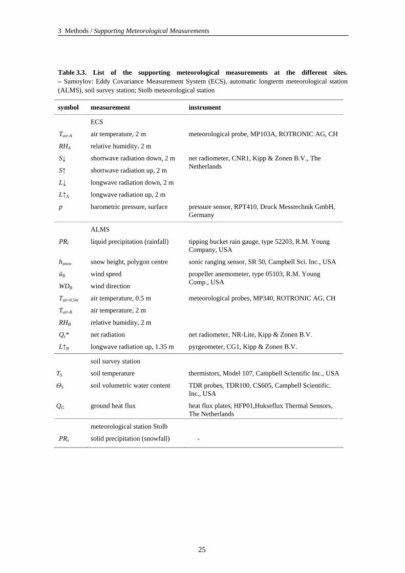
3 Methods / Supporting Meteorological Measurements
Table 3.3. List of the supporting meteorological measurements at the different sites. – Samoylov: Eddy Covariance Measurement System (ECS), automatic longterm meteorological station (ALMS), soil survey station; Stolb meteorological station
symbol measurement instrument
ECS
Tair-A air temperature, 2 m
RHA relative humidity, 2 m
meteorological probe, MP103A, ROTRONIC AG, CH
S↓ shortwave radiation down, 2 m
S↑ shortwave radiation up, 2 m
L↓ longwave radiation down, 2 m
L↑A longwave radiation up, 2 m
net radiometer, CNR1, Kipp & Zonen B.V., The Netherlands
p barometric pressure, surface pressure sensor, RPT410, Druck Messtechnik GmbH, Germany
ALMS
PRl liquid precipitation (rainfall) tipping bucket rain gauge, type 52203, R.M. Young Company, USA
hsnow snow height, polygon centre sonic ranging sensor, SR 50, Campbell Sci. Inc., USA
ūB wind speed
WDB wind direction
propeller anemometer, type 05103, R.M. Young Comp., USA
Tair-0.5m air temperature, 0.5 m
Tair-B air temperature, 2 m
RHB relative humidity, 2 m
meteorological probes, MP340, ROTRONIC AG, CH
Qs* net radiation net radiometer, NR-Lite, Kipp & Zonen B.V.
L↑B longwave radiation up, 1.35 m pyrgeometer, CG1, Kipp & Zonen B.V.
soil survey station
TS soil temperature thermistors, Model 107, Campbell Scientific Inc., USA
ӨS soil volumetric water content TDR probes, TDR100, CS605, Campbell Scientific. Inc., USA
QG ground heat flux heat flux plates, HFP01,Hukseflux Thermal Sensors, The Netherlands
meteorological station Stolb
PRs solid precipitation (snowfall) -
25
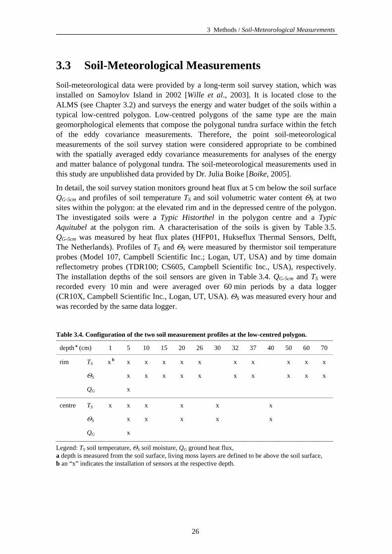
3 Methods / Soil-Meteorological Measurements
3.3 Soil-Meteorological Measurements Soil-meteorological data were provided by a long-term soil survey station, which was installed on Samoylov Island in 2002 [Wille et al., 2003]. It is located close to the ALMS (see Chapter 3.2) and surveys the energy and water budget of the soils within a typical low-centred polygon. Low-centred polygons of the same type are the main geomorphological elements that compose the polygonal tundra surface within the fetch of the eddy covariance measurements. Therefore, the point soil-meteorological measurements of the soil survey station were considered appropriate to be combined with the spatially averaged eddy covariance measurements for analyses of the energy and matter balance of polygonal tundra. The soil-meteorological measurements used in this study are unpublished data provided by Dr. Julia Boike [Boike, 2005].
In detail, the soil survey station monitors ground heat flux at 5 cm below the soil surface QG-5cm and profiles of soil temperature TS and soil volumetric water content ΘS at two sites within the polygon: at the elevated rim and in the depressed centre of the polygon. The investigated soils were a Typic Historthel in the polygon centre and a Typic Aquitubel at the polygon rim. A characterisation of the soils is given by Table 3.5. QG-5cm was measured by heat flux plates (HFP01, Hukseflux Thermal Sensors, Delft, The Netherlands). Profiles of TS and ΘS were measured by thermistor soil temperature probes (Model 107, Campbell Scientific Inc.; Logan, UT, USA) and by time domain reflectometry probes (TDR100; CS605, Campbell Scientific Inc., USA), respectively. The installation depths of the soil sensors are given in Table 3.4. QG-5cm and TS were recorded every 10 min and were averaged over 60 min periods by a data logger (CR10X, Campbell Scientific Inc., Logan, UT, USA). ΘS was measured every hour and was recorded by the same data logger.
Table 3.4. Configuration of the two soil measurement profiles at the low-centred polygon.
depth a (cm) 1 5 10 15 20 26 30 32 37 40 50 60 70
rim TS x b x x x x x x x x x x
ΘS x x x x x x x x x x
QG x
centre TS x x x x x x
ΘS x x x x x
QG x
Legend: TS soil temperature, ΘS soil moisture, QG ground heat flux, a depth is measured from the soil surface, living moss layers are defined to be above the soil surface, b an “x” indicates the installation of sensors at the respective depth.
26
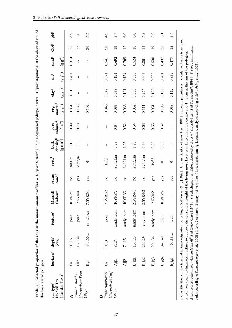
3 Methods / Soil-Meteorological Measurements
pHg
4.9
5.0
5.5
4.9
5.7
6.0
6.0
5.9
5.6
5.1
5.4
C/N
g
31
32
36
50
19
15
16
18
19
21
15
sand
g
(g
g-1
)
0.31
4
--
--
0.54
1
0.69
2
0.70
9
0.52
4
0.28
1
0.53
0
0.43
7
0.47
7
siltg
(g g
-1)
0.20
4
--
--
0.07
1
0.19
1
0.15
4
0.35
5
0.34
3
0.22
6
0.28
1
0.35
9
clay
g
(g
g-1
)
13.1
--
--
0.04
2
0.05
3
0.10
1
0.06
8
0.26
5
0.18
3
0.18
0
0.11
2
org.
m
atte
rg
(g g
-1)
0.35
1
0.13
8
0.10
2
0.34
6
0.06
5
0.03
6
0.05
2
0.11
1
0.06
1
0.10
3
0.05
3
pore
vo
lum
eg (m
3 m-3
)
0.99
0.78
--
--
0.64
0.52
0.54
0.68
0.65
0.67
--
bulk
de
nsity
g
(g c
m-3
)
0.1
0.65
--
--
0.96
1.25
1.25
0.88
0.95
0.86
--
root
sf
3vf,f
,m,
2vf,f
,m
0
1vf,f
3vf,2
f,m
3vf,2
f,m
2vf,f
,1m
2vf,f
,1m
1vf,f
0 0
redu
c.
cond
.e
no
yes
yes
no
no
no
no
no
yes
yes
yes
Mun
sell
Col
ourd
10Y
R2/
3
2.5Y
4/4
7.5Y
R5/
1
7.5Y
R2/
2
10Y
R3/
2
10Y
R3/
2
2.5Y
R4/
1
2.5Y
R4/
2
2.5Y
4/2
10Y
R2/
2
--
text
urea
peat
peat
sand
/pea
t
peat
sand
y lo
am
sand
y lo
am
sand
y lo
am
clay
loam
sand
y lo
am
loam
loam
dept
hc
(cm
)
0…15
15…
34
34…
50…
0 …3
3 …7
7 …15
15…
23
23…
29
29…
34
34…
40
40…
55…
hori
zona
Oi1
Oi2
Bgf
Oi
Ajj1
Ajj2
Bjjg
1
Bjjg
2
Bjjg
3
Bjjg
4
Bjjg
f
Tab
le 3
.5. S
elec
ted
prop
ertie
s of
the
soils
at t
he m
easu
rem
ent p
rofil
es. –
A T
ypic
His
tort
hel i
n th
e de
pres
sed
poly
gon
cent
re, B
Typ
ic A
quitu
rbel
at t
he e
leva
ted
rim o
f th
e lo
w-c
entre
d po
lygo
n.
soil
type
a
US
Soil
Tax.
(R
ussi
an T
ax.)b
A
Typi
c H
isto
rthe
l (P
erm
afro
st P
eat
Gle
y)
B
Ty
pic
Aqui
turb
el
(Per
maf
rost
Tur
f G
ley)
a C
lass
ifica
tion,
soil
horiz
on a
nd te
xtur
e de
sign
atio
ns a
ccor
ding
to S
oil S
urve
y St
aff [
1998
]; b
cla
ssifi
catio
n of
Elo
vska
ya [1
987]
is g
iven
in p
aren
thes
es;
c o
nly
dead
mos
s is a
ssig
ned
as so
il la
yer (
peat
), liv
ing
mos
s is d
efin
ed to
be
abov
e th
e so
il su
rfac
e; h
eigh
t of t
he li
ving
mos
s lay
er w
as 1
…5
cm in
the
cent
re a
nd 1
…2
cm a
t the
rim
of t
he p
olyg
on;
d so
il co
lour
s det
erm
ined
with
the
Mun
sell®
Soi
l Col
or C
hart
[197
5];
e r
educ
ing
soil
cond
ition
s det
ecte
d by
the
α-α
’-di
pyrid
yl te
st [S
oil S
urve
y St
aff,
1998
]; f
roo
t qua
ntifi
catio
n
code
s acc
ordi
ng to
Sch
oene
berg
er e
t al.
[199
8]: 1
few
, 2 c
omm
on, 3
man
y ; v
f ver
y fin
e, f
fine,
m m
ediu
m;
g l
abor
ator
y an
alys
es a
ccor
ding
to S
chlic
htin
g et
al.
[199
5].
27
3 Methods / Soil-Meteorological Measurements
The heat flux measurements were corrected for the deflection error, which is caused by the differing thermal conductivities of the heat flux plates and the surrounding soil material using the approach of Philip [1961]: The originally measured values of QG-5cm were divided by the Philip factor which is defined as follows:
⎟⎟⎠
⎞⎜⎜⎝
⎛⎟⎠⎞
⎜⎝⎛ −⎟⎟
⎠
⎞⎜⎜⎝
⎛−+
=
ld
f
soil
platesoil
platePhilip
92.1111νν
ν
ν , (22)
where ν is the thermal conductivity of the heat flux plate or the soil, d is the thickness and l the diameter of the circular heat flux plate.
The thermal conductivity νsoil of the soil layers was assessed by the physically based model of de Vries [1963], which has been shown to compare well with experimental data [Hopmans and Dane, 1986; Ochsner et al., 2001; Usowicz and Usowicz, 2004]. The model considers the soil as a continuous medium of water for moist or air for dry soil in which ellipsoidal granules of the other soil constituents are dispersed. It calculates νsoil as a weighted average of the thermal conductivities of the soil constituents water, air, quartz, other minerals and organic matter. More details of the model are described in the appendix A2. The model input parameters thermal conductivity νi, aspect ratio (a/b)i, depolarization factor gai and weighting factor ki for the respective soil constituents i which were applied in the model are given in Table 3.6.
For the intended energy balance analysis, not the ground heat flux at 5 cm depth QG-5cm was needed but the ground heat flux QG directly at the ground surface. QG was calculated following the combination approach of Fuchs and Tanner [1968] from the deflection-corrected QG-5cm and the change in soil heat storage within the soil layers above the heat flux plates QSt-S as:
SStcmGG QQQ −− += 5 (23)
with
∑=
− Δ=n
ii
SiSiSiSSt z
dtdT
CQ1
ρ , (24)
where dTSi/dt is the change of temperature of the soil layer i over time, ρSi is the bulk density of the soil layer, CSi is the specific heat capacity of the bulk soil, and Δzi is the thickness of the soil layer i. The term ρSi CSi represents the volumetric heat capacity of the soil layers and was estimated as the weighted average of the volumetric heat capacities of the soil constituents as follows:
∑=
=n
jjijjSiSi xCC
1
ρρ , (25)
where ρi is the specific density of the soil constituent j, Cj is the specific heat capacity of the soil constituent j, and xji is the volume fraction of the constituent j in the soil layer i.
28
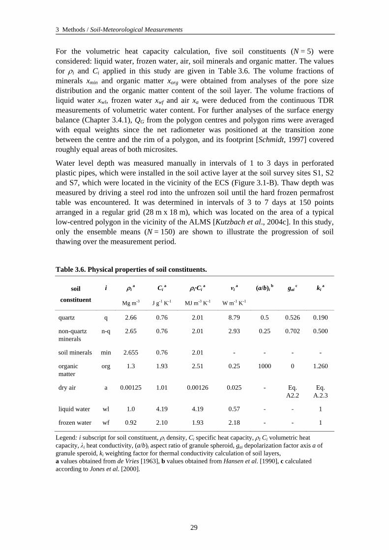
3 Methods / Soil-Meteorological Measurements
For the volumetric heat capacity calculation, five soil constituents (N = 5) were considered: liquid water, frozen water, air, soil minerals and organic matter. The values for ρi and Ci applied in this study are given in Table 3.6. The volume fractions of minerals xmin and organic matter xorg were obtained from analyses of the pore size distribution and the organic matter content of the soil layer. The volume fractions of liquid water xwl, frozen water xwf and air xa were deduced from the continuous TDR measurements of volumetric water content. For further analyses of the surface energy balance (Chapter 3.4.1), QG from the polygon centres and polygon rims were averaged with equal weights since the net radiometer was positioned at the transition zone between the centre and the rim of a polygon, and its footprint [Schmidt, 1997] covered roughly equal areas of both microsites.
Water level depth was measured manually in intervals of 1 to 3 days in perforated plastic pipes, which were installed in the soil active layer at the soil survey sites S1, S2 and S7, which were located in the vicinity of the ECS (Figure 3.1-B). Thaw depth was measured by driving a steel rod into the unfrozen soil until the hard frozen permafrost table was encountered. It was determined in intervals of 3 to 7 days at 150 points arranged in a regular grid (28 m x 18 m), which was located on the area of a typical low-centred polygon in the vicinity of the ALMS [Kutzbach et al., 2004c]. In this study, only the ensemble means (N = 150) are shown to illustrate the progression of soil thawing over the measurement period.
Table 3.6. Physical properties of soil constituents.
soil
constituent
i ρi a
Mg m-3
Ci a
J g-1 K-1
ρi·Ci a
MJ m-3 K-1
νi a
W m-1 K-1
(a/b)i b gai
c ki a
quartz q 2.66 0.76 2.01 8.79 0.5 0.526 0.190
non-quartz minerals
n-q 2.65 0.76 2.01 2.93 0.25 0.702 0.500
soil minerals min 2.655 0.76 2.01 - - - -
organic matter
org 1.3 1.93 2.51 0.25 1000 0 1.260
dry air a 0.00125 1.01 0.00126 0.025 - Eq. A2.2
Eq. A.2.3
liquid water wl 1.0 4.19 4.19 0.57 - - 1
frozen water wf 0.92 2.10 1.93 2.18 - - 1
Legend: i subscript for soil constituent, ρi density, Ci specific heat capacity, ρI Ci volumetric heat capacity, λi heat conductivity, (a/b)i aspect ratio of granule spheroid, gai depolarization factor axis a of granule speroid, ki weighting factor for thermal conductivity calculation of soil layers, a values obtained from de Vries [1963], b values obtained from Hansen et al. [1990], c calculated according to Jones et al. [2000].
29
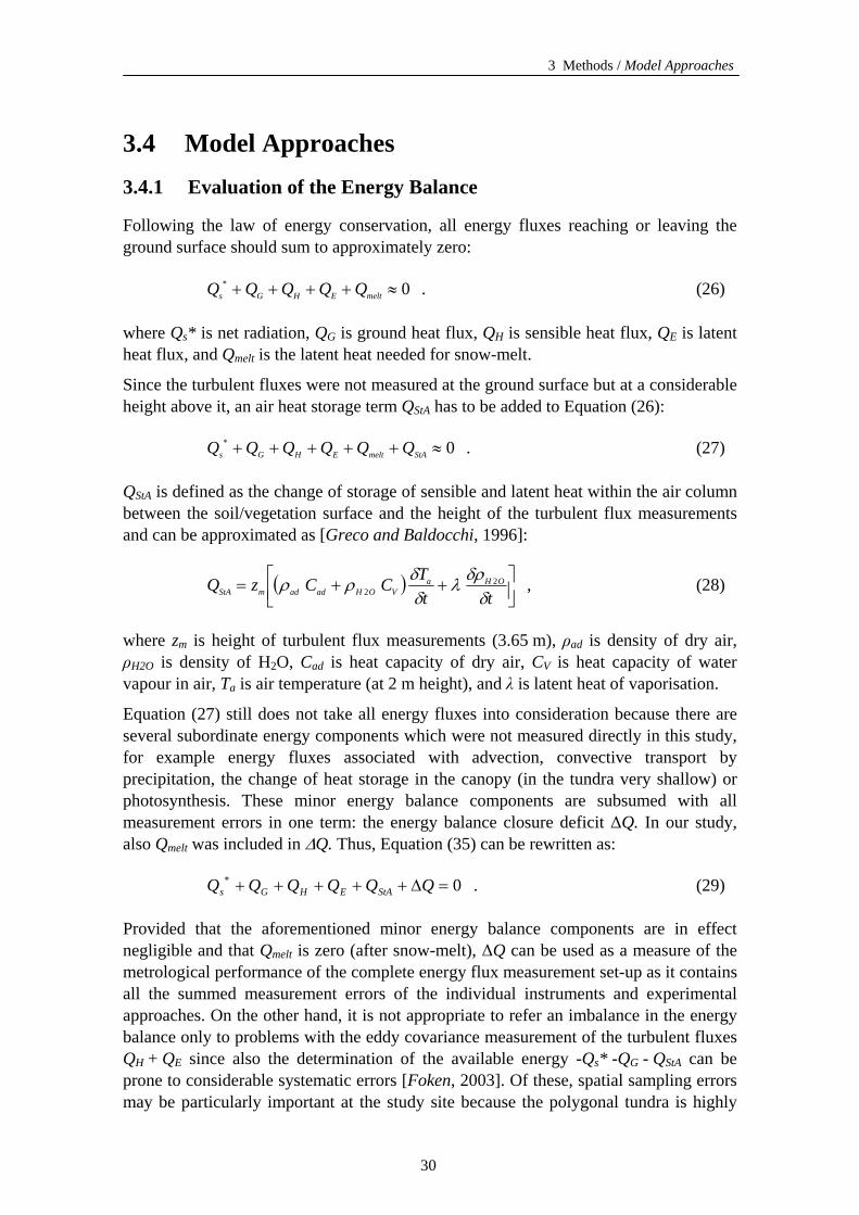
3 Methods / Model Approaches
3.4 Model Approaches 3.4.1 Evaluation of the Energy Balance
Following the law of energy conservation, all energy fluxes reaching or leaving the ground surface should sum to approximately zero:
0≈++++∗
meltEHGs QQQQQ . (26)
where Qs* is net radiation, QG is ground heat flux, QH is sensible heat flux, QE is latent heat flux, and Qmelt is the latent heat needed for snow-melt.
Since the turbulent fluxes were not measured at the ground surface but at a considerable height above it, an air heat storage term QStA has to be added to Equation (26):
0≈+++++∗
StAmeltEHGs QQQQQQ . (27)
QStA is defined as the change of storage of sensible and latent heat within the air column between the soil/vegetation surface and the height of the turbulent flux measurements and can be approximated as [Greco and Baldocchi, 1996]:
( ) ⎥⎦⎤
⎢⎣⎡ ++=
ttTCCzQ OHa
VOHadadmStA δδρλ
δδρρ 2
2 , (28)
where zm is height of turbulent flux measurements (3.65 m), ρad is density of dry air, ρH2O is density of H2O, Cad is heat capacity of dry air, CV is heat capacity of water vapour in air, Ta is air temperature (at 2 m height), and λ is latent heat of vaporisation.
Equation (27) still does not take all energy fluxes into consideration because there are several subordinate energy components which were not measured directly in this study, for example energy fluxes associated with advection, convective transport by precipitation, the change of heat storage in the canopy (in the tundra very shallow) or photosynthesis. These minor energy balance components are subsumed with all measurement errors in one term: the energy balance closure deficit ΔQ. In our study, also Qmelt was included in ΔQ. Thus, Equation (35) can be rewritten as:
0=Δ+++++∗ QQQQQQ StAEHGs . (29)
Provided that the aforementioned minor energy balance components are in effect negligible and that Qmelt is zero (after snow-melt), ΔQ can be used as a measure of the metrological performance of the complete energy flux measurement set-up as it contains all the summed measurement errors of the individual instruments and experimental approaches. On the other hand, it is not appropriate to refer an imbalance in the energy balance only to problems with the eddy covariance measurement of the turbulent fluxes QH + QE since also the determination of the available energy -Qs* -QG - QStA can be prone to considerable systematic errors [Foken, 2003]. Of these, spatial sampling errors may be particularly important at the study site because the polygonal tundra is highly
30
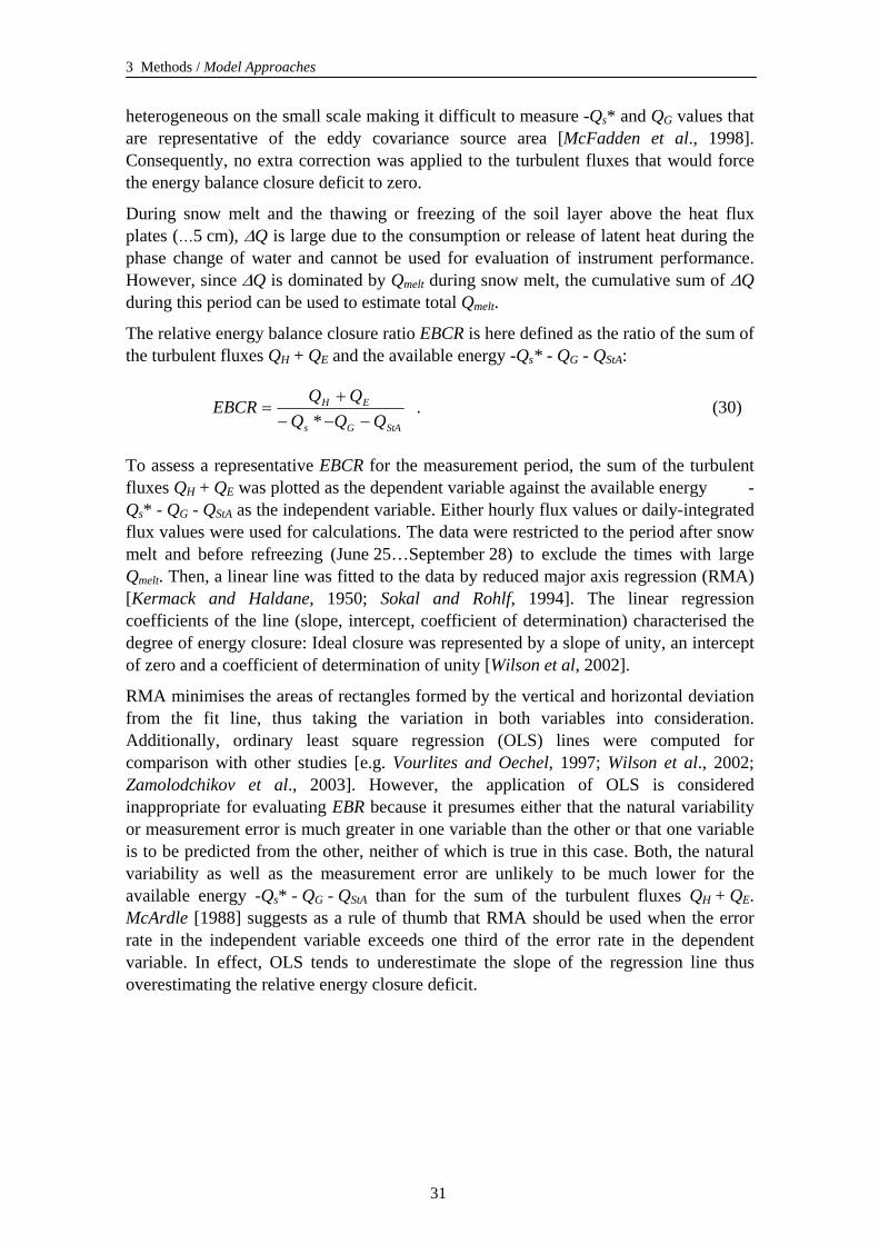
3 Methods / Model Approaches
heterogeneous on the small scale making it difficult to measure -Qs* and QG values that are representative of the eddy covariance source area [McFadden et al., 1998]. Consequently, no extra correction was applied to the turbulent fluxes that would force the energy balance closure deficit to zero.
During snow melt and the thawing or freezing of the soil layer above the heat flux
defined as the ratio of the sum of
plates (…5 cm), ΔQ is large due to the consumption or release of latent heat during the phase change of water and cannot be used for evaluation of instrument performance. However, since ΔQ is dominated by Qmelt during snow melt, the cumulative sum of ΔQ during this period can be used to estimate total Qmelt.
The relative energy balance closure ratio EBCR is herethe turbulent fluxes QH + QE and the available energy -Qs* - QG - QStA:
StAGs
EH
QQQQQ
EBCR−−−
+=
* . (30)
To assess a representative EBCR for the measurement period, the sum of the turbulent
ontal deviation
fluxes QH + QE was plotted as the dependent variable against the available energy -Qs* - QG - QStA as the independent variable. Either hourly flux values or daily-integrated flux values were used for calculations. The data were restricted to the period after snow melt and before refreezing (June 25…September 28) to exclude the times with large Qmelt. Then, a linear line was fitted to the data by reduced major axis regression (RMA) [Kermack and Haldane, 1950; Sokal and Rohlf, 1994]. The linear regression coefficients of the line (slope, intercept, coefficient of determination) characterised the degree of energy closure: Ideal closure was represented by a slope of unity, an intercept of zero and a coefficient of determination of unity [Wilson et al, 2002].
RMA minimises the areas of rectangles formed by the vertical and horizfrom the fit line, thus taking the variation in both variables into consideration. Additionally, ordinary least square regression (OLS) lines were computed for comparison with other studies [e.g. Vourlites and Oechel, 1997; Wilson et al., 2002; Zamolodchikov et al., 2003]. However, the application of OLS is considered inappropriate for evaluating EBR because it presumes either that the natural variability or measurement error is much greater in one variable than the other or that one variable is to be predicted from the other, neither of which is true in this case. Both, the natural variability as well as the measurement error are unlikely to be much lower for the available energy -Qs* - QG - QStA than for the sum of the turbulent fluxes QH + QE. McArdle [1988] suggests as a rule of thumb that RMA should be used when the error rate in the independent variable exceeds one third of the error rate in the dependent variable. In effect, OLS tends to underestimate the slope of the regression line thus overestimating the relative energy closure deficit.
31
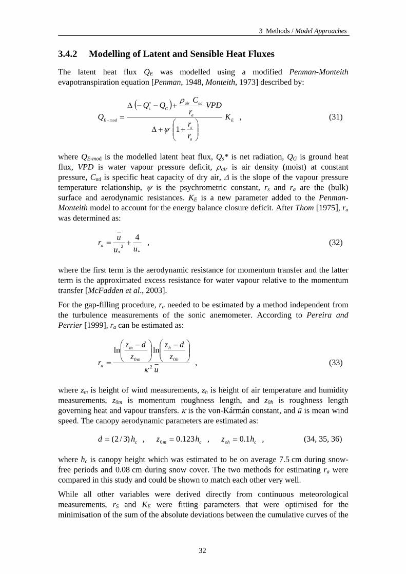
3 Methods / Model Approaches
3.4.2 Modelling of Latent and Sensible Heat Fluxes
E Penman-Monteith The latent heat flux Q was modelled using a modified evapotranspiration equation [Penman, 1948, Monteith, 1973] described by:
( )E
a
s
a
adairGs
E K
rr
VPDrCQQ
Q
⎟⎟⎠
⎞⎜⎜⎝
⎛++Δ
+−−Δ=
∗
−
1mod
ψ
ρ
, (31)
where QE-mod is the modelled latent heat flux, Qs* is net radiation, QG is ground heat flux, VPD is water vapour pressure deficit, ρair is air density (moist) at constant pressure, Cad is specific heat capacity of dry air, Δ is the slope of the vapour pressure temperature relationship, ψ is the psychrometric constant, rs and ra are the (bulk) surface and aerodynamic resistances. KE is a new parameter added to the Penman-Monteith model to account for the energy balance closure deficit. After Thom [1975], ra was determined as:
*2
*
4uu
ura += , (32)
where the first term is the aerodynamic resistance for momentum transfer and the latter
eeded to be estimated by a method independent from
term is the approximated excess resistance for water vapour relative to the momentum transfer [McFadden et al., 2003].
For the gap-filling procedure, ra nthe turbulence measurements of the sonic anemometer. According to Pereira and Perrier [1999], ra can be estimated as:
uz
dzz
dz
r h
h
m
m
a 200
lnln
κ
⎟⎟⎠
⎞⎜⎜⎝
⎛ −⎟⎟⎠
⎞⎜⎜⎝
⎛ −
= , (33)
where zm is height of wind measurements, zh is height of air temperature and humidity measurements, z0m is momentum roughness length, and z0h is roughness length governing heat and vapour transfers. κ is the von-Kármán constant, and ū is mean wind speed. The canopy aerodynamic parameters are estimated as:
, chd )3/2(= cm hz 123.00 = coh hz 1.0= , , (34, 35, 36)
where hc is canopy height which was estimated to be on average 7.5 cm during snow-
eteorological
free periods and 0.08 cm during snow cover. The two methods for estimating ra were compared in this study and could be shown to match each other very well.
While all other variables were derived directly from continuous mmeasurements, rS and KE were fitting parameters that were optimised for the minimisation of the sum of the absolute deviations between the cumulative curves of the
32
3 Methods / Model Approaches
modelled latent heat fluxes QE-mod-cumul and the measured latent heat fluxes QE-meas-cumul, respectively (Figure 3.4). For both campaigns 2003 and 2004, rs was 44.49 s m-1 and KE was 0.785.
The sensible heat flux QH was modelled by an energy closure approach:
( ) HEGsH KQQQQ −−−=− *mod , (37)
where QH-mod is the modelled sensible heat flux, and KH is a fitting parameter that
y inversion of the Penman-
accounts for the energy closure deficit. KH is optimised for the minimisation of the sum of the absolute deviations between the cumulative curve of the modelled sensible heat fluxes QH-mod-cumul and the cumulative curve of the measured sensible heat fluxes QH-meas-cumul (Figure 3.4). KH was 0.88 in 2003 and 0.95 in 2004. The scatter plots in Figure 3.5 reveal a considerable inaccuracy of the heat flux models (QE: R = 0.95; QH: R = 0.96). Both, substantial underestimates and overestimates are common. However, these negative and positive errors tend to cancel each other over longer periods due to the applied parameter optimisation method.
With QE measured by the ECS, rs could be determined bMonteith equation. To quantify the coupling between the tundra vegetation and the atmospheric boundary layer, the decoupling coefficient Ω [Jarvis and Naughton, 1986] was calculated as:
( )as rr++Δ+Δ
=Ω1ψ
ψ . (38)
Midday averages of rs and Ω were calculated by averaging the hourly intervals with
rs is the surface-to-air water vapour pressure deficit
S↓ > 130 W m-2 which was encountered from 3:00 to 21:00 on clear days around the summer solstice and from 9:00 to 15:00 at the end of September. This filter excluded also very cloudy, rainy days.
An important control on ET and VPDs-a [Vourlites and Oechel, 1999], which is calculated as:
( )mmmsas eTeVPD 6.300 −= −− , (39)
where es-0m is the saturation water vapour pressure at the surface, which is a function of the large-scale surface temperature T0m., which is determined by inversion of the sensible heat flux equation:
adair
aHmm C
rQTT
ρ6.30 = . (40)
33
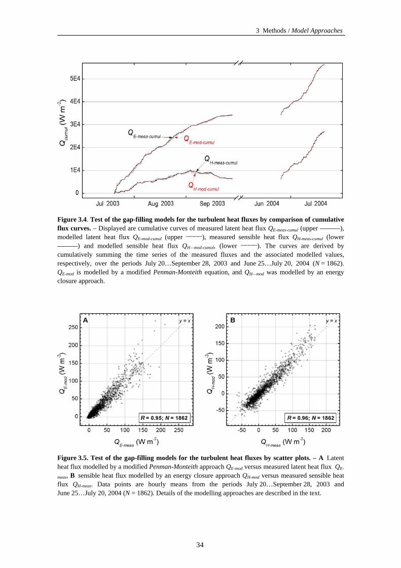
3 Methods / Model Approaches
Figure 3.4. Test of the gap-filling models for the turbulent heat fluxes by comparison of cumulative flux curves. – Displayed are cumulative curves of measured latent heat flux QE-meas-cumul (upper ———), modelled latent heat flux QE-mod-cumul (upper ┈┈┈┈), measured sensible heat flux QH-meas-cumul (lower ———) and modelled sensible heat flux QH—mod-cumul, (lower ┈┈┈┈). The curves are derived by cumulatively summing the time series of the measured fluxes and the associated modelled values, respectively, over the periods July 20…September 28, 2003 and June 25…July 20, 2004 (N = 1862). QE-mod is modelled by a modified Penman-Monteith equation, and QH—mod was modelled by an energy closure approach.
Figure 3.5. Test of the gap-filling models for the turbulent heat fluxes by scatter plots. – A Latent heat flux modelled by a modified Penman-Monteith approach QE-mod versus measured latent heat flux QE-
meas, B sensible heat flux modelled by an energy closure approach QH-mod versus measured sensible heat flux QH-meas. Data points are hourly means from the periods July 20…September 28, 2003 and June 25…July 20, 2004 (N = 1862). Details of the modelling approaches are described in the text.
34
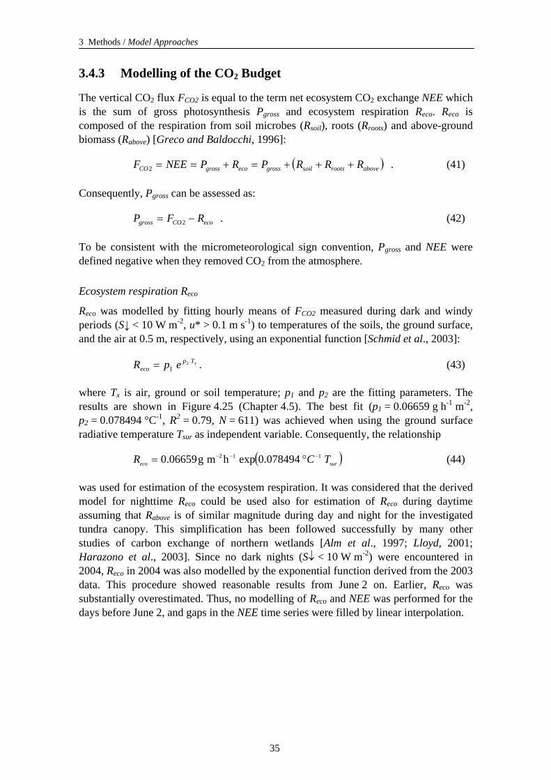
3 Methods / Model Approaches
3.4.3 Modelling of the CO2 Budget
The vertical CO2 flux FCO2 is equal to the term net ecosystem CO2 exchange NEE which is the sum of gross photosynthesis Pgross and ecosystem respiration Reco. Reco is composed of the respiration from soil microbes (Rsoil), roots (Rroots) and above-ground biomass (Rabove) [Greco and Baldocchi, 1996]:
( )aboverootssoilgrossecogrossCO RRRPRPNEEF +++=+==2 . (41)
Consequently, Pgross can be assessed as:
ecoCOgross RFP −= 2 . (42)
To be consistent with the micrometeorological sign convention, Pgross and NEE were defined negative when they removed CO2 from the atmosphere.
Ecosystem respiration Reco
Reco was modelled by fitting hourly means of FCO2 measured during dark and windy periods (S↓ < 10 W m-2, u* > 0.1 m s-1) to temperatures of the soils, the ground surface, and the air at 0.5 m, respectively, using an exponential function [Schmid et al., 2003]:
xTpeco epR 2
1= . (43)
where Tx is air, ground or soil temperature; p1 and p2 are the fitting parameters. The results are shown in Figure 4.25 (Chapter 4.5). The best fit (p1 = 0.06659 g h-1 m-2, p2 = 0.078494 °C-1, R2 = 0.79, N = 611) was achieved when using the ground surface radiative temperature Tsur as independent variable. Consequently, the relationship
( )sureco TCR 112 078494.0exphmg06659.0 −−− °= (44)
was used for estimation of the ecosystem respiration. It was considered that the derived model for nighttime Reco could be used also for estimation of Reco during daytime assuming that Rabove is of similar magnitude during day and night for the investigated tundra canopy. This simplification has been followed successfully by many other studies of carbon exchange of northern wetlands [Alm et al., 1997; Lloyd, 2001; Harazono et al., 2003]. Since no dark nights (S↓ < 10 W m-2) were encountered in 2004, Reco in 2004 was also modelled by the exponential function derived from the 2003 data. This procedure showed reasonable results from June 2 on. Earlier, Reco was substantially overestimated. Thus, no modelling of Reco and NEE was performed for the days before June 2, and gaps in the NEE time series were filled by linear interpolation.
35
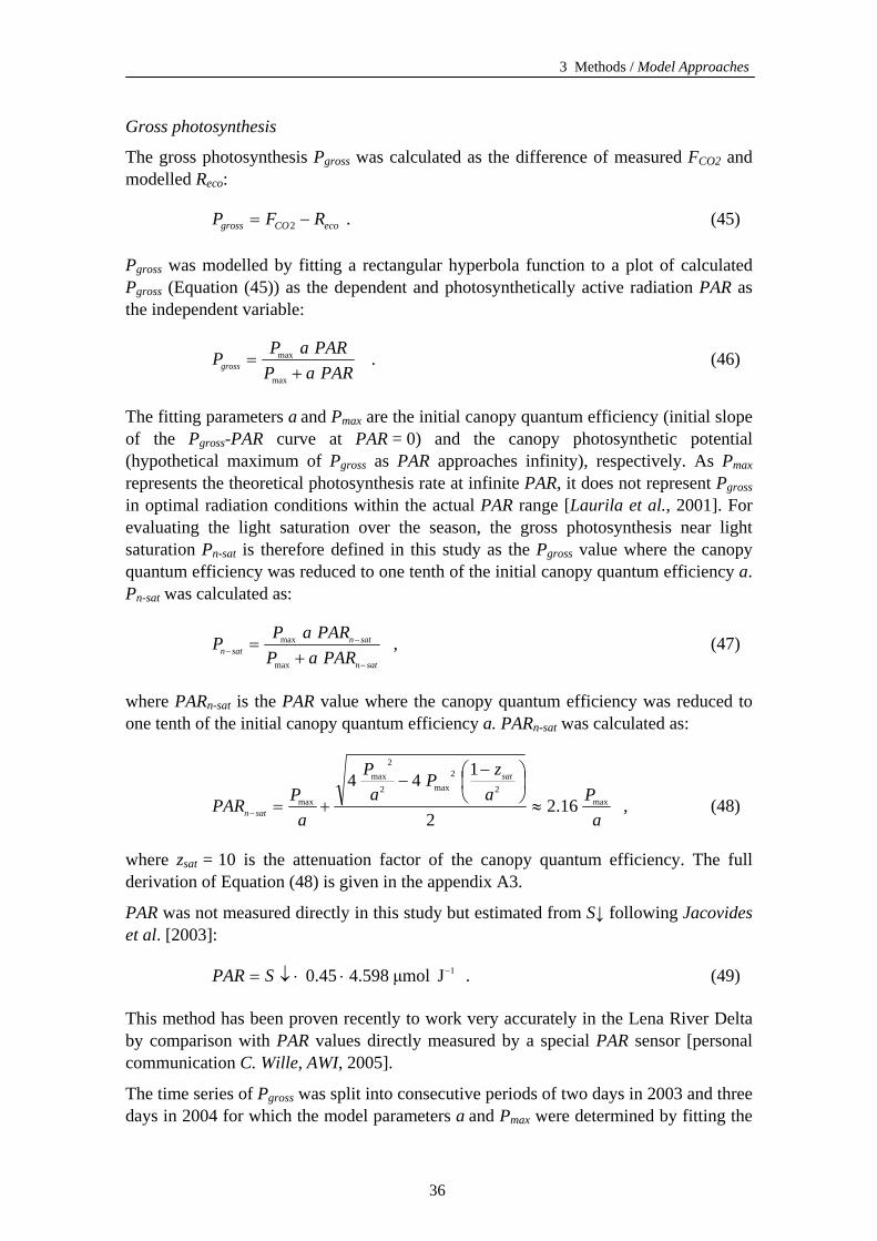
3 Methods / Model Approaches
Gross photosynthesis
The gross photosynthesis Pgross was calculated as the difference of measured FCO2 and modelled Reco:
ecoCOgross RFP −= 2 . (45)
Pgross was modelled by fitting a rectangular hyperbola function to a plot of calculated Pgross (Equation (45)) as the dependent and photosynthetically active radiation PAR as the independent variable:
PARaPPARaPPgross +
=max
max . (46)
The fitting parameters a and Pmax are the initial canopy quantum efficiency (initial slope of the Pgross-PAR curve at PAR = 0) and the canopy photosynthetic potential (hypothetical maximum of Pgross as PAR approaches infinity), respectively. As Pmax represents the theoretical photosynthesis rate at infinite PAR, it does not represent Pgross in optimal radiation conditions within the actual PAR range [Laurila et al., 2001]. For evaluating the light saturation over the season, the gross photosynthesis near light saturation Pn-sat is therefore defined in this study as the Pgross value where the canopy quantum efficiency was reduced to one tenth of the initial canopy quantum efficiency a. Pn-sat was calculated as:
satn
satnsatn PARaP
PARaPP−
−− +
=max
max , (47)
where PARn-sat is the PAR value where the canopy quantum efficiency was reduced to one tenth of the initial canopy quantum efficiency a. PARn-sat was calculated as:
aPa
zPa
P
aPPAR
sat
satnmax
2
2max2
2max
max 16.22
144≈
⎟⎠⎞
⎜⎝⎛ −
−+=− , (48)
where zsat = 10 is the attenuation factor of the canopy quantum efficiency. The full derivation of Equation (48) is given in the appendix A3.
PAR was not measured directly in this study but estimated from S↓ following Jacovides et al. [2003]:
1Jμmol598.445.0 −⋅⋅↓= SPAR . (49)
This method has been proven recently to work very accurately in the Lena River Delta by comparison with PAR values directly measured by a special PAR sensor [personal communication C. Wille, AWI, 2005].
The time series of Pgross was split into consecutive periods of two days in 2003 and three days in 2004 for which the model parameters a and Pmax were determined by fitting the
36
3 Methods / Model Approaches
theoretical curve to the data. A relatively short period of two to three days was chosen to reflect the rapid changes of the tundra vegetation, temperature and cloudiness conditions which influence the light response curve. Modelling of one-day periods for 2003 or two-day periods for 2004 did not work reliably due to the often insufficient number of data points. Examples of the Pgross modelling are given for August 1…2, 2003 and September 2…3, 2003 in Figure 3.6.
Figure 3.6. Examples for the relationship between gross photosynthesis Pgross and photosynthetically active radiation PAR. – A August 1…2, 2003, B September 2…3, 2003. Data points are hourly means of calculated Pgross (= FCO2 - Reco). Rectangular hyperbola functions were fitted to the data with the fitting parameters Pmax and a, which are the canopy photosynthetic potential and the initial canopy quantum efficiency, respectively. The white stars indicate the point where the canopy quantum efficiency (the slope of the light response curve) was reduced to one tenth of its initial value a and Pn-sat is reached.
37
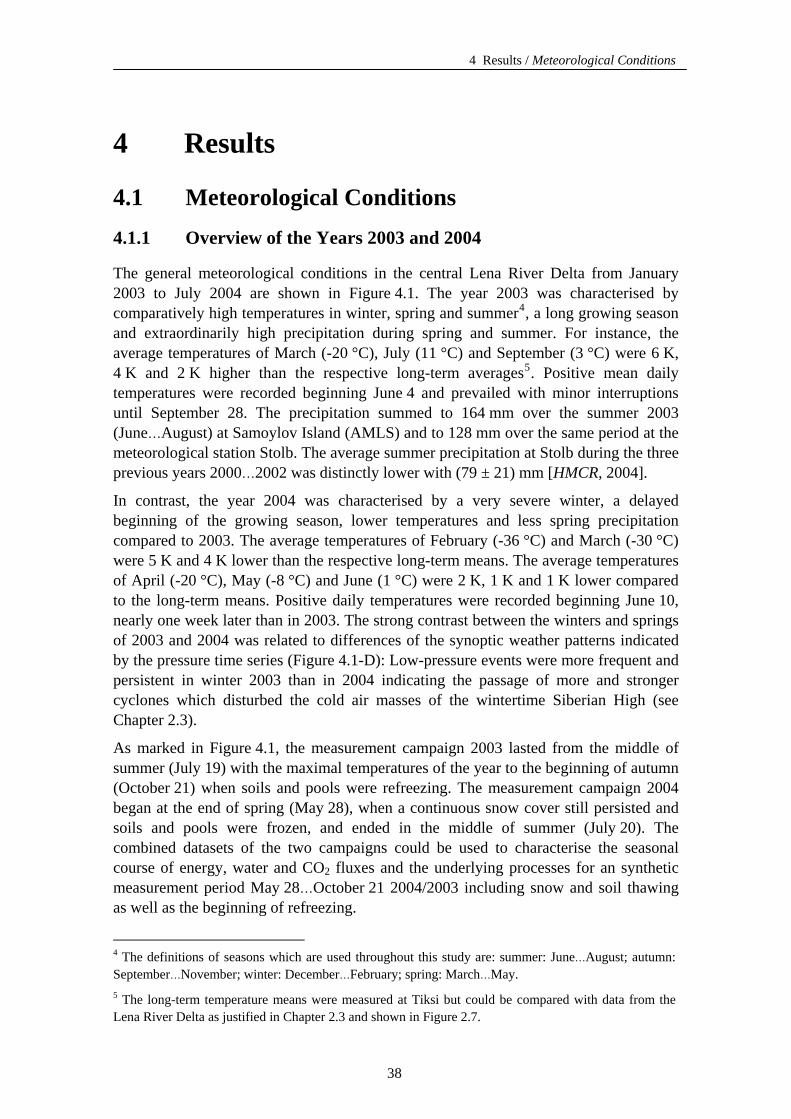
4 Results / Meteorological Conditions
4 Results
4.1 Meteorological Conditions 4.1.1 Overview of the Years 2003 and 2004
The general meteorological conditions in the central Lena River Delta from January 2003 to July 2004 are shown in Figure 4.1. The year 2003 was characterised by comparatively high temperatures in winter, spring and summer4, a long growing season and extraordinarily high precipitation during spring and summer. For instance, the average temperatures of March (-20 °C), July (11 °C) and September (3 °C) were 6 K, 4 K and 2 K higher than the respective long-term averages5. Positive mean daily temperatures were recorded beginning June 4 and prevailed with minor interruptions until September 28. The precipitation summed to 164 mm over the summer 2003 (June…August) at Samoylov Island (AMLS) and to 128 mm over the same period at the meteorological station Stolb. The average summer precipitation at Stolb during the three previous years 2000…2002 was distinctly lower with (79 ± 21) mm [HMCR, 2004].
In contrast, the year 2004 was characterised by a very severe winter, a delayed beginning of the growing season, lower temperatures and less spring precipitation compared to 2003. The average temperatures of February (-36 °C) and March (-30 °C) were 5 K and 4 K lower than the respective long-term means. The average temperatures of April (-20 °C), May (-8 °C) and June (1 °C) were 2 K, 1 K and 1 K lower compared to the long-term means. Positive daily temperatures were recorded beginning June 10, nearly one week later than in 2003. The strong contrast between the winters and springs of 2003 and 2004 was related to differences of the synoptic weather patterns indicated by the pressure time series (Figure 4.1-D): Low-pressure events were more frequent and persistent in winter 2003 than in 2004 indicating the passage of more and stronger cyclones which disturbed the cold air masses of the wintertime Siberian High (see Chapter 2.3).
As marked in Figure 4.1, the measurement campaign 2003 lasted from the middle of summer (July 19) with the maximal temperatures of the year to the beginning of autumn (October 21) when soils and pools were refreezing. The measurement campaign 2004 began at the end of spring (May 28), when a continuous snow cover still persisted and soils and pools were frozen, and ended in the middle of summer (July 20). The combined datasets of the two campaigns could be used to characterise the seasonal course of energy, water and CO2 fluxes and the underlying processes for an synthetic measurement period May 28…October 21 2004/2003 including snow and soil thawing as well as the beginning of refreezing.
4 The definitions of seasons which are used throughout this study are: summer: June…August; autumn: September…November; winter: December…February; spring: March…May. 5 The long-term temperature means were measured at Tiksi but could be compared with data from the Lena River Delta as justified in Chapter 2.3 and shown in Figure 2.7.
38
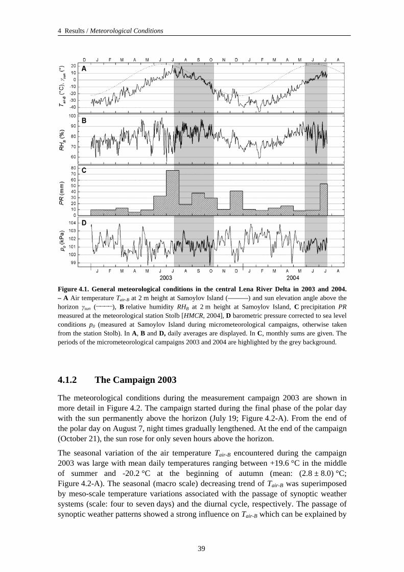
4 Results / Meteorological Conditions
Figure 4.1. General meteorological conditions in the central Lena River Delta in 2003 and 2004. – A Air temperature Tair-B at 2 m height at Samoylov Island (———) and sun elevation angle above the horizon γsun (┈┈┈┈), B relative humidity RHB at 2 m height at Samoylov Island, C precipitation PR measured at the meteorological station Stolb [HMCR, 2004], D barometric pressure corrected to sea level conditions p0 (measured at Samoylov Island during micrometeorological campaigns, otherwise taken from the station Stolb). In A, B and D, daily averages are displayed. In C, monthly sums are given. The periods of the micrometeorological campaigns 2003 and 2004 are highlighted by the grey background.
4.1.2 The Campaign 2003
The meteorological conditions during the measurement campaign 2003 are shown in more detail in Figure 4.2. The campaign started during the final phase of the polar day with the sun permanently above the horizon (July 19; Figure 4.2-A). From the end of the polar day on August 7, night times gradually lengthened. At the end of the campaign (October 21), the sun rose for only seven hours above the horizon.
The seasonal variation of the air temperature Tair-B encountered during the campaign 2003 was large with mean daily temperatures ranging between +19.6 °C in the middle of summer and -20.2 °C at the beginning of autumn (mean: (2.8 ± 8.0) °C; Figure 4.2-A). The seasonal (macro scale) decreasing trend of T
B
air-BB was superimposed by meso-scale temperature variations associated with the passage of synoptic weather systems (scale: four to seven days) and the diurnal cycle, respectively. The passage of synoptic weather patterns showed a strong influence on Tair-B which can be explained by B
39
4 Results / Meteorological Conditions
the situation of the Lena River Delta at the interface between the Arctic Ocean and the Eurasian continent. Periods of comparatively high Tair-BB were regularly linked with southerly winds from the Siberian mainland whereas cool periods were connected to northerly winds from the Arctic Ocean. On the other hand, the diurnal variations of Tair-B were moderate with an average daily temperature span of (5 ± 3) K as it is typical for maritime Arctic climates.
B
The relative humidity RHB ranged during the measurement campaign 2003 between 99 % and 35 % with a mean of (84 ± 9) % (Figure 4.2-B). The seasonal variation of RH
B
BB was less pronounced compared to Tair-B. Most of the variability of RHB BB was associated to the diurnal cycle with the maximum occurring between midnight and early morning (0:00…8:00) and a minimum in the afternoon between 14:00 and 18:00. The fluctuations of p0 were low for the most part (Figure 4.2-D). The mean amounted to (101.2 ± 0.7) kPa. The extreme values were 98.4 kPa and 103.2 kPa, respectively. Decreasing pressure was associated with southerly winds and rising air temperatures indicating the advection of continental air masses from the South to the investigation site.
A big part of the high total summer precipitation in 2003 as mentioned in Chapter 4.1.1 was recorded during several particularly strong rainfall events at the beginning of the measurement campaign at the end of July (94 mm in six days, Figure 4.2-C). During August, the precipitation was below and during September again considerably above the averages for the preceding years 2000…2002 [HMCR, 2004]. The precipitation pattern was reflected by the water table levels measured at the centre and the rim of a polygon near to the micrometeorological tower (Figure 4.2-E): Maximum water table heights were observed with 8 cm above soil surface in the polygon centre and 8 cm below the soil surface at the polygon rim on July 25, when the strongest rainfall event occurred. Afterwards, the water table heights decreased gradually and reached their minimum at the end of September with 0 cm above soil surface in the centre and 13 cm below the soil surface at the rim. Before freezing of the soils (July 19…September 28), the volumetric water content in the top soil θS-5cm amounted to (97 ± 1) % (saturation: 98 %) and (30 ± 1) % (saturation: 47 %) in the centre and at the rim of the polygon, respectively (Figure 4.2-G). After freezing of the top soil layer (October 8…21), the liquid water content was reduced to (6 ± 1) % and (11 ± 1) % in the centre and at the rim, respectively. These rather high values indicate inadequate calibration of the TDR probes at low liquid water content.
The thaw depth increased during the measurement campaign 2003 from (28 ± 7) cm at the beginning of the campaign (July 15) to a maximum of (48 ± 6) cm on September 12 (Figure 4.2-E). Afterwards it decreased slowly again due to refreezing from the bottom. Freezing of the soils from the top began not until September 29 due to the relatively high temperatures in September. At the end of the campaign on October 21, the soils were on average frozen down to a depth of approximately 30 cm. At that time, unfrozen soil zones of several decimetres still persisted below the frozen top soil layer. A closed snow cover built up beginning October 9. At the end of the campaign, the snow cover reached a thickness of about 10 cm in the polygon centres (Figure 4.2-E) and about 1…2 cm at the rims (measured manually, data not shown). The albedo α of the surface averaged during summer 0.15 ± 0.05 (July 19…September 28), when the soil was
40
4 Results / Meteorological Conditions
Figure 4.2. Meteorological and soil conditions on Samoylov Island during the campaign 2003. – A Tair-B at 2 m height (——) and γsun (┈┈┈┈), B RHB at 2 m height, C daily sums of PR, D p0, E heights h above soil surface of water table at centre (—□—) and rim (—■—) of polygon, frozen ground table (——, spatial mean: N = 150) and snow height (┈┈┈┈), F daily average albedo α (sunlight), G soil volumetric water content at 5 cm depth ΘS-5cm at centre (——) and rim (┈┈┈┈) of polygon, H soil temperatures TS at the polygon centre at depths of 1 cm (—◇—), 10 cm (—■—), 20 cm (—○—), 30 cm (—▼—) and 40 cm (—△—). In A, B, D, G and H hourly means are displayed.
41
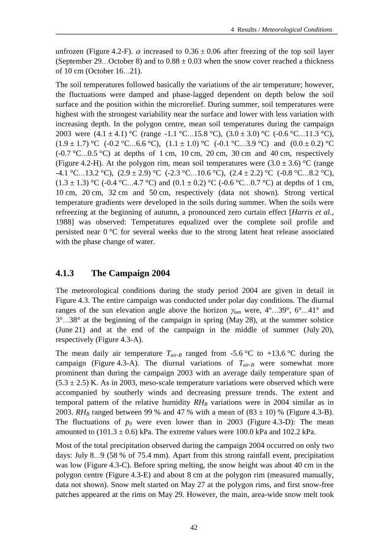
4 Results / Meteorological Conditions
unfrozen (Figure 4.2-F). α increased to 0.36 ± 0.06 after freezing of the top soil layer (September 29…October 8) and to 0.88 ± 0.03 when the snow cover reached a thickness of 10 cm (October 16…21).
The soil temperatures followed basically the variations of the air temperature; however, the fluctuations were damped and phase-lagged dependent on depth below the soil surface and the position within the microrelief. During summer, soil temperatures were highest with the strongest variability near the surface and lower with less variation with increasing depth. In the polygon centre, mean soil temperatures during the campaign 2003 were (4.1 ± 4.1) °C (range -1.1 °C…15.8 °C), (3.0 ± 3.0) °C (-0.6 °C…11.3 °C), (1.9 ± 1.7) °C (-0.2 °C…6.6 °C), (1.1 ± 1.0) °C (-0.1 °C…3.9 °C) and (0.0 ± 0.2) °C (-0.7 °C…0.5 °C) at depths of 1 cm, 10 cm, 20 cm, 30 cm and 40 cm, respectively (Figure 4.2-H). At the polygon rim, mean soil temperatures were (3.0 ± 3.6) °C (range -4.1 °C…13.2 °C), (2.9 ± 2.9) °C (-2.3 °C…10.6 °C), (2.4 ± 2.2) °C (-0.8 °C…8.2 °C), (1.3 ± 1.3) °C (-0.4 °C…4.7 °C) and (0.1 ± 0.2) °C (-0.6 °C…0.7 °C) at depths of 1 cm, 10 cm, 20 cm, 32 cm and 50 cm, respectively (data not shown). Strong vertical temperature gradients were developed in the soils during summer. When the soils were refreezing at the beginning of autumn, a pronounced zero curtain effect [Harris et al., 1988] was observed: Temperatures equalized over the complete soil profile and persisted near 0 °C for several weeks due to the strong latent heat release associated with the phase change of water.
4.1.3 The Campaign 2004
The meteorological conditions during the study period 2004 are given in detail in Figure 4.3. The entire campaign was conducted under polar day conditions. The diurnal ranges of the sun elevation angle above the horizon γsun were, 4°…39°, 6°…41° and 3°…38° at the beginning of the campaign in spring (May 28), at the summer solstice (June 21) and at the end of the campaign in the middle of summer (July 20), respectively (Figure 4.3-A).
The mean daily air temperature Tair-B ranged from -5.6 °C to +13.6 °C during the campaign (Figure 4.3-A). The diurnal variations of T
B
air-BB were somewhat more prominent than during the campaign 2003 with an average daily temperature span of (5.3 ± 2.5) K. As in 2003, meso-scale temperature variations were observed which were accompanied by southerly winds and decreasing pressure trends. The extent and temporal pattern of the relative humidity RHB variations were in 2004 similar as in 2003. RH
B
BB ranged between 99 % and 47 % with a mean of (83 ± 10) % (Figure 4.3-B). The fluctuations of p0 were even lower than in 2003 (Figure 4.3-D): The mean amounted to (101.3 ± 0.6) kPa. The extreme values were 100.0 kPa and 102.2 kPa.
Most of the total precipitation observed during the campaign 2004 occurred on only two days: July 8…9 (58 % of 75.4 mm). Apart from this strong rainfall event, precipitation was low (Figure 4.3-C). Before spring melting, the snow height was about 40 cm in the polygon centre (Figure 4.3-E) and about 8 cm at the polygon rim (measured manually, data not shown). Snow melt started on May 27 at the polygon rims, and first snow-free patches appeared at the rims on May 29. However, the main, area-wide snow melt took
42
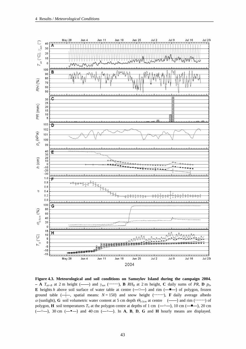
4 Results / Meteorological Conditions
Figure 4.3. Meteorological and soil conditions on Samoylov Island during the campaign 2004. – A Tair-B at 2 m height (——) and γsun (┈┈┈┈), B RHB at 2 m height, C daily sums of PR, D p0, E heights h above soil surface of water table at centre (—□—) and rim (—■—) of polygon, frozen ground table (——, spatial means: N = 150) and snow height (┈┈┈┈), F daily average albedo α (sunlight), G soil volumetric water content at 5 cm depth ΘS-5cm at centre (——) and rim (┈┈┈┈) of polygon, H soil temperatures TS at the polygon centre at depths of 1 cm (—◇—), 10 cm (—■—), 20 cm (—○—), 30 cm (—▼—) and 40 cm (—△—). In A, B, D, G and H hourly means are displayed.
43
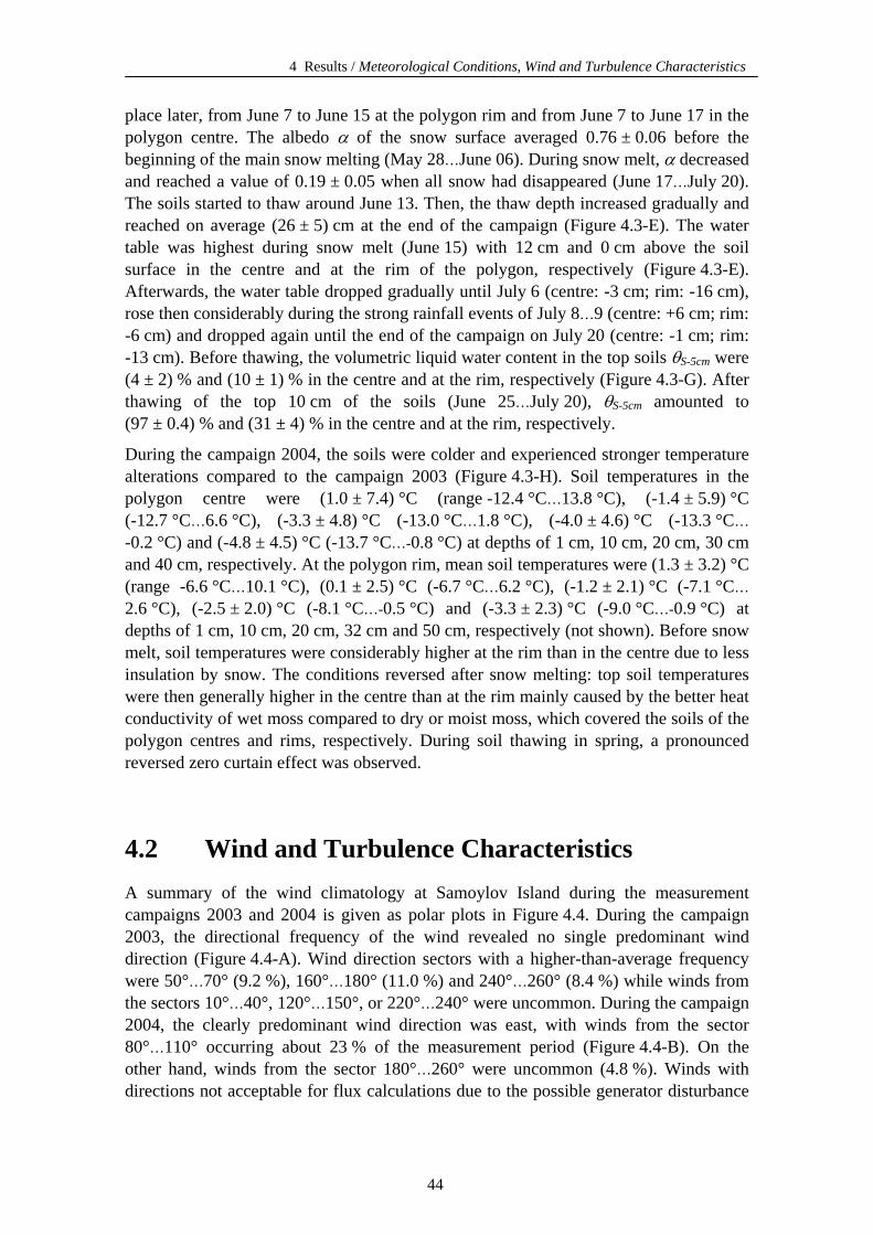
4 Results / Meteorological Conditions, Wind and Turbulence Characteristics
place later, from June 7 to June 15 at the polygon rim and from June 7 to June 17 in the polygon centre. The albedo α of the snow surface averaged 0.76 ± 0.06 before the beginning of the main snow melting (May 28…June 06). During snow melt, α decreased and reached a value of 0.19 ± 0.05 when all snow had disappeared (June 17…July 20). The soils started to thaw around June 13. Then, the thaw depth increased gradually and reached on average (26 ± 5) cm at the end of the campaign (Figure 4.3-E). The water table was highest during snow melt (June 15) with 12 cm and 0 cm above the soil surface in the centre and at the rim of the polygon, respectively (Figure 4.3-E). Afterwards, the water table dropped gradually until July 6 (centre: -3 cm; rim: -16 cm), rose then considerably during the strong rainfall events of July 8…9 (centre: +6 cm; rim: -6 cm) and dropped again until the end of the campaign on July 20 (centre: -1 cm; rim: -13 cm). Before thawing, the volumetric liquid water content in the top soils θS-5cm were (4 ± 2) % and (10 ± 1) % in the centre and at the rim, respectively (Figure 4.3-G). After thawing of the top 10 cm of the soils (June 25…July 20), θS-5cm amounted to (97 ± 0.4) % and (31 ± 4) % in the centre and at the rim, respectively.
During the campaign 2004, the soils were colder and experienced stronger temperature alterations compared to the campaign 2003 (Figure 4.3-H). Soil temperatures in the polygon centre were (1.0 ± 7.4) °C (range -12.4 °C…13.8 °C), (-1.4 ± 5.9) °C (-12.7 °C…6.6 °C), (-3.3 ± 4.8) °C (-13.0 °C…1.8 °C), (-4.0 ± 4.6) °C (-13.3 °C… -0.2 °C) and (-4.8 ± 4.5) °C (-13.7 °C…-0.8 °C) at depths of 1 cm, 10 cm, 20 cm, 30 cm and 40 cm, respectively. At the polygon rim, mean soil temperatures were (1.3 ± 3.2) °C (range -6.6 °C…10.1 °C), (0.1 ± 2.5) °C (-6.7 °C…6.2 °C), (-1.2 ± 2.1) °C (-7.1 °C… 2.6 °C), (-2.5 ± 2.0) °C (-8.1 °C…-0.5 °C) and (-3.3 ± 2.3) °C (-9.0 °C…-0.9 °C) at depths of 1 cm, 10 cm, 20 cm, 32 cm and 50 cm, respectively (not shown). Before snow melt, soil temperatures were considerably higher at the rim than in the centre due to less insulation by snow. The conditions reversed after snow melting: top soil temperatures were then generally higher in the centre than at the rim mainly caused by the better heat conductivity of wet moss compared to dry or moist moss, which covered the soils of the polygon centres and rims, respectively. During soil thawing in spring, a pronounced reversed zero curtain effect was observed.
4.2 Wind and Turbulence Characteristics A summary of the wind climatology at Samoylov Island during the measurement campaigns 2003 and 2004 is given as polar plots in Figure 4.4. During the campaign 2003, the directional frequency of the wind revealed no single predominant wind direction (Figure 4.4-A). Wind direction sectors with a higher-than-average frequency were 50°…70° (9.2 %), 160°…180° (11.0 %) and 240°…260° (8.4 %) while winds from the sectors 10°…40°, 120°…150°, or 220°…240° were uncommon. During the campaign 2004, the clearly predominant wind direction was east, with winds from the sector 80°…110° occurring about 23 % of the measurement period (Figure 4.4-B). On the other hand, winds from the sector 180°…260° were uncommon (4.8 %). Winds with directions not acceptable for flux calculations due to the possible generator disturbance
44
4 Results / Wind and Turbulence Characteristics
(230°…270°, grey) occurred 13.5 % and 5.6 % of the observation time in 2003 and 2004, respectively.
Figure 4.4. Summarized wind data from Samoylov Island during the micrometeorological campaigns 2003 and 2004. – A, B Frequency of occurrence of wind direction during the campaigns 2003 and 2004, respectively, C, D mean wind speed ū versus wind direction during the campaigns 2003 and 2004. The grey-shaded sector indicates wind directions not acceptable for flux calculations due to possible generator disturbance (230°…270°); A, C campaign 2003, B, D campaign 2004.
Time series of the wind data during the campaigns 2003 and 2004 are shown in Figure 4.5 and Figure 4.6, respectively. In 2003, wind speed ranged between 0.2 and 11.9 m s-1 with an average of (4.7 ± 2.1) m s-1 (Figure 4.5-A). Strongest winds tended to come from east-northeast and west-southwest while lightest winds came from southeast (Figure 4.4-C). Very light winds occurred seldom, with wind speeds less than 1 m s-1 observed only for 1.4 % of the time. The friction velocity u* ranged from 0.002 to 0.91 m s-1 and averaged to (0.31 ± 0.15) m s-1 (Figure 4.5-B). 30 min intervals with insufficient turbulence, i.e. with u* < 0.1 m s-1 (Chapter 3.1.4), occurred 7.7 % of the time and were excluded from flux calculations. The footprint lengths of the measurements differed greatly between periods with and without snow cover
45
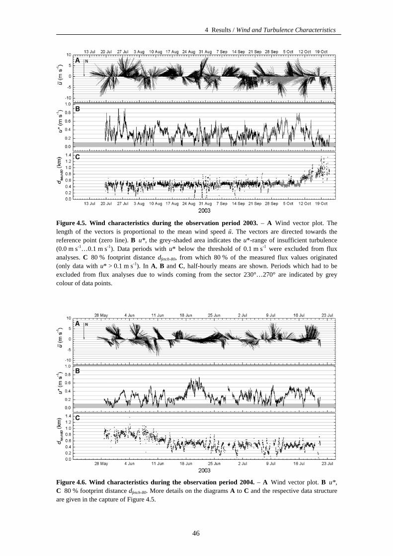
4 Results / Wind and Turbulence Characteristics
Figure 4.5. Wind characteristics during the observation period 2003. – A Wind vector plot. The length of the vectors is proportional to the mean wind speed ū. The vectors are directed towards the reference point (zero line). B u*, the grey-shaded area indicates the u*-range of insufficient turbulence (0.0 m s-1…0.1 m s-1). Data periods with u* below the threshold of 0.1 m s-1 were excluded from flux analyses. C 80 % footprint distance dfetch-80, from which 80 % of the measured flux values originated (only data with u* > 0.1 m s-1). In A, B and C, half-hourly means are shown. Periods which had to be excluded from flux analyses due to winds coming from the sector 230°…270° are indicated by grey colour of data points.
Figure 4.6. Wind characteristics during the observation period 2004. – A Wind vector plot. B u*, C 80 % footprint distance dfetch-80. More details on the diagrams A to C and the respective data structure are given in the capture of Figure 4.5.
46
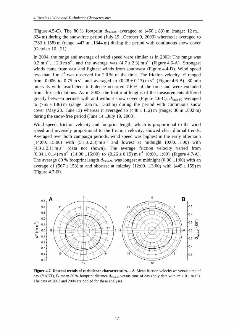
4 Results / Wind and Turbulence Characteristics
(Figure 4.5-C). The 80 % footprint dfetch-80 averaged to (460 ± 83) m (range: 12 m… 824 m) during the snow-free period (July 19…October 9, 2003) whereas it averaged to (783 ± 158) m (range: 447 m…1344 m) during the period with continuous snow cover (October 10…21).
In 2004, the range and average of wind speed were similar as in 2003: The range was 0.2 m s-1…12.3 m s-1, and the average was (4.7 ± 2.3) m s-1 (Figure 4.6-A). Strongest winds came from east and lightest winds from southwest (Figure 4.4-D). Wind speed less than 1 m s-1 was observed for 2.0 % of the time. The friction velocity u* ranged from 0.006 to 0.75 m s-1 and averaged to (0.28 ± 0.13) m s-1 (Figure 4.6-B). 30 min intervals with insufficient turbulence occurred 7.6 % of the time and were excluded from flux calculations. As in 2003, the footprint lengths of the measurements differed greatly between periods with and without snow cover (Figure 4.6-C). dfetch-80 averaged to (765 ± 136) m (range: 235 m…1363 m) during the period with continuous snow cover (May 28…June 13) whereas it averaged to (448 ± 112) m (range: 30 m…802 m) during the snow-free period (June 14…July 19, 2003).
Wind speed, friction velocity and footprint length, which is proportional to the wind speed and inversely proportional to the friction velocity, showed clear diurnal trends. Averaged over both campaign periods, wind speed was highest in the early afternoon (14:00…15:00) with (5.1 ± 2.3) m s-1 and lowest at midnight (0:00…1:00) with (4.3 ± 2.1) m s-1 (data not shown). The average friction velocity varied from (0.34 ± 0.14) m s-1 (14:00…15:00) to (0.26 ± 0.15) m s-1 (0:00…1:00) (Figure 4.7-A). The average 80 % footprint length dfetch-80 was longest at midnight (0:00…1:00) with an average of (567 ± 153) m and shortest at midday (12:00…13:00) with (449 ± 159) m (Figure 4.7-B).
Figure 4.7. Diurnal trends of turbulence characteristics. – A Mean friction velocity u* versus time of day (YAKT), B mean 80 % footprint distance dfetch-80 versus time of day (only data with u* > 0.1 m s-1). The data of 2003 and 2004 are pooled for these analyses.
47
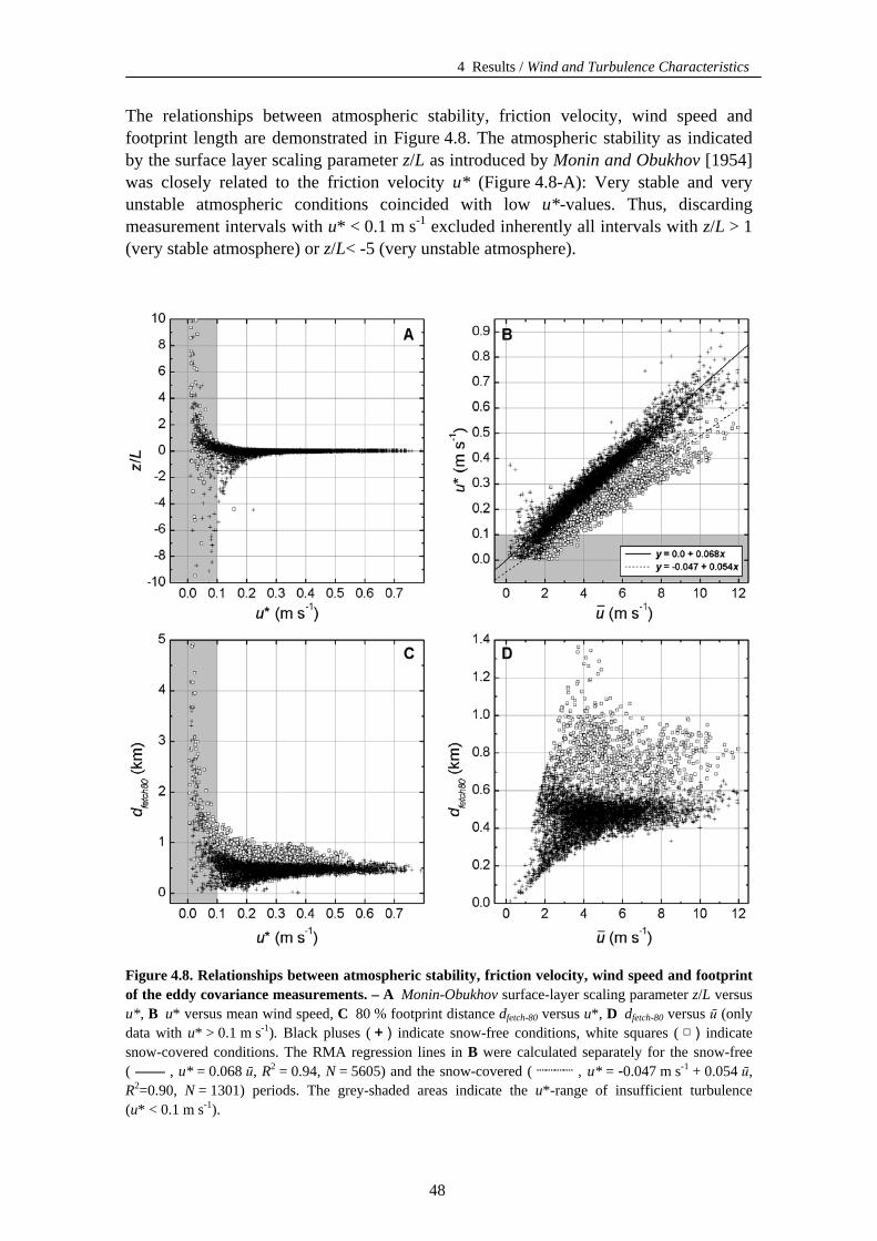
4 Results / Wind and Turbulence Characteristics
The relationships between atmospheric stability, friction velocity, wind speed and footprint length are demonstrated in Figure 4.8. The atmospheric stability as indicated by the surface layer scaling parameter z/L as introduced by Monin and Obukhov [1954] was closely related to the friction velocity u* (Figure 4.8-A): Very stable and very unstable atmospheric conditions coincided with low u*-values. Thus, discarding measurement intervals with u* < 0.1 m s-1 excluded inherently all intervals with z/L > 1 (very stable atmosphere) or z/L< -5 (very unstable atmosphere).
Figure 4.8. Relationships between atmospheric stability, friction velocity, wind speed and footprint of the eddy covariance measurements. – A Monin-Obukhov surface-layer scaling parameter z/L versus u*, B u* versus mean wind speed, C 80 % footprint distance dfetch-80 versus u*, D dfetch-80 versus ū (only data with u* > 0.1 m s-1). Black pluses ( + ) indicate snow-free conditions, white squares ( □ ) indicate snow-covered conditions. The RMA regression lines in B were calculated separately for the snow-free ( —— , u* = 0.068 ū, R2 = 0.94, N = 5605) and the snow-covered ( ┈┈┈┈ , u* = -0.047 m s-1 + 0.054 ū, R2=0.90, N = 1301) periods. The grey-shaded areas indicate the u*-range of insufficient turbulence (u* < 0.1 m s-1).
48
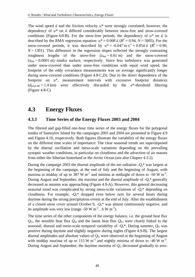
4 Results / Wind and Turbulence Characteristics, Energy Fluxes
The wind speed ū and the friction velocity u* were strongly correlated; however, the dependency of u* on ū differed considerably between snow-free and snow-covered conditions (Figure 4.8-B). For the snow-free periods, the dependency of u* on ū is described by the RMA regression equation: u* = 0.068 ū (R2 = 0.94, N = 5605). For the snow-covered periods, it was described by u* = -0.047 m s-1 + 0.054 ū (R2 = 0.90, N = 1301). This difference in the regression slopes reflected the strongly contrasting roughness lengths of the snow-free (z0m ~ 0.01 m) and the snow-covered (z0m ~ 0.0001 m) tundra surface, respectively. Since less turbulence was generated under snow-covered than under snow-free conditions with equal wind speed, the footprint of the eddy covariance measurements was on average significantly longer during snow-covered conditions (Figure 4.8-C,D). Due to the direct dependence of the footprint on u*, measurement intervals with excessive footprint distances (dfetch-80 > 1.4 km) were effectively discarded by the u*-threshold filtering (Figure 4.8-C).
4.3 Energy Fluxes 4.3.1 Time Series of the Energy Fluxes 2003 and 2004
The filtered and gap-filled one-hour time series of the energy fluxes for the polygonal tundra of Samoylov Island for the campaigns 2003 and 2004 are presented in Figure 4.9 and Figure 4.10, respectively. Both figures illustrate the variability of the energy fluxes on the different time scales of importance: The clear seasonal trends are superimposed by the diurnal oscillation and meso-scale variations depending on the prevailing synoptic weather conditions, in particular on cloudiness and the advection of air masses from either the Siberian hinterland or the Arctic Ocean (see also Chapter 4.3.2).
During the campaign 2003 the diurnal amplitude of the net radiation -Qs* was largest at the beginning of the campaign, at the end of July and the beginning of August, with maxima at midday of up to 387 W m-2 and minima at midnight of down to -50 W m-2. During August and September, the maxima and the diurnal amplitude of -Qs* generally decreased as autumn was approaching (Figure 4.9-A). However, this general decreasing seasonal trend was complicated by strong meso-scale variations of -Qs* depending on cloudiness. For example, -Qs* dropped even below zero for several hours during daytime during the strong precipitation events at the end of July. After the establishment of a closed snow cover around October 9, -Qs* was almost continuously negative, and its amplitude was very low (range -50 W m-2…6 W m-2).
The time series of the other components of the energy balance, i.e. the ground heat flux QG, the sensible heat flux QH and the latent heat flux QE, were clearly linked to the seasonal, diurnal and meso-scale temporal variability of -Qs*. During summer, QG was positive during daytime and slightly negative during nights (Figure 4.9-B). The largest diurnal amplitudes and absolute values of QG were observed at the beginning of August with midday maxima of up to 115 W m-2 and nightly minima of down to -40 W m-2. During August and September, the daytime maxima of QG decreased gradually to zero.
49
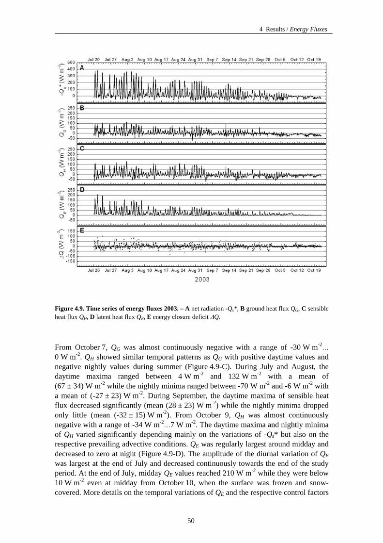
4 Results / Energy Fluxes
Figure 4.9. Time series of energy fluxes 2003. – A net radiation -Qs*, B ground heat flux QG, C sensible heat flux QH, D latent heat flux QE, E energy closure deficit ΔQ.
From October 7, QG was almost continuously negative with a range of -30 W m-2… 0 W m-2. QH showed similar temporal patterns as QG with positive daytime values and negative nightly values during summer (Figure 4.9-C). During July and August, the daytime maxima ranged between 4 W m-2 and 132 W m-2 with a mean of (67 ± 34) W m-2 while the nightly minima ranged between -70 W m-2 and -6 W m-2 with a mean of (-27 ± 23) W m-2. During September, the daytime maxima of sensible heat flux decreased significantly (mean (28 ± 23) W m-2) while the nightly minima dropped only little (mean (-32 ± 15) W m-2). From October 9, QH was almost continuously negative with a range of -34 W m-2…7 W m-2. The daytime maxima and nightly minima of QH varied significantly depending mainly on the variations of -Qs* but also on the respective prevailing advective conditions. QE was regularly largest around midday and decreased to zero at night (Figure 4.9-D). The amplitude of the diurnal variation of QE was largest at the end of July and decreased continuously towards the end of the study period. At the end of July, midday QE values reached 210 W m-2 while they were below 10 W m-2 even at midday from October 10, when the surface was frozen and snow-covered. More details on the temporal variations of QE and the respective control factors
50
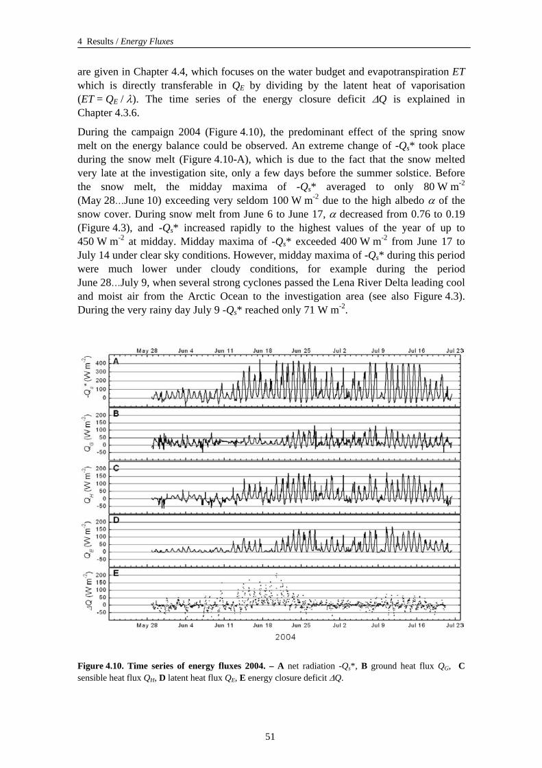
4 Results / Energy Fluxes
are given in Chapter 4.4, which focuses on the water budget and evapotranspiration ET which is directly transferable in QE by dividing by the latent heat of vaporisation (ET = QE / λ). The time series of the energy closure deficit ΔQ is explained in Chapter 4.3.6.
During the campaign 2004 (Figure 4.10), the predominant effect of the spring snow melt on the energy balance could be observed. An extreme change of -Qs* took place during the snow melt (Figure 4.10-A), which is due to the fact that the snow melted very late at the investigation site, only a few days before the summer solstice. Before the snow melt, the midday maxima of -Qs* averaged to only 80 W m-2 (May 28…June 10) exceeding very seldom 100 W m-2 due to the high albedo α of the snow cover. During snow melt from June 6 to June 17, α decreased from 0.76 to 0.19 (Figure 4.3), and -Qs* increased rapidly to the highest values of the year of up to 450 W m-2 at midday. Midday maxima of -Qs* exceeded 400 W m-2 from June 17 to July 14 under clear sky conditions. However, midday maxima of -Qs* during this period were much lower under cloudy conditions, for example during the period June 28…July 9, when several strong cyclones passed the Lena River Delta leading cool and moist air from the Arctic Ocean to the investigation area (see also Figure 4.3). During the very rainy day July 9 -Qs* reached only 71 W m-2.
Figure 4.10. Time series of energy fluxes 2004. – A net radiation -Qs*, B ground heat flux QG, C sensible heat flux QH, D latent heat flux QE, E energy closure deficit ΔQ.
51
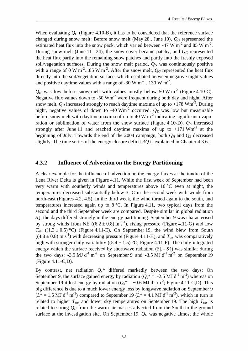
4 Results / Energy Fluxes
When evaluating QG (Figure 4.10-B), it has to be considered that the reference surface changed during snow melt: Before snow melt (May 28…June 10), QG represented the estimated heat flux into the snow pack, which varied between -47 W m-2 and 85 W m-2. During snow melt (June 11…24), the snow cover became patchy, and QG represented the heat flux partly into the remaining snow patches and partly into the freshly exposed soil/vegetation surfaces. During the snow melt period, QG was continuously positive with a range of 0 W m-2…85 W m-2. After the snow melt, QG represented the heat flux directly into the soil/vegetation surface, which oscillated between negative night values and positive daytime values with a range of -30 W m-2…130 W m-2.
QH was low before snow-melt with values mostly below 50 W m-2 (Figure 4.10-C). Negative flux values down to -50 Wm-2 were frequent during both day and night. After snow melt, QH increased strongly to reach daytime maxima of up to +178 Wm-2. During night, negative values of down to -40 Wm-2 occurred. QE was low but measurable before snow melt with daytime maxima of up to 40 W m-2 indicating significant evapo-ration or sublimation of water from the snow surface (Figure 4.10-D). QE increased strongly after June 11 and reached daytime maxima of up to +171 Wm-2 at the beginning of July. Towards the end of the 2004 campaign, both QH and QE decreased slightly. The time series of the energy closure deficit ΔQ is explained in Chapter 4.3.6.
4.3.2 Influence of Advection on the Energy Partitioning
A clear example for the influence of advection on the energy fluxes at the tundra of the Lena River Delta is given in Figure 4.11. While the first week of September had been very warm with southerly winds and temperatures above 10 °C even at night, the temperatures decreased substantially below 3 °C in the second week with winds from north-east (Figures 4.2, 4.5). In the third week, the wind turned again to the south, and temperatures increased again up to 8 °C. In Figure 4.11, two typical days from the second and the third September week are compared. Despite similar in global radiation S↓, the days differed strongly in the energy partitioning. September 9 was characterised by strong winds from NE ((6.2 ± 0.8) m s-1), rising pressure (Figure 4.11-G) and low Tair ((1.3 ± 0.5) °C) (Figure 4.11-E). On September 19, the wind blew from South ((4.8 ± 0.8) m s-1) with decreasing pressure (Figure 4.11-H), and Tair was comparatively high with stronger daily variability ((5.4 ± 1.5) °C; Figure 4.11-F). The daily-integrated energy which the surface received by shortwave radiation (S↓ - S↑) was similar during the two days: -3.9 MJ d-1 m-2 on September 9 and -3.5 MJ d-1 m-2 on September 19 (Figure 4.11-C,D).
By contrast, net radiation Qs* differed markedly between the two days: On September 9, the surface gained energy by radiation (Qs* = -2.5 MJ d-1 m-2) whereas on September 19 it lost energy by radiation (Qs* = +0.6 MJ d-1 m-2; Figure 4.11-C,D). This big difference is due to a much lower energy loss by longwave radiation on September 9 (L* = 1.5 MJ d-1 m-2) compared to September 19 (L* = 4.1 MJ d-1 m-2), which in turn is related to higher Tsur and lower sky temperatures on September 19. The high Tsur is related to strong QH from the warm air masses advected from the South to the ground surface at the investigation site. On September 19, QH was negative almost the whole
52

4 Results / Energy Fluxes
Figure 4.11. Effect of advective transport of air masses from either North or South. – Hourly means from two days in September with similar global radiation S↑ but markedly differing advective conditions are shown: A, C, E, G September 9, 2003; B, D, F, H September 19, 2003. A, Β Heat fluxes QG (—▼—), QH (—△—), QE (—○—); C, D Radiation heat fluxes Qs* (—✴—), S↓ (—▲—), S↑ (—▽—), L* (—□—); E, F Tair (—●—), VPD(—+—); G, H wind vectors ( ) and p0 (┈┈┈┈). The length of the vectors is proportional to the mean wind speed ū. The wind vectors are directed towards the reference point (zero line).
53
4 Results / Energy Fluxes
day; the daily-integrated QH was -1.6 MJ d-1 m-2. On September 9, QH was negative at night, but rose considerably above zero during midday, the daily-integrated QH was -0.7 MJ d-1 m-2. During the advection of cold air from NE on September 9, the soils were a small energy source (QG = -0.1 MJ d-1 m-2). With advection of warm air on September 19, the soils warmed up again (QG = +0.5 MJ d-1 m-2). Despite lower VPD, QE was higher on September 9 (1.1 MJ d-1 m-2) than on September 19 (0.8 MJ d-1 m-2) which is related to higher wind speed, more turbulence and thus lower aerodynamic resistance on September 9. The mean daily ra was (53 ± 6) s m-1 on September 9 and (63 ± 11) s m-1 on September 19.
4.3.3 The Diurnal Cycle of the Energy Fluxes
For the characterisation of the energy budget over the whole growing season at the wet polygonal tundra of the Lena River Delta, the energy flux data from the two campaigns 2003 and 2004 will be presented in a body from this chapter on. To improve clearness, the 2004 data will be displayed in front of the 2003 data (see also Chapter 4.1.1).
Average diurnal trends of the energy balance components for consecutive 14-days periods during the campaigns 2004 and 2003 are shown in Figure 4.12. The amount of energy which the tundra surface received by radiation (-Qs*) over the day and which was partitioned into QG, QH and QE was controlled primarily by the sun elevation and the time of the sun being above the horizon. The close relationship between sun elevation and the energy fluxes was modified considerably by environmental factors, mainly the albedo and weather conditions, i.e. cloudiness and advective conditions (see Chapter 4.3.1 and Chapter 4.3.2).
In spring and summer, a clear diurnal cycle of the energy fluxes was observed. Although the sun was continuously above the horizon, the entire sun oscillation with an elevation amplitude of 35° took place above the horizon during the polar day and could therefore cause significant variation of -Qs* and consequently also of QG, QH and QE. Following the course of the sun, the diurnal pattern of -Qs* was centred symmetrically around a midday peak which was highest in midsummer after snow melt and decreased gradually as autumn was approaching. In the night, -Qs* was regularly negative. Indeed, -Qs* already fell below zero when the sun elevation angle was below 6°…9°, thus for at least six hours per day even around midsummer. The diurnal variation of the energy fluxes weakened as the sun elevation decreased since an increasing part of the sun oscillation took place below the horizon with no direct effect on the energy fluxes at the site. At the end of the measurement period, only three to four weeks after the autumn equinox (October 12…21), a diurnal variation of the energy fluxes was hardly recognisable. The sun still spent about eight hours above the horizon but did not rise higher than 8°, so that -Qs* was continuously negative.
The increases of -Qs* in the morning resulted in associated increases of QG, QH and QE. When -Qs* reached positive values in the morning, QG also turned directly to positive values whereas QH remained negative and reached positive values only one to three hours later. Similarly, QG turned simultaneously with -Qs* to negative values in the evening while QH dropped below zero one to three hours earlier. QE was on average low
54
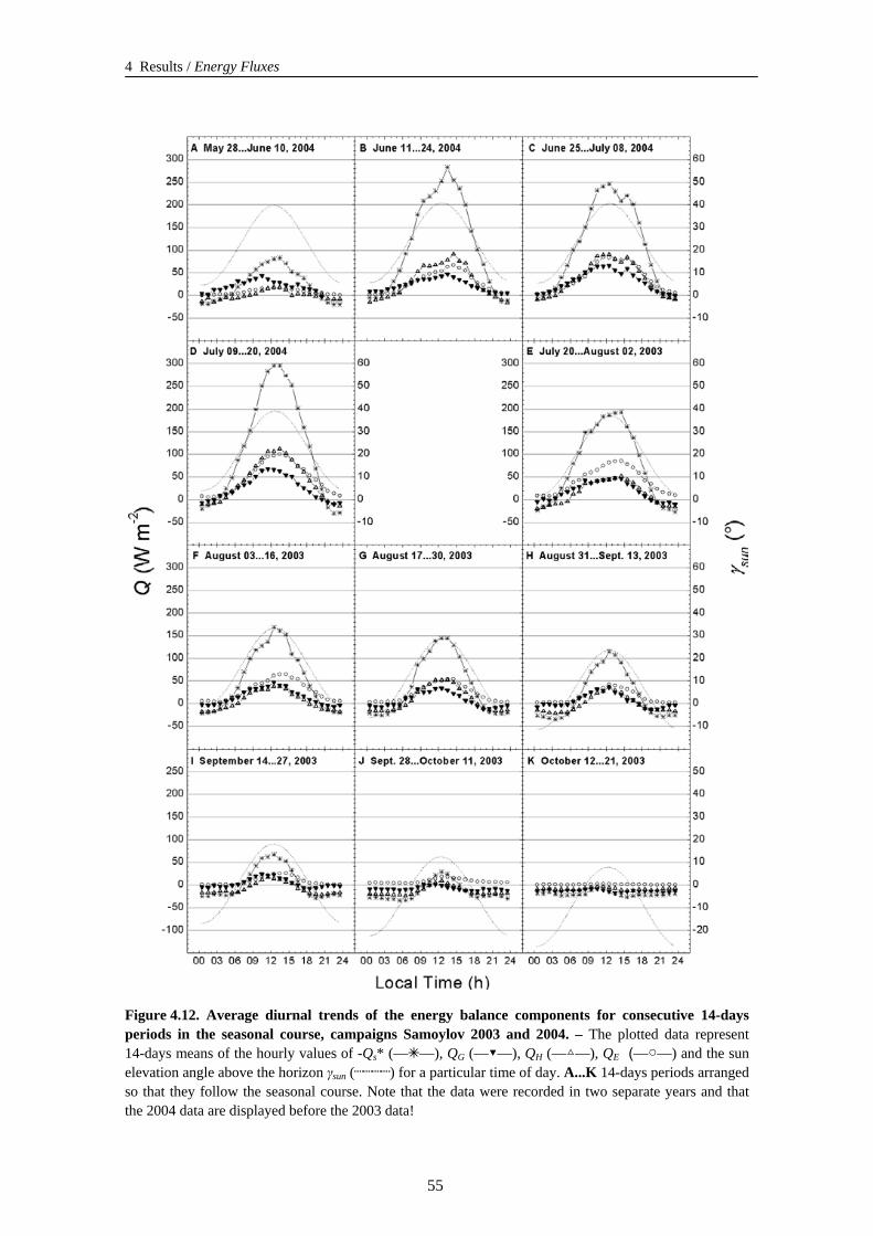
4 Results / Energy Fluxes
Figure 4.12. Average diurnal trends of the energy balance components for consecutive 14-days periods in the seasonal course, campaigns Samoylov 2003 and 2004. – The plotted data represent 14-days means of the hourly values of -Qs* (—✴—), QG (—▼—), QH (—△—), QE (—○—) and the sun elevation angle above the horizon γsun (┈┈┈┈) for a particular time of day. A...K 14-days periods arranged so that they follow the seasonal course. Note that the data were recorded in two separate years and that the 2004 data are displayed before the 2003 data!
55
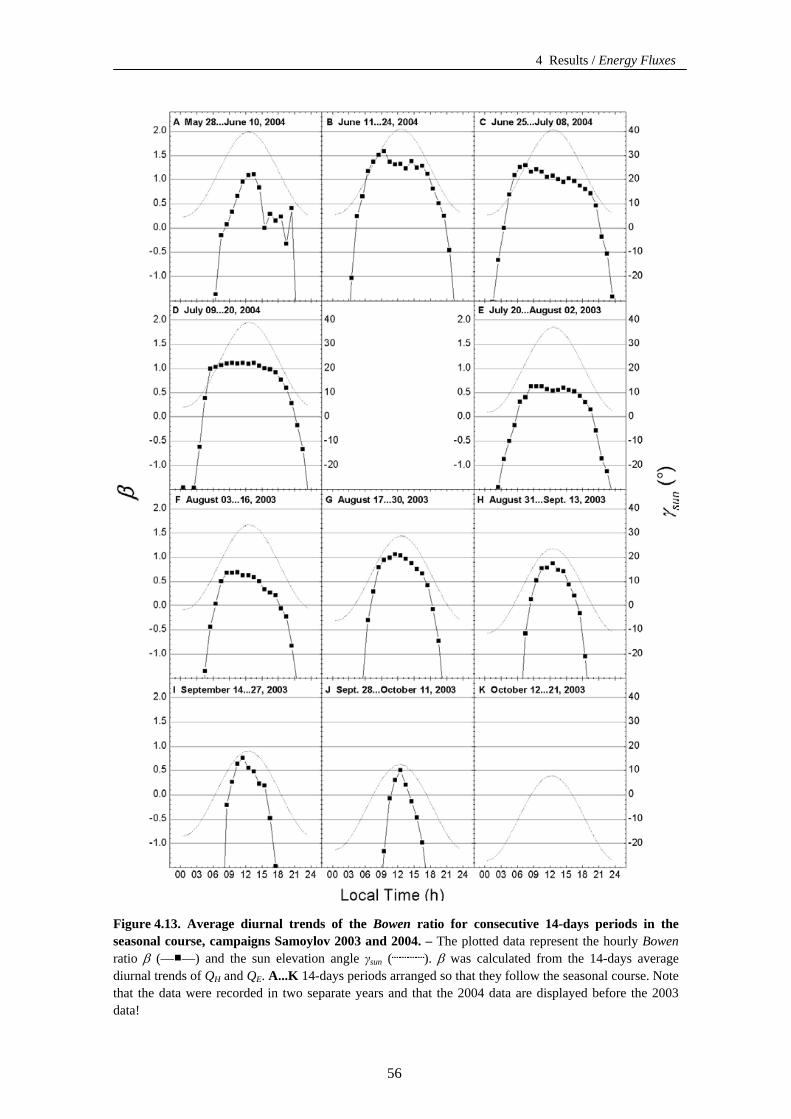
4 Results / Energy Fluxes
Figure 4.13. Average diurnal trends of the Bowen ratio for consecutive 14-days periods in the seasonal course, campaigns Samoylov 2003 and 2004. – The plotted data represent the hourly Bowen ratio β (—■—) and the sun elevation angle γsun (┈┈┈┈). β was calculated from the 14-days average diurnal trends of QH and QE. A...K 14-days periods arranged so that they follow the seasonal course. Note that the data were recorded in two separate years and that the 2004 data are displayed before the 2003 data!
56
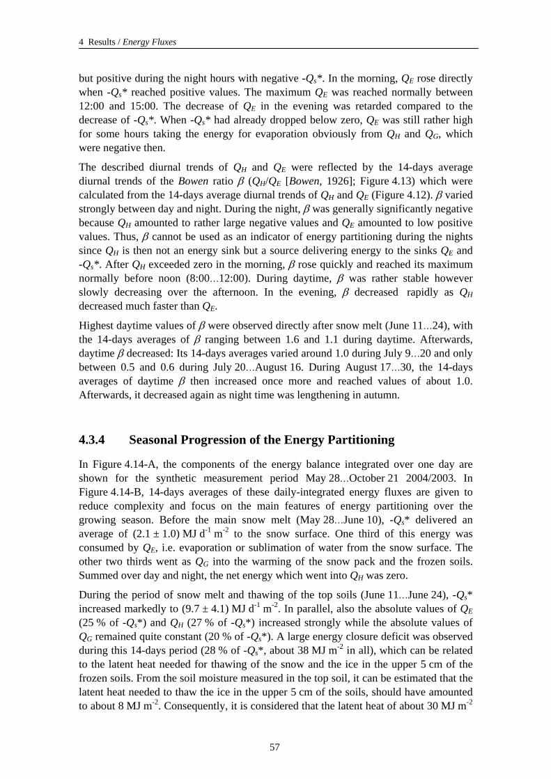
4 Results / Energy Fluxes
but positive during the night hours with negative -Qs*. In the morning, QE rose directly when -Qs* reached positive values. The maximum QE was reached normally between 12:00 and 15:00. The decrease of QE in the evening was retarded compared to the decrease of -Qs*. When -Qs* had already dropped below zero, QE was still rather high for some hours taking the energy for evaporation obviously from QH and QG, which were negative then.
The described diurnal trends of QH and QE were reflected by the 14-days average diurnal trends of the Bowen ratio β (QH/QE [Bowen, 1926]; Figure 4.13) which were calculated from the 14-days average diurnal trends of QH and QE (Figure 4.12). β varied strongly between day and night. During the night, β was generally significantly negative because QH amounted to rather large negative values and QE amounted to low positive values. Thus, β cannot be used as an indicator of energy partitioning during the nights since QH is then not an energy sink but a source delivering energy to the sinks QE and -Qs*. After QH exceeded zero in the morning, β rose quickly and reached its maximum normally before noon (8:00…12:00). During daytime, β was rather stable however slowly decreasing over the afternoon. In the evening, β decreased rapidly as QH decreased much faster than QE.
Highest daytime values of β were observed directly after snow melt (June 11…24), with the 14-days averages of β ranging between 1.6 and 1.1 during daytime. Afterwards, daytime β decreased: Its 14-days averages varied around 1.0 during July 9…20 and only between 0.5 and 0.6 during July 20…August 16. During August 17…30, the 14-days averages of daytime β then increased once more and reached values of about 1.0. Afterwards, it decreased again as night time was lengthening in autumn.
4.3.4 Seasonal Progression of the Energy Partitioning
In Figure 4.14-A, the components of the energy balance integrated over one day are shown for the synthetic measurement period May 28…October 21 2004/2003. In Figure 4.14-B, 14-days averages of these daily-integrated energy fluxes are given to reduce complexity and focus on the main features of energy partitioning over the growing season. Before the main snow melt (May 28…June 10), -Qs* delivered an average of (2.1 ± 1.0) MJ d-1 m-2 to the snow surface. One third of this energy was consumed by QE, i.e. evaporation or sublimation of water from the snow surface. The other two thirds went as QG into the warming of the snow pack and the frozen soils. Summed over day and night, the net energy which went into QH was zero.
During the period of snow melt and thawing of the top soils (June 11…June 24), -Qs* increased markedly to (9.7 ± 4.1) MJ d-1 m-2. In parallel, also the absolute values of QE (25 % of -Qs*) and QH (27 % of -Qs*) increased strongly while the absolute values of QG remained quite constant (20 % of -Qs*). A large energy closure deficit was observed during this 14-days period (28 % of -Qs*, about 38 MJ m-2 in all), which can be related to the latent heat needed for thawing of the snow and the ice in the upper 5 cm of the frozen soils. From the soil moisture measured in the top soil, it can be estimated that the latent heat needed to thaw the ice in the upper 5 cm of the soils, should have amounted to about 8 MJ m-2. Consequently, it is considered that the latent heat of about 30 MJ m-2
57
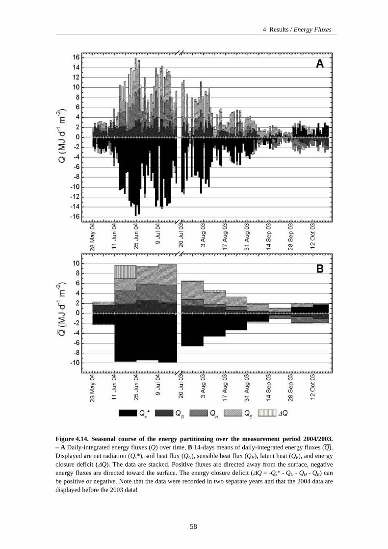
4 Results / Energy Fluxes
Figure 4.14. Seasonal course of the energy partitioning over the measurement period 2004/2003. – A Daily-integrated energy fluxes (Q) over time, B 14-days means of daily-integrated energy fluxes (Q). Displayed are net radiation (Qs*), soil heat flux (QG), sensible heat flux (QH), latent heat (QE), and energy closure deficit (ΔQ). The data are stacked. Positive fluxes are directed away from the surface, negative energy fluxes are directed toward the surface. The energy closure deficit (ΔQ = -Qs* - QG - QH - QE) can be positive or negative. Note that the data were recorded in two separate years and that the 2004 data are displayed before the 2003 data!
58
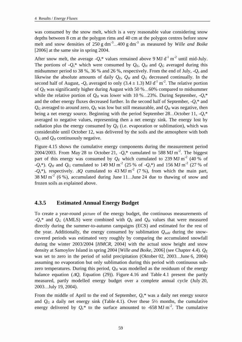
4 Results / Energy Fluxes
was consumed by the snow melt, which is a very reasonable value considering snow depths between 8 cm at the polygon rims and 40 cm at the polygon centres before snow melt and snow densities of 250 g dm-3…400 g dm-3 as measured by Wille and Boike [2006] at the same site in spring 2004.
After snow melt, the average -Qs* values remained above 9 MJ d-1 m-2 until mid-July. The portions of -Qs* which were consumed by QE, QH and QG averaged during this midsummer period to 38 %, 36 % and 26 %, respectively. From the end of July, -Qs and likewise the absolute amounts of daily QE, QH and QG decreased continually. In the second half of August, -Qs averaged to only (3.4 ± 1.3) MJ d-1 m-2. The relative portion of QE was significantly higher during August with 50 %…60% compared to midsummer while the relative portion of QH was lower with 10 %…23%. During September, -Qs* and the other energy fluxes decreased further. In the second half of September, -Qs* and QG averaged to around zero, QE was low but still measurable, and QH was negative, then being a net energy source. Beginning with the period September 28…October 11, -Qs* averaged to negative values, representing then a net energy sink. The energy lost by radiation plus the energy consumed by QE (i.e. evaporation or sublimation), which was considerable until October 12, was delivered by the soils and the atmosphere with both QG and QH continuously negative.
Figure 4.15 shows the cumulative energy components during the measurement period 2004/2003. From May 28 to October 21, -Qs* cumulated to 588 MJ m-2. The biggest part of this energy was consumed by QE which cumulated to 239 MJ m-2 (40 % of -Qs*). QH and QG cumulated to 149 MJ m-2 (25 % of -Qs*) and 156 MJ m-2 (27 % of -Qs*), respectively. ΔQ cumulated to 43 MJ m-2 (7 %), from which the main part, 38 MJ m-2 (6 %), accumulated during June 11…June 24 due to thawing of snow and frozen soils as explained above.
4.3.5 Estimated Annual Energy Budget
To create a year-round picture of the energy budget, the continuous measurements of -Qs* and QG (AMLS) were combined with QE and QH values that were measured directly during the summer-to-autumn campaigns (ECS) and estimated for the rest of the year. Additionally, the energy consumed by sublimation Qsubl during the snow-covered periods was estimated very roughly by comparing the accumulated snowfall during the winter 2003/2004 [HMCR, 2004] with the actual snow height and snow density at Samoylov Island in spring 2004 [Wille and Boike, 2006] (see Chapter 4.4). QE was set to zero in the period of solid precipitation (Oktober 02, 2003…June 6, 2004) assuming no evaporation but only sublimation during this period with continuous sub-zero temperatures. During this period, QH was modelled as the residuum of the energy balance equation (ΔQ, Equation (29)). Figure 4.16 and Table 4.1 present the partly measured, partly modelled energy budget over a complete annual cycle (July 20, 2003…July 19, 2004).
From the middle of April to the end of September, Qs* was a daily net energy source and QG a daily net energy sink (Table 4.1). Over these 5½ months, the cumulative energy delivered by Qs* to the surface amounted to -658 MJ m-2. The cumulative
59
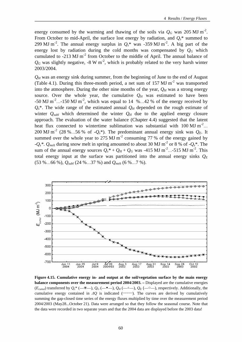
4 Results / Energy Fluxes
energy consumed by the warming and thawing of the soils via QG was 205 MJ m-2. From October to mid-April, the surface lost energy by radiation, and Qs* summed to 299 MJ m-2. The annual energy surplus in Qs* was -359 MJ m-2. A big part of the energy lost by radiation during the cold months was compensated by QG which cumulated to -213 MJ m-2 from October to the middle of April. The annual balance of QG was slightly negative, -8 W m-2, which is probably related to the very harsh winter 2003/2004.
QH was an energy sink during summer, from the beginning of June to the end of August (Table 4.1). During this three-month period, a net sum of 157 MJ m-2 was transported into the atmosphere. During the other nine months of the year, QH was a strong energy source. Over the whole year, the cumulative QH was estimated to have been -50 MJ m-2…-150 MJ m-2, which was equal to 14 %…42 % of the energy received by Qs*. The wide range of the estimated annual QH depended on the rough estimate of winter Qsubl which determined the winter QH due to the applied energy closure approach. The evaluation of the water balance (Chapter 4.4) suggested that the latent heat flux connected to wintertime sublimation was substantial with 100 MJ m-2… 200 MJ m-2 (28 %…56 % of -Qs*). The predominant annual energy sink was QE. It summed over the whole year to 275 MJ m-2 consuming 77 % of the energy gained by -Qs*. Qmelt during snow melt in spring amounted to about 30 MJ m-2 or 8 % of -Qs*. The sum of the annual energy sources Qs* + QH + QG was -415 MJ m-2…-515 MJ m-2. This total energy input at the surface was partitioned into the annual energy sinks QE (53 %…66 %), Qsubl (24 %…37 %) and Qmelt (6 %…7 %).
Figure 4.15. Cumulative energy in- and output at the soil/vegetation surface by the main energy balance components over the measurement period 2004/2003. – Displayed are the cumulative energies (Ecumul) transferred by Qs* (—✴—), QG (—▼—), QH (—△—), QE (—○—), respectively. Additionally, the cumulative energy contained in ΔQ is indicated (┈┈┈┈). The curves are derived by cumulatively summing the gap-closed time series of the energy fluxes multiplied by time over the measurement period 2004/2003 (May28...October 21). Data were arranged so that they follow the seasonal course. Note that the data were recorded in two separate years and that the 2004 data are displayed before the 2003 data!
60
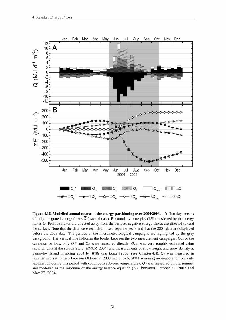
4 Results / Energy Fluxes
Figure 4.16. Modelled annual course of the energy partitioning over 2004/2003. – A Ten-days means of daily-integrated energy fluxes Q (stacked data), B cumulative energies (ΣE) transferred by the energy fluxes Q. Positive fluxes are directed away from the surface, negative energy fluxes are directed toward the surface. Note that the data were recorded in two separate years and that the 2004 data are displayed before the 2003 data! The periods of the micrometeorological campaigns are highlighted by the grey background. The vertical line indicates the border between the two measurement campaigns. Out of the campaign periods, only Qs* and QG were measured directly. Qsubl was very roughly estimated using snowfall data at the station Stolb [HMCR, 2004] and measurements of snow height and snow density at Samoylov Island in spring 2004 by Wille and Boike [2006] (see Chapter 4.4). QE was measured in summer and set to zero between Oktober 2, 2003 and June 6, 2004 assuming no evaporation but only sublimation during this period with continuous sub-zero temperatures. QH was measured during summer and modelled as the residuum of the energy balance equation (ΔQ) between October 22, 2003 and May 27, 2004.
61
4 Results / Energy Fluxes
Table 4.1. Cumulative surface energy balance components calculated over different periods within the synthetic year 2004/2003. The energy components are given as sums cumulated during the respective period. The unit for all quantities is MJ m-2 except for the relative fractions Qx /-Qs*. Modelled values are presented in italics, measured values are presented in normal font.
Jun 01…Aug 31 April 15…Sep 28 Jan 01…Dez 31 summer period of positive
daily –Qs* whole year
Extraterrestrial solar radiation ETSR -3355 -5239 -5950
Global radiation S↓ -1423 n.d. n.d.
Absorbed global radiation S↓ + S↑ -1049 n.d. n.d.
Albedo α 0.26 n.d. n.d.
Long-wave incoming radiation L↓ -2337 n.d. n.d.
Long-wave outgoing radiation L↑B (L↑B A) 2772 (2745) 4669 8228
Long-wave net radiation L* = L↓ + L↑B 435 n.d. n.d.
Net radiation Qs* AMLS (ECS) -607 (-641) -658 -359
Ground heat flux polygon rim QG-rim 176 238 -4
Ground heat flux polygon centre QG-centre 151 174 -12
Mean ground heat flux QG 163 205 -8
Sensible Heat Flux QH 157 n.d. -50…-150
Latent Heat Flux QE 250 n.d. 275
Estimated Qsubl (sublimation heat flux) - n.d. 100…200
Latent heat of snow melt Qmelt 30 30 30
QG /-Qs* 0.25 0.31 -0.02
QH /-Qs* 0.26 n.d. -0.14…-0.42
QE / -Qs* 0.41 n.d. 0.77
Qsubl / -Qs - n.d. 0.28…0.56
Qmelt /-Qs* 0.05 0.05 0.08
62
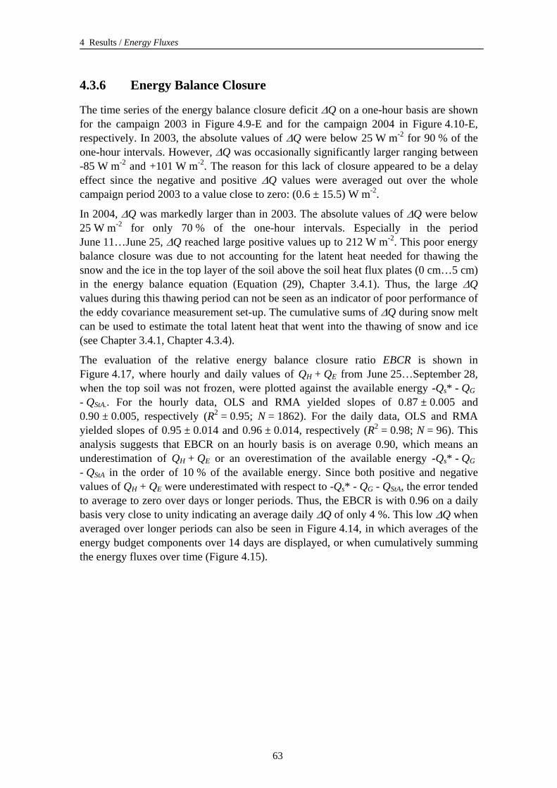
4 Results / Energy Fluxes
4.3.6 Energy Balance Closure
The time series of the energy balance closure deficit ΔQ on a one-hour basis are shown for the campaign 2003 in Figure 4.9-E and for the campaign 2004 in Figure 4.10-E, respectively. In 2003, the absolute values of ΔQ were below 25 W m-2 for 90 % of the one-hour intervals. However, ΔQ was occasionally significantly larger ranging between -85 W m-2 and +101 W m-2. The reason for this lack of closure appeared to be a delay effect since the negative and positive ΔQ values were averaged out over the whole campaign period 2003 to a value close to zero: (0.6 ± 15.5) W m-2.
In 2004, ΔQ was markedly larger than in 2003. The absolute values of ΔQ were below 25 W m-2 for only 70 % of the one-hour intervals. Especially in the period June 11…June 25, ΔQ reached large positive values up to 212 W m-2. This poor energy balance closure was due to not accounting for the latent heat needed for thawing the snow and the ice in the top layer of the soil above the soil heat flux plates (0 cm…5 cm) in the energy balance equation (Equation (29), Chapter 3.4.1). Thus, the large ΔQ values during this thawing period can not be seen as an indicator of poor performance of the eddy covariance measurement set-up. The cumulative sums of ΔQ during snow melt can be used to estimate the total latent heat that went into the thawing of snow and ice (see Chapter 3.4.1, Chapter 4.3.4).
The evaluation of the relative energy balance closure ratio EBCR is shown in Figure 4.17, where hourly and daily values of QH + QE from June 25…September 28, when the top soil was not frozen, were plotted against the available energy -Qs* - QG - QStA.. For the hourly data, OLS and RMA yielded slopes of 0.87 ± 0.005 and 0.90 ± 0.005, respectively (R2 = 0.95; N = 1862). For the daily data, OLS and RMA yielded slopes of 0.95 ± 0.014 and 0.96 ± 0.014, respectively (R2 = 0.98; N = 96). This analysis suggests that EBCR on an hourly basis is on average 0.90, which means an underestimation of QH + QE or an overestimation of the available energy -Qs* - QG - QStA in the order of 10 % of the available energy. Since both positive and negative values of QH + QE were underestimated with respect to -Qs* - QG - QStA, the error tended to average to zero over days or longer periods. Thus, the EBCR is with 0.96 on a daily basis very close to unity indicating an average daily ΔQ of only 4 %. This low ΔQ when averaged over longer periods can also be seen in Figure 4.14, in which averages of the energy budget components over 14 days are displayed, or when cumulatively summing the energy fluxes over time (Figure 4.15).
63
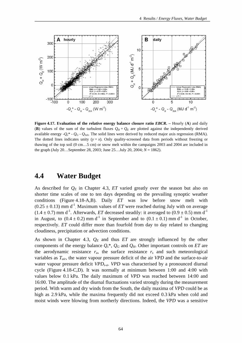
4 Results / Energy Fluxes, Water Budget
Figure 4.17. Evaluation of the relative energy balance closure ratio EBCR. – Hourly (A) and daily (B) values of the sum of the turbulent fluxes QH + QE are plotted against the independently derived available energy -Qs* - QG - QStA. The solid lines were derived by reduced major axis regression (RMA). The dotted lines indicates unity (y = x). Only quality-screened data from periods without freezing or thawing of the top soil (0 cm…5 cm) or snow melt within the campaigns 2003 and 2004 are included in the graph (July 20…September 28, 2003; June 25…July 20, 2004; N = 1862).
4.4 Water Budget As described for QE in Chapter 4.3, ET varied greatly over the season but also on shorter time scales of one to ten days depending on the prevailing synoptic weather conditions (Figure 4.18-A,B). Daily ET was low before snow melt with (0.25 ± 0.13) mm d-1
. Maximum values of ET were reached during July with on average (1.4 ± 0.7) mm d-1. Afterwards, ET decreased steadily: it averaged to (0.9 ± 0.5) mm d-1 in August, to (0.4 ± 0.2) mm d-1 in September and to (0.1 ± 0.1) mm d-1 in October, respectively. ET could differ more than fourfold from day to day related to changing cloudiness, precipitation or advection conditions.
As shown in Chapter 4.3, QE and thus ET are strongly influenced by the other components of the energy balance Qs*, QG and QH. Other important controls on ET are the aerodynamic resistance ra, the surface resistance rs and such meteorological variables as Tair, the water vapour pressure deficit of the air VPD and the surface-to-air water vapour pressure deficit VPDs-a. VPD was characterised by a pronounced diurnal cycle (Figure 4.18-C,D). It was normally at minimum between 1:00 and 4:00 with values below 0.1 kPa. The daily maximum of VPD was reached between 14:00 and 16:00. The amplitude of the diurnal fluctuations varied strongly during the measurement period. With warm and dry winds from the South, the daily maxima of VPD could be as high as 2.9 kPa, while the maxima frequently did not exceed 0.3 kPa when cold and moist winds were blowing from northerly directions. Indeed, the VPD was a sensitive
64
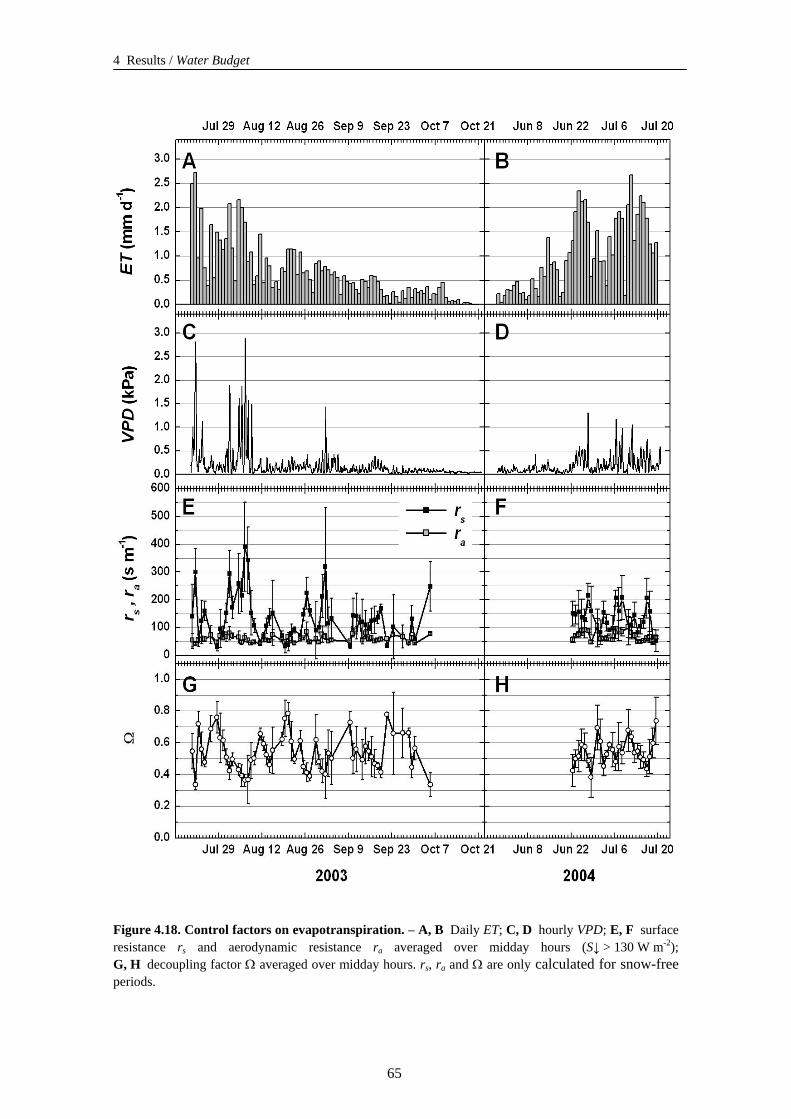
4 Results / Water Budget
Figure 4.18. Control factors on evapotranspiration. – A, B Daily ET; C, D hourly VPD; E, F surface resistance rs and aerodynamic resistance ra averaged over midday hours (S↓ > 130 W m-2); G, H decoupling factor Ω averaged over midday hours. rs, ra and Ω are only calculated for snow-free periods.
65
4 Results / Water Budget
indicator of the respective advective conditions. In Figure 4.18, midday (S↓ > 130 W m-2) averages of aerodynamic resistance ra, surface resistance rs (E,F) and the decoupling factor Ω (G,H) are presented for the snow-free periods. The hourly values (not shown) of midday ra varied between 32 s m-1 and 133 s m-1 with a mean of (62 ± 18) s m-1 (median: 58 s m-1). The hourly values (not shown) of midday rs were larger than ra and showed a wider variation. They ranged between 6 and 673 s m-1 with a mean of (143 ± 94) s m-1 (median: 121 s m-1). Variations in average midday rs were significantly correlated to variations in the surface-to-air water vapour pressure deficit VPDs-a (R = 0.89; Figure 4.19). During the period July 20…August 31, rs increased linearly with increasing VPDs-a. Calculated over longer periods, the relation weakened, probably because it was masked by the effects of the phenological changes of the canopy over the season. The hourly midday values of the decoupling factor Ω ranged between 0.19 and 0.95 with a mean of 0.53 ± 0.13 (median: 0.52). During advection of warm and dry air from the South, VPD was high which forced rs to increase distinctly above 100 s m-1and Ω to decrease below 0.5. An Ω below 0.5 indicates that ET is more limited by the interplay of surface resistance and atmospheric conditions (windspeed, VPD) than by the available energy -Qs* - QG - QStA. During advection of cold and moist air, VPD was low and rs was below 100 s m-1. Ω was above 0.5 indicating less coupling of vegetation and atmosphere; ET was then mainly controlled by the available energy.
Figure 4.19. Relationship between surface resistance rs and surface-to-air water vapour pressure deficit VPDs-a. – The data points represent midday averages from the period July 20…August 31, 2003. Midday is here defined as hourly intervals with S↓ > 130 W m-2. The calculation of VPDs-a is described in Chapter 3.4.2.
66
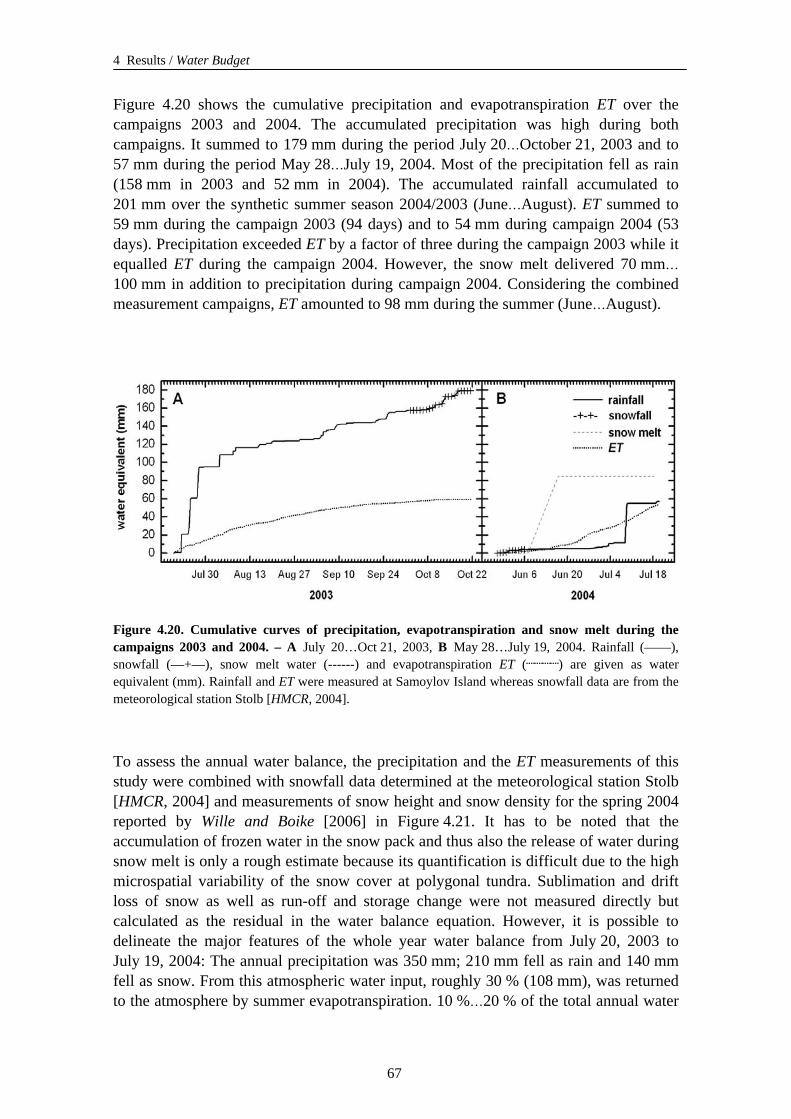
4 Results / Water Budget
Figure 4.20 shows the cumulative precipitation and evapotranspiration ET over the campaigns 2003 and 2004. The accumulated precipitation was high during both campaigns. It summed to 179 mm during the period July 20…October 21, 2003 and to 57 mm during the period May 28…July 19, 2004. Most of the precipitation fell as rain (158 mm in 2003 and 52 mm in 2004). The accumulated rainfall accumulated to 201 mm over the synthetic summer season 2004/2003 (June…August). ET summed to 59 mm during the campaign 2003 (94 days) and to 54 mm during campaign 2004 (53 days). Precipitation exceeded ET by a factor of three during the campaign 2003 while it equalled ET during the campaign 2004. However, the snow melt delivered 70 mm… 100 mm in addition to precipitation during campaign 2004. Considering the combined measurement campaigns, ET amounted to 98 mm during the summer (June…August).
Figure 4.20. Cumulative curves of precipitation, evapotranspiration and snow melt during the campaigns 2003 and 2004. – A July 20…Oct 21, 2003, B May 28…July 19, 2004. Rainfall (——), snowfall (—+—), snow melt water (------) and evapotranspiration ET (┈┈┈┈) are given as water equivalent (mm). Rainfall and ET were measured at Samoylov Island whereas snowfall data are from the meteorological station Stolb [HMCR, 2004].
To assess the annual water balance, the precipitation and the ET measurements of this study were combined with snowfall data determined at the meteorological station Stolb [HMCR, 2004] and measurements of snow height and snow density for the spring 2004 reported by Wille and Boike [2006] in Figure 4.21. It has to be noted that the accumulation of frozen water in the snow pack and thus also the release of water during snow melt is only a rough estimate because its quantification is difficult due to the high microspatial variability of the snow cover at polygonal tundra. Sublimation and drift loss of snow as well as run-off and storage change were not measured directly but calculated as the residual in the water balance equation. However, it is possible to delineate the major features of the whole year water balance from July 20, 2003 to July 19, 2004: The annual precipitation was 350 mm; 210 mm fell as rain and 140 mm fell as snow. From this atmospheric water input, roughly 30 % (108 mm), was returned to the atmosphere by summer evapotranspiration. 10 %…20 % of the total annual water
67
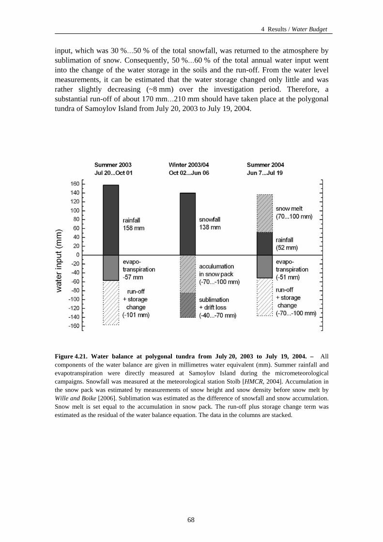
4 Results / Water Budget
input, which was 30 %…50 % of the total snowfall, was returned to the atmosphere by sublimation of snow. Consequently, 50 %…60 % of the total annual water input went into the change of the water storage in the soils and the run-off. From the water level measurements, it can be estimated that the water storage changed only little and was rather slightly decreasing (~8 mm) over the investigation period. Therefore, a substantial run-off of about 170 mm…210 mm should have taken place at the polygonal tundra of Samoylov Island from July 20, 2003 to July 19, 2004.
Figure 4.21. Water balance at polygonal tundra from July 20, 2003 to July 19, 2004. – All components of the water balance are given in millimetres water equivalent (mm). Summer rainfall and evapotranspiration were directly measured at Samoylov Island during the micrometeorological campaigns. Snowfall was measured at the meteorological station Stolb [HMCR, 2004]. Accumulation in the snow pack was estimated by measurements of snow height and snow density before snow melt by Wille and Boike [2006]. Sublimation was estimated as the difference of snowfall and snow accumulation. Snow melt is set equal to the accumulation in snow pack. The run-off plus storage change term was estimated as the residual of the water balance equation. The data in the columns are stacked.
68
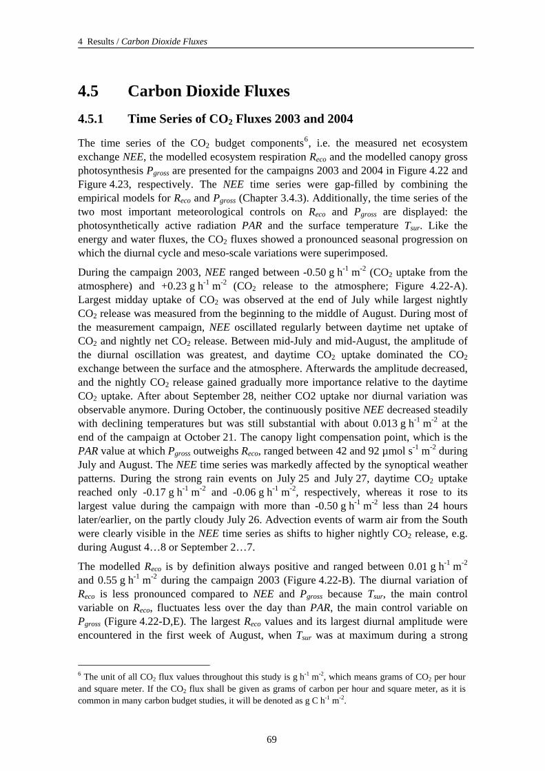
4 Results / Carbon Dioxide Fluxes
4.5 Carbon Dioxide Fluxes 4.5.1 Time Series of CO2 Fluxes 2003 and 2004
The time series of the CO2 budget components6, i.e. the measured net ecosystem exchange NEE, the modelled ecosystem respiration Reco and the modelled canopy gross photosynthesis Pgross are presented for the campaigns 2003 and 2004 in Figure 4.22 and Figure 4.23, respectively. The NEE time series were gap-filled by combining the empirical models for Reco and Pgross (Chapter 3.4.3). Additionally, the time series of the two most important meteorological controls on Reco and Pgross are displayed: the photosynthetically active radiation PAR and the surface temperature Tsur. Like the energy and water fluxes, the CO2 fluxes showed a pronounced seasonal progression on which the diurnal cycle and meso-scale variations were superimposed.
During the campaign 2003, NEE ranged between -0.50 g h-1 m-2 (CO2 uptake from the atmosphere) and +0.23 g h-1 m-2 (CO2 release to the atmosphere; Figure 4.22-A). Largest midday uptake of CO2 was observed at the end of July while largest nightly CO2 release was measured from the beginning to the middle of August. During most of the measurement campaign, NEE oscillated regularly between daytime net uptake of CO2 and nightly net CO2 release. Between mid-July and mid-August, the amplitude of the diurnal oscillation was greatest, and daytime CO2 uptake dominated the CO2 exchange between the surface and the atmosphere. Afterwards the amplitude decreased, and the nightly CO2 release gained gradually more importance relative to the daytime CO2 uptake. After about September 28, neither CO2 uptake nor diurnal variation was observable anymore. During October, the continuously positive NEE decreased steadily with declining temperatures but was still substantial with about 0.013 g h-1 m-2 at the end of the campaign at October 21. The canopy light compensation point, which is the PAR value at which Pgross outweighs Reco, ranged between 42 and 92 µmol s-1 m-2 during July and August. The NEE time series was markedly affected by the synoptical weather patterns. During the strong rain events on July 25 and July 27, daytime CO2 uptake reached only -0.17 g h-1 m-2 and -0.06 g h-1 m-2, respectively, whereas it rose to its largest value during the campaign with more than -0.50 g h-1 m-2 less than 24 hours later/earlier, on the partly cloudy July 26. Advection events of warm air from the South were clearly visible in the NEE time series as shifts to higher nightly CO2 release, e.g. during August 4…8 or September 2…7.
The modelled Reco is by definition always positive and ranged between 0.01 g h-1 m-2 and 0.55 g h-1 m-2 during the campaign 2003 (Figure 4.22-B). The diurnal variation of Reco is less pronounced compared to NEE and Pgross because Tsur, the main control variable on Reco, fluctuates less over the day than PAR, the main control variable on Pgross (Figure 4.22-D,E). The largest Reco values and its largest diurnal amplitude were encountered in the first week of August, when Tsur was at maximum during a strong
6 The unit of all CO2 flux values throughout this study is g h-1 m-2, which means grams of CO2 per hour and square meter. If the CO2 flux shall be given as grams of carbon per hour and square meter, as it is common in many carbon budget studies, it will be denoted as g C h-1 m-2.
69
4 Resultss / Carbon Dioxide Fluxes
advection event of warm air from the south. The mean Reco during August 4...8 was (0.23 ± 0.10) g h-1 m-2. Afterwards, Reco decreased with approaching autumn; it averaged to (0.11 ± 0.03) g h-1 m-2 during August 9…31, to (0.09 ± 0.03) g h-1 m-2 during September and to (0.03 ± 0.01) g h-1 m-2 during October.
The modelled Pgross is by definition always negative and ranged between zero and -0.70 g h-1 m-2 during the campaign 2003 (Figure 4.22-C). Following the daily trend of PAR, the amplitude of the diurnal oscillation of Pgross is large. From the beginning of measurements until about August 10, photosynthesis took place for 24 hours per day, however, with only small absolute values during the night hours. The largest absolute
Figure 4.22. Time series of CO2 budget components and meteorological controls, 2003. – A NEE measured by the eddy covariance method; B modelled Reco; C modelled Pgross (solid line) and gross photosynthesis near light saturation Pn-sat (dotted line); D photosynthetically active radiation PAR (main control on Pgross); E surface temperature Tsur (main control on Reco).
70
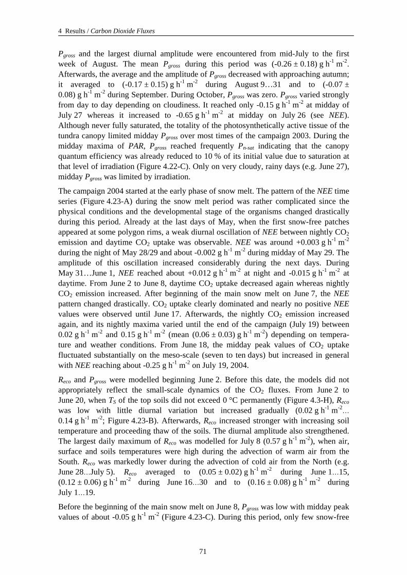
4 Results / Carbon Dioxide Fluxes
Pgross and the largest diurnal amplitude were encountered from mid-July to the first week of August. The mean Pgross during this period was (-0.26 ± 0.18) g h-1 m-2. Afterwards, the average and the amplitude of Pgross decreased with approaching autumn; it averaged to (-0.17 ± 0.15) g h-1 m-2 during August 9…31 and to (-0.07 ± 0.08) g h-1 m-2 during September. During October, Pgross was zero. Pgross varied strongly from day to day depending on cloudiness. It reached only -0.15 g h-1 m-2 at midday of July 27 whereas it increased to -0.65 g h-1 m-2 at midday on July 26 (see NEE). Although never fully saturated, the totality of the photosynthetically active tissue of the tundra canopy limited midday Pgross over most times of the campaign 2003. During the midday maxima of PAR, Pgross reached frequently Pn-sat indicating that the canopy quantum efficiency was already reduced to 10 % of its initial value due to saturation at that level of irradiation (Figure 4.22-C). Only on very cloudy, rainy days (e.g. June 27), midday Pgross was limited by irradiation.
The campaign 2004 started at the early phase of snow melt. The pattern of the NEE time series (Figure 4.23-A) during the snow melt period was rather complicated since the physical conditions and the developmental stage of the organisms changed drastically during this period. Already at the last days of May, when the first snow-free patches appeared at some polygon rims, a weak diurnal oscillation of NEE between nightly CO2 emission and daytime CO2 uptake was observable. NEE was around +0.003 g h-1 m-2 during the night of May 28/29 and about -0.002 g h-1 m-2 during midday of May 29. The amplitude of this oscillation increased considerably during the next days. During May 31…June 1, NEE reached about +0.012 g h-1 m-2 at night and -0.015 g h-1 m-2 at daytime. From June 2 to June 8, daytime CO2 uptake decreased again whereas nightly CO2 emission increased. After beginning of the main snow melt on June 7, the NEE pattern changed drastically. CO2 uptake clearly dominated and nearly no positive NEE values were observed until June 17. Afterwards, the nightly CO2 emission increased again, and its nightly maxima varied until the end of the campaign (July 19) between 0.02 g h-1 m-2 and 0.15 g h-1 m-2 (mean (0.06 ± 0.03) g h-1 m-2) depending on tempera-ture and weather conditions. From June 18, the midday peak values of CO2 uptake fluctuated substantially on the meso-scale (seven to ten days) but increased in general with NEE reaching about -0.25 g h-1 m-2 on July 19, 2004.
Reco and Pgross were modelled beginning June 2. Before this date, the models did not appropriately reflect the small-scale dynamics of the CO2 fluxes. From June 2 to June 20, when TS of the top soils did not exceed 0 °C permanently (Figure 4.3-H), Reco was low with little diurnal variation but increased gradually (0.02 g h-1 m-2… 0.14 g h-1 m-2; Figure 4.23-B). Afterwards, Reco increased stronger with increasing soil temperature and proceeding thaw of the soils. The diurnal amplitude also strengthened. The largest daily maximum of Reco was modelled for July 8 (0.57 g h-1 m-2), when air, surface and soils temperatures were high during the advection of warm air from the South. Reco was markedly lower during the advection of cold air from the North (e.g. June 28…July 5). Reco averaged to (0.05 ± 0.02) g h-1 m-2 during June 1…15, (0.12 ± 0.06) g h-1 m-2 during June 16…30 and to (0.16 ± 0.08) g h-1 m-2 during July 1…19.
Before the beginning of the main snow melt on June 8, Pgross was low with midday peak values of about -0.05 g h-1 m-2 (Figure 4.23-C). During this period, only few snow-free
71
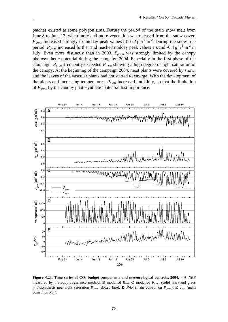
4 Resultss / Carbon Dioxide Fluxes
patches existed at some polygon rims. During the period of the main snow melt from June 8 to June 17, when more and more vegetation was released from the snow cover, Pgross increased strongly to midday peak values of -0.2 g h-1 m-2. During the snow-free period, Pgross increased further and reached midday peak values around -0.4 g h-1 m-2 in July. Even more distinctly than in 2003, Pgross was strongly limited by the canopy photosynthetic potential during the campaign 2004. Especially in the first phase of the campaign, Pgross frequently exceeded Pn-sat showing a high degree of light saturation of the canopy. At the beginning of the campaign 2004, most plants were covered by snow, and the leaves of the vascular plants had not started to emerge. With the development of the plants and increasing temperatures, Pn-sat increased until July, so that the limitation of Pgross by the canopy photosynthetic potential lost importance.
Figure 4.23. Time series of CO2 budget components and meteorological controls, 2004. – A NEE measured by the eddy covariance method; B modelled Reco; C modelled Pgross (solid line) and gross photosynthesis near light saturation Pn-sat (dotted line); D PAR (main control on Pgross); E Tsur (main control on Reco).
72
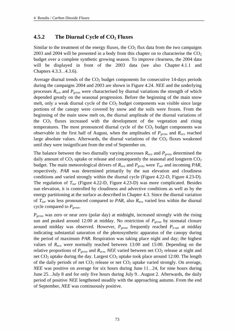
4 Results / Carbon Dioxide Fluxes
4.5.2 The Diurnal Cycle of CO2 Fluxes
Similar to the treatment of the energy fluxes, the CO2 flux data from the two campaigns 2003 and 2004 will be presented in a body from this chapter on to characterise the CO2 budget over a complete synthetic growing season. To improve clearness, the 2004 data will be displayed in front of the 2003 data (see also Chapter 4.1.1 and Chapters 4.3.3…4.3.6).
Average diurnal trends of the CO2 budget components for consecutive 14-days periods during the campaigns 2004 and 2003 are shown in Figure 4.24. NEE and the underlying processes Reco and Pgross were characterised by diurnal variations the strength of which depended greatly on the seasonal progression. Before the beginning of the main snow melt, only a weak diurnal cycle of the CO2 budget components was visible since large portions of the canopy were covered by snow and the soils were frozen. From the beginning of the main snow melt on, the diurnal amplitude of the diurnal variations of the CO2 fluxes increased with the development of the vegetation and rising temperatures. The most pronounced diurnal cycle of the CO2 budget components was observable in the first half of August, when the amplitudes of Pgross and Reco reached large absolute values. Afterwards, the diurnal variations of the CO2 fluxes weakened until they were insignificant from the end of September on.
The balance between the two diurnally varying processes Reco and Pgross determined the daily amount of CO2 uptake or release and consequently the seasonal and longterm CO2 budget. The main meteorological drivers of Reco and Pgross were Tsur and incoming PAR, respectively. PAR was determined primarily by the sun elevation and cloudiness conditions and varied strongly within the diurnal cycle (Figure 4.22-D, Figure 4.23-D). The regulation of Tsur (Figure 4.22-D, Figure 4.23-D) was more complicated. Besides sun elevation, it is controlled by cloudiness and advective conditions as well as by the energy partitioning at the surface as described in Chapter 4.3. Since the diurnal variation of Tsur was less pronounced compared to PAR, also Reco varied less within the diurnal cycle compared to Pgross.
Pgross was zero or near zero (polar day) at midnight, increased strongly with the rising sun and peaked around 12:00 at midday. No restriction of Pgross by stomatal closure around midday was observed. However, Pgross frequently reached Pn-sat at midday indicating substantial saturation of the photosynthetic apparatus of the canopy during the period of maximum PAR. Respiration was taking place night and day; the highest values of Reco were normally reached between 13:00 and 15:00. Depending on the relative proportions of Pgross and Reco, NEE varied between net CO2 release at night and net CO2 uptake during the day. Largest CO2 uptake took place around 12:00. The length of the daily periods of net CO2 release or net CO2 uptake varied strongly. On average, NEE was positive on average for six hours during June 11…24, for nine hours during June 25…July 8 and for only five hours during July 9…August 2. Afterwards, the daily period of positive NEE lengthened steadily with the approaching autumn. From the end of September, NEE was continuously positive.
73
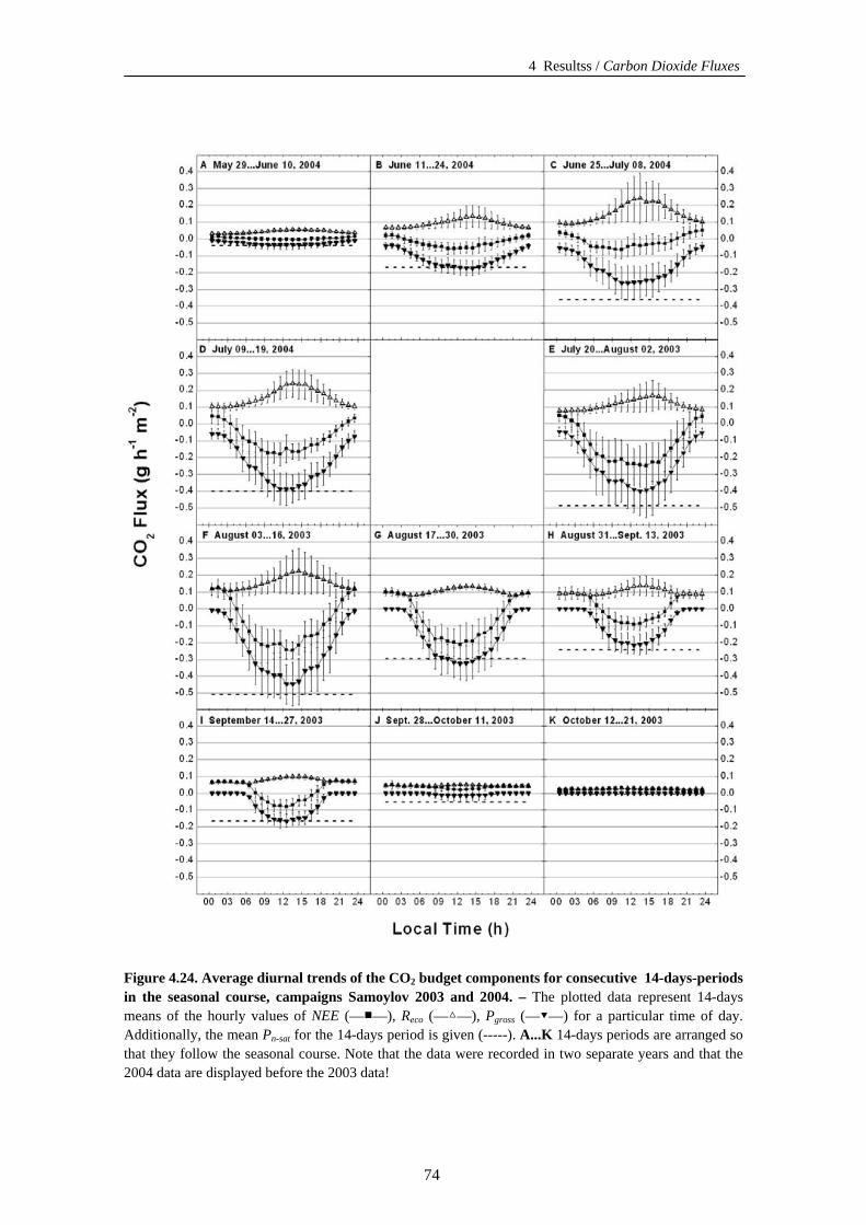
4 Resultss / Carbon Dioxide Fluxes
Figure 4.24. Average diurnal trends of the CO2 budget components for consecutive 14-days-periods in the seasonal course, campaigns Samoylov 2003 and 2004. – The plotted data represent 14-days means of the hourly values of NEE (—■—), Reco (—△—), Pgross (—▼—) for a particular time of day. Additionally, the mean Pn-sat for the 14-days period is given (-----). A...K 14-days periods are arranged so that they follow the seasonal course. Note that the data were recorded in two separate years and that the 2004 data are displayed before the 2003 data!
74
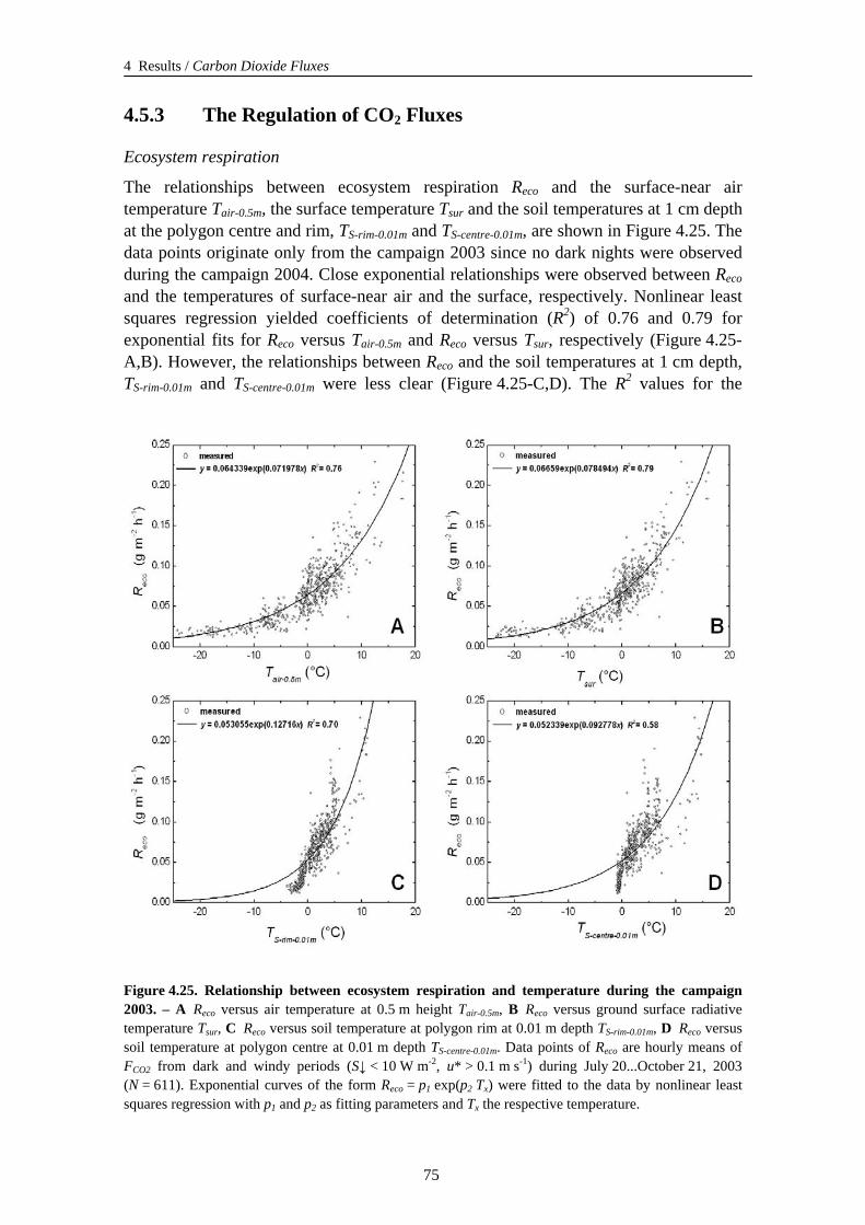
4 Results / Carbon Dioxide Fluxes
4.5.3 The Regulation of CO2 Fluxes
Ecosystem respiration
The relationships between ecosystem respiration Reco and the surface-near air temperature Tair-0.5m, the surface temperature Tsur and the soil temperatures at 1 cm depth at the polygon centre and rim, TS-rim-0.01m and TS-centre-0.01m, are shown in Figure 4.25. The data points originate only from the campaign 2003 since no dark nights were observed during the campaign 2004. Close exponential relationships were observed between Reco and the temperatures of surface-near air and the surface, respectively. Nonlinear least squares regression yielded coefficients of determination (R2) of 0.76 and 0.79 for exponential fits for Reco versus Tair-0.5m and Reco versus Tsur, respectively (Figure 4.25-A,B). However, the relationships between Reco and the soil temperatures at 1 cm depth, TS-rim-0.01m and TS-centre-0.01m were less clear (Figure 4.25-C,D). The R2 values for the
Figure 4.25. Relationship between ecosystem respiration and temperature during the campaign 2003. – A Reco versus air temperature at 0.5 m height Tair-0.5m, B Reco versus ground surface radiative temperature Tsur, C Reco versus soil temperature at polygon rim at 0.01 m depth TS-rim-0.01m, D Reco versus soil temperature at polygon centre at 0.01 m depth TS-centre-0.01m. Data points of Reco are hourly means of FCO2 from dark and windy periods (S↓ < 10 W m-2, u* > 0.1 m s-1) during July 20...October 21, 2003 (N = 611). Exponential curves of the form Reco = p1 exp(p2 Tx) were fitted to the data by nonlinear least squares regression with p1 and p2 as fitting parameters and Tx the respective temperature.
75
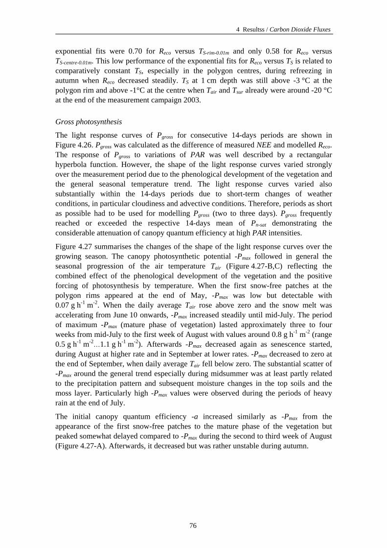
4 Resultss / Carbon Dioxide Fluxes
exponential fits were 0.70 for Reco versus TS-rim-0.01m and only 0.58 for Reco versus TS-centre-0.01m. This low performance of the exponential fits for Reco versus TS is related to comparatively constant TS, especially in the polygon centres, during refreezing in autumn when Reco decreased steadily. TS at 1 cm depth was still above -3 °C at the polygon rim and above -1°C at the centre when Tair and Tsur already were around -20 °C at the end of the measurement campaign 2003.
Gross photosynthesis
The light response curves of Pgross for consecutive 14-days periods are shown in Figure 4.26. Pgross was calculated as the difference of measured NEE and modelled Reco. The response of Pgross to variations of PAR was well described by a rectangular hyperbola function. However, the shape of the light response curves varied strongly over the measurement period due to the phenological development of the vegetation and the general seasonal temperature trend. The light response curves varied also substantially within the 14-days periods due to short-term changes of weather conditions, in particular cloudiness and advective conditions. Therefore, periods as short as possible had to be used for modelling Pgross (two to three days). Pgross frequently reached or exceeded the respective 14-days mean of Pn-sat demonstrating the considerable attenuation of canopy quantum efficiency at high PAR intensities.
Figure 4.27 summarises the changes of the shape of the light response curves over the growing season. The canopy photosynthetic potential -Pmax followed in general the seasonal progression of the air temperature Tair (Figure 4.27-B,C) reflecting the combined effect of the phenological development of the vegetation and the positive forcing of photosynthesis by temperature. When the first snow-free patches at the polygon rims appeared at the end of May, -Pmax was low but detectable with 0.07 g h-1 m-2. When the daily average Tair rose above zero and the snow melt was accelerating from June 10 onwards, -Pmax increased steadily until mid-July. The period of maximum -Pmax (mature phase of vegetation) lasted approximately three to four weeks from mid-July to the first week of August with values around 0.8 g h-1 m-2 (range 0.5 g h-1 m-2…1.1 g h-1 m-2). Afterwards -Pmax decreased again as senescence started, during August at higher rate and in September at lower rates. -Pmax decreased to zero at the end of September, when daily average Tair fell below zero. The substantial scatter of -Pmax around the general trend especially during midsummer was at least partly related to the precipitation pattern and subsequent moisture changes in the top soils and the moss layer. Particularly high -Pmax values were observed during the periods of heavy rain at the end of July.
The initial canopy quantum efficiency -a increased similarly as -Pmax from the appearance of the first snow-free patches to the mature phase of the vegetation but peaked somewhat delayed compared to -Pmax during the second to third week of August (Figure 4.27-A). Afterwards, it decreased but was rather unstable during autumn.
76
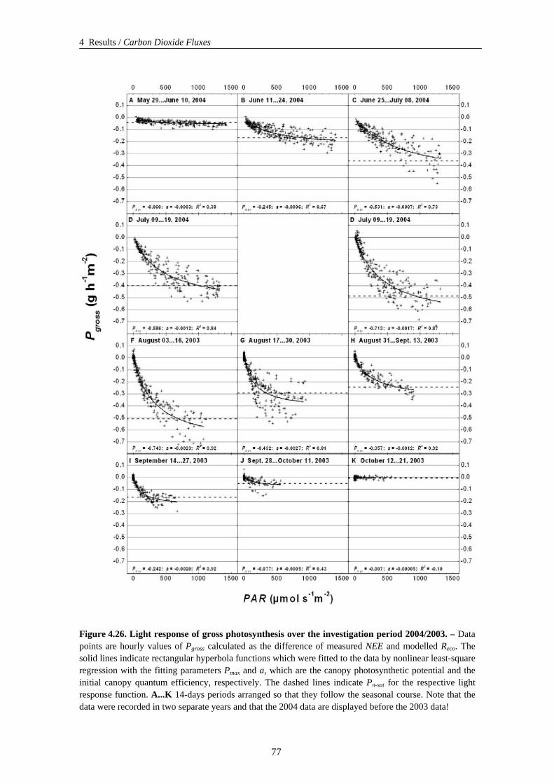
4 Results / Carbon Dioxide Fluxes
Figure 4.26. Light response of gross photosynthesis over the investigation period 2004/2003. – Data points are hourly values of Pgross calculated as the difference of measured NEE and modelled Reco. The solid lines indicate rectangular hyperbola functions which were fitted to the data by nonlinear least-square regression with the fitting parameters Pmax and a, which are the canopy photosynthetic potential and the initial canopy quantum efficiency, respectively. The dashed lines indicate Pn-sat for the respective light response function. A...K 14-days periods arranged so that they follow the seasonal course. Note that the data were recorded in two separate years and that the 2004 data are displayed before the 2003 data!
77
4 Resultss / Carbon Dioxide Fluxes
Figure 4.27. Seasonal progression of initial canopy quantum efficiency a and canopy photosynthetic potential Pmax. – A Initial canopy quantum efficiency –a, B canopy photosynthetic potential –Pmax; C average air temperature Tair-B. Data points were calculated over two-days periods in 2003 and over three-days periods in 2004, respectively. Black lines are ninth order polynomial fits. Note that the data were recorded in two separate years and that the 2004 data are displayed before the 2003 data!
Gross photosynthesis and evapotranspiration
Pgross was closely related to the evapotranspiration ET. Viewed over the whole measurement campaign, ET appeared to be an even better predictor of Pgross than PAR. The relationship between Pgross and ET could be well described by a rectangular hyperbola (R2 =°0.67; Figure 4.28). The water use efficiency WUE, defined as WUE = -Pgross / ET, decreased with increasing ET.
In Figure 4.29, average diurnal trends of VPD, WUE (A), -Pgross and ET (B) are given for the 14-days period August 3…16 as an example for the typical summer situation. The diurnal trends of ET and -Pgross were similar but the progression of ET was delayed compared to -Pgross due to the low VPD during the morning hours. As a result, maximal -Pgross was observed around 12:00, concurrently with the maximum of incoming radiation (not shown) whereas maximum ET occurred around 13:00, between the time of maximum irradiation and the time of maximum VPD which reached its peak between 14:00 and 17:00. Hence, WUE was highest in the early morning when -Pgross increased earlier than ET. During the day, VPD increased and forced ET to increase stronger than
78
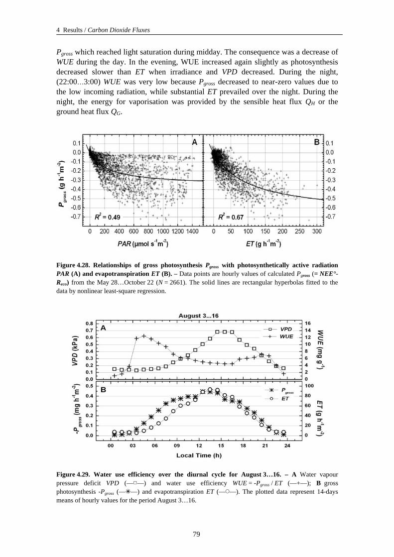
4 Results / Carbon Dioxide Fluxes
Pgross which reached light saturation during midday. The consequence was a decrease of WUE during the day. In the evening, WUE increased again slightly as photosynthesis decreased slower than ET when irradiance and VPD decreased. During the night, (22:00…3:00) WUE was very low because Pgross decreased to near-zero values due to the low incoming radiation, while substantial ET prevailed over the night. During the night, the energy for vaporisation was provided by the sensible heat flux QH or the ground heat flux QG.
Figure 4.28. Relationships of gross photosynthesis Pgross with photosynthetically active radiation PAR (A) and evapotranspiration ET (B). – Data points are hourly values of calculated Pgross (= NEE°-Reco) from the May 28…October 22 (N = 2661). The solid lines are rectangular hyperbolas fitted to the data by nonlinear least-square regression.
Figure 4.29. Water use efficiency over the diurnal cycle for August 3…16. – A Water vapour pressure deficit VPD (—□—) and water use efficiency WUE = -Pgross / ET (—+—); B gross photosynthesis -Pgross (—✴—) and evapotranspiration ET (—◯—). The plotted data represent 14-days means of hourly values for the period August 3…16.
79
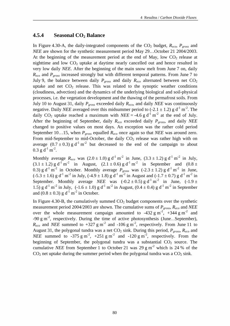
4 Resultss / Carbon Dioxide Fluxes
4.5.4 Seasonal CO2 Balance
In Figure 4.30-A, the daily-integrated components of the CO2 budget, Reco, Pgross and NEE are shown for the synthetic measurement period May 29…October 21 2004/2003. At the beginning of the measurement period at the end of May, low CO2 release at nighttime and low CO2 uptake at daytime nearly cancelled out and hence resulted in very low daily NEE. After the beginning of the main snow melt from June 7 on, daily Reco and Pgross increased strongly but with different temporal patterns. From June 7 to July 9, the balance between daily Pgross and daily Reco alternated between net CO2 uptake and net CO2 release. This was related to the synoptic weather conditions (cloudiness, advection) and the dynamics of the underlying biological and soil-physical processes, i.e. the vegetation development and the thawing of the permafrost soils. From July 10 to August 31, daily Pgross exceeded daily Reco, and daily NEE was continuously negative. Daily NEE averaged over this midsummer period to (-2.1 ± 1.2) g d-1 m-2. The daily CO2 uptake reached a maximum with NEE = -4.6 g d-1 m-2 at the end of July. After the beginning of September, daily Reco exceeded daily Pgross, and daily NEE changed to positive values on most days. An exception was the rather cold period September 10…15, when Pgross equalled Reco once again so that NEE was around zero. From mid-September to mid-October, the daily CO2 release was rather high with on average (0.7 ± 0.3) g d-1 m-2 but decreased to the end of the campaign to about 0.3 g d-1 m-2.
Monthly average Reco was (2.0 ± 1.0) g d-1 m-2 in June, (3.3 ± 1.2) g d-1 m-2 in July, (3.1 ± 1.2) g d-1 m-2 in August, (2.1 ± 0.6) g d-1 m-2 in September and (0.8 ± 0.3) g d-1 m-2 in October. Monthly average Pgross was (-2.3 ± 1.2) g d-1 m-2 in June, (-5.3 ± 1.6) g d-1 m-2 in July, (-4.9 ± 1.8) g d-1 m-2 in August and (-1.7 ± 0.7) g d-1 m-2 in September. Monthly average NEE was (-0.2 ± 0.5) g d-1 m-2 in June, (-1.9 ± 1.5) g d-1 m-2 in July, (-1.6 ± 1.0) g d-1 m-2 in August, (0.4 ± 0.4) g d-1 m-2 in September and (0.8 ± 0.3) g d-1 m-2 in October.
In Figure 4.30-B, the cumulatively summed CO2 budget components over the synthetic measurement period 2004/2003 are shown. The cumulative sums of Pgross, Reco and NEE over the whole measurement campaign amounted to -432 g m-2, +344 g m-2 and -90 g m-2, respectively. During the time of active photosynthesis (June…September), Reco and NEE summed to +327 g m-2 and -106 g m-2, respectively. From June 11 to August 31, the polygonal tundra was a net CO2 sink. During this period, Pgross, Reco and NEE summed to -375 g m-2, +251 g m-2 and -120 g m-2, respectively. From the beginning of September, the polygonal tundra was a substantial CO2 source. The cumulative NEE from September 1 to October 21 was 29 g m-2 which is 24 % of the CO2 net uptake during the summer period when the polygonal tundra was a CO2 sink.
80
4 Results / Carbon Dioxide Fluxes
Figure 4.30. CO2 budget components during summer and autumn: NEE, Reco and Pgross. – A Daily integrated CO2 budget components; B Cumulative curves of CO2 budget components over the investigation period. NEE (black) was measured by the eddy covariance system. Reco (stripes) and Pgross (grey) were estimated by empirical models (Chapter 3.4.3). The data are not stacked but NEE is overlaid on Reco and Pgross. Data were arranged so that they follow the seasonal course. Note that the data were recorded in two separate years and that the 2004 data are displayed before the 2003 data! The dotted lines indicate the period when the polygonal tundra represented a net CO2 sink.
81
4 Resultss / Carbon Dioxide Fluxes
4.5.5 Estimated Annual CO2 Budget
The annual CO2 budget was assessed by combining the NEE measurements of the measurement campaigns 2003 (May 29…July 19) and 2004 (July 20…October 21) with estimated values of Reco for the winter and spring period October 22…May 28 (about 7½ months). The empirical exponential models that described the control of Reco by surface or air temperature during the measurement periods (Figure 4.25) were found to be not appropriate for modelling of the wintertime Reco. Also the widely used function of Lloyd and Taylor [1994] for modelling Reco with soil temperature as the main driving force was not applicable for this purpose. It was considered that all fitted functions which relate Reco to temperature for the summer and the autumnal period of refreezing could not be transferred to the periods when soils were completely frozen during winter and spring because the temperature response of Reco was strongly dependent on the thickness of the unfrozen soil layer during the respective season.
This study followed a rather simple but conservative approach for estimating Reco during winter and spring. The period for which Reco had to be modelled was divided in two periods which were expected to behave differently in terms of Reco (Figure 4.31). The two periods were separated by the date when the soils of the polygonal tundra were completely frozen. This point of time, derived from the soil temperature measurements of the soil survey station, was found to be on November 17, 2003 (point C in Figure 4.31). During the second period, November 17…May 28, Reco was set constant to the Reco value observed during the night between May 28 and May 29 (point D in Figure 4.31), when the soils were still completely frozen (Chapter 4.1.3, Figure 4.3) and the minimum nightly Reco of the measurement period was measured (0.003 g h-1 m-2). This value falls at the lower end of the range of mean winter CO2 fluxes at similar tundra sites reported by other authors [Fahnestock et al., 1998; Oechel et al., 1997; Panikov and Dedysh, 2000; Zimov et al., 1993; Table 5.1]. During the first period October 22…November 17, Reco was estimated by linear interpolation between the measured Reco at October 21 (0.013 g h-1 m-2; point B in Figure 4.31) and the estimated Reco value for the second period (0.003 g h-1 m-2) on November 17 (point C).
In Figure 4.31, the estimated annual CO2 budget is presented. The cumulative NEE was -58 g m-2 during the measurement campaign 2003 (point A to point B; 94 days) and -32 g m-2 during the measurement campaign 2004 (point D to point E; 53 days). The cumulative estimated NEE during the first modelling period, when the soils were not completely frozen (point B to point C; 26 days), amounted to +5 g h-1 m-2. The cumulative estimated NEE during the second modelling period, when the soils were completely frozen (point C to point D; 194 days), amounted to +14 g m-2. The cumulative estimated NEE from October to May was +35 g m-2. The cumulative combined NEE for the whole year from July 20, 2003 to July 19 2004, was -71 g m-2. Thus, the polygonal tundra of the Lena River Delta was assessed to be a sink of CO2 during the investigation period. Approximately 432 gram CO2 per square-meter was assimilated by the vegetation over the year while about 363 gram CO2 per square meter was respired by the plants and the soil organisms, which is about 84 % of the annual CO2 assimilation by the vegetation.
82
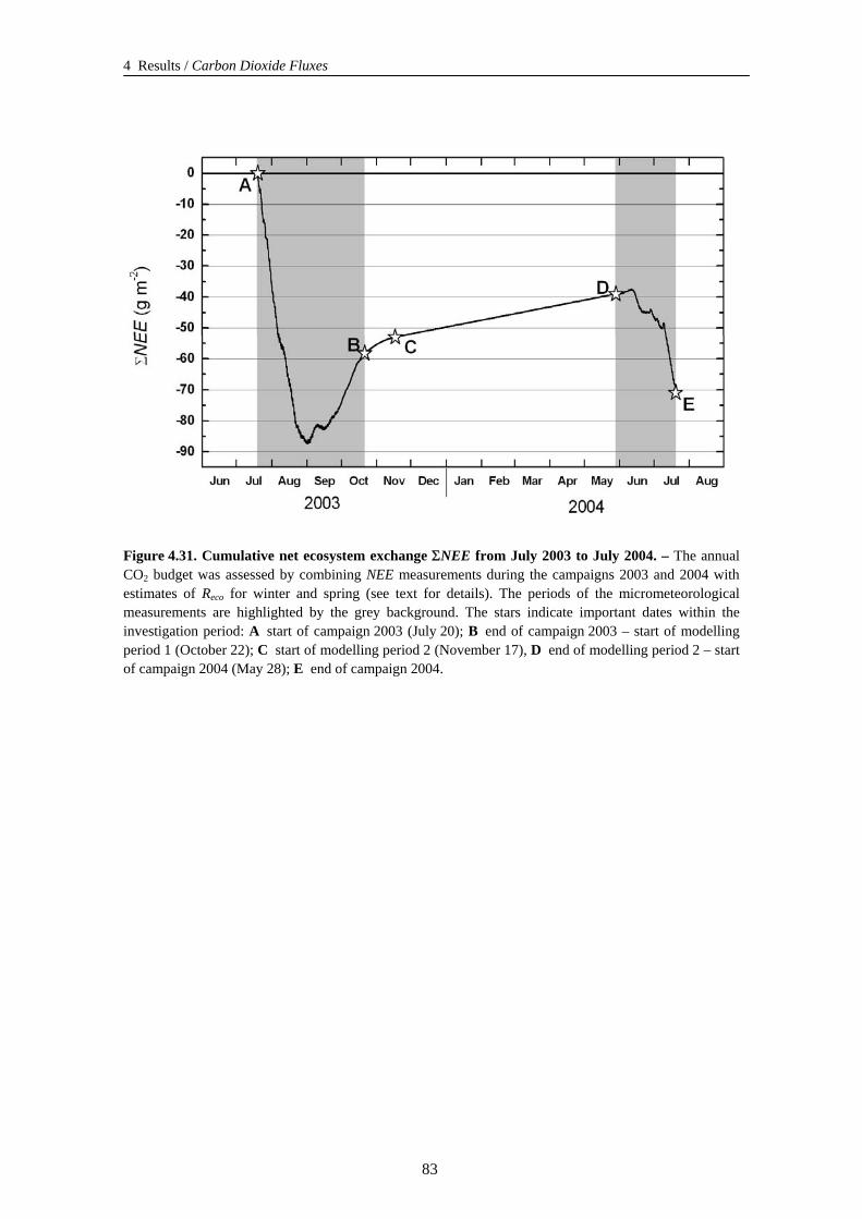
4 Results / Carbon Dioxide Fluxes
Figure 4.31. Cumulative net ecosystem exchange ΣNEE from July 2003 to July 2004. – The annual CO2 budget was assessed by combining NEE measurements during the campaigns 2003 and 2004 with estimates of Reco for winter and spring (see text for details). The periods of the micrometeorological measurements are highlighted by the grey background. The stars indicate important dates within the investigation period: A start of campaign 2003 (July 20); B end of campaign 2003 – start of modelling period 1 (October 22); C start of modelling period 2 (November 17), D end of modelling period 2 – start of campaign 2004 (May 28); E end of campaign 2004.
83
5 Discussion / The Energy and Water Balance at Wet Arctic Tundra
5 Discussion
5.1 The Energy and Water Balance at Wet Arctic Tundra
The energy exchange between land, sea, ice and the atmosphere drives the Earth’s climate on local, regional and, ultimately, global scales [Eugster et al., 2000]. A thorough understanding of the energy exchange processes at the arctic surfaces is a prerequisite for assessing the impacts of climatic change on the arctic ecosystems and the possible feedbacks on the climate system. However, only little information is available on the energy balance of the extensive Siberian Arctic [Balobaev, 1997; Boike et al., 1998, 2003a; Kodama et al., 2000; Friedrich, 2001], where the climate differs considerably from that of the European or North-American Arctic. The Siberian Arctic is characterised by more continental conditions with larger annual temperature amplitudes, less precipitation, less snow cover and deeper and colder permafrost. The here presented micrometeorological results demonstrate the major characteristics of the surface energy balance of wet arctic tundra in the Lena River Delta.
Radiation
The annual average of -Qs* at the Lena Delta amounted to 11 W m-2 (July 20, 2003 to July 19, 2004), which is at the low end of the -Qs* range of 13 W m-2…25 W m-2
reported for tundra surfaces [Bramer, 1982]. For comparison, typical annual averages of -Qs* are about 50 W m-2 in the temperate regions and 100 W m-2 in the tropics [Briggs and Smithson, 1994]. The energy fluxes in the Lena River Delta showed the strong seasonality which is typical for the Arctic [Ohmura, 1982b]. -Qs* was a heat source between the middle of April to the end of September and was an energy sink for the rest of the year. It should be noted that polar day does not imply the lack of diurnal change. On the contrary, the energy fluxes showed marked diurnal variations during summer, which had a major impact on the over-all energy balance in addition to the overriding seasonality.
The cumulative sum of -Qs* over summer was rather low during our campaigns compared to values reported for the North-American or European Arctic. During summer, -Qs* summed to only 607 MJ m-2, which is equivalent to 18 % of the extraterrestrial solar radiation (ETSR) to a horizontal surface in the same period. Ohmura [1982b] reported that -Qs* summed over the summer was 854 MJ m-2 (26 % of ETSR) at Barrow, Alaska (71°11'N, 156°40'W) and to 699 MJ m-2 (20 % of ETSR) at Axel Heiberg Island, North-West-Territories, Canada (79°21'N, 90°30'W). Lloyd et al. [2001] published cumulative values of -Qs* summed over June 9…August 29 of 700 W m-2…800 MJ m-2 for Zackenberg, North East Greenland (74°28'N, 20°34'W), Skalluvaara, Finland (69°49'N, 27°12'E) and Kaamanen, Finland (69°08'N, 27°17'E). Only at Ny-Ålesund, Svalbard (78°56'N, 11°55'E), the latter authors measured similarly low -Qs* as observed in this study. The low cumulative summer -Qs* measured in the
84
5 Discussion / The Energy and Water Balance at Wet Arctic Tundra
Lena River Delta can be explained by three main causes: (1.) the long duration of the snow cover towards the solstice until June 17, (2.) the frequent occurrence of overcast sky in summer as reflected by a low cumulative global radiation during summer of 1455 MJ m-2. (42 % of ETSR compared to 48 % of ETSR at Barrow [Ohmura, 1982], and (3.) frequent events of warm air advection from the Siberian hinterland. The third point is probably the most important for the big differences in -Qs* between the Lena River Delta and the other Arctic sites, respectively. Compared to the conditions reported by Ohmura [1982b] for Barrow, the surface absorbed less solar radiation over the summer (1049 MJ m-2 versus 1113 MJ m-2) but emitted significantly more long-wave radiation (2772 MJ m-2 versus 2612 MJ m-2). More long-wave radiation implies higher surface temperatures which are very likely to be caused by substantial energy fluxes from advective warm air masses to the surface via QH.
Ground heat flux QG
A large fraction, more than one fourth, of -Qs* gained by the surface during summer was partitioned into QG. (27 %, polygon rim 29 %, polygon centre 25 %). Similar percentages were reported by Boike et al. [1998] for a permafrost site on the Taymyr Peninsula, Siberia (24 %), and by Friedrich [2001] for the polygonal tundra of the Lena River Delta (30 %). Actually, the soil-meteorological sensors used by the latter author in the summers 1998 and 1999 were installed within only 50 m from the sensors used in this study [Wille et al., 2003]. It is noteworthy that both this study and the study of Friedrich, which were independent projects with differing equipment, set-up and calculation methods (Friedrich: soil temperature gradient method), found QG values of the same, rather high order of magnitude (about 30 % of -Qs*). The higher QG observed by Friedrich was probably caused by on average lower soil moisture at his sites. His sites resembled the polygon rim site of this study; no measurements at the centre of a wet polygon were performed. An even higher QG /-Qs* fraction (more than 40 %) was reported for an upland tundra site near to Tiksi, Northern Siberia [Kodama et al., 2000].
On the other hand, the fraction of -Qs* partitioned into QG appears to be significantly lower in the North-American and European Arctic compared to the observations of this study. It was 14 % at an upland tundra site on Axel Heiberg Island, Canada [Ohmura, 1982b], 15 % at a moist to wet polygonal tundra at the arctic coastal plain of the North Slope of Alaska [Vourlites and Oechel, 1997], 10 %…15 % at an high-arctic semidesert on Svalbard [Harding and Lloyd, 1998], around 10 % at wet sedge tundra and 16 % at tussock tundra on the North Slope of Alaska [Harazono et al., 1998], and 11 % at an Arctic fen (wet sedge tundra) at North-East Greenland [Soegaard et al., 2001]. Also in the most comprehensive review of Arctic energy balance studies by Eugster et al. [2000], almost all reported QG /-Qs* fractions for tundra surfaces ranged between 10 % and 20 %. However, no data from Siberian tundra sites were included in this review.
The QG data of the circumpolar region compiled here highlight the importance of the special permafrost conditions for the energy balance of the Siberian arctic tundra. The permafrost in the Lena River Delta region belongs to the coldest permafrost on earth with mean temperatures of -11 °C…-13°C [Kotlyakov and Khromova, 2002; NSIDC, 2003]. In North-America, such low permafrost temperatures are only encountered in the semideserts of the Canadian Arctic Archipelago [Natural Resources Canada, 1995].
85
5 Discussion / The Energy and Water Balance at Wet Arctic Tundra
The low permafrost temperatures lead to steep temperature gradients in the permafrost soils promoting high QG in spring and summer [Boike et al., 2003b], when the ground surface temperature can rise up to 30 °C. Furthermore, the permafrost soils and sediments of the North-Siberian lowlands are characterised by high water/ice content. The high water content permits the wet permafrost soils to absorb large energy quantities since (1.) the heat capacity and heat conductivity of water and ice are high and (2.) much energy is needed for the phase change between ice and liquid water. For the summer period of active-layer melting, it can be presumed that the predominant fraction of QG was consumed by melting of the ice. Boike et al. [1998] calculated for a permafrost soil on the Taymyr Peninsula, which had a volumetric water content of 30 %…40 %, that 70 %…100 % of QG went into the phase change of water during the thawing period.
Summer heat uptake and winter heat loss of soils were larger at the polygon rim than in the centre which is explained by differences in soil heat conductivity. The heat conductivity of the top 5 cm of the Typic Aquiturbel at the rim, which was moist and had a moderate organic matter content, was modelled to be on average 0.7 W m-1 K-1 in summer and 1.43 W m-1 K-1 in winter (model of de Vries [1963]). The modelled heat conductivity of the top 5 cm of the wet and organic-rich Typic Historthel in the centre was 0.56 W m-1 K-1 during summer and 2.07 W m-1 K-1 during winter. Thus, the higher heat conductivity of the Typic Aquiturbel led to larger heat uptake in summer. During winter, the heat conductivity of the Typic Historthel was higher, but nevertheless the heat loss was smaller than at the rim due to less stored heat and the much higher insulating snow-pack compared to the rim.
Sensible and latent heat fluxes QE, QH
As a consequence of the rather low -Qs* and the large QG, the available energy (-Qs* -QG) that could be partitioned into the turbulent atmospheric fluxes QH and QE was limited. Particularly, QH was forced to low daily and seasonal averages in summer by the heat sink effect of the permafrost soils, which cooled the ground surface and thus restrained QH from the surface to the atmosphere. Only 26 % of the summer surplus of -Qs* was partitioned into QH. The reason for this lies more in the diurnal and seasonal pattern of QH than in its amplitude: Indeed, QH frequently equalled or exceeded QG and QE when -Qs* was large, around midday and during midsummer (β up to 1.6). However, it rose late to positive values and dropped early to negative values in the diurnal cycle and in the course of the season, respectively. Thus, much of the energy transferred from the surface to the atmosphere was in effect returned to the surface during night or winter, respectively.
The main energy sink was QE which consumed 41 % of -Qs* calculated over the summer. Thus, the polygonal tundra behaved during the summers 2003 and 2004 like a typical wetland in terms of energy partitioning between QH and QE (mean Bowen ratio: 0.63). By contrast, Friedrich [2001] reported almost reversed proportions of QH (44 %) and QE (25 %) for the same tundra type during the summer 1999 (mean Bowen ratio: 1.76). This discrepancy is probably due to different reasons: The summer precipitation was much lower in 1999 than in 2003 (55 mm versus 164 mm). In 1999, many polygon centres dried up which were normally inundated. Certainly, such dry conditions could
86
5 Discussion / The Energy and Water Balance at Wet Arctic Tundra
have reduced QE substantially. However, the study of Friedrich is considered here to have underestimated QE systematically due to several methodical problems: The fetch of wet polygonal tundra was insufficient for the applied Bowen ratio method [Schmid, 1997, Stannard, 1997; Horst, 1999] so that neighbouring areas with lower soil moisture were likely to influence the QE measurements considerably (see Figure 2.3). Furthermore, the air humidity gradients were corrected for sensor inaccuracies by a method that could significantly reduce the measured gradients and thus the calculated QE values. Therefore, it does not appear sensible to compare the QH and QE values from this study and the work of Friedrich for evaluating the interannual variability of the turbulent heat fluxes in relation to climatic fluctuations.
The relative proportions of QH and QE observed in this study during the summers 2003 and 2004 were similar to values reported for other arctic and subarctic wetlands. The fractions of -Qs* partitioned into QH and QE during summer were 25 % versus 63 % at a subarctic fen in Quebec, Canada [Moore et al., 1994], 29% versus 57 % at a flooded sedge tundra at the North Slope of Alaska [Harazono et al., 1998], 27 % versus 39 % at an Arctic fen at North-East Greenland [Soegaard et al., 2001], 28 % versus 64 % at two wetland tundra sites in the Canadian Subarctic [Eaton et al., 2001], and 34 % versus 51 % at a subarctic elevated mire in Northern Finland [Lloyd et al., 2001]. At moist tussock tundra and arctic semideserts, QH has normally greater importance as sink in the energy balance with up to 42 % of -Qs* [Fitzjarrald and Moore, 1992; Harding and Lloyd, 1998; McFadden et al., 1998; Vourlites and Oechel, 1999; Eugster et al., 1997, 2000; Kodama et al., 2000; Eaton et al., 2001].
A decrease of the Bowen ratio over the summer season was observed in this study although the water level was dropping simultaneously. Daily values of QH and QE were of the same magnitude during the first half of the summer while daily QE clearly exceeded QH in the second half. This relative increase of QE over the summer was also reported for several other wetlands of the European Arctic and Greenland [Lloyd et al, 2001] and can be explained by the phenology of the vegetation. After the vegetation had emerged from the snow pack, it took time until the greening reached its maximum. Since the transpiration by vascular plants is closely related to their photosynthetic activity, QE gained higher importance in the second half of the summer when the vegetation was already fully developed. By contrast, Vourlites and Oechel [1997] reported a decrease of the Bowen ratio over the summer for a moist to wet polygonal tundra indicating increasing water stress of the vegetation with a dropping water table.
Influence of advection on the energy fluxes
Harazono et al. [1998] found no clear trend of the Bowen ratio related to the vegetation development over summer at wet sedge tundra at the North Slope of Alaska and related the fluctuations of the Bowen ratio to air temperature variations connected to synoptical weather patterns. The latter authors noted that the synoptical weather patterns, namely either onshore winds from the Arctic Ocean or offshore winds from the continental hinterland, can be of major importance for the energy balance of the arctic tundra. This finding is also valid for the investigation area of this study: During periods of advection of warm and dry air masses from the Siberian hinterland, QH is low or even negative for most of the day while substantial QE is taking place due to high VPD. Thus, low or
87
5 Discussion / The Energy and Water Balance at Wet Arctic Tundra
negative Bowen ratios were observed. During periods of advection of cold air from the Arctic Ocean, QH and likewise the Bowen ratio can be rather high at least around midday. Since the advection of air masses strongly affects the energy partition at the surface, the prevailing large-scale atmospheric circulation patterns, for example the phase of the Arctic Oscillation [Dorn et al., 2000; Thompson and Wallace, 2001; Ostermeier and Wallace, 2003], have a strong influence on the function of tundra as heat sink or source.
Importance of the snow pack for the annual energy budget
The annual energy balance of the arctic tundra of the Lena River Delta was strongly influenced by the effects of the snow pack, which covered the tundra surface for eight months during the investigation period (July 20, 2003 to July 19, 2004). Due to the high albedo of snow, -Qs* was nearly five times smaller before than after snow melt. Thus, the timing of snow melt in early summer has a major influence on the annual -Qs* surplus. Approximately 5 % of the summer surplus of -Qs* was consumed by the snow melt. The snow cover is very heterogeneous at the polygonal tundra of the Lena Delta due to the prominent microrelief and pronounced snow drift caused by frequent strong winds [Boike et al, 2003b]. Due to this high spatial variability of the snow cover, also the thermal conditions in the permafrost soils and the energy fluxes vary substantially within few meters. During winter, a thick snow pack of 40 cm…50 cm depth insulated effectively the ground in the polygon centres thus damping heat losses of the ground via QG. By contrast, the snow cover on the elevated polygon rims was thin or even absent, leading to strong cooling in winter. Another important effect of snow on the energy balance is the alteration of the surface aerodynamic characteristics: The surface roughness length was 100 times smaller when the tundra was covered with snow leading to reduced turbulent heat transfer between the ground and the atmosphere.
The water balance
Precipitation was very high in the period of consideration, from July 20, 2003 to July 19, 2004. Unfortunately, no continuous precipitation records are available for Samoylov Island. Therefore, precipitation data from the Russian meteorological station Stolb, which is situated 20 km east of Samoylov Island, were used for interannual comparison (available data from March 2000 to June 2004) [HMCR, 2004]. However, it has to be noted that the summer precipitation values determined by the automatic weather station (AMLS) at Samoylov Island during the micrometeorological campaigns were considerably larger (about 20 %…30 %) than the respective values recorded at Stolb. It is not clear if this mismatch reflects real small-scale spatial variability of rainfall [Krajewski et al., 1998; Jensen and Pedersen, 2005] or is due to methodical problems of either the AMLS at Samoylov Island or of the station Stolb [Yang et al., 2001; Lanza and Stagi, 2002]. The total annual precipitation measured at Stolb from July 20, 2003 to July 19, 2004 (~311 mm a-1) exceeded the average annual precipitation of the two preceding years 2001 and 2002 ((202 ± 18) mm a-1) by about 50 %. A big part of the total precipitation took place during high-intensity rain events. More than a fifth of the annual precipitation fell during one week of heavy rain at the end of July
88
5 Discussion / The Energy and Water Balance at Wet Arctic Tundra
2003. 10 % fell during two days at the beginning of July 2004. Another 10 % fell during a strong snow storm at the beginning of December (seven days).
Due to the large amount of snowfall in the winter 2003/2004 (140 mm), the snow pack was high and consequently the amount of water set free during snow melt was large (70 mm…100 mm). A substantial portion of the accumulated snow was lost to the atmosphere through sublimation. By comparing the snowfall measurements at Stolb and the measurements of snow height and snow density at Samoylov Island by Wille and Boike [2006], the magnitude of sublimation during the cold season was estimated to 30 %…50 % of the total snowfall amount. This high value is reasonable considering the high wind speed at Samoylov Island and the prominent snow drift patterns observed at the site [Boike et al., 2003]. Snow grains which are saltating or in suspension during wind transport suffer rapid rates of sublimation [Sturm et al., 2001]. The mean wind speed from October 2003 to May 2004 was (3.9 ± 2.8) m s-1 with strong winds of up to 14 m s-1 occurring frequently. The high sublimation estimate is consistent with findings of Liston and Sturm [2002], who noted that up to 40 % of the winter snow accumulation can be removed by sublimation at windy, open places.
Despite the large input of water as rainfall or snow melt water, the summer evapotranspiration was rather low compared to similar sites in the Arctic. Daily ET averaged to only (1.1 ± 0.7) mm d-1 over the summer, which is 94 % of ET 7 at an Arctic fen in North-East Greenland [Soegaard et al., 2001], 81 %…91 % of ET at two moist to wet polygonal tundra sites at the arctic coastal plain of the North Slope of Alaska [Vourlites and Oechel, 1997] and 52 % of ET at wet sedge tundra at the North Slope of Alaska [Harazono et al., 1998]. Mean daily ET measured in this study was also lower than ET reported for many tussock and upland tundra sites. It was only 93 % of ET at a high-arctic semidesert on Svalbard [Harding and Lloyd, 1998], 66 %…92 % of ET at moist tussock tundra at the North Slope of Alaska depending on the investigation year [Vourlites and Oechel, 1999], 84 % at dry tussock tundra at the North Slope of Alaska [Harazono et al., 1998] and 77 % of ET at upland tundra at Axel Heiberg Island, North-West-Territories, Canada [Ohmura, 1982b].
The analysis of the aerodynamic resistance ra, the surface resistance rs and the decoupling factor Ω showed that the limitation of ET was mainly caused by the low available energy as discussed above and only little by the interactions between vegetation and atmosphere. The observed midday ra, which is a function of wind speed and surface roughness length, fell in the range reported for moist and wet tundra ecosystems in Alaska. On the other hand, midday rs was on average significantly lower in the Lena River Delta (median 121 s m-1) compared with tundra sites in Alaska although these sites were characterised by higher ET [Fitzjarrald and Moore, 1992; McFadden et al., 1998, 2003]. At sites with similar low rs as in the Lena River Delta, ET was twice as high as observed in this study [Harazono et al., 1998]. Thus, rather low rs did not lead to high ET at the polygonal tundra of the Lena River Delta.
7 Since all authors reported ET for different time spans, it is most instructive to compare ET at the different sites by relative values, which were calculated by comparing ET observed in this study with the ET reported by other authors for the same time period as noted in the respective publication.
89
5 Discussion / The Energy and Water Balance at Wet Arctic Tundra
Stomatal closure was not observed during the measurement period. Carex aquatilis, the dominating vascular plant species at the site, is known to be rather insensitive to increasing VPD [Miller et al., 1980]. However, the surface conductance rs increased moderately with increasing surface-to-air water vapour pressure deficit VPDs-a, which is explained by the response of the moss layer to limited water availability. It is considered that a substantial part (50 %…85 %) of ET is evaporation from the moss layer [Vourlites and Oechel, 1999; Miller et al., 1980; Grant et al., 2003]. Although mosses lack stomatal control, their resistance to water loss increases exponentially as tissue water decreases [Oechel and Sveinbjörnsson, 1978, cited in Vourlites and Oechel, 1999; McFadden et al., 2003].
The observed values of Ω was on average significantly higher compared to values reported by McFadden et al. [1998, 2003] for different tundra types in Alaska demonstrating a relatively weak coupling between vegetation and atmosphere at the Lena River Delta and a low impact of rs and VPD on ET. Only during very pronounced advection of warm and dry air from the South, rs increased and Ω decreased significantly showing a stronger effect of rs and VPD on the limitation of ET during these periods. A similar relationship between the vegetation-atmosphere coupling and the advective conditions were reported by Harazono et al. [1998] for wet sedge tundra in Alaska.
The high precipitation combined with relative low evapotranspiration led to substantial run-off from the polygonal tundra. The run-off was estimated to amount to 170 mm a-1… 210 mm a-1 from July 2003 to July 2004. On the other hand, the soil water storage did not increase but rather decreased slightly over the measurement period. This surprising fact can be explained as follows: Heavy summer precipitation events initially raise the water level in the waterlogged permafrost soils of the polygon centres. If the water level greatly exceeds the normal water table position, the water finds more easily ways across the polygon rims that otherwise dam the standing water in the polygon centres. When water starts to flow, thermoerosion8 rapidly deepens the outflow, and deep gullies can form leading to pronounced drainage. Thus, a strongly increased summer precipitation promotes paradoxically not wet soil conditions but desiccation of wet polygonal tundra in the long term. In summer 2003, these thermoerosion processes initiated by heavy rainfall were very pronounced at the polygonal tundra, even at the centre of Samoylov Island (Figure 5.1), thus imparting an impression of what could happen to permafrost landscapes when precipitation will rise further in the future as predicted by climate models. Consistent with these observations, Smith et al. [2005] reported a decline in the number and size of lakes in Arctic Siberia despite slightly increased precipitation, which is probably also caused by enhanced drainage due to degradation of permafrost.
Summarizing, the surface energy balance of wet polygonal tundra in the Lena River Delta was determined mainly by (1.) the polar and distinctly continental climate, (2.) the very cold and ice-rich permafrost which underlies the tundra in Northern Siberia, (3.) the wetland character of polygonal tundra, (4.) the position at the interface between the
8 The term thermoerosion refers to erosion by water combined with its thermal effect on frozen ground [Washburn, 1979; French, 1996]
90
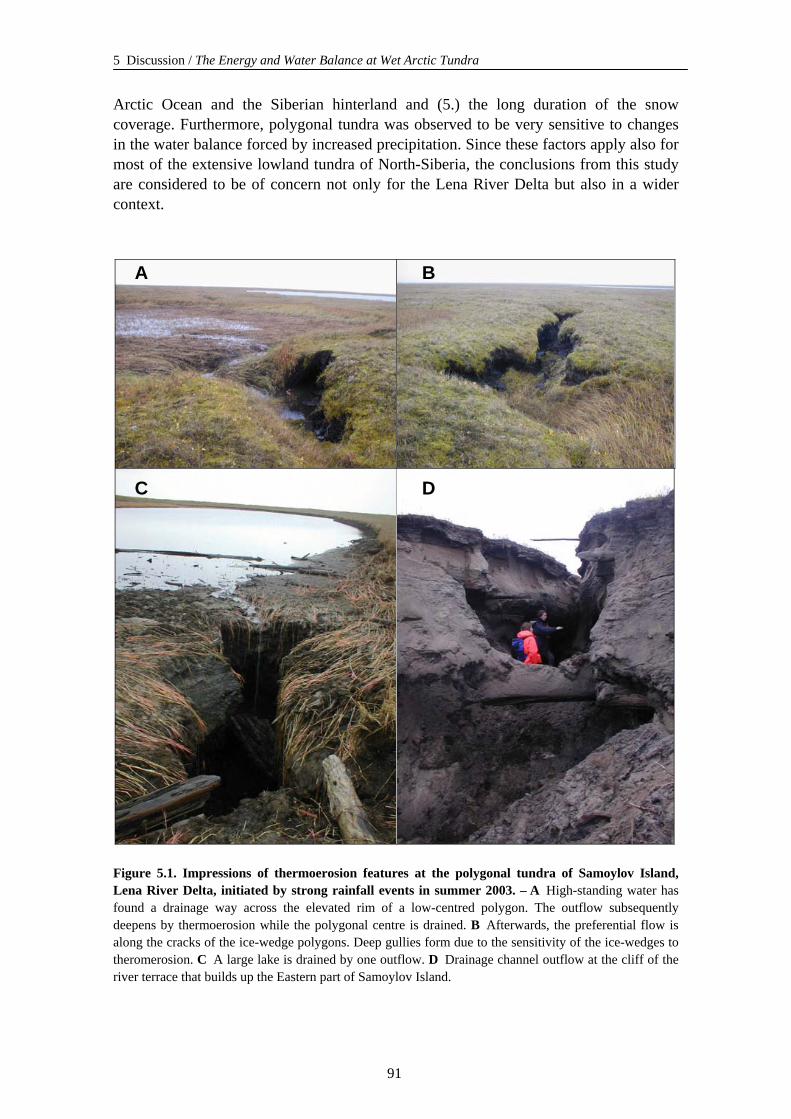
5 Discussion / The Energy and Water Balance at Wet Arctic Tundra
Arctic Ocean and the Siberian hinterland and (5.) the long duration of the snow coverage. Furthermore, polygonal tundra was observed to be very sensitive to changes in the water balance forced by increased precipitation. Since these factors apply also for most of the extensive lowland tundra of North-Siberia, the conclusions from this study are considered to be of concern not only for the Lena River Delta but also in a wider context.
D C
B A
Figure 5.1. Impressions of thermoerosion features at the polygonal tundra of Samoylov Island, Lena River Delta, initiated by strong rainfall events in summer 2003. – A High-standing water has found a drainage way across the elevated rim of a low-centred polygon. The outflow subsequently deepens by thermoerosion while the polygonal centre is drained. B Afterwards, the preferential flow is along the cracks of the ice-wedge polygons. Deep gullies form due to the sensitivity of the ice-wedges to theromerosion. C A large lake is drained by one outflow. D Drainage channel outflow at the cliff of the river terrace that builds up the Eastern part of Samoylov Island.
91
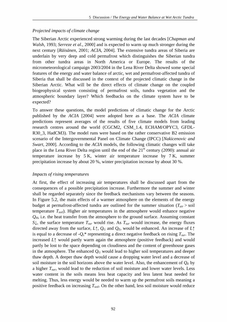
5 Discussion / The Energy and Water Balance at Wet Arctic Tundra
Projected impacts of climate change
The Siberian Arctic experienced strong warming during the last decades [Chapman and Walsh, 1993; Serreze et al., 2000] and is expected to warm up much stronger during the next century [Räisänen, 2001; ACIA, 2004]. The extensive tundra areas of Siberia are underlain by very deep and cold permafrost which distinguishes the Siberian tundra from other tundra areas in North America or Europe. The results of the micrometeorological campaign 2003/2004 in the Lena River Delta showed some special features of the energy and water balance of arctic, wet and permafrost-affected tundra of Siberia that shall be discussed in the context of the projected climatic change in the Siberian Arctic. What will be the direct effects of climate change on the coupled biogeophysical system consisting of permafrost soils, tundra vegetation and the atmospheric boundary layer? Which feedbacks on the climate system have to be expected?
To answer these questions, the model predictions of climatic change for the Arctic published by the ACIA [2004] were adopted here as a base. The ACIA climate predictions represent averages of the results of five climate models from leading research centres around the world (CGCM2, CSM_1.4, ECHAM/OPYC3, GFDL-R30_3, HadCM3). The model runs were based on the rather conservative B2 emission scenario of the Intergovernmental Panel on Climate Change (IPCC) [Nakicenovic and Swart, 2000]. According to the ACIA models, the following climatic changes will take place in the Lena River Delta region until the end of the 21st century (2090): annual air temperature increase by 5 K, winter air temperature increase by 7 K, summer precipitation increase by about 20 %, winter precipitation increase by about 30 %.
Impacts of rising temperatures
At first, the effect of increasing air temperatures shall be discussed apart from the consequences of a possible precipitation increase. Furthermore the summer and winter shall be regarded separately since the feedback mechanisms vary between the seasons. In Figure 5.2, the main effects of a warmer atmosphere on the elements of the energy budget at permafrost-affected tundra are outlined for the summer situation (Tair > soil temperature Tsoil). Higher air temperatures in the atmosphere would enhance negative QH, i.e. the heat transfer from the atmosphere to the ground surface. Assuming constant S↓, the surface temperature Tsur would rise. As Tsur would increase, the energy fluxes directed away from the surface, L↑, QG and QE, would be enhanced. An increase of L↑ is equal to a decrease of -Qs* representing a direct negative feedback on rising Tsur. The increased L↑ would partly warm again the atmosphere (positive feedback) and would partly be lost to the space depending on cloudiness and the content of greenhouse gases in the atmosphere. The enhanced QG would lead to higher soil temperatures and deeper thaw depth. A deeper thaw depth would cause a dropping water level and a decrease of soil moisture in the soil horizons above the water level. Also, the enhancement of QE by a higher Tsur, would lead to the reduction of soil moisture and lower water levels. Less water content in the soils means less heat capacity and less latent heat needed for melting. Thus, less energy would be needed to warm up the permafrost soils meaning a positive feedback on increasing Tsoil. On the other hand, less soil moisture would reduce
92
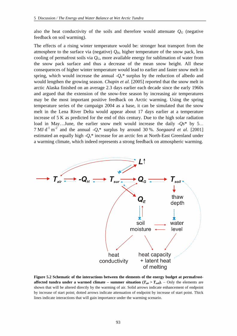
5 Discussion / The Energy and Water Balance at Wet Arctic Tundra
also the heat conductivity of the soils and therefore would attenuate QG (negative feedback on soil warming).
The effects of a rising winter temperature would be: stronger heat transport from the atmosphere to the surface via (negative) QH, higher temperature of the snow pack, less cooling of permafrost soils via QG, more available energy for sublimation of water from the snow pack surface and thus a decrease of the mean snow height. All these consequences of higher winter temperature would lead to earlier and faster snow melt in spring, which would increase the annual -Qs* surplus by the reduction of albedo and would lengthen the growing season. Chapin et al. [2005] reported that the snow melt in arctic Alaska finished on an average 2.3 days earlier each decade since the early 1960s and argued that the extension of the snow-free season by increasing air temperatures may be the most important positive feedback on Arctic warming. Using the spring temperature series of the campaign 2004 as a base, it can be simulated that the snow melt in the Lena River Delta would appear about 17 days earlier at a temperature increase of 5 K as predicted for the end of this century. Due to the high solar radiation load in May…June, the earlier snow melt would increase the daily -Qs* by 5… 7 MJ d-1 m-2 and the annual -Qs* surplus by around 30 %. Soegaard et al. [2001] estimated an equally high -Qs* increase for an arctic fen at North-East Greenland under a warming climate, which indeed represents a strong feedback on atmospheric warming.
Figure 5.2 Schematic of the interactions between the elements of the energy budget at permafrost-affected tundra under a warmed climate – summer situation (Tair > Tsoil). – Only the elements are shown that will be altered directly by the warming of air. Solid arrows indicate enhancement of endpoint by increase of start point; dotted arrows indicate attenuation of endpoint by increase of start point. Thick lines indicate interactions that will gain importance under the warming scenario.
93
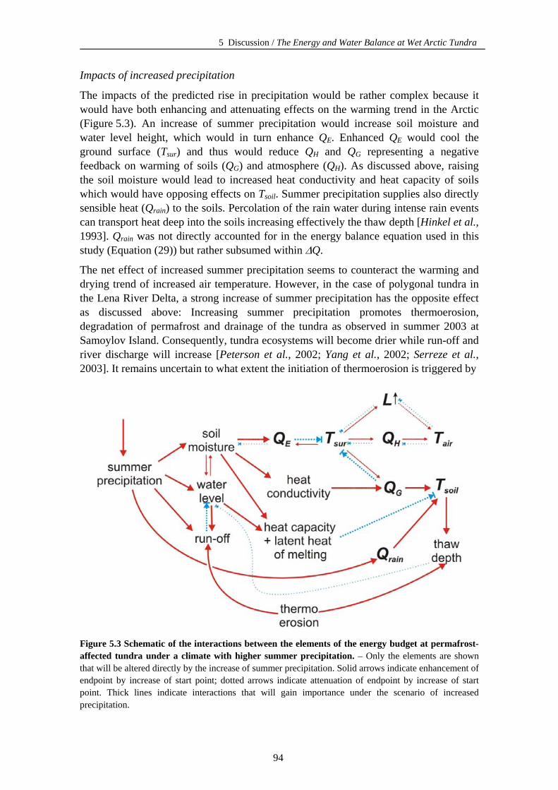
5 Discussion / The Energy and Water Balance at Wet Arctic Tundra
Impacts of increased precipitation
The impacts of the predicted rise in precipitation would be rather complex because it would have both enhancing and attenuating effects on the warming trend in the Arctic (Figure 5.3). An increase of summer precipitation would increase soil moisture and water level height, which would in turn enhance QE. Enhanced QE would cool the ground surface (Tsur) and thus would reduce QH and QG representing a negative feedback on warming of soils (QG) and atmosphere (QH). As discussed above, raising the soil moisture would lead to increased heat conductivity and heat capacity of soils which would have opposing effects on Tsoil. Summer precipitation supplies also directly sensible heat (Qrain) to the soils. Percolation of the rain water during intense rain events can transport heat deep into the soils increasing effectively the thaw depth [Hinkel et al., 1993]. Qrain was not directly accounted for in the energy balance equation used in this study (Equation (29)) but rather subsumed within ΔQ.
The net effect of increased summer precipitation seems to counteract the warming and drying trend of increased air temperature. However, in the case of polygonal tundra in the Lena River Delta, a strong increase of summer precipitation has the opposite effect as discussed above: Increasing summer precipitation promotes thermoerosion, degradation of permafrost and drainage of the tundra as observed in summer 2003 at Samoylov Island. Consequently, tundra ecosystems will become drier while run-off and river discharge will increase [Peterson et al., 2002; Yang et al., 2002; Serreze et al., 2003]. It remains uncertain to what extent the initiation of thermoerosion is triggered by
Figure 5.3 Schematic of the interactions between the elements of the energy budget at permafrost-affected tundra under a climate with higher summer precipitation. – Only the elements are shown that will be altered directly by the increase of summer precipitation. Solid arrows indicate enhancement of endpoint by increase of start point; dotted arrows indicate attenuation of endpoint by increase of start point. Thick lines indicate interactions that will gain importance under the scenario of increased precipitation.
94
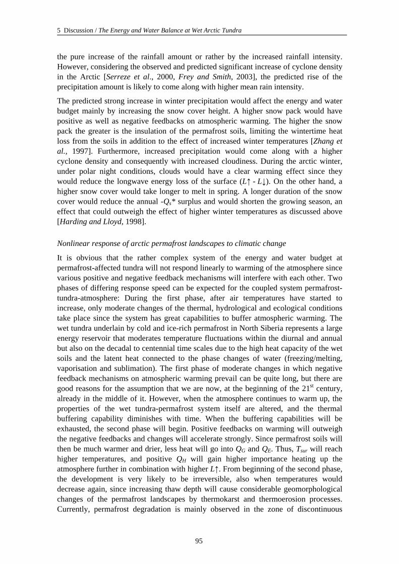
5 Discussion / The Energy and Water Balance at Wet Arctic Tundra
the pure increase of the rainfall amount or rather by the increased rainfall intensity. However, considering the observed and predicted significant increase of cyclone density in the Arctic [Serreze et al., 2000, Frey and Smith, 2003], the predicted rise of the precipitation amount is likely to come along with higher mean rain intensity.
The predicted strong increase in winter precipitation would affect the energy and water budget mainly by increasing the snow cover height. A higher snow pack would have positive as well as negative feedbacks on atmospheric warming. The higher the snow pack the greater is the insulation of the permafrost soils, limiting the wintertime heat loss from the soils in addition to the effect of increased winter temperatures [Zhang et al., 1997]. Furthermore, increased precipitation would come along with a higher cyclone density and consequently with increased cloudiness. During the arctic winter, under polar night conditions, clouds would have a clear warming effect since they would reduce the longwave energy loss of the surface (L↑ - L↓). On the other hand, a higher snow cover would take longer to melt in spring. A longer duration of the snow cover would reduce the annual -Qs* surplus and would shorten the growing season, an effect that could outweigh the effect of higher winter temperatures as discussed above [Harding and Lloyd, 1998].
Nonlinear response of arctic permafrost landscapes to climatic change
It is obvious that the rather complex system of the energy and water budget at permafrost-affected tundra will not respond linearly to warming of the atmosphere since various positive and negative feedback mechanisms will interfere with each other. Two phases of differing response speed can be expected for the coupled system permafrost-tundra-atmosphere: During the first phase, after air temperatures have started to increase, only moderate changes of the thermal, hydrological and ecological conditions take place since the system has great capabilities to buffer atmospheric warming. The wet tundra underlain by cold and ice-rich permafrost in North Siberia represents a large energy reservoir that moderates temperature fluctuations within the diurnal and annual but also on the decadal to centennial time scales due to the high heat capacity of the wet soils and the latent heat connected to the phase changes of water (freezing/melting, vaporisation and sublimation). The first phase of moderate changes in which negative feedback mechanisms on atmospheric warming prevail can be quite long, but there are good reasons for the assumption that we are now, at the beginning of the 21st century, already in the middle of it. However, when the atmosphere continues to warm up, the properties of the wet tundra-permafrost system itself are altered, and the thermal buffering capability diminishes with time. When the buffering capabilities will be exhausted, the second phase will begin. Positive feedbacks on warming will outweigh the negative feedbacks and changes will accelerate strongly. Since permafrost soils will then be much warmer and drier, less heat will go into QG and QE. Thus, Tsur will reach higher temperatures, and positive QH will gain higher importance heating up the atmosphere further in combination with higher L↑. From beginning of the second phase, the development is very likely to be irreversible, also when temperatures would decrease again, since increasing thaw depth will cause considerable geomorphological changes of the permafrost landscapes by thermokarst and thermoerosion processes. Currently, permafrost degradation is mainly observed in the zone of discontinuous
95
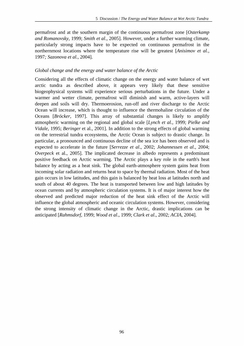
5 Discussion / The Energy and Water Balance at Wet Arctic Tundra
permafrost and at the southern margin of the continuous permafrost zone [Osterkamp and Romanovsky, 1999; Smith et al., 2005]. However, under a further warming climate, particularly strong impacts have to be expected on continuous permafrost in the northernmost locations where the temperature rise will be greatest [Anisimov et al., 1997; Sazonova et al., 2004].
Global change and the energy and water balance of the Arctic
Considering all the effects of climatic change on the energy and water balance of wet arctic tundra as described above, it appears very likely that these sensitive biogeophysical systems will experience serious perturbations in the future. Under a warmer and wetter climate, permafrost will diminish and warm, active-layers will deepen and soils will dry. Thermoerosion, run-off and river discharge to the Arctic Ocean will increase, which is thought to influence the thermohaline circulation of the Oceans [Bröcker, 1997]. This array of substantial changes is likely to amplify atmospheric warming on the regional and global scale [Lynch et al., 1999; Pielke and Vidale, 1995; Beringer et al., 2001]. In addition to the strong effects of global warming on the terrestrial tundra ecosystems, the Arctic Ocean is subject to drastic change. In particular, a pronounced and continuous decline of the sea ice has been observed and is expected to accelerate in the future [Serrezze et al., 2002; Johannessen et al., 2004; Overpeck et al., 2005]. The implicated decrease in albedo represents a predominant positive feedback on Arctic warming. The Arctic plays a key role in the earth's heat balance by acting as a heat sink. The global earth-atmosphere system gains heat from incoming solar radiation and returns heat to space by thermal radiation. Most of the heat gain occurs in low latitudes, and this gain is balanced by heat loss at latitudes north and south of about 40 degrees. The heat is transported between low and high latitudes by ocean currents and by atmospheric circulation systems. It is of major interest how the observed and predicted major reduction of the heat sink effect of the Arctic will influence the global atmospheric and oceanic circulation systems. However, considering the strong intensity of climatic change in the Arctic, drastic implications can be anticipated [Rahmsdorf, 1999; Wood et al., 1999; Clark et al., 2002; ACIA, 2004].
96
5 Discussion / The Carbon Dioxide Balance of Wet Arctic Tundra
5.2 The Carbon Dioxide Balance of Wet Arctic Tundra
5.2.1 The Tundra Carbon Pool under Climate Change
The carbon dynamics of arctic tundra are of major importance for the global carbon cycle. Arctic tundra is considered to have been a major sink for atmospheric carbon during historic and recent geological times [Gorham, 1991; Oechel et al., 1993]. Tundra soils contain 14 % of the global soil organic carbon pool, which is in active exchange with the atmosphere, or potentially so [Post et al., 1982]. Additionally, an uncertain, but undoubtedly large amount of organic carbon is immobilised in the permanently frozen ground below the active-layer, especially in the deep and widespread alluvial sediments of Northern Siberia [Billings, 1987; Zimov et al., 1996]. The wet tundra landscapes of Arctic Lowlands like the Lena River Delta store particularly much carbon in their peat-rich soils because the decomposition of plant litter is impeded by water-logged and anaerobic soil conditions [Chapin et al., 1980a; Gersper et al., 1980; Kutzbach, 2000; Kutzbach et al., 2004a].
Climatic change has the potential to alter the carbon balance of the tundra ecosystems profoundly [Chapin et al., 1992, 1995; Christensen et al., 2004; Oechel et al., 1993, 2000; Zimov et al., 1993]. Some of the key questions considering the impacts of climate change on the carbon budget of tundra ecosystems and the potential feedbacks on the climate system are: Will the tundra ecosystems turn from a pronounced CO2 sink to a carbon source due to increased plant and microbial respiration and/or thawing of the permafrost? Or will climate change augment plant growth stronger than respiration and will thus increase carbon uptake from the atmosphere by the tundra ecosystems? For a prediction of how the carbon balance of arctic tundra will respond to the expected climate change, a thorough understanding how the carbon fluxes are controlled in the contemporary climate is a prerequisite. The here presented results of CO2 flux measurements performed from the beginning of snow melt, over the summer, to the autumnal period of refreezing contribute to a process-based understanding of the carbon dynamics of wet arctic tundra.
5.2.2 Gross Photosynthesis Pgross
Photosynthesis includes photochemical, diffusive and enzymatic processes that are controlled by intrinsic and extrinsic control factors [Tieszen et al., 1980]. Intrinsic factors are the photosynthetic capacity of the photosynthetically active tissues, the growth rate and the developmental stage of the plants. Extrinsic factors are light, ambient CO2 concentration, temperature, water availability and nutrient supply. The tundra canopy is composed of a variety of plant species with different photosynthetic properties. Thus, the daily and seasonal trends of canopy gross photosynthesis Pgross integrate the response patterns of the individual plants of a canopy to the intrinsic and extrinsic control factors. When evaluating the photosynthetic features of the wet
97
5 Discussion / The Carbon Dioxide Balance of Wet Arctic Tundra
polygonal tundra, it has to be considered that the canopy is composed of both vascular plants and mosses, which differ strongly in their physiological properties and their effects on the water and CO2 exchange processes.
Comparison with other tundra studies
The seasonally-integrated value of Pgross for the wet polygonal tundra in the Lena River Delta during June…August was -383 g m-2. This value was low compared to Pgross estimates for other arctic tundra sites. Estimates of Pgross from June to August in wet sedge tundra and in moist tussock tundra on the North Slope of Alaska amounted to -519 g m-2 and -858 g m-2, respectively [Vourlites et al., 2000]. The lower value observed in this study is partly related to later snow melt but also to generally lower daily-integrated values during midsummer. The peak seasonal Pgross value at the wet sedge tundra site described by Vourlites et al. [2000] was -13.2 g d-1 m-2 on July 15 whereas the peak value at the Lena River Delta was only -8.6g d-1m-2 on July 23. At mixed moist to wet tundra on the Chukotskiy Peninsula, seasonal peak Pgross was even greater with -14.7 g d-1 m-2 [Zamolodchikov et al., 2003]. Harazono et al. [2003] reported total annual values of Pgross of -539 g m-2…-788 g m-2 for a flooded wet sedge tundra site at Barrow, Alaska. The annual Pgross at the Lena River Delta was substantially lower with -432 g m-2. Zamolodchikov and Karelin [2001] estimated the average annual Pgross for the whole Russian tundra area to be -759 g m-2. The maximum seasonal canopy photosynthetic potential Pmax at the Lena River Delta of -1.1 g h-1 m-2 was very near to the average tundra Pmax of -1.04 g h-1 m-2 calculated by Buchmann and Schulze [1999]. However, the seasonal maximum of Pmax at an arctic fen on Greenland was substantially higher with -1.6 g h-1 m-2 [Laurila et al., 2001].
Nutrient limitation
Consequently, the wet polygonal tundra in the Lena River Delta has to be considered as a tundra ecosystem with comparatively low gross primary productivity. This low productivity is related to the low coverage of vascular plants in the investigated wet polygonal tundra. The leaf area index of the vascular plants was estimated to be only about 0.3, both at the polygon centre and the polygon rim [Kutzbach 2000, Kutzbach et al., 2004b]. On the other hand, the coverage of the mosses, which have a much lower photosynthetic capacity than vascular plants, was high with an estimated leaf area index of about 0.95. The production of photosynthetically active tissues of vascular plants is considered to be strongly constrained by a low nutrient availability at the polygonal tundra of the Lena River Delta. Tundra plants avoid nutrient limitations of photosynthesis by limiting the amount of photosynthetic tissue within the support capabilities of the available nutrients [Tieszen et al., 1980]. However, they were found to be always on the borderline of being nutrient-limited [Ulrich and Gersper, 1978].
Most tundra soils are characterised by a low nutrient availability due to the cold and often waterlogged soil conditions, which slow down microbial and soil fauna activity and consequently decomposition and mineralization of organic matter [Chapin et al., 1980a; Gersper et al., 1980; Shaver et al., 1998; Johnson et al., 2000; Hobbie et al., 2002]. Furthermore, the soils of the polygonal tundra at the investigation site have to be considered as extremely poor in terms of nutrient availability, even when compared to
98
5 Discussion / The Carbon Dioxide Balance of Wet Arctic Tundra
other tundra soils. Water-logging is prominent due to the flat macrorelief and the development of low-centred polygons. The growing season is short, and the soils are extremely cold also during summer due to the very cold permafrost of Northern Siberia (see Chapter 5.1). The parent material of the soils consists mainly of fluvial, rather nutrient-poor sands of the Holocene river terrace. Moreover, the Holocene river terrace on which the polygonal tundra has formed is not flooded regularly anymore during the spring flood, so that no fresh nutrients are transported to the soils. The effect of regular nutrient input by flooding could be observed at the yearly flooded recent floodplain adjacent to the Holocene river terrace, which was characterised by a substantially higher coverage of vascular plants, mainly grasses and shrubs, and obviously higher plant productivity.
The soils at the wet sedge tundra sites for which much higher gross photosynthesis was reported in the literature compared to this study (see above) are considered less nutrient-limited than the soils of the investigation site of this study as they were situated at the bottom of mountain valleys [Vourlites et al., 2000; Laurila et al., 2001] or on fine-grained marine sediments at coastal tundra [Brown et al., 1980; Harazono et al., 2003]. On moist tundra sites, e.g. tussock tundra or shrub tundra, the Pgross appears to be generally larger than at wet sedge tundra sites due to more favourable conditions for the growth of vascular plants [Vourlites and Oechel, 1999; Vourlites et al., 2000; McFadden et al., 2003; Zamolodchikov et al., 2003].
Different time scales of control processes
Variations of Pgross at the wet polygonal tundra of the Lena River Delta were found to be controlled by different factors for the different relevant time scales. The diurnal variation of Pgross was mainly controlled by the diurnal trend of the incoming photosynthetically active radiation PAR while the seasonal pattern of Pgross was affected more by the developmental stage of the vegetation and the general temperature progression over the season. Important extrinsic control factors which caused substantial meso-scale temporal variations of Pgross were precipitation, cloudiness and advective conditions, which were all related to the synoptical weather patterns.
Control by irradiation
Arctic tundra ecosystems have often been described as light-limited ecological systems [Tieszen et al., 1980]. The results of this study showed that this statement is certainly true during the night hours (also during polar day) when the sun elevation was low, not different from ecosystems at lower latitudes. However, during the day Pgross was rather limited by saturation of the photosynthetic apparatus of the canopy. Although the canopy never reached full light saturation, the quantum efficiency, here defined as the slope of the light response curve, declined substantially during midday under high PAR intensity. A similar response of Pgross to the diurnal PAR trend was described for wet sedge and tussock tundra in Alaska by Vourlites and Oechel [1997, 1999]. Leaves of vascular tundra plant species approach light saturation at PAR values of 1300 µmol s-1 m-2…1600 µmol s-1 m-2 [Tieszen et al., 1980], a value that was not reached at the investigation site during the growing season. However, arctic mosses tend to reach light saturation already at PAR of around 450 µmol s-1 m-2, which is
99
5 Discussion / The Carbon Dioxide Balance of Wet Arctic Tundra
exceeded on average from 7:00 to 19:00 during June and July at the Lena River Delta. The observed limitation of Pgross by the amount of photosynthetically active tissue in the tundra canopy under the current climate support the notion that enhanced plant growth under a warming climate may increase Pgross and thus CO2 uptake by arctic canopies provided that nutrient availability will increase in parallel [Shaver et al., 1992, 1998; Oechel et al., 2000; Hobbie et al., 2002].
Control by phenological development
The seasonal variation of Pgross was mainly controlled by the phenological development of the canopy and the production of photosynthetically active leave area, which was obviously related to the general temperature progression over the growing season. Photosynthesis started directly when the first snow-free patches appeared on the polygon rims at the end of May. Most of this early photosynthesis was probably accomplished by mosses, whose photosynthetically active tissues can overwinter and continue to assimilate CO2 as soon as they became snow-free [Oechel, 1976]. Also the vascular plants start to grow and photosynthesise within one day of snow melt [Tieszen et al., 1980]. However, their photosynthetic rate is at first very low since their photosynthetically active tissues are not maintained over winter and have to be produced newly. With expanding leaves, Pgross increased until the mature stage of the vascular plants was reached at mid-July. After the period of maturity, senescence of the vascular plants started after the first week of August and Pmax decreased as proteins and other materials were hydrolysed and mobilised. The senescence of the vascular plants is considered to be triggered by intrinsic controls [Miller et al., 1980]. In contrast, the mosses showed no senescence and continued to photosynthesise. The growing season was quite long in 2003 due to relatively high temperatures in September. Although the photosynthesis of the vascular plants was probably very low due to the advanced stage of senescence at that time, Pgross was still substantial due to the moss photosynthesis and did not cease before the end of September when the daily average air temperature dropped below zero. The shoulders of the otherwise nearly normal distributed seasonal progression curve of Pmax (May 28…June 10 and September 11…September 29; Figure 4.27) are considered to indicate periods of only moss photosynthesis. By interpolating the moss photosynthesis at June 10 and September 11, the contribution of moss photosynthesis to the total Pgross during the photosynthetically active period can be estimated to be approximately 40 %. Miller et al. [1980] found by harvesting methods that mosses contributed about 30 % to the gross primary production of a similar wet tundra canopy dominated by sedges and mosses.
The light response of the canopy at wet polygonal tundra could be well described by the applied rectangular hyperbola model. The coefficients of the hyperbolic light response model of Pgross have a firm physiological basis as stated by Vourlites and Oechel [1999]: Pmax is indicative of the development and capacity of the CO2 fixation apparatus, such as the amount and activity of the carboxylation enzyme Rubisco (ribulose-1,5-bisphosphate carboxylase/oxygenase) and/or the development of sinks for the assimilated CO2. The initial canopy quantum efficiency a is a function of leave chlorophyll content and photosynthetically active leaf area. The seasonal trends of Pmax and a were not synchronous at the wet polygonal tundra site. Maximum Pmax was
100
5 Discussion / The Carbon Dioxide Balance of Wet Arctic Tundra
achieved at the end of July whereas a reached its maximum about two weeks later. This seasonal pattern is probably related to the differing seasonal development of vascular plants and mosses. The moss layer can be considered to have a large photosynthetically leave area (high a) but a markedly lower content of Rubisco than vascular plants (low Pmax) [Miller et al., 1980]. Thus, senescence of the vascular plants affected Pmax more and earlier than a.
Control by temperature
Temperature is generally a major control factor on Pgross. While the light reactions of photosynthesis are insensitive to temperature, the dark reactions are highly sensitive to temperature since the activity of Rubisco has a distinct temperature optimum. However, the temperature optima of the photosynthesis of arctic plants are broad. The photosynthesis optima for vascular plants and bryophytes were found to be 10 °C… 15 °C and 10 °C…19 °C, respectively [Oechel, 1976; Tieszen et al., 1980]. Even at 0 °C, photosynthetic activity of Arctic plant species is substantial. The lower limit of photosynthesis was shown to be about -4 °C [Tieszen et al., 1980].
Despite the adaptation of Arctic vegetation to the low temperatures in the Arctic, plant growth and consequently Pgross is severely constrained by the low temperatures and the short growing season due to the late snow melt. The length of the growing season is an important determinant of annual Pgross. Variations in growing length probably accounted for much of the large interannual variation in Pgross observed by several studies in the Arctic [Vourlites and Oechel, 1997; Lloyd, 2001b; Harazono et al., 2003]. Atmospheric warming may prolong the summer period free of frost and snow and permit a longer growing season, increased plant growth and higher CO2 assimilation of both vascular plants and mosses [Sveinbjörnsson and Sonesson, 1996; Oechel et al., 1998b]. However, it has to be kept in mind that phenological events such as bud break in spring and senescence in autumn are controlled by a complex suite of environmental variables including not only temperature but also the photoperiod, which is not expected to change in the future.
Control by water availability
Water availability is considered to be of minor importance for the regulation of whole canopy gross photosynthesis at the wet polygonal tundra. The close relationship between Pgross and evapotranspiration ET observed over the measurement period cannot be interpreted as an indicator for a direct control of Pgross by ET but has to be explained by the fact that both variables, Pgross and ET, were controlled by the same driving forces, most importantly the incoming radiation and the temperature. However, ET increased linearly with increasing incoming radiation while Pgross was related to incoming radiation by a saturation function. When the photosynthetic apparatus of the canopy was already substantially saturated and Pgross levelled out, ET increased further without attenuation with increasing radiation. As neither a depression of Pgross nor a decrease of ET at midday by stomatal regulation was observed, the vascular plants were not considered to experience appreciable water stress.
101
5 Discussion / The Carbon Dioxide Balance of Wet Arctic Tundra
However, the mesoscale variations around the general trend of Pmax could in part be attributed to the response of mosses to water availability. Mosses are very sensitive to changes in available water since they cannot control their tissue water content [Miller et al., 1980]. In the periods between precipitation or dew events, the mosses at the moist polygon rims desiccated, particularly during warm and dry weather [Lloyd, 2001a; 2001b]. The desiccation of mosses led to a decrease of the moss photosynthetic potential which consequently also reduced the whole canopy photosynthetic potential Pmax. During events of rain, the tissue water content of the mosses was replenished and moss photosynthetic potential resumed quickly [Sveinbjörnsson and Sonesson, 1996]. These processes were most clearly observable from the middle of July to the beginning of August, when periods of high precipitation density alternated with dry and warm periods and the calculated Pmax fluctuated substantially on the scale of several days. An alternative or complementing explanation for the increased Pmax during rainy periods could be that with cloudy weather the portion of diffuse light is higher which is more effective in feeding photosynthesis than direct beam light [Roderick et al., 2001; Stanhill and Cohen, 2001; Gu et al., 2003; Rocha et al., 2004].
5.2.3 Ecosystem Respiration Reco
Comparison with other tundra studies
The average Reco observed at the polygonal tundra of the Lena River Delta during summer and the autumnal period of refreezing was comparatively low. It amounted to 60 % of average Reco observed at a moist to wet tussock tundra at the Kolyma River lowlands in North-East Siberia [Corradi et al., 2005], to 60 % of Reco at moist to wet tundra on the Chukotskiy Peninsula [Zamolodchikov et al., 2003], to 47 %…54 % of Reco at a high arctic fen [Soegaard and Nordstroem, 1999; Nordstroem et al., 2001], to 38 %…44 % of Reco at tussock tundra at an Alaskan mountain valley [Vourlites and Oechel, 1999; Vourlites et al., 2000] and to 50 % of the average Reco modelled for the whole Russian tundra area [Zamolodchikov and Karelin, 2001]. On the other hand, Reco observed in this study was equal to Reco at wet sedge tundra at an Alaskan mountain valley [Vourlites et al., 2000], about two times higher than Reco reported for flooded wet sedge tundra at the coastal plain of Alaska [Harazono et al., 2003] and about 2.3 times higher than Reco at an high-arctic semi-desert at Svalbard [Lloyd, 2001a].
Controls on ecosystem respiration Reco
Reco is composed of the autotrophic respiration by the plants (aboveground and belowground) and the heterotrophic respiration of the soil fauna and the soil microorganisms, which decompose the plant litter and soil organic matter. Major controls on Reco are temperature, soil moisture, water table position, soil redox conditions, nutrient availability, vegetation type and litter quality [Hobbie et al., 2002; Ping et al., 1997; Christensen et al., 1998; Zamolodchikov and Karelin, 2001]. Most of these control factors are not favourable for a high Reco at the wet polygonal tundra of the Lena River Delta: Soil temperatures are low due to the very cold permafrost in the region. Widespread water-logged conditions cause anaerobic soil conditions, and
102
5 Discussion / The Carbon Dioxide Balance of Wet Arctic Tundra
nutrient availability is poor as described above in the context of explaining the low gross photosynthesis Pgross at the investigation site. Furthermore, the vegetation is characterised by a low coverage of vascular plants and a high coverage of mosses, which are known to produce extremely recalcitrant litter and even bactericidal substances in their tissues [Zimov et al., 1993; Hobbie, 1996, cited in Hobbie et al., 2002].
Control by vegetation
The evaluation of reported values of Reco and Pgross values for a range of tundra ecosystems as given above reveals that Reco is generally higher in ecosystems with higher Pgross compared to those with lower Pgross with the exception of permanently flooded tundra types which showed relatively low Reco with high Pgross [Harazono et al., 2003]. More CO2 is assimilated by the vegetation in tussock tundra [Vourlites and Oechel, 1999; Vourlites et al., 2000; Corradi et al., 2005] than in wet sedge tundra [Vourlites and Oechel, 1997; this study], but also more CO2 is released by the respiratory processes. At arctic semidesert sites, the rates of both Reco and Pgross are much lower compared to all real tundra sites [Lloyd 2001a, 2001b]. Regional comparison studies on Greenland and arctic Alaska found that Reco increased with the leaf area index LAI. This was explained by a combination of greater leaf maintenance respiration increasing with LAI and increased soil respiration due to better litter quality and larger root biomass at higher productivity sites [Soegaard et al., 2000; McFadden et al., 2003]. The respiratory processes related to the decomposition of plant-associated carbon components in the rhizosphere clearly dominate the total soil respiration [Shaver et al., 1998; Johnson et al., 2000]. On the other hand, respiration associated with the decomposition of bulk organic matter, which is often recalcitrant, is relatively low [Grogan et al., 2001]. However, arctic soil organisms have been shown to increase their ability to utilise the large pool of recalcitrant soil carbon compounds at elevated temperature [Biasi et al., 2004].
Control by temperature
Most of the variation of Reco during summer and autumn could be well modelled by an exponential function between Reco and the surface temperature Tsur (R2 = 0.79 for the 2003 campaign). Unexpectedly, soil temperatures were less appropriate to model Reco. The good performance of the Reco model driven by Tsur is explained by the importance of the above ground plant respiration within Reco. Although most of the biomass in wet sedge-dominated tundra ecosystems (80 %…88 %) is belowground in roots and rhizomes of the dominant grasses and sedges [Billings et al., 1977; Chapin et al., 1980b], 30 %…46 % of summer Reco in grass and sedge tundra was found to originate from above-ground sources [Peterson and Billings, 1975; Nordstroem et al., 2001; Zamolodchikov and Karelin, 2001]. This high respiration in the relatively small aboveground biomass reflects the intense biological activity inside the arctic plants during the short growing season. Within only three months, the vascular tundra plants have to develop their complete photosynthetically active tissue, to flower and to senesce. All these processes imply intense allocation of nutrients and carbohydrates, which is powered by autotrophic respiration. Furthermore, soil and root respiration was
103
5 Discussion / The Carbon Dioxide Balance of Wet Arctic Tundra
shown to be most prominent in the uppermost centimetres of tundra soils [Billings et al., 1977; Sommerkorn, 1998].
Seasonal progression of Reco
At the polygonal tundra of the Lena River Delta, 90 % of the total estimated annual Reco took place during the photosynthetically active period (June…September), which was probably exceptionally long in 2003 due to the warm September. 70 % of the annual Reco took place during the summer months (June…August), which is well within the range of 60 %…80 % estimated by Coyne and Kelley [1975]. The autumn was found to be an important season for the dynamics of Reco at the investigation site. During September, when Pgross already declined considerably, Reco maintained high rates promoted by sufficiently high soil temperatures. About 20 % of the estimated annual Reco was achieved in September. From October to mid-November, during the refreezing of the soils, Reco amounted to another 6 % of the annual Reco. The so-called ‘period of autumnal carbon emission’ [Zamolodchikov and Karelin, 2001] is a common feature of high-latitude ecosystems and is one of the factors that cause the very high atmospheric CO2 concentration during winter which was observed over the terrestrial surfaces of Northern Siberia [Fung et al., 1987; Zimov et al., 1993; Zamolodchikov and Karelin, 2001].
On the other hand, no pronounced period of CO2 net emission during spring snow melt was observed as reported for a range of tundra sites [Vourlites and Oechel, 1997; Soegaard et al., 2000; Vourlites et al., 2000; Nordstroem et al., 2001; Zamolodchikov and Karelin, 2001; Corradi et al., 2005]. During the snow melt period 2004, daily Reco exceeded Pgross only slightly and for only a few days (June 2…8). Photosynthesis started directly when the first snow-free patches appeared and outweighed the apparently low Reco. Similar early season trends of CO2 exchange were reported for tussock tundra and flooded sedge tundra in Alaska by Vourlites and Oechel [1999] and Harazono et al. [2003], respectively. It is suggested here that the reason for this pronounced difference in the seasonal CO2 progression may be related to the interannual variability of climate, especially of the timing of snow melt, which is thought to have strong effects on the balance of early season Pgross and Reco. However, this issue is not well understood and requires further research, ideally by means of longterm CO2 flux measurement campaigns.
The estimation approach for Reco over winter and spring (November 17…May 28) performed in this study was rather conservative and resulted in a comparatively low estimate of cumulative winter and spring Reco (4 % of annual Reco). It is well known that microbial (bacterial and fungal) respiration takes place not only in the warm period of the year but also during much of the winter [Zimov et al., 1993; Oechel et al., 1997; Fahnestock et al. 1998; Grogan et al. 2001]. Microbial respiration continues even in soils cooled to -6 °C…-10 °C [Flanagan and Bunnell, 1980; Michaelson and Ping, 2003]. Below this temperature, the unfrozen water content is so low that microbial activity probably ceases [Sturm et al., 2001]. The soil temperatures at the polygonal tundra were very low for a long time during winter and spring 2003/2004 thus limiting the potential for large wintertime Reco: The complete soil profile was below -10 °C during November 26…May 22 at the polygon rim and during December 21…June 7 in
104
5 Discussion / The Carbon Dioxide Balance of Wet Arctic Tundra
the polygon centre. However, CO2 emission to the atmosphere is also possible at temperatures below -6 °C…-10 °C due to leaking of CO2 produced during the autumnal period of refreezing and trapped in the frozen ground [Zimov et al. , 1993; Oechel et al., 1997]. For instance, Corradi et al. [2005] reported substantial Reco of 0.65 g d-1 m-2 at wet tussock tundra at the Kolyma River lowlands in April, when the temperature in the top soil was -13 °C under a snow pack of 60 cm. Oechel et al. [1997] also observed very high winter fluxes of 1.1 g d-1 m-2 and 0.29 g d-1 m-2 at Alaskan tussock and wet sedge tundra, respectively. Harazono et al. [2003] observed occasional large pulses of CO2 emission from a frozen and snow-covered flooded wet sedge tundra in Alaska during May, which they related to events of high wind speed causing snow saltation and the release of CO2 stored in the snow pack. In contrast, Fahnestock et al. [1998] observed much lower winter Reco values of 0.02 g d-1 m-2 at Alaskan wet sedge tundra. In this study Reco was measured as 0.072 g d-1 m-2 at the end of May. This value fell in between the Reco values reported by the previous studies and was assumed to be representative for Reco during the whole winter and spring period. It is thought that this estimation method neither underrated nor overrated Reco drastically, but the considerable uncertainty of estimates for the winter Reco and consequently also of the annual CO2 budget should be kept in mind. Thus, the realisation of wintertime CO2 flux campaigns would be highly desirable.
5.2.4 Net Ecosystem CO2 Exchange NEE
The ecosystem of the wet polygonal tundra is characterised by a comparatively low intensity of carbon cycling. Both main CO2 exchange processes between the ecosystem and the atmosphere, the gross photosynthesis Pgross and the ecosystem respiration Reco, were low due to the relatively unfavourable environmental conditions at the site, which include climatic as well as pedogenetic factors. The net ecosystem exchange NEE depends on the balance of CO2 uptake by Pgross and CO2 emission by Reco. Since the two opposed fluxes Pgross and Reco are much larger than their balance NEE, small relative changes in Pgross or Reco can cause large relative changes of NEE. The measurements presented in this study showed that the wet polygonal tundra of the Lena River Delta was a substantial net CO2 sink during the summer (-119 g m-2 during June…August). Also on the annual basis, the polygonal tundra was estimated to be a CO2 sink (-71 g m-2) because the CO2 efflux during autumn, winter and spring was assessed to be moderate at the site as discussed above (+48 g m-2 during September…May).
In Table 5.1, the cumulative NEE observed in this study are compared with cumulative NEE reported for other tundra sites for periods specified by the respective authors. The cumulative CO2 uptake during summer which was observed at the polygonal tundra in the Lena River Delta was similar to the cumulative CO2 uptake reported for a high-arctic fen in Greenland [Nordstroem et al., 2001], a moist to wet tussock tundra at the Kolyma River lowlands in North-East Siberia [Corradi et al., 2005] and a mixed moist and wet tundra at the Chukotskiy Peninsula [Zamolodchikov et al., 2003]. The mean summer CO2 uptake for the whole Russian tundra area modelled by Zamolodchikov and Karelin [2001] was slightly lower than the observed value in this study. On the other hand, summer cumulative CO2 uptake was several times higher at wet sedge and
105
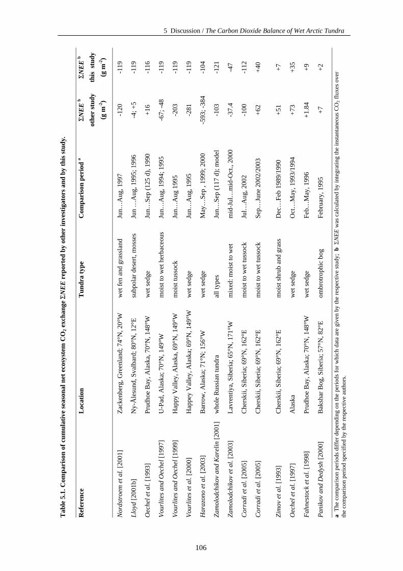
5 Discussion / The Carbon Dioxide Balance of Wet Arctic Tundra
ΣNE
E b
this
stu
dy
(g m
-2)
-119
-119
-116
-119
-119
-119
-104
-121
-47
-112
+40
+7
+35
+9
+2
ΣNE
E b
othe
r st
udy
(g m
-2)
-120
-4; +
5
+16
-67;
-48
-203
-281
-593
; -38
4
-103
-37.
4
-100
+62
+51
+73
+1.8
4
+7
Com
pari
son
peri
od a
Jun…
Aug
, 199
7
Jun
…A
ug, 1
995;
199
6
Jun…
Sep
(125
d),
1990
Jun…
Aug
, 199
4; 1
995
Jun…
Aug
199
5
Jun…
Aug
, 199
5
May
…Se
p , 1
999;
200
0
Jun…
Sep
(117
d);
mod
el
mid
-Jul
…m
id-O
ct.,
2000
Jul…
Aug
, 200
2
Sep…
June
200
2/20
03
Dec
…Fe
b 19
89/1
990
Oct
…M
ay, 1
993/
1994
Feb…
May
, 199
6
Febr
uary
, 199
5
Tun
dra
type
wet
fen
and
gras
slan
d
subp
olar
des
ert,
mos
ses
wet
sedg
e
moi
st to
wet
her
bace
ous
moi
st tu
ssoc
k
wet
sedg
e
wet
sedg
e
all t
ypes
mix
ed: m
oist
to w
et
moi
st to
wet
tuss
ock
moi
st to
wet
tuss
ock
moi
st sh
rub
and
gras
s
wet
sedg
e
wet
sedg
e
ombr
otro
phic
bog
Loc
atio
n
Zack
enbe
rg, G
reen
land
; 74°
N, 2
0°W
Ny-
Åle
sund
, Sva
lbar
d; 8
0°N
, 12°
E
Prud
hoe
Bay
, Ala
ska,
70°
N, 1
48°W
U-P
ad, A
lask
a; 7
0°N
, 149
°W
Hap
py V
alle
y, A
lask
a, 6
9°N
, 149
°W
Hap
pey
Val
ley,
Ala
ska;
69°
N, 1
49°W
Bar
row
, Ala
ska;
71°
N; 1
56°W
who
le R
ussi
an tu
ndra
Lavr
entiy
a, S
iber
ia; 6
5°N
, 171
°W
Che
rski
i, Si
beria
; 69°
N, 1
62°E
Che
rski
i, Si
beria
; 69°
N, 1
62°E
Che
rski
i, Si
beria
; 69°
N, 1
62°E
Ala
ska
Prud
hoe
Bay
, Ala
ska;
70°
N, 1
48°W
Bak
shar
Bog
, Sib
eria
; 57°
N, 8
2°E
Tab
le 5
.1. C
ompa
riso
n of
cum
ulat
ive
seas
onal
net
eco
syst
em C
O2 e
xcha
nge
ΣNE
E r
epor
ted
by o
ther
inve
stig
ator
s and
by
this
stud
y.
Ref
eren
ce
Nor
dstr
oem
et a
l. [2
001]
Lloy
d [2
001b
]
Oec
hel e
t al.
[199
3]
Vour
lites
and
Oec
hel [
1997
]
Vour
lites
and
Oec
hel [
1999
]
Vour
lites
et a
l. [2
000]
Har
azon
o et
al.
[200
3]
Zam
olod
chik
ov a
nd K
arel
in [2
001]
Zam
olod
chik
ov e
t al.
[200
3]
Cor
radi
et a
l. [2
005]
Cor
radi
et a
l. [2
005]
Zim
ov e
t al.
[199
3]
Oec
hel e
t al.
[199
7]
Fahn
esto
ck e
t al.
[199
8]
Pani
kov
and
Ded
ysh
[200
0]
a T
he c
ompa
rison
per
iods
diff
er d
epen
ding
on
the
perio
ds fo
r whi
ch d
ata
are
give
n by
the
resp
ectiv
e st
udy;
b Σ
NEE
was
cal
cula
ted
by in
tegr
atin
g th
e in
stan
tane
ous C
O2 f
luxe
s ove
r th
e co
mpa
rison
per
iod
spec
ified
by
the
resp
ectiv
e au
thor
s.
106
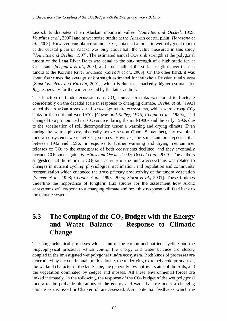
5 Discussion / The Coupling of the CO2 Budget with the Energy and Water Balance
tussock tundra sites at an Alaskan mountain valley [Vourlites and Oechel, 1999; Vourlites et al., 2000] and at wet sedge tundra at the Alaskan coastal plain [Harazono et al., 2003]. However, cumulative summer CO2 uptake at a moist to wet polygonal tundra at the coastal plain of Alaska was only about half the value measured in this study [Vourlites and Oechel, 1997]. The estimated annual CO2 sink strength at the polygonal tundra of the Lena River Delta was equal to the sink strength of a high-arctic fen at Greenland [Soegaard et al., 2000] and about half of the sink strength of wet tussock tundra at the Kolyma River lowlands [Corradi et al., 2005]. On the other hand, it was about four times the average sink strength estimated for the whole Russian tundra area [Zamolodchikov and Karelin, 2001], which is due to a markedly higher estimate for Reco, especially for the winter period by the latter authors.
The function of tundra ecosystems as CO2 sources or sinks was found to fluctuate considerably on the decadal scale in response to changing climate. Oechel et al. [1993] stated that Alaskan tussock and wet-sedge tundra ecosystems, which were strong CO2
sinks in the cool and wet 1970s [Coyne and Kelley, 1975; Chapin et al., 1980a], had changed to a pronounced net CO2 source during the mid-1980s and the early 1990s due to the acceleration of soil decomposition under a warming and drying climate. Even during the warm, photosynthetically active season (June…September), the examined tundra ecosystems were net CO2 sources. However, the same authors reported that between 1992 and 1996, in response to further warming and drying, net summer releases of CO2 to the atmosphere of both ecosystems declined, and they eventually became CO2 sinks again [Vourlites and Oechel, 1997; Oechel et al., 2000]. The authors suggested that the return to CO2 sink activity of the tundra ecosystems was related to changes in nutrient cycling, physiological acclimation, and population and community reorganization which enhanced the gross primary productivity of the tundra vegetation [Shaver et al., 1998; Chapin et al., 1995, 2005; Sturm et al., 2001]. These findings underline the importance of longterm flux studies for the assessment how Arctic ecosystems will respond to a changing climate and how this response will feed back to the climate system.
5.3 The Coupling of the CO2 Budget with the Energy and Water Balance – Response to Climatic Change
The biogeochemical processes which control the carbon and nutrient cycling and the biogeophysical processes which control the energy and water balance are closely coupled in the investigated wet polygonal tundra ecosystem. Both kinds of processes are determined by the continental, arctic climate, the underlying extremely cold permafrost, the wetland character of the landscape, the generally low nutrient status of the soils, and the vegetation dominated by sedges and mosses. All these environmental forces are linked intimately. In the following, the response of the CO2 budget of the wet polygonal tundra to the probable alterations of the energy and water balance under a changing climate as discussed in Chapter 5.1 are assessed. Also, potential feedbacks which the
107
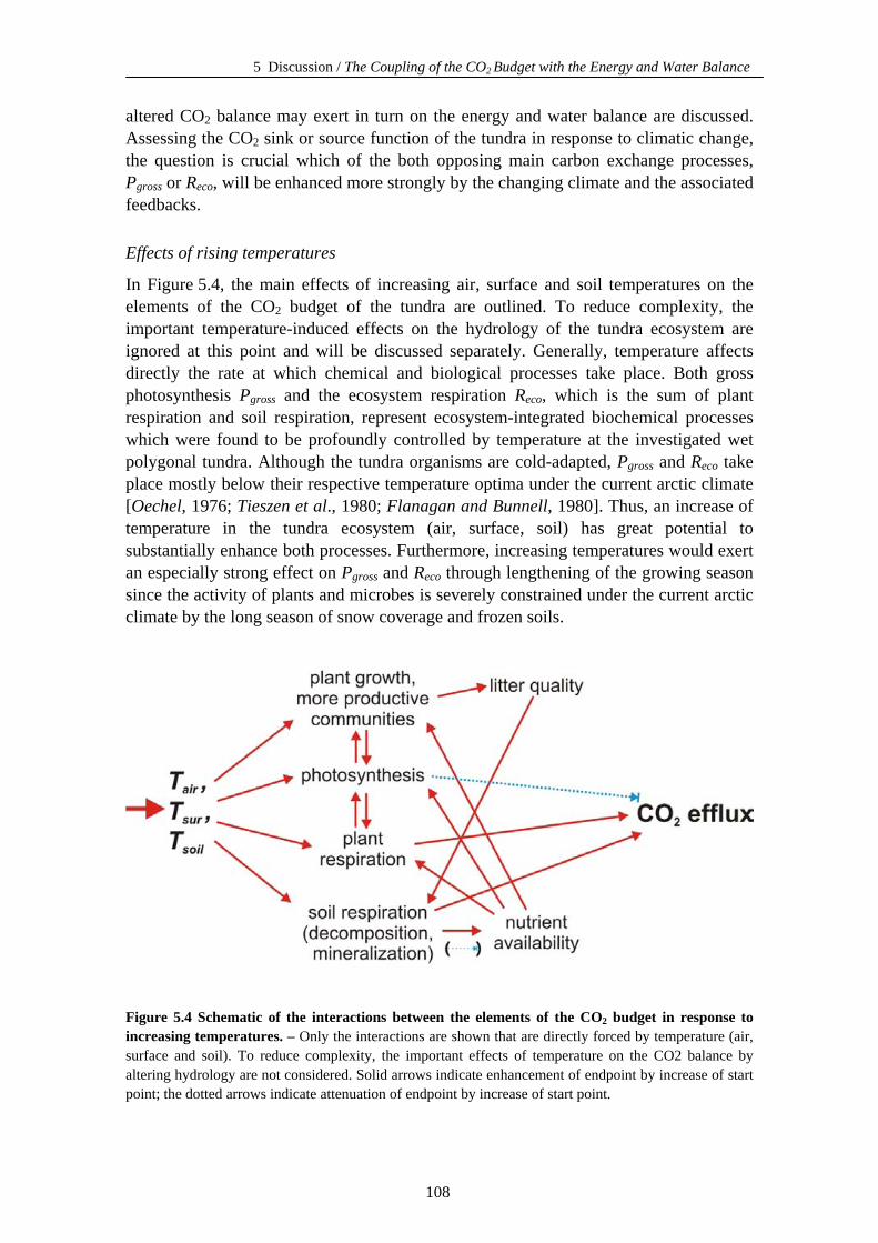
5 Discussion / The Coupling of the CO2 Budget with the Energy and Water Balance
altered CO2 balance may exert in turn on the energy and water balance are discussed. Assessing the CO2 sink or source function of the tundra in response to climatic change, the question is crucial which of the both opposing main carbon exchange processes, Pgross or Reco, will be enhanced more strongly by the changing climate and the associated feedbacks.
Effects of rising temperatures
In Figure 5.4, the main effects of increasing air, surface and soil temperatures on the elements of the CO2 budget of the tundra are outlined. To reduce complexity, the important temperature-induced effects on the hydrology of the tundra ecosystem are ignored at this point and will be discussed separately. Generally, temperature affects directly the rate at which chemical and biological processes take place. Both gross photosynthesis Pgross and the ecosystem respiration Reco, which is the sum of plant respiration and soil respiration, represent ecosystem-integrated biochemical processes which were found to be profoundly controlled by temperature at the investigated wet polygonal tundra. Although the tundra organisms are cold-adapted, Pgross and Reco take place mostly below their respective temperature optima under the current arctic climate [Oechel, 1976; Tieszen et al., 1980; Flanagan and Bunnell, 1980]. Thus, an increase of temperature in the tundra ecosystem (air, surface, soil) has great potential to substantially enhance both processes. Furthermore, increasing temperatures would exert an especially strong effect on Pgross and Reco through lengthening of the growing season since the activity of plants and microbes is severely constrained under the current arctic climate by the long season of snow coverage and frozen soils.
Figure 5.4 Schematic of the interactions between the elements of the CO2 budget in response to increasing temperatures. – Only the interactions are shown that are directly forced by temperature (air, surface and soil). To reduce complexity, the important effects of temperature on the CO2 balance by altering hydrology are not considered. Solid arrows indicate enhancement of endpoint by increase of start point; the dotted arrows indicate attenuation of endpoint by increase of start point.
108
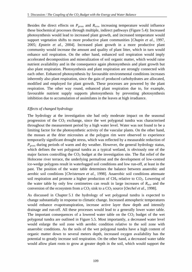
5 Discussion / The Coupling of the CO2 Budget with the Energy and Water Balance
Besides the direct effects on Pgross and Reco, increasing temperature would influence these biochemical processes through multiple, indirect pathways (Figure 5.4): Increased photosynthesis would lead to increased plant growth, and increased temperature would support vegetation shifts to more productive plant communities [Chapin et al., 1997, 2005; Epstein et al., 2004]. Increased plant growth in a more productive plant community would increase the amount and quality of plant litter, which in turn would enhance soil respiration. On the other hand, enhanced soil respiration would imply accelerated decomposition and mineralization of soil organic matter, which would raise nutrient availability and in the consequence again photosynthesis and plant growth but also plant respiration. Photosynthesis and plant respiration are strongly connected with each other. Enhanced photosynthesis by favourable environmental conditions increases inherently also plant respiration, since the gain of produced carbohydrates are allocated, modified and employed for plant growth. These processes are powered by the plant respiration. The other way round, enhanced plant respiration due to, for example, favourable nutrient supply supports photosynthesis by preventing photosynthesis inhibition due to accumulation of assimilates in the leaves at high irradiance.
Effects of changed hydrology
The hydrology at the investigation site had only moderate impact on the seasonal progression of the CO2 exchange, since the wet polygonal tundra was characterised throughout the measurement period by a high water level. Water was not found to be a limiting factor for the photosynthetic activity of the vascular plants. On the other hand, the mosses at the drier microsites at the polygon rim were observed to experience temporarily significant drought stress, which was reflected by a measurable reduction of Pgross during periods of warm and dry weather. However, the general hydrology status, which defines the wet polygonal tundra as a typical wetland, is obviously one of the major factors controlling the CO2 budget at the investigation site. The flat relief of the Holocene river terrace, the underlying permafrost and the development of low-centred ice-wedge polygons result in waterlogged soil conditions and low run-off, at least in the past. The position of the water table determines the balance between anaerobic and aerobic soil conditions [Christensen et al., 1998]. Anaerobic soil conditions attenuate soil respiration and promote a higher production of CH4 relative to CO2. Lowering of the water table by only few centimetres can result in large increases of Reco and the conversion of the ecosystem from a CO2 sink to a CO2 source [Oechel et al., 1998].
As discussed in Chapter 5.1 the hydrology of wet polygonal tundra is expected to change substantially in response to climatic change. Increased atmospheric temperatures would enhance evapotranspiration, increase active layer thaw depth and intensify drainage and run-off. All these processes would lead to a generally lower water table. The important consequences of a lowered water table on the CO2 budget of the wet polygonal tundra are outlined in Figure 5.5. Most importantly, a decreased water level would enlarge the soil zone with aerobic condition relative to the soil zone with anaerobic conditions. As the soils of the wet polygonal tundra have a high content of organic matter down to several meters depth, increased oxygen availability has the potential to greatly increase soil respiration. On the other hand, a decreased water table would allow plant roots to grow at greater depth in the soil, which would support the
109
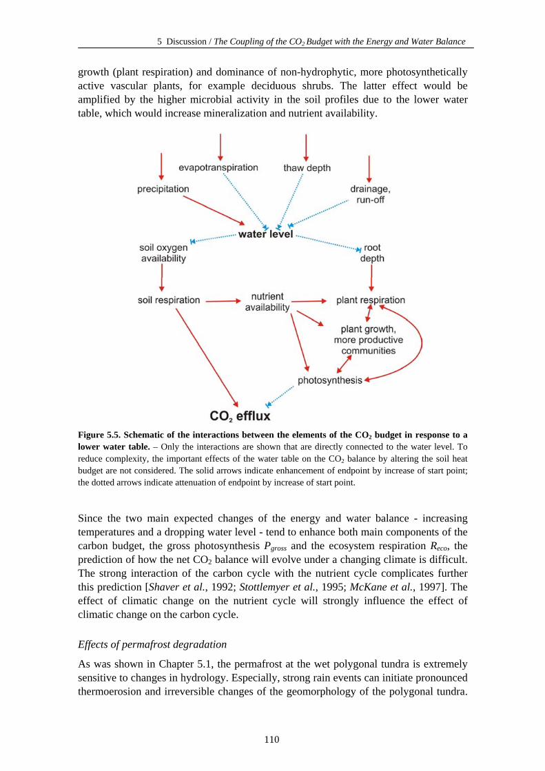
5 Discussion / The Coupling of the CO2 Budget with the Energy and Water Balance
growth (plant respiration) and dominance of non-hydrophytic, more photosynthetically active vascular plants, for example deciduous shrubs. The latter effect would be amplified by the higher microbial activity in the soil profiles due to the lower water table, which would increase mineralization and nutrient availability.
Figure 5.5. Schematic of the interactions between the elements of the CO2 budget in response to a lower water table. – Only the interactions are shown that are directly connected to the water level. To reduce complexity, the important effects of the water table on the CO2 balance by altering the soil heat budget are not considered. The solid arrows indicate enhancement of endpoint by increase of start point; the dotted arrows indicate attenuation of endpoint by increase of start point.
Since the two main expected changes of the energy and water balance - increasing temperatures and a dropping water level - tend to enhance both main components of the carbon budget, the gross photosynthesis Pgross and the ecosystem respiration Reco, the prediction of how the net CO2 balance will evolve under a changing climate is difficult. The strong interaction of the carbon cycle with the nutrient cycle complicates further this prediction [Shaver et al., 1992; Stottlemyer et al., 1995; McKane et al., 1997]. The effect of climatic change on the nutrient cycle will strongly influence the effect of climatic change on the carbon cycle.
Effects of permafrost degradation
As was shown in Chapter 5.1, the permafrost at the wet polygonal tundra is extremely sensitive to changes in hydrology. Especially, strong rain events can initiate pronounced thermoerosion and irreversible changes of the geomorphology of the polygonal tundra.
110
5 Discussion / The Coupling of the CO2 Budget with the Energy and Water Balance
Where thermoerosion is initiated, permafrost is rapidly thawed and destabilised. Degradation of permafrost has severe impacts on the carbon budget of the region. Large amounts of ancient carbon that have been stored in the permafrost sediments can be released from the permanently frozen and mostly anaerobic state and would be prone to decomposition. Substantial portions of the formerly frozen sediments including their large content of organic matter can be mobilised and transported to the lakes, rivers and ultimately to the Arctic Ocean. These drastic and irreversible changes that the polygonal tundra can experience due to climatic events have a great potential to increase the CO2 loss pronouncedly.
Changes of vegetation patterns
The change of the thermal, hydrological and geomorphological conditions in the Arctic will result in major shifts of the vegetation which will in turn exert pronounced feedbacks on the CO2, energy and water budget. Higher temperatures and longer growing seasons will allow the tree line to move distinctly northward thus reducing the tundra area [Scott et al., 1997; Everett and Fitzharris, 1998]. The energy balance of boreal forest is radically different compared to the energy balance of tundra [Bonan et al., 1995; Lafleur and Rouse, 1995; Harding et al., 2001]. A change of tundra to boreal forest would lead to lower albedo and higher net radiation -Qs*, lower relative ground heat flux QG, lower relative latent heat flux QE and higher relative sensible heat flux QH. The combination of these effects would promote further atmospheric warming. However, the northward movement of boreal forest may lag changes in temperature by decades to centuries [Chapin and Starfield, 1997].
But also changes within the tundra biome itself are of major importance for the energy and water budget of the Arctic. In response to increased temperature, drainage and desiccation, the vegetation communities of wet tundra, which consist mainly of sedges and mosses, would be replaced by communities adapted to moist to dry soil conditions which have a greater proportion of deciduous shrubs, herbs and grasses (Kutzbach et al., 2004a). The new plant communities probably would be taller and will have a larger photosynthetically active leaf area than the former vegetation. The result would be a higher gross primary productivity and an increased carbon storage in plant biomass. Furthermore, the change from mosses and sedges to grasses, herbs and deciduous shrubs would affect nutrient availability and soil respiration by better litter quality. Taller and more complex canopies are characterised by a higher roughness length and a larger leaf area which represents the principal exchange surface between the terrestrial ecosystems and the atmosphere. Thus, a change from the rather low-statured sedge- and moss-dominated vegetation of the polygonal tundra to taller vegetation types would accelerate the exchange of momentum, energy, water and carbonaceous gases with the atmosphere.
Especially the expansion of deciduous shrubs in tundra, an effect that is already underway on a large scale [Myeni et al., 1997; Sturm et al., 2001a; Epstein et al., 2004], would have strong impacts on the energy, water and CO2 budget of tundra. Shrubs trap and hold very effectively drifting snow which leads to increased snow pack heights, better insulation of the soils and less sublimation [McFadden et al., 2001]. The resulting
111
5 Discussion / The Coupling of the CO2 Budget with the Energy and Water Balance, Perspectives
higher soil temperatures promote microbial mineralisation and further shrub growing. Since shrubs are the tundra plants with the highest wood content, which is characterised by a high C/N value, an increase of shrub abundance can enhance the nitrogen efficiency of carbon sequestration of the tundra vegetation. This snow-shrub-soil-microbe positive feedback loop was described elaborately by Sturm et al. [2001b, 2005]. Additionally, the increasing shrub density decreases the albedo in summer as well as in winter when the dark shrub branches protrude above the snow thus enhancing the energy uptake by the tundra ecosystem [Chapin et al., 2005]. However, the increased snow depth by the spreading of shrubs represents also a negative feedback on the annual energy and CO2 budget because the higher snow pack will probably result in a longer snow ablation period in spring and a later start of the growing season.
5.4 Perspectives Although important new insights in the energy, water and CO2 exchange between wet arctic tundra and the atmosphere were gained by this study, there remain many open questions, which point out areas where further research is necessary in the future.
The carbon balance of the wet polygonal tundra is not complete with the study of CO2, because the Arctic wetland is also a major source of methane (CH4). Methane is an important radiatively active trace gas, second only to CO2 in its cumulative effect on the additional anthropogenic greenhouse effect. On a mole basis, CH4 is about 25 times more effective as a greenhouse gas than CO2 [Rohde, 1990].
During the micrometeorological campaigns 2003 and 2004, also the ecosystem exchange of this important trace gas was measured by the eddy covariance method. The fluctuations of the CH4 concentration were measured by a CH4 analyser based on tuneable diode laser infrared absorption spectroscopy (TDL; TGA 100, Campbell Scientific Ltd., USA, Figure 3.2). The time series of the CH4 exchange fluxes during the measurement campaign 2003 are shown in Figure 5.6 along with the progression of soil temperature (polygon centre, 20 cm depth), which is a main control on CH4 production. The CH4 flux ranged between 0.2 mg CH4 h-1 m-2 and 5.4 mg CH4 h-1 m-2 during the campaign 2003 (July 20…October 21). The mean CH4 flux amounted to (0.8 ± 0.5) mg CH4 h-1 m-2 (median 0.7 mg CH4 h-1 m-2). The mean release of carbon as CH4 was 0.6 mg C h-1 m-2 which is 2.4 % of the mean carbon release as CO2 by the ecosystem respiration Reco (24.5 mg C h-1 m-2) during the same period.
The CH4 fluxes determined by the eddy covariance method were well comparable with CH4 fluxes measured by means of a closed chamber technique at the polygonal tundra of the Lena River Delta [Wagner et al., 2003b]. The latter authors reported CH4 fluxes of 0.2 mg CH4 h-1 m-2 for the polygon rims and 2.2 mg CH4 h-1 m-2 for the polygon centres, which would result in an area-weighted average of about 1.0 mg CH4 h-1 m-2 for the fetch of the eddy covariance measurements (~60 % of the total area rim, ~40 % of the area centre).
112

5 Discussion / Perspectives
However, the measurements of the CH4 fluxes were prone to a range of technical and logistical problems which led to a heavily fragmented time series of the CH4 fluxes. During the campaign 2003, 44 % of the 30 min measurement intervals had to be dismissed due to technical problems (Table 3.2); during the campaign 2004 even 80 % had to be excluded. These methodical problems compromised a thorough evaluation of the CH4 exchange fluxes. Nevertheless, much work was done in the last three years to improve the performance of the turbulent CH4 flux measurements, and the preliminary results of the micrometeorological campaign in the Lena River Delta during the summer 2005 are promising. This positive development opens the possibility of a complete study of the carbon exchange between the wet tundra and the atmosphere in the future.
Figure 5.6. Time series of CH4 fluxes (A) and soil temperature (B) during the campaign 2003. – A The data points represent CH4 fluxes FCH4 measured by the eddy covariance method over 30 min intervals. B The soil temperature TS-20cm was measured at the polygon centre at 20 cm depth.
In addition to the measurements of vertical carbon exchange fluxes as CO2 or CH4, research on the lateral fluxes of carbon as dissolved CO2, CH4 or dissolved organic matter is necessary for an assessment of the complete carbon balance of the tundra ecosystem [Gundelwein, 1998]. Another important topic for future research would be the analysis of the interconnections between the carbon balance and the nutrient (nitrogen, phosphorus) budget of the permafrost soils. The nutrient cycling plays a major role in the coupling of gross photosynthesis and ecosystem respiration to the energy and water budget (Figure 5.4, Figure 5.5).
Since the respiration as well as the CH4 production during wintertime can be a substantial component of the annual carbon balance in arctic ecosystems, CO2 and CH4 flux measurement campaigns throughout the winter are highly desirable. Also, direct
113
5 Discussion / Perspectives
measurements of wintertime sublimation are required to close a major gap in the knowledge about the annual water balance at Siberian tundra. Furthermore, if we aim at accurately assessing the response of the energy, water and carbon balance to climatic change, longterm studies are needed because the interannual variability of climate and the investigated ecosystem-atmosphere exchange processes is high.
A special focus should be set on permafrost degradation and irreversible changes within the tundra ecosystem due to thermoerosion and thermokarst phenomena. The polygonal tundra of the Lena River Delta has been observed to react very sensitive to thermoerosion due to hydrology changes, and the implications of such irreversible changes for the carbon balance are drastic.
The wet polygonal tundra in the Lena River Delta is characterised by a high small-scale spatial variability of soils, hydrology and vegetation. The eddy covariance method determines the ecosystem exchange fluxes on the larger (ecosystem) scale of several hectares to square-kilometres. The influence of the small-scale spatial variability on the eddy covariance flux measurements should be evaluated in more detail in the future. Therefore, the small-scale variability of the soil-meteorological variables as well as the radiation components and the snow height should be monitored at higher spatial density within the fetch of the eddy covariance measurements. Especially the properties and processes of the many small water bodies within the polygonal tundra should be investigated, since they obviously differ strongly from the soils. Questions of geo-statistics, homogeneity, representativeness and upscaling problems should be addressed [Schmidt, 1997]. For these purposes, the spatial variability of surface conditions on the various scales should be analysed by using remote sensing data from various platforms (satellite, airplane, kite or small zeppelin). In combination with the micrometeorological flux measurements, the energy, water and carbon fluxes should be investigated on the microsite scale, for instance by chamber gas flux measurements, to improve the process understanding. For instance, the net ecosystem CO2 exchange NEE, which is directly measured by the eddy covariance method, is the balance of a range of biological processes including photosynthesis, aboveground plant respiration, root respiration and microbial respiration. As shown in this study, much information about the single processes of the CO2 budget can be derived by the eddy covariance method. However, a more detailed insight in the main processes of the energy, water and carbon budget is often desirable, especially for modelling purposes.
The carbon balance of tundra ecosystems is controlled by a complex network of interacting environmental factors and processes. Many of the single biogeochemical and biogeophysical processes are recognised and rather well understood. However, the understanding of the single processes does not suffice to predict the response of the complex system as a whole to changing environmental conditions. Therefore, further intense field studies should be combined with the development or adjustment of a comprehensive and detailed process-based model for the specific regional conditions of wet polygonal tundra of the Lena River Delta. The model has to consider and combine the biogeochemical processes, e.g. photosynthesis, plant growth, plant and microbial respiration, and the biogeophysical processes related to the energy and water balance, e.g. evapotranspiration, soil heat budget, active-layer thawing and soil hydrology.
114
6 Conclusions
6 Conclusions This study demonstrated that the North-Siberian wet arctic tundra differs considerably from tundra ecosystems in North-America and Europe regarding the energy and water budget as well as the CO2 balance. Therefore, the intensification of biogeochemical and biogeophysical research in the extensive tundra landscapes of Siberia is urgently needed for a better understanding of the arctic carbon cycle and the arctic climate. This study delivered a range of new results on the processes of the energy, water and CO2 cycling at wet arctic tundra of Northern Siberia which are considered to be of concern not only for the Lena River Delta but also for the extensive area of the North Siberian lowland tundra as a whole. The results of this investigation represent a high-quality data set which will be integrated in the international CO2 exchange network FLUXNET and has great potential for improving the land-atmosphere parameterisation schemes of regional and global climate models. On the basis of the presented results and discussions, the following main conclusions are drawn:
The eddy covariance method was successfully used to characterise the ecosystem-scale exchange of energy, water and CO2 between wet arctic tundra and the atmosphere. The relative energy balance closure was around 90 % on the hourly basis and around 96 % on the daily basis, indicating good system performance.
The energy and water balance at the investigated tundra is determined by (1.) the polar and distinctly continental climate, (2.) the very cold and ice-rich permafrost which underlies the tundra of Northern Siberia, (3.) the wetland character of polygonal tundra, (4.) the position at the interface between the Arctic Ocean and the Siberian hinterland, and (5.) the long duration of the snow coverage.
The CO2 budget of the investigated tundra is closely coupled with the energy and water balance at the site. Thus, the abovementioned main driving forces of the energy and water balance are also major controls on the CO2 budget. Additionally, the CO2 budget is strongly influenced by (6.) the generally low nutrient status of the soils at the site and (7.) a vegetation dominated by sedges and mosses.
The exchange fluxes of energy, water and CO2 show clear seasonal trends on which the diurnal oscillation and pronounced meso-scale variations, which are related to the prevailing synoptic weather conditions, are superimposed. The synoptic weather conditions affect strongly the exchange fluxes by changes in cloudiness, precipitation and the advection of air masses from either the Siberian hinterland or the Arctic Ocean. Thus, the development of the large-scale atmospheric circulation patterns, for example the phase of the Arctic Oscillation, has a strong influence on the function of the North-Siberian tundra as a sink or source of heat, water and CO2.
The duration of the snow-covered period is a major control on the seasonal and annual energy, water and CO2 balance. During the snow-covered period, the net radiation is either directed away from the surface (autumn/winter) or directed towards the surface with only low values due to the high albedo of snow (late spring). The low available energy during snow coverage leads to low values of ground heat flux and latent heat
115
6 Conclusions
flux. The sensible heat flux is mostly directed from the atmosphere towards the surface during the snow-covered period. The main CO2 exchange processes, namely the ecosystem respiration and the gross photosynthesis, are low due to frozen soils and insufficient light under the snow pack.
The comparison between winter snowfall data and spring snow heights and density suggests a major winter water loss from the snow pack to the atmosphere by sublimation. Sublimation from the snow pack is a major uncertainty in the annual water and energy budget and should be studied in detail in the future.
During the short snow-free period (June…September), the exchange of energy, water and CO2 between the tundra and the atmosphere is most intensive. The cumulative summer energy partitioning is characterised by low net radiation (607 MJ m-2), large ground heat flux (163 MJ m-2), low latent heat flux (250 MJ m-2) and very low sensible heat flux (157 MJ m-2) compared to other tundra sites. These findings point out the major importance of the very cold permafrost (due to extreme winter cooling) for the summer energy budget of the tundra in Northern Siberia. The partitioning of the available energy into latent and sensible heat fluxes is typical for arctic wetlands as indicated by the Bowen ratio, which ranged between 0.5 and 1.5 during most of the summer. Continuous light conditions during midsummer (polar day) do not prevent diurnal variations of the energy fluxes. On the contrary, the diurnal variations of the energy fluxes are most pronounced during midsummer and diminish with approaching autumn.
Despite high input of water as rainfall (201 mm) or snow melt water, the cumulative evapotranspiration during summer (June…August) was with 98 mm (mean (1.1 ± 0.7) mm d-1) low compared to other tundra sites. The water exchange between the arctic wetland and the atmosphere is normally limited by the low available energy and only seldom constrained by low water availability. Accordingly, the average decoupling factor Ω of 0.53 ± 0.13 indicates a relatively low coupling of the atmosphere and the vegetation compared to other tundra sites. However, the surface resistance to evapotranspiration can increase significantly during longer periods of advection of warm and dry air from the South due to water stress of the mosses at the drier microsites of the polygon rims.
The heavy rainfall in summer 2003 initiated severe thermoerosion phenomena and in consequence increased drainage and run-off at the wet polygonal tundra. Wet polygonal tundra has to be considered as very sensitive to changes in hydrology, especially to high-intensity rainfall events. Because of this effect, the predicted rise of precipitation due to global change will probably not lead to higher soil moisture but rather to lower water levels and drier soils. The impacts of thermoerosion lead to rapid and irreversible perturbations of the tundra landscape. Considering the large amount of carbon in the permafrost which may be released when permafrost is degraded, these effects represent major positive feedbacks on the warming climate.
The CO2 budget of the wet polygonal tundra is characterised by a low intensity of the main CO2 exchange processes between the ecosystem and the atmosphere, namely the gross photosynthesis Pgross and the ecosystem respiration Reco. Both processes are
116
6 Conclusions
attenuated by the unfavourable environmental conditions at the site, which include climatic as well as pedogenetic factors.
The cumulative Pgross amounted to -432 g m-2 over the photosynthetically active period (June...September). The rather low Pgross is related to the low coverage of vascular plants, mainly sedges, and the high coverage of the mosses at the polygonal tundra. The contribution of moss photosynthesis to the annual Pgross is estimated to be about 40 %. The gross primary productivity of the vegetation of the wet polygonal tundra is constrained by the low nutrient availability in the soils.
The diurnal response of Pgross is mainly controlled by the irradiation. Although the irradiance is the limiting factor during the night, during midday the photosynthetic apparatus of the canopy is frequently near saturation and represents the limiting factor on Pgross. The seasonal progression of Pgross is controlled by the combination of the phenological development of the vegetation and the general temperature progression over the summer. The phenological development of the plants is largely controlled by intrinsic factors. However, temperature is also a major control on Pgross at the investigation site since photosynthesis takes place for most of the time below its temperature optimum. On the other hand, water availability has only minor importance as control on Pgross due to the wet soil conditions at polygonal tundra. Only when the mosses at the drier microsites of the polygon rim experience water stress, Pgross is reduced significantly.
The cumulative Reco amounted to +327 g m-2 over the photosynthetically active period (June…September), which corresponds to 76 % of the cumulative Pgross. However, Reco continues at substantial rates during autumn when photosynthesis has ceased and the soils are still largely unfrozen and to a lesser degree throughout the winter and spring. The significant Reco during autumn, winter and spring is a major but highly uncertain factor in the annual CO2 balance which should be addressed in future winter campaigns. The temporal variability of Reco during summer is best explained by the surface temperature and not by the soil temperature. This finding demonstrates the high and often overlooked importance of the autotrophic plant respiration within the CO2 balance. Indeed, the composition and productivity of the vegetation have to be considered as major controls on Reco.
Under the current arctic climate, the wet polygonal tundra of the Lena River Delta acts as a CO2 sink with a cumulative net ecosystem CO2 exchange NEE of -119 g m-2 over the summer (June…August) and an estimated annual NEE of -71 g m-2. Also a more complete carbon balance, including the release of CH4 from the ecosystem to the atmosphere, will probably result in a clear carbon sink function of the investigated wet arctic tundra since the carbon release as CH4 can be estimated to amount to only about 2 %…3 % of the carbon release as CO2 by Reco. Nevertheless, the study of the CH4 exchange between tundra and the atmosphere remains highly important because the artic wet tundra ecosystems are a globally important source of this very effective greenhouse gas.
The analysis of the qualitative relationships between the involved processes and environmental factors suggests that the wet arctic tundra will experience severe perturbations in consequence of the predicted climatic change. The alterations of the
117

6 Conclusions
tundra ecosystems will in turn exert pronounced feedbacks on the changing climate on the regional and global scale.
The presented thought experiments demonstrate the complex nature of the interactions between the energy and water budget and the CO2 balance. However, the quantitative assessment of how this network of interconnected driving factors and coupled processes will react to climate change is only possible by combining further intense field studies on the biogeochemical and biogeophysical processes with the development or adjustment of elaborate process-based models. These models have to consider explicitly the special conditions at North-Siberian tundra ecosystems.
118
7 References
7 References ACIA. 2004. Impacts of a Warming Arctic: Arctic Climate Impact Assessment. Cambridge University
Press, New York, USA.
ALABYAN AM, CHALOV RS, KOROTAEV VN, SIDORCHUK AY, ZAITSEV AA. 1995. Natural and technigenic water and sediment supply to the Laptev Sea. Reports on Polar Research 176: 265-271.
ALLEN RG, JENSEN ME, WRIGHT JL, BURMAN RD. 1989. Operational estimates of evaporation. Agron J 81: 650-662.
ALM J, TALANOV A, SAARNIO S, SILVOLA J, IKKONEN E, AALTONEN H, NYKÄNEN H, MARTIKAINEN PJ. 1997. Reconstruction of the carbon balance for microsites in a boreal oligotrophic pine fen, Finland. Oecologia 110: 423-431.
ANISIMOV OA, SHIKLOMANOV NI, NELSON FE. 1997. Global warming and active-layer thickness: results from transient general circulation models. Global Planetary Change 15: 61-77.
ANISIMOV OA., VELICHKO AA, DEMCHENKO PF, ELISEEV AV, MOKHOV II, NECHAEV VP. 2002. Effect of climate change on permafrost in the past, present, and future. Izvestiya, Atmospheric and Oceanic Physics 38(1): 25-39.
ARE FE, REIMNITZ E. 2000. An overview of the Lena River Delta setting: geology, tectonics, geomorphology, and hydrology. J Coastal Res 16(4): 1083-1093.
AUBINET M, GRELLE A, IBRON A, RANNIK Ü, MONCRIEFF J, FOKEN T, KOWALSKI AS, MARTIN PH, BERBIGIER P, BERNHOFER C, CLEMENT R, ELBERS J, GRANIER A, GRÜNWALD T, MORENSTERN K, PILEGAARD K, REBMANN C, SNIJDERS W, VALENTINI R, VESALA T. 2000. Estimates of the annual net carbon and water exchange of forests: the EUROFLUX methodology. Adv Ecol. Research 30: 113-175.
AURELA M, TUOVINEN J-P, LAURILA T. 2001. Net CO2 exchange of a subarctic mountain birch ecosystem. Theor Appl Climatol 70: 135-148.
BALDOCCHI D, VALENTINI R, RUNNING S, OECHEL WC, DAHLMAN R. 1996. Strategies for measuring and modelling carbon dioxide and water vapour fluxes over terrestrial ecosystems. Global Change Biol 2: 159-168.
BALDOCCHI DD. 2003. Assessing the eddy covariance technique for evaluating carbon dioxide exchange rates of ecosystems: past, present and future. Global Change Biol 9: 479-492.
BALOBAEV VT. 1997. Thermal interaction between the atmosphere and permafrost and their water budget. In: Fukushima Y and Ohata T (eds) Proceedings of International Workshop on Energy and Water Cycle in GAME-Siberia, 1995. Institute for Hydrospheric-Atmospheric Sciences, Nagoya University, Nagoya, Japan.
BARNOLA JM, ANKLIN M, PORCHERON J, RAYNAUD D, SCHWANDER J, STAUFFER B. 1995. CO2 evolution during the last millennium as recorded by Antarctic and Greenland ice. Tellus B 47: 264-272.
BECKER H, AKHMADEEVA I, WAGNER D, PFEIFFER E-M., Quass W. 1999. Soils of Samoylov Island. In: Rachold V (ed) Expeditions in Siberia in 1998. Reports on Polar Research 315. Alfred Wegener Institute, Bremerhaven, Germany, pp 21-27.
BERNER U, STREIF H (eds). 2001. Klimafakten. Der Rückblick, ein Schlüssel für die Zukunft. 3rd edition. Schweizerbartsche Verlagsbuchhandlung, Stuttgart, Germany, 238 pp (in German).
119
7 References
BERINGER J, TAPPER NJ, MCHUGH I, CHAPIN FS III, LYNCH AH, SERREZE MC, SLATER A. 2001. Impact of Arctic treeline on synoptic climate. Geophys Res Lett 28(22): 4247-4250.
BIASI C, MEYER H, RUSALIMOVA O, KAISER C, WANEK W, BARSUKOV P, RICHTER A. 2004. Temperature-dependent shift from labile to recalcitrant carbon sources of arctic heterotrophs. Talk with published abstract at the Joint European Stable Isotope Users Group Meeting (JESIUM), 30 August - 3 September, 2004, Vienna, Austria.
BILLINGS WD. 1987. Carbon balance of Alaskan tundra and taiga ecosystems: past, present and future. Quatern Sci Rev 6: 165-177.
BILLINGS WD, PETERSON KM, SHAVER GR, TRENT AW. 1977. Root growth, respiration, and carbon dioxide evolution in an arctic tundra soil. Arct Alp Res 9(2): 129-137.
BOIKE J. 2005. Unpublished meteorological and soil-meteorological data. Alfred Wegener Institute for Polar and Marine Research, Telegrafenberg A43, 14471 Potsdam, Germany
BOIKE J, OVERDUIN PP. 1999. Seasonal changes in hydrology, energy balance, and chemistry in the active layers of Arctic Tundra soils in Taymyr Peninsula, Russia. In: Kassens et al. (eds) Land-ocean systems in the Siberian Arctic: Dynamics and history, Lecture notes in earth science. Springer, Berlin, Germany, pp 299-306.
BOIKE J, ROTH K, OVERDUIN PP. 1998. Thermal and hydrologic dynamics of the active layer at a continuous permafrost site (Taymyr Peninsula, Siberia). WaterResources Research 34(3): 355-363.
BOIKE J, ROTH K, IPPISCH O. 2003a. Seasonal snow cover on frozen ground: Energy balance calculations of a permafrost site near Ny-Ålesund, Spitsbergen. J Geophys Res 10:
BOIKE J, HINZMAN L, OVERDUIN PP, ROMANOVSKY V, IPPISCH O, ROTH K. 2003b. A comparison of snow melt at three circumpolar sites: Spitsbergen, Siberia, Alaska. Poster at the 8th International Conference on Permafrost, 21-25th July, Zurich, Switzerland.
BOLTZMANN L. 1884. Ableitung des Stefan'schen Gesetzes, betreffend die Abhängigkeit der Wärmestrahlung von der Temperatur aus der electromagnetischen Lichttheorie. Annalen der Physik und Chemie 22: 291-294.
BONAN GB, CHAPIN FS III, THOMPSON SL. 1995. Boreal forest and tundra ecosystems as components of the climate system. Climatic Change 29: 145-167.
BOWEN IS. 1926. The ratio of heat losses by conduction and by evaporation from any water surface. Phys Rev 27: 779–787.
BRAMER H. 1982. Geographische Zonen der Erde. VEB Hermann Haack, Gotha. 128 pp.
BRIGGS D, SMITHSON P. 1994: Fundamentals of Physical Geography. Routledge, London.
BRINKOP S, ROECKNER E. 1995. Sensitivity of a general circulation model to parameterizations of cloud-turbulence interactions in the atmospheric boundary layer. Tellus 47A: 197-220.
BROECKER WS. 1997. Thermohaline circulation, the Achilles heel of our climate system: Will man-made CO2 upset the current balance? Science 278: 1582-1588.
BROTZGE JA, DUCHON CE. 2000. A Field Comparison among a Domeless Net Radiometer, Two Four-Component Net Radiometers, and a Domed Net Radiometer. J Atmos Ocean Tech 17(12): 1569-1582.
BROWN J, EVERETT KR, WEBBER PJ, MACLEAN SF JR, MURRAY DF. 1980. The coastal tundra at Barrow. In: Brown et al (eds) An Arctic Ecosystem: the Coastal Tundra at Barrow, Alaska. Dowden, Hutchinson & Ross Inc, Stroudsburg, PA, USA. pp 1-29.
BUCHMANN N, SCHULZE E-D. 1999. Net CO2 and H2O fluxes of terrestrial ecosystems. Global Biogeochem Cycles 13: 751-760.
120
7 References
BUCK AL. 1981. New equations for computing vapour pressure and enhancement factor. J Appl Meteorol 20: 1527-1532.
CALLAGHAN TV, JONASSON S. 1995. Implications for changes in arctic plant biodiversity from environmental manipulation experiments. In: Chapin FS III and Körner CH (eds) Arctic and Alpine Biodiversity: Patterns, Causes, and Ecosystem Consequences. Springer-Verlag, Heidelberg, Germany, pp 151-164.
CAMPBELL SCIENTIFIC INC. 2003. NR-LITE Net Radiometer Instruction Manual. Campbell Scientific Inc, Logan, UT, USA. 14 pp.
CAMPBELL SCIENTIFIC INC. 2004. TGA100A Trace Gas Analyser Overview. Campbell Scientific Inc, Logan, UT, USA. 14 pp.
CHAPIN FS III, MILLER PC, BILLINGS WD, COYNE PI. 1980a. Carbon and nutrient budgets and their control in coastal tundra. In: Brown et al (eds) An Arctic Ecosystem: the Coastal Tundra at Barrow, Alaska. Dowden, Hutchinson & Ross Inc, Stroudsburg, PA, USA. pp 458-482.
CHAPIN FS III, TIESZEN LL, LEWIS MC, MILLER PC, MCCOWN BH. 1980b. Control of tundra plant allocation patterns and growth. In: Brown et al (eds) An Arctic Ecosystem: the Coastal Tundra at Barrow, Alaska. Dowden, Hutchinson & Ross Inc, Stroudsburg, PA, USA. pp 140-185.
CHAPIN FS III, JEFFRIES RL, REYNOLDS JF, SHAVER GR, SVOBODA J. 1992. Arctic Ecosystems in a Changing Climate: an Ecophysiological Perspective. Academic Press, San Diego, USA.
CHAPIN FS III, SHAVER GR, GIBLIN AE, NADELHOFFER KG, LAUNDRE JA. 1995. Responses of Arctic tundra to experimental and observed changes in climate. Ecology 76: 694-711.
CHAPIN FS III, STARFIELD AM, 1997: Time lags and novel ecosystems in response to transient climatic change in arctic Alaska. Climatic Change 35, 449-461.
CHAPIN FS III, MCFADDEN JP, HOBBIE SE. 1997. The role of arctic vegetation in ecosystem and global processes. In: Woodin SJ and Marquiss M (eds) Ecology of Arctic Environments. Blackwell Science, Oxford, UK, pp 97-112.
CHAPIN FS III, STURM M, SERREZE MC, MCFADDEN JP, KEY JR, LLOYD AH, MCGUIRE AD, RUPP TS, LYNCH AH, SCHIMEL JP, BERINGER J, CHAPMAN WL, EPSTEIN HE, EUSKIRCHEN ES, HINZMAN LD, JIA G, PING CL, TAPE KD, THOMPSON CDC, WALKER DA, WELKER JM. 2005. Role of Land-Surface Changes in Arctic Summer Warming. Science Express: DOI: 10.1126/science.1117368
CHAPMAN WL, WALSH JE. 1993. Recent Variations of Sea Ice and Air Temperature in High Latitudes. Bull Am Meteorol Soc 74(1): 33–47.
CHRISTENSEN T. 1993. Methane emission from arctic tundra. Biogeochemistry 21: 117-139.
CHRISTENSEN TR, JONASSON S, MICHELSEN A, CALLAGHAN TV, HAVSTRÖM M. 1998. Environmental controls on soil respiration in the Eurasian and Greenlandic Area. J Geophys Res 103(D22): 29015-29021.
CHRISTENSEN TR, JOHANSSON T, ÅKERMAN HJ, MASTEPANOV M, MALMER N, FRIBORG T, CRILL P, SVENSSON BH. 2004. Thawing sub-arctic permafrost: Effects on vegetation and methane emissions. Geophys Res Lett 31: L04501, doi:10.1029/2003GL018680.
CLARK PU, PISIAS NG, STOCKER TF, WEAVER AJ. 2002. The role of the thermohaline circulation in abrupt climate change. Nature 415: 863-869.
COOK RB, HOLLADAY SK, GU L, HORWEDEL BM, JACKSON BL, BODEN TA, FALK M, BALDOCCHI D. 2004. A global network of eddy-covariance flux towers. Presentation at the AmeriFlux Annual Meeting. Available on-line [http://www.fluxnet.ornl.gov/fluxnet/present.cfm] from ORNL DAAC, Oak Ridge, Tennessee, U.S.A. Accessed January 29, 2005.
121
7 References
COYNE PI, KELLEY JJ. 1975. CO2 exchange over the Alaskan arctic tundra: meteorological assessment by an aerodynamic method. J Appl Ecol 12: 587-611.
DAI A, DELGENIO AD, FUNG IY, 1997. Clouds, precipitation, and temperature range. Nature 386: 665-666.
CORRADI C, KOLLE O, WALTER K, ZIMOV SA, SCHULZE E-D. 2005. Carbon dioxide and methane exchange of a north-east Siberian tussock tundra. Global Change Biol 11: 1-16, doi: 10.1111/j.1365-2486.2005.01023.x
CURRY JA, ROSSOW WB, RANDALL D, SCHRAMM JL. 1996. Overview of Arctic cloud and radiation characteristics. J Climate 9: 1731-1764.
DETHLOFF K, RINKE A, LEHMANN R, CHRISTENSEN JH, BOTZET M, MACHENHAUER B. 1996. Regional Climate Model of the Arctic Atmosphere. J Geophys Res 101: 23401-23422.
DETHLOFF K, WEISHEIMER A, RINKE A, KURGANSKY MV, JANSEN W, MAAß P, HUPFER P. 1998. Climate variability in a nonlinear atmosphere-like dynamical system. J Geophys Res 103: 25,957-25,966.
DE VRIES DA. 1963. Thermal properties of soils. In: van Wijk (ed) Physics of Plant Environment. North-Holland Publishing Co, Amsterdam, The Netherlands.
DEN HARTOG G, NEUMANN HH, KING KM, CHIPANSHI AC. 1994. Energy budget measurements using eddy correlation and Bowen ratio techniques at the Kinosheo Lake tower site during the Northern Wetlands Study. J Geophys Res 99(D1): 1539-1549.
DORN W, DETHLOFF K, RINKE A, BOTZET M. 2000. Distinct circulation states of the Arctic atmosphere induced by natural climate variability. J Geophys Res 105: 29,659-29,668.
EATON AK, ROUSE WR, LAFLEUR PM, MARSH P, BLANKEN PD. 2001. Surface energy balance of the western and central Canadian subarctic: variations in the energy balance among five major terrain types. J Climate 14: 3692-3703.
EDWARDS GC, NEUMANN HH, DEN HARTOG G, THURTELL GW, KIDD G. 1994. Eddy correlation measurements of methane fluxes using a tunable diode laser at the Kinosheo Lake tower site during the Northern Wetlands Study (NOWES). J Geophys Res 99(D1): 1511-1518.
EPSTEIN HE, CALEF MP, WALKER MD, CHAPIN FS III, STARFIELD AM. 2004. Detecting changes in arctic plant communities in response to warming over decadal time scales. Global Change Biology 10:1325-1334.
ELOVSKAYA LG. 1987. Classification and diagnostics of Yakutian permafrost soils. Yakutian Section of the Siberian Branch of the Academy of Science USSR, Yakutsk.
ETHERIDGE DM, STEELE LP, FRANCEY RJ, LANGENFELDS RL. 1998. Atmospheric methane between 1000 A.D. and present: Evidence of anthropogenic emissions and climatic variability. J Geophys Res 103: 15979-15993.
EUGSTER W, MCFADDEN JP, CHAPIN FS III. 1997. A comparative approach to regional variation in surface fluxes using mobile eddy correlation towers. Boundary-Layer Meteorol 85: 293-307.
EUGSTER W, ROUSE WR, PIELKE RA SR, MCFADDEN JP, BALDOCCHI DD, KITTEL TG, CHAPIN FS III, LISTON GE, VIDALE PL, VAGANOV E, CHAMBERS S. 2000. Land-atmosphere energy exchange in Arctic tundra and boreal forest: available data and feedbacks to climate. Global Change Biol 6(S1): 84-115.
EVERETT JT, FITZHARRIS BB. 1998. The Arctic and Antarctic. In: Watson RT, Zinyowera MC, Moss RH (eds) The Regional Impacts of Climate Change: An Assessment of Vulnerability. Cambridge University Press, Cambridge, UK. pp 85-103.
FAHNESTOCK JT, JONES MH, BROOKS PD, WALKER DA, WELKER JM. 1998. Winter and early spring CO2 efflux from tundra communities of northern Alaska. J Geophys Res 103(D22): 29023-29027.
122
7 References
FALGE E, BALDOCCHI D, OLSON R, ANTHONI P, AUBINET M, BERNHOFER C, BURBA G, CEULEMANS R, CLEMENT R, DOLMAN H, GRANIER A, GROSS P, GRÜNWALD TH, HOLLINGER D, JENSEN N-O, KATUL G, KERONEN P, KOWALSKI A, LAI CT, LAW BE, MEYERS T, MONCRIEFF J, MOORS E, MUNGER JW, PILEGAARD K, RANNIK Ü, REBMANN C, SUYKER A, TENHUNEN J, TU K, VERMA S, VESALA T, WILSON K, WOFSY S. 2001. Gap filling stategies for defensable annual sums of net ecosystem exchange. Agric Forest Meteorol 107: 43-69.
FAN SM, WOFSY SC, BAKWIN PS, JACOB DJ, ANDERSON SM, KEBABIAN PL, MCMANUS JB, KOLB CE, FITZJARRALD DR. 1992. Micrometeorological measurements of CH4 and CO2 exchange between the atmosphere and subarctic tundra. J Geophys Res 97(D15): 16627-16643.
FIEDLER S, WAGNER D, KUTZBACH L, PFEIFFER E-M. 2004. Element redistribution along hydraulic and redox gradients of low-centered-polygons, Lena Delta, Northern Siberia. Soil Sci Soc Am J 68: 1004-1011.
FISCHER H, WAHLEN M, SMITH J, MASTROIANNI D, DECK B. 1999. Ice core records of atmospheric CO2 around the last three glacial terminations. Science 283: 1712-1714.
FLANAGAN PW, BUNNELL FL. 1980. Microflora activities and decomposition. In: Brown et al (eds) An Arctic Ecosystem: the Coastal Tundra at Barrow, Alaska. Dowden, Hutchinson & Ross Inc, Stroudsburg, PA, USA. pp 291-334.
FITZJARRALD DR, MOORE KE. 1992. Turbulent transport over tundra. J Geophys Res 97(D15): 16717-16729.
FLANAGAN PW, BUNNELL FL. 1980. Microflora activities and decomposition. In: Brown et al (eds) An Arctic Ecosystem: the Coastal Tundra at Barrow, Alaska. Dowden, Hutchinson & Ross Inc, Stroudsburg, PA, USA. pp 291-334.
FOKEN TH. 2003. Angewandte Meteorologie, Mikrometeorologische Methoden. Springer, Heidelberg, 289 pp.
FOKEN TH, WICHURA B. 1996. Tools for quality assessment of surface-based flux measurements. Agric Forest Meteorol 78: 83-105.
FOLLAND CK, RAYNER NA, BROWN SJ, SMITH TM, SHEN SS, PARKER DE, MACADAM I, JONES PD, JONES RN, NICHOLS N, SEXTON DMH. 2001. Global temperature change and its uncertainties since 1861. Geophys Res Let 28: 2621-2624.
FRENCH HM. 1996. The Periglacial Environment. Longman, London, UK.
FREY KE, SMITH LC. 2003 Recent temperature and precipitation increases in West Siberia and their association with the Arctic oscillation. Polar Res 22(2): 287-300.
FRIBORG T, CHRISTENSEN TR, SOEGAARD H. 1997. Rapid response of greenhouse gas emission to early spring thaw in a subarctic mire as shown by micrometeorological techniques. Geophys Res Lett 24(23): 3061-3064.
FRIBORG T, CHRISTENSEN TR, HANSEN BU, NORDSTROEM C, SOEGAARD H. 2000. Trace gas exchange in a high-arctic valley 2. Landscape CH4 fluxes measured and modeled using eddy correlation data. Global Biogeochem Cycles 14(3): 715-723.
FRIEDRICH K. 2001. Energie- und Wasserhaushalt eines Tundrenstandorts im Lena-Delta. Diploma thesis, Technical University Dresden, Germany, 74 pp (in German).
FRIEDRICH K, BOIKE J. 1999. Energy and water balance of the active layer. In: Rachold V (ed) Expeditions in Siberia in 1998, Reports on Polar and Marine Research 315. Alfred Wegener Institute, Bremerhaven, Germany, pp 27-32.
FROLOV AD. 2003. A review of the nature and geophysical studies of the thick permafrost in Siberia: Relevance to exploration on Mars. J Geophys Res 108(E4): 8039, doi:10.1029/2002JE001881.
123
7 References
FUCHS M, TANNER CB. 1968. Calibration and field test of soil heat flux plates. Soil Sci Soc Am Proc 32: 326-328.
FUNG IJ, TUCKER CJ, PRENTICE KC. 1987. Applications of advanced very high resolution radiometer vegetation index to study atmosphere-biosphere exchange of CO2. J Geophys Res 92: 2999-3015.
HARRISS RC, WOFSY SC, HOELL JM, BENDURA RJ, DREWRY JW, MCNEAL RJ PIERCE D, RABINE V, SNELL RL. 1994. The Arctic boundary layer expedition (ABLE-3B): July-August 1990. J Geophys Res 99:1635-1643.
GARRATT JR. 1990.The internal boundary layer - a review. Boundary-Layer Meteorol 50: 171-203.
GERSPER PL, ALEXANDER V, BARKLEY SA, BARSDATE RJ, FLINT PS. 1980. The soils and their nutrients. In: Brown et al (eds) An Arctic Ecosystem: the Coastal Tundra at Barrow, Alaska. Dowden, Hutchinson & Ross Inc, Stroudsburg, PA, USA. pp 219-254.
GLOOSCHENKO WA, ROULET NT, BARRIE LA, SCHIFF HI, MCADIE HG. 1994. Northern wetlands study (NOWES): an overview. J Geophys Res 99D: 1423-1428.
GORHAM E. 1991. Northern peatlands: role in the carbon cycle and probable responses to climatic warming. Ecol Appl 1: 182-195.
GOULDEN ML, MUNGER JW, FAN S-M, DAUBE BC, WOFSY SC. 1996. Measurements of carbon sequestration by long-term eddy covariance: methods and a critical evaluation of accuracy. Global Change Biol 2: 169-182.
GRANT RF, OECHEL WC, PING C-L. 2003. Modelling carbon balances of coastal tundra under changing climate. Global Change Biol 9(1): 16-36, doi:10.1046/j.1365-2486.2003.00549.x
GRECO S, BALDOCCHI DD. 1996. Seasonal variations of CO2 and water vapour exchange rates over a temperate deciduous forest. Global Change Biol 2: 183-197.
GRIGORIEV NF. 1960. The temperature of permafrost in the Lena delta basin – deposit conditions and properties of the permafrost in Yakutia. Yakutsk 2: 97-101 (in Russian).
GRIGORIEV MN. 1993. Cryomorphogenesis of the Lena River mouth area. SB RAS, Yakutsk, Russia, 176 pp (in Russian).
GRIGORIEV MN, RACHOLD V. 2004. The degradation of coastal permafrost and the organic carbon balance of the Laptev and East Siberian Seas. In Phillips M et al. (eds) Proceedings of the 8th International Conference on Permafrost. Zürich (Switzerland), 21-25 July 2003. Balkema, The Netherlands.
GRIGORIEV MN, SCHNEIDER W. 2002. Shore erosion processes and sediment flux from eroded islands in the apex of the Lena Delta. In: Pfeiffer E-M and Grigoriev MN (eds) Russian-German Cooperation SYSTEM LAPTEV SEA 2000: The Expedition LENA 2001, Reports on Polar Research 426. Alfred Wegener Institute, Bremerhaven, Germany, pp 52-56.
GROGAN P, ILLERIS L, MICHELSEN A, JONASSON S. 2001. Respiration of recently-fixed plant carbon dominates mid-winter ecosystem CO2 production in sub-arctic heath tundra. Climatic Change 50: 129-142.
GU L, BALDOCCHI DD, WOFSY SC, MUNGER JW, MICHALSKY JJ, URBANSKI SP, BODEN TA. 2003. Response of a deciduous forest to the Mount Pinatubo eruption: Enhanced photosynthesis. Science 299: 2035-2038.
HAEBERLI W, BENISTON M. 1998. Climate change and its impact on glaciers and permafrost in the Alps. Ambio 27(4): 258-265.
HALLDIN S, GRYNING S-E, GOTTSCHALK L, JOCHUM A, LUNDIN L-C, VAN DE GRIEND AA. 1999. Energy, water and carbon exchange in a boreal forest landscape – NOPEX experiences. Agric Forest Meteorol 98-99: 5-29.
124
7 References
HANSEN S, JENSEN HE, NIELSEN NE, SVENDSEN H. 1990. DAISY: Soil Plant Atmosphere System Model. NPO Report No. 19. The National Agency for Environmental Protection. Copenhagen, Denmark. 272 pp.
HARAZONO Y, YOSHIMOTO M, MANO M, VOURLITES GL, OECHEL WC. 1998. Characteristics of energy and water budgets over wet sedge and tussock tundra ecosystems at North Slope in Alaska. Hydrol Proc 12: 2163-2183.
HARAZONO Y, MANO M, MIYATA A, ZULUETA RC, OECHEL WC. 2003. Inter-annual carbon dioxide uptake of a wet sedge tundra ecosystem in the Arctic. Tellus 55B: 215-231.
HARDING RJ, LLOYD CR. 1998. Fluxes of water and energy from high latitude tundra sites in Svalbard. Nordic Hydrology 29: 267-284.
HARDING RJ, GRYNING S-E, HALLDIN S, LLOYD CR. 2001. Progress in inderstanding of land surface/atmosphere exchanges at high latitudes. Theor Appl Climatol 70: 5-18.
HARGREAVES KJ, FOWLER D, PITCAIRN CER, AURELA M. 2001. Annual methane emission from Finnish mires estimated from eddy covariance campaign measurements. Theor Appl Climatol 70: 203-213.
HARRIS SA, FRENCH HM, HEGINBOTTOM JA, JOHNSTON GH, LADANYI B, SEGO DC, VAN EVERDINGEN RO. 1988. Glossary of permafrost and related ground-ice terms. Permafrost Subcommittee, Associate Committee on Geotechnical Research, National Research Council of Canada. Ottawa, Canada.
HARRIS C, DAVIES MCR, ETZELMÜLLER B. 2001. The assessment of potential geotechnical hazards associated with mountain permafrost in a warming climate. Permafrost Periglacial Proc 12(1): 145-156.
HARRISS RC, WOFSY SC, HOELL J, BENDURA R, DREWRY J, MCNEAL R, PIERCE D, RABINE V, SNELL R. 1994. The Arctic Boundary Layer Expedition (ABLE 3B): July-August 1990. J Geophys Res 99: 1635-1644.
HASSELMANN K, LATIF M, HOOSS G, AZAR C, EDENHOFER O, JAEGER CC, JOHANNESSEN OM, KEMFERT C, WELP M, WOKAUN A. 2003. The challenge of long-term climate change. Science 302: 1923-1925.
HAUCK C, KNEISEL C, KOTTMEIER C. 2003. Atmosphere-ground modelling of freeze and thaw processes in permafrost regions. Geophys Res Abstracts 5: 14723.
HEGERL GC, VON STORCH H, HASSELMANN K, SANTER BD, CUBASCH U, JONES PD. 1996. Detecting greenhouse-induced climate change with an optimal fingerprint method. J Climate 9(10): 2281-2306.
HINKEL KM, OUTCALT SI, NELSON FE. 1993.Near surface heat-transfer regimes at adjacent permafrost and non-permafrost sites in Central Alaska. In: Proceedings of the Sixth International Conference on Permafrost. South China University of Technology Press, Beijing, China. pp 261-266.
[HMCR] HYDROMETEOROLOGICAL CENTRE OF RUSSIA. 2004 Russia’s Weather. http://meteo.infospace.ru
HOBBIE SE. 1996. Temperature and plant species control over litter decomposition in Alaskan tundra. Ecol Monogr 66: 503-522.
HOBBIE SE, NADELHOFFER KJ, HÖGBERG P. 2002. A synthesis: The role of nutrients as constraints on carbon balances in boreal and arctic regions. Plant Soil 242: 163-170.
HOPMANS JW, DANE JH. 1986. Thermal conductivity of two porous media as a function of water content, temperature, and density. Soil Sci 142: 187-195.
HORST TW. 1999. The footprint for estimation of atmosphere-surface exchange fluxes by profile techniques. Boundary-Layer Meteorol 90:171-188.
HOUGHTON JT, DING Y, GRIGGS DJ, NOGUER M, VAN DER LINDEN PJ, XIAOSU D (eds). 2001. Climate Change 2001: The Scientific Basis. Contribution of Working Group I to the Third Assessment Report
125
7 References
of the Intergovernmental Panel on Climate Change (IPCC). Cambridge University Press, Cambridge, UK. 944 pp.
HULME M, OSBORN TJ, JOHNS TC. 1998. Precipitation sensitivity to global warming: Comparison of observations with HadCM2 simulations. Geophys Res Lett 25: 3379-3382.
IPASCDIC (INTERNATIONAL PERMAFROST ASSOCIATION STANDING COMMITTEE ON DATA INFORMATION AND COMMUNICATION. 2003. CD-ROM: Circumpolar Active-Layer Permafrost System, Version 2.0. Edited by Parsons M and Zhang T. National Snow and Ice Data Center/World Data Center for Glaciology, Boulder, Colorado, USA.
IVANOV VV, PISKUN AA. 1995. Distribution of river water and suspended sediments loads in the river deltas of rivers in the basins of the Laptev and East-Siberian Seas. In: Kassens et al. (eds) Land-ocean systems in the Siberian Arctic: Dynamics and history, Lecture notes in earth science. Springer, Berlin, Germany, pp 239-250.
JACOVIDES CP, TYMVIOS FS, ASIMAKOPOULUS DN THEOFILOU KM, PASHIARDES S. 2003. Global photosynthetically active radiation and its relationship with global solar radiation in the Eastern Mediterranean basin. Theor Appl Climatol 74: 227-233.
JENSEN NE, PEDERSEN L. 2005. Spatial variability of rainfall: Variations within a single radar pixel. Atmospheric Res 77(1-4): 269-277.
JOHANNESSEN OM, BENGTSSON L, MILES MW, KUZMINA SI, SEMENOV VA, ALEKSEEV GV, NAGURNYI AP, ZAKHAROV VF, BOBYLEV LP, PETTERSSON LH, HASSELMANN K, CATTLE HP. Arctic climate change: observed and modelled temperature and sea-ice variability. Tellus 56A: 328-341.
JOHNSON LC, SHAVER GR, RASTETTER E, NADELHOFFER KJ, GIBLIN A, LAUNDRE J, CADES D, STANLEY A. 2000. Plant carbon-nutrient interactions control CO2 exchange in Alaskan wet sedge tundra ecosystems. Ecology 81: 453-469.
JONES SB, FRIEDMANN SP. 2000. Particle shape effects on the effective permittivity of anisotropic or isotropic media consisting of aligned or randomly ellipsoidal particles. Water Resources Res 36(10): 2821-2833.
KAIMAL JC, WYNGAARD JC, IZUMI Y, COTE OR. 1972. Spectral characteristics of surface-layer turbulence. Quart J Roy Met Soc 98: 563-589.
KATTENBERG A, GIORGI F, GRASSL H, MEEHL GA, MITCHELL JFB, STOUFFER RJ, KOKIOKA T, WEAVER AJ, WIGLEY TML. 1996. Climate models: projections of future climate. In: Houghton et al (eds) Climate Change 1995: The Science of Climate Change. Contribution of Working Group I to the Second Assessment Report of the Intergovernmental Panel on Climate Change. Cambridge University Press, Cambridge, New York, NY, USA. pp 285-357.
KAZARYAN P. 2005. Lena river. In: Nuttall M (ed) Encyclopedia of the Arctic. Routledge
KERMACK, KA HALDANE JBS. 1950. Organic correlation and allometry. Biometrika 37: 30–41.
KIMBALL BA, JACKSON RD, REGINATO RJ, NAKAYAMA FS, IDSO SB. 1976. Comparison of field-measured and calculated soil-heat fluxes. Soil Sci Soc Am J 40: 18-24.
KIRCHGÄßNER A. 1998. Zyklonen über der Arktis. Diploma thesis. University of Hamburg, Germany. 104 pp (in German).
KODAMA Y, ISHII Y, NOMURA M, SATO N, YABUKI H, OHATA T. 2000. Water/Energy Exchange in tundra region near Tiksi, eastern Siberia. In: Nakawo M et al (eds) Proceedings of GAME-MAGS International Workshop, 25-27th November, 2000, Edmonton, Canada, IHAS. Nagoya University, Nagoya, Japan. 168 pp.
126
7 References
KOTLYAKOV V, KHROMOVA T. 2002. Permafrost, Snow and Ice. In: Stolbovoi V and McCallum I (eds) CD-ROM Land Recources of Russia. International Institute of Applied Systems Analysis and the Russian Academy of Science, Laxenburg, Austria.
KRAJEWSKI WF, KRUGER A, NESPOR V. 1998. Experimental and numerical studies of small-scale rainfall measurements and variability. Water Sci Tech 37(11): 131-138.
KUTZBACH L. 2000. Die Bedeutung der Vegetation und bodeneigener Parameter für die Methanflüsse in Permafrostböden. Diploma thesis, University of Hamburg, Germany. 105 pp (in German).
KUTZBACH L, WILLE C, PFEIFFER E-M. 2003a. Heat, water and carbon exchange between arctic tundra and the atmospheric boundary layer – the eddy covariance method. In: Grigoriev MN et al (eds) Russian-German Cooperation SYSTEM LAPTEV SEA: The Expedition LENA 2002, Reports on Polar and Marine Research 466. Alfred Wegener Institute, Bremerhaven, Germany, pp 8-16.
KUTZBACH L, KURCHATOVA AN, STOOF G. 2003b. The flora of Samoylov Island – documentation. In: Grigoriev MN et al (eds) Russian-German Cooperation SYSTEM LAPTEV SEA: The Expedition LENA 2002, Reports on Polar and Marine Research 466. Alfred Wegener Institute, Bremerhaven, Germany, pp 58-63.
KUTZBACH L, WAGNER D, PFEIFFER E-M. 2004a. Effect of microrelief and vegetation on methane emission from wet polygonal tundra, Lena Delta, Northern Siberia. Biogeochemistry 69: 341-362.
KUTZBACH L, WILLE C, STOOF G. 2004b. Micrometeorological measurements of energy, water, and carbon exchange between Arctic tundra and the atmosphere. In: Schirrmeister L (ed) Expeditions in Siberia in 2003. Reports on Polar and Marine Research 489. Alfred Wegener Institute, Bremerhaven, Germany, pp 12-19.
KUTZBACH L, STOOF G, SCHNEIDER W, WILLE C, ABRAMOVA EN. 2004c. Seasonal progression of active-layer thickness dependent on microrelief. In: Schirrmeister L (ed) Expeditions in Siberia in 2003. Reports on Polar and Marine Research 489. Alfred Wegener Institute, Bremerhaven, Germany, pp 34-38.
KVENVOLDEN KA. 1988. Methane hydrates and global climate. Global Biochemical Cycles 3: 221-229.
KVENVOLDEN KA. 1993. Gas hydrates - geological perspective and global change. Rev Geophys 31, 173-187.
LAFLEUR PM, ROUSE WR. 1995. Energy partitioning at treeline forest and tundra sites and its sensitivity to climate change. Atmos Ocean 33:121-133.
LAFLEUR PM, ROULET NT, BUBIER JL, FROLKING S, MOORE TR. 2003. Interannual variability in the peatland-atmosphere carbon dioxide exchange at an ombrotrophic bog. Global Biogeochem Cycles 17(2): doi:10.1029/2002GB001983
LANZA LG, STAGI L. 2002. Quality standards for rain intensity measurements. WMO Techn Conf On Meteorological and Environmental Instruments and Methods of Observation (TECO-2002), Bratislava, Slovakia, 23-25 September 2002.
LAURILA T, SOEGAARD H, LLOYD CR, AURELA M, TUOVINEN J-P, NORDSTROEM C. 2001. Seasonal variations of net CO2 exchange in European Arctic ecosystems. Theor Appl Climatol 70: 183-201.
LEUNING R, JUDD MJ. 1996. The relative merits of open- and closed-path analysers for measurement of eddy fluxes. Global Change Biol 2: 241-253.
LI-COR INC. 1996. LI-7000 CO2/H2O Analyzer Operating and Service Manual. 3rd printing. LI-COR Inc., Lincoln, Nebraska, USA.
LI-COR INC. 2004. LI-7000 CO2/H2O Analyzer Instruction Manual. 2nd printing. LI-COR Inc., Lincoln, Nebraska, USA. 220 pp.
127
7 References
LINDZEN RS, CHOU MD, HOU AY. 2001. Does the earth have an adaptive infrared iris?. Bull Am Meteorol Soc 82: 417-432.
LISTON GE, STURM M. 2002. Winter precipitation pattern in arctic Alaska determined from a blowing snow model and snow-depth observations. J Hydrometeorology 3: 646-659.
LIU HP, HENKELMAN J, MCHUGH I, RANDERSON JT, DAVYDOV S, CHAPIN FS III, ZIMOV SA. 2003. Isolating vegetation and soil contributions to energy and carbon fluxes in Siberian forest tundra. AGU fall meeting, December, 2002, San Francsico, CA.
LLOYD CR. 2001a. On the physical controls of the carbon dioxide balance at a high Arctic site in Svalbard. Theor Appl Climatol 70: 167-182.
LLOYD CR. 2001b. The measurement and modelling of the carbon dioxide exchange at a high Arctic site in Svalbard. Global Change Biol 7: 405-426.
LLOYD CR, HARDING RJ, FRIBORG T, AURELA M. 2001. Surface fluxes of heat and water vapour from sites in the European Arctic. Theor Appl Climatol 70: 19-33.
LOVELAND TR, REED BC, BROWN JF, OHLEN DO, ZHU Z, YANG L, MERCHANT JW. 2000. Development of a global land cover characteristics database and IGBP DISC over from 1 km AVHRR data. Intern J Remote Sensing 21(6): 1303–1330.
LOŹAN JL, GRASSL H, HUPFER P (eds). 2001. Climate of the 21 century: changes and risks - scientific facts. 2 edition. Office Wissenschaftliche Auswertungen, Hamburg, Germany. 448 pp.
st
nd
LYNCH AH, CHAPMAN W, WALSH J, WELLER G. 1995. Development of a Regional Climate Model of the Western Arctic. J Climate 8: 1556-1570.
MACDONALD GJ. 1990. Role of methane clathrates in past and future climates. Climatic Change 16: 247-281.
MANN ME, BRADLEY RS, HUGHES MK. 1998. Global-scale temperature patterns and climate forcing over the past six centuries. Nature 392: 779-787.
MARSH ND, SVENSMARK H. 2003. Galactic cosmic ray and El Niño – Southern oscillation trends in international satellite cloud climatology project D2 low-cloud properties. J Geophys Res 108(D6): 4195.
MATTHEWS E. 1983. Global vegetation and land use: New high-resolution data base for climate studies. J Climate Appl Meteorol 22: 474-487.
MAUDER M, LIEBETHAL C, GÖDECKE M, FOKEN T. 2004. On the quality assurance of surface energy flux measurements. Poster at the 26th Conference on Agricultural and Forest Meteorology, August 22th to26th, Vancouver, British Columbia, Canada.
MAXWELL B. 1992. Arctic Climate: Potential for Change under Global Warming. In: Chapin FS III et al (eds) Arctic Ecosystems in a Changing Climate: An Ecophysiological Perspective. Academic Press, San Diego, USA. pp 11-34.
MAXWELL B. 1997. Recent climate patterns in the Arctic. In: Oechel et al (eds) Global Change and Arctic Terrestrial Ecosystems. Springer, New York, NY, USA. pp. 21-46.
MCARDLE.1988. The structural relationship. Regression in biology. Can Biol Zool 66: 2329-2339.
MCFADDEN JP, CHAPIN FS III, HOLLINGER DY. 1998. Subgrid-scale variability in the surface energy balance of arctic tundra. J Geophys Res 103(D22): 28947-28961.
MCFADDEN JP, EUGSTER W, CHAPIN FS III. 2003. A regional study of the controls on water vapour and CO2 exchange in arctic tundra. Ecology 84(10): 2762-2776.
MCFADDEN JP, LISTON GE, STURM M, PIELKE RA SR, CHAPIN FS III. 2001. Interactions of shrubs and snow in arctic tundra: measurements and models. In: Soil-Vegetation-Atmosphere Transfer Schemes
128
7 References
and Large-Scale Hydrological Models. Proceedings of a symposium held during the Sixth Scientific assembly at Maastricht, The Netherlands, July 2001. IAHS Publ no 270.
MCINTYRE S, MCKITRICK R. 2003. Corrections to the Mann et al. (1998) proxy data base and northern hemispheric average temperature series. Energy & Environment 14(6): 751-771.
MCKANE RB, RASTETTER EB, SHAVER GR, NADELHOFFER KJ, GIBLIN AE, LAUNDRE JA, CHAPIN FS III. 1997. Climatic effects on tundra carbon storage inferred from experimental data and a model. Ecol 78(4): 1170-1187.
MCMILLEN R. 1988. An eddy correlation technique with extended applicability to non-simple terrain, Boundary-Layer Meteorol 43: 231-245.
MEYER H. 2003. Studies on recent cryogenesis. In: Grigoriev MN et al (eds) Russian-German Cooperation SYSTEM LAPTEV SEA: The Expedition LENA 2002, Reports on Polar and Marine Research 466. Alfred Wegener Institute, Bremerhaven, Germany, pp 8-16.
MICHAELSON GL, PING CL. 2003. Soil organic carbon and CO2 respiration at subzero temperature in soils of Arctic Alaska. J Geophys Res 108(D2): 8164, doi: 10.1029/2001JD000920.
MILLER PC, WEBBER PJ, OECHEL WC, TIESZEN LL. 1980. Biophysical processes and primary production. In: Brown et al (eds) An Arctic Ecosystem: the Coastal Tundra at Barrow, Alaska. Dowden, Hutchinson & Ross Inc, Stroudsburg, PA, USA. pp 66-101.
MONCRIEFF JB, MAHLI Y, LEUNING R. 1996. The propagation of errors in long-term measurements of land-atmosphere fluxes of carbon and water. Global Change Biol 2: 231-240.
MONCRIEFF JB, MASSHEDER JM, DE BRUIN H, ELBERS J, FRIBORG T, HEUSINKVELD B, KABAT P, SCOTT S, SOEGAARD H, VERHOEF A. 1997. A system to measure surface fluxes of momentum, sensible heat, water vapour and carbon dioxide. J Hydrol 188-189: 589-611.
MONIN AS, OBUKHOV AM. 1954. Basic laws of turbulent mixing in the atmosphere near the ground. Tr Akad Nauk SSSR Geoph Inst 24(151): 1963-1987.
MONTEITH JL. 1973. Principles of Environmental Physics. Edward Arnold, London, UK. 241 pp.
MOBERG A, SONECHKIN DM, KOLMGREN K, DATSENKO NM, KARLÉN W. 2005. Highly variable Northern hemisphere temperatures reconstructed from low- and high-resolution proxy data. Nature 433: 613-617.
MØBERG JP, PETERSEN L, RASMUSSEN K. 1988. Constituents of some widely distributed soils in Denmark. Geoderma 42: 295-316.
MOORE CJ. 1986. Frequency response corrections for eddy correlation systems, Boundary-Layer Meteorol 37: 17-35.
MOORE KE, FITZJARRALD DR, WOFSY SC, DAUBE BC, MUNGER JW, BAKWIN PS, CRILL P. 1994. A season of heat, water vapour, total hydrocarbon, and ozone fluxes at a subarctic fen. J Geophys Res 99(D1):1937-1952.
MUNSELL. 1975. Soil color chart. Kollmogen Corporation, Baltimore, USA.
MYHRE G, MYHRE A, STORDAL F. 2001. Historical evolution of radiative forcing of climate. Atmos Environ 35: 2361-2373.
MYNENI RB, KEELING CD, TUCKER CJ, ASRAR G, NEMANI RR. 1997. Increased plant growthin the northern high latitudes from 1981 to 1991. Nature 386: 698-702.
NAKICENOVIC N, SWART R (eds). 2000. Emission Scenarios. Special Report of the Intergovernmental Panel on Climate Change. Cambridge University Press, Cambridge, UK. 570 pp.
NATURAL RESOURCES CANADA 1995. Map Canada – Permafrost. In: The National Atlas of Canada, 5th Ed. (http://atlas.gc.ca/) Geological Survey of Canada, Natural Recourses Canada, Ottawa, Canada.
129
7 References
NORDSTROEM C, SOEGAARD H, CHRISTENSEN TR, FRIBORG T, HANSEN BU. 2001. Seasonal carbon dioxide balance and respiration of a high-arctic fen ecosystem in NE-Greenland. Theor Appl Climatol 70: 149-166.
NSIDC (National Snow and Ice Data Center). 2003. CD-ROM: Circumpolar Active-Layer Permafrost System (CAPS). University of Colorado, Boulder, Colorado, USA.
OCHSNER TE, HORTON R, REN T. 2001. A new perspective on soil thermal properties. Soil Sci Soc Am J 65: 1641-1647.
OECHEL WC. 1976. Seasonal patterns of temperature response of CO2 flux and acclimation in arctic mosses growing in situ. Photosynthetica 10: 447-456.
OECHEL WC, SVEINBJÖRNSSON B. 1976. Primary production processes in arctic bryophytes at Barrow, Alaska. In Tieszen LL (ed) Vegetation and production ecology of an Alaskan arctic tundra. Ecological Studies 29. Springer, New York, USA. pp. 269-298.
OECHEL WC, HASTINGS SJ, VOURLITIS GL, JENKINS M, RIECHERS G, GRULKE N. 1993. Recent Change of Arctic ecosystems from a net carbon dioxide sink to a source. Nature 361: 520-523.
OECHEL, WC, VOURLITIS GL, HASTINGS SJ 1997. Cold season CO2 emission from arctic soils. Global Biogeochem Cycles 11(2): 163-172.
OECHEL WC, CALLAGHAN T, GILMANOV T, HOLTEN JI, MAXWELL B, MOLAU U, SVEINBJORNSSON B (eds). 1997. Global Change and Arctic Terrestrial Ecosystem. Ecological Studies 124. Springer, New York, NY, USA. 493 pp.
OECHEL WC, VOURLITIS GL, BROOKS S, CRAWFORD TL, DUMAS E. 1998a. Intercomparison among chamber, tower, and aircraft net CO2 and energy fluxes measured during the Arctic System Science Land-Atmosphere-Ice Interactions (ARCSS-LAII) Flux Study. J Geophys Res 103(D22): 28993-29003.
OECHEL, WC, VOURLITIS GL, HASTINGS SJ, AULT RP JR, BRYANT P. 1998b. The effects of water table manipulation and elevated temperature on the net CO2 flux of wet sedge tundra ecosystems. Global Change Biol 4: 77-90.
OECHEL WC, VOURLITIS GL, HASTINGS SJ, ZULUETA RC, HINZMAN L, KANE D. 2000. Acclimation of ecosystem CO2 exchange in the Alaskan Arctic in response to decadal climate warming. Nature 406: 978-981.
OHATA T. 1997. Study on the water and energy cycle and land surface processes in Siberia (GAME-SIBERA). In: Fukushima Y and Ohata T (eds) Proceedings of International Workshop on Energy and Water Cycle in GAME-Siberia, 1995, Research Report of IHAS. Nagoya University, Nagoya, Japan. 96 pp.
OHMURA A.1982a. A historical review of studies on the energy balance of Arctic tundra. J Climatol 2: 185-195.
OHMURA A. 1982b. Climate and energy balance on the Arctic tundra. J Climatol 2: 65-84.
OHMURA A. 1982c. Evaporation from the surface of the arctic tundra on Axel Heiberg Island. Water Resources Res 18(2): 291-300.
OHMURA A. 1982d. Regional water balance on the arctic tundra in summer. Water Resources Res 18(2): 301-305.
OHMURA A. 1984. Comparative energy balance study for Arctic tundra, sea surface, glaciers and boreal forests. Geojournal 8(3): 221-228.
OSTERMEIER, GM, WALLACE JM, 2003: Trends in the North Atlantic Oscillation/Northern Hemisphere Annular Mode during the Twentieth-Century. J Climate 16: 336-341.
130
7 References
OSTERKAMP TE, ROMANOVSKY VE. 1999. Evidence for warming and thawing of discontinuous permafrost in Alaska. Permafrost Periglacial Proc 10: 17-37.
OVERDUIN PP, YOUNG KL. 1997. The effect of freezing on soil moisture and nutrient distribution at Levinson-Lessing Lake, Taymyr Peninsula, Siberia. In: Iskandar IK et al (eds) International Symposium on Physics, Chemistry, and Ecology of Seasonally Frozen Soils, Fairbanks, Alska, June 10-12, 1997, CRREL Special Report 97-10. Cold Regions Research and Engineering Laboratory, Hanover, New Hampshire, USA. pp 327-333.
OVERPECK J., STURM M, FRANCIS J, PEROVICH D et al. 2005. Arctic system on trajectory to new, seasonally ice-free state. EOS 86: 309-313.
PENMAN HL. 1948. Natural evaporation from open water, bare soil and grass. Proc Roy Soc London A193: 120-146.
PANIKOV NS, DEDYSH SN. 2000. Cold season CH4 and CO2 emission from boreal peat bogs (West Siberia): Winter fluxes and thaw activation dynamics. Global Biogeochem Cycles 14(4): 1071-1080.
PANOFSKY HA, DUTTON JA. 1984. Atmospheric Turbulence, Models and Methods for Engineering Applications. Wiley, New York, USA. 397 pp.
PEREIRA LS, PERRIER A. 1999. Evaporation: review of concepts and future trends. J Irrigation Drainage Eng March/April: 45-51.
PETERSON KM, BILLINGS WD. 1975. Carbon dioxide flux from tundra soils and vegetation as related to temperature at Barrow, Alaska. Ameri Midl Natural 94(1): 88-98.
PETERSON BJ, HOLMES RM, MCCLELLAND JW, VÖRÖSMARTY CJ, LAMMERS RB, SHIKLOMANOV AI, SHIKLOMANOV IA, RAHMSTORF S. 2002. Increasing river discharge to the Arctic Ocean. Science 298: 2171-2173.
PIELKE RA, VIDALE PL. 1995. The boreal forest and the polar front. J Geophys Res 100(D12): 25755-25758.
PING CL, MICHAELSON JM, KIMBLE LM. 1997. Carbon storage along a latitudinal transect in Alaska. Nutr Cycl Agroecosyst 49: 235-242.
PING CL, BOCKHEIM JG, KIMBLE LM MICHAELSON GJ, WALKER DA. 1998. Characteristics of cryogenic soils along a latitudinal transect in arctic Alaska. J Geophys Res 103(D22): 28917-28928.
PHILIP JR. 1961. The theory of heat flux meters. J Geophys Res 66: 571-579.
POLYAKOV IV, BEKRYAEV RV, ALEKSEEV GV, BHATT US, COLONY RL, JOHNSON MA, MASKSHTAS AP, WALSH D. Variability and trends of air temperature and pressure in the maritime Arctic 1875-2000. J Climate 16: 2067-2077.
POST WM, EMANUEL WR, Zinke PJ, Stangenberger AG. 1982. Soil carbon pools and world life zones. Nature 298: 156-159.
PRIESTLEY CHB. 1959. Turbulent transfer in the lower atmosphere. University of Chicago Press, Chicago, USA. 130 pp.
PRIESTLEY CHB, TAYLOR RJ. 1972. On the assessment of surface heat flux and evaporation using large scale parameters. Mon Weath Rev 100: 81-92.
PFEIFFER E-M, AKHMADEEVA I, BECKER H, FRIEDRICH K, WAGNER D, QUASS W, ZHURBENKO M, ZÖLLNER E. 1999. Modern processes in permafrost affected soils. In: Rachold V (ed) Expeditions in Siberia in 1998. Reports on Polar Research 315. Alfred Wegener Institute, Bremerhaven, Germany, pp. 19-79.
PFEIFFER E-M, WAGNER D, BECKER H, VLASENKO A, KUTZBACH L, BOIKE J, QUASS W, KLOSS W, SCHULZ B, KURCHATOVA A, POZDNYAKOV VI, AKHMADEEVA I. 2000. Modern processes in
131
7 References
permafrost affected soils. In: Rachold V (ed) Expeditions in Siberia in 1999, Reports on Polar Research 354. Alfred Wegener Institute, Bremerhaven, Germany, pp 22-54.
PFEIFFER E-M, WAGNER D, KOBABE S, KUTZBACH L, KURCHATOVA A, STOOF G, WILLE C. 2002. Modern processes in permafrost affected soils. In: Pfeiffer E-M and Grigoriev MN (eds) Russian-German Cooperation SYSTEM LAPTEV SEA 2000: The Expedition LENA 2001, Reports on Polar Research 426. Alfred Wegener Institute, Bremerhaven, Germany, pp 21-41.
RACHOLD, V., M.N. GRIGORIEV, F.E. ARE, S. SOLOMON, E. REIMNITZ, H. KASSENS, AND M. ANTONOW 2000. Coastal erosion vs. riverine sediment discharge in the Arctic shelf sea. Intern J Earth Sci 89: 450-460.
RACHOLD V, GRIGORIEV MN, BAUCH HA (2002). An estimation of the sediment budget in the Laptev Sea during the last 5,000 years. Polarforschung 70: 151-157.
RAHMSTORF S. 1999: Shifting seas in the greenhouse? Nature 399, 523-524.
RAHMSTORF S, ARCHER D, EBEL DS, EUGSTER O, JOUZEL J, MARAUN D, NEU U, SCHMIDT GA, SEVERINGHAUS J WEAVER AJ, ZACHOS J. 2004. Cosmic rays, carbon dioxide and climate. Eos 85(4): 38-41.
RÄISÄNEN J. 2001. CO2-induced climate change in CMIP2 experiments: Quantification of agreement and role of internal variability. J Climate 14: 2088-2104.
RANDALL DA, XU K-M, SOMERVILLE RJC, IACOBELLIS S. 1996. Single-column models and cloud ensemble models as links between observations and climate models. J Climate 9: 1683-1697.
RAZUVAEV VN, BULYGINA ON. 2000. Long-term climate variations in Siberia. In: Nakawo et al (eds) Proceedings of the GAME-MAGS International Workshop, November 25-27, 1999, Edmonton, Canada. Institute for Hydrospheric-Atmospheric Sciences, Nagoya University, Nagoya, Japan.
RINKE A, LYNCH AH, DETHLOFF K. 2001. Intercomparison of Arctic regional climate simulations: case studies of January and June 1990. J Geophys Res 105(D24): 29669-29683.
ROCHA, AV, SU H-B, VOGEL CS, SCHMID HP, CURTIS PS. 2004. The Role of Soil Moisture in Canopy Photosynthetic Responses to Diffuse Radiation in a Northern Deciduous Forest. Forest Science 50(6): 793-801.
ROHDE H. 1990. A comparison of the contribution of various gases to the greenhouse effect. Science 248: 1217-1219.
RODERICK ML, FARQUHAR GD, BERRY SL, NOBLE IR. 2001. On the direct effect of clouds and atmospheric particles on the productivity and structure of vegetation. Oecologia 129: 21-30.
ROSHYDROMET (RUSSIAN FEDERAL SERVICE FOR HYDROMETEOROLOGY AND ENVIRONMENT MONITORING). 2004. Weather Information for Tiksi. http://www.worldweather.org/107/c01040.htm (World Meteorological Organization).
ROTH K, BOIKE J. 2001. Quantifying the thermal dynamics of a permafrost site near Ny-Ålesund, Svalbard. Water Resources Res, 37(12): 2901-2914.
ROTT H, OBLEITNER F. 1992. The energy balance of dry tundra in West Greenland. Arctic and Alpine Research 24: 352-362.
ROULET NT, MOORE TR, BUBIER JL, LAFLEUR P. 1992. Northern fens: methane flux and climatic change. Tellus 44B: 100-105.
SAHA SK. 2005. The influence of an improved soil scheme on the arctic climate in an RCM. PhD thesis. University of Potsdam, Germany. 115 p.
SAZONOVA TS, ROMANOVSKY VE, WALSH JE, SERGUEEV DO. 2004. Permafrost dynamics in 20th and 21st centuries along the East-Siberian Transect, J Geophys Res 109: D01108, doi:10.1029/2003JD003680.
132
7 References
SCHERER D. 1992. Klimaökologie und Fernerkundung: Erste Ergebnisse der Messkampagnen 1990/1991. In: Blümel WD (ed) Geowissenschaftliche Spitzbergen- Expedition 1990 und 1991 "Stofftransporte Land-Meer in polaren Geosystemen“ – Zwischenbericht, Stuttgarter Geographische Studien 117. Institut für Geographie der Universität Stuttgart, Stuttgart, Germany. pp. 89-104.
SCHIRRMEISTER L, GRIGORIEV MN, KUTZBACH L, WAGNER D, BOLSHIYANOV DYU (eds). 2004. Russian-German Cooperation SYSTEM LAPTEV SEA: The Expedition Lena-Anabar 2003. In: Schirrmeister L (ed) Expeditions in Siberia in 2003. Reports on Polar and Marine Research 489. Alfred Wegener Institute, Bremerhaven, Germany, pp 1-210.
SCHLICHTING E, BLUME HP, STAHR K. 1995. Bodenkundliches Praktikum. Pareys Studientexte 81. Blackwell Wissenschaftsverlag, Berlin.
SCHMID HP. 1997. Experimental design for flux measurements: matching scales of observations and fluxes. Agric Forest Meteorol 87:179-200.
SCHMID HP, SU H-B, VOGEL CS, CURTIS PS. 2003 Ecosystem-atmosphere exchange of carbon dioxide over a mixed hardwood forest in northern lower Michigan. J Geophys Res 108: 4417-4436.
SCHOENEBERGER PJ, WYSOCKI DA, BENHAM EC, BRODERSON WD. 1998. Field book for describing and sampling soils. Natural Recources Conservation Service, USDA, National Soil Survey Center, Lincoln.
SCHOTANUS P, NIEUWSTADT FTM, DEBRUIN HAR. 1983. Temperature measurement with a sonic anemometer and its application to heat and moisture fluctuations. Boundary-Layer Meteorol 26: 81-93.
SCHUEPP P H, LECLERC MY, MACPHERSON JI, DESJARDINS RL. 1990. Footprint prediction of scalar fluxes from analytical solutions of the diffusion equation. Boundary-Layer Meteorol 50: 355-373.
SCHWAMBORN G, RACHOLD V, GRIGORIEV MN. 2002. Late quaternary sedimentation history of the Lena Delta. Quaternary International 89: 119-134.
SCOTT PA, LAVOIE C, MACDONALD GM, SBEINBJÖRNSSON, WEIN RW. 1997. Climate change and future position of arctic tree line. In: Oechel et al (eds) Global Change and Arctic Terrestrial Ecosystems. Ecological Studies 124. Springer, New York, NY, USA. pp 245-265.
SELLERS PJ, HALL FG, KELLY RD, BLACK A, BALDOCCHI D, BERRY J, RYAN M, RANSON KJ, CRILL PM, LETTENMAIER DP, MARGOLIS H, CIHLAR J, NEWCOMER J, FITZJARRALD D, JARVIS PG, GOWER ST, HALLIWELL D, WILLIAMS D, GOODISON B, WICKLAND DE, GUERTIN FE. 1997. BOREAS in 1997: Experiment Overview, Scientific Results and Future Directions. J Geophys Res 102(D24): 28731-28770.
SERREZE MC; BOX JE, BARRY RG, WALSH JE. 1993. Characteristics of Arctic synoptic activity 1952-1989. Meteor Atmos Physics 51: 147-164.
SERREZZE MC, BROMWICH DH, CLARK MP, ETRINGER AJ, ZHANG T, LAMMERS R. 2003. Large-scale hydro-climatology of the terrestrial Arctic drainage system. J Geophys Res 108(D2): 8160, doi:10.1029/2001JD000919.
SERREZE MC, BROMWICH DH, CHAPIN EC, OSTERKAMP T, DYUGEROV M, ROMANOVSKY V, OECHEL WC, MORISON J, ZHANG T, BARRY RG. 2000. Observation evidence of recent change in the northern high-latitude environment. Clim Change 46: 159-207.
SERREZE MC, MASLANIK JA, SCAMBOS TA, FETTERER F, STROEVE J et al. 2002. A record minimum sea ice cover in the Arctic Ocean for summer 2002. Geophys Res Lett 30: 1110.
SHAVER GR, BILLINGS WD, CHAPIN FS III, GIBLIN AE, NADELHOFFER KJ, OECHEL WC, RASTETTER EB. 1992. Global change and the carbon balance of arctic ecosystems. BioScience 42: 433-441.
133
7 References
SHAVER GR, JOHNSON LC, CADES DH, MURRAY G, LAUNDRE J, RASTETTER EB, NADELHOFFER KJ, GIBLIN AE. 1998. Biomass and CO2 flux in wet sedge tundras: responses to nutrients, temperature and light. Ecol Monogr 68: 75-97.
SHAVIV N, VEIZER J. 2003. Celestial driver of Phanerozoic climate?. GSA Today 13(7): 4-10.
SHURPALI NJ, VERMA SB. 1998. Micrometeorological measurements of methane flux in a Minnesota peatland during two growing seasons. Biogeochemistry 40(1): 1-15.
SOEGAARD H, NORDSTROEM C. 1999. Carbon dioxide exchange in a high-arctic fen estimated by eddy covariance measurements and modelling. Global Change Biol 5: 547-562.
SOEGAARD H, NORDSTROEM C, FRIBORG T, HANSEN BU, CHRISTENSEN TR, BAY C. 2000. Trace gas exchange in a high-arctic valley, 3, Integration and scaling of CO2 fluxes from canopy to landscape using flux data, footprint modelling and remote sensing. Global Biogeochem Cycles 14(3): 725-744.
SOEGAARD H, HASHOLT B, FRIBORG T, NORDSTROEM C. 2001. Surface energy- and water balance in a high-arctic environment in NE Greenland. Theor Appl Climatol 70: 35-51.
SOIL SURVEY STAFF. 1998. Keys to Soil Taxonomy 8th Edition. Soil Conservation Service, USDA, Pocahontas, Blacksburgs, Virginia, USA.
SOKAL RR, ROHLF FJ. 1994. Biometry. 3rd edition. WH Freeman, New York, USA. 880 pp.
SOMMERKORN M. 1998. Patterns and controls of CO2 fluxes in wet tundra types of the Taymyr Peninsula Siberia – the contribution of soils and mosses. Reports on Polar Research 298. Alfred Wegener Institute, Bremerhaven, Germany. 219 pp.
STANHILL G, COHEN S. 2001. Global dimming: a review of the evidence for a widespread and significant reduction in global radiation with discussion of its probable causes and possible agricultural consequences. Agric Forest Meteorol 107: 255-278.
STANNARD DI. 1997. A theoretically based determination of Bowen-ratio fetch requirements. Boundary-Layer Meteorol 83: 375-406.
STAUFFER B, LOCHBRONNER E, OESCHGER H, SCHWANDER J. 1988. Methane concentration in the glacial atmosphere was only half that of the preindustrial Holocene. Nature 332: 812-814.
STEFAN J. 1879. Über die Beziehung zwischen der Wärmestrahlung und der Temperatur. Sitzungsberichte der mathematisch-naturwissenschaftlichen Classe der kaiserlichen Akademie der Wissenschaften 79: 391-428.
STIEGLITZ M, HOBBIE J, GIBLIN A, KLING G. 1999. Hydrologic modeling of an arctic tundra watershed:Toward Pan-Arctic predictions. J Geophys Res 104(D22): 27507-27518.
STOCKER TF, SCHMITTNER A. 1997. Influence of CO2 emission rates on the stability of the thermohaline circulation. Nature 388: 862-865.
STOLBOVOI V, MCCALLUM I. 2002. CD-ROM Land Recources of Russia. International Institute of Applied Systems Analysis and the Russian Academy of Science, Laxenburg, Austria.
STOTTLEMYER R, TRAVIS B, TOCZYDLOWSKI D. 1995. Nitrogen mineralization in boreal forest stands of isle Royale, Northern Michigan. Water, Air & Pollution 82: 191-202.
STULL RB. 1988. An Introduction to Boundary Layer Meteorology. Kluwer Academic Publishers, Dordrecht, The Netherlands. 666 pp.
STURM M, RACINE CR, TAPE K. 2001a. Increasing shrub abundance in the Arctic. Nature 411:546-547.
STURM M, MCFADDEN JP, LISTON GE, CHAPIN PS, RACINE CH, HOLMGREN J. 2001b. Snow-shrub interactions in Arctic tundra: A hypothesis with climatic implications. J Climate 14: 336-344.
134
7 References
STURM M, SCHIMEL J, MICHAELSON G, WELKER JM, OBERBAUER SF, LISTON GE, FAHNESTOCK J, ROMANOVSKY VE. 2005. Winter biological processes could help convert arctic tundra to shrubland. BioScience 55(1): 17-26
SUZUKI R, OHATA T. 2003. CD-ROM Dataset for Water and Energy Cycle in Siberia Version 1 (September 2003). GAME-Siberia and Frontier Observational Research System for Global Change, Yokohama, Japan.
SVEINBJÖRNSSON B, SONESSON M. 1997. Photosynthesis and respiration in mosses and lichens. In: Oechel et al (eds) Global Change and Arctic Terrestrial Ecosystems. Springer, New York, NY, USA. pp 113-128.
TAYLOR GI. 1938. The spectrum of turbulence. Proc Roy Soc London A164: 476-490.
TENHUNEN D. 1996. Diurnal and seasonal patterns of ecosystem CO2 efflux from upland tundra in the foothills of the Brooks Range, Alaska, USA. Arctic and Alpine Research 28: 328-338.
TIESZEN LL, MILLER PC, OECHEL WC. 1980. Photosynthesis. In: Brown et al (eds) An Arctic Ecosystem: the Coastal Tundra at Barrow, Alaska. Dowden, Hutchinson & Ross Inc, Stroudsburg, PA, USA. pp 102-139.
THOM AS. 1975. Momentum, mass, and heat exchange of plant communities. In: Monteith JL (ed). Vegetation and the Atmosphere. Academic Press, New York, USA, pp 57-109.
THOMPSON, DWJ, WALLACE JM. 2001. Regional Climate Impacts of the Northern Hemisphere Annular Mode. Science 293: 85-89.
ULRICH A, GERSPER PL. 1978. Plant nutrient limitations of tundra plant growth. In: Tieszen LL (ed) Vegetation and Production Ecology of an Alaskan Arctic Tundra. Springer, New York, USA. pp 457-481.
UNEP/GRID-ARENDAL. 1996. Arctic vegetation zones. In: UNEP/GRID-Arendal Maps and Graphics Library. http://maps.grida.no/go/graphic/arctic_vegetation_zones.
USARCPTF (U.S. ARCTIC RESEARCH COMISSION PERMAFROST TASK FORCE). 2003. Climate Change, Permafrost, and Impacts on Civil Infrastructure. Special Report 01-03. U.S. Arctic research Commission, Arlington, Virginia, USA.
USOWICZ B, USOWICZ LB. 2004. Thermal conductivity of soils – comparison of measured results and estimation methods. Poster at the conference Eurosoil 2004, September 4th to 12th, Freiburg, Germany.
VALENTINI R (ed). 2002. Fluxes of Carbon, Water and Energy of European Forests. Ecological Studies 163. Springer-Verlag, Berlin, 260 pp.
VAN EVERDINGEN R (ed). 1998. Multi-language glossary of permafrost and related ground-ice terms. National Snow and Ice Data Center/World Data Center for Glaciology. Boulder, Colorado, USA.
VAN HUISSTEDEN J, MAXIMOV TC, DOLMAN AJ. 2005. High methane flux from an arctic floodplain (Indigirka lowlands, Eastern Siberia). Journal of Geophysical Research 110: doi:10.1029/2005JG000010
VEIZER J, GODDERIS Y, FRANÇOIS LM. 2000. Evidence for decoupling of atmospheric CO2 and global climate during the Phaneroic eon. Nature 408: 698-701.
VON STORCH H, ZORITA E, JONES JM, DIMITRIEV Y, GONZÁLEZ-ROUCO F, TETT SFB. 2004. Reconstructing past climate from noisy data. Science 22(306): 679-682.
VOURLITIS GL, OECHEL WC. 1997. Landscape-scale CO2, H2O vapour and energy flux of moist-wet coastal tundra ecosystems over two growing seasons. J Ecol 85: 575-590.
135
7 References
VOURLITIS GL, OECHEL WC. 1999. Eddy covariance measurements of net CO2 and energy fluxes of an Alaskan Tussock tundra ecosystem. Ecology 80(2): 686-701.
VOURLITES GL, HARAZONO Y OECHEL WC, YOSHIMOTO M, MANO M. 2000. Spatial and temporal variations in hectare-scale net CO2 flux, respiration and gross primary production of Arctic tundra ecosystems. Func Ecol 14: 203-214.
WAGNER D, KUTZBACH L, BECKER H, VLASENKO A, PFEIFFER E-M. 2000. Seasonal variability of trace gas emission (CH4, CO2) and in situ process studies. In: Rachold V (ed) Expeditions in Siberia in 1999, Reports on Polar Research 354. Alfred Wegener Institute, Bremerhaven, Germany, pp 28-36.
WAGNER D, KURCHATOVA A, STOOF G. 2001. Modern processes in permafrost affected soils. In: Rachold V and Grigoriev MN (eds) Russian-German Cooperation SYSTEM LAPTEV SEA 2000: The Expedition LENA 2000. Reports on Polar Research 388. Alfred Wegener Institute, Bremerhaven, Germany, pp 16-23.
WAGNER D, KOBABE S, PFEIFFER E-M, HUBBERTEN H-W. 2003a. Microbial controls on methane fluxes from polygonal tundra of the Lena Delta, Northeast Siberia. Permafrost Periglacial Proc 13: 173-185.
WAGNER D, KUTZBACH L, WILLE C, KOBABE S, SPOTT O, KURCHATOVA A, GRIGORIEV MN, STOOF G, SCHNEIDER W, ABRAMOVA EN, MEYER H, KUZMINA S, WETTERICH S, BOLSHIYANOV DYU, FEDOROVA I, TRETIAKOV M, PFEIFFER E-M. 2003b. Ecological studies on permafrost soils and landscapes of the central Lena Delta. In: Grigoriev MN et al (eds) Russian-German Cooperation SYSTEM LAPTEV SEA: The Expedition LENA 2002, Reports on Polar Research 466. Alfred Wegener Institute, Bremerhaven, Germany, pp 5-132.
WALKER,HJ. 1998. Arctic deltas. J Coastal Res 14(3): 718-738.
WALKER DA, AUERBACH NA, BOCKHEIM JG, CHAPIN FS III, EUGSTER W, KING JY, MCFADDEN JP, MICHAELSON GJ, NELSON FE, OECHEL WC, PING CL, REEBURG WS, REGLI S, SHIKLOMANOV NI, VOURLITIS GL 1998. Energy and trace-gas fluxes across a soil pH boundary in the Arctic. Nature 394: 469-472.
WALKER MD, GOULD WA, CHAPIN FS III. 2001. Scenarios of biodiversity change in Arctic and alpine tundra. In: Chapin FS III et al (ed) Scenarios of Future Biodiversity. Springer, New York, NY, USA.
WALSH JE, CRANE RG. 1992. A comparison of GCM simulations of Arctic climate. Geophys Res Lett 19: 29-32.
WASHBURN AL. 1979. Geocryology. A Survey of Periglacial Processes and Environments. Arnold, London, UK. 406 pp.
WEBB EK, PEARMAN GI, LEUNING R. 1980. Correction of the flux measurements for density effects due to heat and water vapour transfer. Quart J Roy Meteorol Soc 106: 85-100.
WHITE WB, CAYAN DR, DETTINGER MD, AUAD G. 2001. Sources of global warming in upper ocean temperature during El Niño. J Geophys Res 106: 4349-4367.
WILLE C. 2004. Air photography and surface classification of Samoylov Island. In: Schirrmeister L (ed) Expeditions in Siberia in 2003. Reports on Polar and Marine Research 489. Alfred Wegener Institute, Bremerhaven, Germany, pp 39-40.
WILLE C, KOBABE S, KUTZBACH L. 2003. Energy and water budget of permafrost soils – long time soil survey station on Samoylov Island. In: Grigoriev MN et al (eds) Russian-German Cooperation SYSTEM LAPTEV SEA: The Expedition LENA 2002, Reports on Polar and Marine Research 466. Alfred Wegener Institute, Bremerhaven, Germany, pp 17-28.
WILLE C, STOOF G, BOIKE J. 2004. Energy and water budget of permafrost soils – long time soil survey station on Samoylov Island. In: Schirrmeister L (ed) Expeditions in Siberia in 2003. Reports on Polar and Marine Research 489. Alfred Wegener Institute, Bremerhaven, Germany, pp 10-11.
136
7 References
WILLE C, BOIKE J. 2006. Energy and water budget of permafrost soils – long time meteorology and soil survey station on Samoylov Island. In: Wagner et al (eds) Russian-German Cooperation SYSTEM LAPTEV SEA: The Expedition LENA 2005, Reports on Polar and Marine Research XXX Alfred Wegener Institute, Bremerhaven, Germany, pp xx-xx. (in preparation)
WILMKING M, JUDAY GP, BARBER VA, ZALD HS. 2004. Recent climate warming forces contrasting growth responses of white spruce at treeline in Alaska through temperature thresholds. Global Change Biol 10: 1724-1736.
WILSON K, GOLDSTEIN A, FALGE E, AUBINET M, BALDOCCHI D, BERBIGIER P, BERNHOFER C, CEULEMANS R, DOLMAN H, FIELD C, GRELLE A, IBROM A, LAW BE, KOWALSKI A, MEYERS T, MONCRIEFF J, MONSON R, OECHEL W, TENHUNEN J, VALENTINI R, VERMA S. 2002. Energy balance closure at FLUXNET sites. Agric Forest Meteorol 113: 223-243.
WOOD RA, KEEN AB, MITCHELL JFB, GREGORY JM. 1999. Changing spatial structure of the thermohaline circulation in response to atmospheric CO2 forcing in a climate model. Nature 399: 572-575.
YANG D, GOODISON B, METCALFE J, LOUIE P, ELOMAA E, HANSON C, GOLUBEV V, GUNTHER T, MILKOVIC J, LAPIN M. 2001. Comparability evaluation of national precipitation gauge measurements. J Geophys Res 106(D2): 1481-1491.
YANG D, KANE DL, HINZMAN LD, ZHANG X, ZHANG T, HENGCHUN Y. 2002. Siberian Lena River hydrologic regime and recent change. J Geophys Res D23: 4694, doi:10.1029/2002JD002542
ZAMOLODCHIKOV DG, KARELIN DV, IVASCHENKO AI, OECHEL WC, HASTINGS SJ. 2003. CO2 flux measurements in Russian Far East tundra using eddy covariance and closed chamber techniques. Tellus B 55(4): 879-892.
ZHANG T, BARRY RG, KNOWLES K, HEGINBOTTOM JA, BROWN J. 1999. Statistics and characteristics of permafrost and ground-ice distribution in the Northern hemisphere. Polar Geogr 23(2): 132-154.
ZHANG T, OSTERKAMP TE, STAMNES K. 1997. Effects of climate on the active layer and permafrost in Alaska north of the Brooks Range. Permafrost Periglacial Proc 8(1): 45-68.
ZIMOV SA, ZIMOVA GM, DAVIDOV SP, DAVIODOVA AI, VOROPAEV YV, VOROPAEVA ZV, PROSIANNIKOV SF, PROSIANNIKOVA OV, SEMILETOVA IV, SEMILETOV IP. 1993.Winter biotic activity and production of CO2 in Siberian soils: a factor in the greenhouse effect. J Geophys Res 98: 5017-5023.
ZIMOV SA, DAVIODOV SP, VOROPAEV YV, PROSIANNIKOV SF, SEMILETOV IP, CHAPIN MC, CHAPIN FS. 1996. Siberian CO2 efflux in winter as a CO2 source and cause of seasonality in atmospheric CO2. Climatic Change 33: 111-120.
ZIMOV SA, VOROPAEV YV, SEMILETOV IP, DAVIDOV SP, PROSIANNIKOV SF, CHAPIN FS III, CHAPIN MC, TRUMBORE S, TYLER S, 1997. North Siberian lakes: a methane source fueled by Pleistocene carbon. Science 277: 800-802.
137
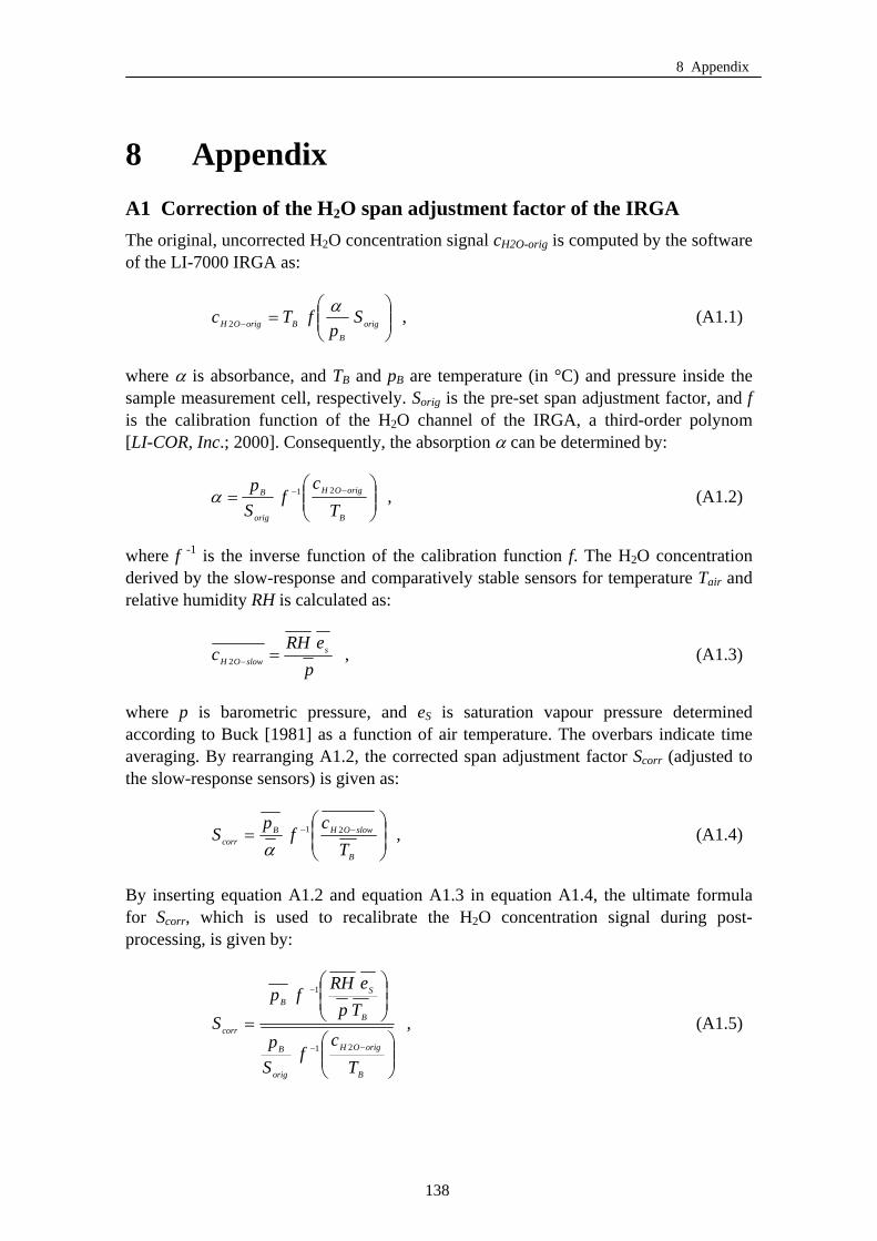
8 Appendix
8 Appendix A1 Correction of the H2O span adjustment factor of the IRGA The original, uncorrected H2O concentration signal cH2O-orig is computed by the software of the LI-7000 IRGA as:
⎟⎟⎠
⎞⎜⎜⎝
⎛=− orig
BBorigOH S
pfTc α
2 , (A1.1)
where α is absorbance, and TB and pB BB are temperature (in °C) and pressure inside the sample measurement cell, respectively. Sorig is the pre-set span adjustment factor, and f is the calibration function of the H2O channel of the IRGA, a third-order polynom [LI-COR, Inc.; 2000]. Consequently, the absorption α can be determined by:
⎟⎟⎠
⎞⎜⎜⎝
⎛= −−
B
origOH
orig
B
Tc
fSp 21α , (A1.2)
where f -1 is the inverse function of the calibration function f. The H2O concentration derived by the slow-response and comparatively stable sensors for temperature Tair and relative humidity RH is calculated as:
peRH
c sslowOH =−2 , (A1.3)
where p is barometric pressure, and eS is saturation vapour pressure determined according to Buck [1981] as a function of air temperature. The overbars indicate time averaging. By rearranging A1.2, the corrected span adjustment factor Scorr (adjusted to the slow-response sensors) is given as:
⎟⎟⎠
⎞⎜⎜⎝
⎛= −−
B
slowOHBcorr T
cf
pS 21
α , (A1.4)
By inserting equation A1.2 and equation A1.3 in equation A1.4, the ultimate formula for Scorr, which is used to recalibrate the H2O concentration signal during post-processing, is given by:
⎟⎟⎠
⎞⎜⎜⎝
⎛
⎟⎟⎠
⎞⎜⎜⎝
⎛
=−−
−
B
origOH
orig
B
B
SB
corr
Tc
fSp
TpeRH
fpS
21
1
, (A1.5)
138
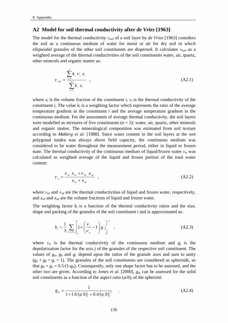
8 Appendix
A2 Model for soil thermal conductivity after de Vries [1963] The model for the thermal conductivity νsoil of a soil layer by de Vries [1963] considers the soil as a continuous medium of water for moist or air for dry soil in which ellipsoidal granules of the other soil constituents are dispersed. It calculates νsoil as a weighted average of the thermal conductivities of the soil constituents water, air, quartz, other minerals and organic matter as:
∑
∑
=
== n
iii
i
n
iii
soil
xk
xk
1
1
νν , (A2.1)
where xi is the volume fraction of the constituent i, νi is the thermal conductivity of the constituent i, The value ki is a weighting factor which represents the ratio of the average temperature gradient in the constituent i and the average temperature gradient in the continuous medium. For the assessment of average thermal conductivity, the soil layers were modelled as mixtures of five constituents (n = 5): water, air, quartz, other minerals and organic matter. The mineralogical composition was estimated from soil texture according to Møberg et al. [1988]. Since water content in the soil layers at the wet polygonal tundra was always above field capacity, the continuous medium was considered to be water throughout the measurement period, either in liquid or frozen state. The thermal conductivity of the continuous medium of liquid/frozen water νw was calculated as weighted average of the liquid and frozen portion of the total water content:
wfwl
wfwfwlwlw xx
xx+
+=
ννν , (A2.2)
where νwl and νwf are the thermal conductivities of liquid and frozen water, respectively, and xwl and xwf are the volume fractions of liquid and frozen water.
The weighting factor ki is a function of the thermal conductivity ratios and the size, shape and packing of the granules of the soil constituent i and is approximated as:
∑=
−
⎥⎦
⎤⎢⎣
⎡⎟⎟⎠
⎞⎜⎜⎝
⎛−+=
cbajj
w
ii gk
,,
1
1131
νν
, (A2.3)
where νw is the thermal conductivity of the continuous medium and gj is the depolarization factor for the axis j of the granules of the respective soil constituent. The values of ga, gb and gc depend upon the ratios of the granule axes and sum to unity (ga + gb + gc = 1). The granules of the soil constituents are considered as spheroids, so that gb = gc = 0.5·(1-ga). Consequently, only one shape factor has to be assessed, and the other two are given. According to Jones et al. [2000], gai can be assessed for the solid soil constituents as a function of the aspect ratio (a/b)i of the spheroid:
( ) ( ) 24.06.111
ii
ai babag
++= . (A2.4)
139
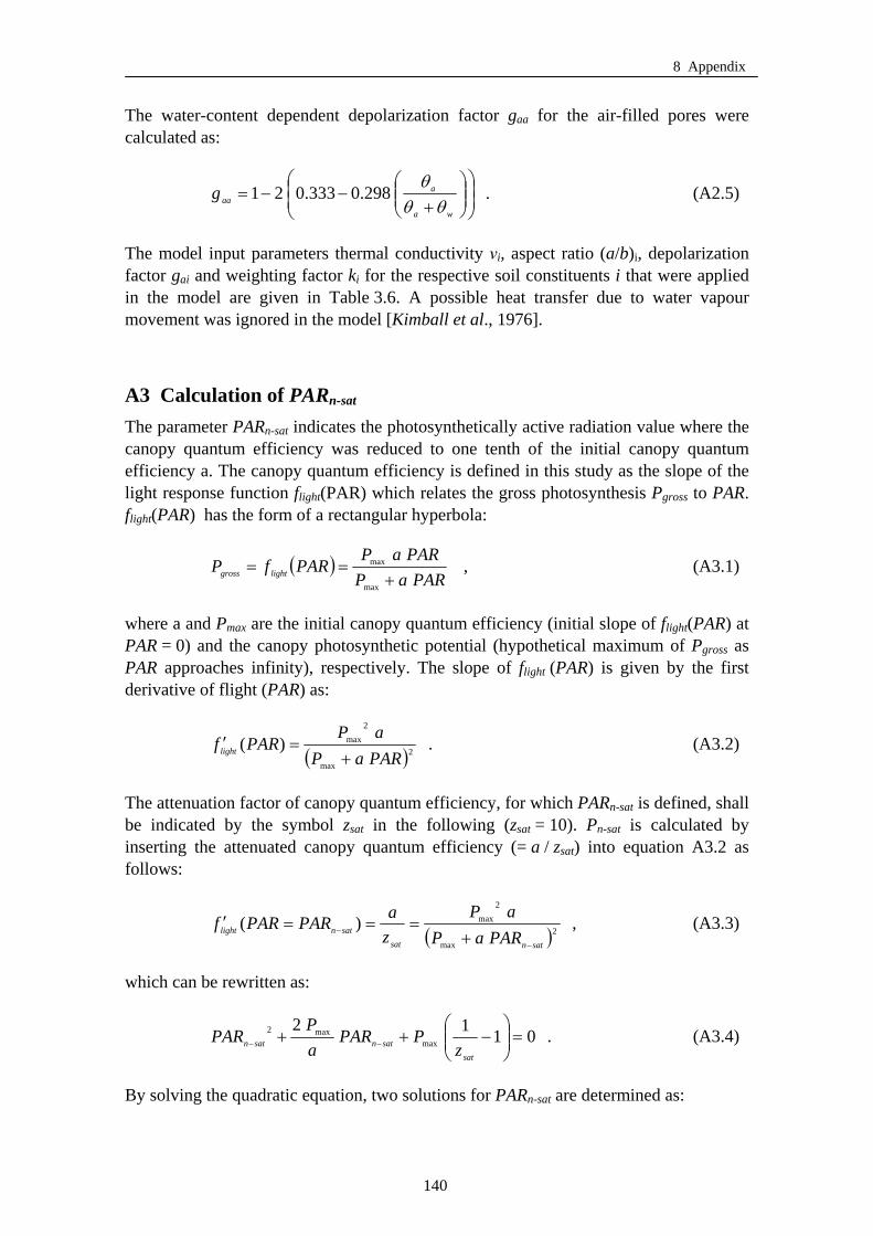
8 Appendix
The water-content dependent depolarization factor gaa for the air-filled pores were calculated as:
⎟⎟⎠
⎞⎜⎜⎝
⎛⎟⎟⎠
⎞⎜⎜⎝
⎛+
−−=wa
aaag
θθθ
298.0333.021 . (A2.5)
The model input parameters thermal conductivity νi, aspect ratio (a/b)i, depolarization factor gai and weighting factor ki for the respective soil constituents i that were applied in the model are given in Table 3.6. A possible heat transfer due to water vapour movement was ignored in the model [Kimball et al., 1976].
A3 Calculation of PARn-sat
The parameter PARn-sat indicates the photosynthetically active radiation value where the canopy quantum efficiency was reduced to one tenth of the initial canopy quantum efficiency a. The canopy quantum efficiency is defined in this study as the slope of the light response function flight(PAR) which relates the gross photosynthesis Pgross to PAR. flight(PAR) has the form of a rectangular hyperbola:
( )PARaP
PARaPPARfP lightgross +
==max
max , (A3.1)
where a and Pmax are the initial canopy quantum efficiency (initial slope of flight(PAR) at PAR = 0) and the canopy photosynthetic potential (hypothetical maximum of Pgross as PAR approaches infinity), respectively. The slope of flight (PAR) is given by the first derivative of flight (PAR) as:
( )2max
2max)(
PARaPaP
PARflight +=′ . (A3.2)
The attenuation factor of canopy quantum efficiency, for which PARn-sat is defined, shall be indicated by the symbol zsat in the following (zsat = 10). Pn-sat is calculated by inserting the attenuated canopy quantum efficiency (= a / zsat) into equation A3.2 as follows:
( )2max
2max)(
satnsatsatnlight PARaP
aPzaPARPARf
−
− +===′ , (A3.3)
which can be rewritten as:
0112max
max2 =⎟⎟⎠
⎞⎜⎜⎝
⎛−++ −−
satsatnsatn z
PPARaP
PAR . (A3.4)
By solving the quadratic equation, two solutions for PARn-sat are determined as:
140

8 Appendix
2
144
2
2max2
2max
max2,1
⎟⎠⎞
⎜⎝⎛ −
−±=−
az
Pa
P
aP
PAR
sat
satn . (A3.5)
Only one solution results in a positive, realistic value for PARn-sat:
2
144
2
2max2
2max
max
⎟⎠⎞
⎜⎝⎛ −
−+=−
az
Pa
P
aP
PAR
sat
satn . (A3.6)
141