Embed Size (px)
Citation preview
DOI: 10.1007/s00224-005-1261-z
Theory Comput. Systems 39, 121–136 (2006) Theory ofComputing
Systems© 2005 Springer Science+Business Media, Inc.
The Expected Competitive Ratio for Weighted CompletionTime Scheduling
Alexander Souza and Angelika Steger
Institute of Theoretical Computer Science, ETH Zurich,Universitatstr. 6, CH-8092 Zurich, Switzerland{steger,asouza}@inf.ethz.ch
Abstract. A set of n independent jobs is to be scheduled without preemptionon m identical parallel machines. For each job j , a diffuse adversary chooses thedistribution Fj of the random processing time Pj from a certain class of distributionsFj . The scheduler is given the expectation µj = E[Pj ], but the actual duration isnot known in advance. A positive weight wj is associated with each job j and alljobs are ready for execution at time zero. The scheduler determines a list of the jobs,which is then scheduled in a non-preemptive manner. The objective is to minimisethe total weighted completion time
∑j wj Cj . The performance of an algorithm is
measured with respect to the expected competitive ratio maxF∈F E[∑
j wj Cj/OPT],where Cj denotes the completion time of job j and OPT the offline optimum value.
We show a general bound on the expected competitive ratio for list schedulingalgorithms, which holds for a class of so-called new-better-than-used processingtime distributions. This class includes, among others, the exponential distribution.
As a special case, we consider the popular rule weighted shortest expectedprocessing time first (WSEPT) in which jobs are processed according to the non-decreasing µj/wj ratio. We show that it achieves E[WSEPT/OPT] ≤ 3 − 1/m forexponential distributed processing times.
1. Introduction
Scheduling problems are very well studied combinatorial optimisation problems. Amongothers, the following completion time scheduling problem and its variants have attractedmuch attention. A set of jobs is to be processed on a set of machines. The objectivefunction is to minimise the total weighed completion time
∑j wj Cj , where Cj denotes
the time when job j is finished and wj denotes a weight associated with job j .
122 A. Souza and A. Steger
In this paper we consider the expected competitive ratio of scheduling algorithmsfor stochastic variants of the problem. This measure is defined as the expectation (takenover all instances) of the objective-value achieved by an algorithm on a certain instancerelated to the optimum value of the same instance. One property of this measure is thatit favours algorithms that perform well on “many” instances.
Previous Work. The deterministic version of the completion time scheduling problemhas been studied intensively since the 1950s. For the weighted single-machine problemSmith [27] proved optimality of the so-called weighted shortest processing time first(WSPT) rule: schedule the jobs in order of the non-decreasing processing time andweight ratio. For the unweighted problem, i.e., all weights are equal to one, with midentical parallel machines, the optimality of the shortest processing time first (SPT)strategy was shown by Conway et al. [5].
In contrast, Bruno and Sethi [2] showed that the weighted problem with m parallelmachines is alreadyNP-hard in the ordinary sense for constant m. However, Sahni [22]proved that it admits a fully polynomial time approximation scheme (FPTAS). If thenumber of machines is considered as part of the input, Lageweg and Lenstra [14] estab-lished that the weighted problem isNP-hard in the strong sense (see also problem SS13of [7]). An exact algorithm was given by Sahni [22]. Skutella and Woeginger [26] found apolynomial time approximation scheme (PTAS). Kawaguchi and Kyan [12] establishedthat WSPT achieves 1
2 (1+√
2) approximation ratio. Besides that, several constant factorapproximations are known for variants of the problem, see, e.g., [16], [17], [24], [10],and [25].
Evidently, this problem was studied extensively from the worst-case perspective.However, a drawback of this approach is that it may be overly pessimistic: a schedulingalgorithm with bad worst-case behaviour may perform rather well in practical appli-cations. A natural step to overcome this problem is to consider stochastic scheduling,i.e., to interpret input data as random variables and to measure the performance of analgorithm ALG by its expected objective-value E[ALG].
In stochastic completion time scheduling, the scheduler is given the weight andexpected processing time for each job and the objective function is to minimise theexpected total weighted completion time E[
∑j wj Cj ]. Hence, an algorithm MIN is con-
sidered optimal with respect to that measure if it minimises the expected total weightedcompletion time over all algorithms.
Models that areNP-hard in a deterministic setting sometimes allow a simple priorityrule to be optimal for the probabilistic counterpart. For example, the rule shortest expectedprocessing time first (SEPT), i.e., schedule jobs in order of non-decreasing expectedprocessing times, is known to be optimal for many variants, see, e.g., [21], [29], [3],[11], and [28]. Moreover, for the weighted single-machine problem, the rule weightedshortest expected processing time first (WSEPT) is optimal [18]. WSEPT schedules thejobs in non-decreasing order of the expected processing time over weight ratio.
In their work Mohring et al. [15] proved very general bounds on LP-based algorithmsfor many stochastic completion time scheduling problems. Their method is based on LP-relaxations of a deterministic problem, where an optimum solution to this LP yields alower bound for E[MIN]. In addition, this solution also yields a priority rule which canbe shown to be only a constant factor larger than E[MIN] (with mild assumptions onprocessing time distributions). Also additional constraints, e.g., release dates can be
Competitive Ratio for Weighted Completion Time Scheduling 123
handled with minor modifications to the LP. One of the main results is that for m parallelmachines,
E[WSEPT]
E[MIN]≤ 2− 1
m
holds if processing times are drawn from distributions that are new-better-than-used inexpectation (NBUE).
One property of the performance measure E[ALG] is that instances x with smallvalue ALG(x) tend to be neglected since they contribute little to the overall expectedvalue. Hence, in this measure, algorithms are preferred that perform well on instancesx with large optimum value OPT(x). It depends on the application if such behaviour isdesireable, but if one is interested in algorithms that perform well on “many” instances,this measure may seem inappropriate.
Let ALG(x) denote the objective-value achieved by a certain algorithm and let OPT(x)be the optimum value on instance x , then E[ALG/OPT] defines the expected competitiveratio, where the expectation is taken over all instances.
Regarding the above drawback, the measure E[ALG/OPT] seems to be interestingfor the following intuition. The ratio ALG(x)/OPT(x) relates the value of the objectivefunction achieved by some algorithm ALG to the optimum OPT on the instance x . Thus,the algorithm is considered to perform well on instances that yield a small ratio, and badon instances with a large ratio. Hence, if for “most” instances a small ratio is attained,the “few” instances with a large ratio will not increase the expectation drastically. Seealso [23] for a discussion.
Despite the vast literature on stochastic scheduling problems, it seems that theexpected competitive ratio has only been considered in a paper by Coffman and Gilbert[4] and in the recent work of Scharbrodt et al. [23].
In [23] the unweighted completion time problem on parallel machines is consideredfor the SEPT rule. The main result is that the SEPT algorithm yields
E
[SEPT
OPT
]= O(1)
for identical parallel machines under relatively weak assumptions on job processing timedistributions. Here SEPT denotes the objective-value achieved by the SEPT algorithm andOPT the objective-value of an optimum offline algorithm, i.e., an algorithm that is giventhe actual realisations of processing times. The general approach is to partition theprobability space according to a series of “bad events”. These events yield a series ofbounds that give an estimate for the probability of “larger” values of SEPT/OPT.
In this paper we consider the weighted version of the completion time schedulingproblem, prove a general bound on the expected competitive ratio, and analyse theWSEPT algorithm.
Model, Problem Definition, and Notation. Consider a set J = {1, 2, . . . , n} of n inde-pendent jobs that have to be scheduled non-preemptively on a set M = {1, 2, . . . ,m} ofm identical parallel machines. For each job j , a so-called diffuse adversary (see [13])chooses the distribution Fj of the random processing time Pj ≥ 0 out of a certain classof distributions Fj . We assume that the processing times Pj are stochastically indepen-dent. The scheduler is given the expectation µj = E[Pj ] of each job j , but the actual
124 A. Souza and A. Steger
realisation pj is only learned upon job completion. A positive weight wj is associatedwith each job j ∈ J and all jobs are ready for execution at time zero. Every machinecan process at most one job at a time. Each job can be executed by any of the machines,but preemption and delays are not permitted. The completion time Cj of a job j ∈ J isthe latest point in time, such that a machine is busy processing the job.
In list scheduling, jobs are processed one-by-one according to a priority list. A so-called online list scheduling algorithm is given weight wj and mean µj for all j ∈ Jand, based on that information, deterministically constructs a permutation π of J . Thislist π is then scheduled according to the following policy: whenever a machine is idleand the list is not empty, the job at the head of the list is removed and processed non-preemptively and without delay on the idle machine (with least index). Notice that theactual realisations of processing times are learned only upon job completion, i.e., thelist is constructed offline, while the schedule is constructed online.
Once a realisation p = (p1, p2, . . . , pn) of job processing times is fixed, this policyyields a realisation of the random variable TWC(π) = ∑
j∈J wj Cj , which denotes thetotal weighted completion time for list π . Thus, for any realisation of job processingtimes, an offline optimum list π∗ is defined by
OPT(p) = TWC(π∗) = min{TWC(π): π is a permutation of J }. (1)
This yields the random variable OPT of the minimum value of the objective function for therandom processing time vector P = (P1, P2, . . . , Pn). Let ALG be an online list schedul-ing algorithm and let π denote the list produced by ALG on inputµ = (µ1, µ2, . . . , µn)
and w = (w1, w2, . . . , wn). We define the random variable ALG = TWC(π) as the totalweighted completion time achieved by the algorithm ALG. It is important to note thatany online list scheduling algorithm deterministically constructs one fixed list for allrealisations, while the optimum list may be different for each realisation.
For any algorithm ALG, the ratio ALG/OPT defines a random variable that measuresthe relative performance of that algorithm compared with the offline optimum. We maythus define the expected competitive ratio of an algorithm ALG by
R(ALG,F) = max
{E
[ALG
OPT
]: F ∈ F
},
where the job processing time distributions F = (F1, F2, . . . , Fn) are chosen by adiffuse adversary from a class of distributions F = (F1,F2, . . . ,Fn). The objective isto minimise the expected competitive ratio, and thus an algorithm is called competitiveoptimal if it yields this minimum over all algorithms.
In the standard classification scheme by Graham et al. [9] our completion timescheduling problem is denoted
P | Pj ∼ Fj (µj ) ∈ Fj |∑
j
wj Cj .
The performance of an algorithm is measured in terms of expected competitive ratioR(ALG,F).
This model can be seen as a hybrid between stochastic scheduling models andcompetitive analysis, since it comprises important aspects of them both.
Competitive Ratio for Weighted Completion Time Scheduling 125
In competitive analysis (see [1] for an introduction) the input for an algorithmbecomes available only gradually and usually driven by an adversary. The competitiveratio is defined by the objective-value of a certain algorithm on a worst-case inputcompared with the offline-optimum, i.e., an optimum algorithm that sees the wholeinput in advance. An unrestricted adversary is usually considered overly powerful. Oneapproach to limit its power is the diffuse adversary model introduced by Koutsoupiasand Papadimitriou [13], where the adversary is allowed to choose the distribution ofthe input out of a certain class of distributions. As is done in competitive analysis, ourmodel relates the performance of an algorithm to the offline optimum on each instance.However, rather than taking the maximum value of that ratio, we take the average overall instances weighted with a distribution specified by a diffuse adversary.
The similarities to classical stochastic scheduling are that processing times are drawnfrom a probability distribution, and that the number n of jobs, their weights w and mostimportantly their expected durations µ are known. The most important difference is thatin stochastic scheduling the optimum is usually not defined as the offline optimum, but asan algorithm that, givenw andµ only, minimises the expected total weighted completiontime.
Results. We introduce the class of distributions that are new-better-than-used in expec-tation relative to a function h (NBUEh). The NBUEOPT class comprises the exponential,geometric, and uniform distribution.
We allow the adversary to choose NBUEOPT processing time distributions and derivebounds to online list scheduling algorithms for the problem
P | Pj ∼ F(µj ) ∈ NBUEOPT |∑
j
wj Cj ,
where the performance of an algorithm is measured in terms of expected competitiveratio R(ALG,NBUEOPT).
Our analysis depends on a quantity α which is an upper bound of the probabilitythat any pair of jobs is in the wrong order in a list of a certain online list algorithm ALG,compared with an optimum list. We would also like to point out that our analysis issignificantly simpler compared with [23].
Theorem 3.2 states that R(ALG,NBUEOPT) ≤ 1/(1− α) holds for the single-machine case. In Corollary 3.7 we show that R(ALG,NBUEOPT) ≤ 1/(1− α)+1−1/mholds for m identical parallel machines.
These results reflect well the intuition that an algorithm should perform better, thesmaller its probability of sequencing jobs in the wrong order.
As an important special case, Corollary 3.8 yields E[WSEPT/OPT] ≤ 3 − 1/m forthe WSEPT algorithm with m identical parallel machines and exponential distributedprocessing times. Simulations empirically demonstrate tightness of this bound.
2. New-Better-Than-Used Distributions
In this section we define a class of processing time distributions from which the dif-fuse adversary is allowed to choose. However, we first discuss the class of distributions
126 A. Souza and A. Steger
that are new-better-than-used in expectation (NBUE). The concept of NBUE randomvariables is well known in reliability theory [8], where it is considered as a relativelyweak assumption. NBUE distributions are typically used to model the aging of systemcomponents, but have also proved useful in the context of stochastic scheduling. For theproblem P |√Var[Pj ] ≤ E[Pj ] |E[
∑j wj Cj ] the bound E[WSEPT] ≤ (2− 1/m)E[MIN]
of Mohring et al. [15] holds for NBUE processing time distributions as an important spe-cial case. In addition, Pinedo and Weber [19] give bounds for shop scheduling problemsassuming NBUE processing time distributions.
A random variable X ≥ 0 is NBUE if E[X − t | X ≥ t] ≤ E[X ] holds for allt ≥ 0, see, e.g., [8]. Examples of NBUE distributions are uniform, exponential, Erlang,geometric, and Weibull distribution (with shape parameter at least one).
Let X denote a random variable taking values in a set V ⊂ R+0 and let h(x) > 0 be areal-valued function defined on V . The random variable X ≥ 0 is new-better-than-usedin expectation relative to h (NBUEh) if
E
[X − t
h(X)
∣∣∣∣ X ≥ t
]≤ E
[X
h(X)
](2)
holds for all t ∈ V , provided these expectations exist.It is natural to extend the concept of NBUEh distributions to functions h that have
more than one variable. Let X denote a random variable taking values in a set V ⊂ R+0 ,let y ∈ W ⊂ Rk for k ∈ N, and let h(x, y) > 0 be a real-valued function defined on(V,W ). The random variable X ≥ 0 is NBUEh if
E
[X − t
h(X, y)
∣∣∣∣ X ≥ t
]≤ E
[X
h(X, y)
](3)
holds for all t ∈ V and all y ∈ W , provided these expectations exist.In what follows, the distribution function of a random variable X , is denoted by
FX (t) = Pr[X ≤ t] and let fX (t) = (d/dt)FX (t) denote its density. For any event A, letFX |A(t) = Pr[X ≤ t | A] and fX |A(t) = (d/dt)FX |A(t) be the conditional distribution,and the conditional density of X given A, respectively. Now we establish several generalproperties of NBUEh distributions.
Lemma 2.1. Let X be NBUEh and let Y be a random vector taking values in Windependently of X , then
E
[X − t
h(X, Y )
∣∣∣∣ X ≥ t
]≤ E
[X
h(X, Y )
].
Proof. Since X is NBUEh (3) yields
E
[X − t
h(X, Y )
∣∣∣∣ X ≥ t
]=∫
y∈WE
[X − t
h(X, y)
∣∣∣∣ X ≥ t
]fY (y) dy
≤∫
y∈WE
[X
h(X, y)
]fY (y)dy = E
[X
h(X, Y )
],
which completes the proof.
Competitive Ratio for Weighted Completion Time Scheduling 127
Lemma 2.2. Let X be NBUEh , α > 0, and let Y be a random vector taking values inW independently of X , then
E
[αX − t
h(X, Y )
∣∣∣∣ αX ≥ t
]≤ E
[αX
h(X, Y )
]
holds for all t ∈ V .
Proof. Let y ∈ W be fixed. As X is NBUEh one obtains that
E
[αX − t
h(X, y)
∣∣∣∣ αX ≥ t
]= αE
[X − t/α
h(X, y)
∣∣∣∣ X ≥ t
α
]
≤ αE[
X
h(X, y)
]= E
[αX
h(X, y)
]
for all t ≥ 0. Taking the expectation of Y as in Lemma 2.1 completes the proof.
Lemma 2.3. Let X be NBUEh , let Y be a random vector taking values in W indepen-dently of X , and let g(y) be a function defined on W taking values in V , then
E
[X − g(Y )
h(X, Y )
∣∣∣∣ X ≥ g(Y )
]≤ E
[X
h(X, Y )
].
Proof. Since (3) holds for all t ∈ V it holds especially for t = g(y). Repeating theproof of Lemma 2.1 with this choice yields the claim.
The next lemmas show that exponential, geometric, and uniform distributed randomvariables are NBUEh if h is a non-decreasing function in x , i.e., h(x + t, y) ≥ h(x, y)for all x, y and t ≥ 0. We use X ∼ Uni(a, b), X ∼ Exp(λ), and X ∼ Geo(p) todenote that the distribution of the random variable X is uniform in [a, b], exponentialwith parameter λ, and geometric with probability p, respectively.
Lemma 2.4. If X ∼ Exp(λ) and h(x, y) > 0 is non-decreasing in x , then X is NBUEh .
Proof. For all s ≥ 0 we have fX |X≥t (t + s) = fX (s) since X has memoryless densityfX . As h is non-decreasing in x it holds that h(t+s, y) ≥ h(s, y) for t ≥ 0. We thereforeobtain
E
[X − t
h(X, y)
∣∣∣∣ X ≥ t
]=∫ ∞
x=t
x − t
h(x, y)fX |X≥t (x) dx
=∫ ∞
s=0
t + s − t
h(t + s, y)fX |X≥t (t + s) ds
≤∫ ∞
s=0
s
h(s, y)fX (s) ds = E
[X
h(X, y)
],
which proves the lemma.
128 A. Souza and A. Steger
Lemma 2.5. If X ∼ Geo(p) and h(x, y) > 0 is non-decreasing in x , then X is NBUEh .
Proof. The proof for the exponential distribution analogously carries over to the geo-metric distribution.
Lemma 2.6. If X ∼ Uni(a, b) where 0 ≤ a < b and h(x, y) > 0 is non-decreasingin x , then X is NBUEh .
Proof. We want to show that
E
[X − t
h(X, y)
∣∣∣∣ X ≥ t
]≤ E
[X
h(X, y)
]
for all t ∈ V = [a, b) and y ∈ W . Let the random variable T ∼ Uni(a, b) be independentof X . Let t ∈ [a, b) be arbitrary but fixed, and introduce the (dependent) random variableS = ((b − t)/(b − a))(T − a) with distribution S ∼ Uni(0, b − t). Observe that fort ≤ x ≤ b we have Pr[X ≤ x | X ≥ t] = (x − t)/(b − t) = Pr[S ≤ x − t] and thusfX |X≥t (x) = 1/(b − t) = fS(x − t). Therefore
E
[X − t
h(X, y)
∣∣∣∣ X ≥ t
]=∫ b
x=t
x − t
h(x, y)
1
b − tdx
=∫ b−t
s=0
s
h(s + t, y)
1
b − tds = E
[S
h(S + t, y)
].
With a ≥ 0 and (b − t)/(b − a) ≤ 1 we have S ≤ T . A simple calculation shows thatsince T < b and a ≤ t we have T ≤ ((b − t)/(b − a))(T − a) + t = S + t . Hence,since h is non-decreasing we find h(S + t, y) ≥ h(T, y) > 0 and we have
E
[S
h(S + t, y)
]≤ E
[T
h(T, y)
]= E
[X
h(X, y)
],
which completes the proof since X and T are identically distributed.
3. Weighted Completion Time Scheduling
Recall that the random variable OPT measures the value of the offline optimum of ourproblem. If we interpret OPT as a real-valued function defined on the set of processingtime vectors, then NBUEOPT induces a class of distributions. In particular, we allow thediffuse adversary to choose NBUEOPT processing time distributions in the followingway: all jobs fall into the same class, e.g., they are all exponential distributed, but theparameter, and thus the mean µj of each individual job j , is arbitrary. We denote thisdegree of freedom by Pj ∼ F(µj ) ∈ NBUEOPT. Hence we consider the problem
P | Pj ∼ F(µj ) ∈ NBUEOPT |∑
j
wj Cj
Competitive Ratio for Weighted Completion Time Scheduling 129
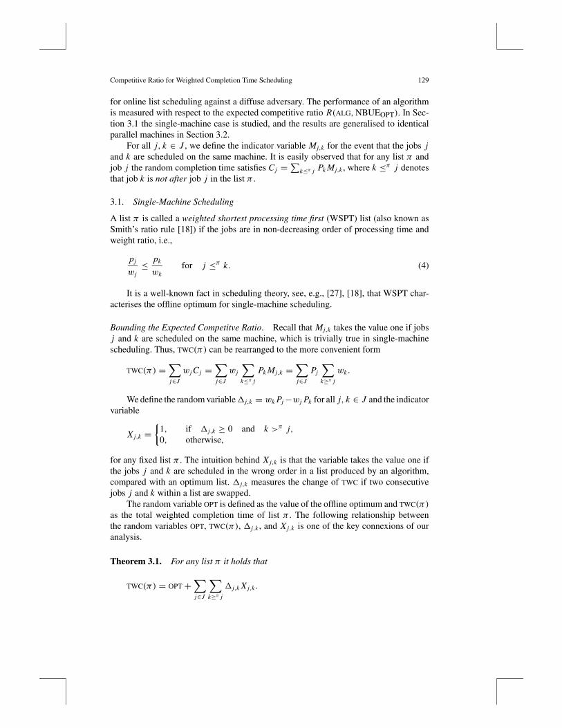
for online list scheduling against a diffuse adversary. The performance of an algorithmis measured with respect to the expected competitive ratio R(ALG,NBUEOPT). In Sec-tion 3.1 the single-machine case is studied, and the results are generalised to identicalparallel machines in Section 3.2.
For all j, k ∈ J , we define the indicator variable Mj,k for the event that the jobs jand k are scheduled on the same machine. It is easily observed that for any list π andjob j the random completion time satisfies Cj =
∑k≤π j Pk Mj,k , where k ≤π j denotes
that job k is not after job j in the list π .
3.1. Single-Machine Scheduling
A list π is called a weighted shortest processing time first (WSPT) list (also known asSmith’s ratio rule [18]) if the jobs are in non-decreasing order of processing time andweight ratio, i.e.,
pj
wj≤ pk
wkfor j ≤π k. (4)
It is a well-known fact in scheduling theory, see, e.g., [27], [18], that WSPT char-acterises the offline optimum for single-machine scheduling.
Bounding the Expected Competitve Ratio. Recall that Mj,k takes the value one if jobsj and k are scheduled on the same machine, which is trivially true in single-machinescheduling. Thus, TWC(π) can be rearranged to the more convenient form
TWC(π) =∑j∈J
wj Cj =∑j∈J
wj
∑k≤π j
Pk Mj,k =∑j∈J
Pj
∑k≥π j
wk .
We define the random variable j,k = wk Pj−wj Pk for all j, k ∈ J and the indicatorvariable
X j,k ={
1, if j,k ≥ 0 and k >π j,0, otherwise,
for any fixed list π . The intuition behind X j,k is that the variable takes the value one ifthe jobs j and k are scheduled in the wrong order in a list produced by an algorithm,compared with an optimum list. j,k measures the change of TWC if two consecutivejobs j and k within a list are swapped.
The random variable OPT is defined as the value of the offline optimum and TWC(π)
as the total weighted completion time of list π . The following relationship betweenthe random variables OPT, TWC(π), j,k , and X j,k is one of the key connexions of ouranalysis.
Theorem 3.1. For any list π it holds that
TWC(π) = OPT+∑j∈J
∑k≥π j
j,k X j,k .
130 A. Souza and A. Steger
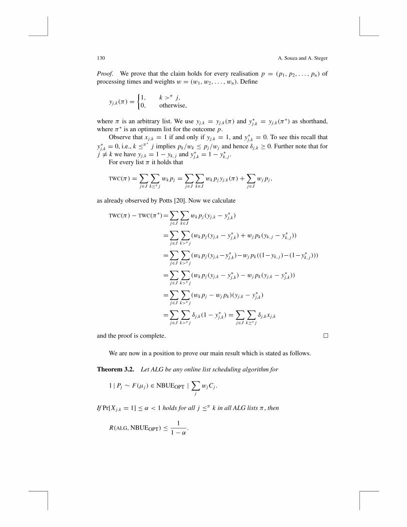
Proof. We prove that the claim holds for every realisation p = (p1, p2, . . . , pn) ofprocessing times and weights w = (w1, w2, . . . , wn). Define
yj,k(π) ={
1, k >π j,0, otherwise,
where π is an arbitrary list. We use yj,k = yj,k(π) and y∗j,k = yj,k(π∗) as shorthand,
where π∗ is an optimum list for the outcome p.Observe that xj,k = 1 if and only if yj,k = 1, and y∗j,k = 0. To see this recall that
y∗j,k = 0, i.e., k ≤π∗ j implies pk/wk ≤ pj/wj and hence δj,k ≥ 0. Further note that forj �= k we have yj,k = 1− yk, j and y∗j,k = 1− y∗k, j .
For every list π it holds that
TWC(π) =∑j∈J
∑k≥π j
wk pj =∑j∈J
∑k∈J
wk pj yj,k(π)+∑j∈J
wj pj ,
as already observed by Potts [20]. Now we calculate
TWC(π)− TWC(π∗)=∑j∈J
∑k∈J
wk pj (yj,k − y∗j,k)
=∑j∈J
∑k>π j
(wk pj (yj,k − y∗j,k)+ wj pk(yk, j − y∗k, j ))
=∑j∈J
∑k>π j
(wk pj (yj,k−y∗j,k)−wj pk((1−yk, j )−(1−y∗k, j )))
=∑j∈J
∑k>π j
(wk pj (yj,k − y∗j,k)− wj pk(yj,k − y∗j,k))
=∑j∈J
∑k>π j
(wk pj − wj pk)(yj,k − y∗j,k)
=∑j∈J
∑k>π j
δj,k(1− y∗j,k) =∑j∈J
∑k≥π j
δj,k xj,k
and the proof is complete.
We are now in a position to prove our main result which is stated as follows.
Theorem 3.2. Let ALG be any online list scheduling algorithm for
1 | Pj ∼ F(µj ) ∈ NBUEOPT |∑
j
wj Cj .
If Pr[X j,k = 1] ≤ α < 1 holds for all j ≤π k in all ALG lists π , then
R(ALG,NBUEOPT) ≤ 1
1− α .
Competitive Ratio for Weighted Completion Time Scheduling 131
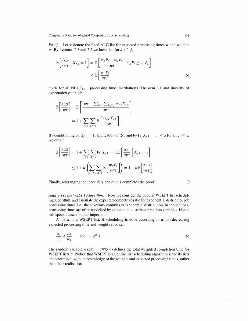
Proof. Let π denote the fixed ALG list for expected processing times µ and weightsw. By Lemmas 2.3 and 2.2 we have that for k >π j ,
E
[ j,k
OPT
∣∣∣∣ X j,k = 1
]= E
[wk Pj − wj Pk
OPT
∣∣∣∣ wk Pj ≥ wj Pk
]
≤ E[wk Pj
OPT
](5)
holds for all NBUEOPT processing time distributions. Theorem 3.1 and linearity ofexpectation establish
E
[ALG
OPT
]= E
[OPT+∑j∈J
∑k≥π j j,k X j,k
OPT
]
= 1+∑j∈J
∑k≥π j
E
[ j,k X j,k
OPT
].
By conditioning on X j,k = 1, application of (5), and by Pr[X j,k = 1] ≤ α for all j ≤π kwe obtain
E
[ALG
OPT
]= 1+
∑j∈J
∑k≥π j
Pr[X j,k = 1]E
[ j,k
OPT
∣∣∣∣ X j,k = 1
]
≤ 1+ α(∑
j∈J
∑k≥π j
E
[wk Pj
OPT
])= 1+ αE
[ALG
OPT
].
Finally, rearranging the inequality and α < 1 completes the proof.
Analysis of the WSEPT Algorithm. Now we consider the popular WSEPT list schedul-ing algorithm, and calculate the expected competitve ratio for exponential distributed jobprocessing times, i.e., the adversary commits to exponential distribution. In applications,processing times are often modelled by exponential distributed random variables. Hencethis special case is rather important.
A list π is a WSEPT list, if scheduling is done according to a non-decreasingexpected processing time and weight ratio, i.e.,
µj
wj≤ µk
wkfor j ≤π k. (6)
The random variable WSEPT = TWC(π) defines the total weighted completion time forWSEPT lists π . Notice that WSEPT is an online list scheduling algorithm since its listsare determined with the knowledge of the weights and expected processing times, ratherthan their realisations.
132 A. Souza and A. Steger
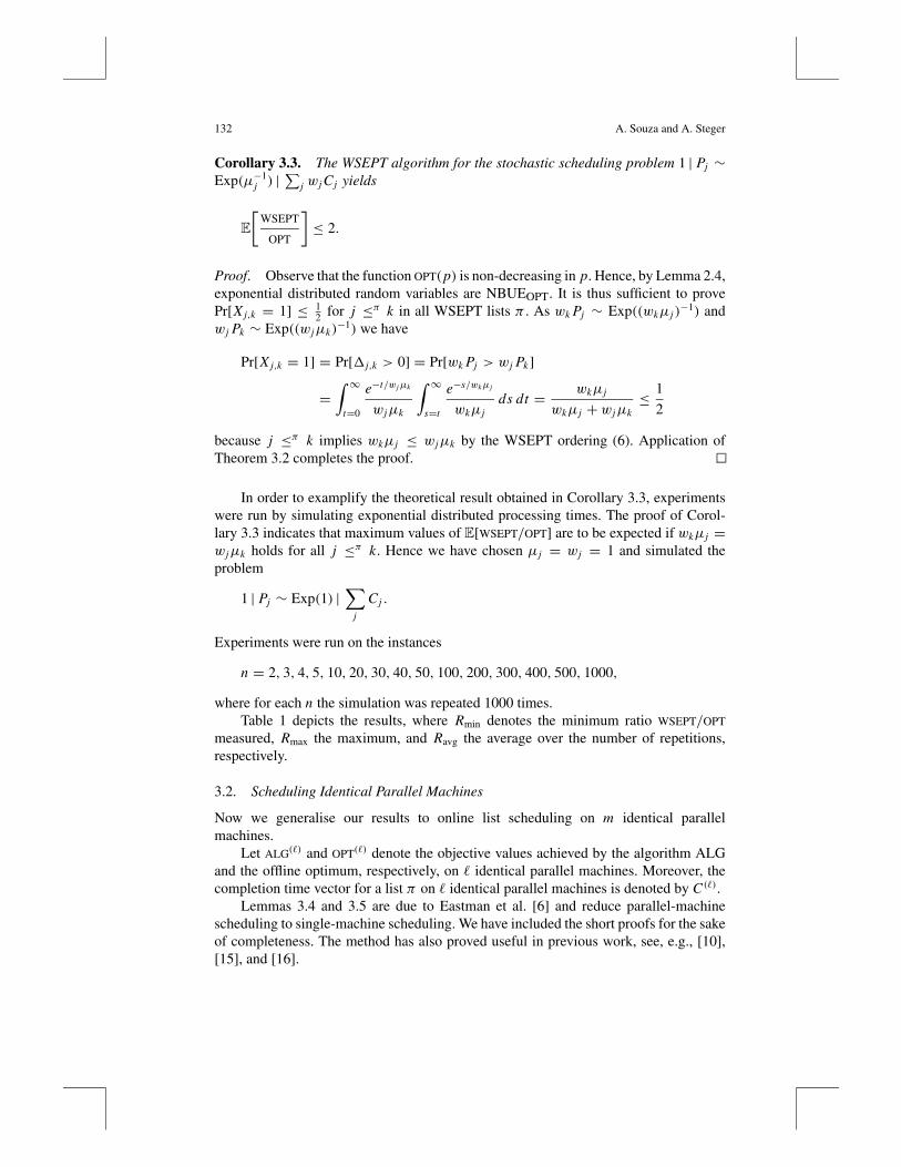
Corollary 3.3. The WSEPT algorithm for the stochastic scheduling problem 1 | Pj ∼Exp(µ−1
j ) |∑
j wj Cj yields
E
[WSEPT
OPT
]≤ 2.
Proof. Observe that the function OPT(p) is non-decreasing in p. Hence, by Lemma 2.4,exponential distributed random variables are NBUEOPT. It is thus sufficient to provePr[X j,k = 1] ≤ 1
2 for j ≤π k in all WSEPT lists π . As wk Pj ∼ Exp((wkµj )−1) and
wj Pk ∼ Exp((wjµk)−1) we have
Pr[X j,k = 1] = Pr[ j,k > 0] = Pr[wk Pj > wj Pk]
=∫ ∞
t=0
e−t/wjµk
wjµk
∫ ∞s=t
e−s/wkµj
wkµjds dt = wkµj
wkµj + wjµk≤ 1
2
because j ≤π k implies wkµj ≤ wjµk by the WSEPT ordering (6). Application ofTheorem 3.2 completes the proof.
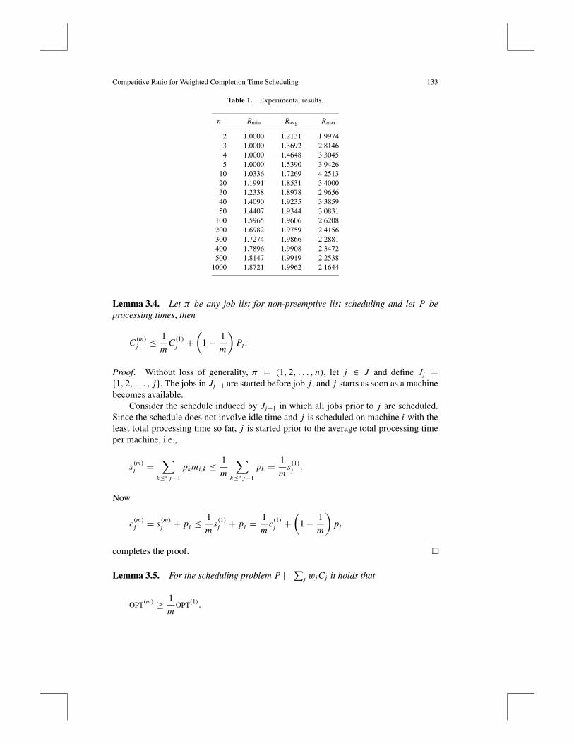
In order to examplify the theoretical result obtained in Corollary 3.3, experimentswere run by simulating exponential distributed processing times. The proof of Corol-lary 3.3 indicates that maximum values of E[WSEPT/OPT] are to be expected if wkµj =wjµk holds for all j ≤π k. Hence we have chosen µj = wj = 1 and simulated theproblem
1 | Pj ∼ Exp(1) |∑
j
Cj .
Experiments were run on the instances
n = 2, 3, 4, 5, 10, 20, 30, 40, 50, 100, 200, 300, 400, 500, 1000,
where for each n the simulation was repeated 1000 times.Table 1 depicts the results, where Rmin denotes the minimum ratio WSEPT/OPT
measured, Rmax the maximum, and Ravg the average over the number of repetitions,respectively.
3.2. Scheduling Identical Parallel Machines
Now we generalise our results to online list scheduling on m identical parallelmachines.
Let ALG(�) and OPT(�) denote the objective values achieved by the algorithm ALGand the offline optimum, respectively, on � identical parallel machines. Moreover, thecompletion time vector for a list π on � identical parallel machines is denoted by C (�).
Lemmas 3.4 and 3.5 are due to Eastman et al. [6] and reduce parallel-machinescheduling to single-machine scheduling. We have included the short proofs for the sakeof completeness. The method has also proved useful in previous work, see, e.g., [10],[15], and [16].
Competitive Ratio for Weighted Completion Time Scheduling 133
Table 1. Experimental results.
n Rmin Ravg Rmax
2 1.0000 1.2131 1.99743 1.0000 1.3692 2.81464 1.0000 1.4648 3.30455 1.0000 1.5390 3.9426
10 1.0336 1.7269 4.251320 1.1991 1.8531 3.400030 1.2338 1.8978 2.965640 1.4090 1.9235 3.385950 1.4407 1.9344 3.0831
100 1.5965 1.9606 2.6208200 1.6982 1.9759 2.4156300 1.7274 1.9866 2.2881400 1.7896 1.9908 2.3472500 1.8147 1.9919 2.2538
1000 1.8721 1.9962 2.1644
Lemma 3.4. Let π be any job list for non-preemptive list scheduling and let P beprocessing times, then
C (m)j ≤ 1
mC (1)
j +(
1− 1
m
)Pj .
Proof. Without loss of generality, π = (1, 2, . . . , n), let j ∈ J and define Jj ={1, 2, . . . , j}. The jobs in Jj−1 are started before job j , and j starts as soon as a machinebecomes available.
Consider the schedule induced by Jj−1 in which all jobs prior to j are scheduled.Since the schedule does not involve idle time and j is scheduled on machine i with theleast total processing time so far, j is started prior to the average total processing timeper machine, i.e.,
s(m)j =∑
k≤π j−1
pkmi,k ≤ 1
m
∑k≤π j−1
pk = 1
ms(1)j .
Now
c(m)j = s(m)j + pj ≤ 1
ms(1)j + pj = 1
mc(1)j +
(1− 1
m
)pj
completes the proof.
Lemma 3.5. For the scheduling problem P | | ∑j wj Cj it holds that
OPT(m) ≥ 1
mOPT(1).
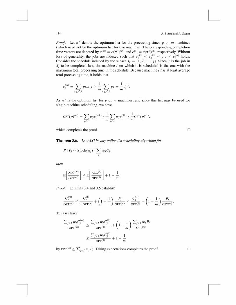
134 A. Souza and A. Steger
Proof. Let π∗ denote the optimum list for the processing times p on m machines(which need not be the optimum list for one machine). The corresponding completiontime vectors are denoted by c(m) = c(π∗)(m) and c(1) = c(π∗)(1), respectively. Withoutloss of generality, the jobs are indexed such that c(m)1 ≤ c(m)2 ≤ . . . ≤ c(m)n holds.Consider the schedule induced by the subset Jj = {1, 2, . . . , j}. Since j is the job inJj to be completed last, the machine i on which it is scheduled is the one with themaximum total processing time in the schedule. Because machine i has at least averagetotal processing time, it holds that
c(m)j =∑
k≤π∗ j
pkmi,k ≥ 1
m
∑k≤π∗ j
pk = 1
mc(1)j .
As π∗ is the optimum list for p on m machines, and since this list may be used forsingle-machine scheduling, we have
OPT(p)(m) =∑j∈J
wj c(m)j ≥
1
m
∑j∈J
wj c(1)j ≥
1
mOPT(p)(1),
which completes the proof.
Theorem 3.6. Let ALG be any online list scheduling algorithm for
P | Pj ∼ Stoch(µj ) |∑
j
wj Cj ,
then
E
[ALG(m)
OPT(m)
]≤ E
[ALG(1)
OPT(1)
]+ 1− 1
m.
Proof. Lemmas 3.4 and 3.5 establish
C (m)j
OPT(m)≤ C (1)
j
mOPT(m)+(
1− 1
m
)Pj
OPT(m)≤ C (1)
j
OPT(1)+(
1− 1
m
)Pj
OPT(m).
Thus we have∑j∈J wj C
(m)j
OPT(m)≤∑
j∈J wj C(1)j
OPT(1)+(
1− 1
m
) ∑j∈J wj Pj
OPT(m)
≤∑
j∈J wj C(1)j
OPT(1)+ 1− 1
m
by OPT(m) ≥∑j∈J wj Pj . Taking expectations completes the proof.
Competitive Ratio for Weighted Completion Time Scheduling 135
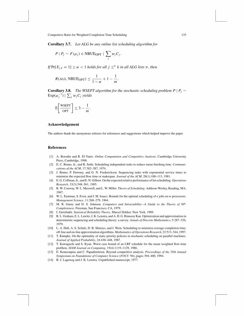
Corollary 3.7. Let ALG be any online list scheduling algorithm for
P | Pj ∼ F(µj ) ∈ NBUEOPT |∑
j
wj Cj .
If Pr[X j,k = 1] ≤ α < 1 holds for all j ≤π k in all ALG lists π , then
R(ALG,NBUEOPT) ≤ 1
1− α + 1− 1
m.
Corollary 3.8. The WSEPT algorithm for the stochastic scheduling problem P | Pj ∼Exp(µ−1
j ) |∑
j wj Cj yields
E
[WSEPT
OPT
]≤ 3− 1
m.
Acknowledgement
The authors thank the anonymous referees for references and suggestions which helped improve the paper.
References
[1] A. Borodin and R. El-Yaniv. Online Computation and Competitive Analysis. Cambridge UniversityPress, Cambridge, 1998.
[2] E. C. Bruno, Jr., and R. Sethi. Scheduling independent tasks to reduce mean finishing time. Communi-cations of the ACM, 17:382–387, 1974.
[3] J. Bruno, P. Downey, and G. N. Frederickson. Sequencing tasks with exponential service times tominimize the expected flow time or makespan. Journal of the ACM, 28(1):100–113, 1981.
[4] E. G. Coffman, Jr., and E. N. Gilbert. On the expected relative performance of list scheduling. OperationsResearch, 33(3):548–561, 1985.
[5] R. W. Conway, W. L. Maxwell, and L. W. Miller. Theory of Scheduling. Addison-Wesley, Reading, MA,1967.
[6] W. L. Eastman, S. Even, and I. M. Isaacs. Bounds for the optimal scheduling of n jobs on m processors.Management Science, 11:268–279, 1964.
[7] M. R. Garey and D. S. Johnson. Computers and Intractability—A Guide to the Theory of NP-Completeness. Freeman, San Francisco, CA, 1979.
[8] I. Gertsbakh. Statistical Reliability Theory. Marcel Dekker, New York, 1989.[9] R. L. Graham, E. L. Lawler, J. K. Lenstra, and A. H. G. Rinnooy Kan. Optimization and approximation in
deterministic sequencing and scheduling theory: a survey. Annals of Discrete Mathematics, 5:287–326,1979.
[10] L. A. Hall, A. S. Schulz, D. B. Shmoys, and J. Wein. Scheduling to minimize average completion time:off-line and on-line approximation algorithms. Mathematics of Operations Research, 22:513–544, 1997.
[11] T. Kampke. On the optimality of static priority policies in stochastic scheduling on parallel machines.Journal of Applied Probability, 24:430–448, 1987.
[12] T. Kawaguchi and S. Kyan. Worst case bound of an LRF schedule for the mean weighted flow-timeproblem. SIAM Journal on Computing, 15(4):1119–1129, 1986.
[13] E. Koutsoupias and C. Papadimitriou. Beyond competitive analysis. Proceedings of the 35th AnnualSymposium on Foundations of Computer Science (FOCS ’94), pages 394–400, 1994.
[14] B. J. Lageweg and J. K. Lenstra. Unpublished manuscript, 1977.
136 A. Souza and A. Steger
[15] R. H. Mohring, A. S. Schulz, and M. Uetz. Approximation in stochastic scheduling: the power ofLP-based priority rules. Journal of the ACM, 46:924–942, 1999.
[16] C. Phillips, C. Stein, and J. Wein. Scheduling jobs that arrive over time. Proceedings of the 4th Workshopon Algorithms and Data Structures (WADS ’95), pages 86–97. Volume 955 of Lecture Notes in ComputerScience. Springer-Verlag, Berlin, 1995.
[17] C. A. Phillips, C. Stein, and J. Wein. Minimizing average completion time in the presence of releasedates. Mathematical Programming, 82:199–223, 1998.
[18] M. Pinedo. Scheduling—Theory, Algorithms, and Systems. Prentice–Hall, Englewood Cliffs, NJ, 1995.[19] M. Pinedo and R. Weber. Inequalities and bounds in stochastic shop scheduling. SIAM Journal on
Applied Mathematics, 44(4):867–879, 1984.[20] C. M. Potts. An algorithm for the single machine sequencing problem with precedence constraints.
Mathematical Programming Study, 13:78–87, 1980.[21] M. H. Rothkopf. Scheduling with random service times. Management Science, 12:707–713, 1966.[22] S. K. Sahni. Algorithms for scheduling independent tasks. Journal of the ACM, 23:116–127, 1976.[23] M. Scharbrodt, T. Schickinger, and A. Steger. A new average case analysis for completion time schedul-
ing. Proceedings of the 34th Annual ACM Symposium on Theory of Computing (STOC ’02), pages170–178, 2002. (Journal version accepted for publication by Journal of the ACM.)
[24] A. S. Schulz. Scheduling to minimize total weighted completion time: performance guarantees of LP-based heuristics and lower bounds. Proceedings of the International Conference on Integer Programmingand Combinatorial Optimization, pages 301–315. Volume 1084 of Lecture Notes in Computer Science.Springer-Verlag, Berlin, 1996.
[25] M. Skutella. Semidefinite relaxations for parallel machine scheduling. Proceedings of the 39th AnnualSymposium on Foundations of Computer Science (FOCS ’98), pages 472–481, 1998.
[26] M. Skutella and G. J. Woeginger. A PTAS for minimizing the total weighted completion time on identicalparallel machines. Mathematics of Operations Research, 25:63–75, 2000.
[27] W. E. Smith. Various optimizers for single stage production. Naval Research Logistics Quarterly, 3:59–66, 1956.
[28] R. R. Weber, P. Varaiya, and J. Walrand. Scheduling jobs with stochastically ordered processing timeson parallel machines to minimize expected flowtime. Journal of Applied Probability, 23:841–847, 1986.
[29] G. Weiss and M. Pinedo. Scheduling tasks with exponential service times on non-identical processorsto minimize various cost functions. Journal of Applied Probability, 17:187–202, 1980.
Received March 8, 2004, and in final form July 7, 2005. Online publication November 8, 2005.