The Holdridge life zones of the conterminous United States ... · The Holdridge life zones of the conterminous United States in relation to ecosystem ... the satellite images of land

Journal of Biogeography, 26, 1025–1038

The Holdridge life zones of the conterminousUnited States in relation to ecosystem mappingA. E. Lugo1, S. L. Brown2, R. Dodson3, T. S. Smith4 and H. H. Shugart4 1International Institute

of Tropical Forestry, USDA Forest Service, PO BOX 25000, Rıo Piedras, P.R. 00928–5000,2United States Environmental Protection Agency, National Health and Environmental Effects

Laboratory, Western Ecology Division, 200 SW 35th St., Corvallis, OR 97333, U.S.A., 3

Dynamac Corporation, 200 SW 35th St., Corvallis, OR 97333, U.S.A. and 4Department of

Environmental Sciences, University of Virginia, Charlottesville, VA 22903, U.S.A.

AbstractAim Our main goals were to develop a map of the life zones for the conterminous United

States, based on the Holdridge Life Zone system, as a tool for ecosystem mapping, and to

compare the map of Holdridge life zones with other global vegetation classification and

mapping efforts.

Location The area of interest is the forty-eight contiguous states of the United States.

Methods We wrote a PERL program for determining life zones from climatic data and

linked it to the image processing workbench (IPW). The inputs were annual precipitation

(Pann), biotemperature (Tbio), sea-level biotemperature (T0bio), and the frost line. The

spatial resolution chosen for this study (2.5 arc-minute for classification, 4-km for mapping)

was driven by the availability of current state-of-the-art, accurate and reliable precipitation

data. We used the Precipitation-elevation Regressions on Independent Slopes Model, or

PRISM, output for the contiguous United States downloaded from the Internet. The accepted

standard data for air temperature surfaces were obtained from the Vegetation/Ecosystem

Modelling and Analysis Project (VEMAP). This data set along with station data obtained

from the National Climatic Data Center for the US, were used to develop all temperature

surfaces at the same resolution as the Pann.

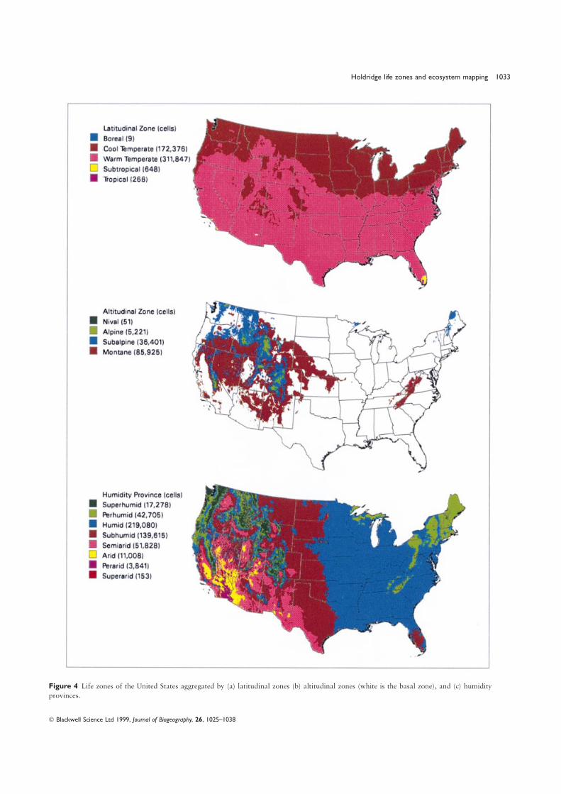
Results The US contains thirty-eight life zones (34% of the world’s life zones and 85% of

the temperate ones) including one boreal, twelve cool temperate, twenty warm temperate,

four subtropical, and one tropical. Seventy-four percent of the US falls in the ‘basal belt’,

18% is montane, 8% is subalpine, 1% is alpine, and < 0.1% is nival. The US ranges from

superarid to superhumid, and the humid province is the largest (45% of the US). The most

extensive life zone is the warm temperate moist forest, which covers 23% of the country.

We compared the Holdridge life zone map with output from the BIOME model, Bailey’s

ecoregions, Kuchler potential vegetation, and land cover, all aggregated to four cover

classes. Despite differences in the goals and methods for all these classification systems,

there was a very good to excellent agreement among them for forests but poor for grasslands,

shrublands, and nonvegetated lands.

Main conclusions We consider the life zone approach to have many strengths for ecosystem

mapping because it is based on climatic driving factors of ecosystem processes and recognizes

ecophysiological responses of plants; it is hierarchical and allows for the use of other

mapping criteria at the association and successional levels of analysis; it can be expanded

or contracted without losing functional continuity among levels of ecological complexity;

it is a relatively simple system based on few empirical data; and it uses objective mapping

criteria.

KeywordsEcosystem management, frost line, Holdridge, life zones, United States, vegetation mapping

1999 Blackwell Science Ltd

1026 A. E. Lugo et al.

INTRODUCTION vegetation and for assessing magnitudes of change as a result

of disturbances. However, the process of constructing theseA fundamental first step in designing ecosystem management

types of maps often involves circular reasoning. In the absenceis the delineation and classification of ecologically homogeneous

of comprehensive climatic information, vegetation is used deunits. To identify the basic attributes of the system being

facto as a surrogate of climate. However, climate in turn is amanaged it is possible that such attributes could be derived

driver of climax vegetation (Odum, 1945; Daubenmire, 1956;from existing maps or classification schemes. This is a difficult

Whittaker, 1956). This problem also permeates many of thetask at any level of biological (organisms to associations) or

bio-geographical approaches to ecosystem mapping (Bailey,ecological complexity (life zones to latitudinal belts), or at any

1996).spatial scale from a small watershed to the entire United States.

Another problem is that many traditional vegetationPast efforts to classify and map ecosystems of the United States

classification systems are not sufficiently objective so thatinclude vegetation maps based on ecological studies, such as

different people do not always produce the same classificationthose for the eastern region by Braun (1950), maps of biomes

designation for a particular geographical space. Part of thebased on bio-geographical criteria by J. Aldrich of the U.S.

problem is that many of these classification systems are notFish and Wildlife Service (Smith, 1974; pp. 536–537), maps of

driven by empirical data and consider the natural driving forcespotential vegetation based on local knowledge and temperature

upon ecosystems only weakly. Moreover, these classificationcriteria (e.g. Kuchler, 1964) and maps of ‘life zones’ based on

systems require users to have experience with the applicabilitytemperature criteria such as Merriam’s (1898) life and crop

and quality of the data base, and then fail to provide explicitzone map. For early comparisons of these approaches see Odum

rules for deciding how to use information to classify ecosystems(1945) and Daniel et al. (1979).

(Bailey & Hogg, 1983). The result is that two people using theBailey has undertaken the most comprehensive effort to

same information can produce different ecosystem classificationclassify and map ecosystems of the United States. He devised

maps. The maps themselves have gone through rapid evolutiona hierarchical classification of ecosystems using the methods

(Bailey, 1976, 1989, 1996; Bailey & Cushwa, 1981; Bailey et al.,of geographers (Bailey, 1980, 1983, 1984, 1985, 1987, 1988,

1994).1989, 1995, 1996). This particular approach has been adopted

The Holdridge system for classifying world life zones orby many U.S. Government agencies (Bailey, 1988, , 1995;

plant formations (from now on Holdridge Life Zone System;McNab & Avers, 1994) and will receive particular attention in

Holdridge, 1967) overcomes many of the aforementionedthis article. Another similar effort is that of Omernik (1995)

weaknesses of available ecosystem classification systems andwho mapped the ecological areas and ecological regions of the

can be a useful tool for identifying ecological units (life zones).United States.

The Holdridge Life Zone System is simple and objectiveThe availability of computerized techniques for handling

requiring at the minimum only data on mean annuallarge, spatially referenced data bases (e.g. geographical

precipitation, mean annual biotemperature (Tbio), and elevation.information systems [GIS]), has increased greatly our power

We have three objectives in this paper: (1) to define the qualitiesto predict and map patterns of potential natural vegetation.

of an ecosystem classification system for mapping in relationFor example, the BIOME model (Prentice et al., 1992) predicts

to ecosystem management and show how the Holdridge Lifepotential vegetation based on variables such as mean coldest-

Zone System fulfills most of these requirements; (2) to developmonth temperature, growing season temperature, a drought

and describe a life zone map for the conterminous Unitedindex incorporating seasonality of precipitation, and available

States; and (3) to compare the map of Holdridge life zoneswater capacity of the soil. With a combination of satellite

with other classification and mapping efforts such as those forimagery and computer analysis techniques, it is now possible

ecoregions, global biome models (BIOME), potentialto map actual vegetation for most parts of the world as has

vegetation, and land cover.been done for US forests (Powell et al., 1993) and land cover

(Loveland et al., 1991).

Each of these efforts has strengths and weaknesses, and theyQUALITIES OF AN ECOSYSTEMare all used for some aspect of ecosystem management (cf.CLASSIFICATION SYSTEMDaniel et al., 1979). For example, the satellite images of land

cover are excellent for assessing ecosystems at particularManaging ecosystems involves managing the structure and

moments in time, but they require continuous updating becausefunction of ecological units sensu Tansley (1935) and Evans

land cover and uses change constantly. Satellite images are also(1956). The complexity implied in this task can be made

useful for validating land-cover and land-use models and formore effective if the units of management are as ecologically

monitoring purposes. Traditional vegetation mapping, whichhomogeneous as possible. This in turn depends on the

focused on mature or climax vegetation (Whittaker, 1956) andeffectiveness of the classification system. Classification systems

maps of potential vegetation (Kuchler, 1964) are useful forthat result in ecologically homogeneous units should be more

comparing actual vegetation with potential or matureeffective than those that result in ecologically heterogeneous

units because management treatments tend to be uniform and

the response of a homogeneous system is more likely to beCorrespondence: A. E. Lugo, International Institute of Tropical For-

uniform than that of a heterogeneous system. The classificationestry, USDA Forest Service, PO BOX 25000, Rıo Piedras, P.R. 00928–5000. system must be the following.

Blackwell Science Ltd 1999, Journal of Biogeography, 26, 1025–1038

Holdridge life zones and ecosystem mapping 1027

Based on geo-referenced quantitative data. The more evaluated relative to that base condition. Changes cannot

be detected or established objectively if ecosystem states areempirically driven the system is, the less subjective it will be

and the more potential it has for improvement as more and compared to a subjective or continuously shifting initial

condition.better quality data become available.

As objective as possible. It is impossible for an ecosystem Applicable to all the world. Because there are no boundaries

to the function of ecosystems in the biosphere, an ecosystemclassification system to be completely objective because we lack

complete knowledge about the geographical distribution of classification system has to be applicable to the whole world.

This means that it has to account for changes in ecosystemvariables used for classifying ecological units. Subjectivity will

be reduced by the degree to which a classification system functioning across latitudinal belts.

is empirically driven and by stating classification rules and

assumptions explicitly. Demonstrably valid. An ecosystem classification system should

be validated with independent ecological data.

Reflect as closely as possible the forces driving ecosystems.

Ecosystems are basic units of ecology with arbitrary physical Conform to principles of climatic classification and vegetation

function. Climate is a major driver of vegetation distributionboundaries (Evans, 1956). Ecosystem function is driven

primarily by climatic factors, followed by edaphic, geomorphic, and ecosystem functioning (Schimper, 1903). An ecosystem

classification system must be based on climatic factors,and biotic factors. Therefore, ecosystem classification systems

that reflect the driving forces of ecosystems closely are more including climatic extremes and seasonality. An example is the

treatment of frost, which is critical for delimiting tropical andlikely to define the functional units of ecology than those that

attempt to define particular states or uses of ecosystems (i.e. subtropical ecosystems and determining the distribution and

richness of species (Schimper, 1903; Holdridge, 1967). Theforest or land-use types), or particular ecosystem size classes

(i.e., 105 km2 ecoregions). treatment of montane areas also requires special attention as

they are climatically heterogeneous (Daubenmire, 1952, 1956)

and contain complex environmental gradients (Brown &Hierarchical. Ecosystem function is hierarchical and includes

chemical, biological, ecological, and extraterrestrial hierarchies Curties, 1952; Hayward, 1952; Oosting & Reed, 1952;

Whittaker, 1956, 1960).of complexity. An ecosystem classification system has to be

hierarchical and contain units of classification that can be

aggregated or subdivided as seamlessly as possible so that by Accepts new data as a means to sharpen the analysis. Ecosystem

science is a rapidly evolving field which requires that ecosystemchanging the level of complexity few discontinuities in the

functioning and structuring of the system are introduced. classification systems be open for improvement. Ideally, a map

designation should change only as new empirical data becomeArbitrary hierarchies based on rules of size or area, i.e. powers

of 10, contain too much ecological heterogeneity and no matter available.

how convenient size hierarchies might be, their use introduces

discontinuities and reduce the effectiveness of ecosystemTHE HOLDRIDGE LIFE ZONE SYSTEM

management. A manager may treat an ecosystem type as if it

was a homogeneous unit when in fact it may be heterogeneous. The main advantage of the Holdridge Life Zone System (Fig. 1)

is that it is empirically and objectively based. Life zonesThe occurrence of homogeneous units of ecological function

is size-independent and can be one, or one thousand square are the main ecological unit of classification and they define

conditions for ecosystem functioning. Life zones are delimitedkilometers in area. In fact, Whittaker (1953) stated (p. 56):

‘Areal extent is irrelevant to achievement of the climax steady by biotemperature, precipitation, potential evapotranspiration

ratio, and elevation (see methods for definitions andstate, however; and there is no lower limit on the area of a

climax type.’ explanations). Any person using the system and having access

to the same data will classify a life zone the same way. There

is little room for subjectivity. The life zone system is hierarchicalConvenient for expanding or contracting complexity scales.

Because ecosystem management takes place at many scales of in that life zones can be subdivided into associations according

to site conditions including more detailed climatic data,ecological complexity, an ecosystem classification scheme

should be flexible and capable of expanding or contracting to atmospheric conditions, edaphic conditions, topography, and

aspect (Holdridge, 1967). Associations can be subdividedgreater or lesser scales of complexity. This is achieved by

aggregating or segregating its classification units while further into successional stages that reflect land use,

management, or disturbance history. Life zones can bemaintaining continuity with the functioning of the resulting

ecosystems. aggregated into larger humidity provinces, or belts of altitude

and/or latitude. The latitudinal belts reflect the utility of the

system for global scale ecosystem classification, while theUseful for anticipating global climate change. The environment

in which natural resources managers now operate requires altitudinal belts show it application to the complex montane

conditions.sensitivity to global climate change. To satisfy this requirement

the system has to be based on measures of climate so that a The Holdridge Life Zone System contains ecological and

ecophysiological constraints. For example, Holdridge reasonedreliable base condition can be established. Then change can be



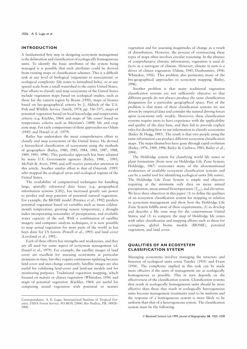
Figure 1 The life zone chart of Holdridge (1967). Consult text for further explanation.

that net primary productivity ceases at temperatures below & Lindsey (1964) in the United States; and the work we report

here.0 °C and above 30 °C. The ratio of potential evapotranspiration

to precipitation reflects water availability for ecological With regards to the second criticism, L.R. Holdridge

addressed this in a letter to A.A. Lindsey as follows:functions. The relationship between climatic parameters and

life zone delineation are logarithmic in recognition of limiting ‘The life zone system does not or should not pretend to

delineate homogeneous communities or associations offactor kinetics (Holdridge, 1967).

The Holdridge Life Zone System has been used to map the vegetation. The life zone is a climatic division defined by

biotemperature, precipitation, potential evapotranspiration,life zones of some 20 countries, including parts of the United

States (Sawyer, 1963; Sawyer & Lindsey, 1964; Brown & Lugo, and elevation in a logarithmic system which makes all life

zones equivalent in significance. Within each life zone there1980). A life zone map of the world has also been produced

and used to estimate the effects of global climate change on may be several vegetation associations dependent on soils,

lesser climatic variables and the presence or absence of openthe distribution of life zones (Emanuel et al., 1985); however,

the resolution of the map was coarse, altitudinal belts were water. The one climatic association of each life zone wherein

none of the secondary variations are significant, correspondsnot considered, and attention to frost or limiting temperature

line was poor. to a zonal soil and zonal climate. This, of course, may or may

not be present in an area where the life zone is present, butThe Holdridge Life Zone System has been criticized for

three reasons: (1) it is viewed as a system for classifying only since the physiognomy of the climatic association most clearly

typifies the life zone it has been utilized on the chart as a nametropical ecosystems (2) life zone names do not always coincide

with observed vegetation, i.e. grasslands appear in areas for the life zone.’

In other words, the Holdridge life zone map depicts theclassified as forests, and (3) it does not consider the seasonality

of climatic parameters. The first criticism is not valid as climatic conditions for ecosystem function and not the state of

the land at a particular time. The name of the life zone is notevidenced by the mapping of the world life zones for application

to global climate change issues (Emanuel et al., 1985; Solomon intended to mean that a particular vegetation is to be found

in a particular location. For example, the llanos of Venezuela& Shugart, 1993); the early work of Sawyer (1963), and Sawyer



are classified as tropical dry forest, but a considerable fraction METHODSof the vegetation is tropical savanna due to edaphic conditions

Climate data(Ewel & Madriz, 1968). Thus, while the climate could support

forest growing on a zonal soil, the local conditions modifyPrecipitationthe response of vegetation into savanna. These situations areThe spatial resolution chosen for this study (2.5 arc-minute forresolved at the association, rather than the life zone, level ofclassification, 4-km for mapping) was driven by the availabilitythe hierarchy.of accurate, reliable, documented, and archived precipitationThe third criticism of the Holdridge Life Zone System isdata. The current state-of-the-art in spatially distributedcorrect as climatic seasonality is not considered whenprecipitation modelling is provided by the Precipitation-identifying life zones at the first level of the hierarchy. Thiselevation Regressions on Independent Slopes Model or PRISMproblem becomes critical when comparing two regions with(Daly et al., 1994). The latest version of PRISM output for thesimilar average annual precipitation and biotemperature butcontiguous United States was downloaded from the Internetwhere one of them has a strong seasonality of rainfall or(ftp://fsl.orst.edu/pub/daly/prism/). This data set containswhere one has a wet winter and dry summer (e.g. in themonthly long-term average (1961–90) precipitation totals at a

western USA). This situation would have to be resolved at2.5 arc-minute grid resolution. The data set also provides the

the level of the association when other climatic variablesDigital Elevation Model (DEM) which was used to interpolate

are assessed.the precipitation data within the PRISM model.

The designation of Holdridge life zones automatically

includes consideration of their water balance and thus, the Temperatureinputs of rainfall and outputs of runoff and evapotranspiration Air temperature surfaces were obtained from the Vegetation/are incorporated into the classification. Wetlands, including Ecosystem Modelling and Analysis Project (VEMAP) (ftp://mangroves, respond to life zone conditions (Lugo & Cintron, ftp.ucar.edu:/cgd/vemap/). This accepted-standard data set1975; Weaver, 1987; Lugo et al., 1995). However, to assess the provides monthly long-term average minimum and maximumeffect of life zones in aquatic ecosystems fully, one has to air temperature surfaces for the contiguous United States at aconsider the relative influence of the different life zones within 30-arc-minute (approximately 50 km) grid resolution, derivedthe watershed boundaries of the aquatic system. from measurements at 4613 meteorological stations (Kittel

The Holdridge Life Zone System has been used for numerous et al., 1995). These temperature surfaces were enhanced to aecosystem management applications or to organize data, finer grid resolution by distributing the 30-arc-minuteincluding: evaluation of the effects of potential global climate temperature data over the topography of the 2.5-arc-minutechange on vegetation distribution (Emanuel et al., 1985; DEM from the PRISM data set. Using the Neutral StabilitySolomon & Shugart, 1993), carbon storage in tropical forests Algorithm, a method of spatial interpolation that explicitly(Brown & Lugo, 1982), analysis of global soil carbon and accounts for the relation between elevation and temperaturenitrogen content (Post et al., 1982, , 1985), land use and (Dodson & Marks, 1997), the centroids of the 30-arc-minutemanagement (Tosi, 1980), evaluation of human population temperature grid cells were interpolated to the resolution ofdistributions (Tosi & Voertman, 1964), and other issues such the PRISM DEM, resulting in a set of air temperature surfacesas predicting land productivity (Tosi, 1980) or evaluating which are compatible with the PRISM precipitation data (i.e.ecosystem complexity and species richness (Lugo & Brown, which correspond to the same 2.5 arc-minute DEM). Monthly

1991). mean air temperature surfaces were obtained by averaging the

minimum and maximum surfaces for each month.Life zone maps for the eastern and central United States

have been developed (Sawyer, 1963; Sawyer & Lindsey, 1964)Frost linebut they were based on a limited amount of information,The presence of frost defines the boundary between the warmparticularly climatic data for locations at high elevations. Intemperate and subtropical life zones in the HoldridgeSawyer’s early work, he found eleven life zones withinclassification. A frost line (delineation of frost-free and frost-four latitudinal regions (cool temperate, warm temperate,prone zones) was developed for the contiguous United Statessubtropical, and tropical) in the eastern and central Unitedfrom long-term daily measurements of minimum airStates. A particular problem with this early effort was thetemperature. Daily meteorological station data were obtainedomission of life zones at high elevations due to a lack offrom the National Climatic Data Center (ftp://data. Sawyer & Lindsey (1964) observed that scale difficultiesftp.ncdc.noaa.gov/pub/data/fsod/) where the data areprevented them from showing life zones that covered smallmaintained, documented, and archived. Stations that did notareas at higher elevations. Today, with larger and morehave at least 20 full years of daily minimum temperature data

extensive data bases, GIS technology, and fast computers, itduring the period 1960–95 were excluded, leaving 394 stations

is possible to make maps with greater accuracy and precisionthat were distributed reasonably evenly across the United States.

so that life zones with limited geographical extension canThe average number of frost days per year was computed for

be identified. Technological development is another argumenteach station location:

in favour of classifying ecosystems based on geo-referenced

data because it allows managers to be more precise in theirFmean=

sum(Fdays)

Nyears(1)

assessments.



where Fmean is the mean number of frost days per year, Fdays

is the number of days where Tmin was less than 0.0 C, and

Nyears is the length of the climate record in years. The 394

point measurements of Fmean were interpolated to a 4-km grid

by inverse-squared-distance (using eight nearest neighbours,

no maximum distance). A more elaborate elevation-sensitive

interpolation was not used here because (1) the sparseness of

the stations do not warrant it and (2) the boundary between

warm temperate and subtropical regions in the USA is restricted

to the lower elevations. The no-frost zone was then defined as

the set of grid cells where Fmean is less than 0.5, i.e. cells

which averaged less than one frost day per year (for at least

20 years in the period 1960–95). The 4-km frost line grid was

projected to a 2.5-minute latitude/longitude grid for

compatibility with the temperature and precipitation surfaces.

We followed this procedure without exception for our map.

We are generally confident that that this procedure projected

the frost line well, except for areas in south Florida where we

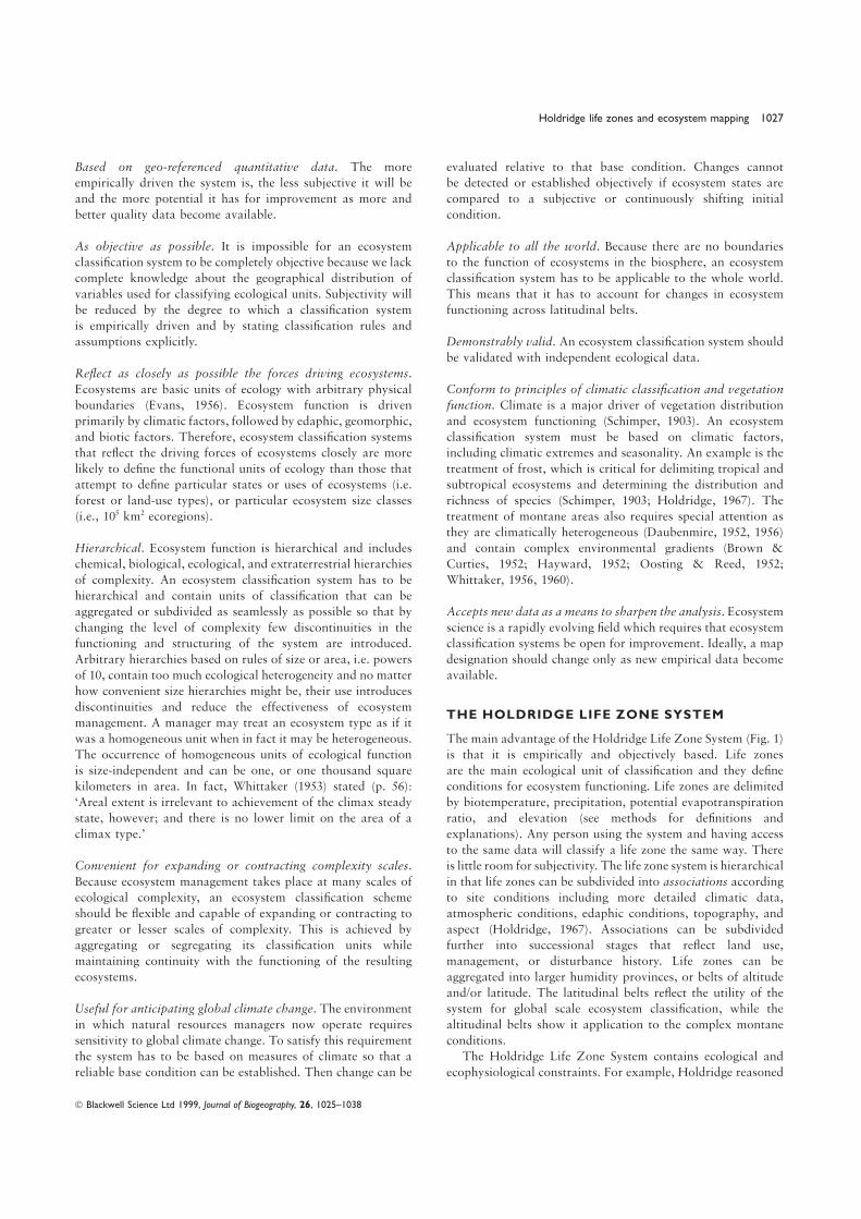
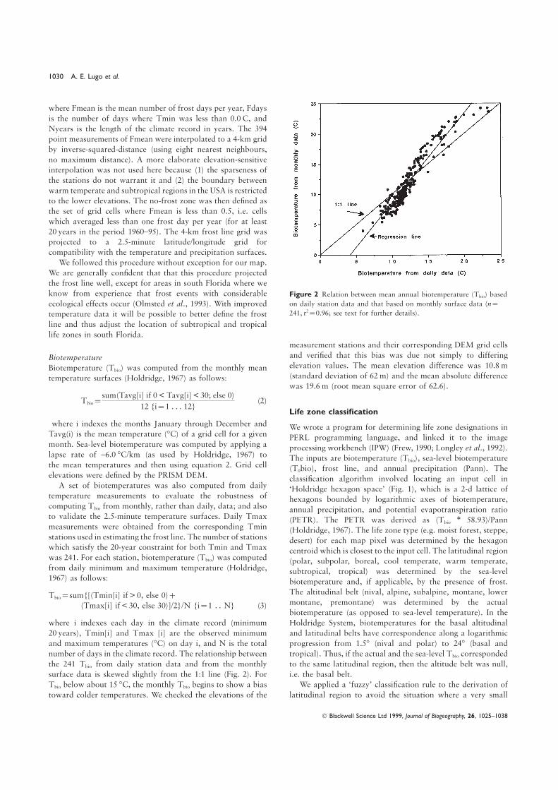
know from experience that frost events with considerable Figure 2 Relation between mean annual biotemperature (Tbio) based

on daily station data and that based on monthly surface data (n=ecological effects occur (Olmsted et al., 1993). With improved241, r2=0.96; see text for further details).temperature data it will be possible to better define the frost

line and thus adjust the location of subtropical and tropical

life zones in south Florida.

measurement stations and their corresponding DEM grid cells

and verified that this bias was due not simply to differingBiotemperatureelevation values. The mean elevation difference was 10.8 mBiotemperature (Tbio) was computed from the monthly mean(standard deviation of 62 m) and the mean absolute differencetemperature surfaces (Holdridge, 1967) as follows:was 19.6 m (root mean square error of 62.6).

Tbio=sum(Tavg[i] if 0 < Tavg[i] < 30; else 0)

12 {i=1 . . . 12}(2)

Life zone classificationwhere i indexes the months January through December and We wrote a program for determining life zone designations in

Tavg(i) is the mean temperature (°C) of a grid cell for a given PERL programming language, and linked it to the imagemonth. Sea-level biotemperature was computed by applying a processing workbench (IPW) (Frew, 1990; Longley et al., 1992).lapse rate of –6.0 °C/km (as used by Holdridge, 1967) to The inputs are biotemperature (Tbio), sea-level biotemperaturethe mean temperatures and then using equation 2. Grid cell (T0bio), frost line, and annual precipitation (Pann). Theelevations were defined by the PRISM DEM. classification algorithm involved locating an input cell in

A set of biotemperatures was also computed from daily ‘Holdridge hexagon space’ (Fig. 1), which is a 2-d lattice oftemperature measurements to evaluate the robustness of hexagons bounded by logarithmic axes of biotemperature,computing Tbio from monthly, rather than daily, data; and also annual precipitation, and potential evapotranspiration ratioto validate the 2.5-minute temperature surfaces. Daily Tmax (PETR). The PETR was derived as (Tbio ∗ 58.93)/Pannmeasurements were obtained from the corresponding Tmin (Holdridge, 1967). The life zone type (e.g. moist forest, steppe,stations used in estimating the frost line. The number of stations desert) for each map pixel was determined by the hexagonwhich satisfy the 20-year constraint for both Tmin and Tmax centroid which is closest to the input cell. The latitudinal regionwas 241. For each station, biotemperature (Tbio) was computed (polar, subpolar, boreal, cool temperate, warm temperate,from daily minimum and maximum temperature (Holdridge, subtropical, tropical) was determined by the sea-level1967) as follows: biotemperature and, if applicable, by the presence of frost.

The altitudinal belt (nival, alpine, subalpine, montane, lowerTbio=sum{[(Tmin[i] if > 0, else 0)+montane, premontane) was determined by the actual(Tmax[i] if < 30, else 30)]/2}/N {i=1 . . N} (3)biotemperature (as opposed to sea-level temperature). In the

Holdridge System, biotemperatures for the basal altitudinalwhere i indexes each day in the climate record (minimum

20 years), Tmin[i] and Tmax [i] are the observed minimum and latitudinal belts have correspondence along a logarithmic

progression from 1.5° (nival and polar) to 24° (basal andand maximum temperatures (°C) on day i, and N is the total

number of days in the climate record. The relationship between tropical). Thus, if the actual and the sea-level Tbio corresponded

to the same latitudinal region, then the altitude belt was null,the 241 Tbio from daily station data and from the monthly

surface data is skewed slightly from the 1:1 line (Fig. 2). For i.e. the basal belt.

We applied a ‘fuzzy’ classification rule to the derivation ofTbio below about 15 °C, the monthly Tbio begins to show a bias

toward colder temperatures. We checked the elevations of the latitudinal region to avoid the situation where a very small



Table 1 Biotemperature (Tbio) thresholds for latitudinal regions. See DISCUSSIONtext for the meaning of terms.

We examined four other types of ecosystem classificationLatitudinal regions Original Fuzzy systems and maps to verify and evaluate the Holdridge map.

These other classification systems included: the Loveland et al.Subpolar 1.5 1.68 (1991) land-cover map based on AVHRR (Advanced Very HighBoreal 3.0 3.36 Resolution Radiometer) satellite images, Baileys ecoregionsCool temperate 6.0 6.72

map, BIOME model output (Prentice et al., 1992), and KuchlersWarm temperate/Subtropical 12.0 13.44

(1964) potential vegetation map. Although all these mapsTropical 24.0 26.89

attempt to classify the land in some way, they do so from

different perspectives, thus one would not expect perfect

agreements among them. For example, Bailey’s map classifieschange in sea-level Tbio changes the overall life zonelarge scale ecological units much like the life zone map does,classification. For example, a site with Pann=500 mm, Tbio=BIOME’s map shows model output of potential vegetation5.95 °C, and T0bio=6.05 °C would be classified, under thebased on similar climatic variables as the life zone system,traditional method, as ‘cool temperate subalpine moist forest’,Loveland et al. s map shows present land cover/land use, andalthough the difference between actual and sea-level Tbio wasKuchler’s map shows potential vegetation.caused by an elevation of only 17 m (using the –6 °C/km lapse

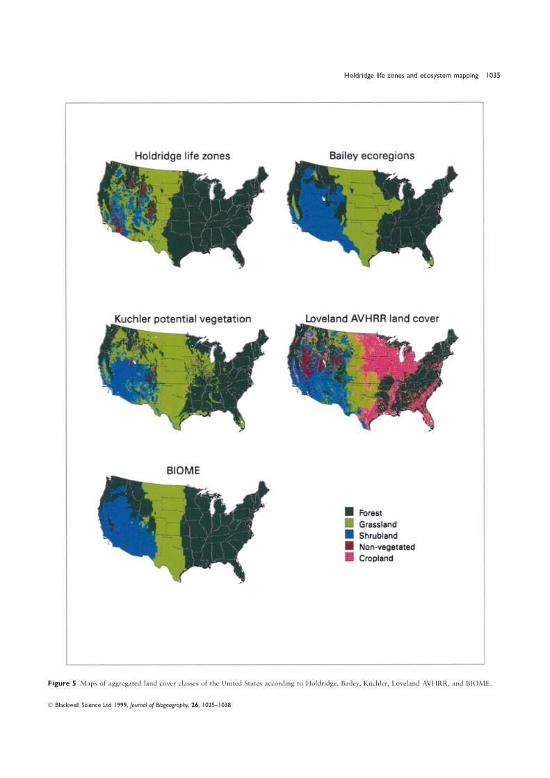
All maps were aggregated to four categories to allow for arate). Under our fuzzy rule, the sea-level Tbio is not permittedcommon base of comparison (forest, crop land, grassland, andto change the life zone unless it extends far enough into theshrubland; Fig. 5) and the Kappa-statistic (Monserud &next latitudinal region to be significant. ‘Significant’ thresholdLeemans, 1992) was computed for all classes overall as well asvalues were defined as the Tbio value of the lower-most hexagonfor individual classes (Table 3). There was fair to good agreementvertex of each row of hexagons in Holdridge space (Table 1).overall among the maps, except with Loveland et al. ′s. It is notThus, under the fuzzy rule, the example site would be classifiedsurprising that Loveland et al. ′s map had the poorest agreementas ‘boreal moist forest’.among all because it shows present day land cover/land use which

was not the goal of any of the other classification systems. TheRESULTS map that most closely agreed with the life zone map was BIOME

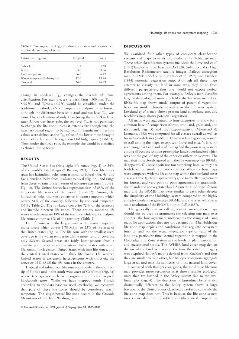
(Kappa=0.47), once again not too surprising because they areThe United States has thirty-eight life zones (Fig. 3) or 34%both based on similar climatic variables. When the four mapsof the world’s total (Lugo & Brown, 1991). These life zoneswere compared with the life zone map within the four land coverspan five latitudinal belts from tropical to boreal (Fig. 4a) andclasses (Table 3), they displayed very good to excellent agreementfive altitudinal belts from lowland to nival (Fig. 4b), and rangefor forests, and very poor to poor agreement for grasslands,from desert to rain forest in terms of moisture extremes (Table 2,shrublands and nonvegetated land. Again the Holdridge life zoneFig. 4c). The United States has representatives of 85% of themap and the BIOME map were similar to each other despitetemperate life zones of the world (Table 2). Among thethe simplicity of the Holdridge system compared to the highlylatitudinal belts, the most extensive is warm temperate whichcomplex model that generates BIOME, and the relatively coarsecovers 64% of the country, followed by the cool temperatescale resolution of the BIOME output (0.5°×0.5°).(35%; Table 2). The lowlands comprise 72% of the territory

The generally low overall agreement among these mapsand include nineteen life zones. There are six montane lifeshould not be used as arguments for selecting one map overzones which comprise 18% of the territory while eight subalpineanother; the low agreement underscores the danger of usinglife zones comprise 9% of the territory (Table 2).maps for applications they are not designed for. The HoldridgeThe life zone with the largest area is the warm temperatelife zone map depicts the conditions that regulate ecosystemmoist forest which covers 1.78 Mkm2 or 23% of the area offunction and not the actual vegetation type or state of thethe United States (Fig. 3). The life zone with the smallest arealland at a particular time. Actual vegetation is mapped in thecoverage is the warm temperate alpine moist tundra, coveringHoldridge Life Zone system at the levels of plant associationonly 32 km2. Several areas are fairly homogeneous from aand successional status. The AVHRR land-cover map depictsclimatic point of view: south-eastern United States with seventhe use of the land as it was at the time the satellite imagerylife zones, north-eastern United States with four life zones, andwas acquired. Bailey’s map is derived from Kuchler’s and thusthe central United States with three life zones. The westernthey are similar to each other, but Bailey’s ecoregions aggregateUnited States is extremely heterogeneous with thirty-six lifelarge areas and miss the subtleties of most natural land cover.zones or 95% of all the life zones in the country.

Compared with Bailey’s ecoregions, the Holdridge life zoneTropical and subtropical life zones occur only in the southernmap provides more resolution as it shows smaller ecologicaltip of Florida and in the south-west coast of California (Fig. 4a)units that are lumped in the Bailey system due to the size-where tree species such as mangroves and other tropicallimit rules (Fig. 6). The depiction of latitudinal belts is alsohardwoods grow. While we have mapped south Florida

dramatically different as the Bailey system shows a largeaccording to the data base we used (methods), we recognize

fraction of the United States classified as subtropical while thethat part of these life zones should be considered warm

life zone map does not. This is because the life zone systemtemperate. The single boreal life zone occurs in the Cascade

Mountains of northern Washington. uses a strict definition of subtropical (the critical temperature



Figure 3 Life zone map for the United States based on enhanced VEMAP climate data; 2.5 arc-minute resolution or approximately 4 km× 4 km

resolution.



Figure 4 Life zones of the United States aggregated by (a) latitudinal zones (b) altitudinal zones (white is the basal zone), and (c) humidity

provinces.



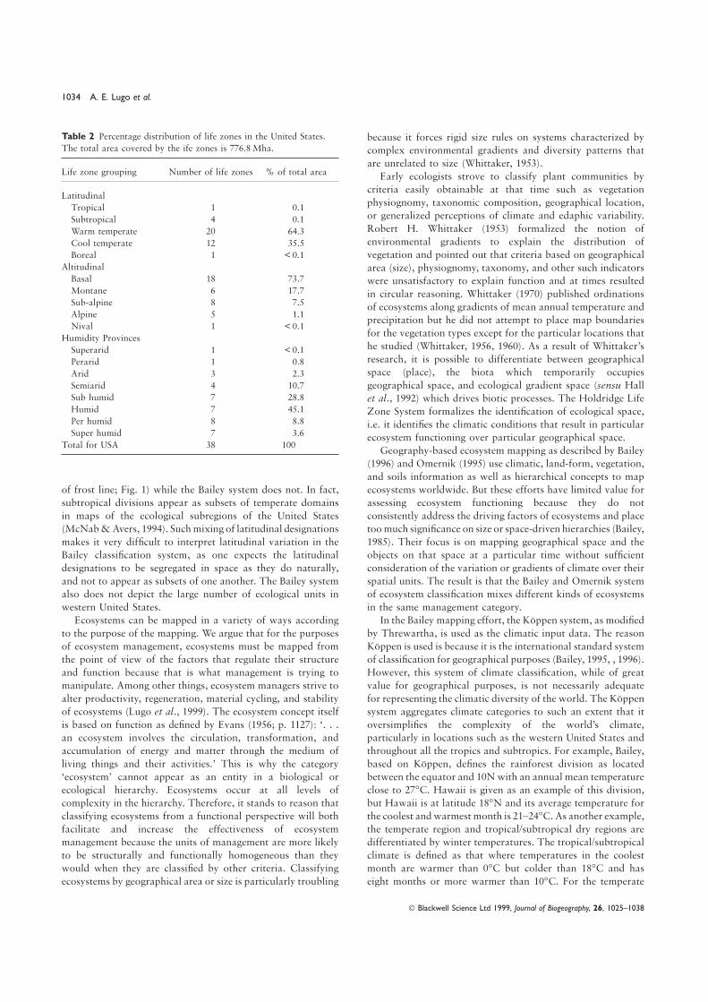
Table 2 Percentage distribution of life zones in the United States. because it forces rigid size rules on systems characterized byThe total area covered by the ife zones is 776.8 Mha. complex environmental gradients and diversity patterns that

are unrelated to size (Whittaker, 1953).Life zone grouping Number of life zones % of total area Early ecologists strove to classify plant communities by

criteria easily obtainable at that time such as vegetationLatitudinal

physiognomy, taxonomic composition, geographical location,Tropical 1 0.1

or generalized perceptions of climate and edaphic variability.Subtropical 4 0.1Robert H. Whittaker (1953) formalized the notion ofWarm temperate 20 64.3environmental gradients to explain the distribution ofCool temperate 12 35.5

Boreal 1 < 0.1 vegetation and pointed out that criteria based on geographicalAltitudinal area (size), physiognomy, taxonomy, and other such indicators

Basal 18 73.7 were unsatisfactory to explain function and at times resultedMontane 6 17.7 in circular reasoning. Whittaker (1970) published ordinationsSub-alpine 8 7.5 of ecosystems along gradients of mean annual temperature andAlpine 5 1.1

precipitation but he did not attempt to place map boundariesNival 1 < 0.1

for the vegetation types except for the particular locations thatHumidity Provinces

he studied (Whittaker, 1956, 1960). As a result of Whittaker’sSuperarid 1 < 0.1research, it is possible to differentiate between geographicalPerarid 1 0.8space (place), the biota which temporarily occupiesArid 3 2.3

Semiarid 4 10.7 geographical space, and ecological gradient space (sensu HallSub humid 7 28.8 et al., 1992) which drives biotic processes. The Holdridge LifeHumid 7 45.1 Zone System formalizes the identification of ecological space,Per humid 8 8.8 i.e. it identifies the climatic conditions that result in particularSuper humid 7 3.6 ecosystem functioning over particular geographical space.

Total for USA 38 100Geography-based ecosystem mapping as described by Bailey

(1996) and Omernik (1995) use climatic, land-form, vegetation,

and soils information as well as hierarchical concepts to map

ecosystems worldwide. But these efforts have limited value forof frost line; Fig. 1) while the Bailey system does not. In fact,

subtropical divisions appear as subsets of temperate domains assessing ecosystem functioning because they do not

consistently address the driving factors of ecosystems and placein maps of the ecological subregions of the United States

(McNab & Avers, 1994). Such mixing of latitudinal designations too much significance on size or space-driven hierarchies (Bailey,

1985). Their focus is on mapping geographical space and themakes it very difficult to interpret latitudinal variation in the

Bailey classification system, as one expects the latitudinal objects on that space at a particular time without sufficient

consideration of the variation or gradients of climate over theirdesignations to be segregated in space as they do naturally,

and not to appear as subsets of one another. The Bailey system spatial units. The result is that the Bailey and Omernik system

of ecosystem classification mixes different kinds of ecosystemsalso does not depict the large number of ecological units in

western United States. in the same management category.

In the Bailey mapping effort, the Koppen system, as modifiedEcosystems can be mapped in a variety of ways according

to the purpose of the mapping. We argue that for the purposes by Threwartha, is used as the climatic input data. The reason

Koppen is used is because it is the international standard systemof ecosystem management, ecosystems must be mapped from

the point of view of the factors that regulate their structure of classification for geographical purposes (Bailey, 1995, , 1996).

However, this system of climate classification, while of greatand function because that is what management is trying to

manipulate. Among other things, ecosystem managers strive to value for geographical purposes, is not necessarily adequate

for representing the climatic diversity of the world. The Koppenalter productivity, regeneration, material cycling, and stability

of ecosystems (Lugo et al., 1999). The ecosystem concept itself system aggregates climate categories to such an extent that it

oversimplifies the complexity of the world’s climate,is based on function as defined by Evans (1956; p. 1127): ‘. . .

an ecosystem involves the circulation, transformation, and particularly in locations such as the western United States and

throughout all the tropics and subtropics. For example, Bailey,accumulation of energy and matter through the medium of

living things and their activities.’ This is why the category based on Koppen, defines the rainforest division as located

between the equator and 10N with an annual mean temperature‘ecosystem’ cannot appear as an entity in a biological or

ecological hierarchy. Ecosystems occur at all levels of close to 27°C. Hawaii is given as an example of this division,

but Hawaii is at latitude 18°N and its average temperature forcomplexity in the hierarchy. Therefore, it stands to reason that

classifying ecosystems from a functional perspective will both the coolest and warmest month is 21–24°C. As another example,

the temperate region and tropical/subtropical dry regions arefacilitate and increase the effectiveness of ecosystem

management because the units of management are more likely differentiated by winter temperatures. The tropical/subtropical

climate is defined as that where temperatures in the coolestto be structurally and functionally homogeneous than they

would when they are classified by other criteria. Classifying month are warmer than 0°C but colder than 18°C and has

eight months or more warmer than 10°C. For the temperateecosystems by geographical area or size is particularly troubling



Figure 5 Maps of aggregated land cover classes of the United States according to Holdridge, Bailey, Kuchler, Loveland AVHRR, and BIOME.



Table 3 Degree of agreement among the different classification ecosystem functioning on that site. Size or area prejudgementsmaps and the Holdridge Life Zone map based on the Kappa-statistic are removed and the ecosystem manager can deal directly(Monserud & Leemans, 1992)∗. with the biota of interest. On this climatic foundation other

modifying factors can be overlain as required of any hierarchicala. Overall Kappa Holdridge Bailey Kuchler Loveland

system of ecosystem classification and management.

Holdridge 1.0

Bailey 0.39 1.0 ACKNOWLEDGMENTSKuchler 0.43 0.69 1.0

Loveland 0.25 0.41 0.37 1.0 The information in this document has been funded by the U.S.BIOME 0.47 0.71 0.60 0.37 Environmental Protection Agency, by a contract (number 68-

C6–0005) between US EPA and Dynamac Corporation, and inb. Kappa by vegetation Holdridge cooperation with the University of Puerto Rico as part of thegroup

USDA Forest Service contribution to the Long-term EcologicalForest Grassland Shrubland Non-

Research Program of the National Science Foundation. Wevegetated

thank J. Francis, F. Scatena, and C. A. Hall for helpful

comments on the manuscript, D. P. Turner for contributionsBailey 0.83 0.21 0.24 –to the development of the 4-km climate data set, Olga RamosKuchler 0.87 0.26 0.29 0.39for helping with the GIS, and M. Alayon. The manuscript hasLoveland 0.87 0.41 0.16 0.07

BIOME 0.76 0.42 0.22 0.44 been subjected to the EPA’s peer and administrative review,

and it has been approved for publication as an EPA document.∗Kappa statistic: 0.00–0.05=no agreement; 0.05–0.20=very poor; Mention of trade names or commercial products does not0.20–0.40=poor; 0.40–0.55=fair; 0.55–0.70=good; 0.70–0.85=very

constitute endorsement or recommendation for use.good; 0.85–0.99=excellent; 0.99–1.00=perfect agreement

REFERENCES

Bailey, R.G. (1976) Ecoregions of the United States. Map. USDA Forest

Service Intermountain Station, Ogden, UT.

Bailey, R.G. (1980) Description of the ecoregions of the United States.

USDA Forest Service Miscellaneous Publication no. 1391.

Bailey, R.G. (1983) Delineation of ecosystem regions. Environ. Mgmnt,

7, 365–373.

Bailey, R.G. (1984) Testing and ecosystem regionalization. J. Environ.

Mgmnt, 19, 239–248.

Bailey, R.G. (1985) The factor of scale in ecosystem mapping. Environ.

Mgmnt, 9, 271–276.

Bailey, R.G. (1987) Suggested hierarchy of criteria for multi-scale

ecosystem mapping. Landscape Urban Planning, 14, 313–319.

Bailey, R.G. (1988) Ecographic analysis a guide to the ecological

division of land for resource management. USDA Forest Service

Miscellaneous Publication 1465, Washington, D.C.

Bailey, R.G. (1989) Explanatory (Suppl.)to Ecoregions Map of the

Continents. Environ. Conserv. 16, 307–309.Figure 6 Rank order by area of the thirty-eight life zones of the

Bailey, R.G. (1995) Description of the ecoregions of the United States.United States and the ecological provinces of Bailey et al. (1994).

USDA Forest Service Miscellaneous Publication 1391. Washington,

D.C.

Bailey, R.G. (1996) Ecosystem geography. Springer Verlag, Heidelberg.,climate, on the other hand, the coldest month is cooler than New York.0°C and has 4–8 months warmer than 10°C. This definition of Bailey, R.G. & Cushwa, C.T. (1981) Ecoregions of North America.subtropical/temperate climates ignores the presence of regular Map. US Fish and Wildlife Service OBS-81/29, Washington, D.C.

Bailey, R.G. & Hogg, H.C. (1983) A world ecoregions map for resourcefrost which is the critical factor that delimits the distributionreporting. Environ. Conserv. 13, 195–202.of tropical/subtropical species from temperate ones. The result

Bailey, R.G., Avers, P.E., King, T. & McNab, W.H. (1994) Ecoregionsis that Bailey’s ecoregion maps show the United States as aand subregions of the United States. Map. USDA Forest Service,country with a very high representation of tropical/subtropicalWashington, D.C.regions, but without the biodiversity associated with these

Braun, E.L. (1950) Deciduous forests of eastern North America. Theclimates.

Blakiston Company, Philadelphia.In presenting the life zones of the United States, we have

Brown, R.T. & Curties, J.T. (1952) The upland conifer-hardwoodshown how to take advantage of empirical data bases to define forests of northern Wisconsin. Ecol. Monogr. 22, 217–234.the life zone condition over a geographical space upon which Brown, S. & Lugo, S.S. (1980) Preliminary estimate of the storage ofecosystems function. This removes subjectivity in mapping organic carbon on tropical forest ecosystems. The role of tropical

forests in the world carbon cycle (ed. by S. Brown, A. E. Lugo andwhile at the same time defining the potential and limits for



B. Liegel), pp. 65–117. CONF-800350 UC-11. US Department of Forest. Tropical forests: management and ecology (ed. by A. E. Lugo

and C. Lowe), pp. 142–177. Springer Verlag, New York.Energy, Office of Health and Environment Research, Washington,

DC. Lugo, A.E., Baron, J.S., Frost, T.P., Cundy, T.W. & Dittberner, P.

(1999) Ecosystem processes and functioning. Ecological Stewardship:Brown, S. & Lugo, A.E. (1982) The storage and production of organic

matter in tropical forests and their role in the global carbon cycle. A Common reference for Ecosystem Management, Vol. 2, Elsevier

Science, New York (ed. by N. C. Johnson, A. J. Malk, W. T. SextonBiotropica, 14, 161–187.

Daly, C., Neilson, R. P. & Phillips, D. L. (1994) A statistical-topographic and R. C. Szaro, editors).

McNab, W.H. & Avers, P.E. (1994) Ecological subregions of the Unitedmodel for mapping climatological precipitation over mountainous

terrain. J. appl. Meteor. 33, 140–158. States: section descriptions. USDA Forest Service, Administrative

Publication WO-WSA-5, Washington, D.C.Daniel, T.W., Helms, J.A. & Baker, F.S. (1979) Principles of silviculture.

McGraw-Hill, New York. Merriam, C. H. (1898). Life zones and crop zones of the United States.

US Department of Agriculture, Division of Biological Survey BulletinDaubenmire, R. (1952) Forest vegetation of northern Idaho. Ecol.

Monogr. 22, 301–330. 10, Washington, D.C.

Monserud, R.A. & Leemans, R. (1992) Comparing global vegetationDaubenmire, R. (1956) Climate as a determinant of vegetation dis-

tribution in eastern Washington and northern Idaho. Ecol. Monogr. maps with the Kappa-statistic. Ecol. Model. 62, 275–293.

Odum, E.P. (1945) The concept of the biome as applied to the dis-26, 131–154.

Dodson, R. & Marks, D. (1997) Daily air temperature interpolated at tribution of North American birds. Wilson Bull. 57, 191–201.

Olmsted, I., Dunevitz, H. & Platt, W. J. (1993) Effects of freezes onhigh spatial resolution over a large mountainous region. Climate

Res. 8, 1–20. tropical trees in Everglades National Park Florida, USA. Trop. Ecol.

34, 17–34.Emanuel, W.R., Shugart, H.H. & Stevenson, M.P. (1985) Climate

change and the broad-scale distribution of terrestrial ecosystem Omernik, J.M. (1995) Ecoregions: a spatial framework for en-

vironmental management. Biological assessment and criteria: toolscomplexes. Clim. Change 7, 29–43.

Evans, F.C. (1956) Ecosystems as the basic unit in ecology. Science, for water resource planning and decision making (ed. by W. S. Davis

and T. P. Simon), pp. 49–62. Lewis Publishers, Boca Raton.123, 1127–1128.

Ewel, J.J. & Madriz, A. (1968) Zonas de Vida de Venezuela + map. Oosting, H.J. & Reed, J.F. (1952) Virgin spruce-fir of the Medicine

Bowe Mountains, Wyoming. Ecol. Monogr. 22, 69–91.Editorial Sucre, Caracas.

Frew, J.E. (1990) The image processing workbench. PhD Dissertation. Post, W.M., Emanuel, W.R., Zinke, P.J. & Stangenberger, A. (1982)

Soil carbon pools and world life zones. Nature, 298, 156–159.University of California, Santa Barbara, CA.

Hall, C. A. S., Stanford, J. A. & Hauer, F. R. (1992) The distribution Post, W.M., Pastor, J., Zinke, P.J. & Stangenberger, A. (1985) Global

patterns of soil nitrogen storage. Nature, 317, 613–616.and abundance of organisms as a consequence of energy balances

along multiple environmental gradients. Oikos, 65, 377–390. Powell, D.S., Faulkner, J.L., Darr, D.R., Zhu, Z. & MacCleery, D.W.

(1993) Forest resources of the United States, 1992. USDA ForestHayward, C.L. (1952) Alpine biotic communities of the Uinta Moun-

tains, Utah. Ecol. Monogr. 22, 93–120. Service GTR RM-234, Rocky Mountain Forest and Range Ex-

periment Station, Fort Collins, CO.Holdridge, L.R. (1967) Life zone ecology. Tropical Science Center. San

Jose, Costa Rica. Prentice, C.I., Cramer, W., Harrison, S.P., Leemans, R., Monserud,

R.A. & Solomon, A.M. (1992) A global biome model based on plantKittel, T.G.F., Rosenbloom, N.A., Painer, T.H., Schimel, D.S. &

VEMAP, Modeling Participants. ((1995) The VEMAP integrated physiology and dominance, soil properties and climate. J. Biogeogr.

19, 117–134.database for modeling United States ecosystem/vegetation sensitivity

of climate change. J. Biogeogr. 22, 857–862. Sawyer, J.O. & Lindsey, A.A. (1964) The Holdridge bioclimatic form-

ations of the eastern and central United States. Proc. Indiana Acad.Koppen, W. (1931) Grundriss der klimakunde. Walter de Grwyter,

Berlin. Sci. 72, 105–112.

Sawyer, J.O. Jr (1963) The Holdridge system of bioclimatic formationsKuchler, A.W. (1964) Potential natural vegetation of the conterminous

United States + map. American Geographic Society Special Pub- applied to the eastern and central United States. Thesis, Purdue

University, Lafayette, Indiana.lication 36, New York.

Longley, K.D., Jacobsen, D. & Marks, D. (1992) (Suppl.)to the Image Schimper, A.F.W. (1903) Plant-geography upon a physiological basis.

English translation by W.R. Fisher. Clarendon Press, Oxford.Processing Workbench (IPW): modifications, procedures, and soft-

ware additions, Revision 2.0. Technical Report, EPA-COR EPA/600/ Smith, R.L. (1974) Ecology and field biology. Harper & Row, New

York, NY.9–92/217. U.S. Environmental Protection Agency, Environmental

Research Laboratory, Corvallis, OR. Solomon, A.M. & Shugart, H.H. (1993) Vegetation dynamics and

global change. Chapman & Hall, New York, NY.Loveland, T.R., Merchant, J.W., Ohlen, D.O. & Brown, J.F. (1991)

Development of a land-cover characteristics database for the con- Tansley, A.G. (1935) The use and abuse of vegetational concepts and

terms. Ecology, 16, 284–307.terminous US. Photogram. Engng Rem. Sens. 57, 1453–1463.

Lugo, A.E. & Cintron, G. (1975) The mangrove forests of Puerto Rico Tosi, J. (1980) Life zones, land use, and forest vegetation in the tropical

and subtropical regions. The role of tropical forests in the Worldand their management. Proceedings of International Symposium on

Biology and Management of Mangroves (ed. by G. Walsh, S. Snedaker carbon cycle (ed. by S. Brown, A. E. Lugo and B. Liegel), pp. 44–64.

CONF-800350 UC-11. US Department of Energy, Office of Healthand H. Teas), pp. 825–846. Institute of Food and Agricultural

Sciences, Gainesville, Fl. and Environment Research, Washington, DC.

Tosi, J. & Voertman, R.F. (1964) Some environmental factors in theLugo, A.E. & Brown, S. (1991) Comparing tropical and temperate

forests. Comparative analysis of ecosystems: patterns, mechanisms, economic development of the tropics. Econ. Geogr. 40, 189–205.

VEMAP Members (J.M. Melillo, J. Borchers, J. Chaney, H. Fisher, S.and theories (ed. by J. Cole, G. Lovett and S. Findlay), pp. 319–330.

Springer-Verlag, New York. Fox, A. Haxeltine, A. Janetos, D.W. Kicklighter, T.G.F. Kittel, A.D.

McGuire, R. McKeown, R. Neilson, R. Nemani, D.S. Ojima, T.Lugo, A.E., Bokkestijn, A. & Scatena, F.N. (1995) Structure, succession,

and soil chemistry of palm forests in the Luquillo Experimental Painter, Y. Pan, W.J. Parton, L. Pierce, L. Pitelka, C. Prentice, B.



Rizzo, N.A. Rosenbloom, S. Running, D.S. Schimel, S. Sitch, T. BIOSKETCHESSmith, I. Woodward) (1995) Vegetation/Ecosystem Modeling and

Analysis Project (VEMAP): Comparing biogeography and bi-

ogeochemistry models in a continental-scale study of terrestrial Ariel E. Lugo, PhD, is an ecologist and Director of theecosystem responses to climate change and CO2 doubling. Global USDA Forest Service International Institute of TropicalBiogeochem. Cycles, 9, 407–437. Forestry. His research activities have centred on the

Weaver, P.L. (1987) Structure and dynamics in the colorado forest of structure and function of mangrove forests and the role ofthe Luquillo Mountains of Puerto Rico. Dissertation. Michigan State tropical forests in the global carbon cycle. His currentUniversity, East Lansing, Michigan. interest is in the long term dynamics and management of

Whittaker, R.H. (1953) A consideration of climax theory: the climax tropical forests.as a population and pattern. Ecol. Monogr. 22, 41–78.

Whittaker, R.H. (1956) Vegetation of the Great Smokey Mountains.Sandra L. Brown is Professor of Forest Ecology at the

Ecol. Monogr. 26, 1–80.University of Illinois in Champaign-Urbana. Her research

Whittaker, R.H. (1960) Vegetation of the Siskiyou Mountains, Oregonexperience and interests centre on assessing the role of

and California. Ecol. Monogr. 30, 279–338.forests, particularly tropical ones, in the global carbonWhittaker, R.H. (1970). Communities and ecosystems. MacMillan,cycle, including estimating storages and flux of carbon inNew York.forests and how these change with changing land use and

human activities. She is also actively involved in several

roles with the IPCC.


Documents

The Holdridge life zones of the conterminous United States ... · The Holdridge life zones of the conterminous United States in relation to ecosystem ... the satellite images of land