Contents lists available at SciVerse ScienceDirect

Journal of Quantitative Spectroscopy &Radiative Transfer

Journal of Quantitative Spectroscopy & Radiative Transfer 113 (2012) 1372–1390

0022-40

doi:10.1

n Corr

fax: þ4

E-m

journal homepage: www.elsevier.com/locate/jqsrt

The Joint Airborne IASI Validation Experiment: An evaluation ofinstrument and algorithms

Stuart M. Newman a,n, Allen M. Larar b, William L. Smith c,d, Igor V. Ptashnik e,Roderic L. Jones f, Mohammed I. Mead f, Henry Revercomb d, David C. Tobin d,Joe K. Taylor d, Jonathan P. Taylor a

a Met Office, FitzRoy Road, Exeter EX1 3PB, United Kingdomb NASA Langley Research Center, Hampton, VA, USAc Hampton University, Hampton, VA, USAd University of Wisconsin-Madison, Madison, WI, USAe V.E. Zuev Institute of Atmospheric Optics, 1 Academician Zuev Square, Tomsk 634055, Russiaf Centre for Atmospheric Science, Department of Chemistry, University of Cambridge, Lensfield Road, Cambridge CB2 1EW, UK

a r t i c l e i n f o

Available online 3 March 2012

Keywords:

Remote sensing

Radiative transfer

Spectroscopy

Water vapor continuum

Interferometry

73/$ - see front matter & 2012 Elsevier Ltd. A

016/j.jqsrt.2012.02.030

esponding author. Tel.: þ44 1392 884605;

4 1392 885681.

ail address: stu.newman@metoffice.gov.uk (S

a b s t r a c t

The Joint Airborne IASI Validation Experiment (JAIVEx) was designed to investigate the

absolute radiometric accuracy of the Infrared Atmospheric Sounding Interferometer

(IASI) and test the radiative transfer algorithms on which applications using IASI

radiances rely. Two comprehensively instrumented research aircraft participated in

coordinated measurements co-aligned with overpasses on the IASI instrument, with

airborne interferometers obtaining radiance observations alongside intensive measure-

ments of the atmospheric state. The JAIVEx data set has been used to place an upper

bound on the absolute radiometric accuracy of IASI radiances. Further, a set of clear air

case studies have been used to test competing formulations of the CO2 line shape, water

vapor spectroscopic line parameters and continuum. The current state-of-the art

performance of line-by-line models is established with implications for optimal use

of IASI radiances in numerical weather prediction.

& 2012 Elsevier Ltd. All rights reserved.

1. Introduction

The Infrared Atmospheric Sounding Interferometer (IASI)was launched in October 2006 on the European satelliteMetOp-A. Together with the Atmospheric Infrared Sounder(AIRS) on NASA’s Aqua satellite it represents a new genera-tion of hyperspectral instruments used in NumericalWeather Prediction (NWP) [1]. (By hyperspectral we meanwith a spectral resolution of the order of 1 cm�1 which ismuch finer than has been possible before in meteorological

ll rights reserved.

.M. Newman).

sounding.) The goal of the IASI mission is to provide atmo-spheric emission/absorption spectra for the estimation oftropospheric temperatures to within 71 K and humidity towithin 710% at 1 km vertical resolution [2]. Trials at NWPcenters have shown a positive impact of assimilating IASIradiances at least as large as for any previously introducednew instrument (e.g. [3]). IASI is also designed for thecapability to retrieve trace gas total column amounts suchas CO2, O3, N2O, CO and CH4.

Nearly all applications of IASI require synthetic radiancesto be simulated using radiative transfer models, whichthemselves depend on knowledge of the underlying spec-troscopy of the atmospheric species that absorb and emitradiation in the infrared spectral region. It is important,therefore, to assess critically the capabilities of the current

S.M. Newman et al. / Journal of Quantitative Spectroscopy & Radiative Transfer 113 (2012) 1372–1390 1373

generation of radiative transfer codes and understand theirlimitations. One powerful technique is a radiative closureexperiment in which a combination of quality radianceobservations, well constrained measurements of the atmo-spheric state and line-by-line radiative transfer simulationsare brought to bear on the problem of identifying uncer-tainties in atmospheric radiance modeling.

In this work we analyze the clear sky data set collectedduring the Joint Airborne IASI Validation Experiment (JAI-VEx) in 2007, combining airborne and satellite interferom-eter measurements temporally and spatially co-located withintensive sampling of the atmospheric state. JAIVEx datahave already proved invaluable in testing the ability toretrieve fine-scale features with high vertical resolutionfrom IASI radiances [4], in retrievals of land surface emissiv-ities from airborne hyperspectral measurements [5], for thevalidation of the absolute radiometric performance of IASI[6] and in the development of novel applications suchas correlation interferometry for retrievals of CO2 columnamounts [7]. A key aim of JAIVEx was to validate theabsolute radiometric accuracy of IASI and we presentcomparisons of co-located interferometer radiances to con-strain the calibration uncertainty. Further, we seek to useobserved minus calculated spectral residuals to probeuncertainties due to spectroscopic line parameters and theformulation of the water vapor continuum.

This paper joins others in this special issue honoring thecontributions of three pre-eminent high-resolution molecu-lar spectroscopists: Jean-Marie Flaud, Claude Camy-Peyret,and Alain Barbe. It is notable that a great many aspects ofspectroscopy relevant to infrared hyperspectral soundinghave their foundations in the work of these pioneeringscientists. The optimum use of satellite hyperspectral mea-surements depends on an accurate knowledge of funda-mental spectroscopic parameters for gases such as H2O [8]and CO2 [9]. Their work has also been instrumental in thecalibration/validation of IASI [10] and subsequent studies onthe retrieval of atmospheric constituents from IASI spectra[11]. Perhaps most importantly, their numerous contribu-tions to extensively-used databases such as HITRAN [12]and GEISA [13] underpin the hyperspectral radiative trans-fer modeling which is the subject of this work.

In Section 2 we describe the JAIVEx campaign and themeasurement capabilities that were deployed, while themethodology for data analysis is outlined in Section 3. Theresults are subdivided into the following parts: in Section 4we quantify the IASI radiometric accuracy using two clearsky case studies; in Section 5 we present results comparingmodels of CO2 temperature sounding channels; and inSection 6 an atmospheric profile retrieval method is pre-sented for assessment of water vapor spectroscopy andcontinuum models, using IASI and aircraft interferometerdata sets. We conclude in Section 7.

2. JAIVEx campaign

The Joint Airborne IASI Validation Experiment (JAIVEx)was a collaborative campaign, bringing together researchgroups from the United States and the United Kingdom[6]. The campaign was based in Houston, Texas during

April–May 2007, shortly after the launch of IASI on MetOpin October 2006. Two research aircraft participated: theFAAM BAe 146-301 tropospheric research aircraft and theNASA WB-57 high altitude platform. Both are comprehen-sively instrumented facilities, well suited to satellite cali-bration/validation (cal/val) exercises of this kind. Flights ofthe two aircraft were coordinated with overpasses of IASIand AIRS [14], with sorties conducted over ocean (Gulf ofMexico) and over land (ARM Southern Great Plains facility,Oklahoma). This data set has been exploited to test theabsolute radiative accuracy of IASI and radiative transfermodels that underpin the use of satellite data in NWP.

The instrument capabilities for the campaign included

1.

Satellite radiance observations from MetOp-A: Clearsky measurements from IASI and the MicrowaveHumidity Sounder (MHS) were targeted for each casestudy. IASI is a passive infrared sounder operating inthe range of 645–2760 cm�1. Its optical configurationis based on a classical Michelson interferometer [15].The apodized ‘‘Level 1c’’ spectra have a sample spacingof 0.25 cm�1 (corresponding to 0.5 cm�1 resolution).

2.

Airborne interferometer observations: The WB-57aircraft carries two state-of-the-art interferometers:the Scanning High-resolution Interferometer Sounder(S-HIS) [16] measuring upwelling and downwellinginfrared radiances at high spectral resolution (spectralsampling 1/[2OPD]¼0.5 cm�1 where OPD is the opticalpath difference) and the National Polar-orbiting Opera-tional Environmental Satellite System (NPOESS) AirborneSounder Testbed-Interferometer (NAST-I) measuringupwelling radiances at 1/[2OPD]¼0.25 cm�1 [17]. Bothof these interferometers scan cross-track, i.e. measure aswath below the aircraft in a similar way to IASI onMetOp. The payload of the FAAM BAe 146 includes theAirborne Research Interferometer Evaluation System(ARIES) [18] which has similar spectral characteristicsto S-HIS. ARIES was directed to measure directly upwardand downward views during JAIVEx. Importantly, theseinterferometers have been calibrated against traceableabsolute standards at national metrology institutes intheir respective countries of origin. The instrumentcapabilities are summarized in Table 1.

3.

Dropsondes: The FAAM aircraft released numerousparachute-borne sondes (typically 12–15 per flight)for intensive atmospheric profiling. The Airborne Ver-tical Atmospheric Profiling System (AVAPS) allowedthe measurement of temperature, humidity, winds andGPS position which were transmitted back to a recei-ver on the aircraft.

4.

In situ sampling of chemistry species: The FAAM BAe146 measured in situ concentrations of O3 and COduring the JAIVEx flying. A prototype tunable diodelaser absorption spectrometer (TDLAS) instrumentfrom the University of Cambridge was also deployedenabling the measurement of CO2 concentrations.

5.

In situ temperature and humidity: Rosemount tem-perature sensors were used for measurements of ambi-ent atmospheric temperature on the FAAM aircraft whilea General Eastern chilled mirror hygrometer was the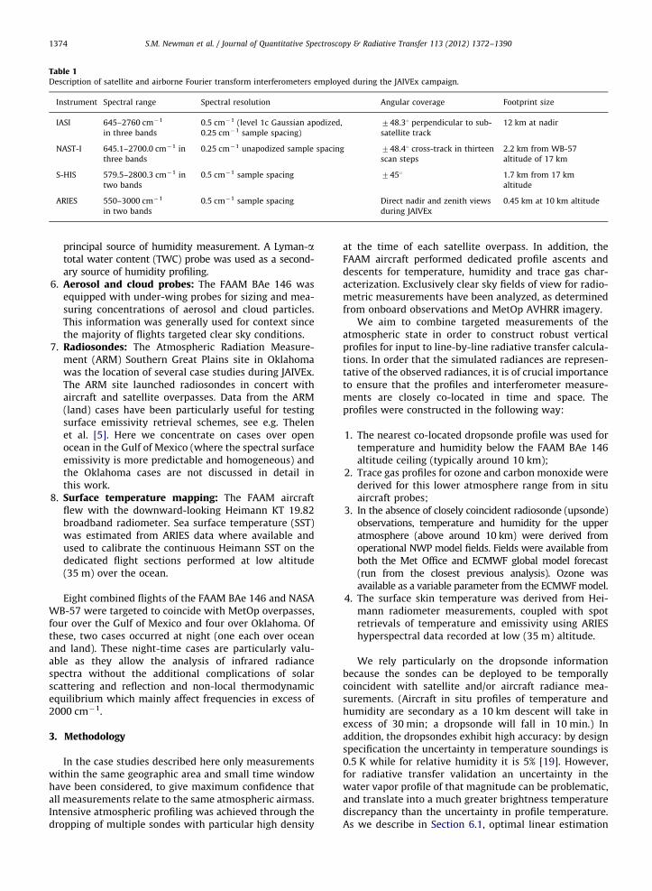

Table 1Description of satellite and airborne Fourier transform interferometers employed during the JAIVEx campaign.

Instrument Spectral range Spectral resolution Angular coverage Footprint size

IASI 645–2760 cm�1

in three bands

0.5 cm�1 (level 1c Gaussian apodized,

0.25 cm�1 sample spacing)

748.31 perpendicular to sub-

satellite track

12 km at nadir

NAST-I 645.1–2700.0 cm�1 in

three bands

0.25 cm�1 unapodized sample spacing 748.41 cross-track in thirteen

scan steps

2.2 km from WB-57

altitude of 17 km

S-HIS 579.5–2800.3 cm�1 in

two bands

0.5 cm�1 sample spacing 7451 1.7 km from 17 km

altitude

ARIES 550–3000 cm�1

in two bands

0.5 cm�1 sample spacing Direct nadir and zenith views

during JAIVEx

0.45 km at 10 km altitude

S.M. Newman et al. / Journal of Quantitative Spectroscopy & Radiative Transfer 113 (2012) 1372–13901374

principal source of humidity measurement. A Lyman-atotal water content (TWC) probe was used as a second-ary source of humidity profiling.

6.

Aerosol and cloud probes: The FAAM BAe 146 wasequipped with under-wing probes for sizing and mea-suring concentrations of aerosol and cloud particles.This information was generally used for context sincethe majority of flights targeted clear sky conditions.

7.

Radiosondes: The Atmospheric Radiation Measure-ment (ARM) Southern Great Plains site in Oklahomawas the location of several case studies during JAIVEx.The ARM site launched radiosondes in concert withaircraft and satellite overpasses. Data from the ARM(land) cases have been particularly useful for testingsurface emissivity retrieval schemes, see e.g. Thelenet al. [5]. Here we concentrate on cases over openocean in the Gulf of Mexico (where the spectral surfaceemissivity is more predictable and homogeneous) andthe Oklahoma cases are not discussed in detail inthis work.

8.

Surface temperature mapping: The FAAM aircraftflew with the downward-looking Heimann KT 19.82broadband radiometer. Sea surface temperature (SST)was estimated from ARIES data where available andused to calibrate the continuous Heimann SST on thededicated flight sections performed at low altitude(35 m) over the ocean.

Eight combined flights of the FAAM BAe 146 and NASAWB-57 were targeted to coincide with MetOp overpasses,four over the Gulf of Mexico and four over Oklahoma. Ofthese, two cases occurred at night (one each over oceanand land). These night-time cases are particularly valu-able as they allow the analysis of infrared radiancespectra without the additional complications of solarscattering and reflection and non-local thermodynamicequilibrium which mainly affect frequencies in excess of2000 cm�1.

3. Methodology

In the case studies described here only measurementswithin the same geographic area and small time windowhave been considered, to give maximum confidence thatall measurements relate to the same atmospheric airmass.Intensive atmospheric profiling was achieved through thedropping of multiple sondes with particular high density

at the time of each satellite overpass. In addition, theFAAM aircraft performed dedicated profile ascents anddescents for temperature, humidity and trace gas char-acterization. Exclusively clear sky fields of view for radio-metric measurements have been analyzed, as determinedfrom onboard observations and MetOp AVHRR imagery.

We aim to combine targeted measurements of theatmospheric state in order to construct robust verticalprofiles for input to line-by-line radiative transfer calcula-tions. In order that the simulated radiances are represen-tative of the observed radiances, it is of crucial importanceto ensure that the profiles and interferometer measure-ments are closely co-located in time and space. Theprofiles were constructed in the following way:

1.

The nearest co-located dropsonde profile was used fortemperature and humidity below the FAAM BAe 146altitude ceiling (typically around 10 km);

2.

Trace gas profiles for ozone and carbon monoxide werederived for this lower atmosphere range from in situaircraft probes;

3.

In the absence of closely coincident radiosonde (upsonde)observations, temperature and humidity for the upperatmosphere (above around 10 km) were derived fromoperational NWP model fields. Fields were available fromboth the Met Office and ECMWF global model forecast(run from the closest previous analysis). Ozone wasavailable as a variable parameter from the ECMWF model.

4.

The surface skin temperature was derived from Hei-mann radiometer measurements, coupled with spotretrievals of temperature and emissivity using ARIEShyperspectral data recorded at low (35 m) altitude.

We rely particularly on the dropsonde informationbecause the sondes can be deployed to be temporally

coincident with satellite and/or aircraft radiance mea-surements. (Aircraft in situ profiles of temperature andhumidity are secondary as a 10 km descent will take inexcess of 30 min; a dropsonde will fall in 10 min.) Inaddition, the dropsondes exhibit high accuracy: by designspecification the uncertainty in temperature soundings is0.5 K while for relative humidity it is 5% [19]. However,for radiative transfer validation an uncertainty in thewater vapor profile of that magnitude can be problematic,and translate into a much greater brightness temperaturediscrepancy than the uncertainty in profile temperature.As we describe in Section 6.1, optimal linear estimation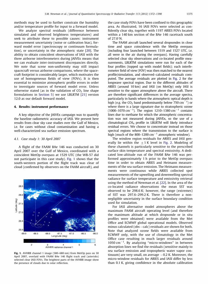

S.M. Newman et al. / Journal of Quantitative Spectroscopy & Radiative Transfer 113 (2012) 1372–1390 1375

methods may be used to further constrain the humidityand/or temperature profile for input to a forward model.

We analyze spectral residuals (difference betweensimulated and observed brightness temperatures) andseek to attribute these to possible causes: instrumentmeasurement uncertainty (noise or calibration bias), for-ward model error (spectroscopy or continuum formula-tion), or uncertainty in the atmospheric state [20]. Theability to obtain coincident observations of IASI with thethree airborne interferometers during JAIVEx means thatwe can evaluate inter-instrument discrepancies directly.We note that scene non-uniformity may still impactspacecraft versus airborne comparisons, where the space-craft footprint is considerably larger, which motivates theuse of homogeneous fields of view (FOVs). It is thenessential to minimize atmospheric profile errors in orderto investigate sources of forward model error. Unlessotherwise stated (as in the validation of CO2 line shapeformulations in Section 5) we use LBLRTM [21] version12.0 as our default forward model.

4. Results: instrument performance

A key objective of the JAIVEx campaign was to quantifythe baseline radiometric accuracy of IASI. We present hereresults from clear sky case studies over the Gulf of Mexico,i.e. for cases without cloud contamination and having awell-characterized sea surface emission spectrum.

4.1. Case study 1: 30 April 2007

A flight of the FAAM BAe 146 was conducted on 30April 2007 over the Gulf of Mexico, coordinated with acoincident MetOp overpass at 1529 UTC (the WB-57 didnot participate in this case study). Fig. 1 shows that thesouth-western portion of the flight track was clear ofcloud (confirmed by observers on the FAAM aircraft), and

Fig. 1. AVHRR channel 1 image (580–680 nm) from MetOp pass on 30

April 2007, overlaid with FAAM BAe 146 flight track and (asterisks)

selected clear IASI FOVs. The brightest parts of the AVHRR image show

the presence of clouds due to solar reflection.

the case study FOVs have been confined to this geographicarea. As illustrated, 16 IASI FOVs were selected as con-fidently clear sky, together with 1197 ARIES FOVs locatedwithin a 140 km section of the BAe 146 racetrack southof 27.01N.

The FAAM aircraft launched several dropsondes in closetime and space coincidence with the MetOp overpass(including four launched between 1519 and 1527 UTC, i.e.all were in the air during the overpass). Having carefullyselected clear sky observations and co-located profile mea-surements, LBLRTM simulations were run for each of thefour profiles (topped up with model fields); each interfe-rometer field of view (FOV) was then matched to the nearestprofile/simulation, and observed–calculated residuals com-puted. The average residuals are plotted in Fig. 2 for thelongwave spectral region. Due to the different altitudes ofARIES (around 10 km) and IASI (on MetOp) only IASI issensitive to the upper atmosphere above the aircraft. Thereare therefore significant differences in the average spectra,particularly in bands where the atmospheric optical depth ishigh (e.g. the CO2 band predominantly below 750 cm�1) orwhere there is a large signature due to stratospheric ozone(1000–1070 cm�1). The region 1210–1380 cm�1 containslines due to methane for which the atmospheric concentra-tion was not measured during JAIVEx, so the use of aclimatological CH4 profile in LBLRTM will likely introduceresidual errors. We choose to concentrate instead on thosespectral regions where the transmission to the surface ishigh (much of the 800–1200 cm�1 atmospheric window).

The window region residuals for ARIES and IASI gen-erally lie within the 71 K level in Fig. 2. Modeling ofthese channels is particularly sensitive to the prescribedsurface skin temperature and spectral emissivity. A dedi-cated low-altitude run of the FAAM BAe 146 was per-formed approximately 1 h prior to the MetOp overpasstime in order to obtain ARIES and Heimann measure-ments of the sea surface emission. The Heimann measure-ments were continuous while ARIES collected spotmeasurements of the upwelling and downwelling spectralradiance for surface temperature and emissivity retrievalusing the method of Newman et al. [22]. In the area of theco-located radiance observations the mean SST wasobserved to be 298.6 K; however, the range (extremes)of SST was 297.6–299.2 K. There is therefore a non-negligible uncertainty in the surface boundary conditionused for simulation.

For IASI alternative model atmospheres above themaximum FAAM aircraft operating level (and thereforethe maximum altitude at which dropsonde or in situprofiles were obtained) were available from the MetOffice and ECMWF global operational models. Observedminus calculated (obs�calc) residuals are shown for both.Note that analyzed ozone fields were available fromECMWF only, with the use of climatology in the MetOffice case resulting in much larger residuals around1050 cm�1. By analyzing ‘‘micro-windows’’ in betweenabsorption lines we find the residuals (sensitive mainly tosea surface emission and tropospheric water vapor con-tinuum) are very small, on average �0.2 K. Moreover, themicro-window residuals for ARIES and IASI differ by lessthan 0.1 K, giving confidence in the absolute calibration

600 700 800 900 1000 1100 1200 1300 1400210220230240250260270280290300

Bri

ghtn

ess

tem

pera

ture

(K

)

IASI spectrum

ARIES spectrum

600 700 800 900 1000 1100 1200 1300 1400Wavenumber (cm-1)

-3-2-10123456

Obs

-cal

c re

sidu

al (

K) IASI obs-calc (EC model)

IASI obs-calc (MO model)ARIES obs-calc

Fig. 2. Comparison of IASI and ARIES co-located nadir-viewing spectra from 30 April 2007. The spectra are averages of clear sky fields of view only. Upper

plot: brightness temperature spectra of IASI and ARIES. Lower plot: residual differences between observations and LBLRTM simulations where the nearest

dropsonde has been used as the model profile. In the case of IASI the model upper atmosphere profile was initialized separately with Met Office (MO) and

ECMWF (EC) NWP fields. The IASI data are Level 1c apodized while the ARIES data are unapodized.

S.M. Newman et al. / Journal of Quantitative Spectroscopy & Radiative Transfer 113 (2012) 1372–13901376

accuracy. It is likely that the �0.2 K residual offsetobserved for both instruments is due to small spatial ortemporal variability in SST not captured during the low-altitude ARIES measurements from which the model-input SST was derived.

4.2. Case study 2: 29 April 2007

The second case study discussed here concerns acoordinated FAAM BAe 146 and WB-57 flight on 29 April2007, conducted over the Gulf of Mexico with a MetOpoverpass at 1550 UTC. The northern portion of the flighttrack was clear of cloud, and again the case study instru-ment FOVs have been confined to this geographic area.Dropsondes were launched at 1531 and 1540 UTC in closeproximity to the overpass time. Since the two aircraft andMetOp operate at different altitudes, their respectiveinterferometers are sensitive to different parts of theatmosphere, at least over those spectral regions withtransmittances significantly less than unity. However, aswith the 30 April case study, by analyzing micro-windowsit is possible to compare directly radiances from the fourinstruments to test their respective calibration accuracies.Note that the satellite zenith angle for the IASI footprintsdoes not exceed 2.61 for the selected FOVs, so it islegitimate to compare these data with directly upwellingradiances recorded by the other interferometers.

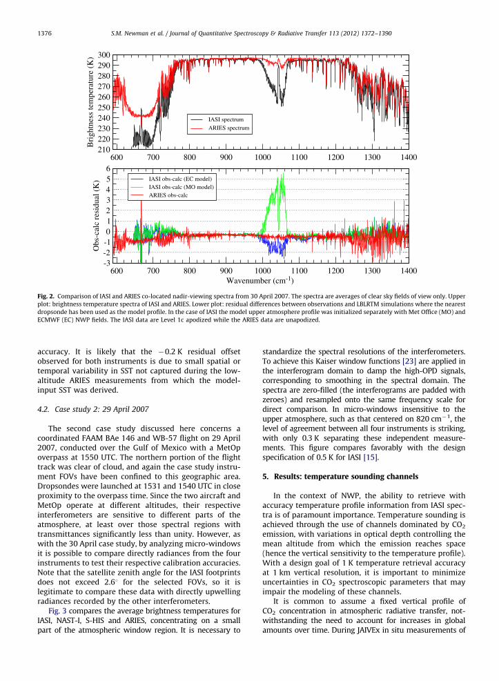
Fig. 3 compares the average brightness temperatures forIASI, NAST-I, S-HIS and ARIES, concentrating on a smallpart of the atmospheric window region. It is necessary to

standardize the spectral resolutions of the interferometers.To achieve this Kaiser window functions [23] are applied inthe interferogram domain to damp the high-OPD signals,corresponding to smoothing in the spectral domain. Thespectra are zero-filled (the interferograms are padded withzeroes) and resampled onto the same frequency scale fordirect comparison. In micro-windows insensitive to theupper atmosphere, such as that centered on 820 cm�1, thelevel of agreement between all four instruments is striking,with only 0.3 K separating these independent measure-ments. This figure compares favorably with the designspecification of 0.5 K for IASI [15].

5. Results: temperature sounding channels

In the context of NWP, the ability to retrieve withaccuracy temperature profile information from IASI spec-tra is of paramount importance. Temperature sounding isachieved through the use of channels dominated by CO2

emission, with variations in optical depth controlling themean altitude from which the emission reaches space(hence the vertical sensitivity to the temperature profile).With a design goal of 1 K temperature retrieval accuracyat 1 km vertical resolution, it is important to minimizeuncertainties in CO2 spectroscopic parameters that mayimpair the modeling of these channels.

It is common to assume a fixed vertical profile ofCO2 concentration in atmospheric radiative transfer, not-withstanding the need to account for increases in globalamounts over time. During JAIVEx in situ measurements of

805 810 815 820 825 830

Wavenumber (1/cm)

291

292

293

294

295

Bri

ghtn

ess

tem

pera

ture

(K

)

IASI

ARIES

S-HIS

NAST-I

JAIVEx case studyAt comparable spectral resolutions

Fig. 3. Comparison of spatially- and temporally-coincident brightness temperatures from the four interferometers studied during JAIVEx, focussing on

part of the atmospheric window spectral region. The respective spectral resolutions of the data have been degraded to standardize the brightness

temperatures and enable a direct comparison. The micro-window around 817–823 cm�1 has been analyzed to quantify inter-spectrometer agreement, as

described in the text.

S.M. Newman et al. / Journal of Quantitative Spectroscopy & Radiative Transfer 113 (2012) 1372–1390 1377

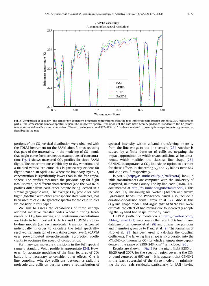
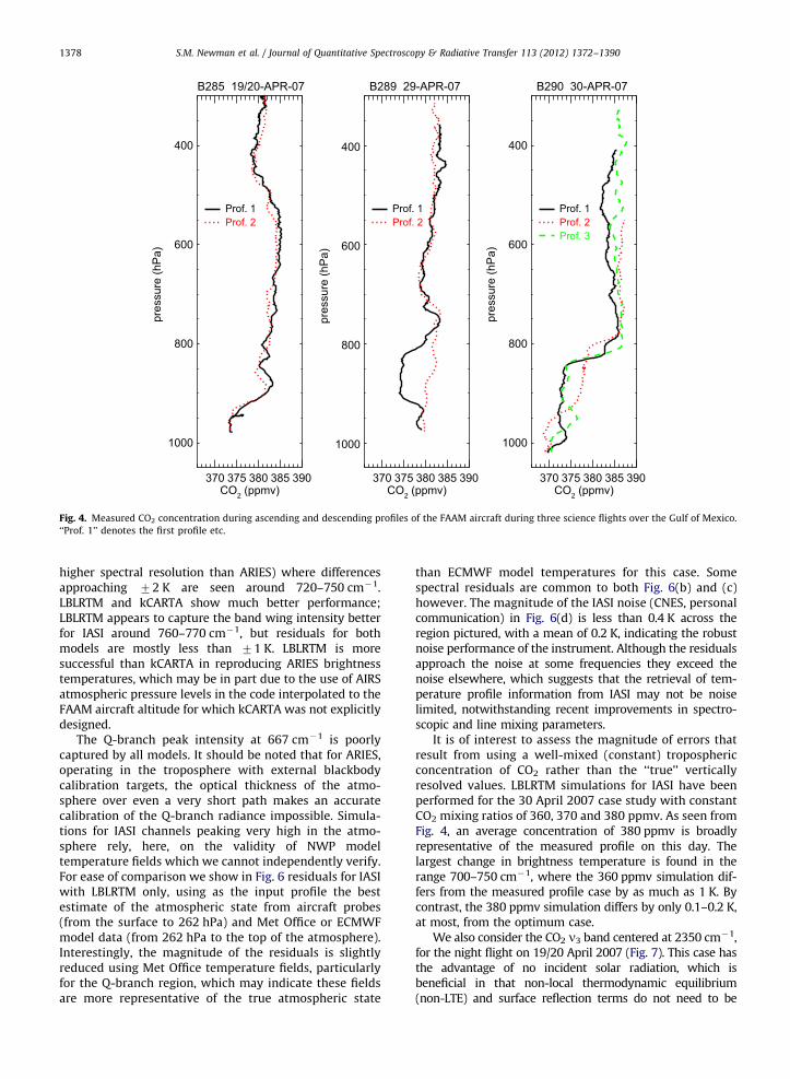
portions of the CO2 vertical distribution were obtained withthe TDLAS instrument on the FAAM aircraft, thus reducingthat part of the uncertainty in the modeling of CO2 bandsthat might come from erroneous assumptions of concentra-tion. Fig. 4 shows measured CO2 profiles for three FAAMflights. The concentrations exhibit day-to-day variations anda marked vertical structure, this is particularly evident forflight B290 on 30 April 2007 where the boundary layer CO2

concentration is significantly lower than in the free tropo-sphere. The profiles measured the previous day for flightB289 show quite different characteristics (and the two B289profiles differ from each other despite being located in asimilar geographic area). The average CO2 profile for eachflight (together with other atmospheric state variables) hasbeen used to calculate synthetic spectra for the case studieswe consider in this paper.

We aim to assess the capabilities of three widely-adopted radiative transfer codes where differing treat-ments of CO2 line mixing and continuum contributionsare likely to be important. GENLN2 and LBLRTM are line-by-line models (i.e. each molecular transition is treatedindividually in order to calculate the total spectrally-resolved transmission of each atmospheric layer). kCARTAuses pre-computed monochromatic absorption coeffi-cients to optimize the speed of computation.

For many gas molecule transitions in the IASI spectralrange a standard Voigt profile is appropriate [24]. How-ever, for accurate modeling of the finer features of CO2

bands it is necessary to consider other effects. One isline coupling, whereby collisions between a radiatingmolecule and collision partner cause a redistribution of

spectral intensity within a band, transferring intensityfrom the line wings to the line centers [25]. Another iscaused by a finite duration of collision, negating theimpact approximation which treats collisions as instanta-neous, which modifies the classical line shape [26].GENLN2 incorporates a CO2 line shape option to accountfor these effects in the strong n2 and n3 bands near 667and 2385 cm�1 respectively.

kCARTA (http://asl.umbc.edu/pub/rta/kcarta) look-uptable transmittances are computed with the University ofMaryland, Baltimore County line-by-line code (UMBC-LBL,documented at http://asl.umbc.edu/pub/rta/umbclbl/). Thisincludes CO2 line-mixing for twelve Q-branch and twelveP/R-branch bands; the P/R-branch bands also include aduration-of-collision term. Strow et al. [27] discuss thisCO2 line shape model, and argue that GENLN2 will over-estimate the effect of line mixing due to incorrectly adopt-ing the n3 band line shape for the n2 band.

LBLRTM (with documentation at http://rtweb.aer.com/lblrtm_frame.html) incorporates the recent CO2 line mixingdatabase of Lamouroux et al. [28] and utilizes line positionsand intensities given by to Flaud et al. [9]. The formalism ofNiro et al. [29] has been used to calculate the couplingcoefficients. The far-wing line shape is incorporated into theMT_CKD continuum for CO2 for which a temperature depen-dence in the range of 2386–2434 cm�1 is included [30].

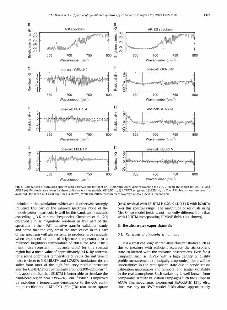
Results are shown in Fig. 5 for the night flight B285 on19/20 April 2007, for the spectral region covering the CO2

n2 band centered at 667 cm�1. It is apparent that GENLN2is the least successful of the three models in minimiz-ing the obs�calc residuals, particularly for IASI (having

B285 19/20-APR-07

370 375 380 385 390CO2 (ppmv)

1000

800

600

400pr

essu

re (h

Pa)

Prof. 1Prof. 2

B289 29-APR-07

370 375 380 385 390CO2 (ppmv)

1000

800

600

400

pres

sure

(hP

a)

Prof. 1Prof. 2

B290 30-APR-07

370 375 380 385 390CO2 (ppmv)

1000

800

600

400

pres

sure

(hP

a)

Prof. 1Prof. 2Prof. 3

Fig. 4. Measured CO2 concentration during ascending and descending profiles of the FAAM aircraft during three science flights over the Gulf of Mexico.

‘‘Prof. 1’’ denotes the first profile etc.

S.M. Newman et al. / Journal of Quantitative Spectroscopy & Radiative Transfer 113 (2012) 1372–13901378

higher spectral resolution than ARIES) where differencesapproaching 72 K are seen around 720–750 cm�1.LBLRTM and kCARTA show much better performance;LBLRTM appears to capture the band wing intensity betterfor IASI around 760–770 cm�1, but residuals for bothmodels are mostly less than 71 K. LBLRTM is moresuccessful than kCARTA in reproducing ARIES brightnesstemperatures, which may be in part due to the use of AIRSatmospheric pressure levels in the code interpolated to theFAAM aircraft altitude for which kCARTA was not explicitlydesigned.

The Q-branch peak intensity at 667 cm�1 is poorlycaptured by all models. It should be noted that for ARIES,operating in the troposphere with external blackbodycalibration targets, the optical thickness of the atmo-sphere over even a very short path makes an accuratecalibration of the Q-branch radiance impossible. Simula-tions for IASI channels peaking very high in the atmo-sphere rely, here, on the validity of NWP modeltemperature fields which we cannot independently verify.For ease of comparison we show in Fig. 6 residuals for IASIwith LBLRTM only, using as the input profile the bestestimate of the atmospheric state from aircraft probes(from the surface to 262 hPa) and Met Office or ECMWFmodel data (from 262 hPa to the top of the atmosphere).Interestingly, the magnitude of the residuals is slightlyreduced using Met Office temperature fields, particularlyfor the Q-branch region, which may indicate these fieldsare more representative of the true atmospheric state

than ECMWF model temperatures for this case. Somespectral residuals are common to both Fig. 6(b) and (c)however. The magnitude of the IASI noise (CNES, personalcommunication) in Fig. 6(d) is less than 0.4 K across theregion pictured, with a mean of 0.2 K, indicating the robustnoise performance of the instrument. Although the residualsapproach the noise at some frequencies they exceed thenoise elsewhere, which suggests that the retrieval of tem-perature profile information from IASI may not be noiselimited, notwithstanding recent improvements in spectro-scopic and line mixing parameters.

It is of interest to assess the magnitude of errors thatresult from using a well-mixed (constant) troposphericconcentration of CO2 rather than the ‘‘true’’ verticallyresolved values. LBLRTM simulations for IASI have beenperformed for the 30 April 2007 case study with constantCO2 mixing ratios of 360, 370 and 380 ppmv. As seen fromFig. 4, an average concentration of 380 ppmv is broadlyrepresentative of the measured profile on this day. Thelargest change in brightness temperature is found in therange 700–750 cm�1, where the 360 ppmv simulation dif-fers from the measured profile case by as much as 1 K. Bycontrast, the 380 ppmv simulation differs by only 0.1–0.2 K,at most, from the optimum case.

We also consider the CO2 n3 band centered at 2350 cm�1,for the night flight on 19/20 April 2007 (Fig. 7). This case hasthe advantage of no incident solar radiation, which isbeneficial in that non-local thermodynamic equilibrium(non-LTE) and surface reflection terms do not need to be

650 700 750 800Wavenumber (cm-1)

200220240260280300

Brig

htne

ss te

mp.

(K)

650 700 750 800Wavenumber (cm-1)

220240260280300

Brig

htne

ss te

mp.

(K)

650 700 750 800Wavenumber (cm-1)

-4-3-2-1012

Res

idua

l (K

)

650 700 750 800Wavenumber (cm-1)

-3-2-10123

Res

idua

l (K

)

650 700 750 800Wavenumber (cm-1)

-4-3-2-1012

Res

idua

l (K

)

650 700 750 800Wavenumber (cm-1)

-3-2-10123

Res

idua

l (K

)

650 700 750 800Wavenumber (cm-1)

-4-3-2-1012

Res

idua

l (K

)

650 700 750 800Wavenumber (cm-1)

-3-2-10123

Res

idua

l (K

)

IASI spectrum ARIES spectrum

obs-calc GENLN2 obs-calc GENLN2

obs-calc kCARTA obs-calc kCARTA

obs-calc LBLRTM obs-calc LBLRTM

Fig. 5. Comparison of simulated spectra with observations for flight on 19/20 April 2007. Spectra covering the CO2 n2 band are shown for IASI, (a) and

ARIES, (e). Residuals are shown for three radiative transfer models: GENLN2 (b, f), kCARTA (c, g) and LBLRTM (d, h). The IASI observations are Level 1c

apodized (the mean of 4 clear sky FOVs is shown) while the ARIES measurement (average of 357 FOVs) is unapodized.

S.M. Newman et al. / Journal of Quantitative Spectroscopy & Radiative Transfer 113 (2012) 1372–1390 1379

included in the calculations which would otherwise stronglyinfluence this part of the infrared spectrum. None of themodels perform particularly well for this band, with residualsexceeding 73 K at some frequencies. Shephard et al. [20]observed similar magnitude residuals in this part of thespectrum in their IASI radiative transfer validation studyand noted that the very small radiance values in this partof the spectrum will always tend to produce large residualswhen expressed in units of brightness temperature. At areference brightness temperature of 280 K the IASI instru-ment noise (constant in radiance units) for this spectralregion has a mean value of approximately 0.4 K. By contrast,for a scene brightness temperature of 220 K the instrumentnoise is closer to 5 K. LBLRTM and kCARTA simulations do notsuffer from most of the high-frequency residual structureseen for GENLN2, most particularly around 2200–2250 cm�1.It is apparent also that LBLRTM is better able to simulate theband-head region near 2395–2435 cm�1 which is improvedby including a temperature dependence to the CO2 conti-nuum coefficients in MT_CKD [30]. (The root mean square

(rms) residual with LBLRTM is 0.23 K c.f. 0.31 K with kCARTAover this spectral range.) The magnitude of residuals usingMet Office model fields is not markedly different from thatwith LBLRTM incorporating ECMWF fields (not shown).

6. Results: water vapor channels

6.1. Retrievals of atmospheric humidity

It is a great challenge in ‘‘radiative closure’’ studies such asthis to measure with sufficient accuracy the atmosphericstate co-located with the radiance observations. Even for acampaign such as JAIVEx with a high density of qualityprofile measurements (principally dropsondes) there will beuncertainties in the atmospheric state due to sonde sensorcalibration inaccuracies and temporal and spatial variabilityin the real atmosphere. Such variability is well known fromcomparable satellite validation campaigns such the EuropeanAQUA Thermodynamic Experiment (EAQUATE) [31]. Also,since we rely on NWP model fields above approximately

650 700 750 800Wavenumber (cm-1)

200220240260280300

Brig

htne

ss te

mp.

(K)

650 700 750 800Wavenumber (cm-1)

-3-2-101

Res

idua

l (K

)

650 700 750 800Wavenumber (cm-1)

-3-2-101

Res

idua

l (K

)

650 700 750 800Wavenumber (cm-1)

-3-2-101

Brig

htne

ss te

mp.

(K)

IASI spectrum

obs-calc LBLRTM (EC upper atm.)

obs-calc LBLRTM (MO upper atm.)

IASI instrument noise

Fig. 6. Comparison of simulated spectra for IASI (a) covering the CO2 n2

band, where the residual plot (b) is the same as Fig. 5(d) with the

LBLRTM vertical profile above the maximum aircraft altitude taken from

ECMWF model fields. Residuals are shown in (c) with the upper atmo-

sphere derived from the Met Office model state. Confidence bounds

representing the (7) IASI instrument noise are shown in (d).

2150 2200 2250 2300 2350 2400 2450 2500Wavenumber (cm-1)

200220240260280300

Brig

htne

ss te

mp.

(K)

2150 2200 2250 2300 2350 2400 2450 2500Wavenumber (cm-1)

-4-3-2-1012

Res

idua

l (K

)

2150 2200 2250 2300 2350 2400 2450 2500Wavenumber (cm-1)

-4-3-2-1012

Res

idua

l (K

)

2150 2200 2250 2300 2350 2400 2450 2500Wavenumber (cm-1)

-4-3-2-1012

Res

idua

l (K

)

IASI spectrum

obs-calc GENLN2

obs-calc kCARTA

obs-calc LBLRTM

Fig. 7. As Fig. 5(a)–(d) covering the CO2 n3 band for IASI.

S.M. Newman et al. / Journal of Quantitative Spectroscopy & Radiative Transfer 113 (2012) 1372–13901380

10 km altitude, we particularly have uncertainties in uppertropospheric–lower stratospheric (UTLS) humidity for theJAIVEx case studies. It has been demonstrated [32] that UTLShumidity fields from different NWP centers can be consider-ably at variance. One solution is to use supplementarymeasurements such as ground-based microwave radiometersto constrain the sonde-derived atmospheric profile [33].Alternatively, the high information content in hyperspectralradiance observations may permit the retrieval of atmo-spheric state parameters where the accuracy of the profilemeasurements is a limiting factor [20].

During JAIVEx the Microwave Airborne Radiometer Scan-ning System (MARSS) was flown on the FAAM BAe 146 onall sorties. MARSS [34] operates at the same frequencies asthe Advanced Microwave Sounding Unit (AMSU-B) on theNational Oceanic and Atmospheric Administration polarorbiting satellites, except the 150 GHz channel is replaced

with 157 GHz as for MHS. The channels are numberedfollowing the AMSU nomenclature from 16 to 20, centeredat 89, 157, 18371, 18373 and 18377 GHz. The dual-passband 183 GHz channels are located in the region of awater vapor absorption line but sensitive to different parts ofthe atmosphere. Thus, when operating at relatively highaltitude (in the upper troposphere) and viewing upwards,MARSS is sensitive to UTLS water vapor and can be used toretrieve more accurate profiles than are available from modelfields alone. During JAIVEx the 89 GHz channel was notserviceable while the data quality from 157 GHz was poor;therefore only the 183 GHz channels are considered here.

We can also make use of satellite microwave sound-ings from the Microwave Humidity Sounder (MHS) car-ried on MetOp and, along with IASI, underflown duringJAIVEx. MHS [35] is sensitive to similar spectral bands asMARSS and AMSU-B. The nadir viewing MHS observationsare complementary to the zenith views of MARSS, withsensitivity via their weighting functions to different partsof the atmosphere. The microwave effective sea surfacetemperature is assumed to be the same as used in theinfrared; for microwave sea surface emissivity we adopt

S.M. Newman et al. / Journal of Quantitative Spectroscopy & Radiative Transfer 113 (2012) 1372–1390 1381

values consistent with low-altitude MARSS observationsduring JAIVEx (C. Harlow, personal communication).

Optimal linear estimation methods have found wideapplication in the fields of ground-based microwaveretrievals [36] and NWP radiance assimilation [37], andhave been used successfully in the retrieval of atmo-spheric profiles, cloud properties and surface parametersfrom IASI spectra during JAIVEx [38]. Following Rodgers [39]we can calculate

xiþ1 ¼ xaþðHT R�1HþB�1

Þ�1HT R�1

½y�FðxiÞþHðxi�xaÞ�

ð1Þ

where xiþ1 is the state vector containing quantities such asvertical profiles of temperature and humidity after iþ1iterations, xa is the prior estimate of the state (the back-ground), y is the vector of observed radiances, F is theforward radiative transfer model, H contains the Jacobians(derivatives of forward modeled radiances with respect to x),R is the observation error covariance matrix (representinginstrument and radiative transfer error) and B is the back-ground error covariance matrix. We use MonoRTM [21] asthe code for forward modeling and Jacobian computation inthe microwave.

We adopt the methodology of Haefele and Kampfer [36]by constructing B matrix error covariances in terms ofstandard deviations s for each atmospheric layer with avertical correlation length of 1.5 km. Where we have drop-sonde information, s is based on an uncertainty of 5% inrelative humidity for RD93 dropsondes [19] while for higheraltitude layers s is taken from the ECMWF B matrixdiagonal terms (s2). Due to limited temperature informa-tion in the 183 GHz measurements only water vaporamount is allowed to vary in the retrieval, with thetemperature profile fixed (composite from dropsonde andECMWF upper atmosphere).

To construct our observation error matrix we assume astandard deviation for all 183 GHz channels (MARSS andMHS) of 2.5 K, i.e. for uncorrelated errors the matrix isdiagonal with variances along the diagonal of 6.25K2. Theseobservation errors are significantly higher than purelyinstrumental noise would suggest; for MARSS [40] andMHS [41] the 183 GHz channels exhibit an rms accuracytypically less than 1 K. However, we find that it is impos-sible to fit to observations with such restrictive errors andneed to relax this constraint to achieve a reliable retrieval.

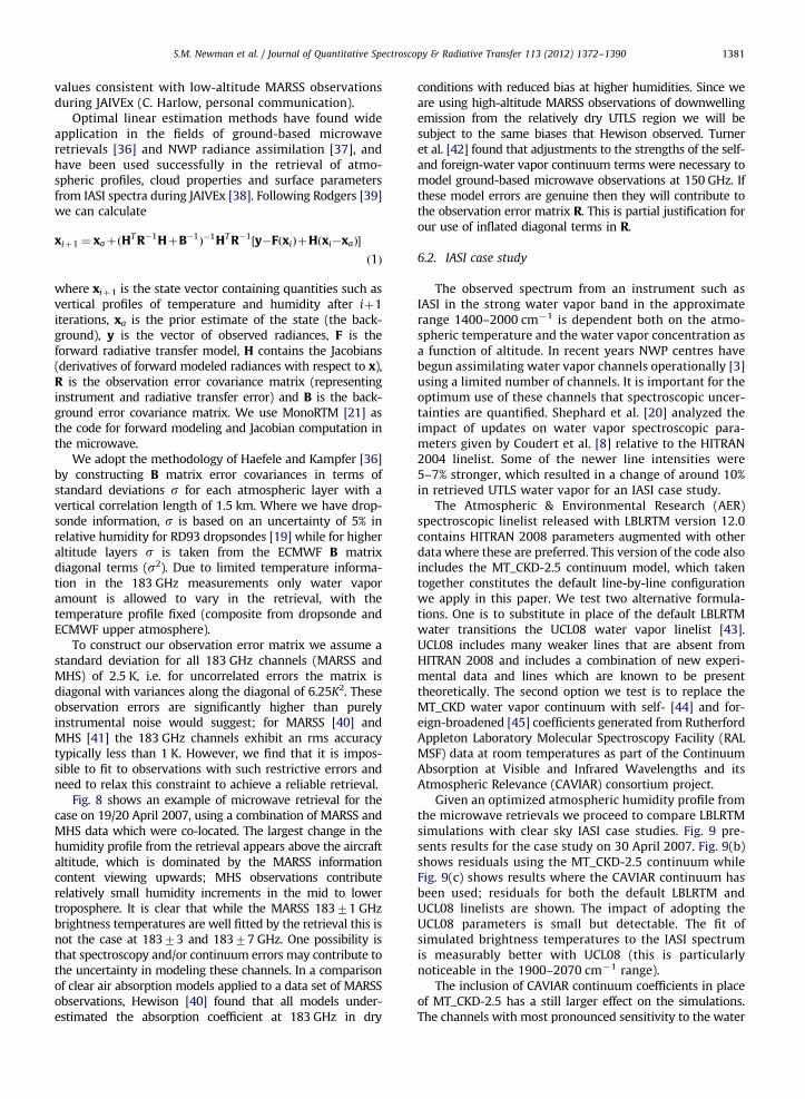
Fig. 8 shows an example of microwave retrieval for thecase on 19/20 April 2007, using a combination of MARSS andMHS data which were co-located. The largest change in thehumidity profile from the retrieval appears above the aircraftaltitude, which is dominated by the MARSS informationcontent viewing upwards; MHS observations contributerelatively small humidity increments in the mid to lowertroposphere. It is clear that while the MARSS 18371 GHzbrightness temperatures are well fitted by the retrieval this isnot the case at 18373 and 18377 GHz. One possibility isthat spectroscopy and/or continuum errors may contribute tothe uncertainty in modeling these channels. In a comparisonof clear air absorption models applied to a data set of MARSSobservations, Hewison [40] found that all models under-estimated the absorption coefficient at 183 GHz in dry

conditions with reduced bias at higher humidities. Since weare using high-altitude MARSS observations of downwellingemission from the relatively dry UTLS region we will besubject to the same biases that Hewison observed. Turneret al. [42] found that adjustments to the strengths of the self-and foreign-water vapor continuum terms were necessary tomodel ground-based microwave observations at 150 GHz. Ifthese model errors are genuine then they will contribute tothe observation error matrix R. This is partial justification forour use of inflated diagonal terms in R.

6.2. IASI case study

The observed spectrum from an instrument such asIASI in the strong water vapor band in the approximaterange 1400–2000 cm�1 is dependent both on the atmo-spheric temperature and the water vapor concentration asa function of altitude. In recent years NWP centres havebegun assimilating water vapor channels operationally [3]using a limited number of channels. It is important for theoptimum use of these channels that spectroscopic uncer-tainties are quantified. Shephard et al. [20] analyzed theimpact of updates on water vapor spectroscopic para-meters given by Coudert et al. [8] relative to the HITRAN2004 linelist. Some of the newer line intensities were5–7% stronger, which resulted in a change of around 10%in retrieved UTLS water vapor for an IASI case study.

The Atmospheric & Environmental Research (AER)spectroscopic linelist released with LBLRTM version 12.0contains HITRAN 2008 parameters augmented with otherdata where these are preferred. This version of the code alsoincludes the MT_CKD-2.5 continuum model, which takentogether constitutes the default line-by-line configurationwe apply in this paper. We test two alternative formula-tions. One is to substitute in place of the default LBLRTMwater transitions the UCL08 water vapor linelist [43].UCL08 includes many weaker lines that are absent fromHITRAN 2008 and includes a combination of new experi-mental data and lines which are known to be presenttheoretically. The second option we test is to replace theMT_CKD water vapor continuum with self- [44] and for-eign-broadened [45] coefficients generated from RutherfordAppleton Laboratory Molecular Spectroscopy Facility (RALMSF) data at room temperatures as part of the ContinuumAbsorption at Visible and Infrared Wavelengths and itsAtmospheric Relevance (CAVIAR) consortium project.

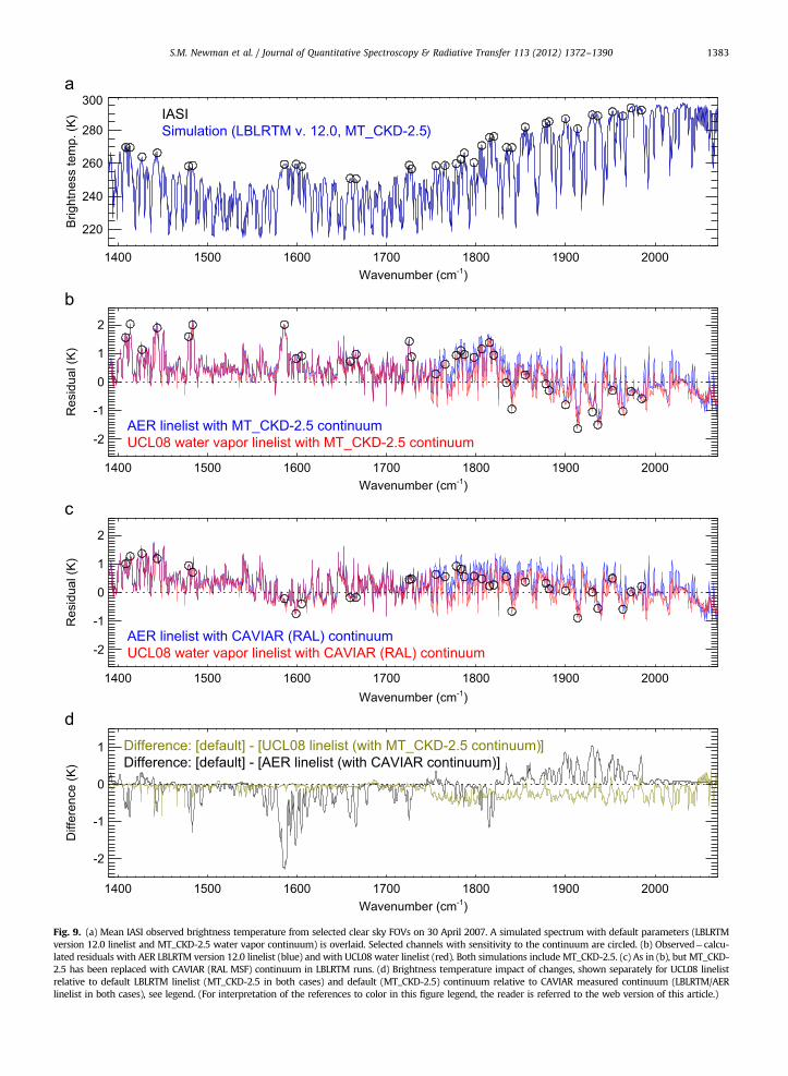
Given an optimized atmospheric humidity profile fromthe microwave retrievals we proceed to compare LBLRTMsimulations with clear sky IASI case studies. Fig. 9 pre-sents results for the case study on 30 April 2007. Fig. 9(b)shows residuals using the MT_CKD-2.5 continuum whileFig. 9(c) shows results where the CAVIAR continuum hasbeen used; residuals for both the default LBLRTM andUCL08 linelists are shown. The impact of adopting theUCL08 parameters is small but detectable. The fit ofsimulated brightness temperatures to the IASI spectrumis measurably better with UCL08 (this is particularlynoticeable in the 1900–2070 cm�1 range).

The inclusion of CAVIAR continuum coefficients in placeof MT_CKD-2.5 has a still larger effect on the simulations.The channels with most pronounced sensitivity to the water

1 10 100 1000 10000VMR (ppmv)

1000

800

600

400

200

p (h

Pa)

BackgroundRetrieval

-10 0 10 20 30 40 50VMR (ppmv)

1000

800

600

400

200

p (h

Pa)

120 140 160 180 200 220angle (deg)

40

45

50

55

60

65

70

75

BT

(K)

MARSS observationsBT from backgroundBT from retrieval

120 140 160 180 200 220angle (deg)

5

10

15

20

BT

(K)

2 3 4 5 6MHS channel

-2

-1

0

1

2

Obs

-mod

el B

T (K

)

Fig. 8. Example of microwave humidity retrieval from case on 19/20 April 2007. (a) Background and retrieved profile of water vapor mixing ratio. The

background was constructed from a combination of dropsonde profile from 318 hPa (this level shown as the horizontal dotted line) down to the surface,

while the upper atmosphere was derived from ECMWF model fields. (b) Retrieval increment in humidity. (c) 18371 GHz and (d) 18373, 18377 GHz

MARSS brightness temperatures measured as a function of view angle (vertically upwards is 1801); circles: MARSS observations, squares: model

brightness temperature from background profile, triangles: model brightness temperature from retrieval. (e) MHS 183 GHz observations minus model

brightness temperatures for background profile (squares) and retrieved profile (triangles).

S.M. Newman et al. / Journal of Quantitative Spectroscopy & Radiative Transfer 113 (2012) 1372–13901382

vapor continuum have been circled in Fig. 9; for most ofthese the CAVIAR continuum coefficients produce smallerresiduals. The smoothness constraints inherent in theMT_CKD formulation make it difficult to reproduce theobserved spectral variation near the band center at1600 cm�1 [20]. By contrast, the CAVIAR coefficients fitthis spectral shape quite well. For the highlighted conti-nuum channels the root mean square (rms) differences arereduced from 1.03 K to 0.58 K. Fig. 9(d) shows the relativebrightness temperature changes produced by the UCL08and CAVIAR spectroscopy/continuum changes. The conti-nuum residual differences are somewhat larger, in excess of2 K at band center.

By analyzing cases for different atmospheric state pro-files, but subject to the same fundamental radiative transfer,we can assign more confidently residual errors to modeldeficiencies rather than simply atmospheric variability.We have repeated the analysis above for the night-time

case on 19/20 April 2007 and find (not shown) a similarpattern of spectral residuals. For this case the rms differ-ences for continuum-sensitive channels are reduced from0.99 K to 0.67 K when CAVIAR continuum coefficients areused instead of MT_CKD.

Examining the residuals in Fig. 9, we observe somedepartures that are still unexplained. It is entirely possiblethat uncertainties remaining in the retrieved verticalprofile contribute to residuals of the order of 71 K. It isalso likely that future improvements in water vaporspectroscopic parameters and continuum coefficients willserve to reduce the residuals further. Shephard et al. [20](see their Fig. 19) discern the signature of water vaporline coupling for two pairs of lines at 1540 cm�1 and1653 cm�1, frequencies at which we also observe rela-tively large residuals. Line coupling is known to be impor-tant for these pairs [46]. New capabilities for calculatingatmospheric line mixing, see e.g. Boone et al. [47] and

1400 1500 1600 1700 1800 1900 2000Wavenumber (cm-1)

220

240

260

280

300

Brig

htne

ss te

mp.

(K) IASI

Simulation (LBLRTM v. 12.0, MT_CKD-2.5)

1400 1500 1600 1700 1800 1900 2000Wavenumber (cm-1)

-2

-1

0

1

2

Res

idua

l (K

)

AER linelist with MT_CKD-2.5 continuumUCL08 water vapor linelist with MT_CKD-2.5 continuum

1400 1500 1600 1700 1800 1900 2000Wavenumber (cm-1)

-2

-1

0

1

2

Res

idua

l (K

)

AER linelist with CAVIAR (RAL) continuumUCL08 water vapor linelist with CAVIAR (RAL) continuum

1400 1500 1600 1700 1800 1900 2000Wavenumber (cm-1)

-2

-1

0

1

Diff

eren

ce (K

) Difference: [default] - [AER linelist (with CAVIAR continuum)]Difference: [default] - [UCL08 linelist (with MT_CKD-2.5 continuum)]

Fig. 9. (a) Mean IASI observed brightness temperature from selected clear sky FOVs on 30 April 2007. A simulated spectrum with default parameters (LBLRTM

version 12.0 linelist and MT_CKD-2.5 water vapor continuum) is overlaid. Selected channels with sensitivity to the continuum are circled. (b) Observed�calcu-

lated residuals with AER LBLRTM version 12.0 linelist (blue) and with UCL08 water linelist (red). Both simulations include MT_CKD-2.5. (c) As in (b), but MT_CKD-

2.5 has been replaced with CAVIAR (RAL MSF) continuum in LBLRTM runs. (d) Brightness temperature impact of changes, shown separately for UCL08 linelist

relative to default LBLRTM linelist (MT_CKD-2.5 in both cases) and default (MT_CKD-2.5) continuum relative to CAVIAR measured continuum (LBLRTM/AER

linelist in both cases), see legend. (For interpretation of the references to color in this figure legend, the reader is referred to the web version of this article.)

S.M. Newman et al. / Journal of Quantitative Spectroscopy & Radiative Transfer 113 (2012) 1372–1390 1383

S.M. Newman et al. / Journal of Quantitative Spectroscopy & Radiative Transfer 113 (2012) 1372–13901384

Tran et al. [48], offer the prospect of including such effectsin line-by-line codes.

6.3. Impact of spectroscopic uncertainties

The HITRAN linelist includes indices which give esti-mated uncertainty ranges for individual parameters (seeTable 5 in Rothman et al. [49]). An uncertainty inwavenumber (cm�1) units is given for line position andair pressure-induced line shift, while a percentage uncer-tainty is specified for line intensity, air- and self-broa-dened half-width and the temperature-dependenceexponent for the air-broadened half-width. The uncer-tainty index is defined within bounds; so, for example, acode 5 for the line intensity gives an estimated uncer-tainty range between Z5% and o10% while a code 6indicates a range of between Z2% and o5%. It should bepossible, therefore, to estimate the likely impact of theseuncertainties on a reference IASI spectrum.

We proceed as follows to generate a set of perturbedparameters within the error bounds specified by theHITRAN 2008 indices. For each parameter for each line arandom number is generated which lies between 0 and 1with uniformly distributed probability. The value of thisnumber determines where in the specified uncertaintyrange the perturbation lies. The perturbation is given arandom sign and added to the default parameter. This isrepeated for all parameters for all water lines in the IASIspectral range, and a modified HITRAN linelist produced.For adequate statistical sampling we generate 100 suchlists, and simulate in Monte Carlo fashion the impact on areference IASI simulation of the spectroscopic changes.

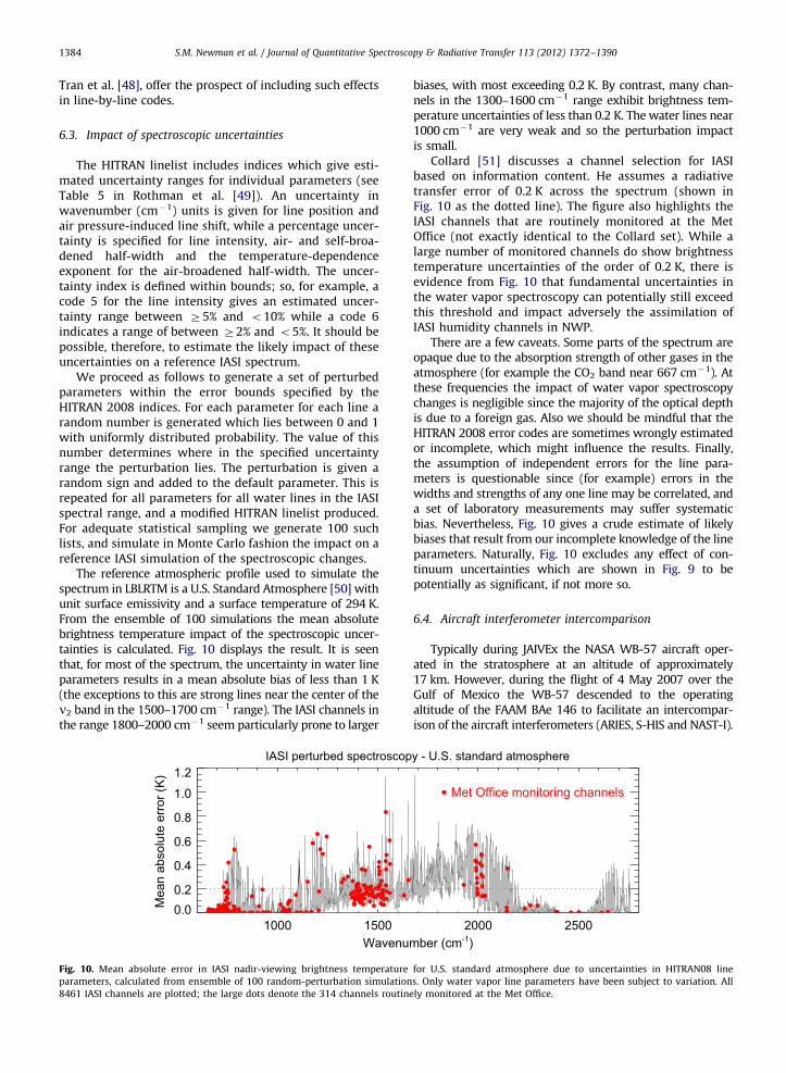
The reference atmospheric profile used to simulate thespectrum in LBLRTM is a U.S. Standard Atmosphere [50] withunit surface emissivity and a surface temperature of 294 K.From the ensemble of 100 simulations the mean absolutebrightness temperature impact of the spectroscopic uncer-tainties is calculated. Fig. 10 displays the result. It is seenthat, for most of the spectrum, the uncertainty in water lineparameters results in a mean absolute bias of less than 1 K(the exceptions to this are strong lines near the center of then2 band in the 1500–1700 cm�1 range). The IASI channels inthe range 1800–2000 cm�1 seem particularly prone to larger

IASI perturbed spectroscop

1000 1500Wavenum

0.00.2

0.4

0.6

0.8

1.0

1.2

Mea

n ab

solu

te e

rror

(K)

Fig. 10. Mean absolute error in IASI nadir-viewing brightness temperature

parameters, calculated from ensemble of 100 random-perturbation simulation

8461 IASI channels are plotted; the large dots denote the 314 channels routine

biases, with most exceeding 0.2 K. By contrast, many chan-nels in the 1300–1600 cm�1 range exhibit brightness tem-perature uncertainties of less than 0.2 K. The water lines near1000 cm�1 are very weak and so the perturbation impactis small.

Collard [51] discusses a channel selection for IASIbased on information content. He assumes a radiativetransfer error of 0.2 K across the spectrum (shown inFig. 10 as the dotted line). The figure also highlights theIASI channels that are routinely monitored at the MetOffice (not exactly identical to the Collard set). While alarge number of monitored channels do show brightnesstemperature uncertainties of the order of 0.2 K, there isevidence from Fig. 10 that fundamental uncertainties inthe water vapor spectroscopy can potentially still exceedthis threshold and impact adversely the assimilation ofIASI humidity channels in NWP.

There are a few caveats. Some parts of the spectrum areopaque due to the absorption strength of other gases in theatmosphere (for example the CO2 band near 667 cm�1). Atthese frequencies the impact of water vapor spectroscopychanges is negligible since the majority of the optical depthis due to a foreign gas. Also we should be mindful that theHITRAN 2008 error codes are sometimes wrongly estimatedor incomplete, which might influence the results. Finally,the assumption of independent errors for the line para-meters is questionable since (for example) errors in thewidths and strengths of any one line may be correlated, anda set of laboratory measurements may suffer systematicbias. Nevertheless, Fig. 10 gives a crude estimate of likelybiases that result from our incomplete knowledge of the lineparameters. Naturally, Fig. 10 excludes any effect of con-tinuum uncertainties which are shown in Fig. 9 to bepotentially as significant, if not more so.

6.4. Aircraft interferometer intercomparison

Typically during JAIVEx the NASA WB-57 aircraft oper-ated in the stratosphere at an altitude of approximately17 km. However, during the flight of 4 May 2007 over theGulf of Mexico the WB-57 descended to the operatingaltitude of the FAAM BAe 146 to facilitate an intercompar-ison of the aircraft interferometers (ARIES, S-HIS and NAST-I).

y - U.S. standard atmosphere

2000 2500ber (cm-1)

Met Office monitoring channels

for U.S. standard atmosphere due to uncertainties in HITRAN08 line

s. Only water vapor line parameters have been subject to variation. All

ly monitored at the Met Office.

S.M. Newman et al. / Journal of Quantitative Spectroscopy & Radiative Transfer 113 (2012) 1372–1390 1385

It was not possible to match the airspeeds of the aircraft, andcarry out a wingtip-to-wingtip comparison, so the BAe 146approached the WB-57 from behind and at higher altitudebefore overtaking and descending to the same altitude foreach intercomparison run. In this way two runs of around20 min duration were performed on the same track atapproximately 8 km altitude. Although some cumulus/stra-tocumulus marine boundary layer cloud was present duringthe sortie there were sufficient cloud-free areas for a clearsky intercomparison.

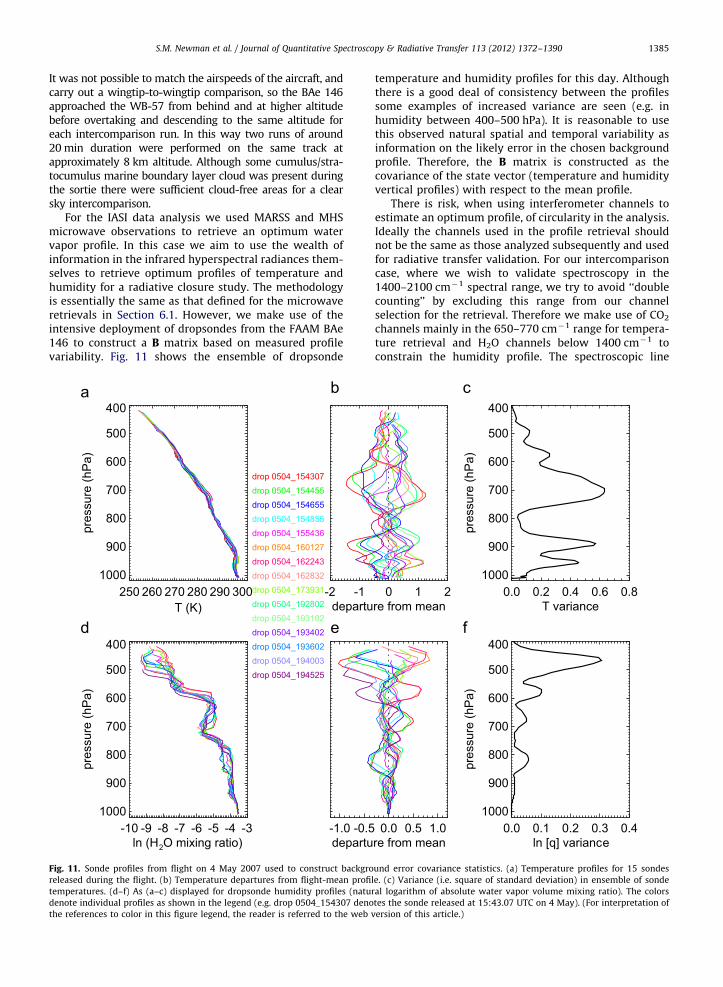
For the IASI data analysis we used MARSS and MHSmicrowave observations to retrieve an optimum watervapor profile. In this case we aim to use the wealth ofinformation in the infrared hyperspectral radiances them-selves to retrieve optimum profiles of temperature andhumidity for a radiative closure study. The methodologyis essentially the same as that defined for the microwaveretrievals in Section 6.1. However, we make use of theintensive deployment of dropsondes from the FAAM BAe146 to construct a B matrix based on measured profilevariability. Fig. 11 shows the ensemble of dropsonde

250 260 270 280 290 300T (K)

1000

900

800

700

600

500

400

pres

sure

(hP

a)

-2 -1departu

drop 0504_154307drop 0504_154455drop 0504_154655drop 0504_154855drop 0504_155436drop 0504_160127drop 0504_162243drop 0504_162832drop 0504_173931drop 0504_192802drop 0504_193102drop 0504_193402drop 0504_193602drop 0504_194003drop 0504_194525

-10 -9 -8 -7 -6 -5 -4 -3ln (H2O mixing ratio)

1000

900

800

700

600

500

400

pres

sure

(hP

a)

-1.0 -0.5departu

Fig. 11. Sonde profiles from flight on 4 May 2007 used to construct backgro

released during the flight. (b) Temperature departures from flight-mean profi

temperatures. (d–f) As (a–c) displayed for dropsonde humidity profiles (natu

denote individual profiles as shown in the legend (e.g. drop 0504_154307 deno

the references to color in this figure legend, the reader is referred to the web v

temperature and humidity profiles for this day. Althoughthere is a good deal of consistency between the profilessome examples of increased variance are seen (e.g. inhumidity between 400–500 hPa). It is reasonable to usethis observed natural spatial and temporal variability asinformation on the likely error in the chosen backgroundprofile. Therefore, the B matrix is constructed as thecovariance of the state vector (temperature and humidityvertical profiles) with respect to the mean profile.

There is risk, when using interferometer channels toestimate an optimum profile, of circularity in the analysis.Ideally the channels used in the profile retrieval shouldnot be the same as those analyzed subsequently and usedfor radiative transfer validation. For our intercomparisoncase, where we wish to validate spectroscopy in the1400–2100 cm�1 spectral range, we try to avoid ‘‘doublecounting’’ by excluding this range from our channelselection for the retrieval. Therefore we make use of CO2

channels mainly in the 650–770 cm�1 range for tempera-ture retrieval and H2O channels below 1400 cm�1 toconstrain the humidity profile. The spectroscopic line

0 1 2re from mean

0.0 0.2 0.4 0.6 0.8T variance

1000

900

800

700

600

500

400

pres

sure

(hP

a)

0.0 0.5 1.0re from mean

0.0 0.1 0.2 0.3 0.4ln [q] variance

1000

900

800

700

600

500

400

pres

sure

(hP

a)

und error covariance statistics. (a) Temperature profiles for 15 sondes

le. (c) Variance (i.e. square of standard deviation) in ensemble of sonde

ral logarithm of absolute water vapor volume mixing ratio). The colors

tes the sonde released at 15:43.07 UTC on 4 May). (For interpretation of

ersion of this article.)

S.M. Newman et al. / Journal of Quantitative Spectroscopy & Radiative Transfer 113 (2012) 1372–13901386

parameters for water in the 800–1200 cm�1 range havebeen shown to have improved significantly in recenteditions of HITRAN [52]. Importantly, we need the Jaco-bians for these water vapor channels to peak at a range ofaltitudes giving sufficient vertical resolution for humidityretrieval, and it was found necessary to include somehigh-peaking channels in the profile retrievals. From Fig. 9it is apparent that the spectral region 1680–1720 cm�1 isrelatively unaffected by changes in water spectroscopyand/or continuum, and channels in this range were alsoused in the retrievals. Channels with significant opticaldepth due to trace gases such as O3 and CH4 wereexcluded.

It is important to ensure that the instrument line shape(ILS) is well represented when computing forward mod-eled radiances and Jacobians. To avoid any artefacts dueto misrepresenting the ILS a Kaiser window function hasbeen applied to the measured radiances for ARIES, S-HISand NAST-I which serves as an apodization function todamp the very highest frequency instrument response(see Section 4.2) without significant loss of spectral

250 260 270 280 290 300Temperature profile (K)

1000

800

600

400

Pre

ssur

e (h

Pa)

Pre

ssur

e (h

Pa)

-9 -8 -7 -6 -5 -4 -3Water vapour profile (ln[VMR])

1000

800

600

400

Pre

ssur

e (h

Pa)

BackgroundARIES retrievalNAST-I retrievalS-HIS retrieval

Pre

ssur

e (h

Pa)

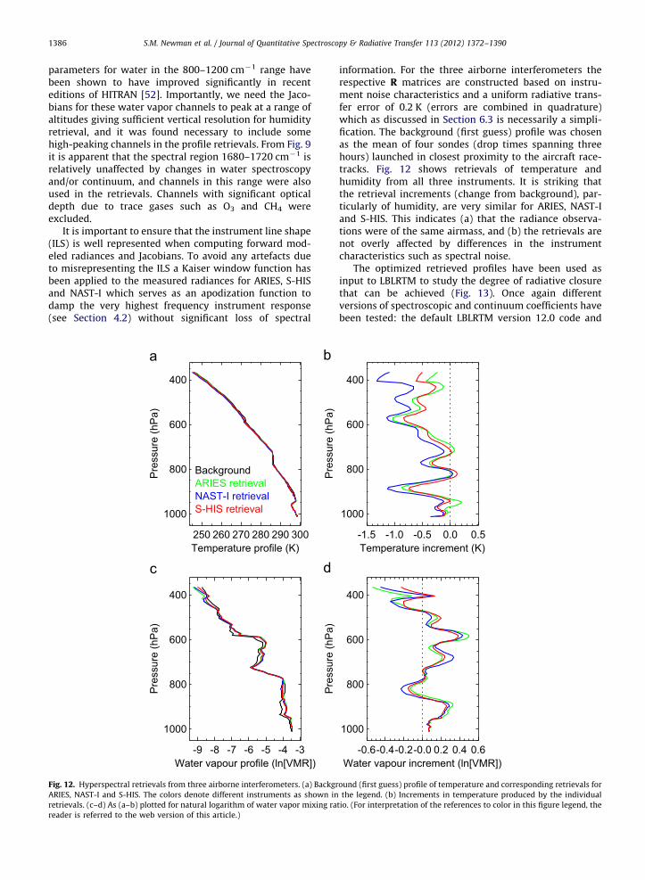
Fig. 12. Hyperspectral retrievals from three airborne interferometers. (a) Backgr

ARIES, NAST-I and S-HIS. The colors denote different instruments as shown in

retrievals. (c–d) As (a–b) plotted for natural logarithm of water vapor mixing ra

reader is referred to the web version of this article.)

information. For the three airborne interferometers therespective R matrices are constructed based on instru-ment noise characteristics and a uniform radiative trans-fer error of 0.2 K (errors are combined in quadrature)which as discussed in Section 6.3 is necessarily a simpli-fication. The background (first guess) profile was chosenas the mean of four sondes (drop times spanning threehours) launched in closest proximity to the aircraft race-tracks. Fig. 12 shows retrievals of temperature andhumidity from all three instruments. It is striking thatthe retrieval increments (change from background), par-ticularly of humidity, are very similar for ARIES, NAST-Iand S-HIS. This indicates (a) that the radiance observa-tions were of the same airmass, and (b) the retrievals arenot overly affected by differences in the instrumentcharacteristics such as spectral noise.

The optimized retrieved profiles have been used asinput to LBLRTM to study the degree of radiative closurethat can be achieved (Fig. 13). Once again differentversions of spectroscopic and continuum coefficients havebeen tested: the default LBLRTM version 12.0 code and

-1.5 -1.0 -0.5 0.0 0.5Temperature increment (K)

1000

800

600

400

-0.6-0.4-0.2-0.0 0.2 0.4 0.6Water vapour increment (ln[VMR])

1000

800

600

400

ound (first guess) profile of temperature and corresponding retrievals for

the legend. (b) Increments in temperature produced by the individual

tio. (For interpretation of the references to color in this figure legend, the

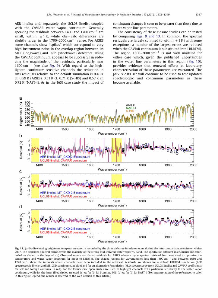
S.M. Newman et al. / Journal of Quantitative Spectroscopy & Radiative Transfer 113 (2012) 1372–1390 1387

AER linelist and, separately, the UCL08 linelist coupledwith the CAVIAR water vapor continuum. Generallyspeaking the residuals between 1400 and 1700 cm�1 aresmall, within 71 K, while obs�calc differences areslightly larger in the 1700–2000 cm�1 range. For ARIESsome channels show ‘‘spikes’’ which correspond to veryhigh instrument noise in the overlap region between itsMCT (longwave) and InSb (shortwave) detectors. Usingthe CAVIAR continuum appears to be successful in redu-cing the magnitude of the residuals, particularly near1600 cm�1 (see also Fig. 9). With regard to the high-lighted continuum-sensitive channels the reduction inrms residuals relative to the default simulation is 0.48 Kcf. 0.59 K (ARIES), 0.51 K cf. 0.71 K (S-HIS) and 0.57 K cf.0.72 K (NAST-I). As in the IASI case study the impact of

1400 1500 1600Wavenum

240250260270280290300

Brig

htne

ss T

(K)

1400 1500 1600Wavenum

-2-1012

Res

idua

l (K

)

1400 1500 1600Wavenum

-2-1012

Res

idua

l (K

)

1400 1500 1600Wavenum

-2-1012

Res

idua

l (K

)

AER linelist, MT_CKD-2.5 continuum

AER linelist, MT_CKD-2.5 continuum

AER linelist, MT_CKD-2.5 continuum

UCL08 linelist, CAVIAR continuum

UCL08 linelist, CAVIAR continuum

UCL08 linelist, CAVIAR continuum

Fig. 13. (a) Nadir-viewing brightness temperature spectra recorded by the thre

2007. The displayed spectral range covers the majority of the strong mid-infrar

coded as shown in the legend. (b) Observed minus calculated residuals for

temperature and water vapor spectrum for input to LBLRTM. The shaded re

1720 cm�1 show the intervals where channels have been included in the

spectroscopic linelist and MT_CKD continuum, in blue) and for an alternative for

for self and foreign continua, in red). For the former case open circles are us

continuum, while for the latter filled circles are used. (c) As for (b) for Scanning-

in this figure legend, the reader is referred to the web version of this article.)

continuum changes is seen to be greater than those due towater vapor line parameters.

The consistency of these closure studies can be testedby comparing Figs. 9 and 13. In common, the spectralresiduals are largely confined to within 71 K (with someexceptions: a number of the largest errors are reducedwhen the CAVIAR continuum is substituted into LBLRTM).The region 1800–2000 cm�1 is not well modeled foreither case which, given the published uncertaintiesin the water line parameters in this region (Fig. 10),provides evidence that renewed efforts at laboratorycharacterization of these parameters are warranted. TheJAIVEx data set will continue to be used to test updatedspectroscopic and continuum parameters as thesebecome available.

1700 1800 1900 2000ber (cm-1)

ARIESNAST-IS-HIS

1700 1800 1900 2000ber (cm-1)

1700 1800 1900 2000ber (cm-1)

1700 1800 1900 2000ber (cm-1)

e airborne interferometers during the intercomparison exercise on 4 May

ed water vapor n2 band. The spectra for different instruments are color-

ARIES where a hyperspectral retrieval has been used to optimize the

gions for wavenumbers less than 1400 cm�1 and between 1680 and

retrieval. Residuals are shown for a default LBLRTM simulation (AER

mulation (H2O spectroscopy from UCL08 linelist and CAVIAR coefficients

ed to highlight channels with particular sensitivity to the water vapor

HIS. (d) As for (b) for NAST-I. (For interpretation of the references to color

S.M. Newman et al. / Journal of Quantitative Spectroscopy & Radiative Transfer 113 (2012) 1372–13901388

7. Discussion and conclusions

JAIVEx was conceived as an experiment to test theabsolute radiometric accuracy of the IASI instrument andto validate the fundamental radiative transfer that under-pins its applications in NWP and climate science. Themission’s goal of retrieving temperature structures towithin 71 K and humidity to within 710%, at 1 kmvertical resolution, relies on the ability to model IASIradiances with high accuracy (or, the avoidance of channelswith large forward model uncertainty [51]). Through directcomparison of spatially and temporally co-located interfe-rometers on MetOp, the NASA WB-57 and FAAM BAe 146,we find that only 0.3 K separates the independent bright-ness temperature measurements in transparent atmo-spheric micro-windows. This figure, which comparesfavorably with the design specification of 0.5 K [15], iscorroborated by results from other studies. For example,Larar et al. [6] found that spectra from WB-57 NAST-Iobservations and IASI radiances were within �0.1 K(band-averaged); using NAST-I as a calibration referencestandard for computing double-differences, they demon-strated longwave band differences between IASI and AIRS ofless than 0.05 K. Blumstein et al. [53] report the differencebetween IASI and AIRS to be less than 0.1 K when analyzingchannels in the 600–1500 cm�1 spectral range. Wang et al.[54] found AIRS to be slightly warmer than IASI by less than0.1 K. Aumann and Pagano [55], in another AIRS-IASI cross-comparison, found a statistically insignificant drift ofapproximately 0.02 K over six months. Taken together, theseresults confirm the impressive stability and absolute radio-metric accuracy of IASI to date.

In the context of radiative closure, discrepanciesbetween measured and modeled radiances must be parti-tioned between instrument calibration error and/or noise,uncertainty in the atmospheric profile and/or surfacecharacteristics, or radiative transfer model error. Theconfirmation of IASI, NAST-I, S-HIS and ARIES mutualcalibration accuracy means we can have confidence thatspectral residuals will not be dominated by instrumenterror artifacts. For the IASI CO2 sounding channels in the650–770 cm�1 spectral range, making use of in situ truthCO2 concentrations, we find that GENLN2 simulations areunable to reproduce IASI brightness temperatures to thesame accuracy as kCARTA and LBLRTM models. This isperhaps not surprising since the latter codes employ morerecently developed line shape models. It does emphasizethe need for radiative transfer codes to be updatedregularly with the latest spectroscopic parameters.

As a means of minimizing profile error we employmicrowave and hyperspectral infrared retrievals of theatmospheric state, primarily to reduce the uncertaintyin the water vapor profile. We find that IASI–LBLRTMresiduals in the 1400–2070 cm�1 range are modestlyimproved through the use of the UCL08 water vaporlinelist which includes many weaker lines not found inHITRAN 2008. Even more significantly, we find that recentlaboratory measurements of the water vapor continuumare a better fit to the IASI spectra than MT_CKD-2.5.

Analysis of ARIES, S-HIS and NAST-I radiances from theJAIVEx intercomparison flight reinforce the finding that

the CAVIAR (RAL MSF) continuum is a good fit to thespectra in these specific campaign conditions. We notethat the JAIVEx case studies were conducted over the Gulfof Mexico in a warm, moist atmosphere. Hence, we mightexpect laboratory continuum coefficients derived at roomtemperature to be a better match than cases in colder,drier atmospheres. In a study of mid-latitude FAAM flightsNewman et al. [56] found limited agreement betweenobserved and modeled radiances using the CAVIARlaboratory-derived continuum coefficients in the 1300–2000 cm�1 range. Discrepancies were seen between con-tinuum strengths derived for observations sensitive todifferent effective temperatures, which suggests theremay be a weak foreign continuum temperature depen-dence. In a set of measurements from Antarctica around�30 1C Rowe and Walden [57] retrieved continuumcoefficients at variance with MT_CKD, while laboratorymeasurements in the range 296–351 K [58] also show atentative trend of foreign continuum strength with tem-perature. Future work will need to focus on whether thispostulated temperature dependence is genuine given thepotential impact on modeled brightness temperatures forspaceborne instruments.

Acknowledgments

We thank Nigel Atkinson and Peter Schlussel for timelyprovision of IASI data during the JAIVEx campaign, andAndrew Collard and Fiona Hilton for archiving modelfields. We also thank Sergio de Souza-Machado for sup-plying the kCARTA software and Jonathan Tennyson formaking the UCL08 linelist available. The contributions ofmany people involved in JAIVEx are gratefully acknowl-edged. This work was partially funded under EUMETSATContract Eum/CO/06/1596/PS. Airborne data were obtainedusing the BAe-146-301 Atmospheric Research Aircraft (ARA)flown by Directflight Ltd. and managed by the Facility forAirborne Atmospheric Measurements (FAAM), which is ajoint entity of the Natural Environment Research Council(NERC) and the Met Office. The authors acknowledge theNERC-funded Rutherford Appleton Laboratory MolecularSpectroscopy Facility for their contribution to the derivationof the CAVIAR continuum coefficients.

References

[1] Smith WL, Revercomb H, Bingham G, Larar A, Huang H, Zhou D,et al. Technical note: evolution, current capabilities, and futureadvance in satellite nadir viewing ultra-spectral IR sounding of thelower atmosphere. Atmos Chem Phys 2009;9:5563–74.

[2] Prunet P, Thepaut JN, Casse V. The information content of clear skyIASI radiances and their potential for numerical weather prediction.Q J R Meteorol Soc 1998;124:211–41.

[3] Hilton F, Atkinson NC, English SJ, Eyre JR. Assimilation of IASI at theMet Office and assessment of its impact through observing systemexperiments. Q J R Meteorol Soc 2009;135:495–505.

[4] Zhou DK, Smith WL, Larar AM, Liu X, Taylor JP, Schlussel P, et al. Allweather IASI single field-of-view retrievals: case study—validationwith JAIVEx data. Atmos Chem Phys 2009;9:2241–55.

[5] Thelen JC, Havemann S, Newman SM, Taylor JP. Hyperspectralretrieval of land surface emissivities using ARIES. Q J R MeteorolSoc 2009;135:2110–24.

[6] Larar AM, Smith WL, Zhou DK, Liu X, Revercomb H, Taylor JP, et al.IASI spectral radiance validation inter-comparisons: case study

S.M. Newman et al. / Journal of Quantitative Spectroscopy & Radiative Transfer 113 (2012) 1372–1390 1389

assessment from the JAIVEx field campaign. Atmos Chem Phys2010;10:411–30.

[7] Grieco G, Masiello G, Serio C, Jones RL, Mead MI. Infrared atmo-spheric sounding interferometer correlation interferometry for theretrieval of atmospheric gases: the case of H2O and CO2. Appl Opt2011;50:4516–28.

[8] Coudert LH, Wagner G, Birk M, Baranov YI, Lafferty WJ, Flaud JM.The (H2O)–O-16 molecule: line position and line intensity analysesup to the second triad. J Mol Spectrosc 2008;251:339–57.

[9] Flaud J-M, Piccolo C, Carli B, Perrin A, Coudert LH, Teffo J-L, et al.Molecular line parameters for the MIPAS (Michelson Interferometerfor Passive Atmospheric Sounding) experiment. Atmos Oceanic Opt2003;16:172–81.

[10] Te Y, Payan S, Jeseck P, Bureau J, Camy-Peyret C. Recent resultsobtained with the IASI-balloon experiment and contribution to thecalibration/validation of IASI on MetOp. In: Conroy L, editor.Proceedings of the 18th ESA symposium on European rocket andballoon programmes and related research, vol. 647. ESA SpecialPublications; 2007. p. 147–53.

[11] Razavi A, Clerbaux C, Wespes C, Clarisse L, Hurtmans D, Payan S,et al. Characterization of methane retrievals from the IASI space-borne sounder. Atmos Chem Phys 2009;9:7889–99.

[12] Rothman LS, Gordon IE, Barbe A, Benner DC, Bernath PE, Birk M,et al. The HITRAN 2008 molecular spectroscopic database. J QuantSpectrosc Radiat Transfer 2009;110:533–72.

[13] Jacquinet-Husson N, Scott NA, Chedina A, Crepeau L, Armante R,Capelle V, et al. The GEISA spectroscopic database: current andfuture archive for Earth and planetary atmosphere studies. J QuantSpectrosc Radiat Transfer 2008;109:1043–59.

[14] Chahine MT, Pagano TS, Aumann HH, Atlas R, Barnet C, Blaisdell J,et al. AIRS: Improving weather forecasting and providing new dataon greenhouse gases. Bull Am Meteorol Soc 2006;87:911–26.

[15] Simeoni D, Singer C, Chalon G. Infrared atmospheric soundinginterferometer. Acta Astronaut 1997;40:113–8.

[16] Tobin DC, Revercomb HE, Knuteson RO, Best FA, Smith WL,Ciganovich NN, et al. Radiometric and spectral validation of atmo-spheric infrared sounder observations with the aircraft-based scan-ning high-resolution interferometer sounder. J Geophys Res—Atmos2006;111:D09S02.

[17] Smith WL, Zhou DK, Larar AM, Mango SA, Howell HB, Knuteson RO,et al. The NPOESS airborne sounding testbed interferometer—remotelysensed surface and atmospheric conditions during CLAMS. J Atmos Sci2005;62:1118–34.

[18] Wilson SHS, Atkinson NC, Smith JA. The development of an airborneinfrared interferometer for meteorological sounding studies.J Atmos Oceanic Technol 1999;16:1912–27.

[19] Vaisala technical document. GPS Dropwindsonde RD93 and AircraftData System AVAPS. Ref. A606en 1998-05.

[20] Shephard MW, Clough SA, Payne VH, Smith WL, Kireev S,Cady-Pereira KE. Performance of the line-by-line radiative transfermodel (LBLRTM) for temperature and species retrievals: IASI casestudies from JAIVEx. Atmos Chem Phys 2009;9:7397–417.

[21] Clough SA, Shephard MW, Mlawer E, Delamere JS, Iacono M,Cady-Pereira K, et al. Atmospheric radiative transfer modeling: asummary of the AER codes. J Quant Spectrosc Radiat Transfer 2005;91:233–44.

[22] Newman SM, Smith JA, Glew MD, Rogers SM, Taylor JP. Tempera-ture and salinity dependence of sea surface emissivity in thethermal infrared. Q J R Meteorol Soc 2005;131:2539–57.

[23] Kaiser JF, Schafer RW. On the use of the Io-Sinh Window forspectrum analysis. IEEE Trans Acoust Speech Signal Process1980;ASSP-28(1):105–7, doi:10.1109/TASSP.1980.1163349.

[24] Armstrong BH. Spectrum line profiles: the Voigt function. J QuantSpectrosc Radiat Transfer 1967;7:66–88.

[25] Edwards DP, Strow LL. Spectral-line shape considerations for limbtemperature sounders. J Geophys Res—Atmos 1991;96:20859–68.

[26] Cousin C, Ledoucen R, Boulet C, Henry A. Temperature-dependenceof the absorption in the region beyond the 4.3 mm band head ofCO2. 2: N2 and O2 broadening. Appl Opt 1985;24:3899–907.

[27] Strow LL, Hannon SE, De Souza-Machado S, Motteler HE, Tobin D.An overview of the AIRS radiative transfer model. IEEE Trans GeosciRemote Sensing 2003;41:303–13.

[28] Lamouroux J, Tran H, Laraia AL, Gamache RR, Rothman LS, GordonIE, et al. Updated database plus software for line-mixing inCO(2) infrared spectra and their test using laboratory spectra inthe 1.5–2.3 mm region. J Quant Spectrosc Radiat Transfer 2010;111:2321–31.

[29] Niro F, Jucks K, Hartmann JM. Spectra calculations in central andwing regions of CO2IR bands. IV: software and database for the

computation of atmospheric spectra. J Quant Spectrosc RadiatTransfer 2005;95:469–81.

[30] Mlawer EJ, Payne VH, Moncet J-L, Delamere JS, Alvarado MJ, TobinDD. Development and recent evaluation of the MT_CKD model ofcontinuum absorption. Philos Trans R Soc A, doi:10.1098/rsta.2011.0295, in press.

[31] Newman SM, Knuteson RO, Zhou DK, Larar AM, Smith WL, TaylorJP. Radiative transfer validation study from the European AquaThermodynamic Experiment. Q J R Meteorol Soc 2009;135:277–90.

[32] Hilton FI, Newman SM, Collard AD. Identification of NWP humiditybiases using high-peaking water vapour channels from IASI. AtmosSci Lett 2012;13:73–8.

[33] Turner DD, Tobin DC, Clough SA, Brown PD, Ellingson RG, MlawerEJ, et al. The QME AERI LBLRTM: a closure experiment for down-welling high spectral resolution infrared radiance. J Atmos Sci2004;61:2657–75.

[34] McGrath A, Hewison T. Measuring the accuracy of MARSS—anairborne microwave radiometer. J Atmos Oceanic Technol 2001;18:2003–12.

[35] Bonsignori R. The microwave humidity sounder (MHS) in-orbitperformance assessment. Int Soc Opt Eng (SPIE Proc) 2007;6744:67440A, doi:10.1117/12.737986.

[36] Haefele A, Kampfer N. Tropospheric water vapor profiles retrievedfrom pressure-broadened emission spectra at 22 GHz. J AtmosOceanic Technol 2010;27:167–72.

[37] Rabier F, Fourrie N, Chafai D, Prunet P. Channel selection methodsfor infrared atmospheric sounding interferometer radiances. Q J RMeteorol Soc 2002;128:1011–27.

[38] Liu X, Zhou DK, Larar AM, Smith WL, Schluessel P, Newman SM, et al.Retrieval of atmospheric profiles and cloud properties from IASIspectra using super-channels. Atmos Chem Phys 2009;9:9121–42.

[39] Rodgers CD. Inverse methods for atmospheric sounding: theory andpractice. Series on atmospheric, oceanic and planetary physics—

vol. 2. World Scientific; 2000.[40] Hewison TJ. Aircraft validation of clear air absorption models at

millimeter wavelengths (89–183 GHz). J Geophys Res—Atmos2006;111:D14303.

[41] Kleespies TJ, Watts P. Comparison of simulated radiances, Jacobiansand linear error analysis for the Microwave Humidity Sounder andthe Advanced Microwave Sounding Unit-B. Q J R Meteorol Soc2006;132:3001–10.

[42] Turner DD, Cadeddu MP, Lohnert U, Crewell S, Vogelmann AM.Modifications to the water vapor continuum in the microwavesuggested by ground-based 150-GHz observations. IEEE TransGeosci Remote Sensing 2009;47:3326–37.

[43] AJL Shillings, Ball SM, Barber MJ, Tennyson J, Jones RL. An upperlimit for water dimer absorption in the 750 nm spectral region anda revised water line list. Atmos Chem Phys 2011;11:4273–87.

[44] Ptashnik IV, McPheat RA, Shine KP, Smith KM, Williams RG. Watervapor self-continuum absorption in near-infrared windows derivedfrom laboratory measurements. J Geophys Res—Atmos 2011;116:D16305.

[45] Ptashnik IV, McPheat RA, Shine KP, Smith KM, Williams RG. Watervapor foreign continuum absorption in near-infrared windowsfrom laboratory measurements. Philos Trans R Soc A, doi:10.1098/rsta.2011.0218, in press.

[46] Brown LR, Benner DC, Devi VM, Smith MAH, Toth RA. Line mixing inself- and foreign-broadened water vapor at 6 mm. J Mol Struct2005;742:111–22.

[47] Boone CD, Walker KA, Bernath PF. An efficient analytical approachfor calculating line mixing in atmospheric remote sensing applica-tions. J Quant Spectrosc Radiat Transfer 2011;112:980–9.

[48] Tran H, Flaud PM, Gabard T, Hase F, von Clarmann T, Camy-Peyret C,et al. Model, software and database for line-mixing effects in thenu(3) and nu(4) bands of CH4 and tests using laboratory and planetarymeasurements—I: N2 (and air) broadenings and the earth atmo-sphere. J Quant Spectrosc Radiat Transfer 2006;101:284–305.

[49] Rothman LS, Jacquemart D, Barbe A, Benner DC, Birk M, Brown LR,et al. The HITRAN 2004 molecular spectroscopic database. J QuantSpectrosc Radiat Transfer 2005;96:139–204.

[50] McClatchey RA, Fenn RW, Selby JEA, Volz FE, Garing JS. Opticalproperties of the atmosphere. 3rd editionBedford, Massachusetts:Air Force Cambridge Research Lab; 1972 [Environmental researchpapers no. 411].

[51] Collard AD. Selection of IASI channels for use in numerical weatherprediction. Q J R Meteorol Soc 2007;133:1977–91.

[52] Newman SM, Taylor JP. Impact of updates to the HITRAN spectro-scopic database on the modeling of clear-sky infrared radiances.Geophys Res Lett 2002;29:1957.

S.M. Newman et al. / Journal of Quantitative Spectroscopy & Radiative Transfer 113 (2012) 1372–13901390

[53] Blumstein D, Tournier B, Cayla FR, Phulpin T, Fjortoft R, Buil C, et al.In-flight performance of the infrared atmospheric sounding inter-ferometer (IASI) on METOP-A—art. no. 66840H. In: Goldberg MD,Bloom HJ, Huang AH, Ardanuy PE, editors. Atmospheric andenvironmental remote sensing data processing and utilization III:readiness for Geoss. Proceedings of the society of photo-opticalinstrumentation engineers (SPIE), vol. 6684. Bellingham: SPIE—International Society of Optical Engineering; 2007. p. H6840.

[54] Wang LK, Wu XQ, Li YP, Goldberg M, Sohn SH, Cao CY. Comparisonof AIRS and IASI radiances using GOES imagers as transfer radio-meters toward climate data records. J Appl Meteorol Climatol2010;49:478–92.

[55] Aumann HH, Pagano TS. Using AIRS and IASI data to evaluate absoluteradiometric accuracy and stability for climate applications. In: GoldbergMD et al., editors. Atmospheric and environmental remote sensing data

processing and utilization IV: readiness for GEOSS II. InternationalSociety for Optical Engineering (SPIE Proceedings, vol. 7085); 2008.

p. 708504. doi:10.1117/12.795225.[56] Newman SM, Green PD, Ptashnik IV, Gardiner TD, Coleman MD,

McPheat RA, et al. Airborne and satellite remote sensing of the mid-infrared water vapour continuum. Philos Trans R Soc A, doi:10.1098/rsta.2011.0223, in press.

[57] Rowe PM, Walden VP. Improved measurements of the foreign-broadened continuum of water vapor in the 6.3 mm band at �30

degrees C. Appl Opt 2009;48:1358–65.[58] Paynter DJ, Ptashnik IV, Shine KP, Smith KM, McPheat R, Williams

RG. Laboratory measurements of the water vapor continuum in the1200–8000 cm�1 region between 293 K and 351 K. J GeophysRes—Atmos 2009;114:D21301.