The Limited Influence of Unemployment on the Wage Bargain∗

Robert E. HallHoover Institution and Department of Economics

rehall@stanford.edu stanford.edu/∼rehall

Paul R. MilgromDepartment of Economics

milgrom@stanford.edu www.milgrom.net

Stanford University

October 20, 2007

Abstract

When a job-seeker and an employer meet, find a prospective joint surplus, and bargain overthe wage, conditions in the outside labor market, including especially unemployment, mayhave limited influence. The job-seeker’s only credible threat during bargaining is to hold outfor a better deal, not to terminate bargaining and resume search at other employers. Similarly,the employer’s threat is to delay bargaining, not to terminate it. Consequently, the outcomeof the bargain depends on the relative costs of delays to the parties, rather than on the payoffsthat result from exiting negotiations. Modelling bargaining in this way makes wages lessresponsive to unemployment. A stochastic model of the labor market with credible bargainingand reasonable parameter values yields larger employment fluctuations than does the standardMortensen-Pissarides model.

∗We are grateful to Daron Acemoglu, John Kennan, Dan Quint, Randy Wright, four referees, and the editor forcomments. Hall’s research is part of the program on Economic Fluctuations and Growth of the NBER. A file containingthe calculations is available at Stanford.edu/∼rehall

1

1 Introduction

Congratulations! You made it through the interview process. Both you and the hiring

manager agree that you are the right person for the job. Now, however, you must

negotiate the terms of the job offer.

So begins Wegerbauer (2000), a book offering advice to job-seekers about dealing with a prospec-

tive employer. If terms are indeed determined by negotiation after a match has been identified,

then the nature of the negotiation has a role in determining the employer surplus. Anticipation of

that surplus influences the employers’ recruiting efforts, which affects the level of unemployment.

We show that replacing the traditional model of bargaining with a more credible alternating offer

bargaining model leads to weaker feedback from current unemployment levels to the current wage.

Consequently, when the labor market is hit with productivity shocks, the credible bargaining model

delivers greater variation in employer surplus, employer recruiting efforts, and employment than

the ”Nash” bargaining model.

The model of the wage-setting process at the heart of our analysis is a non-cooperative alter-

nating offer model and improves on two common conceptions of wage bargaining. According to

one conception, employers set wages and other terms and hire the most qualified applicant willing

to work on those terms. The terms are offered to applicants on a strict take-it-or-leave-it basis.

We believe that this model fails in an important way to describe much of the labor market, though

essentially no research has studied the question.

A second common conception, which forms the basis of a large literature whose canon is

Mortensen and Pissarides (1994), has wages and other terms of employment set by a “Nash bar-

gain.” Models using this formulation assume that the threat point for bargaining is the payoff pair

that results when the job-seeker returns to the market and the employer waits for another applicant.

A consequence is that the bargained wage is a weighted average of the applicant’s productivity

in the job and the value of unemployment. That latter value, in turn, depends in large part on

the wages offered in other jobs. If an adverse unit productivity shock reduces every employer’s

reservation wage by one unit, then both terms in the average fall by almost equal amounts. If

both changed by exactly one unit, then the employer’s recruiting effort would be unchanged and

unemployment would not fluctuate. The actual equilibrium is similar to this approximate equilib-

rium and cannot explain realistic employment fluctuations. This is the point of an influential paper,

Shimer (2005).

2

This flexible-wage conclusion, however, hinges on unrealistic assumptions about bargaining

threats, which we challenge. Once a qualified worker meets an employer, a threat to walk away,

permanently terminating the bargain, is not credible. The bargainers have a joint surplus, arising

from search friction, that glues them together. We make use of bargaining theory from Binmore,

Rubinstein and Wolinsky (1986) to invoke more realistic threats during bargaining. The threats are

to extend bargaining rather than to terminate it. The result is to loosen the tight connection between

wages and outside conditions of the Mortensen-Pissarides model. In our model, a job-seeker loses

most of the connection with outside conditions the moment she encounters a suitable employer, but

before she makes her wage bargain. The bargain is controlled by the job’s productivity and by her

patience as a bargainer relative to the employer’s. The possibility that she will return to job search

remains in the picture because the job opportunity may disappear during bargaining, but this factor

has a secondary influence.

The model delivers substantial volatility of unemployment through a mechanism similar to the

one in Hall (2005a)—unemployment is high in periods when the wage bargain is unfavorable to

employers. In times of low productivity, the wage falls only partly in response, the burden of the

rest of the decline falls on employers. Because they have less to gain by hiring a worker, employers

put fewer resources into recruiting, and the labor market is slacker.

Wage negotiations between General Motors and the United Auto Workers illustrate the key

change we make to the bargaining model (see Holden (1997) for an application of the BRW theory

in the union setting). The wage agreement depends on the losses the bargainers suffer during a

strike or lock-out. Each side is keenly aware of the costs of delay that fall on themselves and on

the other side. The union accumulates strike funds and the company accumulates inventories to

lower the costs of holding out for a better deal. The union never seriously considers permanent

resignation of the workers as an option and GM does not consider discharging the workers per-

manently. Except in extreme circumstances, neither threat would be credible, because the workers

would do better to accept a reduced wage than to quit, and GM would do better to pay a higher

wage than to start over with new workers. This observation has important consequences for the

comparative statics of the bargaining model. For example, if a new law were to make it costlier for

GM to discharge its workforce during a work stoppage, that would be predicted to have no effect

on the wage bargain.

Similarly, the non-cooperative bargaining model of Binmore et al. (1986) distinguishes be-

tween theoutside-optionpayoff that the parties get by quitting the negotiation to seek other oppor-

3

tunities and thedisagreement payoffthat the parties get during the bargaining, during the disagree-

ment period before the agreement is reached. Unless the outside option is especially favorable, it

is the disagreement payoff—not the outside option—that determines the bargaining outcome.

In the alternating offer wage-bargaining environment, so long as reaching an agreement creates

value, a bargainer who gets a poor offer continues to bargain, because that choice has a strictly

higher payoff than taking the outside option. Threats to exercise the outside option simply are

not credible. Since this is common knowledge, changes in the value of the outside option cannot

affect the bargaining outcome. In the BRW equilibrium, the parties do not actually spend any

time bargaining. They think through the consequences of a sequence of offers and counteroffers

and then move immediately to an agreement at the unique subgame perfect equilibrium of the

bargaining game. They do not waste time and resources haggling over the wage.

In the MP class of models, conclusions about the insensitivity of compensation to unemployment—

and the resulting high sensitivity of unemployment to driving forces—depend on certain key para-

meters. One is the elasticity of labor supply. Hagedorn and Manovskii (2006) demonstrate that the

standard MP model delivers high sensitivity of unemployment to driving forces when labor supply

is highly elastic. In that case, workers are close to indifferent to working or searching (in a sense

we explain later), so small changes in the incentive to work cause large changes in the volume of

search. We review the evidence on labor supply and find that the elasticity needed to generate the

observed volatility of unemployment is far higher than the findings from research on labor sup-

ply. Our bargaining model delivers a realistic unemployment response to productivity shifts with

a labor-supply elasticity in line with that research

For our model, a second key parameter is the cost of recruitment. We take this cost from data

on hiring cost reported by employers. If we use a higher figure, the sensitivity of unemployment to

productivity is lower. The success of our explanation of unemployment volatility depends on the

realism of our inputs.

We model shifts in labor demand as changes in productivity, defined as the ratio of output to la-

bor input. This incorporates shifts in labor demand arising from changes in total factor productivity

and in the prices of other inputs.

Although this paper is about the limited response of the wage to conditions in the labor market,

we do not provide direct evidence on the flexibility or stickiness of wages. We are skeptical about

recent attempts to measure wage flexibility. Our strategy is to measure the empirical relation

between productivity fluctuations and unemployment, to confirm that the MP model with standard

4

parameter values falls far short of replicating the observed volatility of unemployment induced by

productivity fluctuations, and to compare two models that are successful, the one in Hagedorn and

Manovskii’s (2006) paper and the one developed here. Following Mortensen andEva Nagypal

(2007), our perspective differs substantially from Shimer’s (2005), who considers not the part of

unemployment volatility induced by productivity variation, but rather all of the volatility. We show

that productivity can account for only a fraction of unemployment volatility, and use that amount

as our benchmark of explanatory success.

2 Model

Mortensen and Pissarides (1994) introduced a model that provides the foundation for a large

amount of recent research on labor-market fluctuations. Part of that research, including this pa-

per, retains all the elements of the MP model except its Nash bargain for wages. We refer to the

MP class of models as those like ours that change only the wage determination specification. Our

discussion begins with the elements we take over without change from the MP model.

2.1 Elements common to the MP class of models

The driving force of the model is productivity,pi, wherei is a discrete stationary state variable

i ∈ [1, . . . , N ] with transition matrixπi,i′. Workers and employers are risk-neutral. Their discount

rate is equal to the interest rate,r.

We start by describing the mechanism by which employers and workers match. Matching

results from non-contractible pre-match effort by employers—help-wanted advertising and other

recruiting costs—reinforced by the search time of job-seekers. It is conventional to describe the

mechanism in terms of vacancies, though this concept need be nothing more than a metaphor

capturing recruiting effort of many kinds. The key variable isθi, the ratio of vacancies to un-

employment. The job-finding rate depends onθi according to the increasing functionφ(θi) and

the recruiting rate is the decreasing functionφ(θi)θi

. The separation rate—the per-period probability

that a job will end—is an exogenous constants (see Hall (2005b) for evidence supporting this

proposition).

During a period, an individual may be seeking a job or working and an employer may have a

number of vacancies open and a number of employees. At the end of the period, the job seeker

finds a potential position with probabilityφ(θi). The job-seeker and the employer bargain for a

wage with present valueWi for the job to start at the beginning of the next period. Our model

5

implies that bargaining always results in employment, soφ(θi) is also the job-finding rate. A

vacancy is filled with a new hire with probabilityφ(θi)θi

. An employee departs the firm at the end

of the period with probabilitys. Finally, at the beginning of the next period, the firm decides how

many vacancies to hold open during the period.

Three values characterize the job-seeker’s bargaining position. If unemployed, the job-seeker

achieves a valueUi. Upon finding a job, she receives a wage contract with a present value ofWi and

also enjoys a valueVi for the rest of her career, starting with the period of job search that follows

the job. While searching, a job-seeker receives a flow valuez per period. She has a probability

φ(θi), the job-finding rate, of finding and starting a new job. HenceUi must satisfy

Ui = z +1

1 + r

∑i′πi,i′ [φ(θi′)(Wi′ + Vi′) + (1− φ(θi′))Ui′ ] . (1)

Similarly,Vi must satisfy

Vi =1

1 + r

∑i′πi,i′ [sUi′ + (1− s)Vi′ ] . (2)

The value of the outside option of the job-seeker when bargaining over the wage with a prospective

employer isUi.

Workers produce output with a flow value ofpi, the marginal product of labor. The present

value,Pi, of the output produced over the course of a job is:

Pi = pi +1

1 + r

∑i′πi,i′(1− s)Pi′ . (3)

The model assumes free entry on the employer side, so that the expected profit from initiating

the recruitment of a new worker by opening a vacancy is zero. In that case, employer pre-match

cost equals the employer’s expected share of the match surplus. Employers control the resources

that govern the job-finding rate. The incentive to deploy the resources is the employer’s net value

from a match,Pi −Wi. Recruiting to fill a vacancy costsc per period, payable at the end of the

period. The zero-profit condition is:

φ(θi)

θi(Pi −Wi) = c. (4)

Employers create vacancies, drive up the vacancy/unemployment ratioθi, and drive down the re-

cruiting rate to the point that satisfies the zero-profit condition. Because of free entry, the em-

ployer’s outside option while bargaining with a worker has value zero. Notice that we require that

6

the zero-profit condition hold for each value of the driving forcei; this is what makes recruiting

effort vary withi.

Equation (4) has an implication of central importance in the rest of the paper. Given a wage

Wi, the zero-profit condition determinesθi and thus unemployment. If the wage is flexible in the

sense that employer surplusPi −Wi is nearly independent of the state, then unemployment has

low volatility. In contrast, if the wage is sticky, so that the gap between productivity and the wage

rises quickly with productivity, then unemployment will fall sharply when productivity rises, so

the volatility of unemployment will be much higher. In the class of models considered here, which

differ only in their wage-determination specifications,wage stickiness is the sole determinant of

unemployment volatility. We need not investigate wage stickiness and unemployment volatility

separately. We stress that this conclusion applies only in the class of models we are considering.

Pissarides (2007) describes models with elements such as on-the-job search where stickiness and

unemployment volatility are not locked together.

2.2 The wage bargain in the original MP model

In the set-up just described, the worker and employer have a prospective joint surplus ofPi+Vi−Ui,the difference between the value created by this job and the worker’s subsequent career,Pi + Vi,

and the worker’s non-match value,Ui. The original MP model posits that the worker and employer

receive given fractionsβ and1 − β of that surplus. The job-seeker’s threat point is the value

achieved during the prospective employment period by disclaiming the current job opportunity

and continuing to search, that is, the unemployment value,Ui. The worker’s value,Wi + Vi, is this

threat value plus the fractionβ of the surplus:

Wi + Vi = Ui + β(Pi + Vi − Ui), (5)

so the worker’s wage is:

Wi = βPi + (1− β)(Ui − Vi). (6)

The developers of this model often rationalized this wage rule as a Nash bargain.

The model has5N endogenous variables, the worker’s value of being unemployed,Ui, her

value of employment after the prospective job,Vi, the vacancy/unemployment ratio,θi, the present

value of productivity,Pi, and the present value of wage payments,Wi. It has5N equations, (1),

(2), (3), (4), and (6).

7

From the solution, we can calculate other variables, including the unemployment rate,u. In

stochastic equilibrium while in statei, the flow rate of workers into unemployment iss(1 − ui)

equals the flow rate out of unemployment,φ(θi)ui. Although in principleu is a separate state

variable, it moves so much faster thani that we can use the stochastic equilibrium value as a close

approximation to the actual value of unemployment:

ui =s

s+ φ(θi). (7)

In this model, the wage is the weighted average of productivityPi and the worker’s opportunity

cost,Ui−Vi. In the usual calibration withβ around 0.5, the wage is highly responsive to changes in

productivity becausePi andUi−Vi move together—the worker’s opportunity costUi−Vi depends

sensitively on the wages of other jobs. Indeed, in the calibration we attribute to Mortensen and

Pissarides,Wi changes by 93 percent of the change inPi. Thus, a transition from one level ofPi to

a lower one results in correspondingly large changes inWi but only tiny changes in unemployment.

This flexible-wage property of the standard model is the point of Shimer (2005).

2.3 The alternating-offer wage bargain

In our bargaining model, adapted from Binmore et al. (1986), bargaining takes place over time.

The parties alternate in making proposals. After a proposer makes an offer, the responding party

has three options: accept the current proposal, reject it and make a counter-proposal, or abandon

the bargaining and take the outside option. The abandonment of bargaining by either party results

in lump-sum payoffs of zero for the employer andUi for the worker. If the responding party

makes a counter-proposal, both parties receive the disagreement payoff for that period and the

game continues. The employer incurs a costγ > 0 each time it formulates a counteroffer to the

worker. The worker receives the flow benefitz while bargaining. Notice that our sign convention

is the opposite for workers and employers—workers have a benefitz from waiting and firms incur

a costγ.

In this bargaining game, when the joint payoff from matching,Vi+Pi, exceeds both the unem-

ployment payoffUi and the capitalized flow1+rr

(z − γ), the parties agree on a wageWi < Pi. If

Vi + Pi falls short of either of the other two values, no agreement is reached. IfVi + Pi = Ui, the

wage could bePi but then employment will not occur because there is no incentive for recruiting

effort by employers. The same is true ifVi +Pi = 1+rr

(z− γ). Our exposition emphasizes the first

possibility for every statei, because it is the only one that can justify positive search by employers

and positive equilibrium employment in every state.

8

We temporarily assume that the subgame perfect equilibrium of the bargaining models begin-

ning with a proposal by the employer (or the worker) is unique; we return to prove this uniqueness

the next subsection below. The consequence is that the value of rejecting an offer and continuing to

bargain is uniquely defined, so the worker’s equilibrium strategy is to accept the employer’s offer

if and only if it is better than both the continuation payoff and the payoff from exiting bargaining.

Hence, there is some lowest wage offerW that the worker will accept. Symmetrically, there is a

highest wage offerW ′ that the firm will accept.

Our calibration implies that, in equilibrium, the bargainers never abandon the negotiations. It

is always strictly better for a worker or employer to make a counteroffer than to accept the outside

options ofUi for the worker and zero for the employer. Consequently, it is optimal for each side in

the bargaining always to make a just acceptable offer to the other side. The employer always offers

W and the worker always offersW ′. Because the worker is just indifferent about acceptingW , it

must be that her payoff from accepting, which isW + V , is just equal to her payoff from rejecting

the offer and countering with the acceptable offer ofW ′ at the next round.

Our treatment of wage determination takes full account of Coles and Wright’s (1998) observa-

tion that alternating-offer bargaining in a dynamic setting requires that the bargainers be aware of

the changes in the environment that will occur if they delay acceptance of an offer. To account for

the dynamics, we subscript the relevant variables with the state variablei.

We assume a probabilityδ that the job opportunity will end in a given period during bargaining.

In that event, the job-seeker gets the unemployment valueUi and the employer gets zero. Thus,

the indifference condition for the worker, when contemplating an offerWi from the employer, is

Wi + Vi = δUi + (1− δ)

[z +

1

1 + r

∑i′πi,i′(W

′i′ + Vi′)

]. (8)

The similar condition for the employer contemplating a counteroffer from the worker,W ′i is

Pi −W ′i = (1− δ)

[−γ +

1

1 + r

∑i′πi,i′(Pi′ −Wi)

]. (9)

Wi is the wage that the employer will propose and the worker accept, when it is the employer’s

turn, andW ′i is the worker’s counterpart. We assume that the employer makes the first offer, so

Wi is the wage in equilibrium. Although the employer makes the first offer and the worker always

accepts it, the wage is higher than it would be if the employer had the power to make a take-it-or-

leave-it offer that denied the worker any part of the surplus. The worker’s right to respond to a low

wage offer by counteroffering a higher wage—though never used in equilibrium—gives the worker

9

part of the surplus. We assume the absence of any commitment technology that would enable the

employer to ignore a counteroffer.

Equations (8) and (9) replace equation (6) and are alternative structural equations of the model.

They differ only in the role of the threats. These are, for the worker,U in the Nash model and

the more complicated expression in equation (8) in the credible-bargaining model, and, for the

employer, zero in the Nash model and the more complicated expression in equation (9) in the

credible-bargaining model. Note that the threats are the same in the new model as in the standard

model if δ = 1.

The solution to equations (8) and (9) for the wageWi is somewhat complicated. The solution

for the average12(Wi + W ′

i ), which is hardly different fromWi in our calibration, is helpful in

explaining the substance of the credible bargain. In obvious matrix notation, subtracting (9) from

(8) leads to

1

2(W +W ′) =

1

2

P +

(I − 1− δ

1 + rπ

)−1

[δU + (1− δ)(z + γ)ι]− V

, (10)

whereι is a vector of ones. The effect of multiplication by(I − 1− δ

1 + rπ

)−1

(11)

is to form a present value of a stream at interest rater, subject to rate of decline1−δ, and obeying,

in the case of the vectorU , the transition matrixπ.

Equation (10) for the credible bargain gives the same role to productivityP and the worker’s

subsequent career value,V as does equation (6) for the Nash bargain. It differs from the Nash

bargain only by giving less weight toU and adding the present value of the bargaining bias,z+ γ.

BecauseUi reflects current conditions in the labor market while thez + γ does not vary with the

state, the wage is less sensitive to conditions as measured by unemployment under the credible

bargain compared to the Nash bargain used in the original MP model.

In the MP version of the Nash wage bargain, conditions in the labor market influence the agreed

wage throughU−V , which is the worker’s opportunity cost or reservation wage. Better conditions

in the market as represented by a higher value ofU give the worker a higher wage. In the wage

equation for credible bargaining model,U is scaled down byδ because the outside option is only

relevant when the worker is forced to return to search because of the ending of the opportunity.

The subsequent career valueV has the same effect under credible and Nash bargaining. It re-

flects the post-employment opportunities enjoyed by a worker who takes a job today. Prolonging

10

bargaining postpones the receipt ofV , which is received at the time a job actually begins. Stronger

long-run job opportunitiesV lower the wage by raising the cost to the worker of prolonging bar-

gaining.

Another difference, of secondary importance, is that unemployment enters as the present value

of the future values ofU . In the new model, the persistence of the state variablei has a role because

it controls the relation between the current state of the labor market and the future states that enter

the present value. Its persistence also influencesV under both Nash and credible bargaining.

All the other equations of the model are the same as in the standard model. The credible-

bargaining model has6N unknowns, because the hypothetical counteroffersW ′ need to be calcu-

lated.

2.4 Uniqueness of the equilibrium

Equations (8) and (9) are linear inW andW ′. Becauseδ andr are both positive, the linear system

has full rank and the solution(W , W ′) is unique. It remains to show that any equilibrium wages

of the bargaining game must satisfy these two equations.

In an equilibrium, at any round, there is some lowest wage proposal by the firm at its first move

above which the worker always accepts; we call that theworker’s reservation wage. Similarly,

theemployer’s reservation wageis the highest wage below which any worker proposal is always

accepted. LetW andW ′ denote the vector infimum across equilibria of the worker’s (respectively,

the employer’s) reservation wages. These correspond to the best possible equilibrium bargaining

outcomes for the employer in the full game and in the subgame beginning with an offer by the

worker.

One can show by standard methods that the sets of reservation wages are closed, so there is an

equilibrium of the game in which the employer initially offersW and the worker accepts. Hence,

we may construct an equilibrium of the subgame beginning with the worker offer by specifying

that, if the worker offer is rejected, then the employer always proposesW and the worker always

accepts. Equation (8) can be solved forW and written asW = Φ1(W′) and similarly equation (9)

can be solved forW ′ and written asW ′ = Φ2(W ). In the constructed equilibrium, at the worker’s

first move, the employer’s reservation wage isΦ2(W ), soW ′ ≤ Φ2(W ). In any equilibrium,

the employer can never gain by rejecting a wage proposal less thanΦ2(W ), soW ′ ≥ Φ2(W ).

Combining the inequalities,W ′ = Φ2(W ).

The preceding conclusion implies that there is an equilibrium of the subgame beginning with

11

the worker’s offer in which the worker offersW ′ and the employer accepts. So, we may construct

an equilibrium of the full game in which this continuation equilibrium is played whenever the em-

ployer offer is rejected. In the constructed equilibrium, the worker’s reservation wage isΦ1(W′),

soW ≤ Φ1(W′). In any equilibrium, the worker never accepts a wage less thanΦ1(W

′), because

she can always do better by rejecting it and proposingW ′ = Φ2(W ), which is always accepted.

Hence,W ≥ Φ1(W′). Combining the inequalities,W = Φ1(W

′).

Thus, the lowest equilibrium wages satisfy(W,W ′) = Φ(W,W ′) and hence(W,W ′) =

(W , W ′). A symmetric argument shows that the highest equilibrium wages satisfy(W , W ′) =

(W , W ′) = (W,W ′), so these are the unique equilibrium wage vectors.

3 Evidence

In this section we review evidence that helps guide the choice of employment-wage model and its

parameters. The most critical parameters are the ones that determine the wage bargain—these are

the flow value of non-work,z, the employer’s cost of delay,γ, and the probability of bargaining

breakdown,δ—and the employer’s cost of maintaining a vacancy,c. We also cite evidence about

the values of the other model parameters, including the efficiency of matching, its elasticity with

respect to the vacancy/unemployment ratioθ, the normal level ofθ and of unemployment, and the

exogenous separation rates, as well as about the portion of unemployment volatility attributable

to productivity fluctuations.

The Appendix provides tables of values and sources for values of endogenous variables used

in our calibration and the values of parameters resulting from the calibration.

3.1 The flow value of non-work,z

The linear preferences of the MP model stand in for preferences with curvature. To calibratez, we

use evidence about the Frisch elasticities that capture the curvature.

We posit that individuals order consumption-hours pairs according to the period utility,U(c, h).

As in earlier discussions of this issue, we can think of a family with a unit measure of members,

of whom a fractionu are unemployed and the remainder employed. The family’s allocation of

consumption between the employed and unemployed maximizes family utilityuU(cu, 0) + (1 −u)U(ce, h) subject to the budget constraintu(b−cu)+(1−u)(w−ce) = x, wherecu andce are the

consumption of the unemployed and employed, respectively,h is hours of work of the employed,

12

w andb are the wage and unemployment benefit, andx is saving. Note thatcu < ce if consumption

and hours are Edgeworth complements, withUch > 0).

We write the budget constraint as

cu = b− w + ce +w − ce + x

u. (12)

We consider the family’s within-period maximization problem, conditional on a givenx:

U∗(u) = maxce

uU(b− w + ce +w − ce + x

u, 0) + (1− u)U(ce, h). (13)

By the envelope theorem,

d

duU∗(u) = U(cu, 0)− U(ce, h) +

w − ce + x

uUc(cu, 0)

= U(cu, 0)− U(ce, h) + Uc(cu, 0)(ce − cu + b− w). (14)

In the MP class of models, the flow values are measured in consumption rather than utility units.

Marginal utility λ = Uc translates from one to the other. Treatingλ as a constant is appropriate

in the static MP model without an aggregate shock and is a reasonable approximation in a model,

such as the one in this paper, where the aggregate driving force is stationary (for a discussion of the

non-stationary case, see Hall (2007)). The flow value of employment is normalized to be earnings,

w, andz is the flow value of unemployment, soλ(w − z) = dduU∗(u). Thus

z = b+ ce − cu +1

λ(U(cu, 0)− U(ce, h)) . (15)

To evaluatez, we pick a convenient functional form that captures the key curvature properties

of the utility function:

U(c, h) =c1−1/σ

1− 1/σ− χc1−1/σh1/(ψ+1) − α

1 + 1/ψh1+1/ψ. (16)

The parameterχ controls the complementarity of hours and work, withUc,h > 0 for χ > 0 and

σ < 1. Without complementarity (χ = 0), the Frisch consumption demand elasticity isσ and labor

supply elasticity isψ. At the calibrated level of complementarity, the actual Frisch elasticities are

somewhat above the values of these curvature parameters, though they are still a good guide.

We derive the curvature parameters from recent research on consumption and labor supply,

as surveyed in Hall (2007). We takeσ = 0.4, which implies a Frisch elasticity of –0.5, a value

consistent with research on both intertemporal substitution in consumption and risk aversion (it

corresponds to a coefficient of relative risk aversion of 2). We takeψ = 0.8, corresponding to a

13

Frisch elasticity of labor supply of 1. Research on labor supply finds Frisch elasticities around 0.7

for prime-age men and somewhat above one for women and younger and older men.

To determine the value of the complementarity parameterχ, we use the results of research on

the reduction in consumption that occurs when hours of work drop to zero, both involuntarily upon

job loss or voluntarily at retirement. The research surveyed in Hall (2007) shows a consumption

reduction of about 15 percent upon either event. We interpret this as the result of substitution of

time for purchased goods that occurs when time becomes more plentiful.

We calibrate at the point where hoursh of the employed are 1 and we normalize the marginal

product of labor at 1. Anticipating the finding of later calculations, we take the wagew to be 0.985

of the marginal product so that employers receive the surplus required in the MP class of models.

We also need to fix a value for unemployment benefits,b. In our normalization,b is essentially

a replacement rate, the fraction of normal earnings paid as the typical unemployment benefit.

Krueger and Meyer (2002) describe the state-administered UI programs of the U.S. Although some

workers receive a substantial fraction of their earlier wages as benefits, many features of the system

limit the effective rate. Hall (2005b) calculates the ratio of benefits paid to previous earnings, on

the assumption that the unemployed have the same average wage as the unemployed. He finds the

ratio to be about 12 percent, but this is a lower bound, because the unemployed come differentially

from lower-wage workers. Anderson and Meyer (1997) calculate an after-tax replacement rate

of 36 percent from statutory provisions of the UI system. But this is an upper bound because a

significant fraction of the unemployed do not receive any benefit. We takeb = 0.25 as a reasonable

estimate between the two bounds.

All people in our economy have the same marginal utility of consumption,λ. Some have zero

time at work andcu = 0.85ce units of consumption and the others havece units of consumption

and one unit of time at work. The consumption levelsce andcu balance the family budget

u · (cu − b) + (1− u) · (ce − w) = 0 (17)

at an unemployment rate ofu = 0.055.

The consumption first-order condition for non-workers is:

c−1/σu = λ (18)

and the consumption and work first-order conditions for workers are:

c−1/σe − χc−1/σ

e (1− 1/σ) = λ (19)

14

and

χ(1 + 1/ψ)c1−1/σe + α = λ. (20)

We solve these three equations forχ = 0.334, α = 0.887, andλ = 1.70.

Finally, we insert these values into equation (15) to find

z = b+ ce − cu +1

λ(U(cu, 0)− U(ce, h)) (21)

= 0.25 + 0.95− 0.81 +1

1.7(−0.92− (−1.45))

= 0.71.

These findings shed some light on Hagedorn and Manovskii’s (2006) estimate ofz obtained from

a radically different calibration strategy. They require their version of the MP model to match the

derivative of the wage with respect to productivity and they calibrate to an outside estimate of the

cost of posting a vacancy. They show that the criteria imply that the flow value of non-work has

the high value ofz = 0.955 (in units of productivity). The corresponding Frisch elasticity of labor

supply is 2.8, out of the range of any empirical finding. Our recalibration of their model to the

more realistic goal of matching the part of unemployment volatility associated with productivity

fluctuations corresponds to a Frisch elasticity of 2.6.

For workers, we impute the same benefit of not working while bargaining that they enjoy while

searching. The net benefit is the benefit of leisure less the costs of searching. Our assumption

is that the costs that a worker would incur from dealing with an employer for an extra day and

formulating a counteroffer are comparable to the costs of searching rather than enjoying leisure at

home.

3.2 The cost of maintaining a vacancy,c

We follow Silva and Toledo (2007) in measuring the flow cost of maintaining a vacancy. They

report that recruiting costs are 14 percent of quarterly pay per hire, or 9.1 days of pay per hire,

based on data collected by PriceWaterhouseCoopers. The days in our model are weekdays. As

described below, we take the daily probability of filling a vacancy as 3.44 percent. The flow cost

is the product,

c = (4.7 percent)× (9.1 days of pay) = 0.43 days of pay. (22)

Hagedorn and Manovskii (2006) use a much lower figure for non-capital hiring cost of 0.11,

based on data for management time alone. On the other hand, they include a cost of idle capital of

15

0.47, so their value forc is 0.58, somewhat above ours, but not enough to alter any of our conclu-

sions. We are skeptical of capital costs for recruiting, which rest on two hypotheses: First, that a

vacancy involves a shortfall in employment, and second that the shortfall causes the corresponding

fraction of capital to be idle. An optimizing firm will generate a flow of hires so that the resulting

level of employment is close to the optimum, not chronically below because of outflows, so va-

cancies should not be interpreted as shortfalls in employment. And even if there is a shortfall, the

capital should be spread over the available workers as much as possible, rather than leaving it all

idle.

3.3 The employer’s cost of delay,γ

We chooseγ in the stationary version of the credible-bargaining model so that it generates the

observed average level of unemployment, 5.5 percent. The resulting value ofγ is 0.23 days of

worker productivity per day of delay. This value is about half of Hagedorn and Manovskii’s esti-

mate of the cost of idle capital, which is a more consistently used as cost of bargaining delay than

as vacancy cost, for the following reason: In equilibrium no delay occurs. Hence the delay is not

one for which a rational manager would prepare. Unless investment is observed by the applicant

and influences bargaining, capital will be installed at the moment a qualified applicant appears, not

held off until bargaining is completed.

We could, alternatively, interpretγ as the cost that the employer incurs in formulating a coun-

teroffer. The employer avoids this cost by accepting the worker’s offer. If the worker produces

$20 per hour or $160 per day, thenγ = .23 implies a cost of $37 to produce the counteroffer. No-

tice that the value ofγ only comes into play two steps off the equilibrium path. First, the worker

makes a counteroffer to the employer’s starting offer, which never happens on the equilibrium

path. Second, the firm counters the counter offer, which also never happens, even one step off the

equilibrium path. Nonetheless, the value ofγ has an important role in determining the equilibrium

bargain.

3.4 The probability, δ, that a job opportunity disappears during bargaining

Higher values ofδ lead to lower volatility of unemployment in our model. Our knowledge ofδ

is limited to the view that the probability cannot be smaller than the probabilitys that a job itself

loses its productivity. We believe that the situation during bargaining is more fragile, however.

We chooseδ to match the observed volatility of unemployment, just as Hagedorn and Manovskii

16

choosez to matched unemployment volatility. That value isδ = 0.0055 per day, or 4 times the

probability that a job will end.

3.5 Turnover and values in the standard model

We calibrate to a separation rate of 3 percent per month or 0.14 percent per day and an unem-

ployment rate of 5.5 percent. These imply a job-finding rate of 2.4 percent per day. We take the

vacancy/unemployment ratio,θ, to be 0.5, the average from 2000 to 2007 in the vacancy and un-

employment surveys. The calibration is in the stationary equilibrium of a version of the model

with only one state (N = 1) with marginal product of labor,p, equal to one. We take the discount

rater to be 5 percent per year or 0.019 percent per day. We take labor’s bargaining power or share

of the surplus to generate a wage at the value, 0.54, needed to satisfy the zero-profit condition of

equation (4).

Following a substantial literature, we take the job-finding function to be constant-elastic. Petron-

golo and Pissarides (2001) find that the range of plausible estimates of the elasticity of the function

is 0.3 to 0.5. Most of their estimates come from countries other than the United States. Hall

(2005a) estimates a value of 0.77 based on the large movements of the vacancy/unemployment

ratio and the job-finding rate in the U.S. recession of 2001, using data from the new vacancy and

turnover survey that began in 2000. We take the value to be 0.5, so our job-finding function is

φ(θ) = φ0θ0.5 (23)

and the recruiting rate function is

q(θ) = φ0θ−0.5. (24)

We calibrate the efficiency parameterφ0 = 0.024 to the job-finding rate and vacancy/unemployment

ratio.

At the calibrated stationary equilibrium, the wage isW = 627. The lower limit of the bargain-

ing set forW isU − V = 616 and the upper limit isP = 636.

3.6 The driving force

We take output per hour of labor input as the productivity driving force—see Hall (2007) for an

explanation of why this is the appropriate concept of the driving force, as opposed, for example,

to total factor productivity. Our data are from the same source as Shimer (2005) and Hagedorn

and Manovskii, the quarterly series on output per hour in the business sector, series PRS84006093

17

from the Bureau of Labor Statistics. We compute the driving force as deviations of log productivity

from a fourth-order polynomial in time.

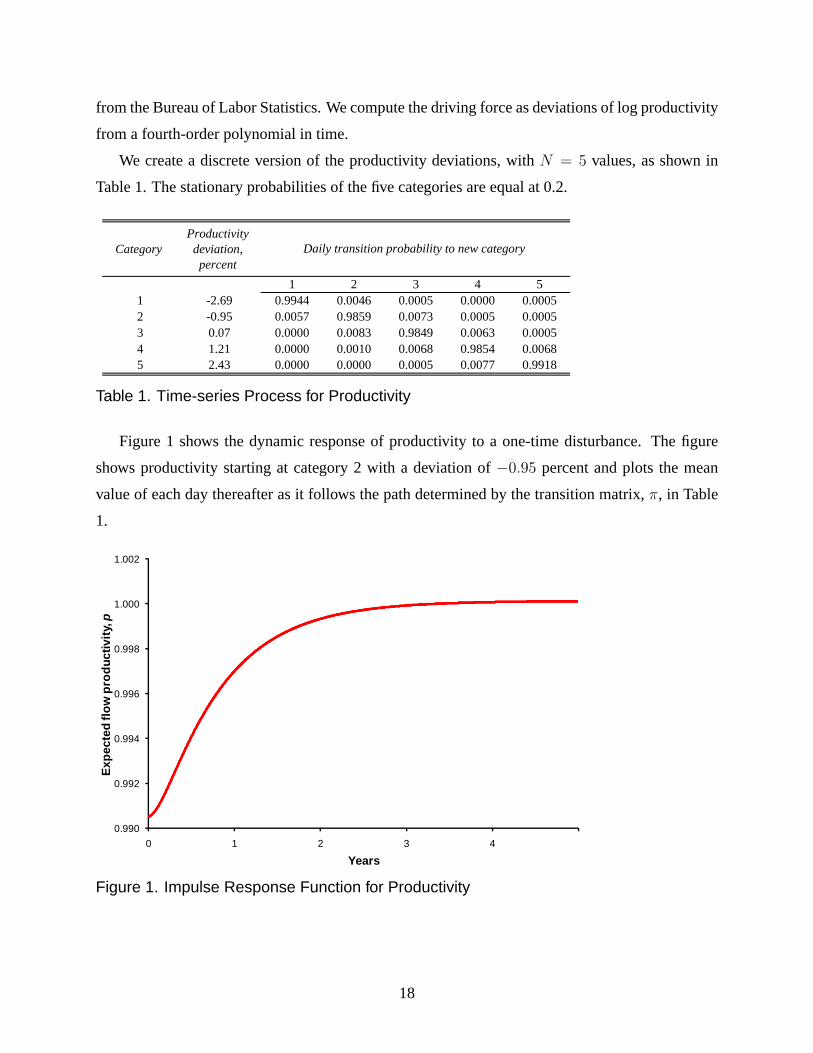
We create a discrete version of the productivity deviations, withN = 5 values, as shown in

Table 1. The stationary probabilities of the five categories are equal at 0.2.

CategoryProductivity deviation, percent

1 2 3 4 51 -2.69 0.9944 0.0046 0.0005 0.0000 0.00052 -0.95 0.0057 0.9859 0.0073 0.0005 0.00053 0.07 0.0000 0.0083 0.9849 0.0063 0.00054 1.21 0.0000 0.0010 0.0068 0.9854 0.00685 2.43 0.0000 0.0000 0.0005 0.0077 0.9918

Daily transition probability to new category

Table 1. Time-series Process for Productivity

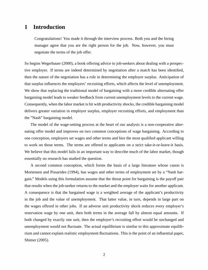
Figure 1 shows the dynamic response of productivity to a one-time disturbance. The figure

shows productivity starting at category 2 with a deviation of−0.95 percent and plots the mean

value of each day thereafter as it follows the path determined by the transition matrix,π, in Table

1.

 

 

0.990

0.992

0.994

0.996

0.998

1.000

1.002

0 1 2 3 4

Expe

cted

flow

pro

duct

ivity

, p

Years

Figure 1. Impulse Response Function for Productivity

18

3.7 Unemployment volatility attributable to productivity fluctuations

Shimer (2005) focused on the question of whether the MP model could explain the observed

volatility of unemployment as solely the result of fluctuations in productivity. Much of the re-

search his paper triggered has remained in this framework. But, as Mortensen andEva Nagypal

(2007) point out, simple econometrics shows that no reasonable model similar to the MP model

could explain all of unemployment volatility. A good deal of unemployment fluctuation is uncor-

related with productivity.

We have explored a variety of regressions of quarterly unemployment on the productivity mea-

sure just discussed. The standard deviation of the residuals from these regressions is a measure

of the component that presumptively defies explanation by productivity fluctuations. We find that

lagged productivity adds to the explanatory power. We will use a simple example that lies midway

between the specification with lowest assignment to productivity (only a single right-hand variable,

the contemporaneous productivity deviation) and the one with the highest (many lagged deviations

included as well with separate coefficients). This specification relates current unemployment to

the productivity deviation three quarters earlier.

The regression delivers the following decomposition of unemployment volatility: The standard

deviation of unemployment over the sample period, 1948 Q4 through 2007 Q1, is 1.50 percentage

points. The standard error of the residuals is 1.34 percentage points; this is the component beyond

the reach of a productivity explanation. The implied standard deviation of the component driven

by productivity is 0.68 percentage points. We will consider models that deliver this amount of

volatility when driven only by the productivity process just derived.

4 Comparison of Models

We consider three models in the generalized MP class. These are the canonical model of Mortensen

and Pissarides (1994), Hagedorn and Manovskii’s (2006) variant of the MP model with “Nash

bargaining,” and the credible-bargaining model of this paper. To facilitate the comparison, we will

standardize the non-wage parts of the model involving the matching function and the separation

rate. We will require the three models to have the same average unemployment rate of 5.5 percent.

For the MP model, we use our estimate of the flow value of non-work,z, which is higher than

Shimer and others have used. For Hagedorn and Manovskii’s model, we adopt their strategy of

choosing the value ofz from macro data. They choose it to match a measure of wage flexibility. We

19

choose it to match our measure of unemployment volatility induced by productivity fluctuations.

Later we will discuss the implications for wage flexibility.

4.1 Comparison of basic properties

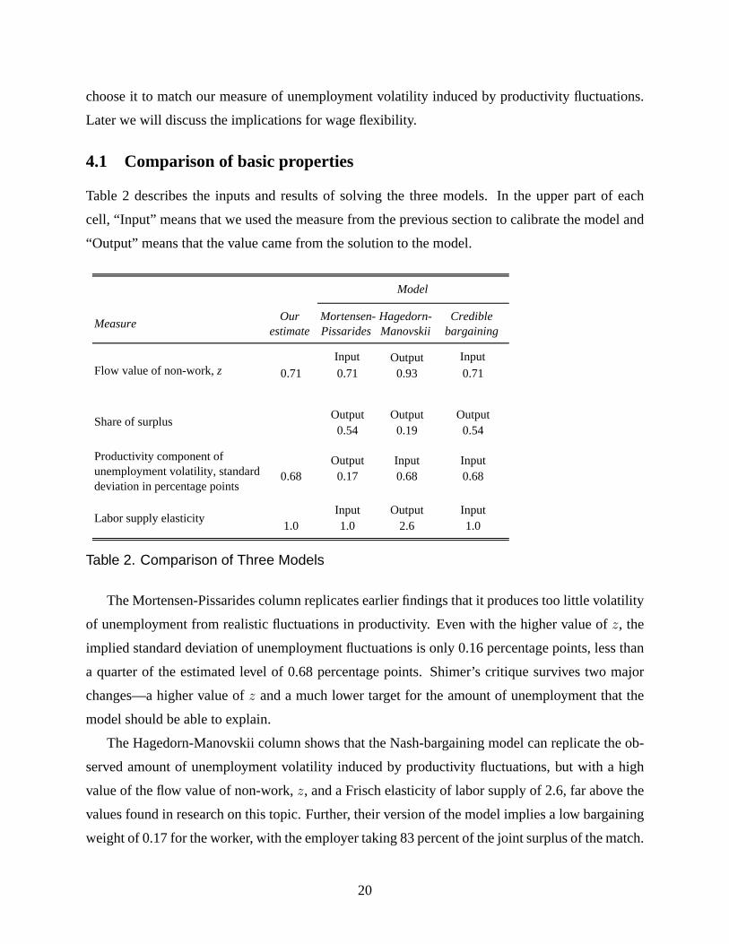
Table 2 describes the inputs and results of solving the three models. In the upper part of each

cell, “Input” means that we used the measure from the previous section to calibrate the model and

“Output” means that the value came from the solution to the model.

Measure Our estimate

Mortensen-Pissarides

Hagedorn-Manovskii

Credible bargaining

Input Output Input0.71 0.71 0.93 0.71

Output Output Output0.54 0.19 0.54

Output Input Input0.68 0.17 0.68 0.68

Input Output Input1.0 1.0 2.6 1.0Labor supply elasticity

Model

Flow value of non-work, z

Productivity component of unemployment volatility, standard deviation in percentage points

Share of surplus

Table 2. Comparison of Three Models

The Mortensen-Pissarides column replicates earlier findings that it produces too little volatility

of unemployment from realistic fluctuations in productivity. Even with the higher value ofz, the

implied standard deviation of unemployment fluctuations is only 0.16 percentage points, less than

a quarter of the estimated level of 0.68 percentage points. Shimer’s critique survives two major

changes—a higher value ofz and a much lower target for the amount of unemployment that the

model should be able to explain.

The Hagedorn-Manovskii column shows that the Nash-bargaining model can replicate the ob-

served amount of unemployment volatility induced by productivity fluctuations, but with a high

value of the flow value of non-work,z, and a Frisch elasticity of labor supply of 2.6, far above the

values found in research on this topic. Further, their version of the model implies a low bargaining

weight of 0.17 for the worker, with the employer taking 83 percent of the joint surplus of the match.

20

The credible-bargaining column shows that our model can replicate the observed volatility

of unemployment with reasonable values ofz and of the elasticity of labor supplyψ. Also, the

worker’s share of the joint surplus implied by our calibration is 0.54, which is the same as in the

MP model. Besides depending onz andγ, this share depends also on the parameterδ, the daily

probability that a job opportunity would vanish during bargaining, which we took to be 4 times the

probability that a job becomes unproductive once it starts.

4.2 Responses to Changes in Productivity

With Nash bargaining, the wage responds directly toP with a derivative equal to the bargaining

weightβ in equation (6). It responds indirectly through the presence of the opportunity cost term

(1 − β)(U − V ) in the same equation.U falls by more thanV , so the opportunity cost falls and

the wage falls on that account as well.

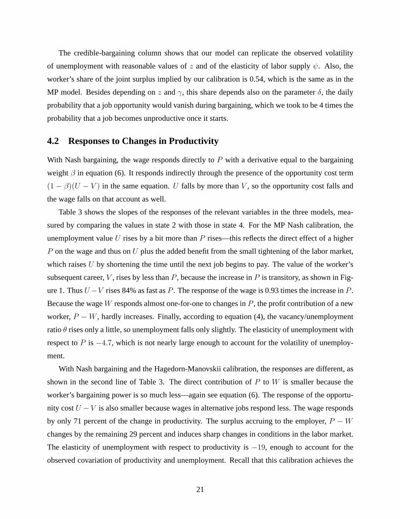
Table 3 shows the slopes of the responses of the relevant variables in the three models, mea-

sured by comparing the values in state 2 with those in state 4. For the MP Nash calibration, the

unemployment valueU rises by a bit more thanP rises—this reflects the direct effect of a higher

P on the wage and thus onU plus the added benefit from the small tightening of the labor market,

which raisesU by shortening the time until the next job begins to pay. The value of the worker’s

subsequent career,V , rises by less thanP , because the increase inP is transitory, as shown in Fig-

ure 1. ThusU−V rises 84% as fast asP . The response of the wage is 0.93 times the increase inP .

Because the wageW responds almost one-for-one to changes inP , the profit contribution of a new

worker,P −W , hardly increases. Finally, according to equation (4), the vacancy/unemployment

ratioθ rises only a little, so unemployment falls only slightly. The elasticity of unemployment with

respect toP is −4.7, which is not nearly large enough to account for the volatility of unemploy-

ment.

With Nash bargaining and the Hagedorn-Manovskii calibration, the responses are different, as

shown in the second line of Table 3. The direct contribution ofP to W is smaller because the

worker’s bargaining power is so much less—again see equation (6). The response of the opportu-

nity costU − V is also smaller because wages in alternative jobs respond less. The wage responds

by only 71 percent of the change in productivity. The surplus accruing to the employer,P −W

changes by the remaining 29 percent and induces sharp changes in conditions in the labor market.

The elasticity of unemployment with respect to productivity is−19, enough to account for the

observed covariation of productivity and unemployment. Recall that this calibration achieves the

21

Slope with respect to P Elasticity

U V W Unemploy-ment rate

Nash bargaining, Mortensen-Pissarides calibration 1.14 0.30 0.93 -4.7

Nash bargaining, Hagedorn-Manovskii calibration 0.87 0.23 0.71 -19.1

Credible bargaining 1.20 0.32 0.69 -20.0

Table 3. Responses to Changes in Productivity

realistic elasticity by making the elasticity of labor supply unrealistically high and the bargaining

power of labor low.

The credible bargaining model arrives at a similarly realistic elasticity by quite a different

route. Equation (10) is a close approximation that helps explain the responses. The wage responds

directly to a productivity change with a coefficient of 0.5.V responds by slightly more than it

does in the MP case. The increase inU is somewhat larger than in the MP case, because the labor

market tightens much more with credible bargaining. Because of the limited response toU − V ,

the wage response is only 0.69, in contrast to 0.93 in the MP-Nash case. The profit contribution,

P−W , rises substantially, stimulating recruiting effort and lowering unemployment. The elasticity

of unemployment with respect toP is−20, replicating the observed covariation of unemployment

and productivity.

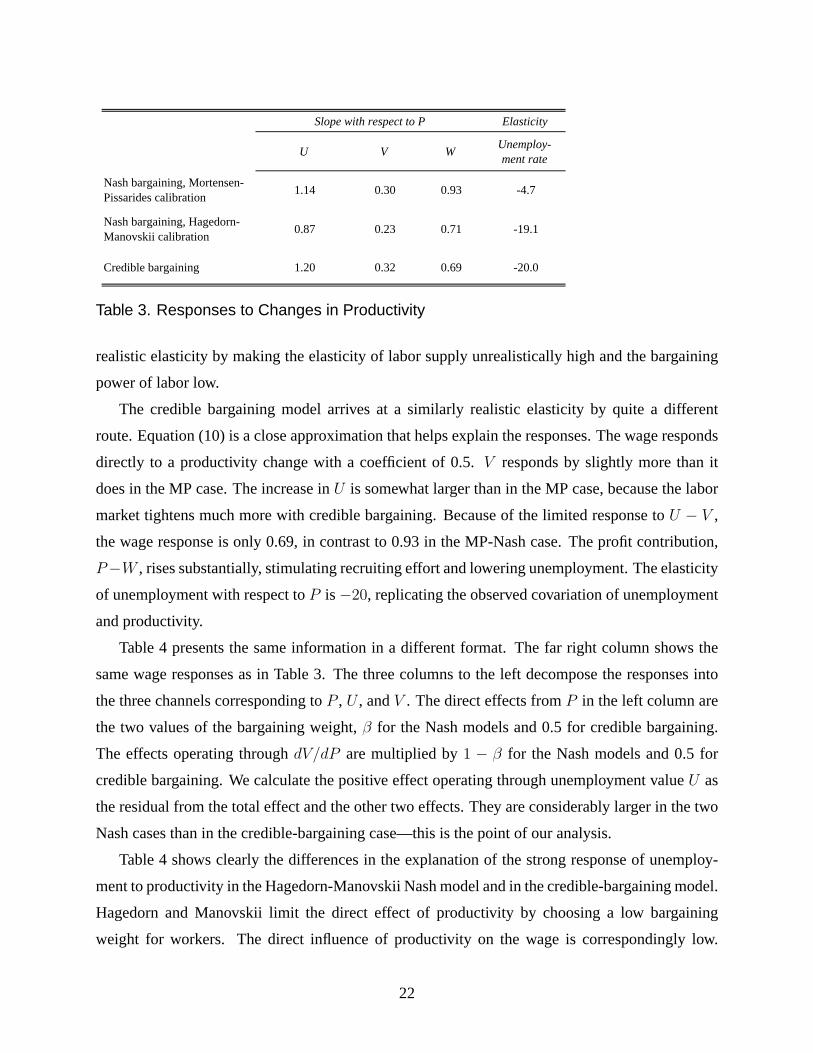
Table 4 presents the same information in a different format. The far right column shows the

same wage responses as in Table 3. The three columns to the left decompose the responses into

the three channels corresponding toP , U , andV . The direct effects fromP in the left column are

the two values of the bargaining weight,β for the Nash models and 0.5 for credible bargaining.

The effects operating throughdV/dP are multiplied by1 − β for the Nash models and 0.5 for

credible bargaining. We calculate the positive effect operating through unemployment valueU as

the residual from the total effect and the other two effects. They are considerably larger in the two

Nash cases than in the credible-bargaining case—this is the point of our analysis.

Table 4 shows clearly the differences in the explanation of the strong response of unemploy-

ment to productivity in the Hagedorn-Manovskii Nash model and in the credible-bargaining model.

Hagedorn and Manovskii limit the direct effect of productivity by choosing a low bargaining

weight for workers. The direct influence of productivity on the wage is correspondingly low.

22

Slope of P's contribution to W via

P U V

Nash bargaining, Mortensen-Pissarides calibration 0.54 0.52 -0.14 0.93

Nash bargaining, Hagedorn-Manovskii calibration 0.19 0.70 -0.18 0.71

Credible bargaining 0.50 0.35 -0.16 0.69

Slope of W with respect to P

Table 4. Decomposition of Effects of Productivity on the Wage

Their account of the influence of productivity operating thoughU andV is essentially the same as

in the MP calibration. The credible-bargaining model, by contrast, has about the same direct effect

of productivity on the wage as does the MP model but limits the role of the unemployment value

U .

5 Wage Flexibility

5.1 Measuring wage flexibility in the three models

Our results have immediate and simple implications for wage flexibility. All the models we have

discussed share the same zero-profit condition with the same parameter values. Letu = u/(1−u),the unemployment/employment ratio. The zero-profit condition can be written,

u(Pi −Wi) =cs

φ20

. (25)

Then the flexibility of wages isdW

dP= 1 +

cs

φ20u

2

du

dP. (26)

The response of the wage to productivity—the measure of wage flexibility—is directly related

to the response of unemployment to productivity. No other response appears in the derivative.

Table 4 shows that the flexibility needed to rationalize the joint movements of productivity and

unemployment is a derivative of about 0.7.

Hagedorn and Manovskii (2006) measure wage flexibility from wage and productivity data and

find a derivative of about 0.5. Although the Hagedorn-Manovskii estimate of flexibility is not too

much lower than the value implicit in our model, we are skeptical that econometric studies of wage

23

data can shed much light on the issue of unemployment volatility. The wage variableW in the

MP class of models is the employer’s expectation of the present value of wage payments over the

duration of a job, for workers about to be hired. Teasing this value out of data on wages paid to all

workers, including those hired decades ago, is a daunting exercise.

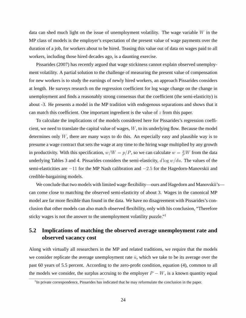
Pissarides (2007) has recently argued that wage stickiness cannot explain observed unemploy-

ment volatility. A partial solution to the challenge of measuring the present value of compensation

for new workers is to study the earnings of newly hired workers, an approach Pissarides considers

at length. He surveys research on the regression coefficient for log wage change on the change in

unemployment and finds a reasonably strong consensus that the coefficient (the semi-elasticity) is

about -3. He presents a model in the MP tradition with endogenous separations and shows that it

can match this coefficient. One important ingredient is the value ofz from this paper.

To calculate the implications of the models considered here for Pissarides’s regression coeffi-

cient, we need to translate the capital value of wages,W , to its underlying flow. Because the model

determines onlyW , there are many ways to do this. An especially easy and plausible way is to

presume a wage contract that sets the wage at any time to the hiring wage multiplied by any growth

in productivity. With this specification,w/W = p/P , so we can calculatew = pPW from the data

underlying Tables 3 and 4. Pissarides considers the semi-elasticity,d logw/du. The values of the

semi-elasticities are−11 for the MP Nash calibration and−2.5 for the Hagedorn-Manovskii and

credible-bargaining models.

We conclude that two models with limited wage flexibility—ours and Hagedorn and Manovskii’s—

can come close to matching the observed semi-elasticity of about 3. Wages in the canonical MP

model are far more flexible than found in the data. We have no disagreement with Pissarides’s con-

clusion that other models can also match observed flexibility, only with his conclusion, “Therefore

sticky wages is not the answer to the unemployment volatility puzzle.”1

5.2 Implications of matching the observed average unemployment rate andobserved vacancy cost

Along with virtually all researchers in the MP and related traditions, we require that the models

we consider replicate the average unemployment rateu, which we take to be its average over the

past 60 years of 5.5 percent. According to the zero-profit condition, equation (4), common to all

the models we consider, the surplus accruing to the employerP −W , is a known quantity equal

1In private correspondence, Pissarides has indicated that he may reformulate the conclusion in the paper.

24

to about 13 days of worker productivity. The recruiting rate is the ratio of the known job-finding

rate and the known vacancy/unemployment ratio; the flow costc is known from the sources we

discussed earlier. The amount of the employer surplus, and the counterpart surplus accruing to

workers, controls important features of the calibration of the rest of the model. We do not think it

would be appropriate to adopt a calibration that failed to match the observed value ofP −W .

Among Nash-bargaining models, fixing the known value ofP − W , matchingu creates a

tradeoff between the two parameters controlling unemployment, the flow valuez and bargaining

powerβ. Our MP calibration withz = 0.71 andβ = 0.54 is one point on that tradeoff and our

Hagedorn-Manovskii calibration withz = 0.93 andβ = 0.19 is another. In the credible-bargaining

model, the corresponding tradeoff is betweenz and the employer’s delay costγ. Given our belief

thatz = 0.71 is known from research on labor supply and consumption, the implied value ofγ is

0.27 days of worker compensation per day of delay. The reasonableness of this cost provides some

confirmation of the model itself.

The sum ofz andγ is 0.98, not very different from the value ofz by itself in our version

of Hagedorn and Manovskii’s calibration, namely 0.93. One might conclude that the credible

bargaining model is really the same as their model, with a different rationalization for the same

value ofz + γ. It is true, as we noted above, thatz + γ controls the unemployment rate, so if

we believed in a higherz, we would need to believe in a lowerγ, but this sum alone does not

determine unemployment volatility. In the credible-bargaining model, volatility is also controlled

by the frequency of bargaining interruptions,δ. The fact that the Hagedorn-Manovskii value of

z corresponds to aγ of zero in our model is essentially unrelated to the fact that our model and

theirs imply equal values of unemployment volatility. For example, the credible-bargaining model

with δ = 0 implies much higher unemployment volatility, but still hasz+γ close to Hagedorn and

Manovskii’sz.

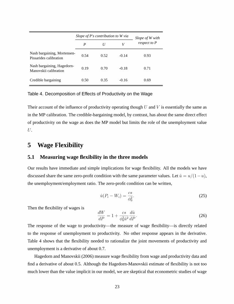
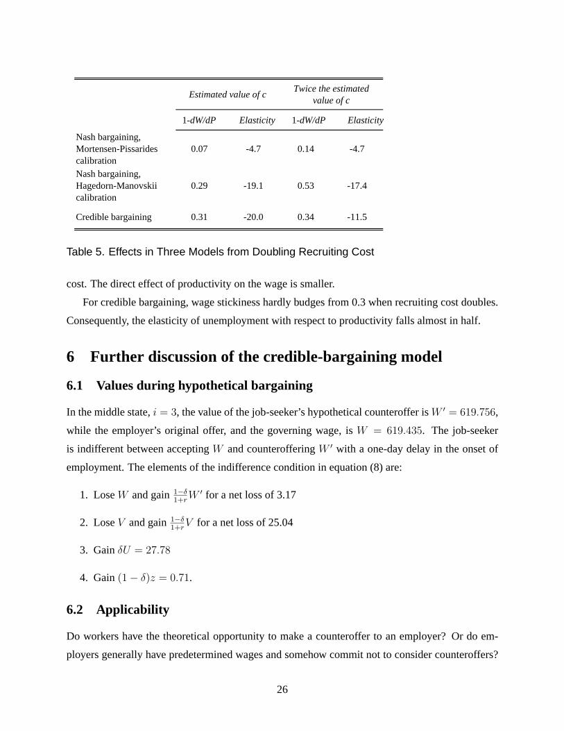
The properties of the models depend on the vacancy costc. We compare the estimated value of

c to a value twice as high. According to equation (26), this cuts the relation between the response of

unemployment,dudP

, and the stickiness of the wage,1− dWdP

, in half. Table 5 compares the changes

in the three models upon the doubling ofc.

For both Nash-bargaining calibrations, the higher recruiting cost roughly doubles wage stick-

iness. This effect largely offsets the halving of the multiplier relating wage stickiness to the em-

ployment response, so the latter declines only a little. The reason that the Nash calibration has less

flexible wages with higher recruiting cost is that the worker’s bargaining share is lower for higher

25

Estimated value of c Twice the estimated value of c

1-dW/dP Elasticity 1-dW/dP Elasticity

Nash bargaining, Mortensen-Pissarides calibration

0.07 -4.7 0.14 -4.7

Nash bargaining, Hagedorn-Manovskii calibration

0.29 -19.1 0.53 -17.4

Credible bargaining 0.31 -20.0 0.34 -11.5

Table 5. Effects in Three Models from Doubling Recruiting Cost

cost. The direct effect of productivity on the wage is smaller.

For credible bargaining, wage stickiness hardly budges from 0.3 when recruiting cost doubles.

Consequently, the elasticity of unemployment with respect to productivity falls almost in half.

6 Further discussion of the credible-bargaining model

6.1 Values during hypothetical bargaining

In the middle state,i = 3, the value of the job-seeker’s hypothetical counteroffer isW ′ = 619.756,

while the employer’s original offer, and the governing wage, isW = 619.435. The job-seeker

is indifferent between acceptingW and counterofferingW ′ with a one-day delay in the onset of

employment. The elements of the indifference condition in equation (8) are:

1. LoseW and gain1−δ1+r

W ′ for a net loss of 3.17

2. LoseV and gain1−δ1+r

V for a net loss of 25.04

3. GainδU = 27.78

4. Gain(1− δ)z = 0.71.

6.2 Applicability

Do workers have the theoretical opportunity to make a counteroffer to an employer? Or do em-

ployers generally have predetermined wages and somehow commit not to consider counteroffers?

26

We have been unable to findanyacademic empirical literature on the process by which employers

and job-seekers arrive at the terms of employment. Because our model makes the unambiguous

prediction that counteroffers do not occur in equilibrium, there is no use in asking if workers make

counteroffers in reality. We believe that a commitment not to consider counteroffers is difficult to

achieve.

Our impression of the process of wage determination—not founded on any extensive body

of systematic empirical evidence—is that job-seekers gather information from friends and help-

wanted ads, and they post resumes on websites to find jobs for which they are well matched. An

employer reviews information about applicants and searches databases for good matches. The

employer calls in the more promising prospects for interviews. Having found what appears to be

a good match, the employer makes a comprehensive job offer, including pay, benefits, and duties.

We believe that employers almost always make the initial offer. Many job-seekers accept the initial

offer, but others make counteroffers. The probability that the job-seeker and employer will make

an acceptable deal is high, once the employer has decided to make the initial offer.

Our model is a stylized representation of this process. We do not try to model the directed

nature of the search—in our model, job-seekers know nothing about a job. And there is nothing

to know because all jobs are alike. We concentrate on one realistic aspect—one party starts the

process by making an offer and the other can then accept or respond with a counteroffer. The

unique equilibrium in our model is for acceptance of the initial offer. Thus the model is successful

in explaining why few job-seekers make counteroffers (if that is true) but not successful in explain-

ing why some job-seekers do make counteroffers. Models with information asymmetries might be

able to explain the latter.

7 Other Research Relevant to the Wage Bargain

7.1 The alternating offer bargaining model

Infinite horizon, alternating offer bargaining models were introduced into economics by Rubinstein

(1982) and have spurred a very large literature. Rubinstein and Wolinsky (1985) incorporate search

and bargaining in a non-stochastic model and find that market outcomes may be far from the

competitive equilibrium even when search costs and search times are vanishingly small. Gale

(1986) introduces the possibility that the arrival of other parties may interrupt bargaining and create

an auction; he shows that this structure reverses the Rubinstein-Wolinsky conclusion. Osborne and

Rubinstein (1990) give an integrated review of the early literature.

27

Binmore et al. (1986) first developed the distinction between a threat point and an outside

option in their alternating offer bargaining model. Binmore, Shaked and Sutton (1989) report lab-

oratory experiments that affirm the importance of this distinction. Malcomson (1999) argues for

its importance in analyzing labor contracts, while a number of others have applied the BRW theory

to individual wage determination. These include Rosen (1997), Shimer (2005), Menzio (2005),

and Delacroix (2004). None of these papers deals with our topic, the way that alternating-offer

bargaining delivers substantial employment fluctuations. Delacroix investigates sticky wages and

employment fluctuations, but in a setting without unemployment or pre-match non-contractible

recruiting effort by employers. In his model, wages are sticky during the course of employment.

Employment fluctuations arise from bilaterally efficient endogenous separations, not from varia-

tions in recruiting effort, as in our model and others in the MP tradition based on sticky wages as

of the time the employment match is formed.

7.2 Mortensen and Nagypal’s version of the model

Mortensen andEva Nagypal (2007) and Mortensen (2007) cite this paper in support of a simple

wage bargain where the wage is the equally weighted average of the flow value of non-work,z,

and productivityp. Their conclusion follows from our equation (10) in a static setting with the cost

of bargaining to the employer,γ, set to zero. They observe, as our model implies, that the response

of the wage to productivity delivers reasonably substantial unemployment volatility.

As we explained earlier in section 4.1, we believe it is inappropriate to adopt a calibration

that does not match the observed average unemployment rate. The Mortensen-Nagypal calibration

either fails to match the data we cite on the cost of maintaining a vacancy or it fails to match the

average unemployment rate. But their calibration does not miss these targets by much and we find

it congenial to the main point of this paper.

8 Competing Opportunities During Bargaining

So far, we have assumed that as the worker and employer negotiate, they are never interrupted by

another competitor—a worker or employer. How might allowing new arrivals during negotiations

alter our analysis?

Rubinstein and Wolinsky (1985) found negotiated prices far from competitive equilibrium even

when search frictions are small in an alternating offer bargaining model. Gale (1986) modified

their model to allow arrivals of additional players during bargaining and assumed that new arrivals

28

trigger an auction. In the labor market context, if the newly arriving bargainer were a worker

and the two workers bid in an auction for the single job, then the losing bidder would return to

unemployment, which paysU . Then, Bertrand competition would also limit the winning bidder

to a payoff ofU , tying the equilibrium wage tied tightly to the unemployment payoff. If the new

arrival were another employer, Bertrand competition between the two employers would give the

worker the entire surplus.

We study the two cases separately. In the case of two workers bidding for the same job, the

basic structure of the Mortensen-Pissarides model permits a simple argument that the auction will

have the same equilibrium wage as bilateral bargaining. Employers create jobs costlessly, apart

from a recruiting cost. An employer cannot commit not to bargain with the loser of the auction,

because the bargain will yield a positive value to the employer, as in our earlier analysis. The

bids in the auction will reflect the knowledge that the loser gets the bargained wage. Hence the

equilibrium of the auction is the bargained wage, and the auction possibility has no effect on our

earlier conclusions.

The case of two employers bidding for the same worker is quite different. The losing employer

returns to recruiting—there is no alternate worker standing in the wings, comparable to the alter-

nate job in the previous case. The lucky worker receives a wage equal to productivity and the

winning employer receives no part of the surplus. The result is to connect the wage to productivity,

not to make the unemployment valueU a direct determinant of the wage. However, labor-market

conditions have a larger role in wage determination because they control the probability that a

second employer will appear during bargaining.

It should not be taken for granted that a job-seeker can run an auction where two employers

make competing bids. We have found no empirical literature studying how bargaining takes place

in labor markets, but casual empiricism suggests that for many types of jobs, auctions among

employers for a worker are not common.

One practical reason that auctions for a worker do not occur is that an employer cannot verify

the bid of another employer. The worker’s representation about a competing opportunity is cheap

talk and it is hardly in the employer’s interest to confirm the worker’s claim. If no auction is

available, the best the worker can do is to pick the employer where the bilateral bargain is most

favorable and make that bargain.

Even when wage offers are common knowledge among the parties, the equilibrium depends on

the bargaining protocol. Consider the following bargaining game, which we believe may govern

29

important parts of the labor market. When it is the worker’s turn to make an offer, she can abandon

bargaining with the first-to-arrive employer and instead make an offer to the second employer,

leaving the first employer to return to recruiting.

In this game, when the worker abandons bargaining with the first employer, she enters a sub-

game that is identical to the bargaining game we have analyzed above, leading to a worker’s payoff

of W + V . So, we can analyze the subgame perfect equilibria of the new game by replacing the

subgame with a terminal node at which the worker is assigned a payoff ofW + V . That payoff

functions as an outside option for the worker—an amount that she can claim if she stops bargaining

with the first employer. By the BRW logic, this outside option does not affect the agreement with

the first employer: the worker cannot credibly threaten to refuse a deal today payingW + V and

terminate negotiations today in favor of a deal paying the same amount tomorrow. Hence, in this

model, the wage bargain is unaffected by the arrival of a new job applicant.

The same conclusion applies for any model in which the worker can switch back and forth a

maximum ofN times, whereN is any positive integer. This follows by induction: Suppose that

the worker’s unique equilibrium payoff isW + V in any game where it can switchN − 1 times.

Then, just as above,W + V is the employer’s outside option in the initial negotiation with the

first-to-arrive worker and the conclusion follows.

Binmore (1985) analyzed a similar “telephone bargaining” model, but with no limitN on the

number of times the bargainer can switch back and forth between the employers. He found that

the same offer policies emerge at one equilibrium. The uniqueness argument made above was

written to apply to this game as well; it proves that the equilibrium wage offerW is unique. The

equilibrium itself is not unique. Indeed, there are infinitely many subgame perfect equilibria, but

they vary only in the way the worker chooses a bargaining partner whenever she faces that choice.

Of course, we do not believe that competition from other applicants for a job or other jobs

available to a worker is actually as limited as the characterization in our model. Not every employer

has a second job ready when two qualified applicants appear at the same time for one job. In some

cases, competing offers to the same applicant can be verified, so a worker can run an auction.

Perhaps in some cases workers can put competing employers in the same room and make them bid

directly against each other. Our point is that there are good reasons to think that these situations

are not the rule and that the rule is bilateral alternating-offer bargaining.

30

9 Concluding Remarks

The process by which workers and employers reach agreement on the terms of employment is a key

determinant of real-wage rigidity and has first-order implications for the volatility of unemploy-

ment. If the parties believe that rejecting an offer results in an immediate return to unemployment,

then the wage is naturally sensitive to conditions in the labor market. But the belief that the only

alternative to accepting an offer is to return to unemployment is wrong; the parties can instead sim-

ply continue to bargain. When two well-matched parties recognize that one side cannot credibly

refuse to consider a counteroffer, conditions in the outside labor market have much less influence

on the wage bargain.

In the standard Mortensen-Pissarides model, if unemployment were to become high, the re-

sulting fall in wages would stimulate labor demand and excess unemployment would vanish. With

credible wage bargaining, however, the limited influence of unemployment on the wage results in

large fluctuations in unemployment under plausible movements in the driving force.

31

References

Anderson, Patricia M. and Bruce D. Meyer, “Unemployment Insuracne Takeup Rates and the

After-Tax Value of Benefits,”Quarterly Journal of Economics, August 1997,112 (3), 913–

937.

Binmore, Ken, “Bargaining and Coalitions,” in A. Roth, ed.,Game-Theoretic Models of Bargain-

ing, Cambridge: Cambridge University Press, 1985.

, Ariel Rubinstein, and Asher Wolinsky, “The Nash Bargaining Solution in Economic Mod-

eling,” RAND Journal of Economics, Summer 1986,17 (2), pp. 176–188.

, Avner Shaked, and John Sutton, “An Outside Option Experiment,”Quarterly Journal of

Economics, 1989,104(4), pp. 753–770.

Coles, Melvyn G. and Randall Wright, “A Dynamic Equilibrium Model of Search, Bargaining,

and Money,”Journal of Economic Theory, 1998,78, pp. 32–54.

Delacroix, Alain, “Sticky Bargained Wages,”Journal of Macroeconomics, 2004,26, 25–44.

Gale, Douglas, “Bargaining and Competition, Part I: Characterization,”Econometrica, 1986,54

(4), pp. 785–806.

Hagedorn, Marcus and Iourii Manovskii, “The Cyclical Behavior of Equilibrium Unemployment

and Vacancies Revisited,” April 2006. University of Frankfurt and University of Pennsylva-

nia.

Hall, Robert E., “Employment Fluctuations with Equilibrium Wage Stickiness,”American Eco-

nomic Review, March 2005,95 (1), 50–65.

, “Job Loss, Job Finding, and Unemployment in the U.S. Economy over the Past Fifty Years,”

NBER Macroeconomics Annual, 2005. Forthcoming.

, “Sources and Mechanisms of Cyclical Fluctuations in the Labor Market,” July 2007. Hoover

Institution, Stanford University, www.Stanford.edu/∼rehall.

Holden, Steinar, “Wage Bargaining, Holdout, and Inflation,”Oxford Economic Papers, 1997,49,

235–255.

32

Krueger, Alan B. and Bruce D. Meyer, “Labor Supply Effects of Social Insurance,” in Alan Auer-

bach and Martin Feldstein, eds.,Handbook of Public Economics, Volume 4, Elsevier, 2002,

pp. 2237–2392.

Malcomson, James M., “Individual Employment Contracts,” in Orley Ashenfelter and David Card,

eds.,Handbook of Labor Economics, Vol. 3B, New York: North Holland, 1999, chapter 35,

pp. 2291–2372.

Menzio, Guido, “A Cheap-Talk Theory of Random and Directed Search,” September 2005. De-

partment of Economics, University of Pennsylvania.

Mortensen, Dale T., “Island Matrching,” June 2007. Northwestern University.

and Christopher Pissarides, “Job Creation and Job Destruction in the Theory of Unemploy-

ment,”Review of Economic Studies, 1994,61 (0), pp. 397–415.

andEva Nagypal, “More on Unemplohyment and Vacancy Fluctuations,”Review of Eco-

nomic Dynamics, 2007,10, 327–347.

Osborne, Martin and Ariel Rubinstein,Bargaining and Markets, New York: Academic Press,

1990.

Petrongolo, Barbara and Christopher A. Pissarides, “Lookin into the Black Box: A Survey of the

Matching Function,”Journal of Economic Literature, June 2001,39 (2), 390–431.

Pissarides, Christopher, “The Unemployment Volatility Puzzle: Is Wage Stickiness the Answer?,”

June 2007. Walras-Bowley Lecture, North American Summer Meetings of the Econometric

Society.

Rosen, Asa, “An Equilibrium Search-Matching Model of Discrimination,”European Economic

Review, 1997,41, 1589–1613.

Rubinstein, Ariel, “Perfect Equilibrium in a Bargaining Model,”Econometrica, 1982,50 (1), pp.

97–110.

and Asher Wolinsky, “Equilibrium in a Market with Sequential Bargaining,”Econometrica,

1985,53 (5), pp. 1133–1150.

33

Shimer, Robert, “The Cyclical Behavior of Equilibrium Unemployment and Vacancies,”American

Economic Review, 2005,95 (1), 24–49.

Silva, Jose A. and Manuel Toledo, “Labor Turnover Costs and the Cyclical Behavior of Vacancies

and Unemployment,” February 2007. Universitat Autonoma de Barcelona and Universidad

Carlos III de Madrid.

Wegerbauer, Maryanne L.,Job Offer! A How-To Negotiation Guide, Indianapolis: Jist Publishing,

2000.

34

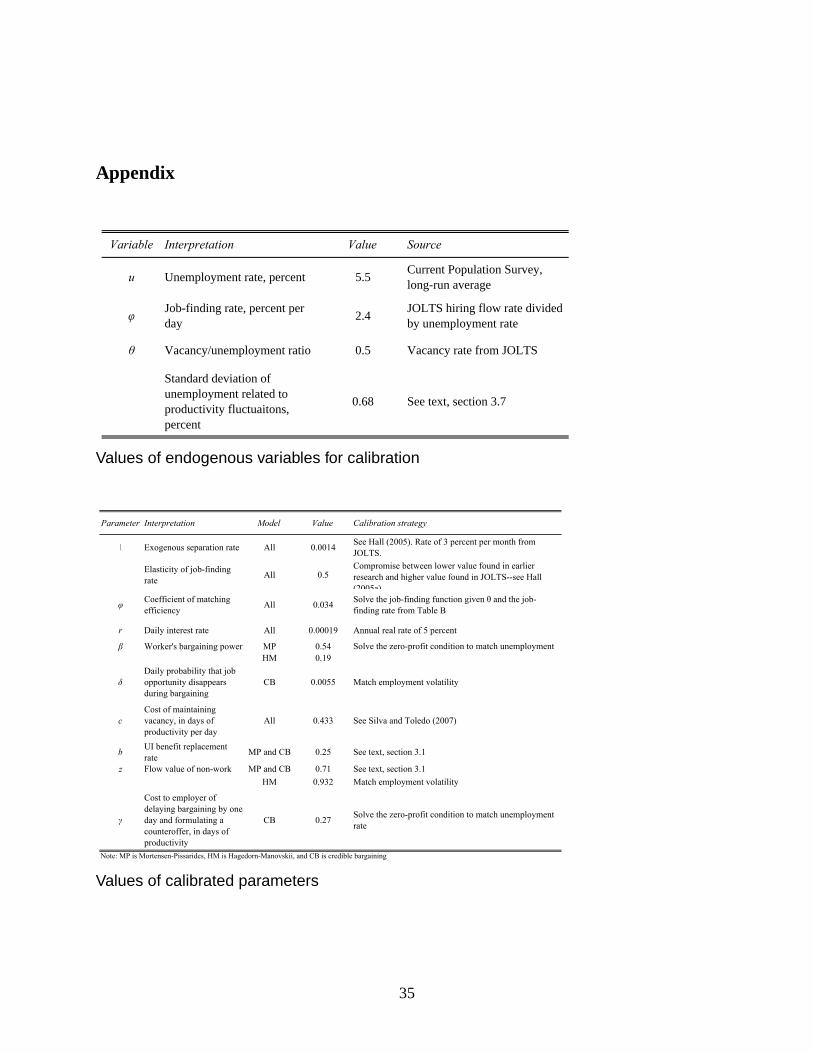
Appendix

Variable Interpretation Value Source

u Unemployment rate, percent 5.5 Current Population Survey, long-run average

φ Job-finding rate, percent per day 2.4 JOLTS hiring flow rate divided

by unemployment rate

θ Vacancy/unemployment ratio 0.5 Vacancy rate from JOLTS

Standard deviation of unemployment related to productivity fluctuaitons, percent

0.68 See text, section 3.7

Values of endogenous variables for calibration

Parameter Interpretation Model Value Calibration strategy

\ Exogenous separation rate All 0.0014 See Hall (2005). Rate of 3 percent per month from JOLTS.

Elasticity of job-finding rate All 0.5

Compromise between lower value found in earlier research and higher value found in JOLTS--see Hall (2005a)

φ Coefficient of matching efficiency All 0.034 Solve the job-finding function given θ and the job-

finding rate from Table B

r Daily interest rate All 0.00019 Annual real rate of 5 percent

β Worker's bargaining power MP 0.54 Solve the zero-profit condition to match unemployment HM 0.19

δDaily probability that job opportunity disappears during bargaining

CB 0.0055 Match employment volatility

cCost of maintaining vacancy, in days of productivity per day

All 0.433 See Silva and Toledo (2007)

b UI benefit replacement rate MP and CB 0.25 See text, section 3.1

z Flow value of non-work MP and CB 0.71 See text, section 3.1HM 0.932 Match employment volatility

γ

Cost to employer of delaying bargaining by one day and formulating a counteroffer, in days of productivity

CB 0.27 Solve the zero-profit condition to match unemployment rate

Note: MP is Mortensen-Pissarides, HM is Hagedorn-Manovskii, and CB is credible bargaining

Values of calibrated parameters

35