The Limits of Adiabatic Quantum Computation

Alper Sarikaya

June 11, 2009

Presentation of work given on:

Thesis and Presentation approved by:

Date:

Contents

Abstract ii

1 Introduction to Quantum Computation 11.1 Mechanics of a Quantum Computer . . . . . . . . . . . . . . . . . . . . . . . 11.2 Qubits . . . . . . . . . . . . . . . . . . . . . . . . . . . . . . . . . . . . . . . 31.3 Adiabatic Quantum Computation . . . . . . . . . . . . . . . . . . . . . . . . 4

1.3.1 Adiabatic Evolution . . . . . . . . . . . . . . . . . . . . . . . . . . . 51.4 NP-Complete Problems and Quantum Computers . . . . . . . . . . . . . . . 6

1.4.1 Adiabatic Efficiency . . . . . . . . . . . . . . . . . . . . . . . . . . . 8

2 Adiabatic Quantum Simulation on a Classical Computer 92.1 The Simplest Case . . . . . . . . . . . . . . . . . . . . . . . . . . . . . . . . 102.2 Experimental Setup . . . . . . . . . . . . . . . . . . . . . . . . . . . . . . . . 112.3 Example of a Sample Run . . . . . . . . . . . . . . . . . . . . . . . . . . . . 112.4 Simulation of an Example Adiabatic Algorithm . . . . . . . . . . . . . . . . 13

3 Conclusions and Future Work 143.1 Possible Effects to Adiabatic Quantum Computing . . . . . . . . . . . . . . 143.2 Ongoing and Future Work . . . . . . . . . . . . . . . . . . . . . . . . . . . . 163.3 Acknowledgements . . . . . . . . . . . . . . . . . . . . . . . . . . . . . . . . 16

Bibliography 17

i

Abstract

Quantum computation has long been known to offer an exponential speed-up overclassical computational algorithms for some algorithmic problems. Quantum algo-rithms evolve by repeatedly applying an infinitesimal operator, the Hamiltonian, tothe initial state and end in a final quantum state. Adiabatic quantum computationis one of many quantum methods that utilize the properties of quantum mechanics inorder to arrive at a final solution (or more correctly, state). The qualifier adiabatic isneeded to show that this class of algorithms is perpetuated by a simple Hamiltonianthat never gets excited past the ground state. In this project, we am investigating alarge class of adiabatic algorithms to elucidate the magnitude of the speed-up betweenthem and classical algorithms, demonstrating that this class of adiabatic quantumalgorithms does not offer an exponential increase in efficiency. Based on previous ob-servations, we postulate that efficiency increase of adiabatic quantum algorithms overclassical ones are limited to just a polynomial speed-up for a specific set of adiabaticalgorithms. This hypothesis was confirmed by simulating an adiabatic algorithm clas-sically, and comparing the real-time efficiency of it to the theoretical runtime of theadiabatic quantum computation. We have shown this to be true for a simple caseand are currently working on demonstrating the polynomial effect for a Markovianoperator (utilizing two time-dependent Hamiltonians). In doing so, the goal is two-fold: (1) we hope to disprove the evidence that some adiabatic quantum algorithmsoffer a exponential speed-up over their classical counterparts and (2) present quantumcomputation in a manner that is simple and straightforward manner for the generaluniversity community.

ii

Chapter 1

Introduction to QuantumComputation

1.1 Mechanics of a Quantum Computer

Quantum computation is the study of a futuristic computing system where the units of

memory, quantum binary bits (or more concisely, qubits), have quantum properties that give

a computational advantage over classical computing systems. Though a practical, working

quantum computer has not been created, the theory of the field is dense and evolving, ready

for the engineering of this new type of computer.

The theory for quantum computation follows from probabilistic computing, where a cer-

tain number of bits can represent all combinations of the number of bits, each state with

a probability associated with it. Classical computation, on the other hand, is determinis-

tic, meaning that only one state is possible (probability that a specific state is represented

by the bits is one). Quantum computation utilizes the inherent advantages of probabilistic

computation of state superposition and pairs it with complex numbers. By representing

bits in the quantum world as complex numbers, computation moves from the L1-norm in

classical computation where operations strictly use stochastic matrices, which preserve that

all probablities add up to one, to the L2-norm, which uses unitary matrices. Utilizing uni-

tary matrices ensures that the sum of the squares of the input vector sum to one, allowing

1

rotational transformations of quantum states – theoretically allowing quantum computation

to be much more powerful over our current classical computers [6, 7].

The theory of quantum computation depends on the evolution of a system from its initial

state to a ground state of its operator, the Hamiltonian. The lowest energy state, or the

ground state, will represent an answer to the given problem defined by the specific Hamilto-

nian operator that embodies the algorithmic goals of the computation. The computational

system in this case embodies all parts of the computation: the initial vector (parameters of

the problem) and the process of evolving the initial vector by repeatedly applying the Hamil-

tonian operator to the vector. Utilizing the Hamiltonian as an operator on a wavefunction,

eigenvectors and eigenvalues will be generated that will relate the original wavefunction to

the new, computed wavefunction. Both the eigenvalue and the eigenvector make up the

eigenstate of the quantum algorithm at any point in time [1, 4, 7].

From each evolution step, the eigenstate of the system changes. A quantum algorithm

arrives at the final computed answer when the energy of the system is minimized. The

energy of a particular eigenstate is defined by its eigenvalue, while the eigenvector is the

final state of the algorithm. Therefore, to successfully run a quantum algorithm, an easy

to construct initial wavefunction and an appropriately picked operator needs to be evolved

until a ground state is discovered. This ground state is probabilistic and exists only in the

quantum world – to get a classical result, the eigenstate must be measured. Doing so will

collapse the superposition of states, each state with a certain probability, into a single state

that will be seen by the observer [6]. This has the effect of killing off any further quantum

computation as the superposition of eigenvectors has been collapsed into a single state, so

the decision to measure an eigenstate must be done with care.

Through these computations and operations, it is visible that although complex numbers

are involved, the mathematics required to simulate and construct a quantum system are

not more advanced than linear algebra - matrices as wavefunctions (ψ) and operators (H)

2

are prevalent throughout quantum computational theory. It should be noted, however, that

quantum theorists have adopted the bra-ket notation (also known as Dirac notation, example:

〈x|ψ〉 = ψ(x)), which can be generalized down to the inner product of all terms involved.

This restricts the bra, or the first part of the notation to be the conjugate transpose of the

ket, the second part [6]. This notation is used throughout the paper.

It has already been hinted that there is some sort of state that is propagated when

applying a Hamiltonian operator repeatedly. This state is stored in a quantum binary digit,

commonly abbreviated as qubit.

1.2 Qubits

Qubits have several quaint features that set them apart from classical (digital) bits. The

first is a direct allegory from the realm of analog (probabalistic) bits – a qubit can reside in

any fractional state between zero and one. This, on its own, allows a quantum bit to store

more information than a classical bit as individual qubits can represent nearly any linear

combination of two possible states while the classical bits are limited to simply on or off.

Secondly, qubits are allowed to be in a superposition of states and be two or more sources

of information at a time. However, this feature imposes a restriction on the observation of

a qubit: a qubit can evolve through a computation while maintaining this superposition,

but as soon as an answer or low-energy state is achieved, measurement of the qubit will

force the collapse of the stacked states into one of the superpositioned states with that

state’s probability p [6, 7]. This ramification of qubit superposition can be thought as an

observation from the famous quantum thought experiment of Schrodinger’s cat. Lastly,

qubits can entangle with one another, wherein a transition of one of two spatially separated

qubits has an effect on the other. This, thereby, allows the transmission and dissemination of

information between qubits without wires and gives the additional advantage of parallelism

3

to the computation.

We have already stated that a qubit in its ground state (lowest energy state) will most

likely, after quantum evolution, yield an answer with a high probability, when measured.

To assist in getting the right answer the first time, multiple qubits can be used in parallel

for the same computation. The measurement will yield as many answers as qubits, and the

statistically highest probability, the lowest energy state, should show up the most times [6].

Though the theory of qubits in their computation and properties have been well es-

tablished, the practicality of simulating them in the real world has been challenging. Due

to environmental temperature, it is difficult to sustain a qubit for any time longer than a

second before quantum decoherence takes hold. Decoherence stems from the insufficient

separation between the quantum system and the surrounding environment, which will cause

a non-unitary transition, effectively destroying any quantum properties of the qubits in the

system, and is one of the factors that limits the real, practical use of quantum computers

[1].

1.3 Adiabatic Quantum Computation

Even though a quantum computer has so far been described as a very general system,

an adiabatic quantum computer has some very specific limitations, making the field both

practically promising and potentially computationally limiting. Instead of allowing a system

to evolve into nearly arbitrary states and energies, the adiabatic restriction ensures that

the Hamiltonian operator is local: interactions and evolutions are restricted to a constant

number of particles, making a physical representation of an adiabatic quantum computer

possible and more feasible as there is now a restriction of finite particles to describe the

system [5].

4

1.3.1 Adiabatic Evolution

Again, a quantum system evolves according to the Schrodinger equation:

id

dt= |ψ(t)〉 = H(t)|ψ(t)〉 (1.1)

Adiabatic Hamiltonians need to be at least one-parameter operators to allow the adiabatic

(low-energy) variations to occur. At t = 0, |ψ(0)〉 is the ground state of H(0). This ground

state can be described as

|ψ(0)〉 = |l = 0; s = 0〉, (1.2)

where l and s are the instantaneous eigenstates and eigenvalues of Hi(t). If we define T

to be the upper-bound of the time parameter, a parameter s can be defined as t/T , which

we will use henceforth. It has been stated that the eigenvalues of a particular eigenstate

describe the simultaneous energy of the eigenstate - the adiabatic theorem ensures that the

gap between the two lowest energy levels E1(s)−E0(s) is always strictly positive. Since this

is the case,

limT→∞

|〈l = 0; s = 1|ψ(T )〉| = 1 (1.3)

Since there is a distinct eigenvalue gap, a wavefunction |ψ(t)〉 obeying the Schrodinger

equation will remain close to the instantaneous ground state of the current Hamiltonian H(t)

for all t from 0 to T , given T is large enough. The eigenvalue gap has been mentioned; it is

defined here:

gmin = min0≤s≤1

(E1(s)− E0(s)) (1.4)

All that is done here is smoothly varying the parameter s until the smallest eigenvalue

5

gap is found. This smallest eigenvalue signifies the presence of a ground state, and henceforth

the result of the adiabatic quantum algorithm [1, 2, 3, 4].

An adiabatic quantum algorithm consists of two Hamiltonians: the first is a (usually

simple) Hamiltonian with an easy to construct or known ground state. This initial one-

parameter Hamiltonian (known henceforth in this paper as Hi(t)) is coupled with a final

Hamiltonian Hf that has a computationally-challenging ground state. Combining these two,

the computational Hamiltonian is defined as

H(s) = (1− s)Hf + sHi, (1.5)

which can also be expressed as

H(t) = (1− t/T )Hf + (t/T )Hi (1.6)

for some fixed, large T . The quantum evolution is started at s = 0 where the ground state

of H(0) is known (since the ground state of Hi(0) is well-known) and evolved according to

the Schrodinger equation for time T [1, 4].

1.4 The Ability of Quantum Computers to Solve NP-

Complete Problems

When discussing the advantages of a quantum computer, invariably one of the major gains

is the apparent polynomial-time solving of NP-complete problems. The algorithmic speedup

gained widespread attention in 1994 with Peter Shor’s discovery of a polynomial-time prime

factoring algorithm. While the best-known classical algorithm for obtaining prime factors

from a large number works on an sub-exponential timescale, Shor’s algorithm will run in

worst-case polynomial-time [6, 7]. This has large implications both in the security and

theory worlds of computer science. In terms of security, more efficient factorization can

6

break public-key cryptography such as the widely-used RSA, which depends on factorization

being infeasible due to algorithmic complexity. Many of the most secure systems on the

internet depend on RSA for encrypted communication between two parties - breaking it

would have huge ramifications on how the internet and its cryptosystems are designed.

However, we are more excited with the prospect that it brings to the theory side of

computer science. With this increase in efficiency, the question is raised whether this applies

to the famous class of problems known as NP-complete [3]. There are numerous problems

that fall within this class - anything from useful results of the Traveling Salesman problem

(path optimization) to the Boolean satisfiability problem (SAT) to graph coloring; all of

which are incredibly important problems in computer science and beyond, but with no real

obvious efficient algorithm or procedure to generate a complete solution [2]. A solution can

be easily verified, but the generation of the solution is the most difficult part. All NP-

complete problems can be reduced to the same problem, so it follows that if a more efficient

solution is found for the satisfiability problem, all NP-complete problems can also benefit

from the efficacy increase [2].

The integer factorization problem discussed initially has been qualified into the class

of problems abbreviated BQP for “bounded error, quantum, polynomial time.” This class

encompasses all classical probabilistic algorithms solvable on a quantum computer in polyno-

mial time [6]. For integer factorization, moving from a deterministic classical computer to a

quantum computer decreases the algorithmic runtime from exponential to polynomial. NP-

complete has been determined to be a disjoint algorithmic class from BQP, so it is unclear

whether the speedup applicable to BQP algorithms also applies to NP-complete problems.

So far, there has been no proof to show that NP-complete problems also enjoy an exponential

speedup on classical or adiabatic quantum computers [3, 5].

It remains an open question whether any NP-complete problem can be solved in poly-

nomial time on a quantum computer. Although many algorithms have been proposed and

7

are generally accepted theoretically, physical quantum computers have not been sustained

long enough to observe an exponential speedup. As an example of a quantum computer’s

robustness, the canonical factoring trial done by IBM on a NMR quantum computer was

only able to factor 15 into 5 × 3 with seven qubits before quantum decoherence took hold

[8].

1.4.1 The Efficiency of Adiabatic Quantum Computation

The limits of adiabtic quantum computation are a little unclear. According to D. Aharonov

et al, it is reiterated that adiabatic quantum computation is strictly a subset of universal

quantum computation since a standard quantum computer can efficiently simulate an adi-

abatic quantum computer [5]. This entails that adiabatic quantum computation cannot be

any more efficient than standard quantum computation, and that adiabatic computation has

the potential to a less-complete version of quantum computation.

D. Aharonov, et al argues that adiabatic quantum computation is equal to standard

quantum computation via rigoruous mathematical proofs using the NP-complete satisfiabil-

ity problem as a guide [5]. E. Farhi, et al. notes that although no conclusive numerical

evidence has been submitted that shows that the efficacy of adiabatic quantum computing

is on par with a standard quantum computer, the benefit of working with a quantum system

that circumvents the problem of quantum decoherence is much more appealing than working

with a standard quantum system that deals with unstable excited states [4].

8

Chapter 2

Adiabatic Quantum Simulation on aClassical Computer

The theory in the efficiency of adiabatic quantum algorithms has to be related back to an

identical classical algorithm. In order to classify an adiabatic quantum algorithm into a

classical algorithm, it must be realized that quantum algorithms operate on the L2 basis

set, using unitary matrices instead of stochastic matrices to perform operations and store

data. To perform this transformation of an adiabatic Hamiltonian operator to a classical

counterpart, it is necessary to employ a Markovian matrix as the evolving operator.

In order to show that there is only a polynomial speedup in efficiency between classical

computation and adiabatic quantum computation, it must be observed that the eigenvalue

gap between the smallest two eigenvalues evolved by the Markovian-based Hamiltonian op-

erator is inversely proportional to the number of qubits used in the computation. If this

simulation is run multiple times with the Hamiltonian using random input vectors (initial

wavefunctions) while varying the number of qubits, this hypothesis can be verified numeri-

cally. This process is similar to the numerical presentation of W. van Dam, et al, wherein they

opted for a numerical process in lieu of a mathematical proof [3, 4]. A simple Hamiltonian

was selected for the system to first test the simulation.

9

2.1 The Simplest Case

For this computational system, the simulation environment was constructed. To aid in the

code management, an easy initial Hamiltonian is selected that utilizes the σx Pauli matrix.

These matrices are often used in quantum evolution since they are 2 × 2 complex Hermitian

(able to be used in Hamiltonian operators) and unitary matrices (in the quantum L2 norm).

Equation 2.1 shows the contents of a Pauli x matrix.

σx =

0 1

1 0

(2.1)

Remember that since σx is a unitary matrix, σ2x = 1 as per the definition in Section 1.1

[6, 7].

For the final Hamiltonian, we consider an Hamiltonian whose ground state corresponds

to the solution of a minimization problem. This is performed by letting the energies (eigen-

values) of the eigenstates x correspond with a function that is to be minimized. If the

domain of this function f has a domain from 0, 1n, where n is the number of qubits, this

final Hamiltonian is as follows:

Hf =∑

x∈{0,1}nf(x) · |x〉〈x| (2.2)

Since the size of the operator is dependent on the number of qubits in the system n, the

initial Hamiltonian can also be described explicitly:

Hi =n∑

j=1

Xj (2.3)

To arrive at the overall time-dependent Hamiltonian, these two Hamiltonians are com-

bined.

10

H(s) = (1− s)n∑

i−1

Xi + s∑

x∈0,1n

f(x) · |x〉〈x| (2.4)

With this overall Hamiltonian composed, the parameter s can be smoothly varied over

the range [0, 1] in order to yield the smallest eigenvalue gap, and by implication, the ground

state of the Hamiltonian and the answer to the algorithm.

2.2 Experimental Setup

All experiments were run on the Quantum Computing Theory Group’s machine bitslayer

with the Python packages numpy and scipy loaded. The experiments utilized the gnuplot

module to plot resulting data and assisted in debugging the code. All vectors were character-

ized as a complex128 datatype with vectors being shaped according to the current number

of qubits.

2.3 Example of a Sample Run

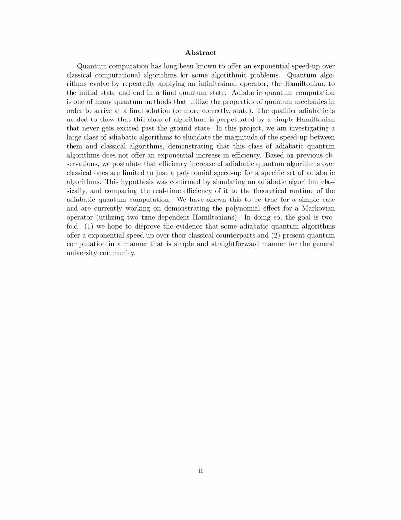
Figure 2.1 is a sample of single run of the simple case (Section 2.1) above. As can be seen in

the graph, the parameter s is smoothly varied over the defined range, and the smallest two

eigenvalues are shown by the green and the red lines. The blue line signifies the difference

between the two smallest eigenvalues, and the location of s at which the difference curve

reaches a minimum is the place where the ground state of the Hamiltonian (2.4) is found.

This run is aggregated with many others and spans over a range of qubits to attain a graph

such as is shown in Figure 2.2. Figure 2.2 shows a sample trial where each qubit (ranging

from 2 to 6) is run with a random input vector 10 times to produce an average value

These initial results are clearly promising, and a decreasing polynomial curve can be seen

from Figure 2.2. Although this was the limit of what we could run by this point due to time

11

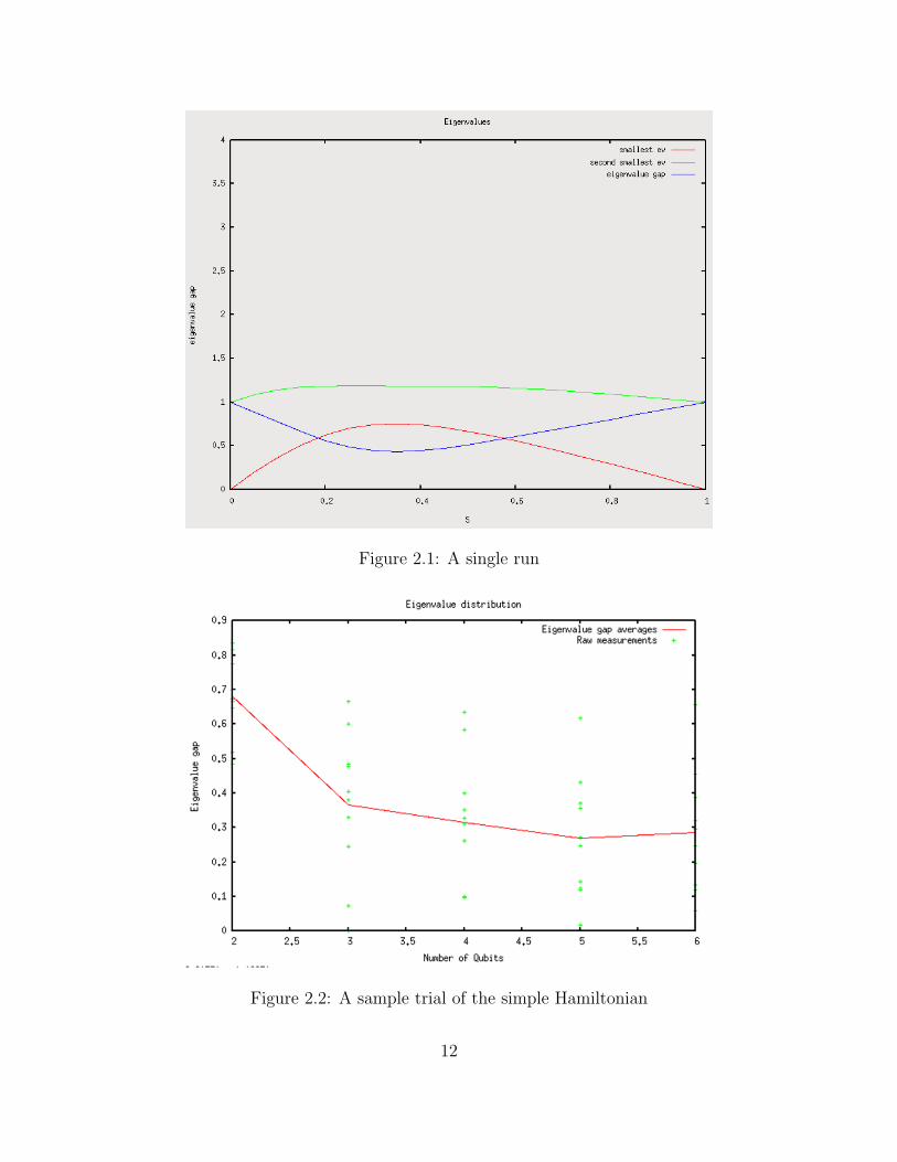
Figure 2.1: A single run

Figure 2.2: A sample trial of the simple Hamiltonian

12

constraints, we had also planned to simulate adiabatic efficiency with a more complicated

Hamiltonian constructed as a Markovian matrix as follows.

2.4 Simulation of an Example Adiabatic Algorithm

We considered a Markovian matrix as our Hamiltonian as a way to construct a simulated

annealing algorithm within the specifications of adiabatic quantum computation. For a

sanity check, we can ensure that Equation 2.5 is a stochastic matrix (in the L2-norm) since∑j(I + 1

nHi)ij = 0 and that exp [−β(Hf − fm)] has eigenvalues less than unity.

M(β) = I −(I +

1

nHi

)exp [−β(Hf − fm)] (2.5)

In Equation 2.5, β is used to signify T , which is bounded by the number of qubits selected

for the system n. We expect that very similar results to the above would have been observed.

13

Chapter 3

Conclusions and Future Work

These initial results indicate that as the number of qubits in the system increases, the eigen-

value gap of the ground state of the combined Hamiltonian H decreases polynomially. While

this supports the hypothesis described in Chapter 2 that adiabatic quantum computation

only offers a polynomial increase in efficiency over the exponential time reclaimed by stan-

dard quantum computation, this result is only preliminary.

We have brought up that this is simply a numerical simulation of several runs of the

Hamiltonian. Since we are trying to deal with all cases of the input wavefunction ψ and the

function fm = f(x) where x ∈ {0, 1}n, it would seem that a mathematical proof would yield

a more conclusive result for our hypothesis. Instead, we opted for a numerical simulation by

randomly feeding input wavefunctions and fm parameters to the computational Hamiltonian

as a mathematical proof would be infeasible.

3.1 Possible Effects to Adiabatic Quantum Computing

Since the preliminary conclusion here is that adiabatic quantum computation will only offer

a polynomial speedup over its classical counterpart as opposed to the exponential speedup

offered by standard quantum computation, this has serious ramifications about the potential

of creating an adiabatic quantum computer as the efficacy advantages have been decreased.

Adiabatic quantum computation, because of the local interaction restriction, seems to be

14

the most feasible avenue for creating a practical quantum computer [5, 1].

Several academic research groups and corporations have been working toward a feasible

representation of a quantum computer (as opposed to a classical simulation done here) that

exhibits all of the properties that a quantum computer should. The biggest challenges here

have been brought up – quantum decoherence stemming from the lack of separation of

the quantum system from the surrounding environment and the properties of the material

representing the qubits (trapped ion, topological, quantum dots, liquid NMR, Bose-Einstein

condensate) ensure that all features of the qubits stay intact. For example, IBM’s early

quantum computer built on NMR technology where the spins of atoms in a molecule can

be utilized as qubits [8] had issues with not exhibiting quantum entanglement (which they

acknowledged [9]).

An adiabatic quantum computer has the advantage of circumventing the problem of quan-

tum decoherence – as the quantum computer is always kept in the ground state throughout

the computation, the surrounding environment cannot force the lower-energy state that

would disrupt the computation. As long as the temperature of the environment is kept

below the ground state of the quantum computer, the qubits in the computation can be

kept coherent [1]. However, from the preliminary results here in this paper, it seems to give

up some of its efficiency gains by remaining in the ground state throughout the quantum

evolution.

One of the most notable attempts at building a quantum computer is D-Wave, a quantum

computing company based out of Burnaby, British Columbia that is attempting to build

an adiabatic quantum computer with 128 qubits using a superconductor approach. Their

approach has been poorly documented, and they claim that they have the most intellectual

property in the adiabatic quantum world “with over 75% of the patents.” It remains to be

seen whether an adiabatic quantum computer (along with standard quantum computers)

can be constructed and what their efficiency gains they bring to the computing world.

15

3.2 Ongoing and Future Work

Though much time was invested in discovering how quantum computers work and how

adiabatic quantum computers differ from their standard counterparts, additional time needs

to be spent to get results from the Markovian matrix and further trials need to be performed

(at least a couple thousand) in order to reach a solid result. Since we’re depending on a

numerical result of random inputs to arrive at an overall conclusion about adiabatic quantum

computation, many trials need to be done over many hundred hours in order to start using

these results as a basis for future work in the quantum computation field. We hope, however,

that through additional simulations we can arrive at a concrete conclusion and help to further

the area of adiabatic quantum computers.

3.3 Acknowledgements

Many thanks to Professor Dave Bacon (UW CSE) for his helpful guidance and immense

enthusiasm in converting my love of physical chemistry into quantum computation. Gregory

Crosswhite (UW Physics, grad student) has been invaluable in helping to debug code and

setting up the code environment for the quantum simulations. I would also like to thank

the Quantum Computing Theory Group for their engaging discussions and a willingness to

admit a quantum novice into their group.

A subset of this work was presented at Honors Research Symposium on May 8th, 2009,

and again to a broader audience at the University of Washington’s Undergraduate Research

Symposium on May 15th, 2009.

16

Bibliography

[1] E. Farhi, J. Goldstone, S. Gutmann, M. Sipser, Quantum Computation by Adiabatic

Evolution, arXiv: quant-ph/0001106v1

[2] E. Farhi, J. Goldstone, S. Gutmann, J. Lapan, A. Lundgren, Daniel Preda, A Quantum

Adiabatic Evolution Algorithm Applied to Random Instances of an NP-Complete Problem,

arXiv: quant-ph/0104129v1

[3] W. van Dam, M. Mosca, U. Vazirani, How Powerful is Adiabatic Quantum Computation,

arXiv: quant-ph/0206003v1

[4] E. Farhi, J. Goldstone, S. Gutmann, A Numerical Study of the Performance of a Quantum

Adiabatic Evolution Algorithm for Satisfiability, arXiv: quant-ph/0007071v1

[5] D. Aharonov, W. van Dam, J. Kempe, Z. Landau, S. Lloyd, O. Regev, Adiabatic

Quantum Computation is Equivalent to Standard Quantum Computation, arXiv: quant-

ph/0405098v2

[6] M. Nielsen, I. Chuang, Quantum Computation and Quantum Information. Cambridge

University Press, 2000.

[7] N.D. Mermin, Quantum Computer Science: An Introduction. Cambridge University

Press, 2007.

17

[8] L. Vandersypen et al. “Experimental realization of Shor’s quantum factoring algorithm

using nuclear magnetic resonance”, Nature 2001, 414, 883-887

[9] L. Vandersypen et al. “Separability of Very Noisy Mixed States and Implications for

NMR Quantum Computing”, Phys. Rev. Lett. 1999, 83, 1054-1057

18