The Log-Gamma Distribution and Non-Normal Error

Leigh J. Halliwell, FCAS, MAAA

ABSTRACT

Because insured losses are positive, loss distributions start from zero and are right-tailed. However,

residuals, or errors, are centered about a mean of zero and have both right and left tails. Seldom do error

terms from models of insured losses seem normal. Usually they are positively skewed, rather than

symmetric. And their right tails, as measured by their asymptotic failure rates, are heavier than that of the

normal. As an error distribution suited to actuarial modeling this paper presents and recommends the log-

gamma distribution and its linear combinations, especially the combination known as the generalized

logistic distribution. To serve as an example, a generalized logistic distribution is fitted by maximum

likelihood to the standardized residuals of a loss-triangle model. Much theory is required for, and

occasioned by, this presentation, most of which appears in three appendices along with some related

mathematical history.

Keywords: log-gamma, digamma, logistic, Euler-Mascheroni, cumulant, maximum likelihood, robust, bootstrap

1. Introduction

Since the late 1980s actuarial science has been moving gradually from methods to models. The movement

was made possible by personal computers; it was made necessary by insurance competition. Actuaries,

who used to be known for fitting curves and extrapolating from data, are now likely to be fitting models

and explaining data.

Statistical modeling seeks to explain a block of observed data as a function of known variables. The model

makes it possible to predict what will be observed from new instances of those variables. However, rarely,

if ever, does the function perfectly explain the data. A successful model, as well as seeming reasonable,

should explain the observations tolerably well. So the deterministic model Xy f gives way to the

approximation Xy f , which is restored to equality with the addition of a random error term:

ey Xf . The simplest model is the homoskedastic linear statistical model (LSM) with vector form

ey Xβ , in which 0eE and Iσ2eVar . According to LSM theory, yβ XXXˆ 1 - is the best

linear unbiased estimator (BLUE) of β, even if the elements of error vector e are not normally distributed.1

                                                            1 For explanations of the linear statistical model and BLUE see Judge [1988, §§5.5 and 5.7] and Halliwell [2015]. Although normality is not assumed in the model, it is required for the usual tests of significance, the t-test and the f-test. It would divert us here to argue whether randomness arises from reality or from our ignorance thereof. Between the world wars physicists Niels Bohr and Albert Einstein argued this at length – technically to a stalemate, although most physicists give the decision to Bohr. Either way, actuaries earn their keep by dealing with what the insurance industry legitimately perceives as randomness (“risk”). One reviewer commented, “From a Bayesian perspective, there is no real concept of randomness in the sense of an outcome that is not the result of a cause-effect relationship.”

This pushes conditional probability too far, to the tautology that abbXaX δProb . Information about some

variables from a group of jointly distributed random variables can affect the probability distribution of the others, as in the classic case of the positive-definite multivariate normal distribution. Such information tightens or narrows the “wave function,” without altogether collapsing it. The reviewer’s comment presumes the notion of Einstein’s hidden variables. Bayes is neither here nor there, for a variable that remains hidden forever, or ontologically, really is random. The truth intended by the comment is that modelers should not be lazy, that subject to practical constraints they should incorporate all relevant information into their models, even the so-called “collateral” information. Judge [1988, Chapter 7] devotes fifty pages to the Bayesian version of the LSM. Of course, whether randomness be ontological or epistemological, the goal of science is to mitigate it, if not to dispel it. This is especially the goal of actuarial science with regard to risk.

The fact that the errors resultant in most actuarial models are not normally distributed raises two questions.

First, does non-normality in the randomness affect the accuracy of a model’s predictions? The answer is

“Yes, sometimes seriously.” Second, can models be made “robust,”2 i.e., able to deal properly with non-

normal error? Again, “Yes.” Three attempts to do so are 1} to relax parts of BLUE, especially linearity

and unbiasedness (robust estimation), 2} to incorporate explicit distributions into models (GLM), and 3} to

bootstrap.3 Bootstrapping a linear model begins with solving it conventionally. One obtains β̂ and the

expected observation vector βy ˆXˆ . Gleaning information from the residual vector yye ˆˆ , one can

simulate proper, or more realistic, “pseudo-error” vectors *ie and pseudo-observations *ˆ ii eyy .

Iterating the model over the iy will produce pseudo-estimates iβ̂ and pseudo-predictions in keeping with

the apparent distribution of error. Of the three attempts, bootstrapping is the most commonsensical.

Our purpose herein is to introduce a distribution for non-normal error that is suited to bootstrapping in

general, but especially as regards the asymmetric and skewed data that actuaries regularly need to model.

As useful candidates for non-normal error, Sections 2 and 3 will introduce the log-gamma random variable

and its linear combinations. Section 4 will settle on a linear combination that arguably maximizes the ratio

of versatility to complexity, the generalized logistic random variable. Section 5 will examine its special

cases. Finally, Section 6 will estimate by maximum likelihood the parameters of one such distribution from

actual data. The most mathematical and theoretical subjects are relegated to Appendices A-C.

                                                            2 “Models that perform well even when the population does not conform precisely to the parametric family are said to be robust” (Klugman [1998, §2.4.3]). “A robust estimator … produces estimates that are ‘good’ (in some sense) under a wide variety of possible data-generating processes” (Judge [1988, Introduction to Chapter 22]). Chapter 22 of Judge contains thirty pages on robust estimation. 3 For descriptions of bootstrapping see Klugman [1998, Example 2.19 in §2.4.3] and Judge [1988, Chapter 9, §9.A.1]. However, they both describe bootstrapping, or resampling, from the empirical distribution of residuals. Especially when observations are few (as in the case of our example in Section 6 with eighty-five observations) might the modeler want to bootstrap/resample from a parametric error distribution. Not to give away “free cover” would require bootstrapping from a parametric distribution, unless predictive errors were felt to be well represented by the residuals. A recent CAS monograph that combines GLM and bootstrapping is Shapland [2016].

2. The Log-Gamma Random Variable

If θα,~ GammaX , then XY ln is a random variable whose support is the entire real line.4 Hence,

the logarithm converts a one-tailed distribution into a two-tailed. Although a leftward shift of X would

move probability onto the negative real line, such a left tail would be finite. The logarithm is a natural way,

even the natural way, to transform one infinite tail into two infinite tails.5 Because the logarithm function

strictly increases, the probability density function of θα,~ Gamma-LogY is:6

α

θ

1α

θ

θα

1

θ

1

θα

1

ueu

ueuu

eXY

eee

ee

du

deefuf

uu

Y

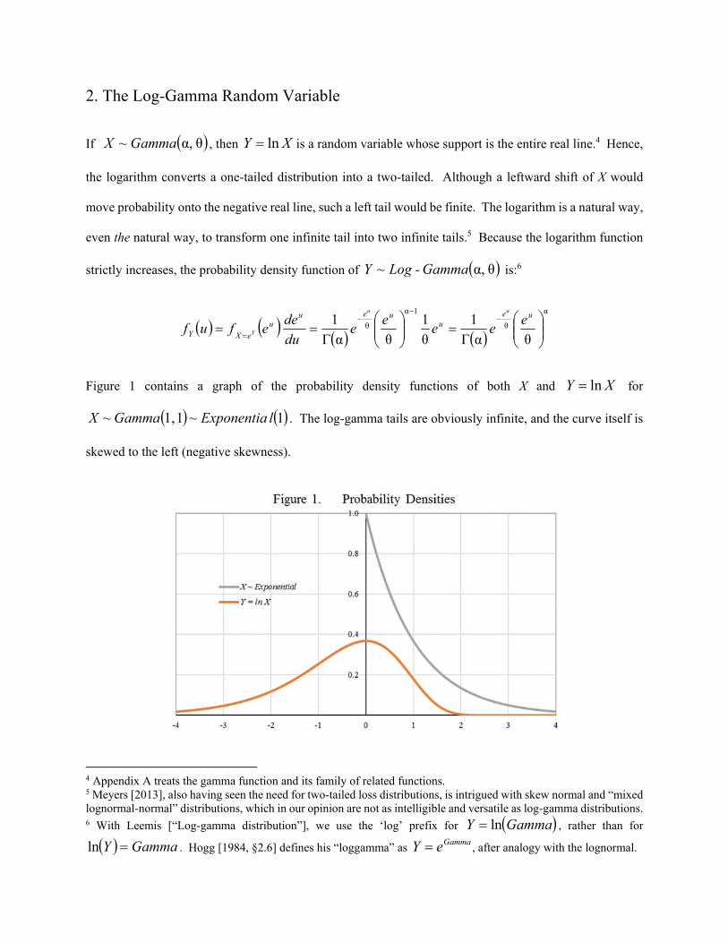
Figure 1 contains a graph of the probability density functions of both X and XY ln for

1~11,~ lExponentiaGammaX . The log-gamma tails are obviously infinite, and the curve itself is

skewed to the left (negative skewness).

                                                            4 Appendix A treats the gamma function and its family of related functions. 5 Meyers [2013], also having seen the need for two-tailed loss distributions, is intrigued with skew normal and “mixed lognormal-normal” distributions, which in our opinion are not as intelligible and versatile as log-gamma distributions. 6 With Leemis [“Log-gamma distribution”], we use the ‘log’ prefix for GammaY ln , rather than for

GammaY ln . Hogg [1984, §2.6] defines his “loggamma” as GammaeY , after analogy with the lognormal.

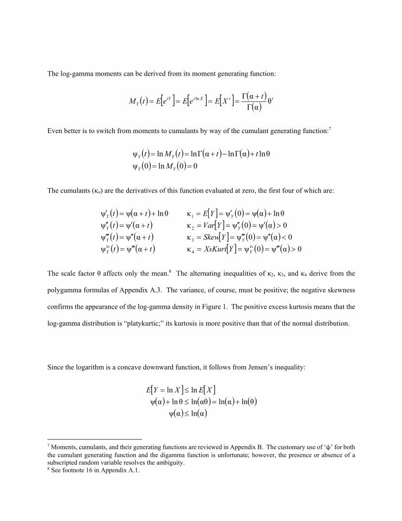
The log-gamma moments can be derived from its moment generating function:

ttXttYY

tXEeEeEtM θ

α

αln

Even better is to switch from moments to cumulants by way of the cumulant generating function:7

00ln0ψ

θlnαlnαlnlnψ

YY

YY

M

tttMt

The cumulants (κn) are the derivatives of this function evaluated at zero, the first four of which are:

0αψ0ψκαψψ

0αψ0ψκαψψ

0αψ0ψκαψψ

θlnαψ0ψκθlnαψψ

iv4

iv3

2

1

YY

YY

YY

YY

YXsKurttt

YSkewtt

YVartt

YEtt

The scale factor θ affects only the mean.8 The alternating inequalities of κ2, κ3, and κ4 derive from the

polygamma formulas of Appendix A.3. The variance, of course, must be positive; the negative skewness

confirms the appearance of the log-gamma density in Figure 1. The positive excess kurtosis means that the

log-gamma distribution is “platykurtic;” its kurtosis is more positive than that of the normal distribution.

Since the logarithm is a concave downward function, it follows from Jensen’s inequality:

αlnαψ

θlnαlnαθlnθlnαψ

lnln

XEXYE

                                                            7 Moments, cumulants, and their generating functions are reviewed in Appendix B. The customary use of ‘ψ’ for both the cumulant generating function and the digamma function is unfortunate; however, the presence or absence of a subscripted random variable resolves the ambiguity. 8 See footnote 16 in Appendix A.1.

Because the probability is not amassed, the inequality is strict: αlnαψ for α > 0. However, when

αθXE is fixed at unity and as α , the variance of X approaches zero. Hence,

01lnαψαln limα

. It is not difficult to prove that

αψαln lim0α

, as well as that

αψαln strictly decreases. Therefore, for every y > 0 there exists exactly one α > 0 for which

αψαln y .

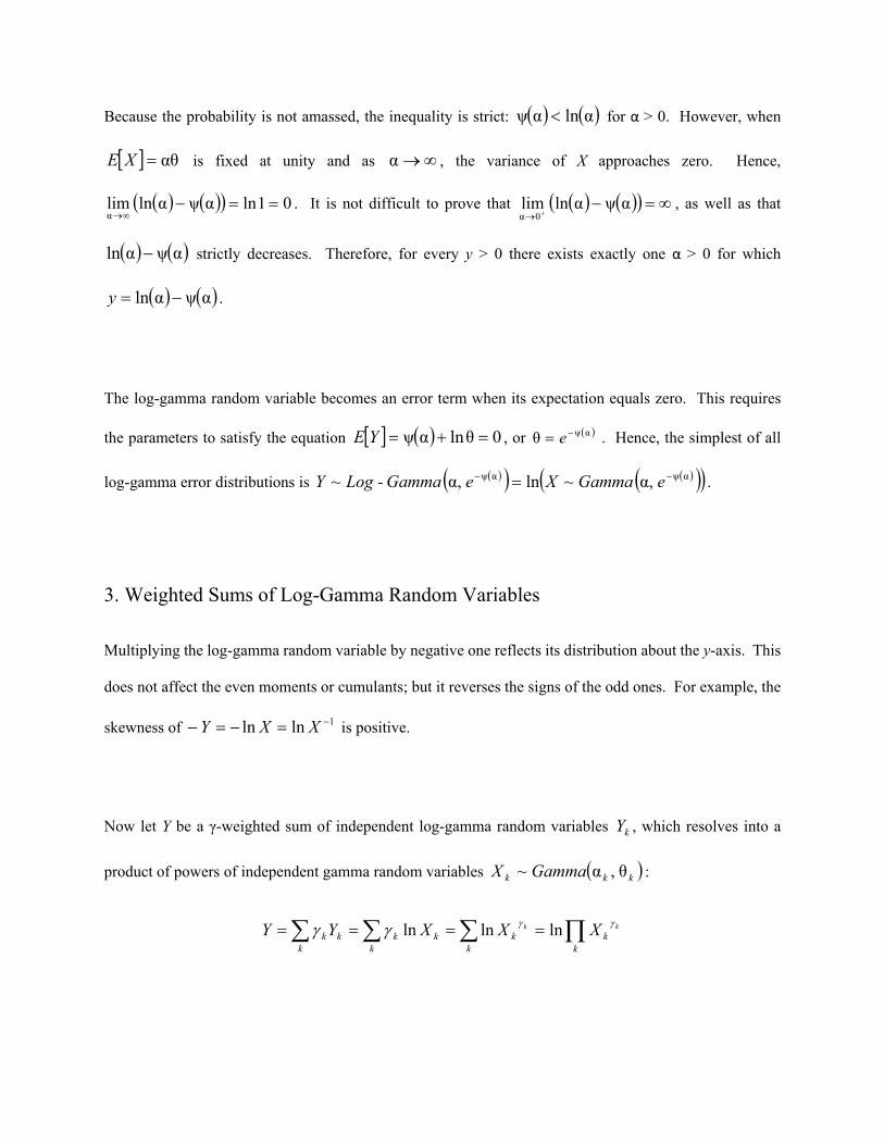
The log-gamma random variable becomes an error term when its expectation equals zero. This requires

the parameters to satisfy the equation 0θlnαψ YE , or αψθ e . Hence, the simplest of all

log-gamma error distributions is αψαψ α,lnα,~ eGamma~XeGamma-LogY .

3. Weighted Sums of Log-Gamma Random Variables

Multiplying the log-gamma random variable by negative one reflects its distribution about the y-axis. This

does not affect the even moments or cumulants; but it reverses the signs of the odd ones. For example, the

skewness of 1lnln XXY is positive.

Now let Y be a γ-weighted sum of independent log-gamma random variables kY , which resolves into a

product of powers of independent gamma random variables kkk GammaX θ,α~ :

k

kk

kk

kkk

kkkk XXXYY lnlnln

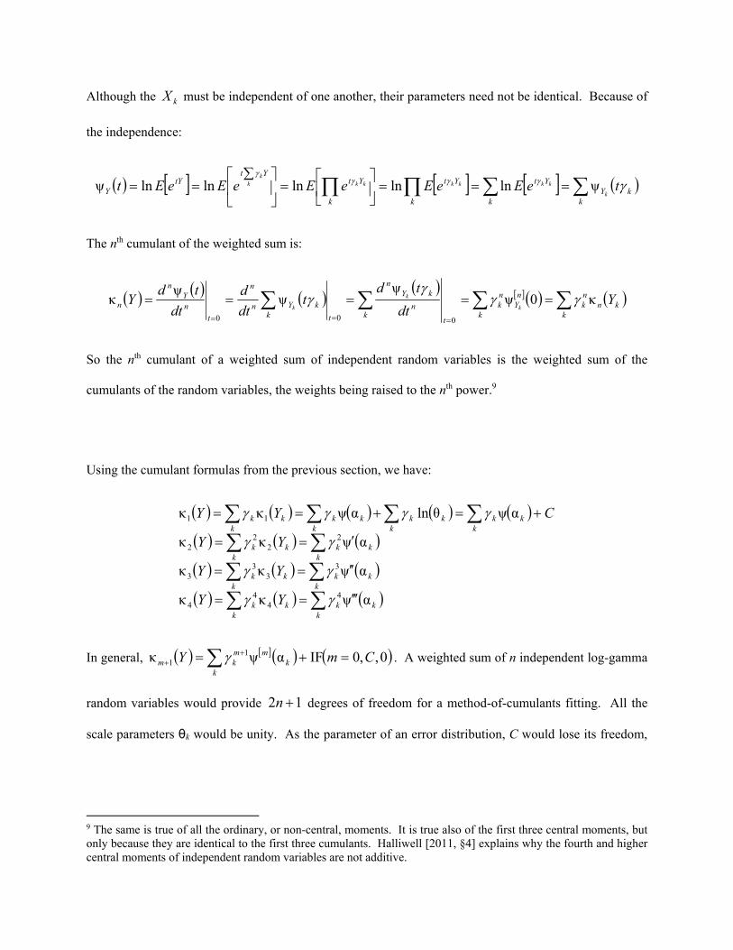
Although the kX must be independent of one another, their parameters need not be identical. Because of

the independence:

kkY

k

Yt

k

Yt

k

YtYt

tYY teEeEeEeEeEt

k

kkkkkkkk

ψlnlnlnlnlnψ

The nth cumulant of the weighted sum is:

k

knnk

k

nY

nk

tk

n

kYn

tkkYn

n

t

nY

n

n Ydt

tdt

dt

d

dt

tdY

k

k

kκ0ψ

ψψ

ψκ

000

So the nth cumulant of a weighted sum of independent random variables is the weighted sum of the

cumulants of the random variables, the weights being raised to the nth power.9

Using the cumulant formulas from the previous section, we have:

kkk

kkk

kkk

kkk

kkk

kkk

kkk

kkk

kkk

kkk

YY

YY

YY

CYY

αψκκ

αψκκ

αψκκ

αψθlnαψκκ

44

44

33

33

22

22

11

In general, 0,,0IFαψκ 11 CmY

kk

mmkm

. A weighted sum of n independent log-gamma

random variables would provide 12 n degrees of freedom for a method-of-cumulants fitting. All the

scale parameters θk would be unity. As the parameter of an error distribution, C would lose its freedom,

                                                            9 The same is true of all the ordinary, or non-central, moments. It is true also of the first three central moments, but only because they are identical to the first three cumulants. Halliwell [2011, §4] explains why the fourth and higher central moments of independent random variables are not additive.

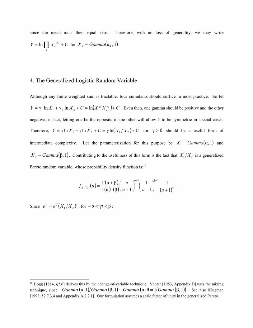
since the mean must then equal zero. Therefore, with no loss of generality, we may write

CXYk

kk ln for 1,α~ kk GammaX .

4. The Generalized Logistic Random Variable

Although any finite weighted sum is tractable, four cumulants should suffice in most practice. So let

CXXCXXY 21 γ2

γ12211 lnlnγlnγ . Even then, one gamma should be positive and the other

negative; in fact, letting one be the opposite of the other will allow Y to be symmetric in special cases.

Therefore, CXXCXXY 2121 lnγlnγlnγ for 0γ should be a useful form of

intermediate complexity. Let the parameterization for this purpose be 1α,~1 GammaX and

1β,~2 GammaX . Contributing to the usefulness of this form is the fact that 21 XX is a generalized

Pareto random variable, whose probability density function is:10

2

1β1α

1

1

1

1

1βα

βα21

uuu

uuf XX

Since γ21 XXee CY , for βγα t :

                                                            10 Hogg [1884, §2.6] derives this by the change-of-variable technique. Venter [1983, Appendix D] uses the mixing

technique, since 1β,1θα,~1β,1α, GammaGammaGammaGamma . See also Klugman

[1998, §2.7.3.4 and Appendix A.2.2.1]. Our formulation assumes a scale factor of unity in the generalized Pareto.

βα

γβγα

11

1

1γβγα

βα

βα

γβγα

11

1

1βα

βα

02

1γβ1γα

02

1β1αγ

γ21

tte

u

du

uu

u

tt

tte

u

du

uu

uue

XXEeeEtM

Ct

u

ttCt

u

tCt

tCttYY

Hence, the cumulant generating function and its derivatives are:

ttt

ttt

ttt

Cttt

ttCttMt

Y

Y

Y

Y

YY

γβψγαψγψ

γβψγαψγψ

γβψγαψγψ

γβψγαψγψ

βlnγβlnαlnγαlnlnψ

4iv

3

2

And so, the cumulants are:

0βψαψγ0ψκ

βψαψγ0ψκ

0βψαψγ0ψκ

βψαψγ0ψκ

4iv4

33

22

1

Y

Y

Y

Y

YXsKurt

YSkew

YVar

CYE

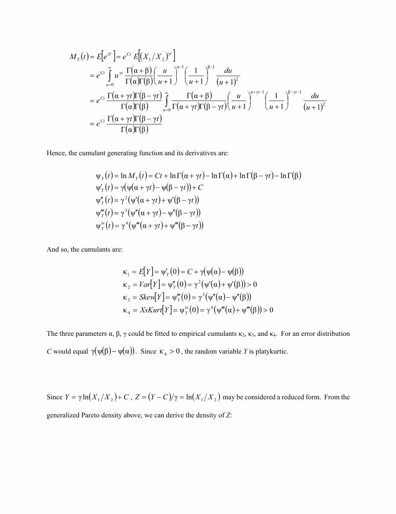
The three parameters α, β, γ could be fitted to empirical cumulants κ2, κ3, and κ4. For an error distribution

C would equal αψβψγ . Since 0κ 4 , the random variable Y is platykurtic.

Since CXXY 21lnγ , 21lnγ XXCYZ may be considered a reduced form. From the

generalized Pareto density above, we can derive the density of Z:

βα

2

1β1α

1

1

1βα

βα

1

1

1

1

1βα

βα

21

uu

u

u

uuu

u

uu

eXXZ

ee

e

eeee

e

du

deefuf Z

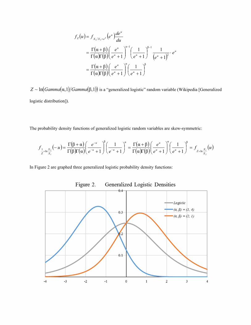
1,β1,αln~ GammaGammaZ is a “generalized logistic” random variable (Wikipedia [Generalized

logistic distribution]).

The probability density functions of generalized logistic random variables are skew-symmetric:

uf

ee

e

ee

euf

X

XZuu

u

uu

u

X

X

Z 2

1

1

2 ln

βααβ

ln1 1

1

1βα

βα

1

1

1αβ

αβ

In Figure 2 are graphed three generalized logistic probability density functions:

The density is symmetric if and only if βα ; the gray curve is that of the logistic density, for which

1βα . The mode of the generalized-logistic β,α density is βαlnmode u . Therefore, the mode

is positive [or negative] if and only if βα [or βα ]. Since the digamma and tetragamma functions

ψψ, strictly increase over the positive reals, the signs of βψαψ ZE and

βψαψ ZSkew are the same as the sign of βα . The positive mode of the orange curve (2, 1)

implies positive mean and skewness, whereas for the blue curve (1, 4) they are negative.

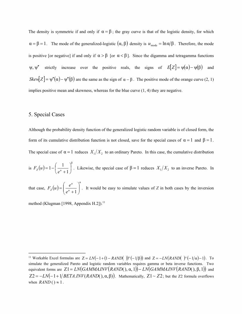
5. Special Cases

Although the probability density function of the generalized logistic random variable is of closed form, the

form of its cumulative distribution function is not closed, save for the special cases of 1α and 1β .

The special case of 1α reduces 21 XX to an ordinary Pareto. In this case, the cumulative distribution

is β

1

11

uZ euF . Likewise, the special case of 1β reduces 21 XX to an inverse Pareto. In

that case, α

1

u

u

Z e

euF . It would be easy to simulate values of Z in both cases by the inversion

method (Klugman [1998, Appendix H.2]).11

                                                            11 Workable Excel formulas are β1^11Z RANDLN and 1α1^Z RANDLN . To

simulate the generalized Pareto and logistic random variables requires gamma or beta inverse functions. Two

equivalent forms are 1,β),(.1,α),(.Z1 RANDINVGAMMALNRANDINVGAMMALN and

β) α, ),((11Z2 RANDBETA.INVLN . Mathematically, 2~Z1 Z ; but the Z2 formula overflows

when 1)( RAND .

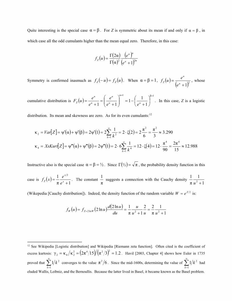
Quite interesting is the special case βα . For Z is symmetric about its mean if and only if βα , in

which case all the odd cumulants higher than the mean equal zero. Therefore, in this case:

2α

α

21α

2α

u

u

Ze

euf

Symmetry is confirmed inasmuch as ufuf ZZ . When 1βα , 21

u

u

Ze

euf , whose

cumulative distribution is 1β1α

1

11

11

uu

u

u

u

Z ee

e

e

euF . In this case, Z is a logistic

distribution. Its mean and skewness are zero. As for its even cumulants:12

988.1215

2π

90

π124ζ12

1621ψ2βψαψκ

290.33

π

6

π22ζ2

121ψ2βψαψκ

44

144

22

122

k

k

kZXsKurt

kZVar

Instructive also is the special case ½βα . Since π½ , the probability density function in this

case is 1π

1 2

x

x

Z e

exf . The constant

π

1 suggests a connection with the Cauchy density

1

1

π

12 u

(Wikepedia [Cauchy distribution]). Indeed, the density function of the random variable 2ZeW is:

1

1

π

22

1π

1ln2ln2

22ln2

uuu

u

du

udufuf WZW

                                                            12 See Wikipedia [Logistic distribution] and Wikipedia [Riemann zeta function]. Often cited is the coefficient of

excess kurtosis: 2.13π152πκκγ2242

242 . Havil [2003, Chapter 4] shows how Euler in 1735

proved that

1

21k

k converges to the value 6π 2 . Since the mid-1600s, determining the value of

1

21k

k had

eluded Wallis, Leibniz, and the Bernoullis. Because the latter lived in Basel, it became known as the Basel problem.

This is the density function of the absolute value of the standard Cauchy random variable.13

6. A Maximum-Likelihood Example

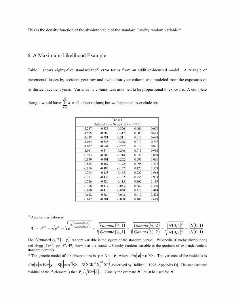
Table 1 shows eighty-five standardized14 error terms from an additive-incurred model. A triangle of

incremental losses by accident-year row and evaluation-year column was modeled from the exposures of

its thirteen accident years. Variance by column was assumed to be proportional to exposure. A complete

triangle would have 9113

1

k

k observations; but we happened to exclude six.

                                                            13 Another derivation is:

10,

10,

10,

10,

2½,

2½,

1½,

1½,2

21½,

1½,ln

2

N

N

N

N

Gamma

Gamma

Gamma

GammaeeeW Gamma

Gamma

ZZ

The 21χ~2½,Gamma random variable is the square of the standard normal. Wikipedia [Cauchy distribution]

and Hogg [1984, pp. 47, 49] show that the standard Cauchy random variable is the quotient of two independent standard normals. 14 The generic model of the observations is ey Xβ , where 2σeVar . The variance of the residuals is

XXXXσˆXˆ1-12 βye VarVar , as derived by Halliwell [1996, Appendix D]. The standardized

residual of the ith element is then iii Var ee ˆˆ . Usually the estimate 2σ̂ must be used for 2σ .

Table 1Ordered Error Sample (85 = 17 × 5)

-2.287 -0.585 -0.326 -0.009 0.658-1.575 -0.582 -0.317 0.009 0.663-1.428 -0.581 -0.311 0.010 0.698-1.034 -0.545 -0.298 0.012 0.707-1.022 -0.544 -0.267 0.017 0.821-1.011 -0.514 -0.260 0.019 0.998-0.913 -0.503 -0.214 0.038 1.009-0.879 -0.501 -0.202 0.090 1.061-0.875 -0.487 -0.172 0.095 1.227-0.856 -0.486 -0.167 0.123 1.559-0.794 -0.453 -0.165 0.222 1.966-0.771 -0.435 -0.162 0.255 1.973-0.726 -0.429 -0.115 0.362 2.119-0.708 -0.417 -0.053 0.367 2.390-0.670 -0.410 -0.050 0.417 2.414-0.622 -0.384 -0.042 0.417 2.422-0.612 -0.381 -0.038 0.488 2.618

The sample mean is nearly zero at 0.001. Three of the five columns are negative, and the positive errors

are more dispersed than the negative. Therefore, this sample is positively skewed, or skewed to the right.

Other sample cumulants are 0.850 (variance), 1.029 (skewness), and 1.444 (excess kurtosis). The

coefficients of skewness and of kurtosis are 1.314 and 1.999.

By maximum likelihood we wished to explain the sample as coming from CZY γ , where

1,β1,αln~ln 21 GammaGammaXXZ , the generalized logistic variable of Section 4 with

distribution:

βα

1

1

1βα

βα

uu

u

Z ee

euf

So, defining γγ,; CuCuz , whereby ZYz , we have the distribution of Y:

γ

1

1

1

1βα

βαβα

uzuz

uz

YzZY ee

euzuzfuf

The logarithm, or the log-likelihood, is:

γln1lnβααβlnαlnβαlnln uzY euzuf

This is a function in four parameters; C and γ are implicit in uz . With all four parameters free, the

likelihood of the sample could be maximized. Yet it is both reasonable and economical to estimate Y as a

“standard-error” distribution, i.e., as having zero mean and unit variance. In Excel it sufficed us to let the

Solver add-in maximize the log-likelihood with respect to α and β, giving due consideration that C and γ,

constrained by zero mean and unit variance, are themselves functions of α and β. As derived in Section 4,

βψαψγ CYE and βψαψγ 2 YVar . Hence, standardization requires that

βψαψ1βα,γ and that αψβψβα,γβα, C .  The log-likelihood maximized at

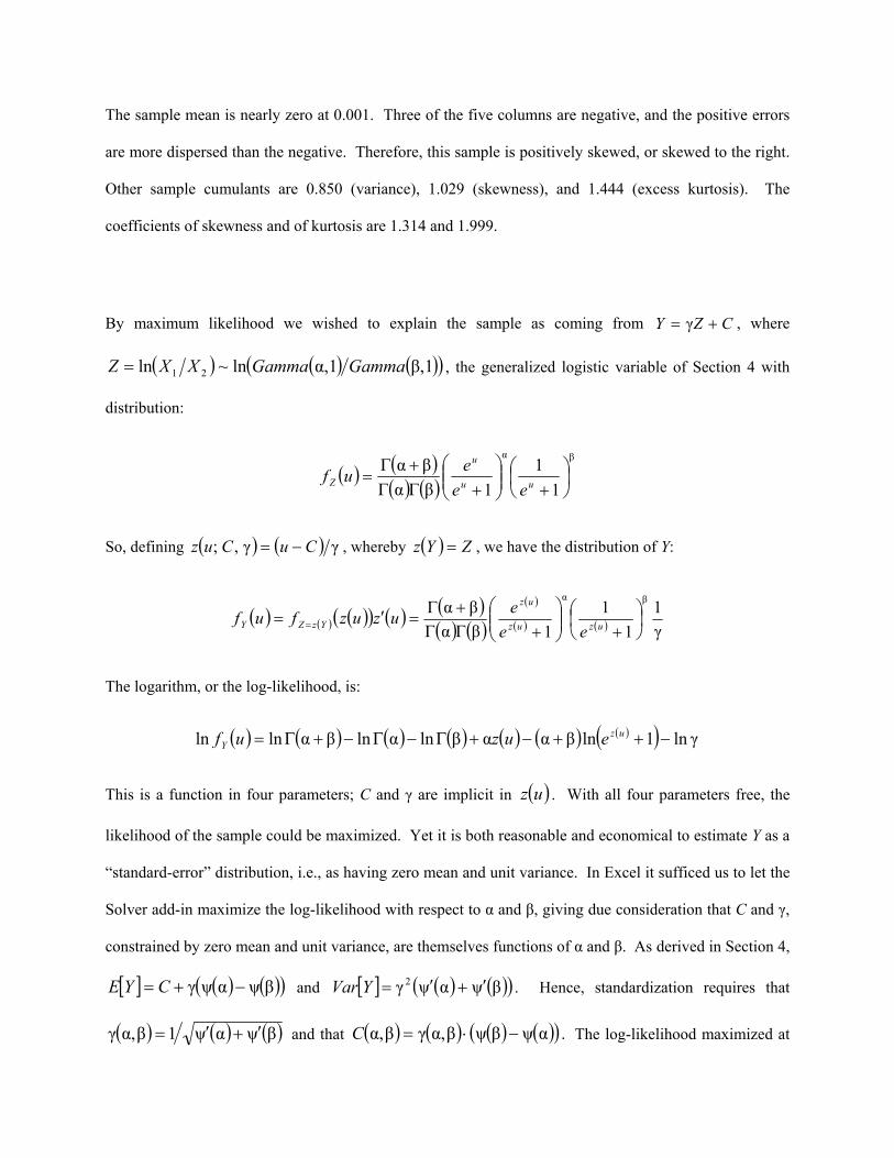
0.326ˆ α and 0.135ˆ β . Numerical derivatives of the GAMMALN function approximated the

digamma and trigamma functions at these values. The remaining parameters for a standardized distribution

must be 561.0ˆ C and 122.0ˆ γ . Figure 3 graphs the maximum-likelihood result:

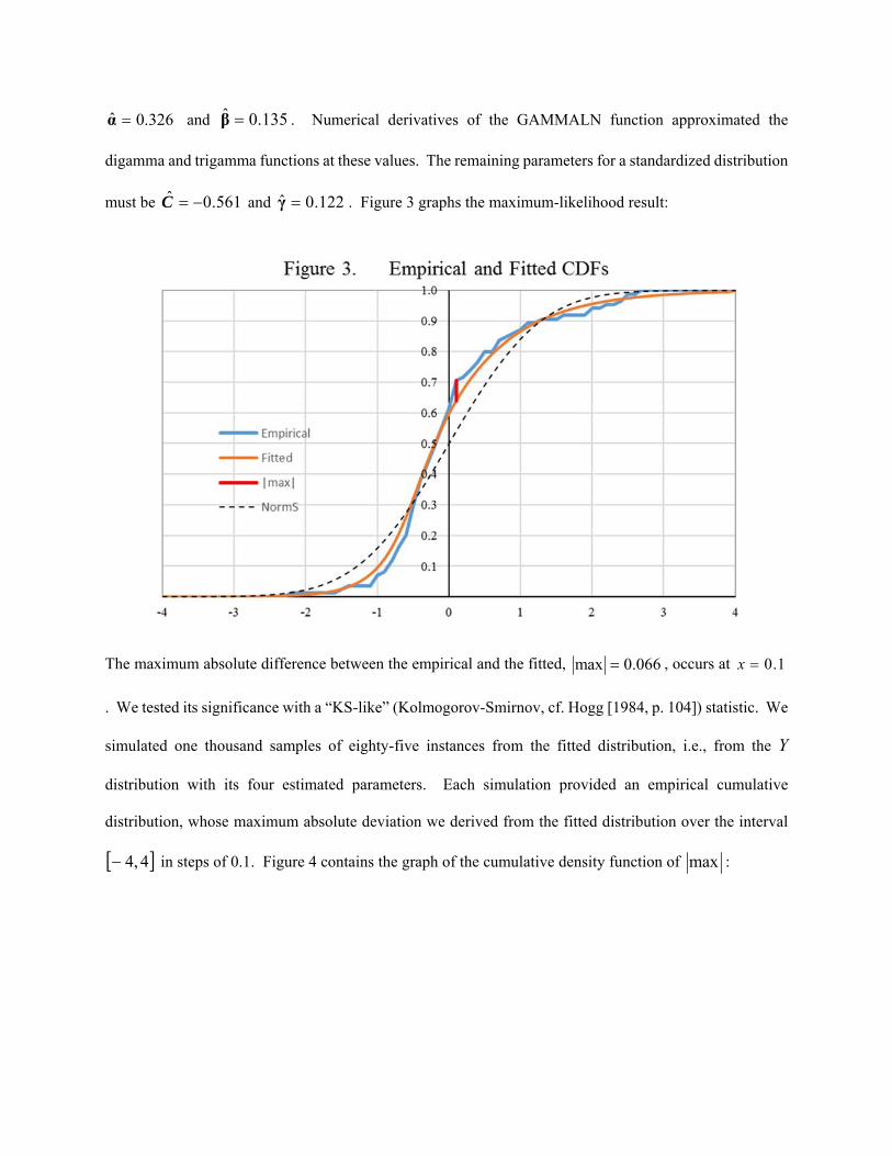
The maximum absolute difference between the empirical and the fitted, 066.0max , occurs at 1.0x

. We tested its significance with a “KS-like” (Kolmogorov-Smirnov, cf. Hogg [1984, p. 104]) statistic. We

simulated one thousand samples of eighty-five instances from the fitted distribution, i.e., from the Y

distribution with its four estimated parameters. Each simulation provided an empirical cumulative

distribution, whose maximum absolute deviation we derived from the fitted distribution over the interval

4,4 in steps of 0.1. Figure 4 contains the graph of the cumulative density function of max :

The actual deviation of 0.066 coincides with the thirty-first percentile, or about with the lower tercile. The

dashed line in Figure 3 (legend “NormS”) represents the cumulative standard-normal distribution. The

empirical distribution has more probability below zero and a heavier right tail. Simulations with these

logistic error terms are bound to be more accurate than simulations defaulted to normal errors.15

8. Conclusion

Actuaries are well schooled in loss distributions, which are non-negative, positively skewed, and right-

tailed. The key to a versatile distribution of error is to combine logarithms of loss distributions. Because

most loss distributions are transformations of the gamma distribution, the log-gamma distribution covers

most of the possible combinations. The generalized logistic distribution strikes a balance between

versatility and complexity. It should be a recourse to the actuary seeking to bootstrap a model whose

residuals are not normally distributed.

                                                            15 Taking trigamma and tetragamma values from www.easycalculation.com/statistics/polygamma-function.php, we

calculated the higher cumulants: 496.1κ3 YSkew and 180.4κ 4 YXsKurt . Since Y is

standardized, these values double as coefficients of skewness and kurtosis. That they, especially the kurtosis, are greater than the empirical coefficients, 1.314 and 1.999, is evidence for the inferiority of the method of moments.

References

Artin, Emil, The Gamma Function, New York, Dover, 2015 (ET “Einführung in die Theorie der Gammafunktion,” Hamburger Mathematische Einzelshriften, 1931).

Daykin, Chris D., T. Pentikäinen, and M. Pesonen, Practical Risk Theory for Actuaries, London: Chapman & Hall, 1994.

Halliwell, Leigh J., “Loss Prediction by Generalized Least Squares,” Proceedings of the Casualty Actuarial Society, LXXXIII (1996), 156-193, www.casact.org/pubs/proceed/proceed96/96436.pdf.

Halliwell, Leigh J., “Conditional Probability and the Collective Risk Model,” Casualty Actuarial Society E-Forum, Spring 2011, www.casact.org/pubs/forum/11spforum/Halliwell.pdf.

Halliwell, Leigh J., “The Gauss-Markov Theorem: Beyond the BLUE,” Casualty Actuarial Society E-Forum, Fall 2015, www.casact.org/pubs/forum/15fforum/Halliwell_GM.pdf.

Havil, Julian, Gamma: Exploring Euler’s Constant, Princeton University Press, 2003.

Hogg, Robert V., and S. A. Klugman, Loss Distributions, New York, Wiley, 1984.

Judge, George G., R. C. Hill, W. E. Griffiths, H. Lütkepohl, and T. Lee, Introduction to the Theory and Practice of Econometrics, 2nd ed., New York: Wiley, 1988.

Klugman, Stuart A., H. H. Panjer, and G. E. Wilmot, Loss Models: From Data to Decisions, New York: Wiley, 1998.

Leemis, Larry, “Log-gamma distribution,” www.math.wm.edu/~leemis/chart/UDR/PDFs/Loggamma.pdf.

Meyers, Glenn, “The Skew Normal Distribution and Beyond,” Actuarial Review, May 2013, p. 15, www.casact.org/newsletter/pdfUpload/ar/AR_May2013_1.pdf.

Shapland, Mark R., Using the ODP Bootstrap Model: A Practitioner’s Guide, CAS Monograph Series Number 4, Casualty Actuarial Society (2016), www.casact.org/pubs/monographs/papers/04-shapland.pdf.

Venter, Gary G., “Transformed Beta and Gamma Distributions and Aggregate Losses,” Proceedings of the Casualty Actuarial Society, LXX (1983), 156-193, www.casact.org/pubs/proceed/proceed83/83156.pdf.

Wikipedia contributors, Wikipedia, The Free Encyclopedia, (accessed March 2017):

“Bohr–Mollerup theorem,” https://en.wikipedia.org/wiki/Bohr–Mollerup_theorem

“Cauchy distribution,” https://en.wikipedia.org/wiki/Cauchy_distribution

“Gamma function,” https://en.wikipedia.org/wiki/Gamma_function

“Generalized logistic distribution,” https://en.wikipedia.org/wiki/Generalized_logistic_distribution

“Logistic distribution,” https://en.wikipedia.org/wiki/Logistic_distribution

“Polygamma function,” https://en.wikipedia.org/wiki/Polygamma_function

“Riemann zeta function,” https://en.wikipedia.org/wiki/Riemann_zeta_function

Appendix A

The Gamma, Log-Gamma, and Polygamma Functions

A.1. The Gamma Function as an Integral

The modern form of the gamma function is

0

1ααx

x dxxe . The change of variable xet (or

ttx 1lnln ) transforms it into:

1

0

1α0

1

1α1

ln1

lnαtt

dttt

dt

tt

According to Havil [2003, p. 53], Leonhard Euler used the latter form in his pioneering work during 1729-

1730. It was not until 1809 that Legendre named it the gamma function and denoted it with the letter ‘Γ’.

The function records the struggle between the exponential function xe and the power function 1αx , in

which the former ultimately prevails and forces the convergence of the integral for α > 0.

Of course, 110

x

xdxe . The well-known recurrence formula αα1α follows from

integration by parts:

1α0ααα0

11α

0

α

0

α

0

α

0

1α

x

x

x

xx

x

x

x

x dxxeedxxexdedxxe

It is well to note that in order for

0

αxe x to equal zero, α must be positive. For positive-integral values of

α, !1αα ; so the gamma function extends the factorial to the positive real numbers. In this domain

the function is continuous, even differentiable, as well as positive. Although

αlim0α

,

111αlimααlim0α0α

. So α

1~α as 0α . As α increases away from zero, the

function decreases to a minimum of approximately 886.0462.1 , beyond which it increases. So, over

the positive real numbers the gamma function is ‘U’ shaped, or concave upward.

The simple algebra

0

1α0

1α

α

1

αα

α1

x

xx

x

dxxe

dxxe

indicates that 1α

α

1

xexf x is

the probability density function of what we will call a Gamma(α, 1)-distributed random variable, or simply

Gamma(α)-distributed with 1θ understood.16 For αk , the kth moment of X ~ Gamma(α) is:

α

α

α

1

α

α

α

1

0

1α

0

1α

kdxxe

k

kdxxexXE

x

kx

x

xkk

Therefore, for k = 1 and 2, αXE and 1αα2 XE . Hence, αXVar .

                                                            16 Similarly, Venter [1983, p. 157]: “The percentage of this integral reached by integrating up to some point x defines a probability distribution, i.e., the probability of being less than or equal to x.” The multiplication of this random

variable by a scale factor θ > 0 is Gamma(α, θ)-distributed with density θ

1

θα

11α

θθα,

xexf

x

Gamma , as

found under equivalent forms in Hogg [1984, p. 226] and Klugman [1998, Appendix A.3.2.1]. Because this paper deals with logarithms of gamma random variables, in which products turn into sums, we will often ignore scale factors.

A.2. The Gamma Function as an Infinite Product

Euler found that the gamma function could be expressed as the infinite product:

n

xxx

n

xnxx

nnx

x

n

x

n1

11

lim1

!lim

As a check, 11

lim!1

!lim1

n

n

n

nnnn

. Moreover, the recurrence formula is satisfied:

xxxn

n

xnxx

nnx

xnxnx

nnx

n

x

n

x

n

1lim

1

!lim

11

!lim1

1

Hence, by induction, the integral and infinite-product definitions are equivalent for positive-integral values

of x. It is the purpose of this section to extend the equivalence to all positive real numbers.

The proof is easier in logarithms. The log-gamma function is

0

1αlnαlnx

x dxxe . The form of its

recursive formula is αlnαlnααln1αln . Its first derivative is:

YEdxxxe

dxxxe

d

d

x

xx

x

0

1α0

1α

lnα

1

α

ln

α

ααln

ααln

So the first derivative of αln is the expectation of α~ Gamma-LogY , as defined in Section 2.

The second derivative is:

0

lnα

1

α

α

α

α

αα

αααα

α

α

ααln

22

2

0

21α

2

YVarYEYE

YEdxxxe

d

d

x

x

Because the second derivative is positive, the log-gamma function is concave upward over the positive real

numbers.

Now let ,3,2n and 1,0x . So 110 nxnnn . We consider the slope of the

log-gamma secants over the intervals nn ,1 , xnn , , and 1, nn . Due to the upward concavity,

the order of these slopes must be:

nn

nn

nxn

nxn

nn

nn

1

ln1lnlnln

1

1lnln

Using the recurrence formula and multiplying by positive x, we continue:

nnxxnnnx

nxnxnnx

lnlnlnln1ln

lnlnln1ln

But

1

1

lnlnn

k

kn and

1

1

lnlnlnlnn

k

xkxxxn . Hence:

1

1

1

1

1

1

1

1

1

1

1

1

1

1

1

1

1

1

1lnlnlnln1lnln1ln

lnlnlnlnlnlnlnln1ln

lnlnlnlnlnln1ln

n

k

n

k

n

k

n

k

n

k

n

k

n

k

n

k

n

k

k

xxnxx

k

xxnx

xkxknxxxkxknx

knxxkxxknx

This string of inequalities, in the middle of which is xln , is true for ,3,2n . As n approaches

infinity, 01ln1

limln1

lnlim1lnlnlim

x

n

nx

n

nxnxnx

nnn. So xln is

sandwiched between two series that have the same limit. Hence:

n

kn

n

kn

k

xnxx

k

xnxxx

1

1

1

1lnlnlimln

1ln1lnlimlnln

 

If the limit did not converge, then xln would not converge. Nevertheless, Appendix C constructs a

proof of the limit’s convergence. But for now we can finish this section by exponentiation:

n

xxx

n

k

xn

x

ex

ex

ex

x

n

n

k

x

n

k

xnx

n

k

xnx

x

n

k

n

kn

11

1lim

1lim

1

lim1

1

1

1lnln

1lnlnlim

ln

1

1

The infinite-product form converges for all complex numbers ,2,1,0 z ; it provides the analytic

continuation to the integral form. 17 With the infinite-product form, Havil [2003, pp. 58f] easily derives the

complement formula xxx πsinπ1 . Consequently, π2πsinπ½½ .

                                                            17 Here is an example of the increasing standard of mathematical rigor. Euler assumed that the agreement of the integral and the infinite product over the natural numbers implied their agreement over the positive reals. After all, the gamma function does not “serpentine” between integers, for it is concave. Only later was proof felt necessary,

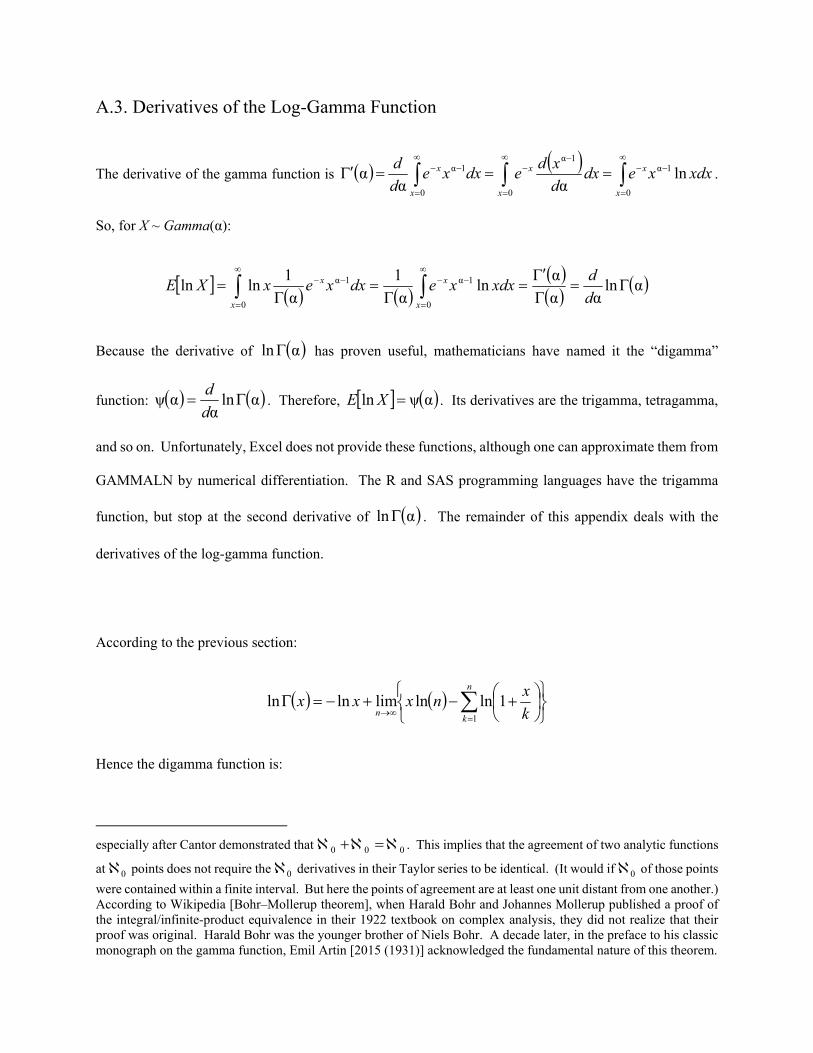
A.3. Derivatives of the Log-Gamma Function

The derivative of the gamma function is

0

1α

0

1α

0

1α lnαα

αx

x

x

x

x

x xdxxedxd

xdedxxe

d

d.

So, for X ~ Gamma(α):

αln

αα

αln

α

1

α

1lnln

0

1α

0

1α

d

dxdxxedxxexXE

x

x

x

x

Because the derivative of αln has proven useful, mathematicians have named it the “digamma”

function: αlnα

αψ d

d. Therefore, αψln XE . Its derivatives are the trigamma, tetragamma,

and so on. Unfortunately, Excel does not provide these functions, although one can approximate them from

GAMMALN by numerical differentiation. The R and SAS programming languages have the trigamma

function, but stop at the second derivative of αln . The remainder of this appendix deals with the

derivatives of the log-gamma function.

According to the previous section:

n

kn k

xnxxx

1

1lnlnlimlnln

Hence the digamma function is:

                                                            

especially after Cantor demonstrated that 000 . This implies that the agreement of two analytic functions

at 0 points does not require the 0 derivatives in their Taylor series to be identical. (It would if 0 of those points

were contained within a finite interval. But here the points of agreement are at least one unit distant from one another.) According to Wikipedia [Bohr–Mollerup theorem], when Harald Bohr and Johannes Mollerup published a proof of the integral/infinite-product equivalence in their 1922 textbook on complex analysis, they did not realize that their proof was original. Harald Bohr was the younger brother of Niels Bohr. A decade later, in the preface to his classic monograph on the gamma function, Emil Artin [2015 (1931)] acknowledged the fundamental nature of this theorem.

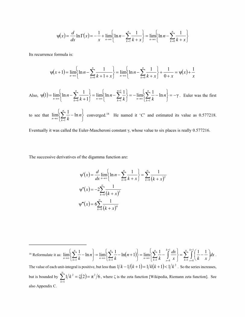
n

kn

n

kn xk

nxk

nx

xdx

dx

01

1lnlim

1lnlim

1lnψ

Its recurrence formula is:

x

xxxk

nxk

nxn

kn

n

kn

1ψ

0

11lnlim

1

1lnlim1ψ

00

Also, γln1

lim1

lnlim1

1lnlim1ψ

1

1

10

nkk

nk

nn

kn

n

kn

n

kn

. Euler was the first

to see that

n

k

n

kn

ln1

lim1

converged.18 He named it ‘C’ and estimated its value as 0.577218.

Eventually it was called the Euler-Mascheroni constant γ, whose value to six places is really 0.577216.

The successive derivatives of the digamma function are:

04

03

02

0

16ψ

12ψ

11lnlimψ

k

k

k

n

kn

xkx

xkx

xkxkn

dx

dx

                                                            

18 Reformulate it as:

1

11

111

111lim1ln

1limln

1lim

k

k

kx

k

kx

n

kn

n

kn

n

kn

dxxkx

dx

kn

kn

k.

The value of each unit-integral is positive, but less than 2111111 kkkkk . So the series increases,

but is bounded by 6π2ζ1 2

1

2

k

k , where ζ is the zeta function [Wikipedia, Riemann zeta function]. See

also Appendix C.

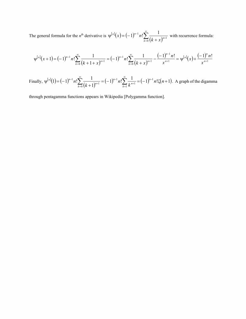
The general formula for the nth derivative is

01

1 1!1ψ

kn

nn

xknx with recurrence formula:

11

1

01

1

01

1 !1ψ

!11!1

1

1!11ψ

n

nn

n

n

kn

n

kn

nn

x

nx

x

n

xkn

xknx

Finally,

1ζ!11

!11

1!11ψ 1

11

1

01

1

nnk

nk

n n

kn

n

kn

nn . A graph of the digamma

through pentagamma functions appears in Wikipedia [Polygamma function].

Appendix B

Moments Versus Cumulants19

Actuaries and statisticians are well aware of the moment generating function (mgf) of random variable X:

X

txtXX dxxfeeEtM

Obviously, 110 EM X . It is called the moment generating function because its derivatives at zero,

if convergent, equal the (non-central) moments of X, i.e.:

nXn

tn

tXn

t

tXn

nn

X XEeXEdt

edEeE

dt

dM

0

00

0 .

The moment generating function for the normal random variable is 2σ

σ,μ

22

2tt

NetM . The mgf of a

sum of independent random variables equals the product of their mgfs:

tMtMeEeEeeEeEtM YXtYtXtYtXYXt

YX

The cumulant generating function (cgf) of X, or tXψ is the natural logarithm of the moment generating

function. So 00ψ X ; and for independent summands:

tttMtMtMtMtMt YXYXYXYXYX ψψlnlnlnlnψ

The nth cumulant of X, or Xnκ , is the nth derivative of the cgf evaluated at zero. The first two cumulants

are identical to the mean and the variance:

                                                            19 For moment generating functions see Hogg [1984, pp. 39f] and Klugman [1998, §3.9.1]. For cumulants and their generation see Daykin [1994, p. 23] and Halliwell [2011, §4].

XVarXEXEXEtM

tMtMtMtM

tM

tM

dt

dX

XEtM

tM

dt

tMdX

tX

XXXX

tX

X

tX

X

t

X

2

0

2

0

2

001

κ

lnκ

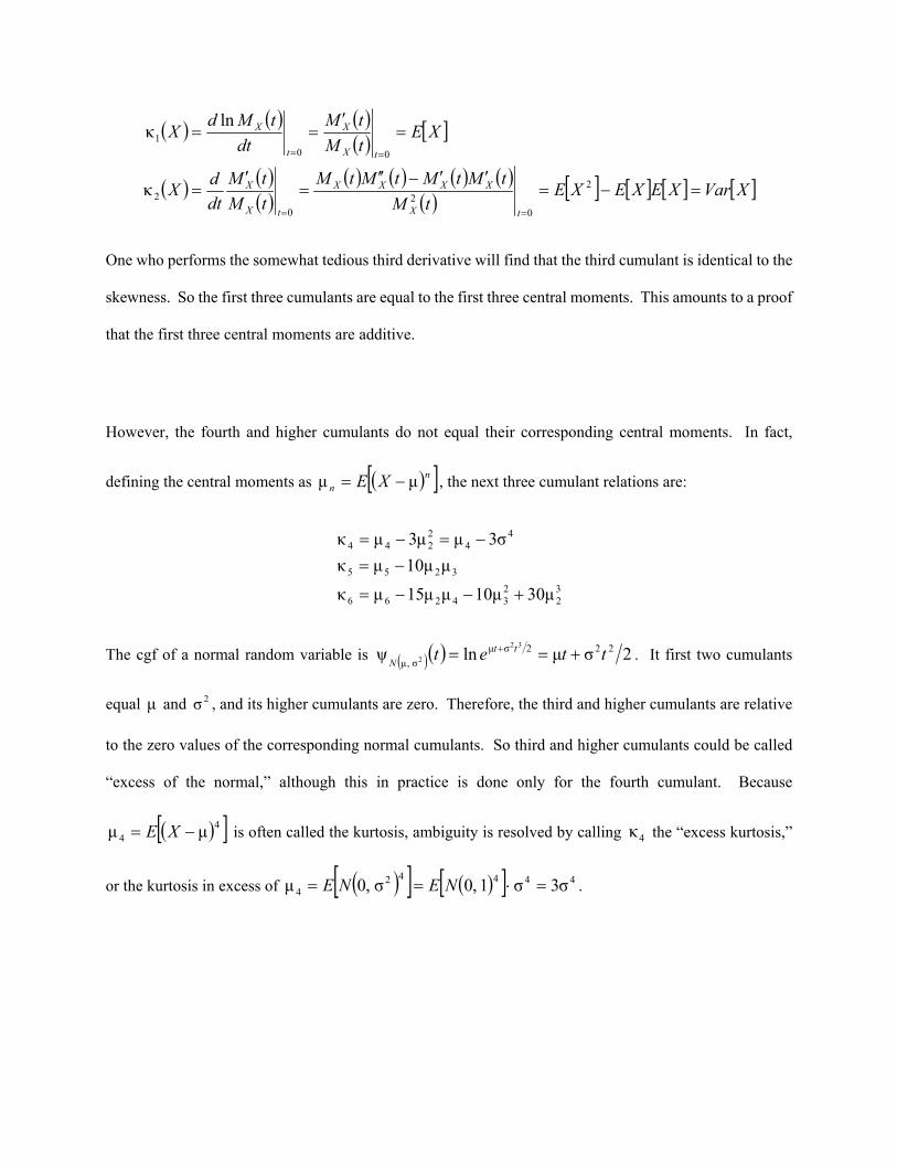
One who performs the somewhat tedious third derivative will find that the third cumulant is identical to the

skewness. So the first three cumulants are equal to the first three central moments. This amounts to a proof

that the first three central moments are additive.

However, the fourth and higher cumulants do not equal their corresponding central moments. In fact,

defining the central moments as nn XE μμ , the next three cumulant relations are:

32

234266

3255

44

2244

μ30μ10μμ15μκ

μμ10μκ

σ3μμ3μκ

The cgf of a normal random variable is 2σμlnψ 222σμ

σ,μ

32

2 ttet tt

N . It first two cumulants

equal μ and 2σ , and its higher cumulants are zero. Therefore, the third and higher cumulants are relative

to the zero values of the corresponding normal cumulants. So third and higher cumulants could be called

“excess of the normal,” although this in practice is done only for the fourth cumulant. Because

44 μμ XE is often called the kurtosis, ambiguity is resolved by calling 4κ the “excess kurtosis,”

or the kurtosis in excess of 444424 σ3σ1,0σ,0μ NENE .

Appendix C

Log-gamma Convergence

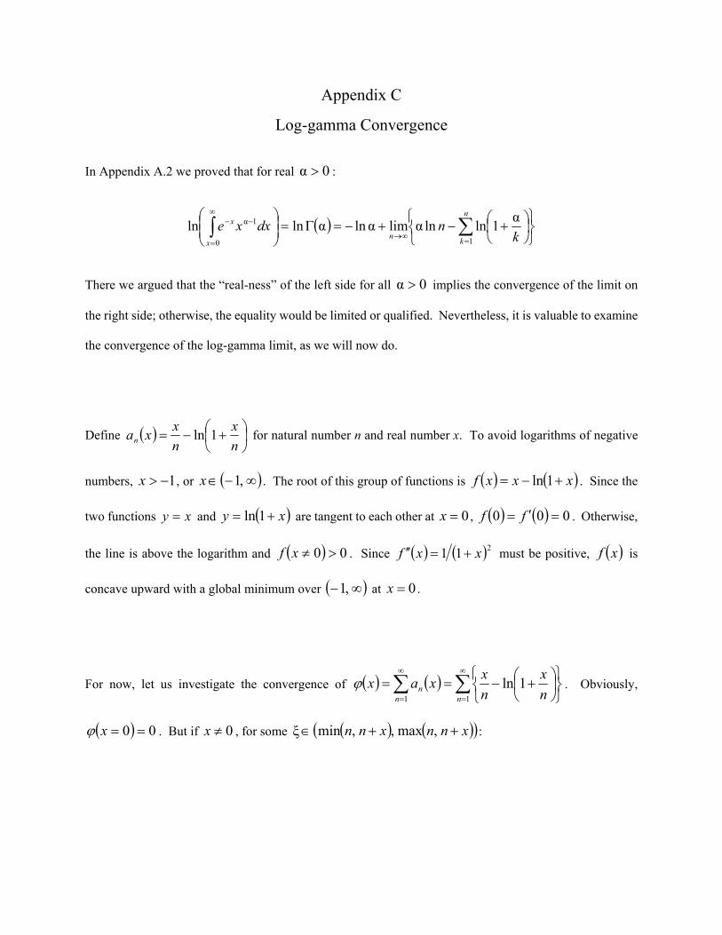
In Appendix A.2 we proved that for real 0α :

n

kn

x

x

kndxxe

10

1α α1lnlnαlimαlnαlnln  

There we argued that the “real-ness” of the left side for all 0α implies the convergence of the limit on

the right side; otherwise, the equality would be limited or qualified. Nevertheless, it is valuable to examine

the convergence of the log-gamma limit, as we will now do.

Define

n

x

n

xxan 1ln for natural number n and real number x. To avoid logarithms of negative

numbers, 1x , or ,1x . The root of this group of functions is xxxf 1ln . Since the

two functions xy and xy 1ln are tangent to each other at 0x , 000 ff . Otherwise,

the line is above the logarithm and 00 xf . Since 211 xxf must be positive, xf is

concave upward with a global minimum over ,1 at 0x .

For now, let us investigate the convergence of

11

1lnnn

n n

x

n

xxax . Obviously,

00 x . But if 0x , for some xnnxnn ,max,,minξ :

ξ

11

ξ

ξ

1

ln

1ln

nx

x

n

x

nxnn

x

u

du

n

x

n

xn

n

x

n

x

n

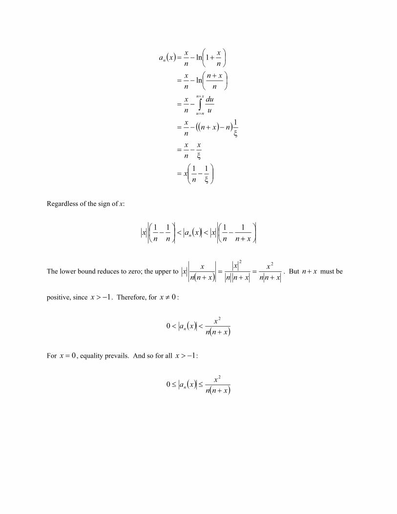
xxa

xn

nu

n

Regardless of the sign of x:

xnnxxa

nnx n

1111

The lower bound reduces to zero; the upper to xnn

x

xnn

x

xnn

xx

22

. But xn must be

positive, since 1x . Therefore, for 0x :

xnn

xxan

2

0

For 0x , equality prevails. And so for all 1x :

xnn

xxan

2

0

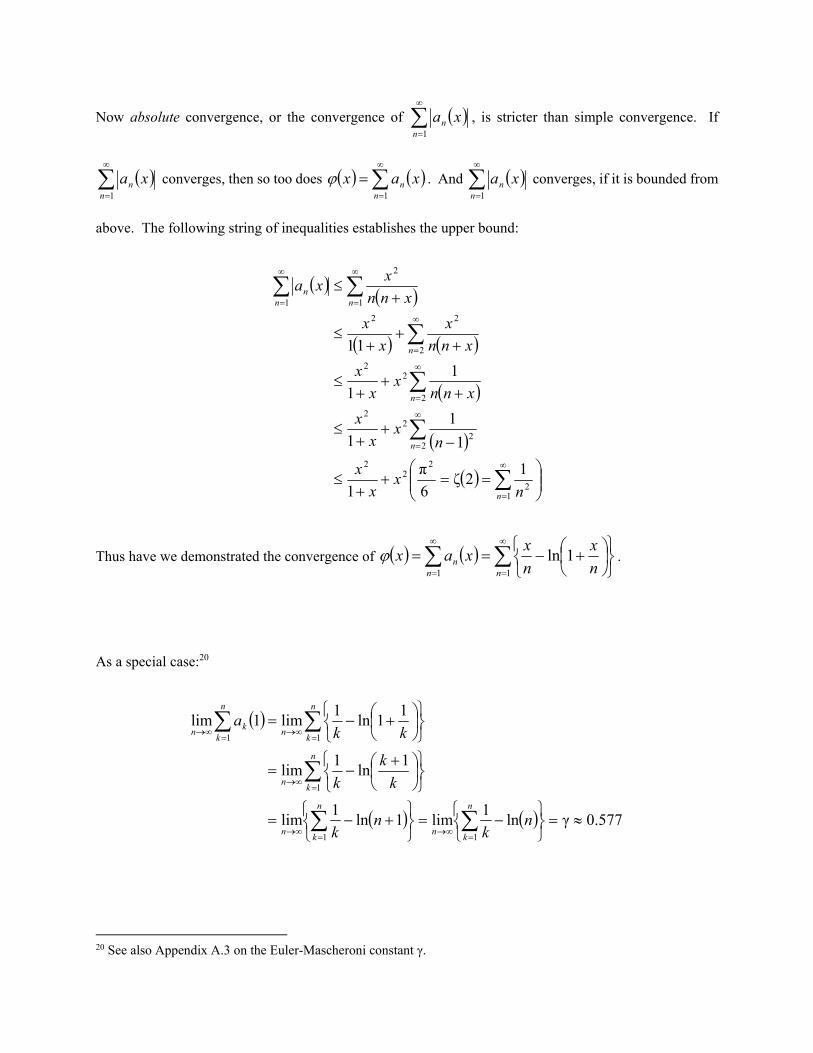
Now absolute convergence, or the convergence of

1nn xa , is stricter than simple convergence. If

1nn xa converges, then so too does

1n

n xax . And

1nn xa converges, if it is bounded from

above. The following string of inequalities establishes the upper bound:

12

22

2

22

22

2

22

2

22

1

2

1

12ζ

6

π

1

1

1

1

1

1

11

n

n

n

n

nnn

nx

x

x

nx

x

x

xnnx

x

x

xnn

x

x

x

xnn

xxa

Thus have we demonstrated the convergence of

11

1lnnn

n n

x

n

xxax .

As a special case:20

0.577γln1

lim1ln1

lim

1ln

1lim

11ln

1lim1lim

11

1

11

n

kn

n

kn

n

kn

n

kn

n

kk

n

nk

nk

k

k

k

kka

                                                            20 See also Appendix A.3 on the Euler-Mascheroni constant γ.

Returning to the limit in the log-gamma formula and replacing ‘α’ with ‘x’, we have:

n

kk

n

k

n

kn

n

k

n

kn

n

kn

n

kn

xaγx

k

x

k

xn

kx

k

x

k

x

k

xnx

k

x

k

x

k

xnx

k

xnx

1

11

11

11

1lnln1

lim

1lnlnlim

1lnlnlim1lnlnlim

 

Thus, independently of the integral definition, we have proven for 0α the convergence of

n

kn k

n1

α1lnlnαlimαlnαln .21

This is but one example of a second-order convergence. To generalize, consider the convergence of

n

kn k

xfx

1

lim . As with the specific xxxf 1ln above, the general function f must be

analytic over an open interval about zero, ba 0 . Likewise, its value and first derivative at zero must

be zero, i.e., 000 ff . According to the second-order mean value theorem, for bax , , there

exists a real ξ between zero and x such that:

                                                            21 Actually. we proved the convergence of the second term, the one with the limit, for 1α . It is the first term,

the logarithm, that contracts the domain of αln to 0α . As a complex function zln converges for all

complex ,2,1,0 z . However, zln is multivalent, or unique only to an integral multiple of iπ2 . That

exponentiation removes this multivalence is the reason why ze z ln is analytic, except at

,2,1,0 z . The infinite product

n

zzz

ez

nz

n1

11

limln

converges, unless some factor in the

denominator equals zero, i.e., unless ,2,1,0 z .

22

2

ξ

2

ξ00 x

fx

fxffxf

Therefore, there exist kξ between zero and k

x such that

n

k

k

n

n

kn k

xf

k

xfx

1

2

1 2

ξlimlim .

Again, we appeal to absolute convergence. If

n

k

k

n

n

k

k

n k

fx

k

xf

12

2

1

2 ξlim

22

ξlim converges, then

x converges. But every kξ belongs to the closed interval Ξ between 0 and x. And since f is analytic

over ba, , f is continuous over Ξ. Since a continuous function over a closed interval is bounded,

Mf k ξ0 for some real M. So, at length:

6

π2ζ

1limlim

ξlim0

2

12

12

12

MMk

Mk

M

k

f n

kn

n

kn

n

k

k

n

Consequently,

n

kn k

xf

1

lim converges to a real number for every function f that is analytic over some

domain about zero and for which 000 ff . The convergence must be at least of the second order;

a first-order convergence would involve

n

kn k

M

1

lim and the divergence of the harmonic series.

The same holds true for analytic functions over complex domains. Another potentially important second-

order convergence is

n

k

k

z

n k

zez

1

1lim .