Embed Size (px)
Citation preview
IEEE/ACM TRANSACTIONS ON NETWORKING, VOL. 14, NO. 6, DECEMBER 2006 1153
The Random Trip Model: Stability, StationaryRegime, and Perfect Simulation
Jean-Yves Le Boudec, Fellow, IEEE, and Milan Vojnovic, Member, IEEE
Abstract—We define “random trip”, a generic mobility modelfor random, independent node motions, which contains as specialcases: the random waypoint on convex or nonconvex domains,random walk on torus, billiards, city section, space graph, inter-city and other models. We show that, for this model, a necessaryand sufficient condition for a time-stationary regime to exist isthat the mean trip duration (sampled at trip endpoints) is finite.When this holds, we show that the distribution of node mobilitystate converges to the time-stationary distribution, starting fromthe origin of an arbitrary trip. For the special case of randomwaypoint, we provide for the first time a proof and a sufficient andnecessary condition of the existence of a stationary regime, thusclosing a long standing issue. We show that random walk on torusand billiards belong to the random trip class of models, and estab-lish that the time-limit distribution of node location for these twomodels is uniform, for any initial distribution, even in cases wherethe speed vector does not have circular symmetry. Using Palm cal-culus, we establish properties of the time-stationary regime, whenthe condition for its existence holds. We provide an algorithm tosample the simulation state from a time-stationary distributionat time 0 (“perfect simulation”), without computing geometricconstants. For random waypoint on the sphere, random walk ontorus and billiards, we show that, in the time-stationary regime,the node location is uniform. Our perfect sampling algorithm isimplemented to use with ns-2, and is available to download fromhttp://ica1www.epfl.ch/RandomTrip.
Index Terms—Mobility models, random waypoint, simulation.
I. INTRODUCTION
RANDOM mobility models have been used extensivelyto evaluate performance of networking systems in both
mathematical analysis and simulation based studies. The goalof our work is twofold: 1) provide a class of “stable” mobilitymodels that is rich enough to accommodate a large variety ofexamples and 2) provide an algorithm to run “perfect simu-lation” of these models. Both goals are motivated by recentfindings about the random waypoint; this is an apparentlysimple model that fits in our framework, the simulation ofwhich was reported to pose a surprising number of challenges,such as speed decay, a change in the distribution of locationand speed as the simulation progresses [11], [16], [22], [24].
Manuscript received March 3, 2006; approved by IEEE/ACM TRANSACTIONS
ON NETWORKING Editor E. Knightly. A conference version of this paper ap-peared in the IEEE INFOCOM 2005, Miami, FL, March 2005, under the title“Perfect Simulation and Stationarity of a Class of Mobility Models.”
J.-Y. Le Boudec is with the EPFL, CH-1015 Lausanne, Switzerland (e-mail:[email protected]).
M. Vojnovic is with Microsoft Research Ltd., CB3 0FB Cambridge, U.K.(e-mail: [email protected]).
Digital Object Identifier 10.1109/TNET.2006.886311
A. Random Trip Model
We define “random trip”, a model of random, independentnode movements. Such independent node movements are en-tirely defined by specifying random process of movement for asingle node. The model does not directly accommodate groupmobility models, which are left for further study. The randomtrip model is defined by a set of “stability” conditions for a nodemovement. These conditions guarantee existence of a time-sta-tionary regime of node mobility state or its nonexistence. Theyalso guarantee convergence of node mobility state to a time-sta-tionary regime, whenever one exists, starting a node movementfrom origin of a trip. The reported observations for random way-point such as that speed vanishes to 0 as simulation progresses(“considered harmful” [23]) are in fact all related to the set ofproblems on stability of random processes that include findingconditions for existence of a stationary regime or its nonexis-tence. Stability problems also include finding conditions underwhich convergence to a stationary regime is guaranteed, when-ever there exists one. These conditions are important to alleviatenondesirable situations such as the reported vanishing of nodenumerical speed to 0.
In the absence of established properties of real mobility pat-terns, it is not yet clear today what the requirements on mobilitymodels should be [10]. The random trip model is a broad classof independent node movements that can be appropriately pa-rameterized to synthesize an a priori assumed mobile behavior.
B. Random Trip Examples
We show in Section III that many examples of randommobility models used in practice are random trip models.Our catalog includes examples such as classical random way-point, city driving models (“space graph” [13], “city section”or “hierarchical random waypoint” [6]), circulation models(“random waypoint on sphere”), or the special purpose “fishin a bowl” and “Swiss flag”. These are all accommodated bythe “restricted random waypoint” introduced in Section III-D.These examples illustrate well the geometric diversity of mo-bility domains: for models such as “Swiss flag” we have anonconvex area on a plane; for models such as “space graph”or “city section”, a concatenation of line segments that repre-sent streets; for “random waypoint on sphere”, a surface in athree-dimensional space.
In some cases, it is desirable to assume that in steady-state,node location is uniformly distributed on a domain. This is pro-vided by “random walk on torus” and “billiards”, which are de-fined by “bending” the paths of node movement with wrappingand billiards-like reflections, respectively, in a rectangular area
1063-6692/$20.00 © 2006 IEEE
1154 IEEE/ACM TRANSACTIONS ON NETWORKING, VOL. 14, NO. 6, DECEMBER 2006
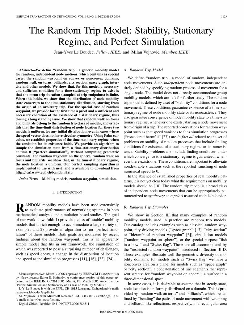
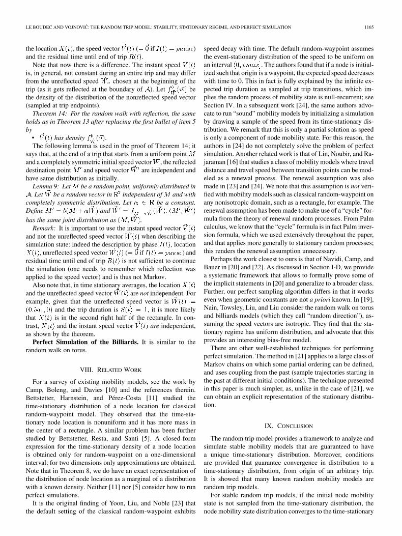
Fig. 1. Mobility on a “space graph” as introduced by Jardosh et al. [13]. Amobile initiates a trip from a vertex and moves along a shortest-path to a ran-domly chosen destination vertex. This model is discussed in Section III-D2. Thealternative, called city section (Section III-C2), chooses the trip end-points onany point of the domain defined by the line segments of the graph edges. Thespatial graph is either generated synthetically (e.g., [13]) or constructed fromreal-world street maps. The numeric speeds can be assigned to the edges of agraph.
on a plane. “Random waypoint on a sphere” is another such ex-ample, embedded in three dimensions.
C. Perfect Simulation
Like many simulation models, when the condition for sta-bility is satisfied, simulation runs go through a transient pe-riod and converge to the stationary regime. It is important toremove the transients for performing meaningful comparisonsof, for example, different mobility regimes. A standard methodfor avoiding such a bias is to 1) make sure the used model has astationary regime and 2) remove the beginning of all simulationruns in the hope that long runs converge to stationary regime.
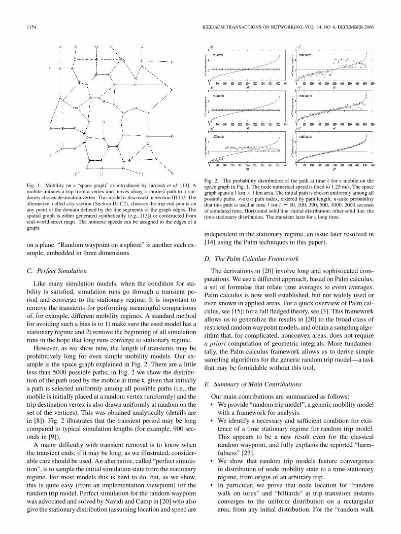
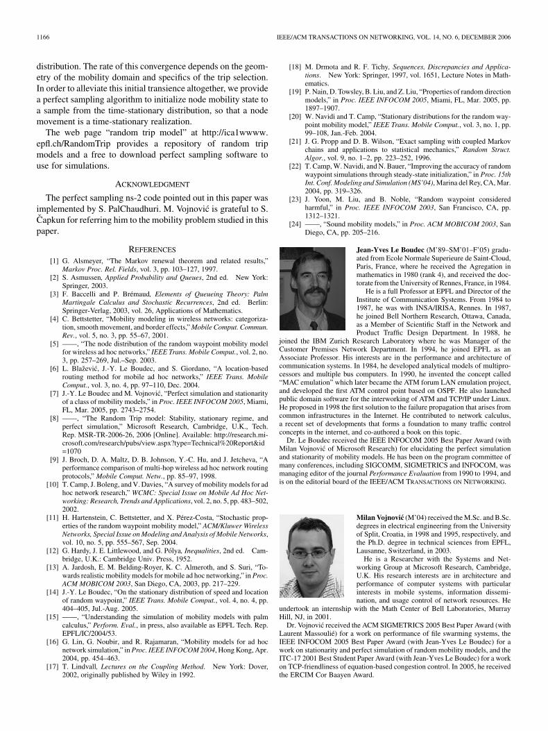
However, as we show now, the length of transients may beprohibitively long for even simple mobility models. Our ex-ample is the space graph explained in Fig. 2. There are a littleless than 5000 possible paths; in Fig. 2 we show the distribu-tion of the path used by the mobile at time , given that initiallya path is selected uniformly among all possible paths (i.e., themobile is initially placed at a random vertex (uniformly) and thetrip destination vertex is also drawn uniformly at random on theset of the vertices). This was obtained analytically (details arein [8]). Fig. 2 illustrates that the transient period may be longcompared to typical simulation lengths (for example, 900 sec-onds in [9]).
A major difficulty with transient removal is to know whenthe transient ends; if it may be long, as we illustrated, consider-able care should be used. An alternative, called “perfect simula-tion”, is to sample the initial simulation state from the stationaryregime. For most models this is hard to do, but, as we show,this is quite easy (from an implementation viewpoint) for therandom trip model. Perfect simulation for the random waypointwas advocated and solved by Navidi and Camp in [20] who alsogive the stationary distribution (assuming location and speed are
Fig. 2. The probability distribution of the path at time t for a mobile on thespace graph in Fig. 1. The node numerical speed is fixed to 1.25 m/s. The spacegraph spans a 1 km� 1 km area. The initial path is chosen uniformly among allpossible paths. x-axis: path index, ordered by path length; y-axis: probabilitythat this path is used at time t for t = 50, 100, 300, 500, 1000, 2000 secondsof simulated time. Horizontal solid line: initial distribution; other solid line: thetime-stationary distribution. The transient lasts for a long time.
independent in the stationary regime, an issue later resolved in[14] using the Palm techniques in this paper).
D. The Palm Calculus Framework
The derivations in [20] involve long and sophisticated com-putations. We use a different approach, based on Palm calculus,a set of formulae that relate time averages to event averages.Palm calculus is now well established, but not widely used oreven known in applied areas. For a quick overview of Palm cal-culus, see [15]; for a full fledged theory, see [3]. This frameworkallows us to generalize the results in [20] to the broad class ofrestricted random waypoint models, and obtain a sampling algo-rithm that, for complicated, nonconvex areas, does not requirea priori computation of geometric integrals. More fundamen-tally, the Palm calculus framework allows us to derive simplesampling algorithms for the generic random trip model—a taskthat may be formidable without this tool.
E. Summary of Main Contributions
Our main contributions are summarized as follows:• We provide “random trip model”, a generic mobility model
with a framework for analysis.• We identify a necessary and sufficient condition for exis-
tence of a time stationary regime for random trip model.This appears to be a new result even for the classicalrandom waypoint, and fully explains the reported “harm-fulness” [23].
• We show that random trip models feature convergencein distribution of node mobility state to a time-stationaryregime, from origin of an arbitrary trip.
• In particular, we prove that node location for “randomwalk on torus” and “billiards” at trip transition instantsconverges to the uniform distribution on a rectangulararea, from any initial distribution. For the “random walk
LE BOUDEC AND VOJNOVIC: THE RANDOM TRIP MODEL: STABILITY, STATIONARY REGIME, AND PERFECT SIMULATION 1155
on torus” model, the result requires a mild assumption onthe distribution of the node speed vector (essentially, thatit has a density) whereas previous results in [19] requiredthe circular symmetry (speed vector is isotropic). For the“billiards” model, we require that the speed vector has acompletely symmetric distribution (Section III-G), whichmeans that it goes up or down [resp. left or right] withequal probability. This is also a weaker assumption thanthe circular symmetry required in [19].
• We show that for three examples (random walk on torus,billiards, random waypoint on sphere) the node location isuniform in steady-state. For the random walk on torus, thesteady state is essentially the same as the naive initializa-tion (with uniform node placement) and there is no speeddecay. In contrast, there is speed decay for random way-point on a sphere.
• We provide an algorithm to initialize node mobility stateso that the distribution of the node state is time-stationarythroughout a simulation (“perfect simulation”).
• The perfect sampling algorithm (i) accommodates randomwaypoint models on nonconvex areas and (ii) avoids com-putation of geometric integrals when they are difficult tocompute.
F. Organization of the Paper
The random trip model is defined in Section II, along witha notation list. Section III provides a broad catalog of randommobility models and shows that all are random trip models.In particular, that section contains convergence results for“random walk on torus” and “billiards” random trip models.The main result on stability is the necessary and sufficient con-dition for existence and uniqueness of a time-stationary regime,and convergence to this regime, whenever it exists, is givenin Section IV. In Section V, we give a generic representationof the time stationary distribution of any random trip modelthat satisfies the stability condition. In Section VI, we derivean efficient sampling algorithm for perfect simulation for thesub-family of models that can be represented as restrictedrandom waypoint. In Section VII, we show that, for randomwaypoint on sphere, random walk on torus and billiards, thetime-stationary distribution of node location is uniform, i.e., thedistribution bias for location does not exist for these models.In Section VIII, we discuss related work. Section IX providesconcluding remarks. Most of the proofs are deferred to [8,Appendix], and are in some cases only briefly hinted in themain text.
II. THE RANDOM TRIP MODEL DEFINITION
The random trip mobility model is defined by the followingframework.
A. Trip, Phase, Path
1) Domain: The domain is a subset of , for some integer.
2) Phase: is a set of phases on , for some integer. A phase describes some state of the mobile, specific to the
model. For example, it may indicate whether the mobile movesor pauses at a given time.
3) Path: is a set of paths on . A path is a continuousmapping from [0,1] to that has a continuous derivative exceptmaybe at a finite number of points (this is necessary to definethe speed).
For , is the origin of , is its destination, andis the point on attained when a fraction of the
path is traversed.4) Trip: A trip is specified by a path and a duration .
The position of the mobile at time is defined iteratively asfollows. There is a set , of transition instants,such that . At time , a phase ,a path and a trip duration are drawn accordingto some specified trip selection rule, specific to the model. Thenext transition instant is and the position ofthe mobile is
The trip selection rule is constrained to choose a path suchthat . Further, we assume that, with proba-bility 1, the duration of the trip is positive (instantaneoustransitions are not allowed).
Following a customary convention, whenever we consider astationary realization of node mobility, we extend the transitioninstants to the entire line , and enumerate them as
. In these cases, 0 is an arbitrarytime.
5) Default Initialization Rule: At time , a phase, path,position on the path, and remaining time until the next transitionare drawn according to some specified initialization rule. Wedefine as a default initialization rule that which takes time 0 asthe first transition instant , and selects a phase, pathand trip duration according to the trip selection rule. The defaultinitialization rule has been used in simulations of many randommobility models (e.g., classical random waypoint).
We introduce additional assumptions. Some of the assump-tions are either trivial to verify or always hold in real world,while some are crucial to guarantee stability of the random tripmodel and may not be always trivial to verify. This is discussedmore concretely in Section II-D. In any case, the followingassumptions accommodate a broad class of random mobilitymodels.
B. Conditions on Phase and Path
(H1) with defined as a coupleof phase and path is a Markov chain on .
(H2) The chain is Harris recurrent [17, sec. III.9]: Thereexists a set , a probability measure with supporton , a number , and an integer such thatthe following two conditions hold
(i) for some for all(ii) for all and any measur-
able in .Here we use the notation , .
Condition i implies that is a recurrent set of the chain. Con-dition ii says that is a regeneration set in the sense that the
1156 IEEE/ACM TRANSACTIONS ON NETWORKING, VOL. 14, NO. 6, DECEMBER 2006
conditional probability that the chain hits a set , after tran-sitions from , is lower bounded by that isindependent of .
Condition H2 ensures the chain has a unique stationarymeasure (up to a multiplicative constant) defined by
(1)
where is the transition semi-group of the chain.
(H3) The chain is positive Harris recurrent, i.e., H2 holdsand the number of transitions between successive visits to theset has a finite expectation.
Condition H3 implies the invariant measure is such that, so that it can be normalized to a probability
distribution.
C. Conditions on Trip Duration
(H4) Three hypotheses:(i) The distribution of a trip duration , given the phase
and path , is independent of any other past and .Formally, we have1
for all
We assume that for all , is a nondefec-tive probability distribution, that is
, for all . Note that in general the trip durationis dependent on the path .
(ii) Each trip takes a strictly positive time, i.e.
all and almost all
This condition is always true in reality.(iii) The Markov renewal process is nonarith-
metic, i.e., there exists no and some “shift” functionsuch that given , takes values
on the set , for almost all .This assumption is automatically true if there is a subset
of strictly positive probability such that,given , the distribution of has a density, i.e.,
, for some function , and.
Condition H4.iii is needed to state the convergence in distri-bution to a time-stationary distribution as specified in Theorem6, item ii, for sample paths initialized at as specified bythe default initialization rule (see item 5 in Section II-A).2
1Throughout the paper, we use the subscript 0 to signify that the distributionor density or expectation is of the state embedded at trip transition instants.
2Condition H4.iii is not needed for existence and uniqueness of a time sta-tionary distribution (Theorem 6, item i, Section IV) and one can indeed con-struct time-stationary sample paths of mobility when H4.iii does not hold byappropriate initialization.
Notation Used in Section II
• : model domain, connected and bounded.• length of shortest path in from to
; if is convex .• : th transition time, at which a new trip is defined• Phase: ; Trip origin location: , Trip path:
; Trip duration: . The subscriptdenotes th trip with first trip labeled with .
• , , , ,: phase, starting point, path, trip duration for
the trip used by mobile at time , location at time .and if then ,
and .• : fraction of the current trip that was already
traversed. Thus, is the time elapsed on thecurrent trip and the location of the mobile at time is
, with . We assume that thespeed is constant on a trip, i.e., if then
(but speedmay be different for distinct trips).
• It follows that the speed vector of the mobile at a time thatis not an end of trip is ,with and the numerical speed is .
• For some random variable , is the “Palmexpectation”, which can be interpreted as the expectation,conditional to the event that a transition occurs at time0, when the system has a stationary regime. denotesthe event average viewpoint [3], [15]. For example
is the average trip duration; incontrast, when the system has reached steady-state,
is the average duration of a trip,seen from an observer who samples the system at anarbitrary point in time. Both are usually different becausethe observer is more likely to sample a large trip duration.
• In order to simplify notation and at no expense ofambiguity, for a right-continuous process , ,and appropriately defined function , we write
for the Palm expectation ; herewith a trip transition instant.
• We say a property holds for almost all , if it holds forall , but maybe not for some that lies in a setof zero measure.
D. How to Verify the Conditions in Practice?
Condition H1 is a structural assumption on the trip selectionover time and is easy to verify; the same holds for H4.i and H4.ii.
Condition H4.iii is true as soon as the trip duration has a den-sity, for a non-negligible subset of paths and phases. In practice,trip durations either have a density or are mixtures of constants.It is sufficient that, for some (non-negligible) subset of path andphase conditions, the trip duration has a density. For example,H4.iii is true for a model with pauses if either the pause dura-tion, or the (nonpause) trip duration has a density.
LE BOUDEC AND VOJNOVIC: THE RANDOM TRIP MODEL: STABILITY, STATIONARY REGIME, AND PERFECT SIMULATION 1157
Conditions H2 and H3 are stronger. They essentially say thatthe Markov chain of system states, sampled at trip endpoints,is stable, in a strong sense. The technical difficulty here is that,for many examples, we have a Markov chain on a noncount-able state space, for which stability conditions are mathemat-ically complicated. However, it helps to think that for randomtrip with a countable state space , conditions H2 and H3simply mean positive recurrence. For a finite state space, theyeven more simply mean that the state space is connected.
We next show that conditions H1–H4 are verified by manyrandom mobility models.
III. EXAMPLES
We give a nonexhaustive catalog of example random mobilitymodels and show they are all random trip models.
A. Classical Random Waypoint With Pauses
This is the classical random waypoint model. is assumedto be convex ( is a rectangle or a disk in [10], [11]). Pathsare straight line segments: for thesegment with endpoints and . Pauses are special cases ofpaths, when endpoints are equal: . There are twophases . At a transition instant, the tripselection rule alternates the phase from to or viceversa. If the new phase is , the trip duration is drawnfrom the distribution ; the path is a pause at thecurrent point. If the new phase is , the trip selection rulespicks a point at random uniformly in , and a numericalspeed according to the density . A classical choice(uniform speed) is . Thetrip duration is then and the pathis the segment . The default initialization rule startsthe model at the beginning of a pause, at a location uniformlychosen in .
Theorem 1: The random waypoint with pauses is a randomtrip model.
Proof: H1 and H4 obviously hold. By Theorem 2 shownnext it is sufficient to consider the model without pauses. Thedriving chain is now and is indeedMarkov. Take as recurrent set so that condition H2.iobviously holds. The paths are selected such that andare independent for . It follows that for anyand any
where is the uniform distribution on , defined by. This shows that H2.ii holds with
(product measure) and any . Therecurrent set is visited at each transition, so H3 is indeedtrue.
This model is well known; its stationary properties are studiedin [11], [14], and [22]. However, even for this simple model ourframework provides two new results: the proof of existence of astationary regime (Section IV), and a sampling algorithm for thestationary distribution over general areas that does not requirethe computation of geometric integrals (Section VI).
B. Adding Pauses to a Model
Assume we have a random trip model with phases andpaths . We can add pauses to this model and obtain a newmodel as follows. At the end of the th trip, a pause time
is drawn at random, depending only (possibly) on the currenttrip and phase. This means that the pause duration at the end ofthe th trip, conditional on all past, depends only on and .
In we have phases and paths given by (for all):
(2)
where is the path that remains entirely at point(i.e., for ).
Theorem 2: If is a random trip model, then is also arandom trip model.
Proof: It is straightforward to show that assumptions H1and H4 hold. We now show H2.i. Let be a regeneration setfor model , which by hypothesis exists. Let
Let be the sequence that alternatesbetween and , and indicates whether the thtrip is a pause or not. The driving chain in model is
. If (this is implicitly assumed in (2)) thenand thus
for some
for some
for some
and similarly
for some
for some
for some
which shows H2.i.To show H2.ii, let , , be such that
for all and any measurable in . De-fine the probability measure on by
and . Wehave, for :
and for :
which shows H2.ii.
C. Random Waypoint on General Connected Domain
This is a variant of the classical random waypoint (ExampleIII-A), where we relax the assumption that is convex, butassume that is a connected domain over which a uniformdistribution is well defined. For two points , in , we call
the distance from to in , i.e., the minimum lengthof a path entirely inside that connects and . is theset of shortest paths between endpoints. The trip selection rule
1158 IEEE/ACM TRANSACTIONS ON NETWORKING, VOL. 14, NO. 6, DECEMBER 2006
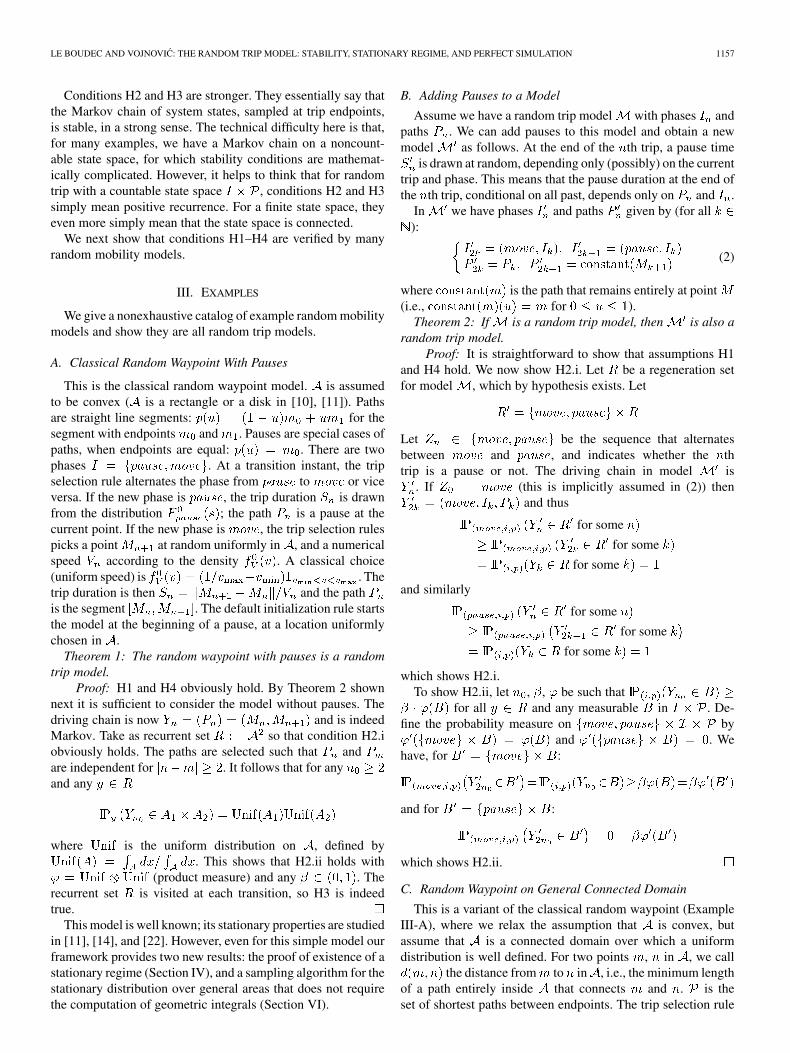
Fig. 3. Random waypoint on a nonconvex domain (Swiss Flag). A trip is theshortest path inside the domain from a waypoint M to the next. WaypointsM are drawn uniformly in the domain. In figure, the shortest pathM ,Mhas two segments, with a breakpoint at K; the shortest paths M , M andM , M have one segment each. M(t) is the current position.
Fig. 4. A restricted random waypoint on a plane with four squares as subdo-mains. This model was introduced in [6] to simulate a wide-area routing pro-tocol. It was used as an idealized view of four towns represented by squares.A mobile moves according to random waypoint within a square for a randomnumber of visits and then picks a point uniformly at random in another ran-domly chosen square as a destination. The figure shows a sample path of themobile movement. The speed on the trip is chosen according to a distributionthat depends on the origin and destination squares.
picks a new endpoint uniformly in , and the next path is theshortest path to this endpoint. If there are several shortest paths,one of them is randomly chosen according to some probabilitydistribution on the set of shortest paths. The set of phases is
. This model fits in our framework for thesame reasons as the former example.
1) Swiss Flag: The model is random waypoint on particularnonconvex domain defined by the cross section as in Fig. 3.
2) City Section: This is a special case of random waypoint ona nonconvex domain. The domain is the union of the segmentsdefined by the edges of the space graph (e.g., Fig. 1). Arbitrarynumeric speeds can be assigned to edges of the graph. The “dis-tance” from one location to another is the travel time.
D. Restricted Random Waypoint
This model was originally introduced by Blazevic et al. [6]in a special form described in Fig. 4, in order to model intercityexamples. We define it more generally as follows.
The trip endpoints are selected on a finite set of subdomains, . The domain is a convex closure of the subdo-
mains , . The trip selection rule is described as follows.
Fig. 5. Fish in a bowl is a restricted random waypoint. A is the volume ofthe sphere comprised between two horizontal planes. Waypoints are on theboundary A of A.
To simplify, we first consider a node movement with no pauses.Suppose the node starts from a point chosen uniformly atrandom on a subdomain . The node picks the number of tripsto undergo with trip endpoints in the subdomain from a distri-bution . The next subdomain is drawn from the distribution
. At each trip transition, the node decrements by 1, aslong as , else it sets to a random sample from the dis-tribution . Then, if , the current subdomain is setto and the next subdomain to a sample from . The tripdestination is chosen uniformly at random on if , elseuniformly at random on . This process repeats. The model isextended to accommodate pauses in a straightforward mannerby inserting pauses at the trip transition instants.
The phase is , where and are respectively,the current and next subdomain, is the number of trips withboth endpoints in the subdomain , and .Given a phase , the path is the line seg-ment , with uniformly distributed on and
uniformly distributed on or , for and ,respectively.
Theorem 3: Assume that i) is an irreducible transition ma-trix, and ii) the number of trips within a subdomain has a finiteexpectation, i.e., , for all . Then,the restricted random waypoint is a random trip model.
Proof (given in [8, Appendix]) derives from known ergodicityresults for Markov chains on countable state spaces.
In addition to the model in Fig. 4, we give two particularexamples of the restricted random waypoint model.
1) Fish in a Bowl: The model is restricted random waypointon the domain defined by the volume of the bowl, as in Fig. 5.The waypoints are restricted to the subset of the domain
, where is the surface of the bowl (see Fig. 5). The setof phases is .
2) Space Graph: We defined this model in Section I.It is a special case of restricted random waypoint with
and . Note thatit differs from the City Section in that the waypoints are re-stricted to be vertices. The set of phases is .
Note that all models III-A to III-D2 and III-E are special casesof the restricted random waypoint, with , , and
for examples III-Ato III-C2, a strict subset of for
LE BOUDEC AND VOJNOVIC: THE RANDOM TRIP MODEL: STABILITY, STATIONARY REGIME, AND PERFECT SIMULATION 1159
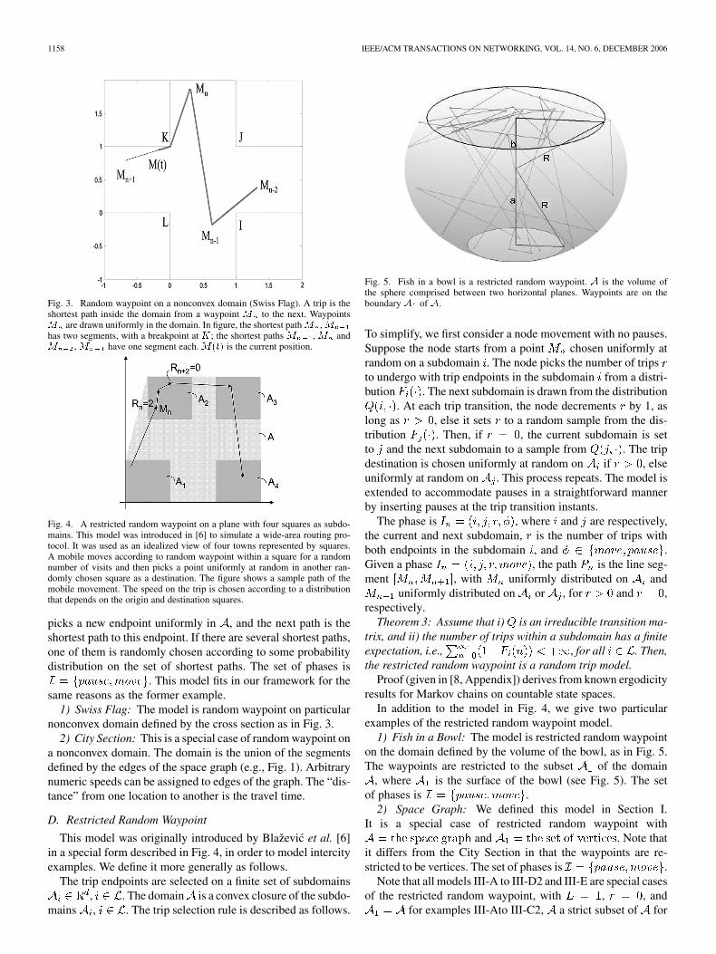
Fig. 6. Random waypoint on a sphere.
examples III-D1 and III-D2. Note that the subdomains maybe convex as in Fig. 4 or not as in Fig. 3.
E. Random Waypoint on Sphere
is the unit sphere of . is the set of shortest paths pluspauses. The shortest path between two points is the shortest ofthe arcs on the great circle that contains the two points (seeFig. 6). If the two points are on the same great circle diam-eter, the two arcs have same length (this occurs with probability0). The trip transition rule picks a path endpoint uniformly onthe sphere, and the path is the shortest path to it (if there aretwo, one is chosen with probability 0.5). The set of phases is
. The numerical speed is chosen indepen-dently. Initially, a point is chosen uniformly.
This model is in fact a special case of the random waypointon a connected, nonconvex domain. However, we mention itseparately as it enjoys special properties (the stationary locationis uniform, unlike for the random waypoint models describedearlier).
F. Random Walk on Torus
This model (e.g., [4]) is primarily used because of its sim-plicity: unlike for the random waypoint, the distribution of lo-cation and speed at a random instant are the same as at a tran-sition instant, as we show later. The model was referred to asrandom direction in [4] and [19]. We will see below that move-ment under this model is indeed a random walk on torus, hencewe refer to it as random walk on torus.
The domain is the rectangle . Paths arewrapped segments, defined as follows. The trip selection rulechooses a speed vector and a trip duration independently,according to some fixed distributions. Choosing a speed vector
is the same as choosing a direction of movement and a nu-merical speed. The mobile moves from the endpoint in thedirection and at the numeric speed given by the speed vector.When it hits the boundary of , say for example at a location
, it is wrapped to the other side, to location , from
where it continues the trip (Fig. 7). Let be thewrapping function:
(3)
The path (if not a pause) is defined by , suchthat . Note that wrapping does notmodify the speed vector (Fig. 7). After a trip, a pause time isdrawn independent of all past from some fixed distribution. Ini-tially, the first endpoint is chosen in according to some arbi-trary distribution. As we see later, the distribution of endpointtends to uniform distribution (when sampled at transition in-stants).
For , and if there are no pauses, the sequenceis a random walk on the torus, in the sense that
where is addition modulo1 (componentwise) and . This is why this mobilitymodel is itself called random walk.
Assumptions H1 and H4 are obviously satisfied by therandom walk, with set of phases . Theother assumptions of the random trip model are satisfiedmodulo some mild assumption on distributions:
Theorem 4: Assume that the distribution of the speed vectorchosen by the trip selection rule has a density (with respect
to the Lebesgue measure in ). Further assume that either thedistribution of trip durations or distribution of pause times havea density. The random walk on torus satisfies the random tripassumptions.
Remark: Note that we do not assume any form of symmetryfor the direction of the speed vector, contrary to [19].
The proof is based on a sequence of lemmas that are displayedin the rest of this subsection. The first lemma characterizes thenode location at trip end points.
Lemma 1: In the random walk without pause, the sequenceis a Harris recurrent Markov chain, with sta-
tionary distribution uniform on .The asserted convergence is proved by using the
Erdös–Turán–Koksma inequality [18, Theorem 1.21], whichyields the following result:
Lemma 2: For any ,
(4)
where the supremum is over all product intervals in andis the conditional distribution of given .
In order to apply the Erdös–Turán–Koksma inequality, weneed the following auxiliary result.
Lemma 3: Let be a real random variable that is nonlattice.For , :
(5)
Proof: We apply the Cauchy–Schwartz [12, sec. 6.5,p.132] inequality to the complex valued random variables
and 1. We have
(6)
1160 IEEE/ACM TRANSACTIONS ON NETWORKING, VOL. 14, NO. 6, DECEMBER 2006
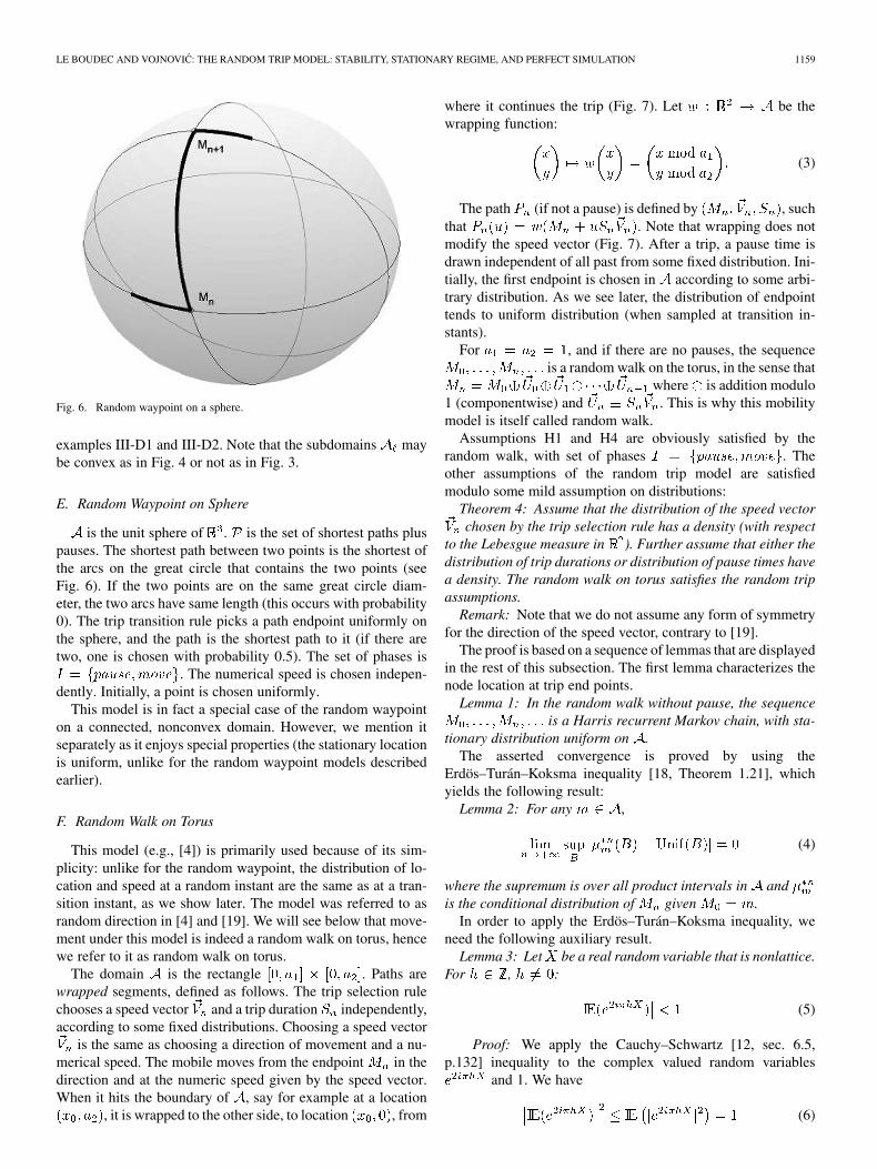
Fig. 7. Definition of random walk on torus (left) and billiards (right).
and equality implies that a.s. for some constant, and has to be lattice.
G. Billiards
This is similar to example III-F, but with billiards-like reflec-tions instead of wrapping (Fig. 7). The definition is identical toexample III-F, with the wrapping function replaced by the bil-liards reflection function , defined by
where is the 2-periodic function defined by
Unlike the wrapping function, the billiards reflection may alterthe direction of speed vector (Fig. 7). Therefore, we make a dif-ference between the unreflected speed vector and the in-stant speed vector at time . In the model without pause,the sequence of node locations is a Markov chain,defined by
where is the driving sequence of i.i.d.random variables. The path (if not a pause) is definedby , such that .
The billiards is similar to the random walk on torus, but is notquite as simple ( is not a random walk). We need to imposethat the speed vector has equal probability of going up or down[resp. left or right].
Definition 1: We say that a random vector has a com-pletely symmetric distribution iff and havethe same distribution as .
This is true for example if the direction of is uniformlychosen on the unit circle, or if the two coordinates of areindependent and have even distributions. With this assumption,we have a similar result as for the random walk:
Theorem 5: Assume that the distribution of the speed vectorchosen by the trip selection rule has a density (with respect
to the Lebesgue measure in ) and is completely symmetric.Further assume that either the distribution of the trip durationsor distribution of pause times have a density. The billiards sat-isfies the random trip assumptions.
Remark: Note that we need the complete symmetry of thespeed vector for Lemma 4 to hold. Consider as counter-examplea speed vector with density supported by the set ,i.e., it always goes to the right, by a little amount. After a fewiterations, the sequence is always in the set
, i.e., in a band on the right of the domain. So it cannotconverge to a uniform distribution.
Proof: The proof is similar to that of Theorem 4, withLemma 1 replaced by Lemma 4.
The theorem derives from a main lemma asserted here:Lemma 4: In the billiards without pause (with the assump-
tions of Theorem 5), the sequence is a Harrisrecurrent Markov chain, with stationary distribution uniform on
.The proof in [8, Appendix] is by a pathwise reduction to a
random walk on torus. Two auxiliary results are used in showingLemma 4, which we present in the rest of this section. First de-fine, for any (possibly outside the area ) the linearmapping that maps the nonreflected speed vector to thespeed vector at the reflected location ( is the differ-ential of at point )—see [8, Appendix] for details.
Lemma 5: For any nonrandom point and vector: .
Proof: It is enough to show the lemma in dimension 1. Inthis case, the result to prove is
for any , . Both sides of the equation are 2-periodic in ,thus we can restrict to the cases and . Inthe former case, the equation is trivial. In the latter, it becomes
, which is true because is even.Lemma 6: For any :
where is the wrapping function defined by (3).Proof: Each coordinate of is 2-periodic and the wrap-
ping is a translation by integer multiples of 2.
IV. TIME STATIONARITY AND CONVERGENCE
The state of a mobile node at time is described by the con-tinuous-time Markov process
LE BOUDEC AND VOJNOVIC: THE RANDOM TRIP MODEL: STABILITY, STATIONARY REGIME, AND PERFECT SIMULATION 1161
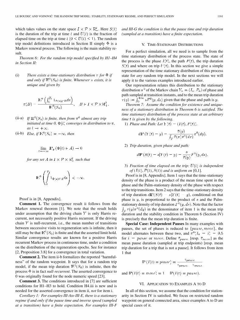
which takes values on the state space . Hereis the duration of the trip at time and is the fraction ofelapsed time on the trip at time . The randomtrip model definitions introduced in Section II simply is aMarkov renewal process. The following is the main stability re-sult.
Theorem 6: For the random trip model specified by H1–H4in Section II:
(i) There exists a time-stationary distribution for ifand only if is finite. Whenever exists, it isunique and given by
(ii-a) If is finite, then from almost any tripinitiated at time 0, converges in distribution to ,as .
(ii-b) Else, if , then
for any set in such that
Proof is in [8, Appendix].Comment 1. The convergence result ii follows from the
Markov renewal theorem [1]. We note that the result holdsunder assumption that the driving chain is only Harris re-current, not necessarily positive Harris recurrent. If the drivingchain is null-recurrent, i.e., the mean number of transitionsbetween successive visits to regeneration sets is infinite, then itstill may be that is finite and that the asserted limit hold.Similar convergence results are known for a positive Harrisrecurrent Markov process in continuous time, under a conditionon the distribution of the regeneration epochs. See for instance[2, Proposition 3.8] for a convergence in total variation.
Comment 2. The item ii-b formalizes the reported “harmful-ness” of the random waypoint. It says that for a random tripmodel, if the mean trip duration is infinite, then theprocess is in fact null-recurrent. The asserted convergence to0 was originally found for the node numeric speed [23].
Comment 3. The conditions introduced in [7] are sufficientconditions for H1–H3 to hold. Condition H4.iii is new and isneeded for the asserted convergence in item ii, not for item i.
Corollary 1: For examples III-Ato III-E, there is a stationaryregime if and only if the pause time and inverse speed (sampledat a transition) have a finite expectation. For examples III-F
and III-G the condition is that the pause time and trip duration(sampled at a transition) have a finite expectation.
V. TIME-STATIONARY DISTRIBUTIONS
For a perfect simulation, all we need is to sample from thetime stationary distribution of the process state. The state ofthe process is the phase , the path , the trip duration
and where on trip . In this section we give a simplerepresentation of the time stationary distribution of this processstate for any random trip model. In the next sections we willapply it to the various examples introduced earlier.
Our representation relates this distribution to the stationarydistribution of the Markov chain of phase andpath sampled at transition instants, and to the mean trip duration
given that the phase and path is .Theorem 7: Assume the condition for existence and unique-
ness of a stationary distribution in Theorem 6 is satisfied. Thetime stationary distribution of the process state at an arbitrarytime is given by the following.
1) Phase and Path: Let .
2) Trip duration, given phase and path:
3) Fraction of time elapsed on the trip: is independentof and is uniform on [0,1].
Proof is in [8, Appendix]. Item 1 says that the time-stationarydensity of the phase is a product of the mean time spent in thephase and the Palm-stationary density of the phase with respectto the trip transitions. Item 2 says that the time-stationary densityof trip duration , conditional on thatphase is , is proportional to the product of and the Palm-stationary density of trip duration . Note that the factor
in the denominator of item 1 is the mean tripduration and the stability condition in Theorem 6 (Section IV)is precisely that the mean trip duration is finite.
Special Case: Independent Pauses In many examples withpauses, the set of phases is reduced to , themodel alternates between these two, andfor or . Define [resp. ] as themean pause duration (sampled at trip endpoints) [resp. meantrip duration for a trip that is not a pause]. It follows from item1 that
and .
VI. APPLICATION TO EXAMPLES A TO D
In all of this section, we assume that the condition for station-arity in Section IV is satisfied. We focus on restricted randomwaypoint on general connected area, since examples A to D arespecial cases of it.
1162 IEEE/ACM TRANSACTIONS ON NETWORKING, VOL. 14, NO. 6, DECEMBER 2006
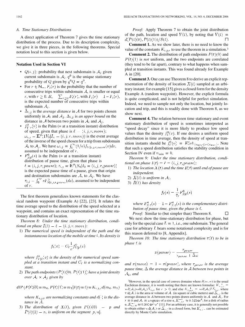
A. Time Stationary Distributions
A direct application of Theorem 7 gives the time stationarydistribution of the process. Due to its description complexity,we give it in three pieces, in the following theorems. Specialnotation local to this section is given below.
Notation Used in Section VI
• : probability that next subdomain is givencurrent subdomain is . is the unique stationaryprobability of given by .
• For , is the probability that the number ofconsecutive trips within subdomain is smaller or equal, with . , with ,
is the expected number of consecutive trips withinsubdomain .
• is the average distance in for two points chosenuniformly in and . is an upper bound on thedistance in between two points in and .
• is the Palm (= at a transition instant) distributionof speed, given that phase is ;
is the event averageof the inverse of the speed chosen for a trip from subdomain
to . We have ,assumed to be independent of .
• is the Palm (= at a transition instant)distribution of pause time, given that phase is
;is the expected pause time of a pause, given that originand destination subdomains are to . We have
, assumed to be independentof .
The first theorem generalizes known statements for the clas-sical random waypoint (Example A) [22], [23]. It relates thetime average speed to the distribution of the speed selected at awaypoint, and contains an exact representation of the time sta-tionary distribution of location.
Theorem 8: Under the time stationary distribution, condi-tional on phase :
1) The numerical speed is independent of the path and theinstantaneous location of the mobile at time . Its density is
where is the density of the numerical speed sam-pled at a transition instant and is a normalizing con-stant.
2) The path endpoints have a joint densityover given by
where are normalizing constants and is the dis-tance in .
3) The distribution of , given and, is uniform on the segment .
Proof: Apply Theorem 7 to obtain the joint distributionof the path, location and speed , by noting that
.Comment 1. As we show later, there is no need to know the
value of the constants to use the theorem in a simulation.3
Comment 2. The distribution of path endpoints andis not uniform, and the two endpoints are correlated
(they tend to be far apart), contrary to what happens when sam-pled at transition instants. This was found already for ExampleA in [20].
Comment 3. One can use Theorem 8 to derive an explicit rep-resentation of the density of location sampled at an arbi-trary instant; for example [15] gives a closed form for the densityExample A (random waypoint). However, the explicit formulais quite complicated, and is not helpful for perfect simulation.Indeed, we need to sample not only the location, but jointly lo-cation and trip, and this is readily done with Theorem 8, as weshow next.
Comment 4. The relation between time stationary and eventstationary distribution of speed is sometimes interpreted as“speed decay” since it is more likely to produce low speedvalues than the density . If one desires a uniform speeddistribution in time average, then the density of speed at tran-sition instants should be . Notethat such a speed distribution satisfies the stability condition inSection IV even if .
Theorem 9: Under the time stationary distribution, condi-tional on phase :
1) The location and the time until end of pause areindependent.
2) is uniform in .3) has density
where is the complementary distri-bution of pause time, given the phase is .Proof: Similar to (but simpler than) Theorem 8.
We next show the time-stationary distribution for phase, butonly for the special case , i.e., one subdomain. The generalcase for arbitrary bears some notational complexity and is forthis reason deferred to [8, Appendix].
Theorem 10: The time stationary distribution to be inphase is
and , where is the averagepause time, the average distance in between two points in
, and
3However, in the special case of convex domains where d(m;n) is the usualEuclidean distance, it is worth noting that there are known formulae: K =vol(A )vol(A ) �� , for r > 0, and else K = vol(A ) �� , wherevol(A ) is the area or volume ofA (in square or cubic meters) and �� is theaverage distance in A between two points drawn uniformly inA and A . Forr = 0 andA = a square of a size a, K � 0:5214a ; for a disk of radiusa,K � 0:9054� a [11]. For an arbitrary case, it is generally not possibleto obtain either vol(A ) or �� in a closed form, but K can be estimateddirectly by Monte Carlo simulation.
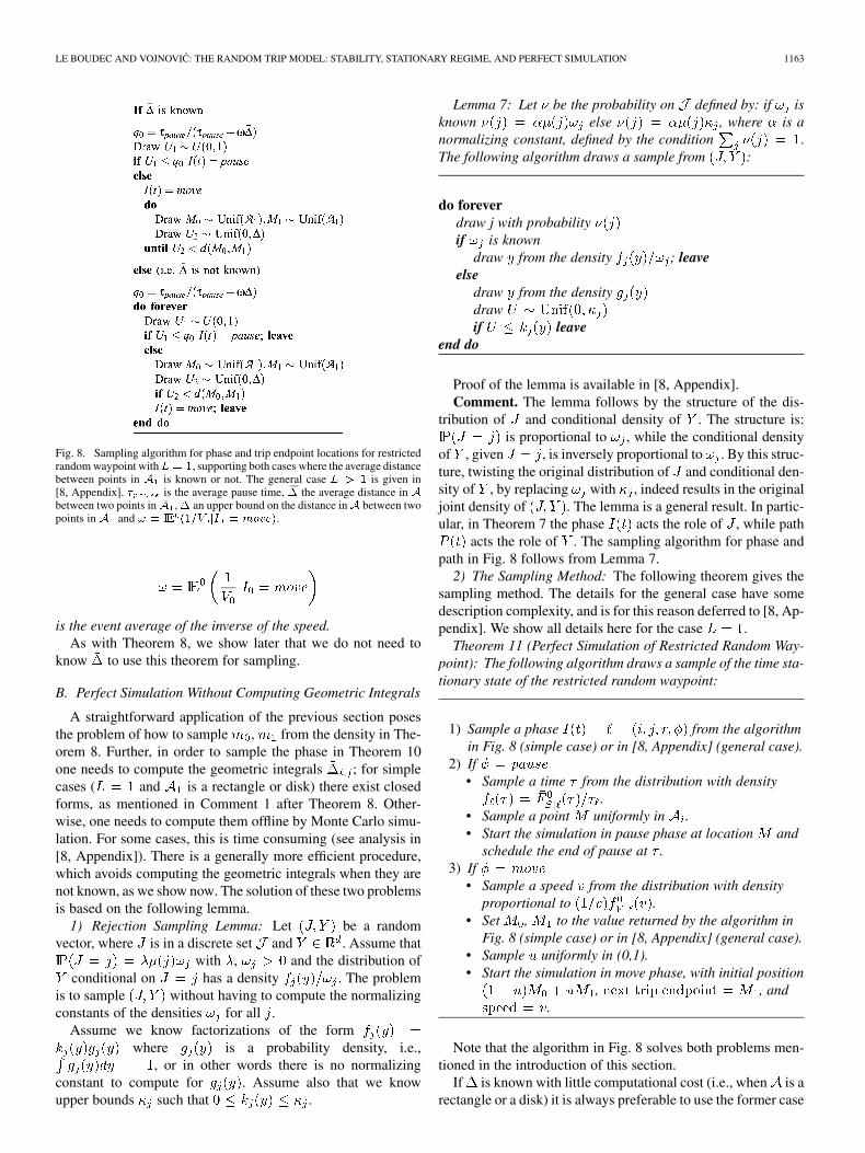
LE BOUDEC AND VOJNOVIC: THE RANDOM TRIP MODEL: STABILITY, STATIONARY REGIME, AND PERFECT SIMULATION 1163
Fig. 8. Sampling algorithm for phase and trip endpoint locations for restrictedrandom waypoint withL = 1, supporting both cases where the average distancebetween points in A is known or not. The general case L > 1 is given in[8, Appendix]. � is the average pause time, �� the average distance in Abetween two points inA , � an upper bound on the distance inA between twopoints in A and ! = IE (1=V jI = move).
is the event average of the inverse of the speed.As with Theorem 8, we show later that we do not need to
know to use this theorem for sampling.
B. Perfect Simulation Without Computing Geometric Integrals
A straightforward application of the previous section posesthe problem of how to sample , from the density in The-orem 8. Further, in order to sample the phase in Theorem 10one needs to compute the geometric integrals ; for simplecases ( and is a rectangle or disk) there exist closedforms, as mentioned in Comment 1 after Theorem 8. Other-wise, one needs to compute them offline by Monte Carlo simu-lation. For some cases, this is time consuming (see analysis in[8, Appendix]). There is a generally more efficient procedure,which avoids computing the geometric integrals when they arenot known, as we show now. The solution of these two problemsis based on the following lemma.
1) Rejection Sampling Lemma: Let be a randomvector, where is in a discrete set and . Assume that
with , and the distribution ofconditional on has a density . The problem
is to sample without having to compute the normalizingconstants of the densities for all .
Assume we know factorizations of the formwhere is a probability density, i.e.,
, or in other words there is no normalizingconstant to compute for . Assume also that we knowupper bounds such that .
Lemma 7: Let be the probability on defined by: if isknown else , where is anormalizing constant, defined by the condition .The following algorithm draws a sample from :
do foreverdraw j with probabilityif is known
draw from the density ; leaveelse
draw from the densitydrawif leave
end do
Proof of the lemma is available in [8, Appendix].Comment. The lemma follows by the structure of the dis-
tribution of and conditional density of . The structure is:is proportional to , while the conditional density
of , given , is inversely proportional to . By this struc-ture, twisting the original distribution of and conditional den-sity of , by replacing with , indeed results in the originaljoint density of . The lemma is a general result. In partic-ular, in Theorem 7 the phase acts the role of , while path
acts the role of . The sampling algorithm for phase andpath in Fig. 8 follows from Lemma 7.
2) The Sampling Method: The following theorem gives thesampling method. The details for the general case have somedescription complexity, and is for this reason deferred to [8, Ap-pendix]. We show all details here for the case .
Theorem 11 (Perfect Simulation of Restricted Random Way-point): The following algorithm draws a sample of the time sta-tionary state of the restricted random waypoint:
1) Sample a phase from the algorithmin Fig. 8 (simple case) or in [8, Appendix] (general case).
2) If• Sample a time from the distribution with density
.• Sample a point uniformly in .• Start the simulation in pause phase at location and
schedule the end of pause at .3) If
• Sample a speed from the distribution with densityproportional to .
• Set , to the value returned by the algorithm inFig. 8 (simple case) or in [8, Appendix] (general case).
• Sample uniformly in (0,1).• Start the simulation in move phase, with initial position
, , and.
Note that the algorithm in Fig. 8 solves both problems men-tioned in the introduction of this section.
If is known with little computational cost (i.e., when is arectangle or a disk) it is always preferable to use the former case
1164 IEEE/ACM TRANSACTIONS ON NETWORKING, VOL. 14, NO. 6, DECEMBER 2006
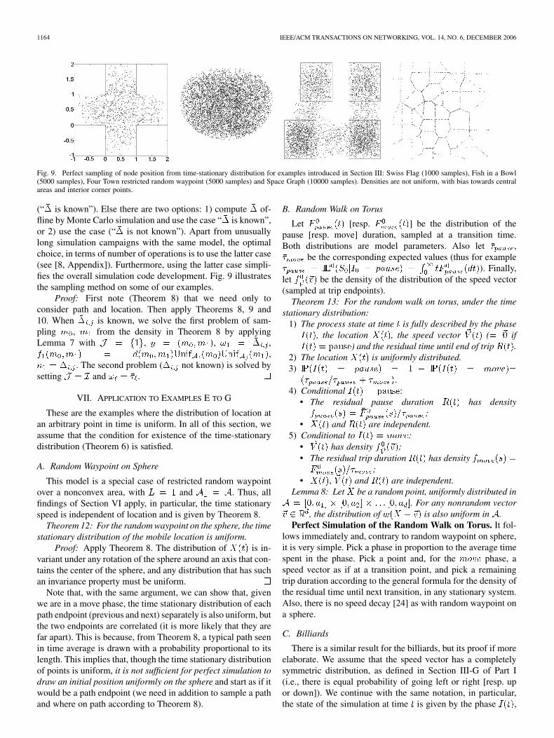
Fig. 9. Perfect sampling of node position from time-stationary distribution for examples introduced in Section III: Swiss Flag (1000 samples), Fish in a Bowl(5000 samples), Four Town restricted random waypoint (5000 samples) and Space Graph (10000 samples). Densities are not uniform, with bias towards centralareas and interior corner points.
(“ is known”). Else there are two options: 1) compute of-fline by Monte Carlo simulation and use the case “ is known”,or 2) use the case (“ is not known”). Apart from unusuallylong simulation campaigns with the same model, the optimalchoice, in terms of number of operations is to use the latter case(see [8, Appendix]). Furthermore, using the latter case simpli-fies the overall simulation code development. Fig. 9 illustratesthe sampling method on some of our examples.
Proof: First note (Theorem 8) that we need only toconsider path and location. Then apply Theorems 8, 9 and10. When is known, we solve the first problem of sam-pling , from the density in Theorem 8 by applyingLemma 7 with , , ,
,. The second problem ( not known) is solved by
setting and .
VII. APPLICATION TO EXAMPLES E TO G
These are the examples where the distribution of location atan arbitrary point in time is uniform. In all of this section, weassume that the condition for existence of the time-stationarydistribution (Theorem 6) is satisfied.
A. Random Waypoint on Sphere
This model is a special case of restricted random waypointover a nonconvex area, with and . Thus, allfindings of Section VI apply, in particular, the time stationaryspeed is independent of location and is given by Theorem 8.
Theorem 12: For the random waypoint on the sphere, the timestationary distribution of the mobile location is uniform.
Proof: Apply Theorem 8. The distribution of is in-variant under any rotation of the sphere around an axis that con-tains the center of the sphere, and any distribution that has suchan invariance property must be uniform.
Note that, with the same argument, we can show that, givenwe are in a move phase, the time stationary distribution of eachpath endpoint (previous and next) separately is also uniform, butthe two endpoints are correlated (it is more likely that they arefar apart). This is because, from Theorem 8, a typical path seenin time average is drawn with a probability proportional to itslength. This implies that, though the time stationary distributionof points is uniform, it is not sufficient for perfect simulation todraw an initial position uniformly on the sphere and start as if itwould be a path endpoint (we need in addition to sample a pathand where on path according to Theorem 8).
B. Random Walk on Torus
Let [resp. ] be the distribution of thepause [resp. move] duration, sampled at a transition time.Both distributions are model parameters. Also let ,
be the corresponding expected values (thus for example). Finally,
let be the density of the distribution of the speed vector(sampled at trip endpoints).
Theorem 13: For the random walk on torus, under the timestationary distribution:
1) The process state at time is fully described by the phase, the location , the speed vector ( if
) and the residual time until end of trip .2) The location is uniformly distributed.3)
.4) Conditional :
• The residual pause duration has density;
• and are independent.5) Conditional to :
• has density ;• The residual trip duration has density
;• , and are independent.
Lemma 8: Let be a random point, uniformly distributed in. For any nonrandom vector
, the distribution of is also uniform in .Perfect Simulation of the Random Walk on Torus. It fol-
lows immediately and, contrary to random waypoint on sphere,it is very simple. Pick a phase in proportion to the average timespent in the phase. Pick a point and, for the phase, aspeed vector as if at a transition point, and pick a remainingtrip duration according to the general formula for the density ofthe residual time until next transition, in any stationary system.Also, there is no speed decay [24] as with random waypoint ona sphere.
C. Billiards
There is a similar result for the billiards, but its proof if moreelaborate. We assume that the speed vector has a completelysymmetric distribution, as defined in Section III-G of Part I(i.e., there is equal probability of going left or right [resp. upor down]). We continue with the same notation, in particular,the state of the simulation at time is given by the phase ,
LE BOUDEC AND VOJNOVIC: THE RANDOM TRIP MODEL: STABILITY, STATIONARY REGIME, AND PERFECT SIMULATION 1165
the location , the speed vector ( if )and the residual time until end of trip .
Note that now there is a difference. The instant speedis, in general, not constant during an entire trip and may differfrom the unreflected speed chosen at the beginning of thetrip (as it gets reflected at the boundary of ). Let bethe density of the distribution of the nonreflected speed vector(sampled at trip endpoints).
Theorem 14: For the random walk with reflection, the sameholds as in Theorem 13 after replacing the first bullet of item 5by
• has density .The following lemma is used in the proof of Theorem 14; it
says that, at the end of a trip that starts from a uniform pointand a completely symmetric initial speed vector , the reflecteddestination point and speed vector are independent andhave same distribution as initially.
Lemma 9: Let be a random point, uniformly distributed in. Let be a random vector in independent of and with
completely symmetric distribution. Let be a constant.Define and .
has the same joint distribution as .Remark: It is important to use the instant speed vector
and not the unreflected speed vector when describing thesimulation state: indeed the description by phase , location
, unreflected speed vector ( if ) andresidual time until end of trip is not sufficient to continuethe simulation (one needs to remember which reflection wasapplied to the speed vector) and is thus not Markov.
Also note that, in time stationary averages, the locationand the unreflected speed vector are not independent. Forexample, given that the unreflected speed vector is
and the trip duration is , it is more likelythat is in the second right half of the rectangle. In con-trast, and the instant speed vector are independent,as shown by the theorem.
Perfect Simulation of the Billiards. It is similar to therandom walk on torus.
VIII. RELATED WORK
For a survey of existing mobility models, see the work byCamp, Boleng, and Davies [10] and the references therein.Bettstetter, Harnstein, and Pérez-Costa [11] studied thetime-stationary distribution of a node location for classicalrandom-waypoint model. They observed that the time-sta-tionary node location is nonuniform and it has more mass inthe center of a rectangle. A similar problem has been furtherstudied by Bettstetter, Resta, and Santi [5]. A closed-formexpression for the time-stationary density of a node locationis obtained only for random-waypoint on a one-dimensionalinterval; for two dimensions only approximations are obtained.Note that in Theorem 8, we do have an exact representation ofthe distribution of node location as a marginal of a distributionwith a known density. Neither [11] nor [5] consider how to runperfect simulations.
It is the original finding of Yoon, Liu, and Noble [23] thatthe default setting of the classical random-waypoint exhibits
speed decay with time. The default random-waypoint assumesthe event-stationary distribution of the speed to be uniform onan interval . The authors found that if a node is initial-ized such that origin is a waypoint, the expected speed decreaseswith time to 0. This in fact is fully explained by the infinite ex-pected trip duration as sampled at trip transitions, which im-plies the random process of mobility state is null-recurrent; seeSection IV. In a subsequent work [24], the same authors advo-cate to run “sound” mobility models by initializing a simulationby drawing a sample of the speed from its time-stationary dis-tribution. We remark that this is only a partial solution as speedis only a component of node mobility state. For this reason, theauthors in [24] do not completely solve the problem of perfectsimulation. Another related work is that of Lin, Noubir, and Ra-jaraman [16] that studies a class of mobility models where traveldistance and travel speed between transition points can be mod-eled as a renewal process. The renewal assumption was alsomade in [23] and [24]. We note that this assumption is not veri-fied with mobility models such as classical random-waypoint onany nonisotropic domain, such as a rectangle, for example. Therenewal assumption has been made to make use of a “cycle” for-mula from the theory of renewal random processes. From Palmcalculus, we know that the “cycle” formula is in fact Palm inver-sion formula, which we used extensively throughout the paper,and that applies more generally to stationary random processes;this renders the renewal assumption unnecessary.
Perhaps the work closest to ours is that of Navidi, Camp, andBauer in [20] and [22]. As discussed in Section I-D, we providea systematic framework that allows to formally prove some ofthe implicit statements in [20] and generalize to a broader class.Further, our perfect sampling algorithm differs in that it workseven when geometric constants are not a priori known. In [19],Nain, Towsley, Liu, and Liu consider the random walk on torusand billiards models (which they call “random direction”), as-suming the speed vectors are isotropic. They find that the sta-tionary regime has uniform distribution, and advocate that thisprovides an interesting bias-free model.
There are other well-established techniques for performingperfect simulation. The method in [21] applies to a large class ofMarkov chains on which some partial ordering can be defined,and uses coupling from the past (sample trajectories starting inthe past at different initial conditions). The technique presentedin this paper is much simpler, as, unlike in the case of [21], wecan obtain an explicit representation of the stationary distribu-tion.
IX. CONCLUSION
The random trip model provides a framework to analyze andsimulate stable mobility models that are guaranteed to havea unique time-stationary distribution. Moreover, conditionsare provided that guarantee convergence in distribution to atime-stationary distribution, from origin of an arbitrary trip.It is showed that many known random mobility models arerandom trip models.
For stable random trip models, if the initial node mobilitystate is not sampled from the time-stationary distribution, thenode mobility state distribution converges to the time-stationary
1166 IEEE/ACM TRANSACTIONS ON NETWORKING, VOL. 14, NO. 6, DECEMBER 2006
distribution. The rate of this convergence depends on the geom-etry of the mobility domain and specifics of the trip selection.In order to alleviate this initial transience altogether, we providea perfect sampling algorithm to initialize node mobility state toa sample from the time-stationary distribution, so that a nodemovement is a time-stationary realization.
The web page “random trip model” at http://ica1wwww.epfl.ch/RandomTrip provides a repository of random tripmodels and a free to download perfect sampling software touse for simulations.
ACKNOWLEDGMENT
The perfect sampling ns-2 code pointed out in this paper wasimplemented by S. PalChaudhuri. M. Vojnovic is grateful to S.Capkun for referring him to the mobility problem studied in thispaper.
REFERENCES
[1] G. Alsmeyer, “The Markov renewal theorem and related results,”Markov Proc. Rel. Fields, vol. 3, pp. 103–127, 1997.
[2] S. Asmussen, Applied Probability and Queues, 2nd ed. New York:Springer, 2003.
[3] F. Baccelli and P. Brémaud, Elements of Queueing Theory: PalmMartingale Calculus and Stochastic Recurrences, 2nd ed. Berlin:Springer-Verlag, 2003, vol. 26, Applications of Mathematics.
[4] C. Bettstetter, “Mobility modeling in wireless networks: categoriza-tion, smooth movement, and border effects,” Mobile Comput. Commun.Rev., vol. 5, no. 3, pp. 55–67, 2001.
[5] ——, “The node distribution of the random waypoint mobility modelfor wireless ad hoc networks,” IEEE Trans. Mobile Comput., vol. 2, no.3, pp. 257–269, Jul.–Sep. 2003.
[6] L. Blazevic, J.-Y. Le Boudec, and S. Giordano, “A location-basedrouting method for mobile ad hoc networks,” IEEE Trans. MobileComput., vol. 3, no. 4, pp. 97–110, Dec. 2004.
[7] J.-Y. Le Boudec and M. Vojnovic, “Perfect simulation and stationarityof a class of mobility models,” in Proc. IEEE INFOCOM 2005, Miami,FL, Mar. 2005, pp. 2743–2754.
[8] ——, “The Random Trip model: Stability, stationary regime, andperfect simulation,” Microsoft Research, Cambridge, U.K., Tech.Rep. MSR-TR-2006-26, 2006 [Online]. Available: http://research.mi-crosoft.com/research/pubs/view.aspx?type=Technical%20Report&id=1070
[9] J. Broch, D. A. Maltz, D. B. Johnson, Y.-C. Hu, and J. Jetcheva, “Aperformance comparison of multi-hop wireless ad hoc network routingprotocols,” Mobile Comput. Netw., pp. 85–97, 1998.
[10] T. Camp, J. Boleng, and V. Davies, “A survey of mobility models for adhoc network research,” WCMC: Special Issue on Mobile Ad Hoc Net-working: Research, Trends and Applications, vol. 2, no. 5, pp. 483–502,2002.
[11] H. Hartenstein, C. Bettstetter, and X. Pérez-Costa, “Stochastic prop-erties of the random waypoint mobility model,” ACM/Kluwer WirelessNetworks, Special Issue on Modeling and Analysis of Mobile Networks,vol. 10, no. 5, pp. 555–567, Sep. 2004.
[12] G. Hardy, J. E. Littlewood, and G. Pólya, Inequalities, 2nd ed. Cam-bridge, U.K.: Cambridge Univ. Press, 1952.
[13] A. Jardosh, E. M. Belding-Royer, K. C. Almeroth, and S. Suri, “To-wards realistic mobility models for mobile ad hoc networking,” in Proc.ACM MOBICOM 2003, San Diego, CA, 2003, pp. 217–229.
[14] J.-Y. Le Boudec, “On the stationary distribution of speed and locationof random waypoint,” IEEE Trans. Mobile Comput., vol. 4, no. 4, pp.404–405, Jul.-Aug. 2005.
[15] ——, “Understanding the simulation of mobility models with palmcalculus,” Perform. Eval., in press, also available as EPFL Tech. Rep.EPFL/IC/2004/53.
[16] G. Lin, G. Noubir, and R. Rajamaran, “Mobility models for ad hocnetwork simulation,” in Proc. IEEE INFOCOM 2004, Hong Kong, Apr.2004, pp. 454–463.
[17] T. Lindvall, Lectures on the Coupling Method. New York: Dover,2002, originally published by Wiley in 1992.
[18] M. Drmota and R. F. Tichy, Sequences, Discrepancies and Applica-tions. New York: Springer, 1997, vol. 1651, Lecture Notes in Math-ematics.
[19] P. Nain, D. Towsley, B. Liu, and Z. Liu, “Properties of random directionmodels,” in Proc. IEEE INFOCOM 2005, Miami, FL, Mar. 2005, pp.1897–1907.
[20] W. Navidi and T. Camp, “Stationary distributions for the random way-point mobility model,” IEEE Trans. Mobile Comput., vol. 3, no. 1, pp.99–108, Jan.-Feb. 2004.
[21] J. G. Propp and D. B. Wilson, “Exact sampling with coupled Markovchains and applications to statistical mechanics,” Random Struct.Algor., vol. 9, no. 1–2, pp. 223–252, 1996.
[22] T. Camp, W. Navidi, and N. Bauer, “Improving the accuracy of randomwaypoint simulations through steady-state initialization,” in Proc. 15thInt. Conf. Modeling and Simulation (MS’04), Marina del Rey, CA, Mar.2004, pp. 319–326.
[23] J. Yoon, M. Liu, and B. Noble, “Random waypoint consideredharmful,” in Proc. IEEE INFOCOM 2003, San Francisco, CA, pp.1312–1321.
[24] ——, “Sound mobility models,” in Proc. ACM MOBICOM 2003, SanDiego, CA, pp. 205–216.
Jean-Yves Le Boudec (M’89–SM’01–F’05) gradu-ated from Ecole Normale Superieure de Saint-Cloud,Paris, France, where he received the Agregation inmathematics in 1980 (rank 4), and received the doc-torate from the University of Rennes, France, in 1984.
He is a full Professor at EPFL and Director of theInstitute of Communication Systems. From 1984 to1987, he was with INSA/IRISA, Rennes. In 1987,he joined Bell Northern Research, Ottawa, Canada,as a Member of Scientific Staff in the Network andProduct Traffic Design Department. In 1988, he
joined the IBM Zurich Research Laboratory where he was Manager of theCustomer Premises Network Department. In 1994, he joined EPFL as anAssociate Professor. His interests are in the performance and architecture ofcommunication systems. In 1984, he developed analytical models of multipro-cessors and multiple bus computers. In 1990, he invented the concept called“MAC emulation” which later became the ATM forum LAN emulation project,and developed the first ATM control point based on OSPF. He also launchedpublic domain software for the interworking of ATM and TCP/IP under Linux.He proposed in 1998 the first solution to the failure propagation that arises fromcommon infrastructures in the Internet. He contributed to network calculus,a recent set of developments that forms a foundation to many traffic controlconcepts in the internet, and co-authored a book on this topic.
Dr. Le Boudec received the IEEE INFOCOM 2005 Best Paper Award (withMilan Vojnovic of Microsoft Research) for elucidating the perfect simulationand stationarity of mobility models. He has been on the program committee ofmany conferences, including SIGCOMM, SIGMETRICS and INFOCOM, wasmanaging editor of the journal Performance Evaluation from 1990 to 1994, andis on the editorial board of the IEEE/ACM TRANSACTIONS ON NETWORKING.
Milan Vojnovic (M’04) received the M.Sc. and B.Sc.degrees in electrical engineering from the Universityof Split, Croatia, in 1998 and 1995, respectively, andthe Ph.D. degree in technical sciences from EPFL,Lausanne, Switzerland, in 2003.
He is a Researcher with the Systems and Net-working Group at Microsoft Research, Cambridge,U.K. His research interests are in architecture andperformance of computer systems with particularinterests in mobile systems, information dissemi-nation, and usage control of network resources. He
undertook an internship with the Math Center of Bell Laboratories, MurrayHill, NJ, in 2001.
Dr. Vojnovic received the ACM SIGMETRICS 2005 Best Paper Award (withLaurent Massoulié) for a work on performance of file swarming systems, theIEEE INFOCOM 2005 Best Paper Award (with Jean-Yves Le Boudec) for awork on stationarity and perfect simulation of random mobility models, and theITC-17 2001 Best Student Paper Award (with Jean-Yves Le Boudec) for a workon TCP-friendliness of equation-based congestion control. In 2005, he receivedthe ERCIM Cor Baayen Award.


![[a. M. Yaglom] an Introduction to the Theory of Stationary Random functions](https://img.pdfslide.net/doc/110x75/552c10d74a7959f57c8b464d/a-m-yaglom-an-introduction-to-the-theory-of-stationary-random-functions.jpg)