The Relationship between Government Revenue and …hrmars.com/hrmars_papers/The_Relationship_between_Government... · The Relationship between Government Revenue ... The relationship

International Journal of Academic Research in Business and Social Sciences March 2014, Vol. 4, No. 3

ISSN: 2222-6990

171 IJARBSS – Impact Factor: 0.305 (Allocated by Global Impact Factor, Australia) www.hrmars.com

The Relationship between Government Revenue and Government Expenditure in Iran

Mohsen Mehrara Faculty of Economics, University of Tehran, Iran

Email: [email protected]

Abbas ali Rezaei

M.S in Economics, Organization of Finance and Economic Affairs in Sistan & Balouchestan Email: [email protected]

DOI: 10.6007/IJARBSS/v4-i3/687 URL: http://dx.doi.org/10.6007/IJARBSS/v4-i3/687

Abstract The relationship between government revenue and government expenditure has been an important topic in public economics, given its relevance for policy especially with respect to the budget deficit. Besides the theoretical arguments about this relation, vast empirical literature is also available all over the world. The purpose of this paper is to investigate the relationship between government revenue and government expenditure in IRAN by using annual data and applying the Toda - Yamamoto Granger causality test for the period of 1978 to 2011. it is an important issue for this country but scare empirical literature available on this issue for IRAN. The research uses the annual time series data which is obtained from the website of Central Bank. Data properties were analyzed to determine their stationary using unit root tests ADF and Zivot-Andrews unit root test which indicated that the series are I(1). The Toda - Yamamoto Granger causality test found unidirectional causality running from government revenue to government expenditure. So, these results consistent with the revenue-spend hypothesis. Our results support the Freidman (1978) and Buchanan-Wagner hypothesis that government revenues cause expenditure. Keywords: granger causality, government revenue, government expenditure, Toda-Yamamoto approach. JEL Classification: H2, H5, H62, O17

1. Introduction To take a good decision and to improve their societies, the governments need to design the budget. To do its functions a government uses budget as a planning and financial tool. One of the debates of public finance is to find the relationship between government revenue and expenditure and considerable theoretical and empirical research has been carried out on this issue. If policymakers understand the relationship between government expenditure and government revenue, without a pause government deficits can be prevented. Hence the


ISSN: 2222-6990


relationship between government expenditure and government revenue has attracted significant interest. This is due to the fact that the relationship between government revenue and expenditure has an impact on the budget deficit. Over the Past three decades, a large number of studies have investigated the relationship between government revenue and government expenditure. Understanding the relationship between government revenue and government expenditure is important from a policy point of view, especially for Asian countries, which is suffering from persistent budget deficits. There is a budget deficit while the government revenues are less than the government expenditures. Vice versa, when the government expenditures less than its revenues it is said that the government has budget surplus. There are always the budget deficit for iran during all of years of this study. In other words, the budget deficit is a characteristic of Iran economics .Some time the governments to reduce the unemployment rate at their societies use the budget deficit policy but having the budget deficit in the long period not only is a policy but also is a problem for society that it needs to solve. To solve this problem the government should reduce its expenditures or it should increase its revenues resources. The budget revenue resources should be stationary and they must have the lowest fluctuations. Strongly dependent budget with the oil revenue shows the government have to change its expenditures or revenues. To achieve these aims the government should know the relationship between government revenues and expenditures. It has been observed that in some cases revenue increase or expenditures reduction affect on its corresponding variable and makes the adopted policy ineffective. So before to make a decision about reducing of the expenditure or increasing revenues it is important to know the amount of dependences of those variables that affect on the government expenditures. To obtain the appropriate financial policy to reduce or remove budget deficit it is necessary to find the relationship between government revenues and expenditures. The main purpose of this paper is to investigate the relationship between government revenue and expenditure in Iran for the period from 1978-2011. The paper is divided into five sections. Following this introduction, literature review of relevant studies will be presented. Section three will discuss data and methodology that is used in this research. Empirical results are reported in section four. Section five will conclude this exercise.

2. Theoretical Literature Review: The causal relationship between revenues and government expenditure is a classic problem of Public Economics. There are four propositions that can potentially explain observed spending-revenue behavior. The propositions are briefly discussed as follows: Friedman leads the tax-and-spend school, which contends that raising taxes will simply lead to more spending. Friedman (1982) [cited in Narayan (2005: 1205)] puts his point in the following way: “You cannot reduce the deficit by raising taxes Increasing taxes only results in more spending, leaving the deficit at the highest level conceivably accepted by the public. Political rule number one is government spends what government receives plus as much more as it can get away with”. Also Milton Friedman (1982) suggests cutting taxes as a remedy to budget deficits, since taxes have a positive causal impact on government expenditure. According to Friedman, a cut in tax leads to higher deficits, which should influence government to reduce its level of spending, (Moalusi, 2004). Buchanan and Wagner (1977, 1978) put forward an alternative version of the tax-and-spend hypothesis. In contrast to Friedman (1978), they argue that tax increases would


ISSN: 2222-6990


lead to spending reductions. The building block of the Buchanan and Wagner (1977, 1978) version of the tax-and-spend hypothesis is that taxpayers suffer from fiscal illusion. According to the authors, tax cuts lower the perceived price of government provided goods and services by the public, which in turn boosts the public demand for these goods and services. However, the public may actually incur even higher costs. One reason for this is the indirect inflation taxation that results if the government resorts to excessive money creation. Another reason is higher interest rates associated with government debt financing may crowd out private investment. To reduce expenditures, Buchanan and Wagner favor limiting the ability of the government to resort to deficit financing. In sum, while tax changes as before drive spending changes, the relationship between the two is a negative one. The second school known as spend-and-tax school is built on the tenet that expenditure causes revenue proposed by Peacock and Wiseman (1961, 1979). According to the spend-and-tax hypothesis, the level of spending is first determined by the government and then tax policy and revenue are adjusted to accommodate the desired level of spending. A version of this hypothesis is suggested by Roberts (1978), and Peacock and Wiseman (1979) according to whom crisis situations (due to for example wars, natural disasters, or deep recessions) justify temporary increases in expenditures and taxes to pay for them. However, tax increases may become permanent; reflecting an upward adjustment in the level of tax tolerance of the citizens and their attitude towards the proper size of the government after the crisis has passed. This in turn allows for a permanent increase in the level of government expenditures. Another version of this hypothesis is based on the works of Barro (1974, 1979, 1986). In his tax smoothing hypothesis, government spending is considered as an exogenous variable to which taxes adjust. Moreover, the intertemporal budget constraint requires that an increase in current expenditures be matched by higher future taxes. Barro, therefore, rejects the notion that the taxpayers suffer from fiscal illusion. Quite the contrary, within the framework of the Ricardian equivalence theorem, he maintains that taxpayers are sophisticated, or rational, enough to see that an increase in the current debt in nothing but a delayed form of taxation. Taxpayers are, therefore, expected to fully capitalize the future tax liability. As pointed out by von Furstenberg et al. (1992), changes in spending can precede changes in taxes if a political majority raises pre-election expenditures, which are then paid for by subsequent post-election tax increases, or if they cut taxes as a compensation for earlier decisions to restrain expenditures. Since it is changes in expenditures that drive changes in taxes in this scenario, the preferred approach to fiscal deficit reduction relies on cutting expenditures. Fiscal synchronization hypothesis as the third school of thought argues that governments may change expenditure and taxes concurrently (Meltzer & Richard, 1981; Musgrave, 1966). This implies bidirectional causality between government expenditure and revenue. Under the fiscal synchronization hypothesis, citizens decide on the level of spending and taxes. This is done through comparing the benefits of government to citizen’s marginal cost, (Narayan, 2005). Barro’s (1979) tax smoothing model provided further credence to the fiscal synchronization hypothesis. His model was based on the Ricardian equivalence view that deficit financed government expenditure today results in future tax increases, (Narayan, 2005). The implication of this hypothesis is that causal relationship between government revenue and spending is bidirectional.


ISSN: 2222-6990


Finally, fourth school, fiscal neutrality school, proposed by Baghestani and McNown (1994) believe that none of the above hypotheses describes the relationship between government revenues and expenditure. Government expenditure and revenues are each determined by the long run economic growth reflecting the institutional separation between government revenues and expenditure that infers that revenue decisions are made independent are expenditure decisions. A major advocate of this view is Wildavsky (1988) who maintains that separate institutions such as the executive and legislative branches of the US government participate in the budgetary process to determine the level of taxation and spending. Budgeting can be incremental and adjustments can be made on the margin if these separate institutions reach a consensus on the fundamentals. In this case there is no causality between the two variables, and hence they are independent of one another.

3. Empirical Literature Review Numerous empirical studies available on revenue and expenditure nexus all over the world but there is no consensus about the linkage between these variables. Though over the last three decades several studies have been carried out in different countries to investigate the issue in the public economics, findings vary from country to country and also within the country. Considerable empirical works have been done with respect to the four above mentioned hypotheses. Using different econometric methods, studies have reached to different results. Different studies have focused on different countries, time periods, and have used different proxy variables for government revenue and expenditure. The empirical outcomes of these studies have been varied and sometimes conflicting. The results differ even on the direction of causality and it is long-term versus short term impact on government policy. We now move on to review some of the empirical studies of the relationship between government revenue and expenditure. Hasan and Lincoln (1997) carried out a research on this issue for United Kingdom by using cointegration technique and quarterly data from 1961-93 was used for this purpose. This study reveals that government tax revenue Granger causes government expenditures and vice versa. E.g. Shah and Baffes (1994) in their study for Latin American countries concluded bidirectional causality between government revenue and expenditure for Argentina over the 1913-1984 periods and for Mexico over the 1895-1984 periods; while for Brazil they found unidirectional causality running from revenue to expenditure. Owoye (1995) investigated the issue for the G7 countries. He found bidirectional causality for five of the seven countries and for Japan and Italy he found causality running from revenue to expenditure. Abdul Aziz and Shah Habibullah (2000) investigated causality between taxation and government spending by using an application of Toda-Yamamoto approach in Malaysia for the period 1960 to 1997. Their evidence generally supports the existence of bidirectional causality between government spending and tax revenues. Kollias and Makrydakis (2000) examined tax and spending relationship in four countries namely; Greece, Portugal, Spain, Ireland which are comparatively poorer countries in European Union. They found that cointegration prevails in only Greece and Ireland cases and whereas there is no long run relationship in the models for Spain and Portugal. Moreover, bidirectional causality between government spending and revenue exists in Greece and Ireland. As far as Spain and Portugal cases are concerned, in the former country, causality runs from revenue to expenditure and in the later country, there is no causal link between these two important fiscal variables. Chang et al (2002) conducted a study to examine


ISSN: 2222-6990


this relationship in ten industrialized countries including three newly industrialized Asian economies namely, Taiwan, South Korea and Thailand. In this study, GDP variable is also included in the model as a control variable along with government expenditures and tax variables and Johansen cointegration technique is exercised for analysis. They claimed that cointegration among the variables prevails for seven countries and found causality from government revenues to government expenditures for UK, USA, South Korea, Japan and Taiwan whereas causality runs from government expenditures to revenues for South Africa and Australia. This study also found independence between revenues and expenditures for New Zealand and Thailand. Maghyereh and Sweidan (2004) examined tax-spend, spend-tax and fiscal synchronization hypothesis for Jordan using annual time series data from 1969 to 2002. The authors used real GDP as control variable along with real government expenditures and real government revenues and Granger causality test based on Multivariate ECM. They conclude evidence in favor of bidirectional causality between revenue and expenditure. The result also suggests that there is long-run interdependence between output and fiscal variables indicating effectiveness of fiscal policy in Jordan. Carneiro et al. (2005) investigated this issue for Guinea-Bissau over the period 1981 to 2002. They found that Guinea-Bissau’s experience is consistent with the “spend - tax” hypothesis. Barua (2005) examined revenue and expenditure causality in Bangladesh by using annual data over the period 1974-2004. The results of Johansen test suggest that there is a long-run relationship between government expenditure, revenue and GDP and the Granger Causality test on the corresponding Vector Error Correction (VEC) model suggests that there is no causal relationship between revenue and expenditure in the short run. It is also observed that the short run relation extends from both the fiscal variables to GDP, and not the other way around. Tsen and Kian-Ping (2005) examined this relationship in Malaysia for the period from 1965 – 2002. Augmented Dickey-Fuller and Phillips-Perron Unit root tests, Johansen cointegration and error correction models were applied to data. The results supported tax-spend hypothesis. Government revenue was found to Granger cause expenditure in Malaysia. In another study, Narayan and Narayan (2006) found tax-and-spend hypothesis for Mauritius, El Salvador, Chile, Paraguay and Venezuela. For Haiti, there is evidence for supporting the fiscal synchronization hypothesis, while for Peru, South Africa, Guatemala, Guyana, Uruguay and Ecuador there is evidence of neutrality by application of the Toda and Yamamoto (1995) test for Granger causality. Nyamongo et al. (2007) in a study of the government revenue and expenditure nexus in South Africa found different results. A monthly data was used, and modified unit root test and Vector Error Correction Model (VECM) were applied on data. It was found that government revenue and expenditure are cointegrated, and a long-run relationship exists between them. Applying Granger causality through VECM model, it was found bidirectional Granger causality which supports fiscal synchronization hypothesis. In the short-run no Granger causality was found between variable, suggesting fiscal neutrality hypothesis in South Africa for the period of study. the study Wolde-Rufael (2008) for 13 African countries by using Toda and Yamamoto causality test show the direction of causation are mixed and his empirical evidence suggests that there was a bidirectional causality running between expenditure and revenue for Mauritius, Swaziland and Zimbabwe; no causality in any direction for Botswana, Burundi and Rwanda; unidirectional causality running from revenue to expenditure for Ethiopia, Ghana, Kenya, Nigeria, Mali and Zambia; and an un-directional causality running from expenditure to revenue for Burkina Faso only. Chaudhuri and Sengupta


ISSN: 2222-6990


(2009), by using an error-correction model and Granger causality test for southern states in India reported that the tax-spend hypothesis is supported by the analysis and also the spend-tax hypothesis is valid for some states. Ravin thirakumaran (2011) examined the relationship between government revenue and expenditure in Sri Lanka for the period from 1977-2009. A time series methodology of Engle-Granger’s approach of cointegration and error correction model framework is investigated. The study concluded that bidirectional causality exists between government revenue and expenditure and there is long-run equilibrium between the two variables in Sri Lanka economy. Subhani et al. (2012) found the opposite causality direction confirming the tax-spend hypothesis. They studied the causality direction between government expenditure and revenue for Pakistan. Annual data for the period from 1979-2010 were used, and Granger causality was applied to variables in question. The paper found that government revenue Granger cause government expenditure in Pakistan for the period under investigation. To the best of the author's knowledge ,The evidence on the relationship between government revenue and expenditure for Iran is scarce. Zonnoor, S. H (1995) examined the growth of government expenditures and revenues in Iran over the period of 1970 - 1990 in light of conventional theories as to the nature of public sector economic activity. In his study simple forms of government expenditure and tax functions are estimated. They also examined the speed of the adjustment process by estimating a simple disequilibrium model of government expenditures and receipts. Using a constant shares model as well as a constant marginal shares model, they compared the pattern of expenditures and the revenues structure before and after the Iran’s revolution.Elyasi and Rahimi (2012) found bidirectional causality between government revenue and expenditure in Iran. Annual data for the period from 1963-2007 were used, and variables were tested for stationarity. The paper included a comprehensive list of studies on causality between government revenue and expenditure for country specific and for multi-countries studies. The evidence cited on the direction of causality is mixed in those studies. Different data sets, econometric methodologies and different country characteristics are some of reasons cited for the different results on the direction of causality.

4. Toda-Yamamoto Augmented Granger Causality Approach Various tests are present to check the causality among variables i.e. Granger (1969), Engle & Granger (1987) and Johansen & Jesulious (1990). These tests are not free from errors like they require stationarity requirements, selection of maximum lag length and they are very sensitive to model specification. It is necessary to pretest the unit root and cointegration while applying these tests. To overcome these problems, the present study applies a more robust causality technique given by Toda Yamamoto (1995) and it is further explained by Rambaldi & Doran (1996) and Zapata & Rambaldi (1997).The Augmented Granger Causality Approach given by Toda Yamamoto (1995) is very simple to apply and it also follows asymptotic Chi-square distribution. The major advantage of above said approach is that, in this technique, it is not necessary to check the pre testing of the order of integration or cointegration properties among variables (Toda Yamamoto, 1995; Dolado & Lütkepohl, 1996; Giles & Mirza, 1999). Rambaldi & Doran (1996) have modified Wald test that is considered more efficient when Seemingly Unrelated Regression (SUR) Model is used in the estimation. One of the attractiveness of using SUR is that it takes care of possible simultaneity bias in the system of equations.


ISSN: 2222-6990


This test has an asymptotic chi-squared distribution with k degrees of freedom in the limit when a VAR[k+dmax] is estimated (where dmax is the maximal order of integration for the series in the system). Two steps are involved with implementing the procedure. The first step includes determination of the lag length (k) and the maximum order of integration (dmax) of the variables in the system. Measures such the Akaike Information Criterion (AIC), Schwarz Information Criterion (SC), Final Prediction Error (FPE) and Hannan-Quinn (HQ) Information Criterion can be used to determine the appropriate lag order of the VAR. , we use Akaike Information Criterion (AIC) and Schwarz Information Criterion (SC) to select the optimal lag to include in models. We use the Augmented Dickey-Fuller tests to determine the maximum order of integration. Given the VAR(k) selected, and the order of integration dmax is determined, a levels VAR can then be estimated with a total of p=[k+ dmax] lags. The second step is to apply standard Wald tests to the first k VAR coefficient matrix (but not all lagged coefficients) to conduct inference on Granger causality. Also ,Toda and Yamamoto cannot be used if the maximum number of unit-roots in the VAR is larger than the optimal lag-length. Thus, in some cases, it might not be possible to conduct causality tests.

4-1. DATA AND ECONOMETRIC METHODOLOGY This study aims to provide empirical evidence on the relationship between government revenue and expenditure for Iran and give insights on the causality patterns. Therefore, in this paper the Toda-Yamamoto approach is used to check the causality between two variable. However before going to estimate the data it is necessary to check the unit root presence in the data and for that in this study the ADF and Zivot-Andrews unit root test is used in order to know the order of integration of the series. Although, to determine lag length of model , we employee Final prediction error (FPE), Akaike information criterion (AIC) and Schwarz information criterion (SC). Annual time series variables data which utilized in this paper are include the government revenue (TR) and government expenditure (GE) gathered from web site Central Bank of Iran. The logarithm of the government expenditures and government revenues are used in the empirical analysis. The transformation of the series to logarithms is intended to eliminate the problem of heteroskedasticity. Annual data for the period from 1978 – 2011 are used in this study. We select these period because time series data on government revenue and government expenditure are only available for this period.

4-2. Findings and Discussion 4-2-1. Augmented Dickey-Fuller and Zivot and Andrews Unit Root Testing for order of integration: Most of time series have unit root as many studies indicated including (Nelson and Polsser, 1982), and as proved by (Stock and Watson, 1988) and (Campbell and Perron, 1991) among others that most of the time series are non-stationary. The presence of a unit root in any time


ISSN: 2222-6990


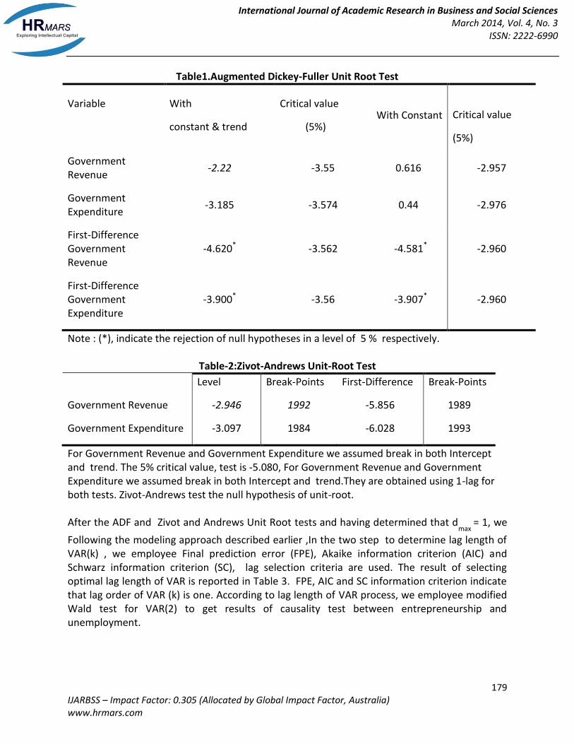
series means that the mean and variance are not independent of time. Conventional regression techniques based on non stationary time series produce spurious regression and statistics may simply indicate only correlated trends rather than a true relationship (Granger and Newbold, 1974). Conventional tests for identifying the existence of unit roots in a data series include that of the Augmented Dickey Fuller (ADF) (1979, 1981) . Our main reason for conducting unit root tests is to determine the extra lags to be added to the vector autoregressive (VAR) model for the Toda and Yamamoto test. Prior to testing for a causality relationship between the time series, it is necessary to establish whether they are integrated of the same order. To this end in the first step of the empirical analysis, the Augmented Dickey Fuller (ADF) unit-root tests have been carried out for the both variables: government expenditure and Government Revenue, both in logarithm. The results reported in Table 1, indicate that both of the variables are nonstationary. However, recent contributions to the literature suggest that such tests may incorrectly indicate the existence of a unit root, when in actual fact the series is stationary around a one-time structural break (Zivot and Andrews, 1992; Pahlavani, et al, 2006). Zivot and Andrews (ZA) (1992) argue that the results of the conventional unit root tests may be reversed by endogenously determining the time of structural breaks. The null hypothesis in the Zivot and Andrews test is a unit root without any exogenous structural change. The alternative hypothesis is a stationary process that allows for a one-time unknown break in intercept and/or slope. Following Zivot and Andrews, we test for a unit root against the alternative of trend stationary process with a structural break both in slope and intercept. Table 2 provides the results. As in the Augmented Dickey Fuller case, the estimation results fail to reject the null hypothesis of a unit root for both variables. The same unit root tests have been applied to the first difference of the variables and in all cases we rejected the null hypothesis of unit root. Hence, we maintain the null hypothesis that each variable is integrated of order one or I(1).


ISSN: 2222-6990


Table1.Augmented Dickey-Fuller Unit Root Test

Variable

With

constant & trend

Critical value

(5%) With Constant

Critical value

(5%)

Government Revenue

-2.22 -3.55 0.616 -2.957

Government Expenditure

-3.185 -3.574 0.44 -2.976

First-Difference Government Revenue

-4.620* -3.562 -4.581* -2.960

First-Difference Government Expenditure

-3.900* -3.56 -3.907* -2.960

Note : (*), indicate the rejection of null hypotheses in a level of 5 % respectively.

Table-2:Zivot-Andrews Unit-Root Test

Level Break-Points First-Difference Break-Points

Government Revenue -2.946 1992 -5.856 1989

Government Expenditure -3.097 1984 -6.028 1993

For Government Revenue and Government Expenditure we assumed break in both Intercept and trend. The 5% critical value, test is -5.080, For Government Revenue and Government Expenditure we assumed break in both Intercept and trend.They are obtained using 1-lag for both tests. Zivot-Andrews test the null hypothesis of unit-root. After the ADF and Zivot and Andrews Unit Root tests and having determined that d

max = 1, we

Following the modeling approach described earlier ,In the two step to determine lag length of VAR(k) , we employee Final prediction error (FPE), Akaike information criterion (AIC) and Schwarz information criterion (SC), lag selection criteria are used. The result of selecting optimal lag length of VAR is reported in Table 3. FPE, AIC and SC information criterion indicate that lag order of VAR (k) is one. According to lag length of VAR process, we employee modified Wald test for VAR(2) to get results of causality test between entrepreneurship and unemployment.


ISSN: 2222-6990


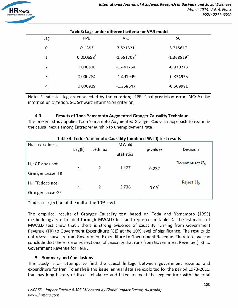
Table3: Lags under different criteria for VAR model

Notes:* indicates lag order selected by the criterion; FPE: Final prediction error, AIC: Akaike information criterion, SC: Schwarz information criterion,

4-3. Results of Toda Yamamoto Augmented Granger Causality Technique: The present study applies Toda Yamamoto Augmented Granger Causality approach to examine the causal nexus among Entrepreneurship to unemployment rate.

Table 4: Todo- Yamamoto Causality (modified Wald) test results

Null hypothesis Lag(k) k+dmax

MWald

statistics p-values Decision

H0: GE does not

Granger cause TR 1 0.232

H0: TR does not

Granger cause GE 1 0.09*

*indicate rejection of the null at the 10% level The empirical results of Granger Causality test based on Toda and Yamamoto (1995) methodology is estimated through MWALD test and reported in Table: 4. The estimates of MWALD test show that , there is strong evidence of causality running from Government Revenue (TR) to Government Expenditure (GE) at the 10% level of significance. The results do not reveal causality from Government Expenditure to Government Revenue. Therefore, we can conclude that there is a uni-directional of causality that runs from Government Revenue (TR) to Government Revenue for IRAN.

5. Summary and Conclusions This study is an attempt to find the causal linkage between government revenue and expenditure for Iran. To analysis this issue, annual data are exploited for the period 1978-2011. Iran has long history of fiscal imbalance and failed to meet the expenditure with the total

Lag FPE AIC SC

0 0.1281 3.621321 3.715617

1 0.000658* -1.651708* -1.368819*

2 0.000816 -1.441754 -0.970273

3 0.000784 -1.491999 -0.834925

4 0.000919 -1.358647 -0.509981


ISSN: 2222-6990


collected revenues. There are different theoretical viewpoints on the linkage between government spending and revenue. For example, Freidman (1978) argues that revenue causes expenditure and Barro (1979) as well as Peacock and Wiseman (1979) are of the views that government spending enhances government revenue. The determination of the causal ordering between these two macroeconomic aggregates is vital to ensure enactment of appropriate tax policies and the effectiveness of fund management. We have applied time series econometric techniques such as; unit root analysis with and without structural break , Final prediction error (FPE), Akaike information criterion (AIC) and Schwarz information criterion (SC) for determine lag length of model and Toda - Yamamoto Granger causality test. Both unit root tests ADF and Zivot-Andrews unit root test found the variables to be integrated of order one. Toda - Yamamoto Granger causality test found unidirectional causality running from government revenue to government expenditure. So, these results consistent with the revenue-spend hypothesis. Our results support the Freidman (1978) and Buchanan-Wagner hypothesis that government revenues cause expenditure. References: Akike, Hirotugu 1969 “Fitting Autoregressive Models of Prediction”, Annals of the Institute of Statistical Mathematics, Vol 2, pp. 630-39. Anderson, W., M.S. Wallace, and J.T. Warner. 1986 “Government Spending and Taxation: What Causes What?”, Southern Economic Journal, Vol. 52, pp. 630-639. Baghestani,, H., and R. McNown. 1994 “Do Revenue or Expenditures Respond to Budgetary Disequilibria?” Southern Economic Journal 60, pp. 311-322. Barro, Robert J 1974 “Are Government Bonds Not Wealth?”, Journal of Political Economy, Nov.-Dec., pp. 1095-1118. Bhat, K. Sham, V. Nirmala and B. Kamaiah. 1993 "Causality between Tax Revenue and Expenditure of Indian States", The Indian Economic Journal, Vol. 40, No. 4, pp. 109-17. Blackley, R. Paul 1986 "Causality between Revenues and Expenditures and the Size of Federal Budget", Public Finance Quarterly, Vol.14, No. 2, pp. 139-56. Buchanan, James M. and Richard W. Wegner. 1977 Democracy in Deficit, Academic Press, New York.. Cheng, Benjamin S. 1999 "Causality between Taxes and Expenditures: Evidence from Latic American Countries", Vol. 23, No. 2, pp. 184-192. Friedman, M 1972 An Economist's Protest, Thomas Horton and Company, New Jersey. Friedman, M 1978 "The Limitations of Tax Limitation", Policy Review: pp. 7-14. Furstenberg George M, von, R. Jaffery Green and Jin Ho Jeong 1986 “Tax and Spend, or Spend and Tax” The Review of Economics and Statistics, May, No. 2, pp. 179-188. Granger, C. W. J. 1969 "Investigating Causal Relationship by Econometric Models and Cross Spectural Methods, Econometrica, 37, pp. 424-438. Gujarati, D. N. 2003 Basic Econometrics, McGraw Hill Education, 4th Ed., pp. 537-538. Joulfaian, D., and R. Mookerjee 1990 “The Intertemporal Relationship Between State and Local Government Revenues and Expenditures: Evidence from OECD Countries.” Public Finance, Vol. 45, pp. 109-117. Lee, J. 1997 “Money, Income and Dynamic Lag Pattern.” Southern Economic Journal, Vol. 64, pp. 97-103.


ISSN: 2222-6990


Manage, N., and M.L. Marlow. 1986 “The Causal Relation between Federal Expenditures and Receipts.”, Southern Economic Journal, Vol. 52. pp. 617-29. Marlow, Michael L and Neela Manage 1987 "Expenditures and Receipts: Testing for Causality in State and Local Government Finances", Public Choice, Vol. 53, pp. 243-55. Owoye, O. 1995 "The Causal Relationship between Taxes and Expenditures in the G7 Countries: Co-integration and Error Correction Models", Applied Economic Letters, 2, pp. 19-22. Peacock, S.M., and J. Wiseman. 1979 “Approaches to the Analysis of Government Expenditures Growth.”, Public Finance Quarterly, Vol. 7, pp. 3-23. Ram. R. 1988 “Additional Evidence on Causality between Government Revenue and Government Expenditure”, Southern Economic Journal, 54(3), pp. 763-69. Schwarz, G. 1978 “Estimating the Dimensions of a Model” Annals of Statistics, 6, pp. 461-64.

Documents

The Relationship between Government Revenue and …hrmars.com/hrmars_papers/The_Relationship_between_Government... · The Relationship between Government Revenue ... The relationship