THE RELATIONSHIP BETWEEN NOMINAL … RELATIONSHIP BETWEEN NOMINAL INTEREST RATES AND INFLATION IN SRI LANKA Thushan Wijesinghe, University Of Cincinnati, ... (Sri Lanka Telecom)

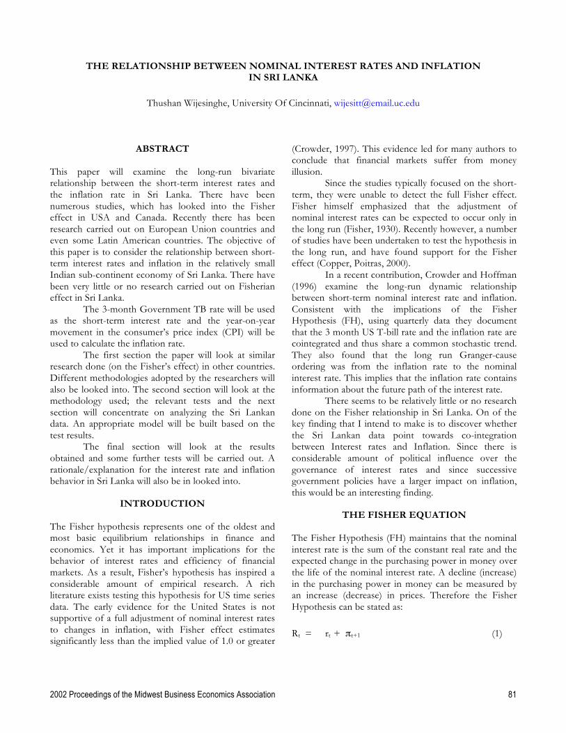
2002 Proceedings of the Midwest Business Economics Association 81

THE RELATIONSHIP BETWEEN NOMINAL INTEREST RATES AND INFLATION

IN SRI LANKA

Thushan Wijesinghe, University Of Cincinnati, [email protected]

ABSTRACT This paper will examine the long-run bivariate relationship between the short-term interest rates and the inflation rate in Sri Lanka. There have been numerous studies, which has looked into the Fisher effect in USA and Canada. Recently there has been research carried out on European Union countries and even some Latin American countries. The objective of this paper is to consider the relationship between short-term interest rates and inflation in the relatively small Indian sub-continent economy of Sri Lanka. There have been very little or no research carried out on Fisherian effect in Sri Lanka.

The 3-month Government TB rate will be used as the short-term interest rate and the year-on-year movement in the consumer’s price index (CPI) will be used to calculate the inflation rate.

The first section the paper will look at similar research done (on the Fisher’s effect) in other countries. Different methodologies adopted by the researchers will also be looked into. The second section will look at the methodology used; the relevant tests and the next section will concentrate on analyzing the Sri Lankan data. An appropriate model will be built based on the test results. The final section will look at the results obtained and some further tests will be carried out. A rationale/explanation for the interest rate and inflation behavior in Sri Lanka will also be in looked into.

INTRODUCTION

The Fisher hypothesis represents one of the oldest and most basic equilibrium relationships in finance and economics. Yet it has important implications for the behavior of interest rates and efficiency of financial markets. As a result, Fisher’s hypothesis has inspired a considerable amount of empirical research. A rich literature exists testing this hypothesis for US time series data. The early evidence for the United States is not supportive of a full adjustment of nominal interest rates to changes in inflation, with Fisher effect estimates significantly less than the implied value of 1.0 or greater

(Crowder, 1997). This evidence led for many authors to conclude that financial markets suffer from money illusion.

Since the studies typically focused on the short-term, they were unable to detect the full Fisher effect. Fisher himself emphasized that the adjustment of nominal interest rates can be expected to occur only in the long run (Fisher, 1930). Recently however, a number of studies have been undertaken to test the hypothesis in the long run, and have found support for the Fisher effect (Copper, Poitras, 2000).

In a recent contribution, Crowder and Hoffman (1996) examine the long-run dynamic relationship between short-term nominal interest rate and inflation. Consistent with the implications of the Fisher Hypothesis (FH), using quarterly data they document that the 3 month US T-bill rate and the inflation rate are cointegrated and thus share a common stochastic trend. They also found that the long run Granger-cause ordering was from the inflation rate to the nominal interest rate. This implies that the inflation rate contains information about the future path of the interest rate.

There seems to be relatively little or no research done on the Fisher relationship in Sri Lanka. On of the key finding that I intend to make is to discover whether the Sri Lankan data point towards co-integration between Interest rates and Inflation. Since there is considerable amount of political influence over the governance of interest rates and since successive government policies have a larger impact on inflation, this would be an interesting finding.

THE FISHER EQUATION The Fisher Hypothesis (FH) maintains that the nominal interest rate is the sum of the constant real rate and the expected change in the purchasing power in money over the life of the nominal interest rate. A decline (increase) in the purchasing power in money can be measured by an increase (decrease) in prices. Therefore the Fisher Hypothesis can be stated as:

Rt = rt + πt+1 (1)


Where Rt is the nominal interest rate, rt is the real interest rate, πt+1 is the expected inflation rate from period t to t+1.

If the ex-ante real rate of interest is assumed to be constant, then self-interested economic agents will require a nominal rate of interest that not only compensates for the marginal utility of the current consumption foregone (or the opportunity cost) which is measured by the real interest rate, but that compensates also for the decline in the purchasing power of money over the term of the loan. The decline in purchasing power of money is usually captured by the price inflation that is expected to occur over the life of the loan (Crowder, 1997). Therefore the Fisher equation can be restated as: Rt = rt + Et(πt+1) (2) Where, Et is the expectation operator in period t. Inflicting a rational expectation implies that equation (2) can be restated as; Rt = rt + πt+1 + εt+1 (3) where, εt+1 is the rational expectations of the forecast error. When economic agents are uncertain about their future consumption path, there will also be a risk premium term in the Fisher equation. Two studies done in 1993 (Smith) and in 1996 (Ireland) found that in the United States this risk premium is negligible.

Equation (3) demonstrates that the changes in inflation should be reflected by equal changes in the nominal interest rates when the real rate is assumed to be constant. The response of nominal interest rates to (expected) inflation has been called the “Fisher Effect”. Therefore equation (3) implies a Fisher effect of one. When nominal interest rates are subject to taxation, the tax-adjusted Fisher equation can be given by, Rt = [1 / (1 - τ)]*rt + [1 / (1 - τ)]*(πt+1) + [1 / (1 - τ)]* εt+1 (4) where, τ is the average marginal tax rate. The above equation is derived on the premise that when the nominal interest rate is taxed at the rate of τ, the after tax return is Rt*(1-τ) in equation (3), say from a lender’s perspective. Since generally τ ≥ 0, the above equation implies a Fisher effect greater than one for all tax rates greater than zero. Daly and Jung (1987) found that the personal overall average marginal tax rate in Canada was between 34.2% and 48.6%. This implied that the Fisher

effect in Canada should lie between 1.52 and 1.95 (from the calculation of [1/(1 - τ)] these values can be obtained).

LITERATURE ON THE FISHER EFFECT The literature on the Fisher effect is concentrated on two central theories. The first theory suggests that the nominal interest rate and the inflation rate are non-stationary and therefore the concept of cointegration should be used to analyze the relationship between the two variables. The alternative theory suggests that the inflation and interest rate series are not cointegrated.

Crowder (1997), states that there is little evidence on the validity of the Fisher relation in countries other than the United States. In this paper he finds support for the tax adjusted Fisher hypothesis with Canadian data. The short-term Canadian nominal interest rate and inflation rate are consistent with time series that possess a stochastic trend. He further reveals that the two series share the same stochastic trend such than they are cointegrated.

COINTEGRATION Crowder (1997) covers most academic literature in this area. He cites Rose (1988) who suggested that in the United States Rt (nominal interest rate) is non-stationary, while πt+1 (inflation rate) is stationary. Since εt+1 , the rational expectations of the forecast error in equation (3) should be stationary by definition and a linear combination of a non-stationary and a stationary variable is itself non-stationary, this result imply that in the United States, the ex post real interest rate is non-stationary. Rose (1988) further suggests that this result in incompatible with the equilibrium models of the economy which implies a stationary real rate.

If both the nominal interest rate and the inflation rate are non-stationary, then a stationary real interest rate can be simplified by the concept of Cointegration. Under cointegration, two or more variables share a long-run equilibrium such that a unique linear combination of them is stationary. In 1992, Miskin show support for the case of cointegrated nominal interest rates and inflation in the United States.

Fisher and Seater (1993) mention that the long-run neutrality tests are insufficient in the presence of cointegration. In particular, if the inflation rate and the interest rate series are non-stationary and cointegrate, then a finite vector auto regressive process in the first differences does not exist and this is typically sufficient


for rejecting the Fisherian link between inflation and short-term nominal interest rates.

Koustas & Serletis (1998) tests the long-run neutrality proposition that normal interest rates move one-to-one with inflation in the long-run, meaning that a permanent change in the rate of inflation has no long-run effect on the level of real interest rate - the Fisher relation.

We could test the null hypothesis of no cointegration (against the alternative of cointegration) using the Engle and Granger (1987) two-step procedure. This involves regressing one variable against the other to obtain the OLS regression residuals ε . A test of the null hypothesis of no cointegration (against the alternative of cointegration) is then based on testing for a unit root in the regression residuals ε using the ADF test and critical values, which correctly takes into account the number of variables in the cointegration regression.

SRI LANKAN DATA The data for the research was obtained from the Institute of Policy Studies (IPS) and the Central Bank of Sri Lanka (CBSL). The next section looks at the behavior of the two key variables over the sample range and explains such behavior in the Sri Lankan context.

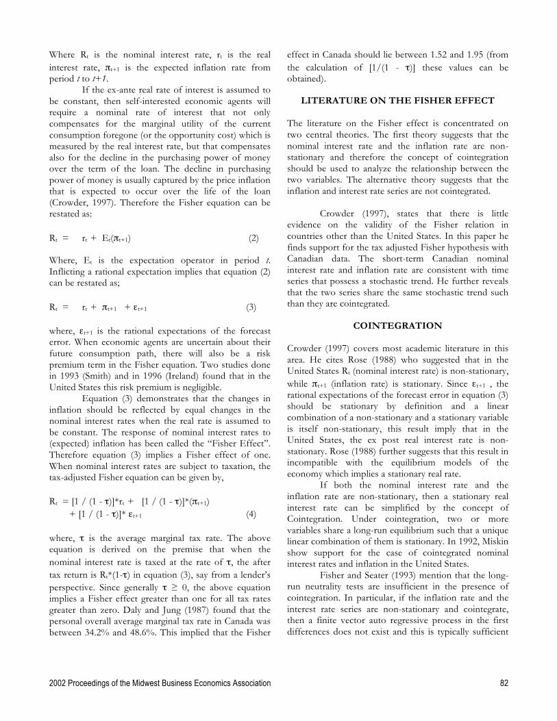
INFLATION AND 3 MONTH TB RATES Since gaining Independence from the British in 1948, Sri Lanka had an agriculture-based economy and was governed by conservatism. The policy was more of a “controlled economy” and there were few if any imports. As a result, the inflation rate was kept at a low level during the 1960’s. During the mid 1970’s with a pro-leftist party governing the country, the effects of these policies were more than felt. In 1978 a major change of government took place. The new party changed the economic policy to an “open” one in 1979 resulting in a spate of imported goods. This factor drove the inflation rate to a record high of 26.1% in 1980.

The first few years in the 80’s decade continued to have high inflation as the country accustomed itself to the “open economy”. Since then the inflation rate has been hovering around 10-12% apart from two outliers. These outliers occurred during years 1989 and 1996. During 1989 there was civil unrest in the country and in 1996 country went into a deep power crisis. The industrial production faced a very hard time.

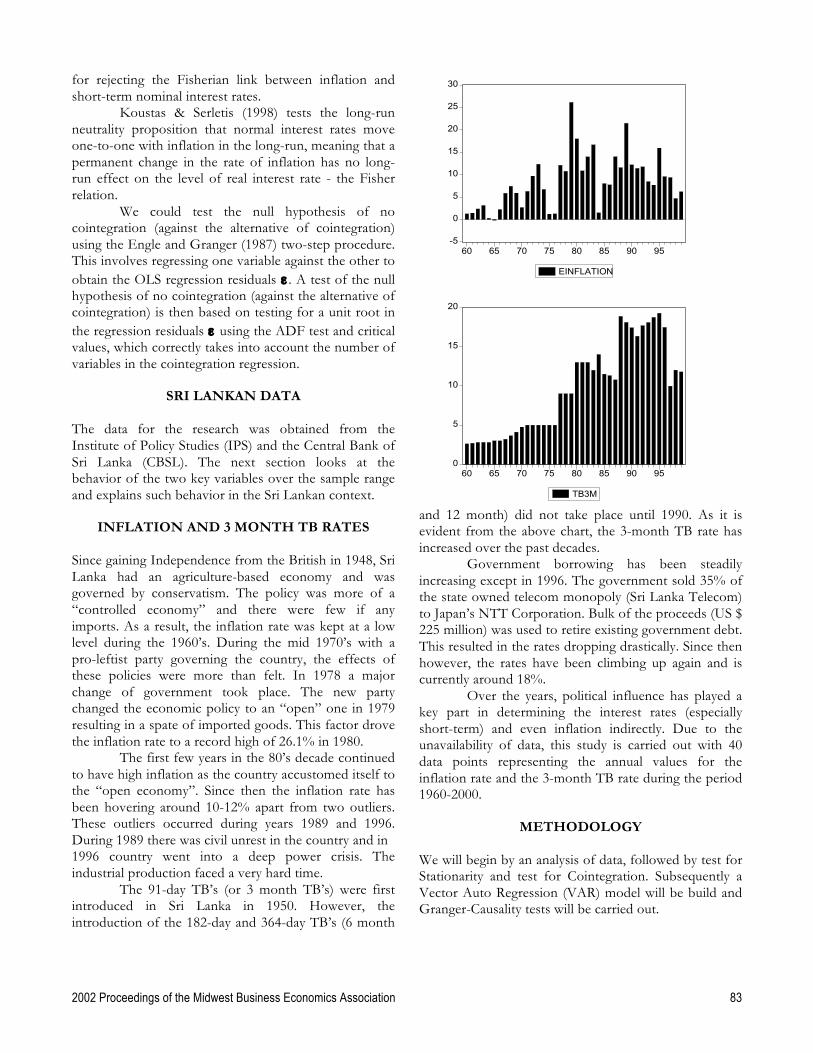
The 91-day TB’s (or 3 month TB’s) were first introduced in Sri Lanka in 1950. However, the introduction of the 182-day and 364-day TB’s (6 month

and 12 month) did not take place until 1990. As it is evident from the above chart, the 3-month TB rate has increased over the past decades.

Government borrowing has been steadily increasing except in 1996. The government sold 35% of the state owned telecom monopoly (Sri Lanka Telecom) to Japan’s NTT Corporation. Bulk of the proceeds (US $ 225 million) was used to retire existing government debt. This resulted in the rates dropping drastically. Since then however, the rates have been climbing up again and is currently around 18%.

Over the years, political influence has played a key part in determining the interest rates (especially short-term) and even inflation indirectly. Due to the unavailability of data, this study is carried out with 40 data points representing the annual values for the inflation rate and the 3-month TB rate during the period 1960-2000.

METHODOLOGY We will begin by an analysis of data, followed by test for Stationarity and test for Cointegration. Subsequently a Vector Auto Regression (VAR) model will be build and Granger-Causality tests will be carried out.

-5

0

5

10

15

20

25

30

60 65 70 75 80 85 90 95

EINFLATION

0

5

10

15

20

60 65 70 75 80 85 90 95

TB3M


USING ACTUAL INFLATION AS AN ESTIMATOR OF EXPECTED INFLATION

We make an assumption that the inflation expectation at the current period is fully realized during the next period. There is no data or indicator available on the inflation expectations during the past 40 years, which the sample range considered for this study.

TEST FOR STATIONARITY The first step of the methodology is finding the order of integrations of the data. This is generally found using a Test for Stationarity. The test for stationary is carried out using a unit root test. A unit root test can be carried out using an Augmented Dickey-Fuller (ADF) Test or Phillips-Perron (PP) test. We would carry out ADF tests for both Inflation and the 12-month TB rate to determine their order of integration.

TEST FOR UNIT ROOT – USING AUGMENTED DICKEY FULLER (ADF) TEST

The Dickey-Fuller test, can be looked into by considering an AR (1) process:

yt = µ + ρ yt-1 + εt where µ and ρ are parameters and εt is assumed to be white noise. y is a stationary series if -1<ρ<1. If ρ=1, y is a non-stationary series (a random walk with drift); if the process is started at some point, the variance of y increases steadily with time and goes to infinity. If the absolute value of ρ were greater than one, the series would be explosive. Therefore, the hypothesis of a stationary series can be evaluated by testing whether the absolute value of ρ is less than one. Both the Dickey-Fuller and the Phillips-Perron tests take the unit root as the null hypothesis: ρ=1. Since explosive series do not make much economic sense, the null hypothesis is tested against the one-sided alternative: ρ<1.

The test is carried out by estimating an equation with yt-1 subtracted from both sides of the equation: yt - yt-1 = µ + ρ yt-1 - yt-1 + εt Δ yt = µ + γ yt-1 + εt where γ = ρ -1 and the null and alternative hypotheses are:

H0 : γ = 0; and H1 : γ < 0;

To carry out the ADF test, one needs to specify the number of lags to add to the test regression (selecting zero yields the DF test; choosing numbers greater than zero generate ADF tests). Next, the inclusion of other exogenous variables in the test regression arises. We could include a constant, a constant and a linear time trend, or neither in the test regression.

The general principle to choose a specification for the regression equation is to look at the data (Hamilton 1994a). If the series seems to contain a trend (whether deterministic or stochastic), one should include both a constant and trend in the test regression. If the series does not exhibit any trend and has a nonzero mean, only a constant should be included in the regression, while if the series seems to be fluctuating around a zero mean, neither a constant nor a trend should be included in the test regression.

The tests for inflation and interest rates were conducted using both a constant and a constant & a linear trend. The results for inflation are given in Appendix 1 (a) and for 12-month TB rate in Appendix 1 (b).

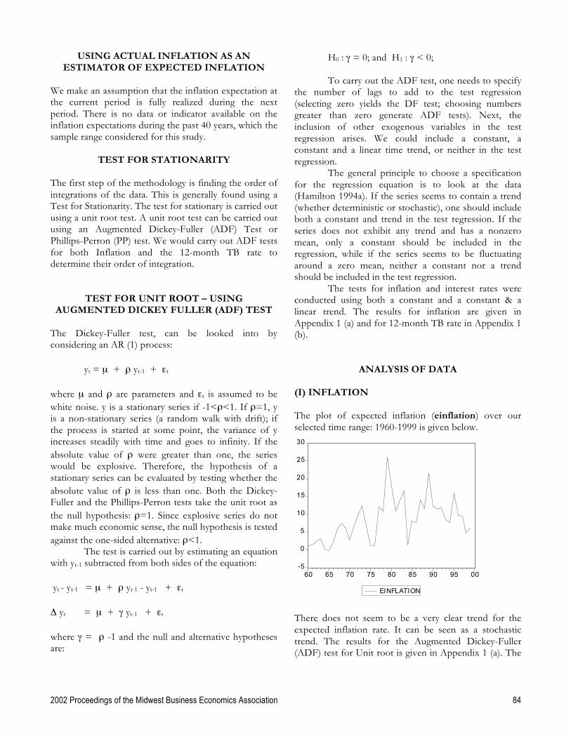
ANALYSIS OF DATA (I) INFLATION The plot of expected inflation (einflation) over our selected time range: 1960-1999 is given below.

-5

0

5

10

15

20

25

30

60 65 70 75 80 85 90 95 00

EINFLATION

There does not seem to be a very clear trend for the expected inflation rate. It can be seen as a stochastic trend. The results for the Augmented Dickey-Fuller (ADF) test for Unit root is given in Appendix 1 (a). The


test results point that einlfation is of order 1 (non-stationary) or I (1). As a result we will have to use differenced data.

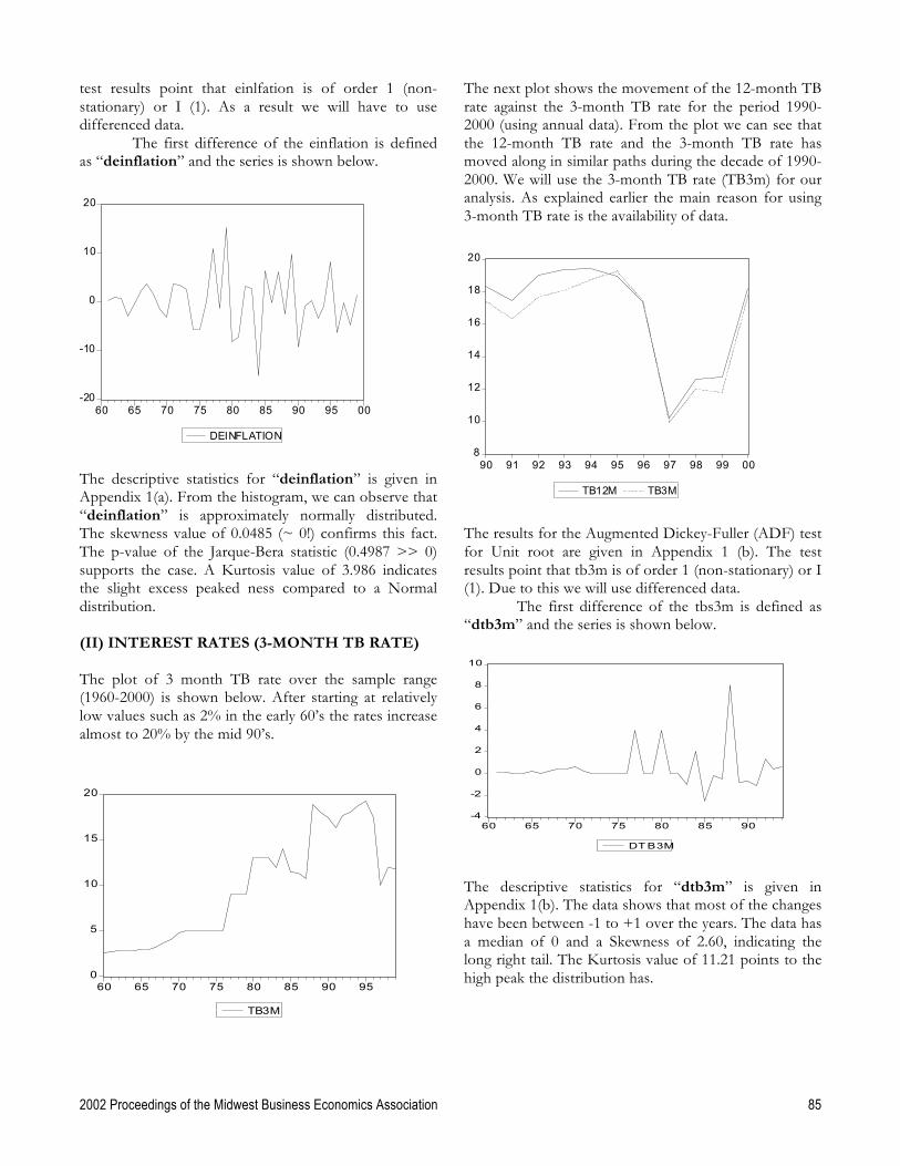
The first difference of the einflation is defined as “deinflation” and the series is shown below.

-20

-10

0

10

20

60 65 70 75 80 85 90 95 00

DEINFLATION

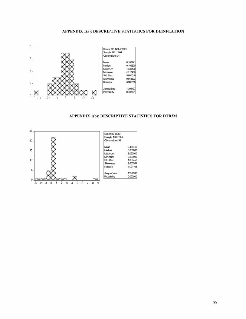
The descriptive statistics for “deinflation” is given in Appendix 1(a). From the histogram, we can observe that “deinflation” is approximately normally distributed. The skewness value of 0.0485 (~ 0!) confirms this fact. The p-value of the Jarque-Bera statistic (0.4987 >> 0) supports the case. A Kurtosis value of 3.986 indicates the slight excess peaked ness compared to a Normal distribution. (II) INTEREST RATES (3-MONTH TB RATE) The plot of 3 month TB rate over the sample range (1960-2000) is shown below. After starting at relatively low values such as 2% in the early 60’s the rates increase almost to 20% by the mid 90’s.

0

5

10

15

20

60 65 70 75 80 85 90 95

TB3M

The next plot shows the movement of the 12-month TB rate against the 3-month TB rate for the period 1990-2000 (using annual data). From the plot we can see that the 12-month TB rate and the 3-month TB rate has moved along in similar paths during the decade of 1990-2000. We will use the 3-month TB rate (TB3m) for our analysis. As explained earlier the main reason for using 3-month TB rate is the availability of data.

8

10

12

14

16

18

20

90 91 92 93 94 95 96 97 98 99 00

TB12M TB3M

The results for the Augmented Dickey-Fuller (ADF) test for Unit root are given in Appendix 1 (b). The test results point that tb3m is of order 1 (non-stationary) or I (1). Due to this we will use differenced data.

The first difference of the tbs3m is defined as “dtb3m” and the series is shown below.

-4

-2

0

2

4

6

8

10

60 65 70 75 80 85 90

DTB3M

The descriptive statistics for “dtb3m” is given in Appendix 1(b). The data shows that most of the changes have been between -1 to +1 over the years. The data has a median of 0 and a Skewness of 2.60, indicating the long right tail. The Kurtosis value of 11.21 points to the high peak the distribution has.


TEST FOR COINTEGRATION

(1) ENGLE & GRANGER TEST FOR COINTEGRATION This is the simpler of the two available tests. If two variables are found to be I (1) then we can regress them. Though the resulting regression does not make valid results, if the two variables are cointegrated, then the resulting residuals will be stationary. Therefore we can carry out a unit root test to check whether the residuals are I (0). In our model, we have found that, Rt , πt+1 ~ I (1) Therefore we can regress the two variables in the following manner. Rt = α + βπt+1 + εt (5)

where, α and β are constants and εt is the residual. The results of this regression are given in

Appendix 3 (a) and 3 (b). The test results show that the residuals are non-stationary and are of order I (1). This implies that no linear combination of the two variables is stationary and I (0).

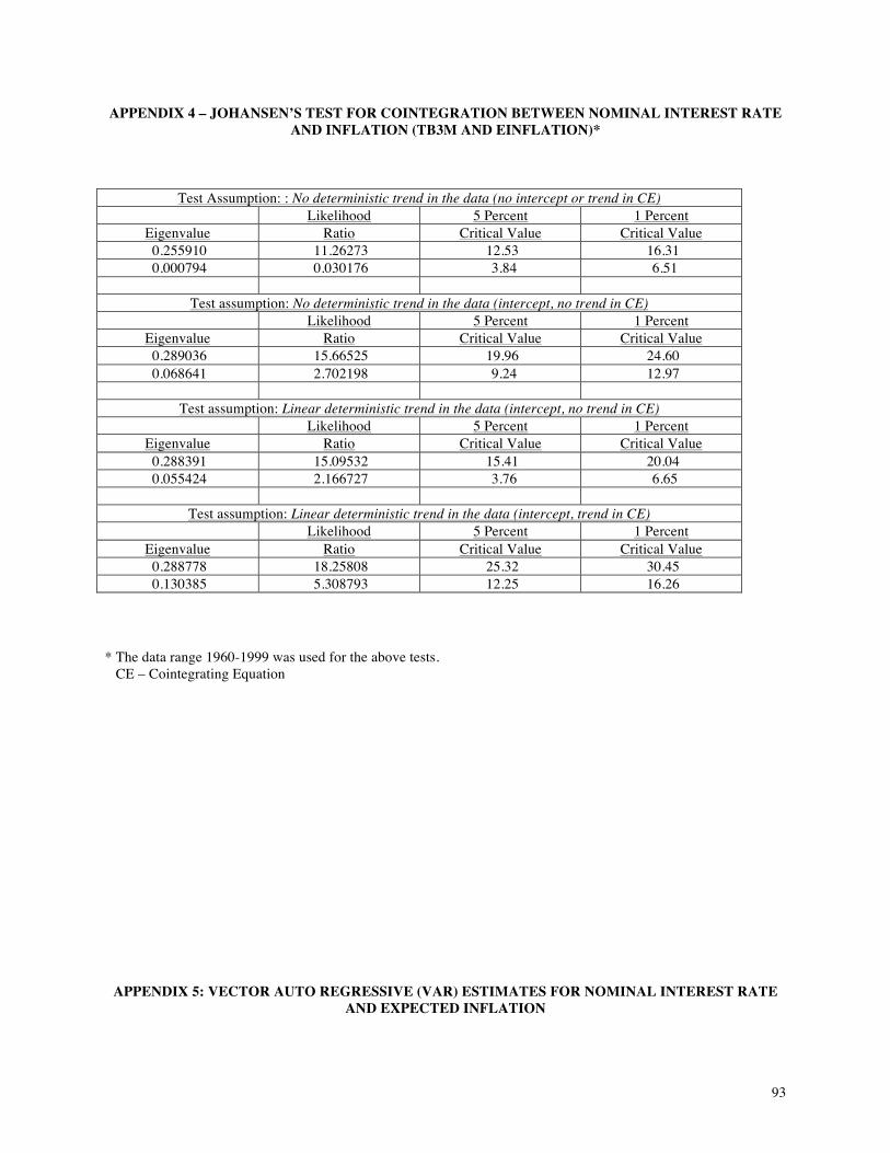
The results give us some evidence that the two variables are not cointegrated. Given the data restriction of 40 points, this would be weak evidence that the variables are not cointegrated (2) JOHANSEN’S COINTEGRATION TEST Johansen’s test of cointegration is used to determine whether a group of non-stationary series (such as the nominal interest rate and inflation) has a long-run relationship, i.e. they are cointegrated. (Johansen, Soren, 1991).

The test can be carried out assuming that there is no deterministic trend in the data (with or without an intercept) or assuming that there is a deterministic trend in the data. The results under all the categories are given in Appendix 4. It should be noted that this test again is not very powerful.

The test was carried under four assumptions (with and without deterministic trend in data and with / without intercept and trend). The results again point towards no cointegration between data. Again this would be weak evidence in the light of the data restrictions.

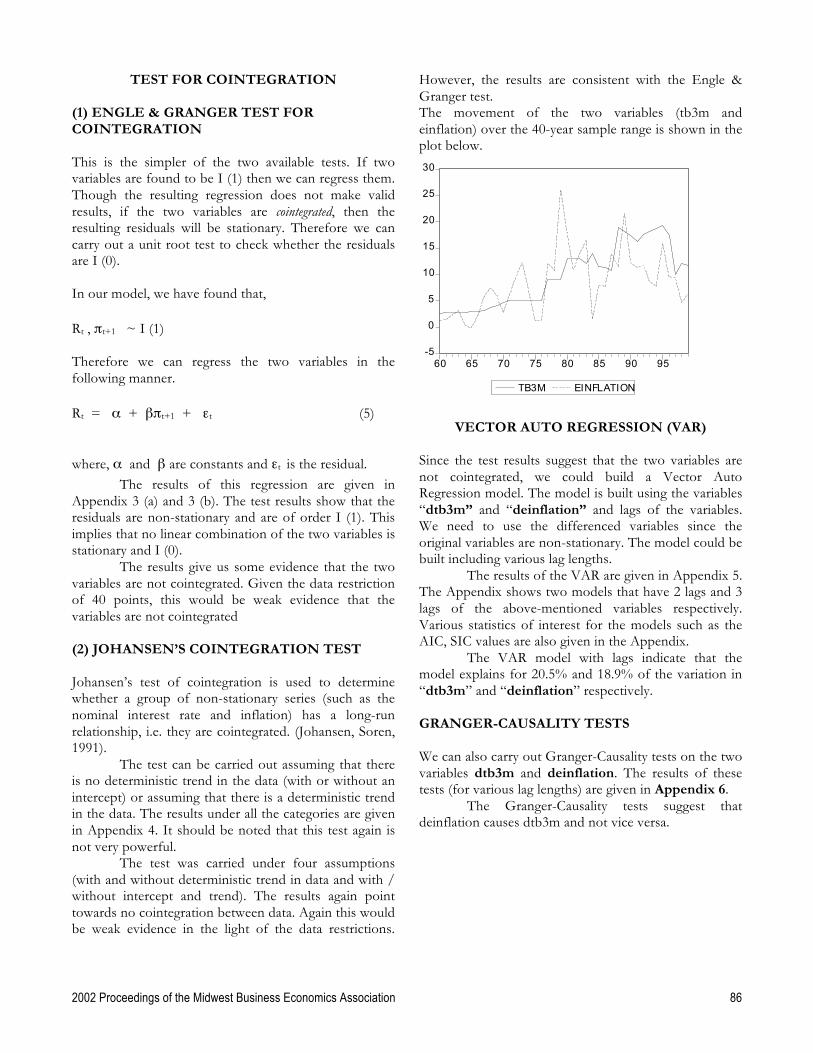
However, the results are consistent with the Engle & Granger test. The movement of the two variables (tb3m and einflation) over the 40-year sample range is shown in the plot below.

-5

0

5

10

15

20

25

30

60 65 70 75 80 85 90 95

TB3M EINFLATION

VECTOR AUTO REGRESSION (VAR)

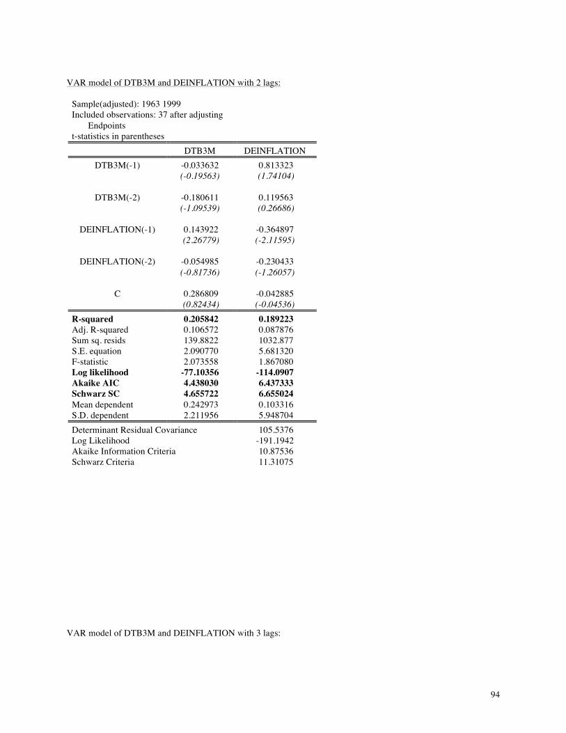
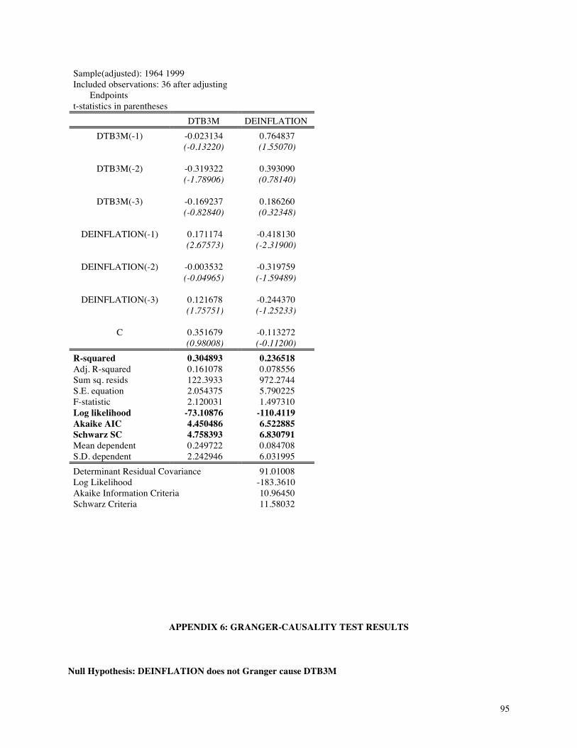
Since the test results suggest that the two variables are not cointegrated, we could build a Vector Auto Regression model. The model is built using the variables “dtb3m” and “deinflation” and lags of the variables. We need to use the differenced variables since the original variables are non-stationary. The model could be built including various lag lengths. The results of the VAR are given in Appendix 5. The Appendix shows two models that have 2 lags and 3 lags of the above-mentioned variables respectively. Various statistics of interest for the models such as the AIC, SIC values are also given in the Appendix. The VAR model with lags indicate that the model explains for 20.5% and 18.9% of the variation in “dtb3m” and “deinflation” respectively. GRANGER-CAUSALITY TESTS We can also carry out Granger-Causality tests on the two variables dtb3m and deinflation. The results of these tests (for various lag lengths) are given in Appendix 6.

The Granger-Causality tests suggest that deinflation causes dtb3m and not vice versa.


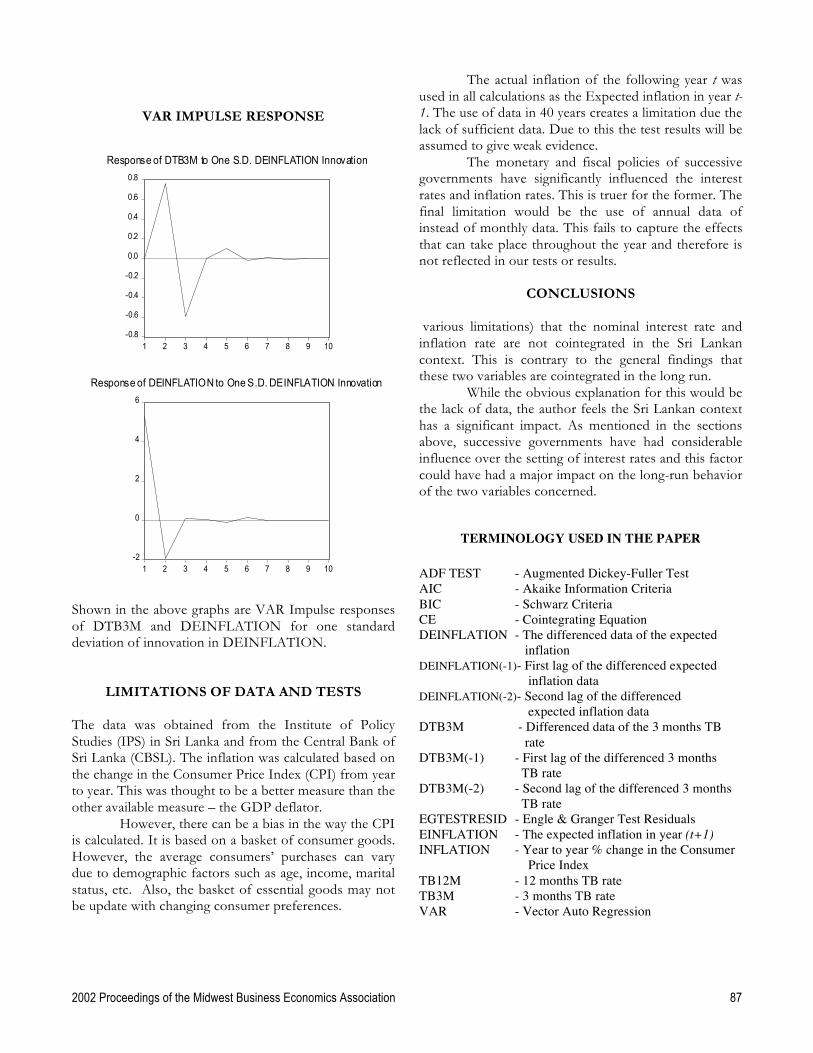
VAR IMPULSE RESPONSE

-0.8

-0.6

-0.4

-0.2

0.0

0.2

0.4

0.6

0.8

1 2 3 4 5 6 7 8 9 10

Response of DTB3M to One S.D. DEINFLATION Innovation

-2

0

2

4

6

1 2 3 4 5 6 7 8 9 10

Response of DEINFLATION to One S.D. DEINFLATION Innovation

Shown in the above graphs are VAR Impulse responses of DTB3M and DEINFLATION for one standard deviation of innovation in DEINFLATION.

LIMITATIONS OF DATA AND TESTS The data was obtained from the Institute of Policy Studies (IPS) in Sri Lanka and from the Central Bank of Sri Lanka (CBSL). The inflation was calculated based on the change in the Consumer Price Index (CPI) from year to year. This was thought to be a better measure than the other available measure – the GDP deflator.

However, there can be a bias in the way the CPI is calculated. It is based on a basket of consumer goods. However, the average consumers’ purchases can vary due to demographic factors such as age, income, marital status, etc. Also, the basket of essential goods may not be update with changing consumer preferences.

The actual inflation of the following year t was used in all calculations as the Expected inflation in year t-1. The use of data in 40 years creates a limitation due the lack of sufficient data. Due to this the test results will be assumed to give weak evidence.

The monetary and fiscal policies of successive governments have significantly influenced the interest rates and inflation rates. This is truer for the former. The final limitation would be the use of annual data of instead of monthly data. This fails to capture the effects that can take place throughout the year and therefore is not reflected in our tests or results.

CONCLUSIONS various limitations) that the nominal interest rate and inflation rate are not cointegrated in the Sri Lankan context. This is contrary to the general findings that these two variables are cointegrated in the long run.

While the obvious explanation for this would be the lack of data, the author feels the Sri Lankan context has a significant impact. As mentioned in the sections above, successive governments have had considerable influence over the setting of interest rates and this factor could have had a major impact on the long-run behavior of the two variables concerned.

TERMINOLOGY USED IN THE PAPER ADF TEST - Augmented Dickey-Fuller Test AIC - Akaike Information Criteria BIC - Schwarz Criteria CE - Cointegrating Equation DEINFLATION - The differenced data of the expected

inflation DEINFLATION(-1)- First lag of the differenced expected

inflation data DEINFLATION(-2)- Second lag of the differenced

expected inflation data DTB3M - Differenced data of the 3 months TB

rate DTB3M(-1) - First lag of the differenced 3 months

TB rate DTB3M(-2) - Second lag of the differenced 3 months

TB rate EGTESTRESID - Engle & Granger Test Residuals EINFLATION - The expected inflation in year (t+1) INFLATION - Year to year % change in the Consumer

Price Index TB12M - 12 months TB rate TB3M - 3 months TB rate VAR - Vector Auto Regression

88

APPENDIX 1(a): DESCRIPTIVE STATISTICS FOR DEINFLATION

0

2

4

6

8

-15 -10 -5 0 5 10 15

Series: DEINFLATIONSample 1961 1994Observations 34

Mean 0.188741Median 0.105300Maximum 15.36470Minimum -15.17400Std. Dev. 5.880049Skewness 0.048503Kurtosis 3.986318

Jarque-Bera 1.391497Probability 0.498701

APPENDIX 1(b): DESCRIPTIVE STATISTICS FOR DTB3M

0

5

10

15

20

25

-3 -2 -1 0 1 2 3 4 5 6 7 8 9

Series: DTB3MSample 1961 1994Observations 34

Mean 0.474412Median 0.000000Maximum 8.090000Minimum -2.500000Std. Dev. 1.800458Skewness 2.603554Kurtosis 11.21168

Jarque-Bera 133.9396Probability 0.000000

89

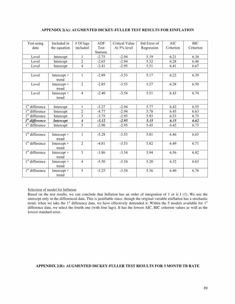
APPENDIX 2(A): AUGMENTED DICKEY-FULLER TEST RESULTS FOR EINFLATION Test using

data Included in the equation

# Of lags included

ADF Test

Statistic

Critical Value At 5% level

Std Error of Regression

AIC Criterion

BIC Criterion

Level Intercept 1 -2.75 -2.94 5.19 6.21 6.34 Level Intercept 2 -2.65 -2.94 5.32 6.28 6.46 Level Intercept 4 -2.41 -2.95 5.51 6.41 6.67

Level Intercept +

trend 1 -2.89 -3.53 5.17 6.22 6.39

Level Intercept + trend

2 -2.85 -3.53 5.27 6.28 6.50


4 -2.40 -3.54 5.51 6.43 6.74

1st difference Intercept 1 -5.27 -2.94 5.77 6.42 6.55 1st difference Intercept 2 -4.77 -2.94 5.78 6.45 6.63 1st difference Intercept 3 -3.75 -2.95 5.93 6.53 6.75 1st difference Intercept 4 -5.12 -2.95 5.35 6.35 6.62 1st difference Intercept 5 -2.90 -2.95 5.45 6.42 6.73

1st difference Intercept +

trend 1 -5.28 -3.53 5.81 6.46 6.63

1st difference Intercept + trend

2 -4.81 -3.53 5.82 6.49 6.71


3 -3.86 -3.54 5.94 6.56 6.82


4 -5.50 -3.54 5.20 6.32 6.63


5 -3.25 -3.54 5.36 6.40 6.76

Selection of model for Inflation Based on the test results, we can conclude that Inflation has an order of integration of 1 or is I (1). We use the intercept only in the differenced data. This is justifiable since, though the original variable einflation has a stochastic trend, when we take the 1st difference data, we have effectively detrended it. Within the 5 models available for 1st difference data, we select the fourth one (with four lags). It has the lowest AIC, BIC criterion values as well as the lowest standard error.

APPENDIX 2(B): AUGMENTED DICKEY-FULLER TEST RESULTS FOR 3 MONTH TB RATE

90

Test using

data Included in

equation # Of lags included

ADF Test Statistic

Critical Value At 5% level

Std Error of Regression

AIC Criterion

BIC Criterion

Level Intercept 1 -1.38 -2.94 2.17 4.46 4.59 Level Intercept 2 -1.35 -2.94 2.23 4.54 4.72 Level Intercept 4 -1.40 -2.95 2.29 4.65 4.91

Level Intercept +

trend 1 -1.79 -3.53 2.14 4.46 4.63


2 -1.80 -3.53 2.19 4.53 4.75


4 -1.64 -3.54 2.25 4.64 4.95

1st

difference Intercept 1 -4.70 -2.94 2.25 4.54 4.67

1st difference Intercept 2 -4.20 -2.94 2.27 4.58 4.76 1st difference Intercept 3 -2.39 -2.94 2.32 4.66 4.88 1st difference Intercept 4 -2.53 -2.95 2.36 4.71 4.98 1st difference Intercept 5 -1.94 -2.95 2.45 4.81 5.13

1st difference Intercept +

trend 1 -4.76 -3.53 2.26 4.57 4.75


2 -4.28 -3.53 2.28 4.61 4.83


3 -2.47 -3.54 2.32 4.66 4.94


4 -2.56 -3.54 2.36 4.74 5.05


5 -1.89 -3.54 2.44 4.83 5.19

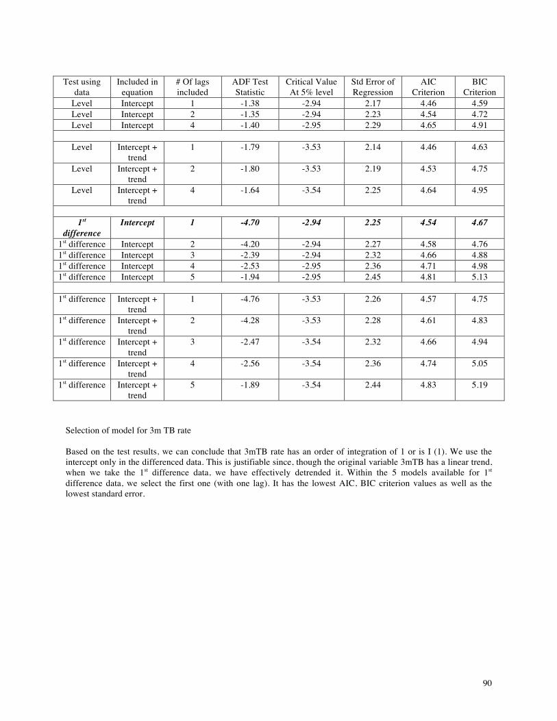
Selection of model for 3m TB rate Based on the test results, we can conclude that 3mTB rate has an order of integration of 1 or is I (1). We use the intercept only in the differenced data. This is justifiable since, though the original variable 3mTB has a linear trend, when we take the 1st difference data, we have effectively detrended it. Within the 5 models available for 1st difference data, we select the first one (with one lag). It has the lowest AIC, BIC criterion values as well as the lowest standard error.

91

APPENDIX 3(A): RESULTS OF THE REGRESSION OF RT (NOMINAL INTEREST RATE) ON πT+1 (EXPECTED INFLATION)

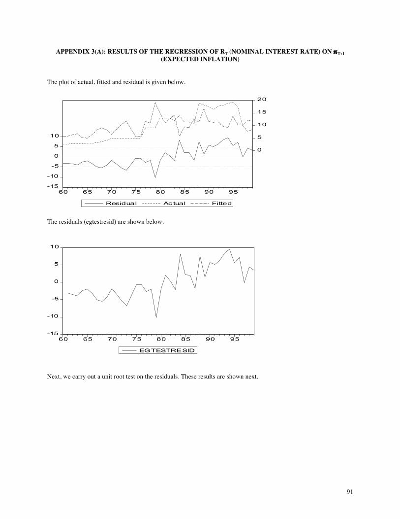
The plot of actual, fitted and residual is given below.

-15

-10

-5

0

5

10

0

5

10

15

20

60 65 70 75 80 85 90 95

Residual Ac tual Fitted

The residuals (egtestresid) are shown below.

-15

-10

-5

0

5

10

60 65 70 75 80 85 90 95

EGTESTRESID

Next, we carry out a unit root test on the residuals. These results are shown next.

92

APPENDIX 3(B): RESULTS OF THE UNIT ROOT TEST ON “EGTESTRESID” (ENGLE-GRANGER TEST RESIDUAL)

Test using data Included in the

equation # Of lags included

ADF Test Statistic

Critical Value (5% level)

Std Error Of Regression

Level Intercept 1 -1.63 -2.94 3.50 Level Intercept 2 -1.41 -2.94 3.57 Level Intercept 4 -1.01 -2.95 3.57

Level Intercept + trend 1 -3.22 -3.53 3.22 Level Intercept + trend 2 -3.02 -3.53 3.30 Level Intercept + trend 4 -2.61 -3.54 3.31

1st diff Intercept 1 -5.97 -2.94 3.63 1st diff Intercept 2 -5.97 -2.94 3.47 1st diff Intercept 4 -4.19 -2.95 3.45

1st diff Intercept + trend 1 -5.88 -3.53 3.68 1st diff Intercept + trend 2 -5.88 -3.53 3.52 1st diff Intercept + trend 4 -4.15 -3.54 3.51

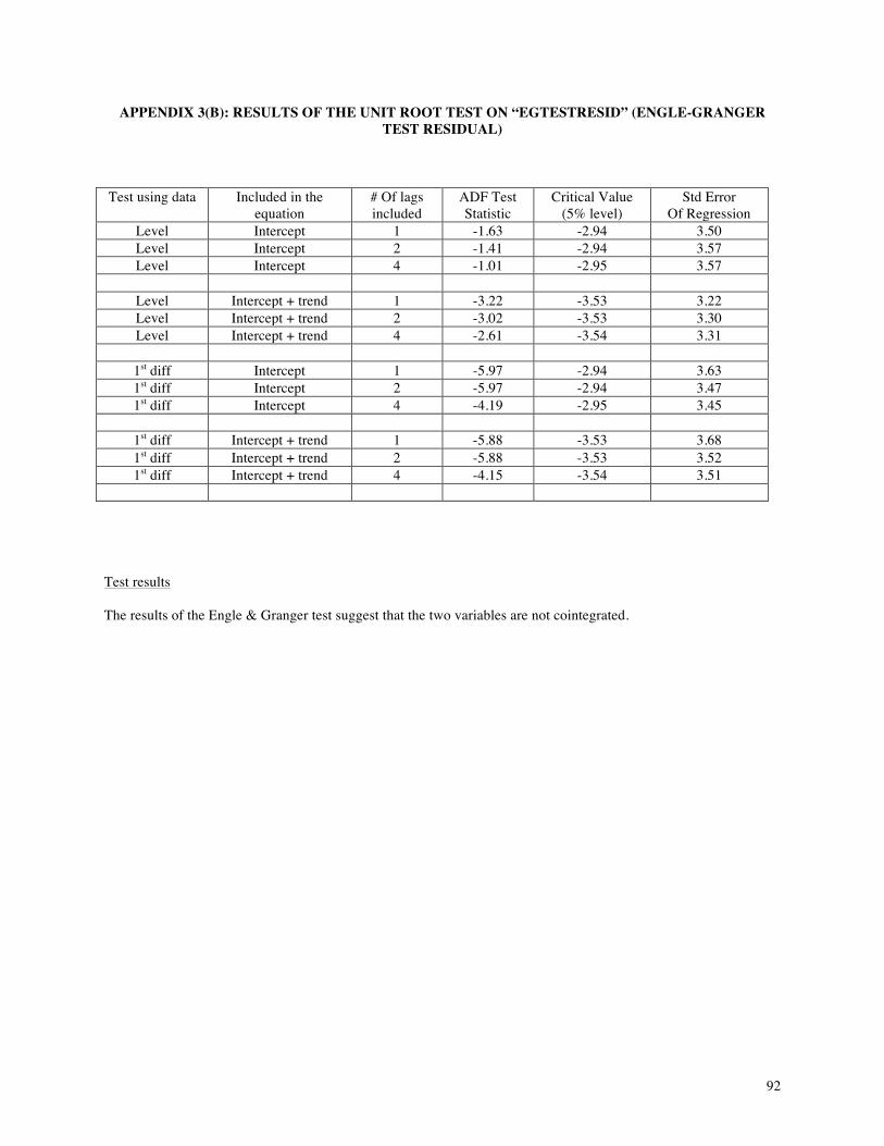
Test results The results of the Engle & Granger test suggest that the two variables are not cointegrated.

93

APPENDIX 4 – JOHANSEN’S TEST FOR COINTEGRATION BETWEEN NOMINAL INTEREST RATE AND INFLATION (TB3M AND EINFLATION)*

Test Assumption: : No deterministic trend in the data (no intercept or trend in CE) Likelihood 5 Percent 1 Percent

Eigenvalue Ratio Critical Value Critical Value 0.255910 11.26273 12.53 16.31 0.000794 0.030176 3.84 6.51

Test assumption: No deterministic trend in the data (intercept, no trend in CE)

Likelihood 5 Percent 1 Percent Eigenvalue Ratio Critical Value Critical Value 0.289036 15.66525 19.96 24.60 0.068641 2.702198 9.24 12.97

Test assumption: Linear deterministic trend in the data (intercept, no trend in CE) Likelihood 5 Percent 1 Percent

Eigenvalue Ratio Critical Value Critical Value 0.288391 15.09532 15.41 20.04 0.055424 2.166727 3.76 6.65

Test assumption: Linear deterministic trend in the data (intercept, trend in CE)

Likelihood 5 Percent 1 Percent Eigenvalue Ratio Critical Value Critical Value 0.288778 18.25808 25.32 30.45 0.130385 5.308793 12.25 16.26

* The data range 1960-1999 was used for the above tests. CE – Cointegrating Equation

APPENDIX 5: VECTOR AUTO REGRESSIVE (VAR) ESTIMATES FOR NOMINAL INTEREST RATE AND EXPECTED INFLATION

94

VAR model of DTB3M and DEINFLATION with 2 lags: Sample(adjusted): 1963 1999 Included observations: 37 after adjusting Endpoints t-statistics in parentheses

DTB3M DEINFLATION DTB3M(-1) -0.033632 0.813323

(-0.19563) (1.74104)

DTB3M(-2) -0.180611 0.119563 (-1.09539) (0.26686)

DEINFLATION(-1) 0.143922 -0.364897 (2.26779) (-2.11595)

DEINFLATION(-2) -0.054985 -0.230433 (-0.81736) (-1.26057)

C 0.286809 -0.042885 (0.82434) (-0.04536)

R-squared 0.205842 0.189223 Adj. R-squared 0.106572 0.087876 Sum sq. resids 139.8822 1032.877 S.E. equation 2.090770 5.681320 F-statistic 2.073558 1.867080 Log likelihood -77.10356 -114.0907 Akaike AIC 4.438030 6.437333 Schwarz SC 4.655722 6.655024 Mean dependent 0.242973 0.103316 S.D. dependent 2.211956 5.948704 Determinant Residual Covariance 105.5376 Log Likelihood -191.1942 Akaike Information Criteria 10.87536 Schwarz Criteria 11.31075

VAR model of DTB3M and DEINFLATION with 3 lags:

95

Sample(adjusted): 1964 1999 Included observations: 36 after adjusting Endpoints t-statistics in parentheses

DTB3M DEINFLATION DTB3M(-1) -0.023134 0.764837

(-0.13220) (1.55070)

DTB3M(-2) -0.319322 0.393090 (-1.78906) (0.78140)

DTB3M(-3) -0.169237 0.186260 (-0.82840) (0.32348)

DEINFLATION(-1) 0.171174 -0.418130 (2.67573) (-2.31900)

DEINFLATION(-2) -0.003532 -0.319759 (-0.04965) (-1.59489)

DEINFLATION(-3) 0.121678 -0.244370 (1.75751) (-1.25233)

C 0.351679 -0.113272 (0.98008) (-0.11200)

R-squared 0.304893 0.236518 Adj. R-squared 0.161078 0.078556 Sum sq. resids 122.3933 972.2744 S.E. equation 2.054375 5.790225 F-statistic 2.120031 1.497310 Log likelihood -73.10876 -110.4119 Akaike AIC 4.450486 6.522885 Schwarz SC 4.758393 6.830791 Mean dependent 0.249722 0.084708 S.D. dependent 2.242946 6.031995 Determinant Residual Covariance 91.01008 Log Likelihood -183.3610 Akaike Information Criteria 10.96450 Schwarz Criteria 11.58032

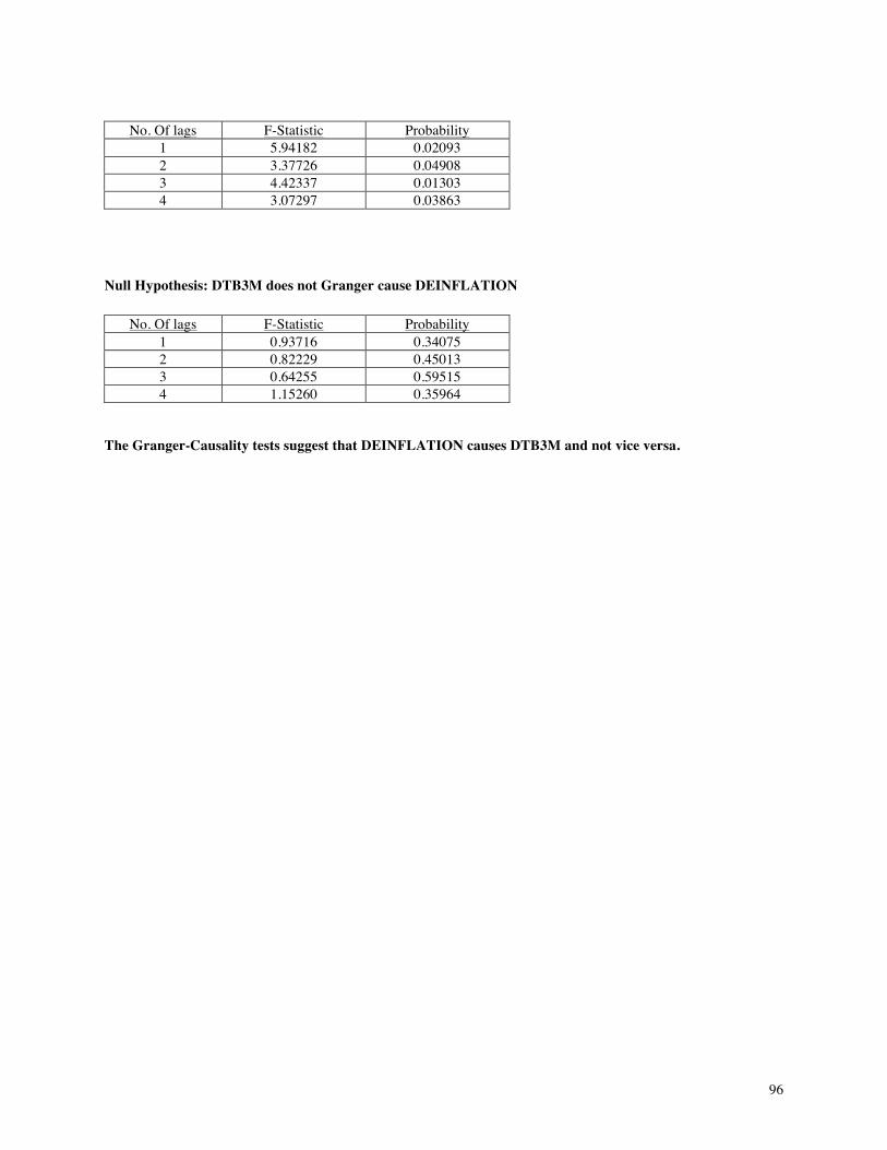
APPENDIX 6: GRANGER-CAUSALITY TEST RESULTS

Null Hypothesis: DEINFLATION does not Granger cause DTB3M

96

No. Of lags F-Statistic Probability

1 5.94182 0.02093 2 3.37726 0.04908 3 4.42337 0.01303 4 3.07297 0.03863

Null Hypothesis: DTB3M does not Granger cause DEINFLATION

No. Of lags F-Statistic Probability 1 0.93716 0.34075 2 0.82229 0.45013 3 0.64255 0.59515 4 1.15260 0.35964

The Granger-Causality tests suggest that DEINFLATION causes DTB3M and not vice versa.

97

REFERENCES Booth G.G. & Ciner C. (2000). The relationship between nominal interest rates and interest rates: international evidence. Journal of Multinational Financial Management 11 (2001) 269-280 Central Bank of Sri Lanka, Annual Report 2000 / The Statistical Abstract 1950-2000 Coppock, L. & Poitras M. (1999). Evaluating the Fisher effect in long-term cross-country averages. International review of Economics and Finance 9 (2000) 181-192 Crowder, W. J., Hoffman, D. L., (1996). The long run relationship between nominal interest rates and inflation: The Fisher equation revisited. Journal of Money Credit Bank 28, 102-118 Crowder, William (1997). The long-run Fisher relation in Canada. Canadian Journal of Economics, 30 4b (Nov 1997), 1124-1142 Dickey, D. A., Fuller, W. A., (1981). Likelihood ratio statistics for autoregressive time series with a unit root. Econometrica 49, 1057-1072 Dickey, D.A. and W.A. Fuller (1979). Distribution of the Estimators for Autoregressive Time Series with a Unit Root. Journal of the American Statistical Association 74, 427–431. Engle, R. F., Granger, C. W., (1987). Cointegration and error correction: Representation, estimation and testing. Econometrica 55, 251-276 Fisher, Irwin (1930). The theory of interest. New York Macmillan Hamilton, James D. (1994a) Time Series Analysis, Princeton University Press.

Documents

THE RELATIONSHIP BETWEEN NOMINAL … RELATIONSHIP BETWEEN NOMINAL INTEREST RATES AND INFLATION IN SRI LANKA Thushan Wijesinghe, University Of Cincinnati, ... (Sri Lanka Telecom)