Embed Size (px)
Citation preview
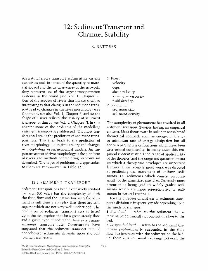
12: Sediment Transport andChannel Stability
R. BE TTESS
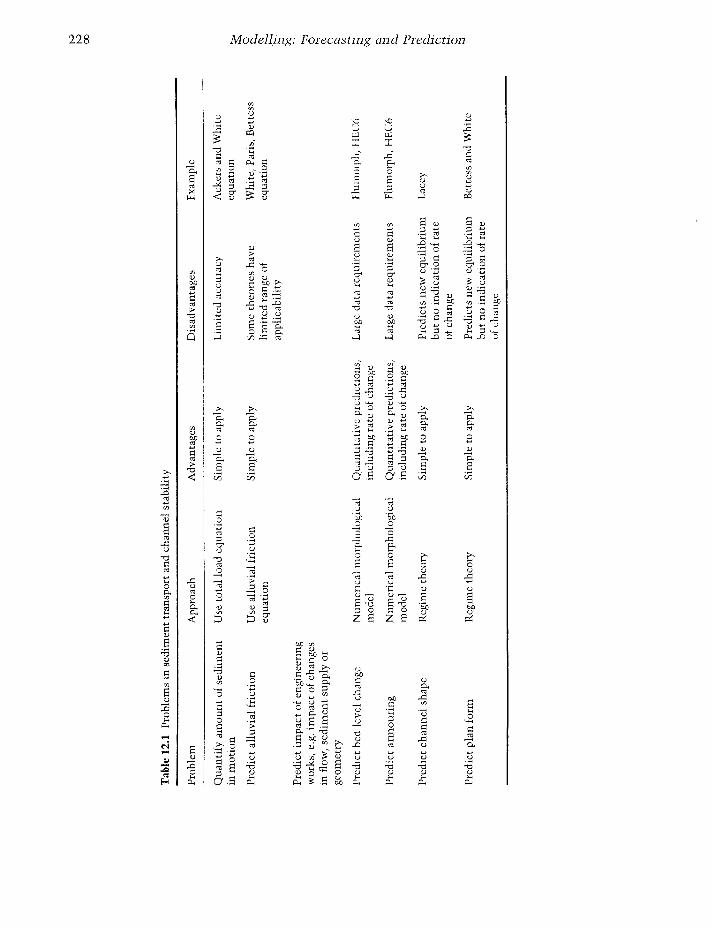
All natural nvers transport sediment in varyingquantities and, in terms of the quantity of material moved and the extensiveness of the network,they represent one of the largest transportationsystems in the world isee Vol. 1, Chapter 5).One of the aspects of rivers that makes them sointeresting is that changes in the sediment transport lead to changes in the river morphology (seeChapter 4; see also Vol. I, Chapter 6) and so theshape of a river reflects the history of sedimenttransport within it (see Vol. I, Chapter 7). In thischapter some of the problems of the modellingsediment transport are addressed. The most fundamental one is the prediction of sediment transport rate. This then leads to the prediction ofriver morphology, i.e. regime theory and changesin morpholoh7 using numerical models. An important aspect of river morphology is the planformof rivers, and methods of predicting planform aredescribed. The types of problems and approachesto them are summarized in Table 12.1.
12.1 SEDIMENT TRANSPORT
Sediment transport has been extensively studiedfor over 100 years but the complexity of boththe fluid flow and the interaction with the sediment is sufficiently complex that there are stillaspects which arc not very well understood. Theprediction of sediment transport rate is basedupon the assumption that for a given steady flowand a given type of sediment there is a uniquesediment transport rate. Observations havesuggested that the sediment transport rate ofnoncohesive sediments depends upon the following parameters:
1 Flow:velOCitydepthshear veIocitykinematic viscosityfluid density.
2 Sediment:sediment sizesediment density.
The complexity of phenomena has resulted in allsediment transport theories having an empiricalcontent. Most theories are based upon some broadtheoretical approach such as energy, efficiencyor minimum rate of energy dissipation but allcontain parameters or functions which have beendetermined empirically. In many cases this empirical content restricts the range of applicabilityof the theories, and the range and quantity of dataon which a theory was developed are importantfeatures. Until recently most work was directedat predicting the movement of uniform sediments, i.e. sediments which consist predominantly of the same sized particles. Currently moreattention is being paid to widely graded sediments which are more representative of sediments in natural channels.
For the purposes of analysis of sediment transport a division is frequently made depending uponthe mode of transport.1 Bed lood - refers to the sediment that ismoving predominantly in contact or close to thebed.2 Suspended load --- refers to the sediment thatmoves predominantly suspended in the fluidflow but interacts with the sediment on the bed;i.e. there is a continual exchange between the
227The Rivers Handboolz: Hydrological and Ecological PrinciplesEdited by Peter Calow and Geoffrey E. Petts© 1994 Blackwell Science Ltd. ISBN: 978-0-632-02985-3
Tab
le12
.1P
rob
lem
sin
sed
imen
ttr
ansp
ort
and
chan
nel
stab
ilit
y
tv tv 00
Pro
ble
m
Qu
anti
fyam
ou
nt
ofse
dim
ent
inm
oti
on
Pre
dic
tal
luv
ial
fric
tion
Pre
dic
tim
pac
tof
engi
neer
ing
wo
rks,
e.g.
imp
act
ofch
ange
sin
flow
,se
dim
ent
supp
lyo
rg
eom
etry
Pre
dic
tb
edle
vel
chan
ge
Pre
dic
tar
mo
uri
ng
Pre
dic
tch
ann
elsh
ape
Pre
dic
tp
lan
form
App
roac
h
Use
tota
llo
adeq
uat
ion
Use
allu
vial
fric
tio
neq
uat
ion
Nu
mcr
ical
mo
rph
olo
gic
alm
odel
Nu
mer
ical
mo
rph
olo
gic
alm
od
el
Reg
ime
theo
ry
Reg
ime
theo
ry
Adv
anta
ges
Sim
ple
toap
ply
Sim
ple
toap
ply
QU
dnti
tati
vepr
edic
tion
s,in
clu
din
gra
teo
fch
ange
Qu
anti
tati
ve
pred
icti
ons,
incl
ud
ing
rate
ofch
ange
Sim
ple
toap
ply
Sim
ple
toap
ply
Dis
adv
anta
ges
Lim
iteu
accu
racy
Som
eth
eori
esh
ave
lim
ited
ran
ge
ofap
pli
cab
ilit
y
Lar
ged<
ll<1
rcqu
Hcl
llcn
ls
Lar
ged
ata
req
uir
emen
ts
Pre
dic
tsn
eweq
uil
ibri
um
bu
tn
oin
dic
atio
nof
rate
ofch
ang
e
Pre
dict
sn
eweq
uil
ibri
um
bu
tn
oin
dic
atio
nof
rate
u[c
hau
ge
Exa
mpl
e
Ack
ers
anu
Whi
teeq
uati
on
Whi
te,
Par
is,
Bet
tess
equ
atio
n
rluI
llor
ph,
llE
C(;
Flu
mor
ph,
HE
C6
Lac
ey
Bet
tess
and
Wh
ite
~ a ~ ~ -5- ~ 6J ...., ~ \l l:::i
Vl ...... 5- O
q l::l b ~ ~ ...., (\:J Q ......
\) ...... g'
Sediment Transport and Channel Stability
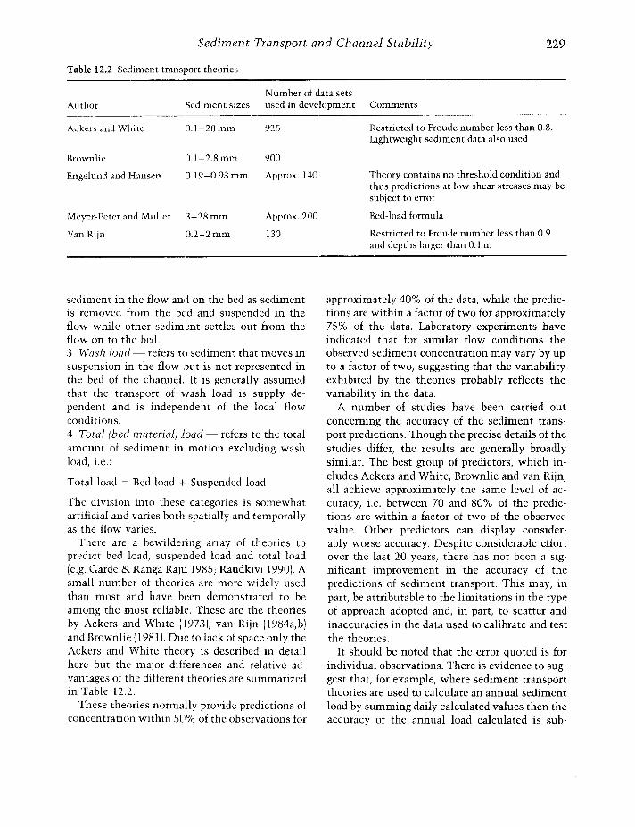
Table 12.2 Sediment transport theories
229
Author
Ackers and White
Number of data setsSediment sizes used in development Comments
0.1- 28 mm 92.5 Restricted to Froude number less than 0.8.Lightweight sediment data also used
Brownlie 0.1~2.8mrn 900
Engelund and Hansen 0.19-0.93mm Approx.140
Meyer-Peter and Muller 3-28 mm Approx. 200
Van Rijn 0.2-2mm 130
sediment in the flow and on the bed as sedimentis removed from the bed and suspended in theflow while other sediment settles out from theflow on to the bed.3 Wash load - refers to sediment that moves insuspension in the flow but is not represented inthe bed of the channel. It is generally assumedthat the transport of wash load is supply dependent and is independent of the local flowconditions.4 Total (bed material) load - refers to the totalamount of sediment in motion excluding washload, i.e.:
Total load = Bed load + Suspended load
The division into these categories is somewhatartificial and varies both spatially and temporallyas the flow varies.
There are a bewildering array of theories topredict bed load/ suspended load and total load(e.g. Garde & Ranga Raju 1985; Raudkivi 1990). Asmall number of theories are more widely usedthan most and have been demonstrated to beamong the most reliable. These are the theoriesby Ackers and White (1973', van Rijn (l984a}b)and Brownlie (1981). Due to lack of space only theAekers and White theory is described in detailhere but the major differences and relative advantages of the different theories are summarizedin Table 12.2.
These theories normally provide predictions ofconcentration within 50% of the observations for
Theory contains no threshold condition andthus predictions at low shear stresses may besubject to error
Bed-load formula
Restricted to Froude number less than 0.9and depths larger than 0.1 m
approximately 40% of the data/ while the predictions are within a factor of two for approximately75 1}"0 of the data. Laboratory experiments haveindicated that for similar flow conditions theobserved sediment concentration may vary by upto a factor of two, suggesting that the variabilityexhibited by the theories probably reflects thevariability in the data.
A number of studies have been carried outconcerning the accuracy of the sediment transport predictions. Though the precise details of thestudies differ, the results are generally broadlysimilar. The best group of predictors) which includes Ackers and White/ Brownlie and van Rijn/all achieve approximately the same level of accuracy, i.e. between 70 and 80% of the predictions are within a factor of two of the observedvalue. Other predictors can display considerably worse accuracy. Despite considerable effortover the last 20 years/ there has not been a significant improvement in the accuracy of thepredictions of sediment transport. This may} inpart/ be attributable to the limitations in the typeof approach adopted and/ in part, to scatter andinaccuracies in the data used to calibrate and testthe theories.
It should be noted that the error quoted is forindividual observations. There is evidence to suggest that} for example/ where sediment transporttheories are used to calculate an annual sedimentload by summing daily calculated values then theaccuracy of the annual load calculated is sub-
230 Modelling: Forecasting and Prediction
that the total transport of bed material may becalculated directly.
The hypothesis was that n could be evaluated byanalysing flume data for a range of sediment sizesand should lie between 0 and 1, showing a continuous variation through coarse material and
where V* is the shear velocity, V is the velocity offlow, D is the sediment diameter, d is the depthof flow, g is the acceleration due to gravity and sis the sediment specific gravity. n and a are parameters, the latter usually assigned the value 10.For coarse sediments (11 = 0) the expression reduces to the form:
Sediment mobility
The original development of the theory is summarized in Ackers and White (1973:'. In essence, acoarse sediment is considered to be transportedmainly as a bed process. If bed features exist, it isassumed that the effective shear stress bears asimilar relationship to mean stream velocity aswith a plane, grain-textured surface at rest.
A fine sediment is considered to be transportedwithin the body of the flow, where it is suspendedby the stream turbulence. As the intensity of tur~
bulence is dependent on the total energy degradation, rather than on a net grain resistance, forfine-grained material the total bed shear stress iseffective in causing sediment transport.
Sediment mobility is described by the ratio ofthe effective shear force on a unit area of the bedto the immersed weight of a layer of grains. Thismobility number is denoted by Fgrl and definedby:
(3)
(2\
(11
and for fine sediments (n = 1):
Fgr = V!gD(s -- 1)]
F- V _1__gr - ,/[gD(s ~ 1l] (ad')
V3210g lO D
11'1 [ V ]l-llF" ~ \/lgDls -- III \/3210g
1O(~t
Ackers and White sediment transport theory
In many methods (Task Committee 1971; Cole etal 1973; Raudkivi 1990), shear stress is llsed asthe main parameter defining the stream's transporting power. However, the total shear on adeformed bed, rippled or duned, is, in part, composed of the along-stream components of thenormal pressures on the irregular bed profile.These normal pressures may contribute indirectlyto sediment motion through suspension, yetmany methods separate the bed shear into a nontransporting form loss and the shear on the grains.As the rate of transport is very sensitive to transporting power, inaccuracy in this shear separationprocedure may give large errors of prediction. Inengineering practice, this factor is important because few natural streams have a plane bed.
Other methods utilize stream power or averagevelocity against which the transport rate is correlated. Whatever the basis! care must be exercisedwhen applying any method because it is notalways clear whether the equation relates to thetotal load of bed material or to some ill-definedfraction of it, for example, the contact load. Itwas because of deficiencies of many previousmethods that Ackers and White developed a newframework for the analysis of sediment transportdata, which could be used predictively.
The Ackers and White method avoided refinements that complicated the application withoutadding much to accuracy. The advantages of dimensional analysis were incorporated, but physical arguments were used in deriving the form ofthe functions. The variables used were directlyrelated to those the engineer can readily visualizeand measure, and the uncertainty of slope separation procedures was avoided. The various coef~
ficients were expressed as algebraic functions so
stantially better than for the individual values.This probably arises as the errors between thepredicted and observed are normally distributedand by summing a large number of normal variates the standard deviation is reduced substantially. This also explains the success of numericalmorphological models in making long-term morphological predictions.
Sediment Transport and Channel Stability 231
transitional sizes to fine non-cohesive sand orsilt.
where Ggr is the sediment transport rate (dimensionless), and X is the sediment concentration byweight.
Dimensionless grain diameter
A dimensionless expression for grain diameterean be derived by eliminating shear stress fromthe two Shields parameters (Shields 1936': orderived from the drag coefficient and Reynoldsnumber of a settling particlc, by eliminating thescttling velocitYi or dimensionally, withimmersed weight of an individual grain, fluiddensity and viscosity as the variables. The dimensionless grain diameter, D gn is therefore generallyapplicable to coarse, transitional and finesediments and is the cube root of the ratioof the immersed weight to the viscous forces. Thefollowing expression characterizmg sedimentdiameter remains constant in anyone set ofexperiments:
Sediment transport
The expressions for sediment transport werebased on the stream power concept" in the case ofcoarse sediments using the product of net grainshear and stream velocity as the power per unitarea of bed) and for fine sediments using the totalstream power.. The useful work done in sedimenttransport in the two cases takes account of thedifferent modes of transport assumed, and in relation to the stream power gives an expression forthe efficiency of the transport process. Efficiencywas expected to be dependent on the mobilitynumber, Fgr. Clearly there would be a value of Fgrat which sediment motion first began to takeplace. As Fgr rises above this limiting value, itwas expected that the efficiency would increase.
In order to separate the primary variables, theefficiency (which is dimensionless) was combinedwith the mobility number, Fgr} to yield a generaltransport parameter:
General transport function
The relationship for Glif was assumed to be of theform:
(9'
(7)
(6)
(8)
(11)
(12)
(13)
(14'
For coarse sediments) D gr > 60:
n = 0.00
A = 0.17
m = 1.50
C = 0.025
For transitIOnal sizes, 1 < D gr < 60:
n = 1.00 - 0.56 log10 Dgr
A = 0.23 0 14VDgr
+ .
m = 9.66 + 1.34D gr
logw C = 2.86 log 10 Dgr - (lOglO Dgr)2 - 3.53 110)
6.83 1.67 for 1 ~ Dgr ~ 60In = - + (15)
Dgr 1.78 for Dgr ~ 60
and loge = 2.791ogDgr - 0.98(logDgrf - 3.46for 1 ~ D gr ::::; 60
and C = 0.025 for Dgr ~ 60 (l6)
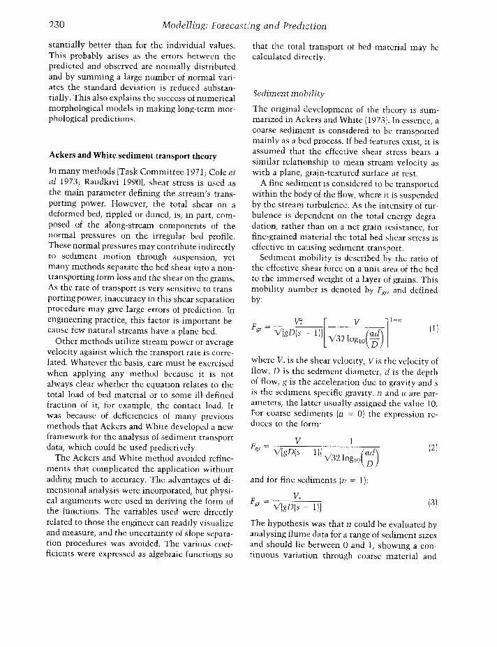
A value for a of 10 was determined. This iscomparable with the value of 12.3 which appearsin the rough~turbulentflow equation. The transport function is plotted in Fig. 12.1.
A recent study has been carried out to up-dJ.tethe values of the parameters in the light of thelarger amount of data that is now available. Thisstudy recommended:
where A, C and In are parameters. A is the valueof Fr,r at which sediment movement first beginsto take place.
Numerical optimization was used to determinebest fit values for the four parameters C, A, m andn. The resulting relationships were:
(4)
(51G = X.d[V*-jnJgr sD V_
where v is the kinematic viscosity.
_ [g(S - 11]1/3D gr - D ", v~
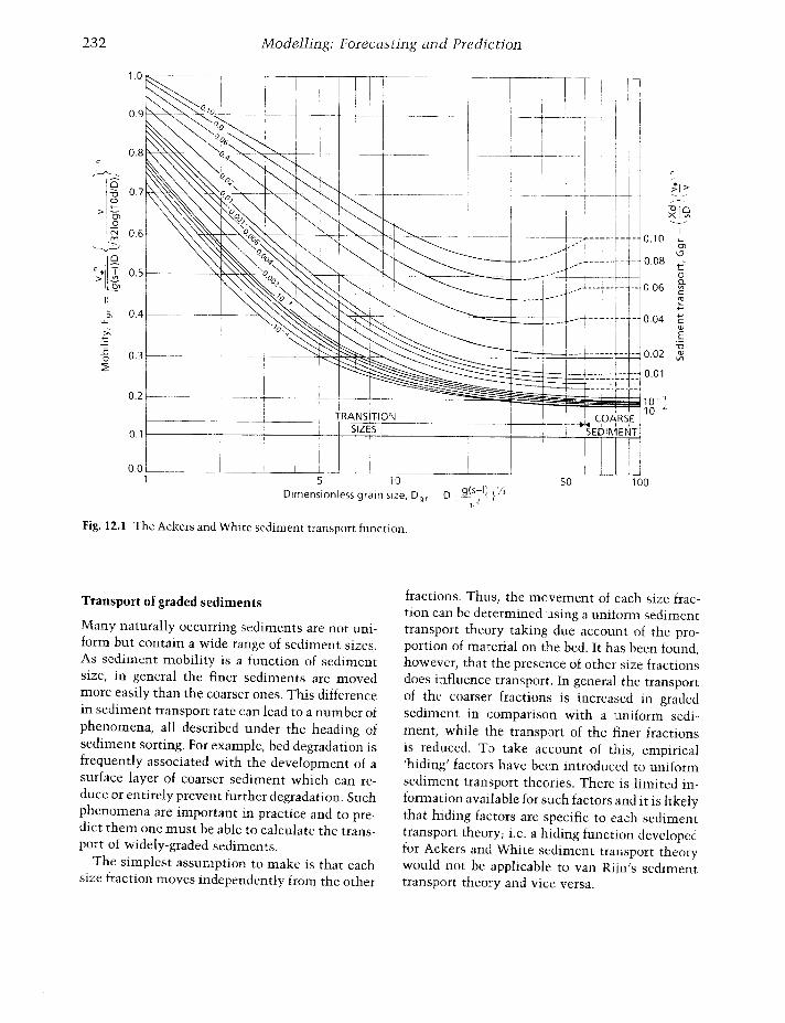
232 Modelling: Forecasting and Prediction
~i>
"010Xi V'l'--/
10050
0,4
I /0" ,
0.3 -'-~--~'T~·t-~""d"~~·-"""'"
02~+~ j-l- +-. r~., t-Tr=":=~~~~~~~~~~~~~~:gOl;
[= ... .". i.... I ",:... TR.ANSI...lIO•. N- II ····----+----tn---+-fT····..... SIZES0.1 " '+-I------+----+---+--+---,-'~____r_____T_;
I
I I
I : iO.O.J _ ' I I . ,L.t _~~~_.__-'---_. __~__-' .. _--'----'---'-----'-~
5 !O
Dimensionless grain Size, Dgr
Fig. 12.1 The Ackers and White sediment transport function.
Transport of graded sediments
Many naturally occurring sediments are not uniform but contain a wide range of sediment sizcs.As sediment mobility is a function of sedimentsizc, in general the finer sediments are movedmore easily than the coarser ones. This differencein sediment transport rate can lead to a number ofphenomena, all described under the heading ofsediment sorting. For example, bed degradation isfrequently associated with the development of asurface layer of coarser sediment which can reduce or entirely prevent further degradation. Suchphenomena arc important in practice and to predict them one must be able to calculate the transport of widely-graded sediments.
The simplest assumption to make is that eachsize fraction moves independently from the other
fractions. Thus, the movement of each size fraction can be determined 'Using a uniform sedimenttransport theory taking due account of the proportion of material on the bed. It has been found,however, that the presence of other size fractionsdoes influence transport. In general the transportof the coarser fractions is increased in gradedsediment in comparison with a uniform sediment, while the transport of the finer fractionsis reduced. To take account of this, empirical'hiding' factors have been introduced to uniformsediment transport theories. There is limited information available for such factors and it is likelythat hiding factors arc specific to each sedimenttransport theory; i.e. a hiding function developcC:for Ackers and White sediment transport theorywould not be applicable to van Rijn's sedimenttransport theory and vice versa.
Sediment Transport and Channel Stability 233
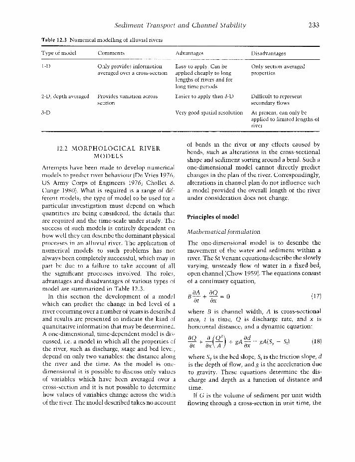
Table 12.3 Numerical modelling of alluvial rivers
Type of model Comments Advantages Disadvantages
Only section-averagedproperties
Difficult to represen t
secondary flows
Very good spatial resolution At present, can only beapplied to limited lengths ofriver
Easy to apply. Can beapplied cheaply to longlengths of rivers and forlong time penods
Easier to apply than 3-D
Only provides informationaveraged over a cross-section
Provides variation acrossse~tion
1-D
2-D, depth averaged
3-D
Principles of model
where B is channel width, A is cross-sectionalarea, t is time/ Q is discharge rate, and x 15
horizontal distance; and a dynamic equation:
where Sv is the bcd slopc, Sf is the friction slope, dis the d~pth of flow} and g is the acceleration ducto gravity. Thcse equations determine the discharge and depth as a function of distance andtime.
If G is the volume of sediment per unit widthflowing through a cross-section in unit time, the
Mathematical forrrmlation
The one-dimensional model is to describe themovement of the water and sediment within ariver. The 5t Venant equations describe the slowlyvarying
lunsteady How of water in a fixed-bed}
open channel (Chow 19591. The equations consistof a continuity equation,
(18)
(I7l
aQ a(Q2) ad- + - - + gA -;- = gAlS - Sf)at ax A ax· Y
aA aQB-- + - = 0
at ax
of bends in the river or any effects caused bybends, such as alterations in the cross-sectionalshape and sediment sorting around a bend. Such aone-dimensional model cannot directly predictchanges in the plan of the river. Correspondingly,alterations in channel plan do not influence sucha model provided the overall length of the riverunder consideration docs not change.
Attempts have been made to develop numericalmodels to predict river behaviour (De Vries 1976,US Army Corps of Engineers 1976; Chollet &Cunge 1980). What is required is a range of dif·ferent models; the type of model to be used for aparticular investigation must depend on whichquantities arc being considered, the details thatare required and the time-scale under study. Thesuccess of such models is entirely dependent onhow well they can describe the dominant physicalprocesses in an alluvial river. The application ofnumerical models to such problems has notalways been completely successful, which may inpart be due to a failure to take account of allthe significant processes involved. The roles,advantages and disadvantages of various types ofmodel are summarized in Table 12.3.
In this section the development of a modelwhich can predict the change in bed level of ariver occurring over a number of years is describedand results are presented to indicate the kind ofquantitative information that may be determined.A one-dimcnsionat time-dependent model is discussed, i.e. a model in which all the properties ofthe river, such as discharge, stage and bed level,depend on only two variables: the distance alongthe river and the time. As the model is onedimensional it is possible to discuss only valuesof variables which have been averaged over across-section and it is not possible to determinehow values of variables change across the widthof the river. The model described takes no account
12.2 .rv10RPHOLOGICAL RIVERMODELS
234 Modelling: Forecasting and Prediction
continuity equation for sediment movement maybe written as:
Sediment transport
Equation 19 implies that the only effect of anyerror in predicting the transport rate is to alter the
As discussed above there are many sedimenttransport theories of this form. Owing to thecomplexity of the processes the theories attemptto model, the predictions of the different theoriesin any particular case may vary considerably(White et al 1973).
Sediment sorting
So far only the total volume of sediment that ismoving has been considered and no attention hasbeen given to how much of each sediment size isbeing transported. For given hydraulic conditionsdifferent sediment sizes arc transported at different rates and this may lead to a restructuringof the sediment size distribution and hence tochanges in the sediment sizes used in the sediment transport calculations. Consider, for example, the movement of sediment immediatelydownstream of a newly constructed dam andassume that there is no sediment inflow, i.e. allthe sediment is trapped in the reservoir. Downstream of the dam the fine sediment will betransported more easily than the coarse sedimentand so over a period of time one would expectthe proportion of fine sediment to decrease, theproportion of coarse sediment to increase correspondingly, and the total transport rate to fall.Thus the sediment size distribution will changeand the appropriate representative sediment sizeswill alter. As the proportion of coarse sedimentwill increasc, the representative sediment size
Frictional characteristics
Concomitant with sediment transport are bedfeatures such as ripples and dunes. These featurescan change their size and form as the sedimenttransport rate varies. As such features can have asignificant effect on the frictional characteristicsof a channel, it follows that in an alluvial channel subject to considerable changes in sedimenttransport rate the roughness of the channel cannot be assumed to be fixed. To take account ofthese alterations a roughness relationship developed by White et a1 (1980) can be included. Thisis described in more detail later.
rate at which the bed of tlle river rises or falls;thus a 10% overestimate of the transport rateleads to a 10% increase in the rate of degradationof aggregation of the bed. The final equilibriumstate does not primarily depend on the transportrate although errors in the latter will affect theprediction of the time taken for this equilibriumto be achieved.
(20)
(19)
Boundary conditions
In general the time-scale associated with changesin the fluid flow is considerably shorter than thatfor variations in the bed level. It follows that, ifone is interested only in morphological changes,the fluid flow can be regarded as steady (De Vries19761. Over a short period any change in bed levelhas little effect on the fluid flow. Thus, it may beassumed that over the period of a time-step thefluid flow may be calculated independently ofthe sediment transport. Hence one may calculatethe fluid flows for a geometrically identical,fixed-bed channel and determine the velocity anddepth. These values may then be used to calculate the sediment transport, which, together withequation 19, determines the changes in bed level.The calculation of the fluid flow thus corresponds to the familiar backwater calculation todetermine velocity and depth in steady flow. Todetermine the fluid flow two boundary conditions must be specified; to determine the sediment transport a boundary condition on thesediment inflow must be given at the upstreamend.
G = G(V, d, Sfl
provided that the spatial variation of the suspended load is small. To determine the bed level,z, it only remains to relate the sediment movement to the hydraulic conditions in the river, i.e.to determine thc sediment movement as a function of the water velocity (V), depth and slope:
Sedilnent Transport and Channel Stability 235
will increase} leading to a decrease in the calculated transport rate. Thus, in this case} if oneignores the effects of sediment sorting one willoverestimate the transport rate and the calculateddegradation will exceed observations.
To model sediment sorting one must be able tocalculate the amount of each sediment size thatis moving. The Ackers and White (1973) sediment transport theory only provides an expression for the total load, but White and Day (1980ihdve suggested a method of adapting the theoryto give transport rates oJ individual size fractions.
Using this method for determining transportrates a provisional model of sediment sorting hasbeen developed. There are two main assumptionsin the model: that at any given time only sediment to a p;articular depth in the bed) called theactive depth, is affected by the water flow, andthat within this active layer the sediment gradingcurve does not vary with depth. The active depthis related to the height of the bed features present,which in tum is assumed to be proportional tothe effective roughness height. In the absence ofany reliable data providing the functional relationship between active depth and effective roughness height it is assumed that the two are equal.However, if data arc available another form forthe relationship should be used. These assumptions together with equations of continuity foreach sediment size provide enough informationfor determining how the composition of the bedvaries. The model keeps an inventory of the sediments at different elevations within the bed anduses the appropriate sediment sizes as erosion oraccretion takes place.
Numerical solutions of equations
Equations 18 and 19 may be solved separately. Assteady conditions have been assumed, the determination of the fluid flow reduces to a simplebackwater calculation.
The fluid flow model is steady state. However,when modelling a river over a period of time it isnecessary to consider different discharges whichare operative for varying lengths of time. Discharge information is usually readily availableeither as a discharge hydrograph or as a flowduration curve. In both cases these may be ap-
proximated by steady discharges over varyinglengths of time, Where a discharge is required fora time period exceeding the maximum allowabletime-step in the sediment conservation equationthe time period must be divided into a number ofperiods, each with the same discharge.
It is normally assumed that the fluid flow canbe solved independently of the sediment transport, i.e. that over the time-step considered alterations in bed level do not significantly alterthe flow.
There is increasing emphasis on environmentalimpacts and their assessment. Frequently the floraand fauna of a channel are related both to thehydraulics of the flow and the size and nature ofthe channel sediments. There is thus an interestin being able to model both the flow and sediment patterns within river reaches.
One-dimensional modelling can give a generalized picture over long reaches of river. Forexample, modelling of degradation downstreamof a dam can give predictions of the expectedchange in bed sediment size. This may be usefulin predicting the impact of the dam on fish populations and particularly the future availability ofsites for redds. Since such models can only dealin section-averaged properties, however, theyfrequently do not provide the detail required tolook at specific habitats. Where there are significant variations on a short spatial scale, eitherlaterally or longitudinally, one would normallyhave to resort to more detailed modelling using2-D or 3-D models. Two-dimensional depthaveraged models frequently suffer from an inability to represent adequately the effect of secondaryflows. In many cases, therefore, resort has to bemade to 3-D modelling. The computational effortrequired for 3-D modelling means that at present}only restricted lengths of river can be modelled.In formulating 2-D and 3-D modcls a number ofextra issues are raised. The impact of local bedslopes} both longitudinally and laterally, mustbe considered and the influence of bank effectsaccounted for. The formulations necessary forrepresenting these in models are only now beingdeveloped.
236 Modelling: Forecasting and Prediction
Application of the model
Sand bed river
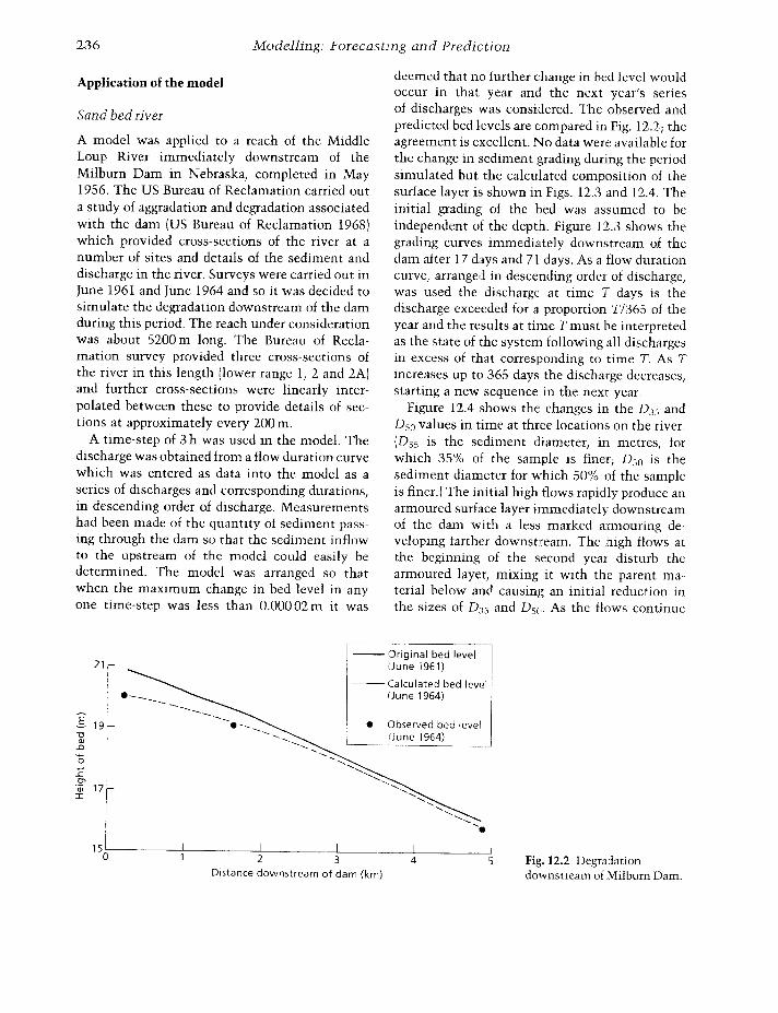
A model was applied to a reach of the MiddleLoup River immediately downstream of theMilburn Dam in Nebraska, completed in May1956. The US Bureau of Reclamation carried outa study of aggradation and degradation associatedwith the dam (US Bureau of Reclamation 1968)which provided cross-sections of the river at anumber of sites and details of the sediment anddischarge in the river. Surveys were carried out inJune 1961 and June 1964 and so it was decided tosimulate the degradation downstream of the damduring this period. The reach under considerationwas about 5200 m long. The Bureau of Reclamation survey provided three cross-sections ofthe river in this length (lower range 1, 2 and 2A)and further cross-sections were linearly interpolated between these to provide details of sections at approximately every 200 m.
A time-step of 3 h was used in the model. Thedischarge was obtained from a flow duration curvewhich was entered as data into the model as aseries of discharges and corresponding durations,in descending order of discharge. Measurementshad been made of the quantity of sediment passing through the dam so that the sediment inflowto the upstream of the model could easily bedetermined. The model was arranged so thatwhcn the maximum change in bed level in anyone time-step was less than 0.00002 m it was
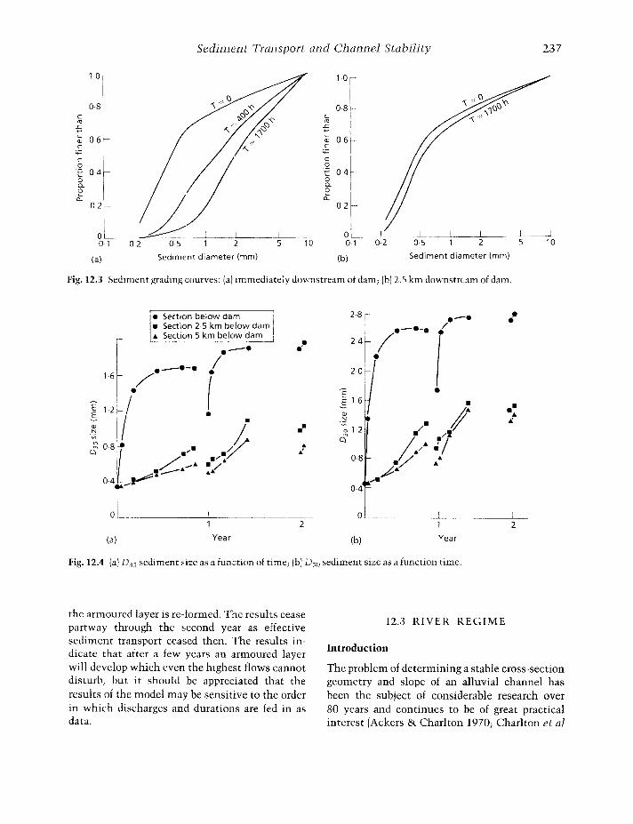
deemed that no further change in bed level wouldoccur in that year and the next year's seriesof discharges was considered. The observed andpredicted bed levels are compared in Fig. 12.2 i theagreement is excellent. No data were available forthe change in sediment grading during the periodsimulated but the calculated composition of thesurface layer is shown in Figs. 12.3 and 12.4. Theinitial grading of the bed was assumed to beindependent of the depth. Figure 12.3 shows thegrading curves immediate]y downstream of thedam after 17 days and 71 days. As a flow durationcurve, arranged in descending order of discharge,was used the discharge at time T days is thedischarge exceeded for a proportion T/365 of theyear and the results at time T must be interpretedas the state of the system following all dischargesin excess of that corresponding to time T. As Tincreases up to 365 days the discharge decreases,starting a new sequence in the next year.
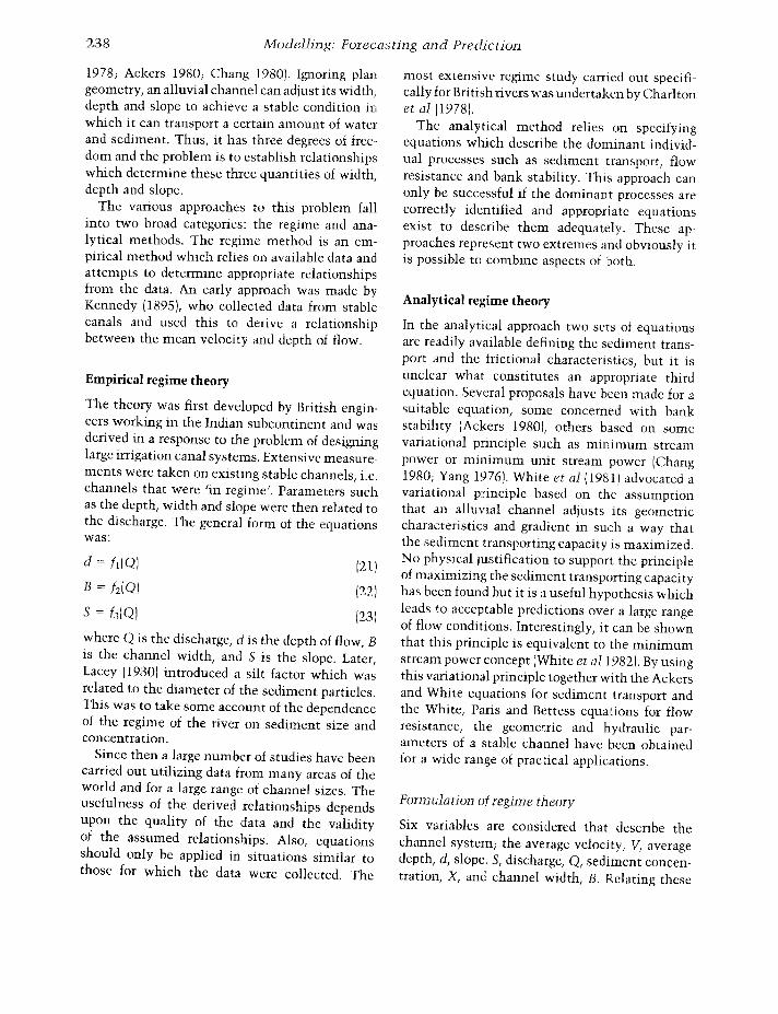
Figure l2.4shows the changes in the D3S andDso values in time at three locations on the river.(D35 is the sediment diameter, in metres, forwhich 35% of the sample is finer; Dso is thesediment diameter for which 50% of the sampleis finer.) The initial high flows rapidly produce anarmoured surface layer immediately downstreamof the dam with a less marked armouring developing farther downstream. The high flows atthe beginning of the second yeaI' disturb thearmoured layer, mixing it with the parent material below anJ causing an initial reduction inthe sizes of D35 and DSli. As the flows continue
--Original bed level(June i961)
--- Ca leu lated bed level(june 1964)
Fig. 12.2 Degradationdownstream of Milburn Dam.
_--,I~ -l4 52 3
Distance downstream of dam (km)
-------.-...... • Observed bed level
------ ......... _.. (June 1964)
....................................
...................
........ ,.............
..................
.....................................
......
21
.----I 19lJQ.I.0"+-0+'
..r::.O'l.~
1_I
150
Sediment Transport and Channel Stability 237
.~I I ~05 1 2 5 10
Sediment diameter (mm)
10
0·8cIII
-5(ij 06~.......c':2
04+-'
0I
D.-
e
°t0-
---'----~~ -~
5 10 0·1 0·2
(b)
2
SedimEnt diameter (mm)(a)
°1 L:k I Ia 1 02 05 1
~ 0.81l:+-'l..
WC~
Co
'-i=3oQ.
oCL
Fig. 12.3 Sediment grading <.:ourves: (al immediately downstream of dam; lh) 2.5 km downstrum of dam.
• Section below dam ]• Section 2·5 km below dam& Section 5 km below damI e_e
te_e-e!
16 /
E 12 i (0
j08l 0'· • .k/" ..... /
,~.-. ~/
04 .-1'
...-
.-••
28
2·4/e_e-.
e
.-eI'
re
~•
(a) Year
2a
(b)
~__ .__L.1
Year
. .. -----L-2
Fig. 12.4 (a) D35 sediment size as a function of time; (b) Dso sediment size as a function time.
the armoured layer is re-formed. The results ceasepartway through the second year as effectivesediment transport ceased then. The results indicate that after a few years an armoured layerwill develop which even the highest flows cannotdisturb, but it should be appreciated that theresults of the model may be sensitive to the orderin which discharges and durations are fed in asdata.
12.3 RIVER REGIME
Introduction
The problem of determining a stable cross-sectiongeometry and slope of an alluvial channel hasbeen the subject of considerable research over80 years and continues to be of great practicalinterest (Ackers & Charlton 1970; Charlton et a1
238 Modelling: Forecasting and Prediction
Empirical regime theory
The theory was first developed by British engineers working in the Indian subcontinent and wasderived in a response to the problem of designinglarge irrigation canal systems. Extensive measurements were taken on existing stable channels, i.e.channels that were 'in regime'. Parameters suchas the depth, width and slope were then related tothe discharge. The general form of the equationswas:
where Q is the discharge, d is the depth of flow, Bis the channel width, and S is the slope. Later,Lacey (1930) introduced a silt factor which wasrelated to the diameter of the sediment particles.This was to take some account of the dependenceof the regime of the river on sediment size andconcentration.
Since then a large number of studies have beencarried out utilizing data from many areas of theworld and for a large range of channel sizes. Theusefulness of the derived relationships dependsupon the quality of the data and the validityof the assumed relationships. Also, equationsshould only be applied in situations similar tothose for which the data were collected. The
1978; Ackers 1980; Chang 1980). Ignoring plangeometry, an alluvial channel can adjust its width"depth and slope to achieve a stable condition inwhich it can transport a certain amount of waterand sediment. Thus, it has three degrees of free··dom and the problem is to establish relationshipswhich determine these three quantities of widthidepth and slope.
The various approaches to this problem fallinto two broad categories: the regime and analytical methods. The regime method is an empirical method which relies on available data andattempts to determine appropriate relationshipsfrom the data. An early approach was made byKennedy (1895), who collected data from stablecanals and used this to derive a relationshipbetween the mean velocity and depth of flow.
d = idQl
B =h(Q)
s = f3(Q)
(21)
(22)
(23)
most extensive regime study carried out specifically for British rivers was undertaken by Charltonet al (1978).
The analytical method relies on specifyingequations which describe the dominant individual processes such as sediment transport, flowresistance and bank sta.bility. This approach canonly be successful if the dominant processes arecorrectly identified and appropriate equationsexist to describe them adequately. These approaches represent two extremes and obviously itis possible to combine aspects of both.
Analytical regime theory
In the analytical approach two sets of equationsarc readily available defining the sediment transport and the frictional characteristics1 but it isunclear what constitutes an appropriate thirdequation. Several proposals have been made for asuitable equation} some concerned with bankstability (Ackers 19801, others based on somevariational principle such as minimum streampower or minimum unit stream power (Chang1980; Yang 1976). White et al (1981) advocated avariational principle based on the assumptionthat an alluvial channel adjusts its geometriccharacteristics and gradient in such a way thatthe sediment transporting capacity is maximized.No physical justification to support the principleof maximizing the sediment transporting capacityhas been found but it is a useful hypothesis whichleads to acceptable predictions over a large rangeof flow conditions. InterestinglYi it can be shownthat this principle is equivalent to the minimumstream power concept (White et 011982). By usingthis variational principle together wi th the Ackersand White equations for sediment transport andthe White, Paris and Bettess equations for flowresistance, the geometric and hydraulic parameters of a stable channel have been obtainedfor a wide range of practical applications.
Formulation of regime theory
Six variables are considered that describe thechannel system; the average velocity: V, averagedepth} d, slope, 5, discharge, 0, sediment concentratioIl, Xi and channel width, B. Relating these
Sediment Transport and Channel Stability 239
variables are equations for the contmuity of waterflow, sediment transport formulas, tlow resistancefmmulas and the condition that the sedimenttransport should be maximized or, equivalently,stream power should be minimized. In the following treatment the discharge and slope areassumed to be imposed and the correspondingvalues of V d.. X and B are determined. Implicit inthis treatment are the assumptions that the flowis steady and uniform and that the bed and bankmaterial is non-cohesive.
Sediment transport. The Ackers and White (1973)equation has been used to calculate the sedimentconcentrations.
Frictional characteristics. By utilizing the samebasic parameters as in the Ackers and Whitesediment transport theory, White et a1 (1980)found that a linear relationship between the sediment mobility related to the total shear stress l
Ffg, in which:
(24)
(where V * is the shear velocity, D is the sedimentdiameter, s is the sediment specific gravity, andg is the acceleration due to gravity), and themobili ty, related to the effective shear stress, Fgr,
existed with coefficients depending on Dgf! thedimensionless sediment diameter. An extensivecorrelation for a wide range of sediment sizes10.4-10 mm) gave the equation:
~gr =1= 1.0 - 0.76[1 - (1 1D \1.71 (25)fg exp og grl
where A is the threshold of motion parameterin the Ackers and White sediment transporttheory. This method has been favourably compared with the traditional methods of Einsteinand Barbarossa (l952), Engelund (1966, 1967) andRaudkivi (1967) and showed good agreementwith data for sediment sizes in the range of 0.0468 mm (White et a1 1980).
Variational principle. One extra equadon wasneeded to solve the system. Various differentapproaches have been used to provide the necessary relationship, some of them relying on a type
of variational argument in which the maximumor minimum of some quantity is sought. Previousexperience led to the consideration of whetherthe system might maximize the sedimenttransporting capacity of the channel. Moreprecisely, the hypothesis is that, for a particularwater discharge and slope, the width of thechannel adjusts itself to maximize the sedimenttransport rate.
H one imposes values of discharge and slope butdoes not impose the condition of maximumsediment transport, then there arc a family ofsolutions each with different values of B, X, V andd, only one of which provides the maximumsediment transport rate. All the remaining solutions have sediment transport rates less thanthe maximum and widths both less than andgreater than that provided by the maximumtransport rate. These all represent possible solutions of the system if it is constrained in someway, for example by the relative erodibility of thebed and banks. Thus, a channel with banks whicharc less erodible than the bed will have a widthsmaller than that corresponding to the maximumsediment transport case, while a channel whosebanks arc more erodible than the bed will have awidth correspondingly larger.
While regime theory assumes that the flow isuniform and does not consider the plan geometryof the river, it has been suggested that a principleof maximum sediment transport capacity isinvolved in determining the plan shape of a river.Onishi et 01 (1976l claim that 'a meanderingchannel can be more efficient than a straight one,in the sense that a given water discharge cantransport a larger sediment load and, for somechannel configurations and flow conditions, canrequire a small energy gradient'. Thus, they postulate that the plan geometry of a river representsan attempt to maximize the transport rate. Thisshould also be considered when studying thecomparison of theory and observation for naturalrivers presented later. The effects of meanderingmay produce extremes different from those calculated on the basis of uniform flow.
Evaluation of regime theory
The method was compared with available data
240 Modelling: Forecasting and Prediction
and with existing empirical regime relationshipsderived by fitting curves to data. The field data forsand channels came from the Punjab canals.CHOP (Canals and Headworks Observation Program) canals, VP (Vttar Pradesh) and Sind Canals(ICID 1966), Pakistan canals (ACOP) (Mahmoodet al 1979b), and the Simons and Bender data forAmerican canals (Simons 1957). This provided atotal of 213 observations. The laboratory datawere taken from the work of Ackers (1964LAckers and Charlton (1970), and Ranga-Raju et al(1977). The present method was also comparedwith data from gravel rivers in Alberta fKellerhalset al 19721.
For comparison with observed data, calculations were performed in which observed valuesof Q and S were taken and the width, depthand sediment concentration calculated. For someof the data, a further calculation was performedin which observed values of Q and X were takenand the width, depth and slope were determined.For a fuller account of comparisons between observed and predicted data see White et al (1981).
For rivers, one has to select some dischargeas the dominant or significant discharge. In thepresent treatment this was arbitrarily chosen tobe the bankfull discharge. In considering theresults, it must be remembered that better agreement between prediction and observation mightbe obtained by a different choice of dominantdischarge.
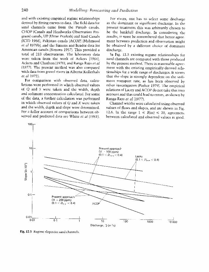
In Fig. 12.5 existing regime relationships forsand channels are comp.ared with those producedby the present method. There is reasonable agreement with the existing empirically-derived relationships for a wide range of discharges. It seemsthat the slope is strongly dependent on the sediment transport rate, as has been observed byother investigators (Parker 1979). The empiricalrelations of Lacey and ACOP do not take this intoaccount and this could lead to errors} as shown byRanga-Raju et al (19771.
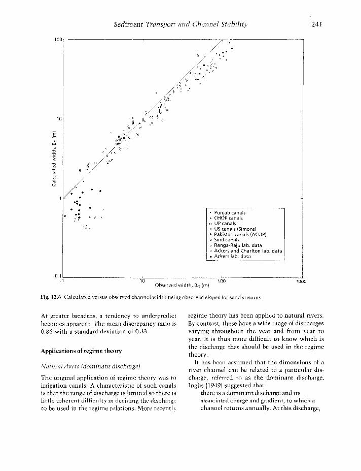
Channel widths were calculated using observedvalues of flows and slopes, and arc shown in Fig.12.6. In the range 1 ::s; Blm) :'E; 20, agreementbetween calculated and observed values is good.
100
10
Present approach(X 200 ppm)(0.1 < Dmm < 0.4)
...... _------
------~ ----J1000 10 000100
Present approach(X = 100 ppm)(0.1 < Dmm < 0.4)
10
Discharge, Q (mYs)
orO·OlL-__~__.L...1 ~_ .__
0·01 0-1 1
Fig. 12.5 Regime slopes for sand channels.
lOa,I
Sediment Transport and Channel Stability 241
10
• •• ••..••
• • •• ••
!.~>' 0
• Punjab canals" CHOP canalso UP canalso US canals (Simons).. Pakistan canals (ACOP)o Sind canals" Ranga-Raju lab. datat> Ackers and Charlton lab. data• Ackers lab. data
0.1~1------10
Observed width, Bo (m)100 1000
Fig. 12.6 Calculated versus observed channel width using observed slopes for sand streams.
At greater breadths, a tendency to underprcdictbecomes apparent. The mean discrepancy ratio is0.86 with a standard deviation of 0.33.
Applications of regime theory
Natural rivers (dominant discharge)
The original application of regime theory was toirrigation canals. A characteristic of such canalsis that the range of discharge is limited so there islittle inherent difficulty in deciding the dischargeto be used in the regime relations. More recently
regime theory has been applied to natural rivers.By contrast, these have a wide range of dischargesvarying throughout the year and from year toyear. It is thus more difficult to know which isthe discharge that should be used in the regimetheory.
It has been assumed that the dimensions of ariver channel can be related to a particular discharge, referred to as the dominant discharge.Inglis (19491 suggested that
there is a dominant discharge and itsassociated charge and gradient, to which achannel returns annually. At this discharge,
242 Modelling: Forecasting and Prediction
equilibrium is most closely approached andthe tendency to change is least. Thiscondition may be regarded as the integratedeffect of all varying conditions over a longperiod of time.
Unfortunately, there is no universally agreedmethod of determining the dominant discharge.
In a recent study a number of the differentdefinitions proposed for dominant discharge werecompared on data from large gravel rivers inAlberta. The data set was not extensive so it isdifficult to be dogmatic about the results, but thebest predicted expressions were those based onflow frequency. The discharge which is exceeded0.6% of the time gave the best predictions (Whiteet al 1986).
Design of physical models
As part of an investigation for a water intake foran irrigation scheme a mobile·bed model wasdesigned of the Sabi River} a large sand river inZimbabwe. The river channel was in regime andthe physical model was designed on the basis thatthe model channel must also be in regime (White1982). The resulting model successfully reproduced the behaviour of the prototype.
Assessment of morphological changes in rivers
An investigation was carried out into the impactof a proposed dam at Condo on the Sabi River.One of the effects of the dam would be to alter thedistribution of flows in the river downstream. Bydetermining how the dominant discharge wouldbe changed the effect that this would have onthe river morphology was assessed using regimetheory (Hydraulics Research 1982).
12.4 PLAN FORM OF RIVERS
Although the plan shapc of rivers displays acontinuous variation of form it has traditionallybeen classified into the three broad categories ofstraight, meandered or braided. The division intothe three categories is in part arbitrary as it isdifficult to distinguish between a straight channeland a meandering channel of low sinuosity andnot everybody agrees on what constitutes a mean-
dering or braided channel. There has been muchwork in the past to relate the shape and meanderpattern to variables such as the discharge and theslope. A successful method of predicting themeander geometry and the conditions for braid·ing would enable designs of alluvial channelsto be made with greater confidence and allow theprediction of the effects of engineering works on ariver system. At present, however} the predictionsthat can be made with confidence are few. Whatis presented here is not a definitive theory ofmeandering and braiding but rather a frameworkwithin which the problems of the meanderingand braiding of channels in equilibrium can beconsidered.
It is instructive to review some of the moresuccessful work that has been done on meandering and braiding. Leopold and Wolman (1957)plotted bankfull discharge against channel slopefor a number of natural channels. This indicatedthat in those rivers the braided channels wereseparated from the meandering channels by a linegiven by the equation:
S = 0.06 Q-0.44
where S is the slope, and Q is the discharge incusecs. The braided channels had steeper slopeswhile the meandered channels had smaller slopes.Leopold and Wolman took meandering to mean ariver with a sinuosity - the ratio of the thalweglength to the straight line distance - greaterthan 1.5. Their conclusions, however, were tentative as they pointed out that in natural channelsspecific variables often occur in association. Forexample, steep slopes are most frequently associated with coarse bed material. They also showedthat meander wavelength is related to the bankfull width of the channel and so they took it to beindirectly related to the bankfull discharge.
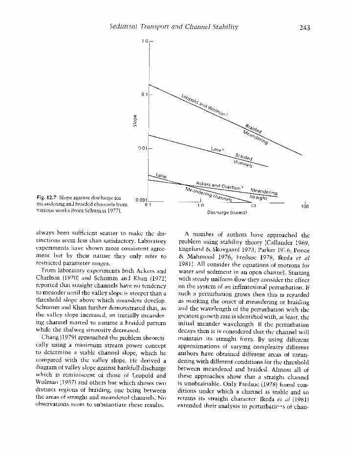
The approach of plotting slope against dischargehas also been used by others (Lane 1957; Ackers& Charlton 1979) and lines have been drawn onsuch plots to distinguish areas of braided, meandering and straight channels (Schumm 1977).There is, however} considerable variation between the lines (see Fig. 12.7). While the fieldevidence clearly shows that for a given dischargebraided channels are associated with the steepestslopes, meandering with the less steep andstraight rivers with the lowest slopes, there has
Sediment Transport and Channel Stability 243
Q.Ja...9.V'l
'T
01~
l0-01 ~-
Fig. 12.7 Slope against discharge for 0-001
meandering and braided channels from 0-1
various works Ifrom Schumm 19771.
always been sufficient scatter to make the distinctions seem less than satisfactory. Laboratoryexperiments have shown more consistent agreement but by their nature they only refer torestricted parameter ranges.
From laboratory experiments both Ackers andCharlton (1970) and Schumm and Khan (1972)reported that straight channels have no tendencyto meander until the valley slope is steeper than athreshold slope above which meanders develop.Schumm and Khan further demonstrated that, asthe valley slope increased, an initially meandering channel started to assume a braided patternwhile the thalweg sinuosity decreased.
Chang (1979) approached the problem theoretically using a minimum stream power conceptto determine a stable channel slope, which hecompared with the valley slope. He derived adiagram of valley slope against bankfull dischargewhich is reminiscent of those of Leopold andWolman (1957) and others but which shows twodistinct regions of braiding, one being betweenthe areas of straight and meandered channels. Noohservations seem to substantiate these results.
Discharge (cusecs)
A number of cmthors have approached theproblem using stability theory (Callander 1969;Engelund & Skovgaard 1973; Parker 19/6; Ponce& Mahmood 1976; Fredsoe 1978; Ikeda et al1981). All consider the equations of motions forwater and sediment in an open channel. Startingwith steady uniform flow they consider the effecton the system of an infinitesimal perturbation. Ifsuch a perturbation grows then this is rerardedas marking the onset of meandering or braidingand the wavelength of the perturbation with thegreatest glowth rate is identified with, at least, theinitial meander wavelength If the perturbationdecays then it is considered that the channel willmaintain its straight form. By using differentapproximations of varying complexity differentauthors have obtained different areas of meandering with different conditions for the thresholdbetween meandered and braided. Almost all ofthese approaches show that a straight channelis unobtainable. Only Fredsoe (1978) found conditions under which a channel is stable and soretains its straight character. Ikeda et a1 (1981)extended their analysis to perturbatiC'.....s of chan-

244 Modelling: Forecasting and Prediction
nels which were initially sinuous. None of thetheories adequately reproduces the sort of behaviour observed by Leopold and Wolman (1957)and others.
Theory of stable channel form
Bettess and White (1983) argued that it wouldseem that meandering and braiding are mechanisms by which the present conditions imposedon a river are reconciled with those conditionsnecessary to give a stable channel form. Thus it isnecessary to base the approach on the work doneon predicting stable channel forms. This has beendescribed above in the section on regime theory.In particular, it was indicated that, for a givensediment, a river carrying a particular dischargeand sediment load is stable only if the slope has aspecific value. In the following treatment theanalytical regime theory developed by White et al(1982) will be used but the essential ideas canbe incorporated with any well-founded regimetheory.
Application to meandering and braiding
The study of meandering and braiding of channelsin equilibrium can now be based on the beliefthat it arises because of a discrepancy betweenthe channel slope required for equilibrium andthe valley slope. There have been suggestionsthat if the channel slope required for equilibriumis less than the valley slope then the river systemmay accommodate this discrepancy by meandering. Less attention has been paid to the separation between meandering and braiding channels.In this approach a regime theory is used to determine the equilibrium river slope and by comparing this with the available valley slope it isdetermined whether the river will be straight,meandered or braided.
It is assumed that the discharge and the sediment concentration in the channel are fixed andthe regime theory may be used to determine thecorresponding equilibrium values of SRI, B, V andd, where SRI denotes the equilibrium slope (for asingle channel), B is the channel Width, V is thevelocity, and d is the depth of flow.
Given the valley slope, Sv, one can identify
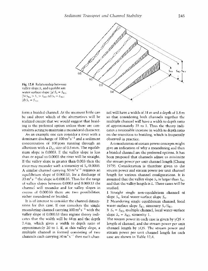
three different cases depending on the relativemagnitudes of SRI and Sv.1 If the valley slope, Sv, is equal to the riverslope then the channel will be straight and inequilibrium.2 If the valley slope is greater than the river slopethen the river can accommodate the discrepancyby meandering. Meandering reduces the slopemeasured along the channel in relation to theslope measured along the valley. Thus the channel slope may be reduced to SR 1 by the rivermeandering with a sinuosity of Sv/SR1' wheresinuosity is the ratio of the length betweentwo points measured along the channel to thatmeasured along the valley. The difference invalley and equilibrium slope can also be accommodated in another way, by the river braiding.Since/ if the sediment and sediment concentrationare kept fixed, the equilibrium slope is increasedby reducing the discharge by a factor of two, threeor more, the discrepancy between the valley andequilibrium slopes can be removed by the riveraltering from a single into a multiple channel.3 If the valley slope is less than the river slopethen the river cannot achieve the required equilibrium and alterations probably involving deposition or erosion of sediment will take placein order to bring about a different equilibriumcondition.Cases (1) and (21 are illustrated in Fig. 12.8.
The possibdity of the formation of multiplechannels is now considered in more detail. If itis assumed that the simplest form of multiplechannel is one approximating to two sub-channelseach carrying half the discharge then these channels will have some equilibrium slope SR2, andSR2 will be greater than SRI' More complex braidedchannels can be approximated by three or moresub-channels with equilibrium slopes SR3,SR4, ... , forming an increasing sequence ofnumbers.
For valley slopes less than SRI and above SRI,the only stable solution is for the channel tomeander with sinuosity Sy/SRI' If the valley slopeis equal to SR2 then there appears to be a cho:· eof solutions, either a meander channel withsinuosity Sv/SRI' or a straight double channel. Forvalley slopes m excess of SRI there appear to betwo possible solutions, either to meander or to
Sediment Transport and Channel Stability 245
Fig. 12.8 Relationship betweenvalley slope Sy and equilibnumwater surface slope: (a) Sy = SRli
Ib) S,u > Sy > 3Rli (c) Sy = SR2i
Id) Sy = S,o.
form a braided channel. At the moment little canbe said about which of the alternatives will berealized except that we would suggest that braiding is the preferred option unless there are constraints acting to maintain a meandered character.
As an example one can consider a river with adominant discharge of 100m3 s- 1 and a sedimentconcentration of 100ppm running through analluvium with a D35 size of 0.5 mm. The equilibrium slope is 0.0003. If the valley slope is lessthan or equal to 0.0003 the river will be straight.If the valley slope is greater than 0.003 then theriver may meander with a sinuosity of Sv/0.0003.A similar channel carrying 50 m3 s-1 requires anequilibrium slope of 0.000 33; for a discharge of33 m3 S--1 the slope is 0,()0035. Thus for the rangeof valley slopes between 0.0003 and 0.00033 thechannel will meander and for valley slopes inexcess of 0.000 33 there are two possibilities,either meandered or braided.
It is of interest to consider the channel dimensions for this case. If one considers the singlemeandering channel carrying 100 m3 s-1 with thevalley slope of 0.00033 then regime theory indicates that the width will be 44 m and the depth2.4 m, which gives a width to depth ratio ofapproximately 20 to 1. If, at this valley slope, amultiple channel is formed consisting of twochannels each carrying SO m 3
S-1 then each chan-
nel will have a width of 31 m and a depth of 1.8 mso that considering both channels together themultiple channel will have a width to depth ratioof approximately 35 to 1. Thus the theory indicates a noticeable increase in width to depth ratioon the transition to braiding, which is frequentlyobserved in practice.
A consideraton of stream power concepts mightgive an indication of why a meandering and thena braided channel are the preferred options. It hasbeen proposed that channels adjust to minimizethe stream power per unit channel length (Chang19791. Consideration is therefore given to thestream power and stream power per unit channellength for various channel configurations. It isassumed that the valley slope Sv is larger than SRI
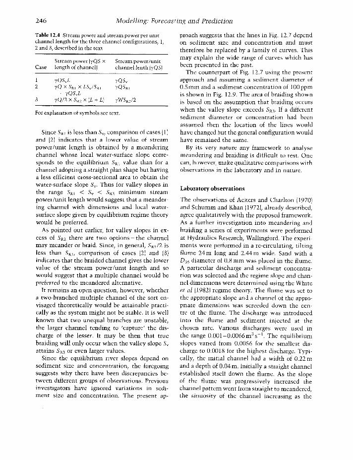
and that the valley length is L. Three cases will bestudied.1 Straight single non-equilibrium channel ofslope Sv, local water-surface slope Sv.2 Meandering single equilibrium channel, localwater-surface slope SR I, sinuosity SvlSRI'3 Sv = SR2, multiple chaIll1el, local water-surfaceslope Sv = SRI, sinuosity 1.The stream power in each case is given by yQS xlength of channel, and the stream power per unitchannel length by yQS. The stream power andstream power per unit channel length for eachcase are shown in Table 12.4.
246 Modelling: Forecasting and Prediction
Table 12.4 Stream power and stream power per unitchannel length for the three channel configurations, I,2 and 3, described in the text
Stream power [yQS X Stream power/unitCase length of channel) channellenth (yQS)
1 yQSvL yQSv2 yQ X SRI X LSjSRI yQSRI
= yQSvL
3 yQI2 X SR2 X (L + L) yWSR2 12
For explanation of symbols sec text.
Since SRI is less than Sy, comparison of cases (1)and (2) indicates that a lower value of streampower/unit length is obtained by a meanderingchannel whose local water-surface slope corresponds to the equilibrium SRi value than for achannel adopting a straight plan shape but havinga less efficient cross-sectional area to obtain thewater-surface slope Sv' Thus for valley slopes inthe range SRI < Sy < SR2 minimum streampower/unit length would suggest that a meandering channel with dimensions and local watersurface slope given by equilibrium regime theorywould be preferred.
As pointed out earlier! for valley slopes in excess of SR2 there are two options - the channelmay meander or braid. Since! in general, SR212 isless than SRi, comparison of cases (2) and (3)indicates that the braided channel gives the lowervalue of the stream power/unit length and sowould suggest that a multiple channel would bepreferred to the meandered alternative.
It remains an open question, however, whethera two-branched multiple channel of the sort envisaged theoretically would be attainable practically as the system might not be stable. It is wellknown that two unequal branches are unstable!the larger channel tending to 'capture' the discharge of the lesser. It may be then that truebraiding will only occur when the valley slope Svattains SR.3 or even larger values.
Since the equilibrium river slopes depend onsediment size and concentration, the foregoingsuggests why there have been discrepancies between different groups of observations. Previousinvestigators have ignored variations in sediment size and concentration. The present ap-
proach suggests that the lines in Fig. 12.7 dependon sediment size and concentration and musttherefore be replaced by a family of curves. Thismay explain the wide range of curves which hasbeen presented in the past.
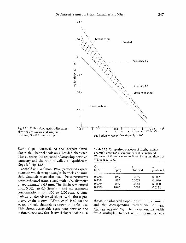
The counterpart of Fig. 12.7 using the presentapproach and assuming a sediment diameter of0.5mm and a sediment eoncentration of 100 ppmis shown in Fig. 12.9. The area of braiding shownis based on the assumption that braiding occurswhen the valley slope exceeds SR3' If a differentsediment diameter or concentration had beenassumed then the location of the lines wouldhave changed but the general configuration wouldhave remained the same.
By its very nature any framework to analysemeandering and braiding is difficult to test. Onecan, however, make qualitative comparisons withobservations in the laboratory and in nature.
Laboratory observations
The observations of Ackers and Charlton (1970)and Schumm and Khan (1972), already described!agree qualitatively with the proposed framework.As a further investigation into meandering andbraiding a series of experiments were performedat Hydraulics Research, Wallingford. The experiments were performed in a re-circulating, tiltingflume 24 m long and 2.44 ill wide. Sand with aD3S diameter of 0.8 mm was placed in the flume.A particular discharge and sediment concentration was selected and the regime slope and channel dimensions were determined using the Whiteel al (1982) regime theory. The flume was set tothe appropriate slope and a channel of the appropriate dimensions was screcded down the centre of the flume. The discharge was introducedinto the flume and sediment injected at thechosen rate. Various discharges were used inthe range O.OOl-O.0066m3 s- 1. The equilibriumslopes varied from 0.0056 for the smallest discharge to 0.0018 for the highest discharge. Typically, the initial channel had a width of 0.22 mand a depth of 0.04 m. Initially a straight channelestablished itself down the flume. As the slopeof the flume was progressively increased thechannel pattern went from straight to meandered,the sinuosity of the channel increasing as the
Sediment Transport and Channel Stability
0·8
247
Mo
x
0·7
06
04 -
0·3
Meandering
Non-equilibrium
Braided
-~--5inuosity1·2
'",--"--1----'',--- 5traig ht channel
Fig. 12.9 Valley slope against dischargeshowing areas of meandering andbraiding, D = O.S mm, X = ppm.
0.2 '-__ ,-----''-_ 1- I
0.6 0·5 1-0-4'- I 0·3 I I i 0·2 5E x 103
2 5 10 20 50 100 200 5001000 Q: m 3/s
Equilibrium water-surface slope, Sf x 103
flume slope mcreased. At the steepest flumeslopes the channel took on a braided character.This supports the proposed relationship betweensinuosity and the ratio of valley to equilibriumslope (d. Fig. 12.8).
Leopold and Wolman (19571 performed experiments in which straight single channels and multiple channels were obtained. The experimentswere performed using a sand with a D,,,") diameterof approximately 0.5 mm. The discharges rangedfrom 0.0024 to 0.0026m3 s- 1 and the sedimentconcentrations from 800 to 1800 ppm. A comparison of the observed slopes with those predicted by the theory of V\'hite et al (1982) for thestraight single channels 1S shown in Table 12.5.This shows reasonable agreement between theregime theory and the observed slopes. Table 12.6
Table 12.5 Comparison of slopes of single, straightchannels observed in experiments of Leopold andWolman (19571 and slopes predicted by regime theory ofWhite et al (1982)
Q X S S(m3 s- 1) (ppm' observed predicted
0.0024 865 0.0095 0.00820.0024 817 0.0079 0.00790.0024 830 0.0081 0.00800.0026 1840 0.0095 0.0122
shows the observed slopes for multiple channelsand the corresponding predictions for SRl,
SRI, SR3, SR4 and SR6' The corresponding widthfor a multiple channel with n branches was
248 Modelling: Forecasting and Prediction
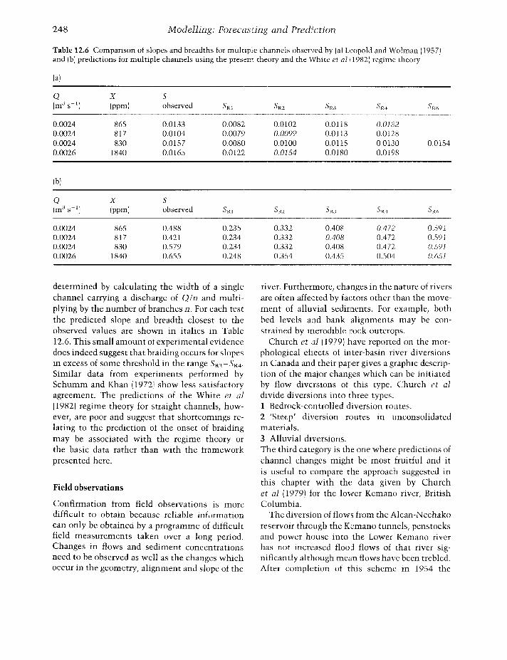
Table 12.6 Comparison of slopes and breadths for multiple channels observed by la) Leopold and Wolman (1957)and Ibl predictions for multiple channels using the present theory and the White et all1982l regime theory
(a)
Q X S(m" S-I) (ppml observed SRI SR2 SR:, SR4 SR()
0.0024 865 0.0133 0,0082, 0.0102 0.0118 0,01320.0024 817 0.0104 0.0079 0,0099 0.0113 0,01280.0024 830 0.0157 0.0080 0.0100 0,0115 0.0130 0.01540,0026 1840 0,0165 0.0122 0.0154 0,0180 0.0198
(bl
Q X S(m:' S-I) (ppm) observed SRI SR2 SR3 SR4 SR6
0.0024 865 0.488 0,235 0.:B2 0.408 0.472 0.S910.0024 817 0.421 0,234 0.332 0,408 0.472 0.5910.0024 830 0.579 0.234 0.332 0.408 0.472 0.5910.0026 1840 0.655 0.248 0.3.')4 0.435 0.504 0,651
determined by calculating the width of a singlechannel carrying a discharge of Q/n and multiplying by the number of branches 11. For each testthe predicted slope and breadth closest to theobserved values are shown in italics in Table12.6. This small amount of experimental evidencedoes indeed suggest that braiding occurs for slopesin excess of some threshold in the range SR2 - SR4.
Similar data from experiments performed bySchumm and Khan (19721 show less satisfactoryagreement. The predictions of the White et al(1982) regime theory for straight channels, however, are poor and suggest that shortcomings relating to the prediction of the onset of braidingmay be associated with the regime theory orthe basic data rather than with the frameworkpresented here.
Field observations
Confirmation from field observations is moredifficult to obtain because reliable infurmationcan only be obtainea by a programme of difficultfield measurements taken over a long period,Changes in flows and sediment concentrationsneed to be observed as well as the changes whichoccur in the geometry, alignment and slope of the
river. Furthermore, changes in the nature of riversare often affected by factors other than the movement of alluvial sediments. For example, bothbed levels and bank alignments may be constrained by inerodible rock outcrops.
Church et al (1979) have reported on the morphological eHects of inter-basin river diversionsin Canada and their paper gives a graphic description of the major changes which can be initiatedby flow diversions of this type. Church et aldivide diversions into three types.1 Bedrock-controlled diversion routes.2 'Stet-p' diversion routes in unconsolidatedmaterials.3 Allllvial diversions.The third category is the one where predictions ofchannel changes might be most frUitful and itis useful to compare the approach suggested inthis chapter with the data given by Churchet al (1979) for the lower Kemano river, BritishColumbia.
The diversion of flows from the Alcan-Nechakoreservoir through the Kemano tUllllels, penstocksand power house into the Lower Kemano riverhas not increased flood flows of that river significantly although mean flows have been trebled.After completion of this scheme in 1954 the
Sedinlent Transport and Channel Stability 249
channel has become wider. It was still a braidedchannel in 1975 but the sinuosity was somewhatless than in 1954. The pre-1954 mean flow in theriver was 42m3 s- 1 and the post-1954 mean flowhas been 136 m3 S-1.
If it is assumed that the diverted flow is relatively free of coarse sediment then mean flowswere increased by a factor of three and meansediment concentration5 were decreased by asimilar amount. Data presented by White et al(1982) suggest that the 'new' channel, once it hasreached equilibrium, should be wider and of alower slope. The effect of increasing the discharge alone would be tD produce a new widthapproximately 1.8 times the old width and a newslope approximately 0.75 times the old slope. Theeffect of decreasing the :;ediment concentrationalone would be to produce a new width approximately 0.9 times the old width and a new slopeapproximately 0.7 times the old slope. The combined effect is thus likely to increase widths by afactor of around 1.4 and decrease the equilibriumslope by a factor of around 104. Changes in widtharc likcly to occur far more quickly than changesin slope because the amount of sediment whichmust be transported to achieve the latter is ordersof magnitude higher than that required for theformer.
The original mean width of the Lower Kemanoriver was 288 m and hence the present approachsuggests a new equilibrium width of 400m. Thiscompares with the 1975 mean width of 370m.The braided channel noted in 1954 suggests that,at that time, the equilibrium slope of the channelwas significantly lower than the valley slope. Theprediction for the post-1954 flow conditions is fora decrease in the equilibrium slope which willincrease the difference between equilibrium andvalley slopes. Hence the main trend in the nextfew decades will be for the channel to becomemore braided. This is already apparent in thelower rcachcs of this partIcular river. In the longerterm degradation in the upper reaches and deposition in the lower reache~. will tend to reduce thevalley slope towards the predicted equilibriumslope. There is some eVldence that this processhas already started but the establishment ofa new equilibrium will probably take severalhundred years.
12.5 STABILITY AND INSTABILITY
Stability and instability within river systems andthe related topic of thresholds have long beendebated. This discussion has frequently been confused and contradictory because different notionsor definitions of stability have been adopted. Inthis account a particular definition of stabilitywill be adopted and the discussion will take placewithin this context. The reader is warned that theauthor's ideas on stability are personal and, somewould think, idiosyncratic.
Definitions of stability
As the initial definitions of stability arose inconnection with mechanical systems, these willfirst be reviewed and then the application of theseideas to river systems will be discussed.
Everybody has some intuitive idea of the concepts to which the word~ 'stable' apd 'unstable'refer. In the context of mechanics, if one alters adynamical system slightly, then, depending uponwhether this alteration subsequently has a smallor large effect on the system, one calls that systemstable or unstable.
The state of a physical system is described by anumber of quantities, such as coordinates, whichare a function of time. The number of such coordinates, and consequently the dimension ofthe motion, depend upon the particular stabilityproblem being considered. A motion can be seenas the trajectory of a point in a suitable space. Fora finite dimensional system the space Rn isalmost invariably used, and for an infinite dimensional system some function space will, in general, be needed. Suppose we have some motioncP(t) whose stability we wish to consider. Then wemust study a general class of motions uft) evolvingfrom initial conditions that are close, in someappropriate sense, to those for cPo The motion cPis stable if, by making u sufficiently close to 4>initially, u remains close for all subsequent time.
It will be noticed that in the above we referredto two functions being 'close' so, for a discussionof stability, it is necessary to introduce the ideaof nearness. Thus a distance function or metricmust be introduced which represents how closeor far apart two functions or points are. This
250 Modelling: Forecasting and Prediction
distance between two functions f and g is denotedby dU] g).
Liapunov formulated a definition of stabilityin the context of a system defined by a finitenumber of ordinary differential equations (Hahn19631. This has since been generalized to theinfinite dimensional case (Zubov 1964). A motion¢ is said to be stable if dl¢(t), u(t)) can be keptsmall be selecting the initial condition u(O) to besufficiently close to ¢(Ol. (It may be noted thatthe metric selected forms an integral part of thedefinition of stability.)
A motion is asymptotically stable with respectto a set M if the motion is stable and d¢(tl] u(t) * *
oas t* * ?? for all u such that u(O)?? M. Thus] anequilibrium is asymptotically stable if after aperturbation the system returns to the originalequilibrium state. If the system always returns tothe original equilibrium] independent of the sizeof the perturbation then the system is globallyasymptotically stable. If the system returns to theoriginal equilibrium only for perturbations of lessthan a particular size then the equilibrium isstable to perturbations of that size. An example ofsuch a form of stable equilibrium is a ball rollingin a basin. When the ball is at the lowest part ofthe basin it is stable. If the basin is infinite inextent then the system is asymptotically stable]since when perturbed the ball will always eventually return to the lowest point. If the basin isfinite in extent then the equilibrium is asymptotically stable only for those perturbations withinthe bowl. For larger perturbations the ball will nolonger return to the original equilibrium. Thedivision between perturbations for which the system will return to the original equilibrium andthose for which it does not could be regarded asforming some form of threshold.
Stability of channel shape
The above ideas have an obvious application tochannel stability. The equilibrium channel sizeand shape is normally indicated by regime theory.The perturbations to this equilibrium are normally caused by changes in the discharge] although human intervention can also be a sourceof perturbation. The basis of regime theory is that
although the channel size and shape may vary asthe flow varies, they will always tend to revertto the regime conditions. This represents a system that is asymptomatically stable to all sizes ofperturbation.
Stability of planform
To discuss planform stability one needs a moresophisticated approach to the definition of closeness. In the case of a ball rolling in a basin thenotion of the distance of the ball from the equilibrium is easy to grasp and to quantify. If one isto consider wave motions one has to be moresophisticated. The problem arises that two waveforms, or meandering river planforms] may beidentical in shape but merely translated relativeto each other. Using the normal metrics theseplanforms would be regarded as being a long distance apart, but in morphological terms we wouldnormally think of them as being identical. Muchwork has been done on the stability of waveforms(Benjamin 19721 and many of the concepts developed in that area can usefully be applied to riversoMost waves naturally progress introducing thenotion that, for the purposes of a stability analysis] two waves may be close to each other if theyhave the same shape even though the crests mayhave very different locations. Benjamin imposeda metric on the equivalence classes of waveforms]where each equivalence class consisted of translations of the same form. Thus if one wave orplanform is just a translation of the other thenthe 'distance' between them is zero. If the profilesof two waves or planforrns are very similar exceptfor a translation then they are considered tobe close. This is formally described as orbitalstability.
As hinted at above, this approach has an application to meandering channels. There is a naturaltendency for the planform of meandering channels to migrate downstream. If the planform remains constant subject to a translation then thesystem remains within the same equivalenceclass. If the planform is perturbed but the development of the meander pattern remains similarto that which would have occurred with theunperturbed form] subject to an arbitrary translation] then the system is stable. It can readily be
Sediment Transport and Channel Stability 251
seen that with this definition most meanderingor straight channels are stable.
Stability of braided channels
The problem of defining a metric on a braidedsystem presents more problems than for a meandering system. Braided channels normally displayrapid changes in the size, location and alignment of individual anabranches. But, in a similarfashion to the wave case discussed above, thecharacter of the river, in terms of the numberand size of the anabranches, normally remainsremarkably constant. A definition of stabilityshould, therefore, concentrate on the essentialfeatures rather than the rapid, cosmetic changesthat occur over a short time-scale but which leavethe nature of the channel unchanged. Howard etai (1970) showed how the topology of a braidedriver can be described independently of the preciselocations of the anabranches. Stability can thenbe defined in terms of a metric imposed on thesetopological variables. Using this approach it isfound that the majority of braided systems arestable.
Nature of perturbations
In considering the stability and instability of riversystems it is worth contemplating the natureof the perturbations that are imposed on thesystem. These can be natural, for example a largereturn-period flood event or a volcano suddenlyincreasing the sediment load substantially, orhuman-induced, for example the construction ofa dam. Most river systems are stable to smallperturbations. Thus, after a small flood or minorchange, a river system normally returns towardsits original state. An exception is in very flat ordeltaic regions. In such areas river channels cansuddenly shift from one course to another duringa modest flood. To return to the analogy of a ballrolling in a basin, the situation in these flat ordeltaic regions is equivalent to a ball rolling on agently undulating table. A small perturbation,equivalent in the river system to a small flood,is sufficient to move the ball from one localminimum to ~m adjacent one, or to shift thechannel from one course to another. It can be
noted that this also explains the ease with whichchanges occur in a braided system.
Most rivers demonstrate a remarkable abilityto recover from large perturbations. There aremany cases where, despite major changes inchannel size and shape occurring during a majorflood, the river has returned to its pre-flood condition within a few years. In terms of the definitions above this would be described as beingasymptotically stable. This asymptotic stabilityis frequently the cause of frustration to riverengineers. There have been many cases of engineering works being carried out to change eitherthe size or planform of rivers only for the river torevert back to its previous form in a few years.
In considering perturbations a distinction hasto be made, however, between rivers which arein equilibrium and, after a perturbation, returntowards the original equilibrium and rivers whicharc in transition due to changes in the externallyimposed variables} such as discharge. In this latter case the effect of a large perturbation may beto speed up or slow down the rate of change andthe river may never return towards its originalequilibrium.
12.6 FUTURE TRENDS
In predicting sediment transport there seems tobe two main avenues of current research. Topredict sand transport, efforts are being made tocombine predicted velocity and sediment concentration profiles together with bed load formulae to provide detailed sediment transportformulae. This generation of predictors are likelyto be sufficiently complicated that a computer ofsome sort will be needed to evaluate them. Theother avenue is studying the transport of gradedsediments and discovering more about hidingfunctions and how sediment sizes interact.
Numerical morphological modelling is alsoprogressing in two different directions. Effort isgoing into the development of two-dimensionalsediment transport models to predict transverseas well as longitudinal variations in bed level.Meanwhile attempts are being made to includebank processes in one-dimensional models sothat changes in channel width may be predicted.No doubt these same processes will eventually be
252 Modelling: Forecasting and Prediction
included in two- and three-dimensional numerical models.
The trends in work on planform appear to beless definite. In the past stability analyses havebeen carried out to attempt to predict channelform but the results of many of these have beenunconvincing. At present, much effort is beingexpended on collecting field data but with thepresent lack of appreciation of the mechanicsinvolved in the various processes, it seems un··likely that much of great value will emerge.
REFERENCES
Ackers P. (19641 Experiments on small streams inalluvium. Journal of Hydraulics Division, ASCB90(HY4) 1-38. [12.3]
Ackers P. (1980) Use of sediment transport concepts instable channel design. International Workshop onAlluvial River Problems, ROOTkee, India. [12.3]
Ackers P, Charlton FG. (19701 The geometry of smallmeandering channels. Proceedings of the Institute ofCivil Engineers Supp!. XII, Paper 73285. [12.3, 12.41
Ackcrs P, Charlton FG. (1979) The slope and resistanceof small meandering channels. Proceedings of thelnstitute of Civil Engineers Suppl. IS, Paper 7362 S.[12.5J
Ackers P, White WR. (1973) Sediment transport: newapproach and analysis. TournaI of Hydraulics Division, ASCE 99(HYll): 2041-60. [12.1 , 12.2,12.31
Benjamin TB. (1972) The stability of solitary waves.Proceedings 0/ the Royal Society, London, A 328:153-83. [12.5]
Bettess R, White WR. (1983l Meandering and braidingof alluvial channels. Proceedings of the Institute ofCivil Engineers Part 2, 75: 525-38. [12.5]
Brownlie WR. 11981) Prediction of Flow Depth andSediment Discharge in Open Channels. CaliforniaInstitute of Technology W M Keck. Lab., Report KHR-43A. [12.1]
Callander RA. (1969) Instability and river channels.Journal of Fluid Mechanics 36(3): 465-80. [12.4]
Chang HH. (1979) Minimum stream power and riverchannel patterns. Journal of Hydrology 41: 303-27.[12.4]
Chang HH. 119801 Stable alluvial canal design. Journalof Hydraulics Division, ASCE I06(HY5): 873-9].[12.3]
Charlton FG, Brown PM, Benson RW. (1978) The Hydraulic Geometry of Some Gravel Rivers in Britain,Report IT 180, Hydraulics Research, Wallingford, UK.[12.3]
Chollet JP, Cunge JA. /1980) Simulation of unsteadyflow in an alluvial stream. Applied MathematicalModelling 4(August): 234-44. [12.2J
Chow VT. (1959) Open Crmnel Hydmulics. McGrawHill, New York. [12.2]
Church M, Davies LB, Hellerhals R. (19791 Morphological effects of interbasin river diversions. CanadianJournal of Civil Engineering 6(]): 8-3. [] 2.4]
Cole CV, Tarapore ZS, Dixit JG. (1973) Applicability ofsediment transport formulae to natural streams.Proceedings of the 15th lAHR Congress, Istanbul,1973, vol. I, Paper A53. [12.1]
De Vries M. (1976) Morphological Computations. DelftUniversity of Technology. [12.21
Einstein HA, Barbarossa NL. 119521 River channelTOughness. Transactions of the ASCE, 117: 1121-76.[12,3]
Engelund F. I] 966l Hydraulic resistance of alluvialstreams, JHD. Proceedings of the ASCE 92(HY2):315-26.[12.31
Engelund F. (1967) Proceedings of the ASCE 93(HY4):287-96. [12.3]
Engelund F, Skovgaard D. (1973) On the origin of meandering and braiding in alluvial streams. Journal ofFluid Mechanics 57(2): 289-302. [12.4]
Frcdsoe J. (1978) Meandering and braiding of riverslonrnal of Fluid Mechgnics 84(41: 609-24. [12.4]
Garde RJ, Ranga Raju KG. (1985) Mechanics of sediment transportation and alluvial stream problems,2nd edn. John Wiley, Chichester. 112.1]
Hahn W. (1963) Theory and Application of Liapunov'sDirect Method. Prentice-Hall, New York. [12.5]
Howard AD, Keerch ME, Vincent CL. (19701 Topologicaland geomctical properties of braided streams. WaterRe80urces Research 6(6): 1674--88. [12.5]
Hydraulics Research. (1982) Sobi River, Zimbabwe,Sedimentation Studies. Report EX 1020, HydraulicsResearch, Wallingford, UK. [12.3]
Ikeda S, Parker G, Sawai K. (1981) Bend theory of rivermeanders: Part 1 Lincardeve1opment. T01.lInal of FluidMechanics 112: 363~ 77. [12.4]
Inglis Cc. (1949) The Behaviour and Control of Riversand Canals. Research Publication No. 13, CentralBoard Inigation India, Simla. [12.3]
Kellerhals R, Neill CR, Bray DJ. (1972) Hydraulic andGeomorphic Characteristics of Rivers in Alberta.Report 72-1, Rivcr Engineering and Surface Hydrology,Research Council of Alberta, Alberta, Canada. 112.3]
Kennedy RG. (1895) On the prevention of silting inirrigation channels. Proceedings of the Institute ofCivil Engineers 119. 112.3]
Lacey G. (1930) Stable channels in alluvium. Proceedings of the Institute of Civil Engineers 229: 259-384.[12.3]
Lane EW. (1957) A Study of the Shape of ChannelsFormed by Natural Streams Flowing in ErodibleMaterial. US Army Engineering Division, MissouriRiver, Corps Engineers, MRD, Sediment Series 9.[12.4]
Leopold LB, Wolman MG. (1957) River channel pat-
Sediment Transport and Channel Stability 253
terns: braided, meandering and straight. US Geological Survey, Professional Paper, pp. 282-8. [12.4]
Mahmood K et a1. (1979a) Selected Equilibrium StateData fwm ACOP Canals. Report EWR 79.2, Civil,Mechanical and Environmental Engineering Dept.,George Washington University, Washington, DC.[12.3]
Mahmood K, Tarar RN, Masood T. (1979b) HydraulicGeometry Relations for ACOP Canals. Report EWR79.3, Civil, Mechanical and Environmental Engineering Dept., George Washington UniverSity,Washington DC. [12.3]
Onishi Y, Jain SC, Kennedy JF. (1976) Effects of meandering in alluvial streams. Tournal 0/ the HydraulicsDivision, ASCE IOZjHY7: 899-917. [12.3]
Parker G. (1976) On the cause and characteristic scalesof meandering and braiding in rivers. Tournal of FluidMechanics 76(3): 457-80 [12.4]
Parker G. (1979j Hydraulics geometry of active gravelrivers. TournaI of the HydraUlics Division, ASCEI05(HYQI: 1185-201. [12.3J
Ponce VM, Mahmood K. (1976) Meandering thaIwegs instraight alluvial channels. In: Rivers '76: Symposiumon Inland Waterways for Navigation, Flood Controland Water Diversions, pp. 1418---41. ASCE, FortCollins, USA. [12.4]
Ponce VM, Garcia JL, Simons DB. 119791 Modellingalluvial channel bed transients. lournal of theHydraulics Division, ASCE 105(HY3): 245-56.
Ranga-Raju KG, Dhandapani KR, Kandop DM. (1977)Effect of sediment load on stable sand canaldimensions. lournal of Waterway, Port, Coastal andOcean Division, ASCE I03(WW21: 241-9. [12.31
Raudkivi AT. (1990) Loose Boundary Hydraulics, 3rdedn. Pergamon Press, Oxford. [12.11
Schumm SA. 119771 The Fluvial System. John Wiley,New York. [12.4]
Schumm SA, Khan HR. (19721 Experimental studyof channel patterns. Geological Society of AmericaBulletin 83: 1755-70. [12.41
Shields A. (1936) Anwendung der Aelinlichkeits. mechanik und der turbulcnz forschung auf die Gcschiebebewegung. Mitteilungen der pruessischenverSllchsanstalt fur wass'!-rball llnd schiffbau, Berlin.[12.1 ]
Simons DB. (1957) Theory and design of stable channelsin alluvial material. PhD thesis, Colorado State University Fort Collins. [12.:3]
Task Committee on Preparation of Sediment Manual.(1971) Sediment transportation mechanics: sedimentdischarge formulae. 10llInal of the Hydraulics Division, ASCE 97(HY4): 523-67. [12.1]
US Army Corps of Engineers. (1976) Scour and deposition in rivers and reservoirs: computer program HEC-6. Hydrologic Engineering Centre, Davis, California.[12.21
US Bureau of Reclamation (1968) Behaviour of MiddleLoup River Channel as Influenced by Milburn Diversion Dam. US Department of Interior, SedimentationBranch, Denver, Colorado. [12.2]
Van Rijn LC.11984a) Sediment transport Part I: Bed loadtransport. TournaI of Hydraulic Engineering, ASCE110: 1431-56. [12.4]
Van Rijn LC. (1984b) Sediment transport Part II: Suspended load transport. TournaI of Hydraulic Engineering, ASCE 110: 1613-41. [12.41
White WR. (1982) A novel loose boundary model forinvestigating sedimentation problems at an intake.In: International Conference on Hydraulic Modellingof Civil Engineering Structures, Coventry, England,pp. 181-94. BHRA. [12.3]
White WR, Day TJ. (1980) Sediment transport in gravelbed rivers. In: Hey RD, Bathurst JC, Thorne CR (cds)Gravel Bed Rivers. Wiley, Chichester. [12.2]
White WR, Milli H, Crabbe AD. 119731 Sediment Transport: an Appraisal of Available Methods. Report INT119, Hydraulics Research Station, Wallingford. [12.2]
White WR, Paris E, Bettess R. (1980l The frictionalcharacteristics of alluvial streams: a new approach.Proceedings of the Institute of Civil Engineers Part 2,69: 737~50. [12.2, 12.3]
White WR, Paris £, Bettess R. (1981) River regime based011 sediment transport concepts. Report IT 201, Hydraulics Research, Wallingford. [12.3]
White WR, Bettess R, Paris E. (19821 Analytical approachto river regime. Journal of the Hydraulics Division,ASCE 108(HYlO): 1179-93. [12.3, 12.4]
White WR, Bettess R, Wang Shiqiang (19861 A studyon river regime. Report SR 89, Hydraulics Research,Wallingford, UK. [12.31
Yang CT. (1976) Minimum unit stream power andfluvial hydraulics. lournal of the Hydraulics Division, ASCE l02(HY7): 919-34. [12.31
Zubov VA. 11964) Methods of AM Lyapunov and TheirApplication. Noordhoff. [12.5]