Embed Size (px)
Citation preview
478 Finance a úvěr-Czech Journal of Economics and Finance, 66, 2016, no. 6
JEL classification: C32, C58, F51, G15 Keywords: “Systemic five”, Russian stock market, Ukrainian crisis, sanctions, return spillovers,
volatility spillovers, network dynamics, propagation value
The Russian Stock Market during the Ukrainian Crisis: A Network Perspective* Harald SCHMIDBAUER—BRU-IUL, ISCTE Business Research Unit, ISCTE-IUL, Lisboa
([email protected]), corresponding author Angi RÖSCH—FOM University of Applied Sciences, Munich, Germany Erhan ULUCEVIZ—Istanbul Kemerburgaz University, Istanbul, Turkey Narod ERKOL—Universitat Autònoma, Barcelona, Spain
Abstract The goal of the this paper is to investigate the shock spillover characteristics of the Russian stock market during different rounds of sanctions imposed as a reaction to Russia’s alleged role in the Ukrainian crisis. We consider six stock markets, represented by their respective stock indices, namely the US (DJIA), the UK (FTSE), the euro area (Euro Stoxx 50), Japan (Nikkei 225), China (SSE Composite) and Russia (RTS). Linking these markets together in a network on the basis of vector autoregressive processes, we can measure, among other things: (i) direct daily return and volatility spillovers from RTS to other market indices, (ii) daily propagation values quantifying the relative importance of the Russian stock market as a return or volatility shock propagator, and (iii) the amount of network repercussions after a shock. The last two are methodological innovations in this context. It turns out that distinct spillover patterns exist in different rounds of sanctions. Large-scale sanctions, beginning in July 2014, rendered the consequences of shocks from Russia less predictable. While these sanctions reduced the importance of the Russian stock market as a propagator of return shocks, they also increased its importance as a propa-gator of volatility shocks, thus making the network more vulnerable with respect to volatility shocks from the Russian stock market. This is a form of backlash that the sanc-tioning economies have been facing.
1. Introduction Russia’s economy is of relatively moderate size in terms of aggregate figures.
In 2013, Russia’s GDP was around 2.8% of global GDP; the total value of Russia’s stock market in 2012 was around 1.5% of the world stock market value.1 Russia’s trading volume with the EU was approximately EUR 340 billion at that time2 and the EU’s GDP was approximately EUR 13,500 billion.3 However, empirical studies have found evidence of strong dependence between Russia as one of the major raw-* The authors would like to thank two anonymous referees whose constructive criticism helped to improve
especially our explanations of the methodological foundations of the paper. 1 The authors’ own calculations based on data provided by the World Bank; see http://data.worldbank.org/data-catalog/GDP-ranking-table, http://data.worldbank.org/indicator/CM.MKT.TRAD.CD. Retrieved 2015-05-21. 2 “European Union, Trade in goods with Russia”, released by the European Commission; available online at http://trade.ec.europa.eu/doclib/docs/2006/september/tradoc_113440.pdf. Retrieved 2015-10-04. 3 Data retrieved 2015-10-04 from the Eurostat database; see http://ec.europa.eu/eurostat/tgm/refreshTableAction.do?tab=table&plugin=1&pcode=tec00001&language=en.
Finance a úvěr-Czech Journal of Economics and Finance, 66, 2016, no. 6 479
materials exporter along with its fellow BRIC (Brazil, Russia, India, China) country Brazil and the US markets, as well as a significant increase of connectedness among BRIC equity markets and with equity markets in the developed world beginning in 2005 (see Alou et al., 2011; Schmidbauer et al., 2013a). Bekiros (2014), investi-gating the spillover effects of the US financial crisis to the BRIC markets, also finds that “[...] almost all markets have become more internationally integrated after the US financial crisis and the consequent Eurozone sovereign debt crisis”.
1.1 Are Sanctions against Russia a Source of Financial Trouble? The recent sanctions against Russia, starting in March 2014, for its alleged
role in the Ukrainian crisis and annexation of Crimea (a chronology of events and sanctions will be given in more detail in Section 2), may have contributed to struc-tural changes of Russian interconnectedness.
Due to the sanctions, Russian companies faced difficulty rolling over debts from Western financial markets.4 The oil price drop from USD 100 (in June 2014) to USD 60 (in December 2014) further aggravated the situation, distorting the Russian budget balance and weakening the Russian economy significantly. As a result, com-panies’ demand for dollars increased, followed by demand from Russian consumers. This initiated a vast ruble devaluation and forced the Central Bank of Russia to increase interest rates from 10.5% to 17% in December 2014.5
There were fears that the ruble’s devaluation could have adverse effects on the global economy, as had been experienced during the 1998 Russian crisis. Blanchard and Arezki of the IMF also warned of the possible side effects of the Russian crisis.6 On the other hand, there were views suggesting that the likelihood of such a contagion effect had decreased:7 “One major difference between 1998 and today is that tough sanctions on Moscow have somewhat insulated Western investors from what’s ailing Russia.” According to this source, Michael Levi, a senior fellow at the Council on Foreign Relations, stated that “the sanctions regime has reduced the risk of financial contagion considerably. This is not 1998. You don’t have the same level of interconnectedness.”
1.2 Crises Changing Economic Paradigms: Contagion and Spillovers The first chapter of a book by Claessens and Forbes (2001) begins with
the following sentence: “Before 1997, the term ‘contagion’ usually referred to the spread
4 “Western sanctions and rising debts are already strangling the Russian economy”, Forbes, 2014-08-28; available online at http://www.forbes.com/sites/paulroderickgregory/2014/08/28/western-sanctions-and-rising-debts-are-already-strangling-the-russian-economy. Retrieved 2015-09-14. 5 “Russian central bank raises interest rate to 17% to prevent rouble’s collapse”, The Guardian, 2014-12-15;available online at http://www.theguardian.com/world/2014/dec/15/russia-interest-rate-rise-17pc-rouble-collapse-oil-price. Retrieved 2015-09-14. 6 “Oil prices have plunged recently [...] One of the lessons from the Great Financial Crisis is that large changes in prices and exchange rates, and the implied increased uncertainty about the position of some firms and some countries, can lead to increases in global risk aversion, with major implications for repricing of risk and for shifts in capital flows. This is all the more true when combined with other developments such as what is happening in Russia. One cannot completely dismiss this tail risk.”The Guardian, 2014-12-22; available online at http://www.inkl.com/news/trust-bank-becomes-first-financial-casualty-of-russia-s-currency-crisis. Retrieved 2015-09-14. 7 “Russian ruble crisis: Don’t panic like it’s 1998”, CNNMoney, 2014-12-17; available online at http://money.cnn.com/2014/12/17/investing/russia-crisis-1998-investing/. Retrieved 2015-05-27.
480 Finance a úvěr-Czech Journal of Economics and Finance, 66, 2016, no. 6
of a medical disease.” In the wake of Thailand’s 1997 and Russia’s 1998 currency devaluations affecting global financial markets, the notion of contagion entered mainstream economic terminology, prompting a series of academic investigations in the early 2000s (see Forbes, 2012), as well as sparking concerns among policy makers. In particular, the IMF (2008, 2011a) underlined the importance of inves-tigating financial sector spillovers, stating that “work on spillovers should continue, with modalities (e.g., frequency, coverage and context) that could evolve as expe-rience is gained with the exercise” (IMF, 2011a), and the IMF Spillover Reports (e.g. IMF, 2011b, 2012) assess the external effects of policies in five systemic economies: China, the euro area, Japan, the United Kingdom, and the United States.
There is no consensus either on the exact definition of contagion or on the methodology for quantifying it (for surveys of definitions, classifications and transmission channels of contagion, see Karolyi, 2003, and Dungey et al., 2005). According to the World Bank,8 “contagion is the cross-country transmission of shocks or general cross-country spillover effects”, which can take place both during “good” times and “bad” times. Gallo and Otranto (2008) discuss “spillover”, “contagion”, “interdependence” and “co-movement” concepts, which are often used synony-mously, on the basis of the relative role of one market to another and try to establish some practical definitions.
Similar to the contagion literature flourishing in the wake of the crises of the late 1990s, spillover literature was mainly triggered by the crash of global markets in October 1987. Early works on return and volatility spillovers go back to the seminal papers by Hamao et al. (1990), who analyze short-term price changes and price volatilities across global markets (Tokyo, London and New York), and, similarly, Engle et al. (1990), who utilize intraday returns to measure volatility transmissions from one period to the next within and across markets. King and Wadhani (1990) also provided one of the main works investigating the reasons underlying the simultaneous collapse of world markets following the October 1987 crash. Susmel and Engle (1994) analyze the return and volatility spillovers between the equity markets of New York and London.
Due to the increasing interest in the issue, the scope and breadth of works relating to it have been enlarged extensively: for detailed methodological surveys, see, for example, Claessens and Forbes (2001), Pericoli and Sbracia (2003), Karolyi (2003), Dungey et al. (2005) and Felipe and Diranzo (2006). Empirical applications also abound, covering a wide spectrum of countries, markets, assets, industries and the frequency of the data used.
1.3 Particular Studies in Contagion and Spillovers The October 1987 crisis mainly hit developed markets and, indeed, one strand
of literature investigates spillovers within developed economies. For example, Baur and Jung (2006) analyze return and volatility spillovers between the US and German stock markets using intraday data. Similarly, Dimpfl and Jung (2012) investigate the transmission of return and volatility spillovers around the world using data from the Euro Stoxx 50 (euro area), the S&P 500 (US) and the Nikkei 225 (Japan). Golosnoy
8 See http://go.worldbank.org/JIBDRK3YC0. Retrieved 2013-06-02.
Finance a úvěr-Czech Journal of Economics and Finance, 66, 2016, no. 6 481
et al. (2015) measure intradaily volatility spillovers before and during the subprime crisis within and across the US, German and Japanese stock markets.
However, crises originating from the emerging economies in the late 1990s shifted the focus to efforts to understand spillovers among developed and emerging economies. For example, Diebold and Yilmaz (2009) quantify return and volatility spillovers among 19 equity markets, which include developed and emerging economies. Bekiros (2014) investigates volatility spillovers among the US, EU and BRIC markets. Balli et al. (2015) analyze return and volatility spillovers from developed markets to selected emerging Asian countries and countries in the Middle East and North Africa region.
Shifting its focal point away from shocks and negative events, the notion of interdependence (or interconnectedness) covers a broader scope than contagion (Forbes, 2012), thus paving the way for the application of a wide variety of stochastic models. In this vein, globalization and the coupling of economies led to a prospering body of literature aiming to understand intra- and inter-regional return and volatility spillovers. Gallo and Otranto (2008), Engle et al. (2012), Baur (2003) and Yilmaz (2010) study the spillovers to and within selected Asian economies, whereas Gebka and Serwa (2007) investigate return and volatility spillovers between emerging markets in Central and Eastern Europe, Latin America and Southeast Asia.
Many researchers have zoomed in on the finer details of economies and markets with the purpose of focusing on understanding the spillover behavior between specific countries, markets, sectors and commodities, among other things. Diebold and Yilmaz (2014) track the connectedness of major US financial institu-tions’ stock return volatilities. Several papers tackle the analysis of return and vola-tility spillovers, among them Harris and Pisedtasalasai (2006), focusing on spillovers between large and small stocks in the UK; Choudhry and Jayasekera (2014), inves-tigating the impact of the 2008 global crisis on spillovers in the European banking industry; and Zhang and Wang (2014), analyzing spillovers between China, the world’s second-largest oil importer, and the world oil markets. Malik and Hammoudeh (2007) examine the volatility transmission between the oil market and the US, Bahraini, Kuwaiti and Saudi stock markets. Diebold and Yilmaz (2012) evaluate volatility spillovers among US stock, bond, foreign exchange and commodities markets. Hou (2013) addresses spillover effects from the short-term interest-rates market to equity markets within the euro area. Bubak et al. (2011) analyze volatility spillovers between Central European and EUR/USD foreign exchange markets. Adam et al. (2015) investigate linkages between international financial markets and Polish stock, bond and foreign exchange markets. Adam and Benecka (2013) trace the transmission of financial stress from the euro area to the Czech Republic.
There are also event studies elaborating the impact of certain events on other economic entities. For example, Gurgul and Wojtowicz (2015) study the impact of US macroeconomic data announcements on the prices of the most liquid shares of the Vienna Stock Exchange. This approach typically looks at markets in isolation and does not assume a network perspective and is thus of lesser relevance for the present study.
482 Finance a úvěr-Czech Journal of Economics and Finance, 66, 2016, no. 6
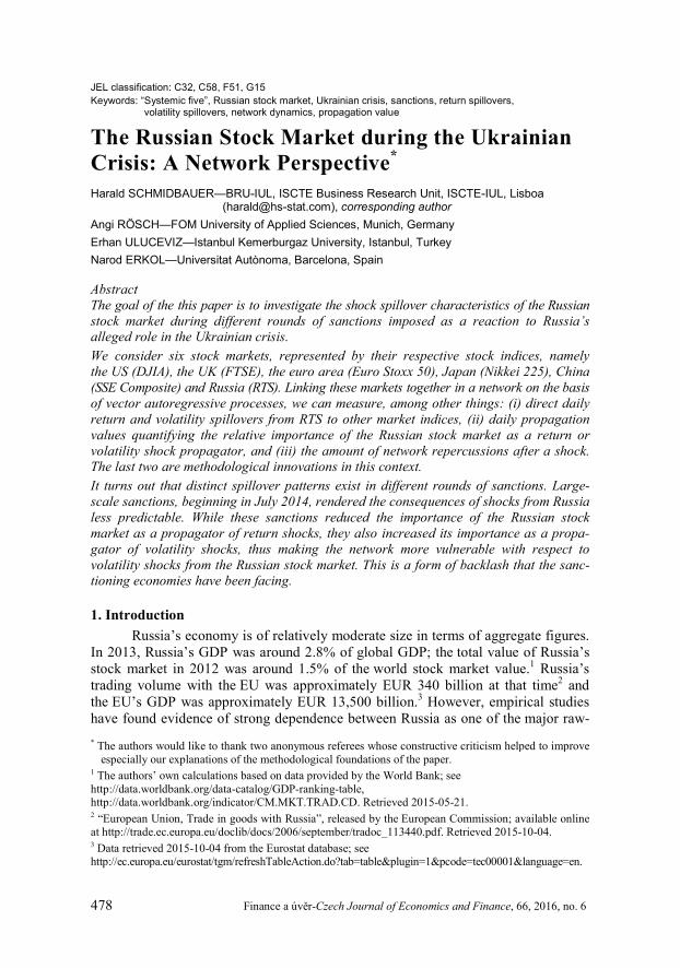
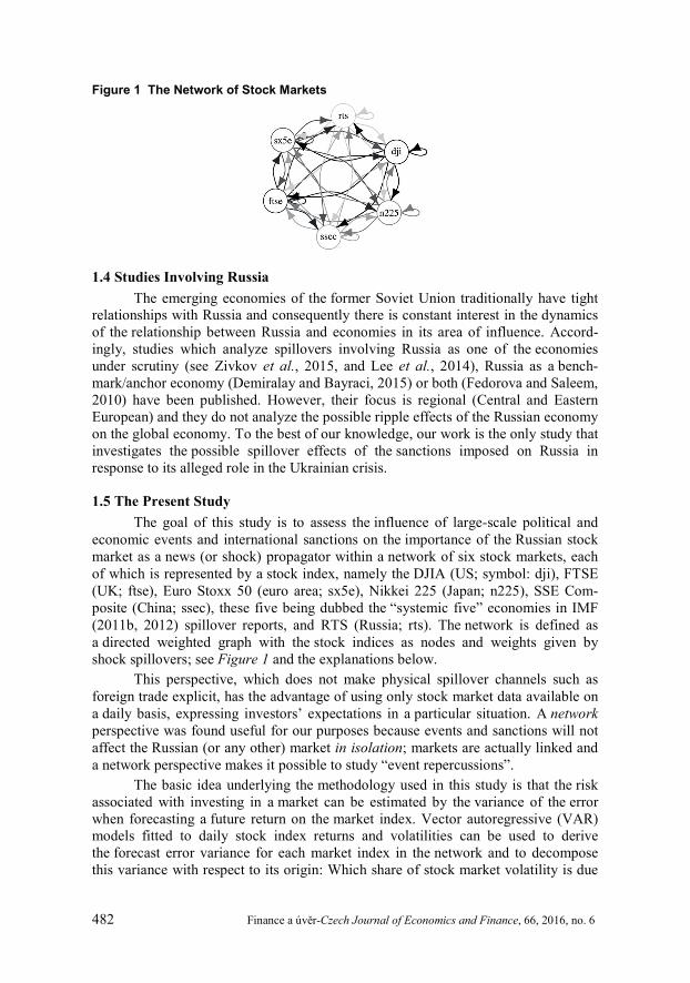
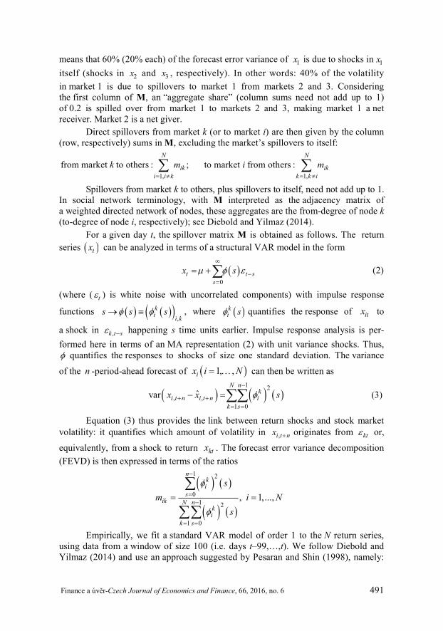
Figure 1 The Network of Stock Markets
1.4 Studies Involving Russia The emerging economies of the former Soviet Union traditionally have tight
relationships with Russia and consequently there is constant interest in the dynamics of the relationship between Russia and economies in its area of influence. Accord-ingly, studies which analyze spillovers involving Russia as one of the economies under scrutiny (see Zivkov et al., 2015, and Lee et al., 2014), Russia as a bench-mark/anchor economy (Demiralay and Bayraci, 2015) or both (Fedorova and Saleem, 2010) have been published. However, their focus is regional (Central and Eastern European) and they do not analyze the possible ripple effects of the Russian economy on the global economy. To the best of our knowledge, our work is the only study that investigates the possible spillover effects of the sanctions imposed on Russia in response to its alleged role in the Ukrainian crisis.
1.5 The Present Study The goal of this study is to assess the influence of large-scale political and
economic events and international sanctions on the importance of the Russian stock market as a news (or shock) propagator within a network of six stock markets, each of which is represented by a stock index, namely the DJIA (US; symbol: dji), FTSE (UK; ftse), Euro Stoxx 50 (euro area; sx5e), Nikkei 225 (Japan; n225), SSE Com-posite (China; ssec), these five being dubbed the “systemic five” economies in IMF (2011b, 2012) spillover reports, and RTS (Russia; rts). The network is defined as a directed weighted graph with the stock indices as nodes and weights given by shock spillovers; see Figure 1 and the explanations below.
This perspective, which does not make physical spillover channels such as foreign trade explicit, has the advantage of using only stock market data available on a daily basis, expressing investors’ expectations in a particular situation. A network perspective was found useful for our purposes because events and sanctions will not affect the Russian (or any other) market in isolation; markets are actually linked and a network perspective makes it possible to study “event repercussions”.
The basic idea underlying the methodology used in this study is that the risk associated with investing in a market can be estimated by the variance of the error when forecasting a future return on the market index. Vector autoregressive (VAR) models fitted to daily stock index returns and volatilities can be used to derive the forecast error variance for each market index in the network and to decompose this variance with respect to its origin: Which share of stock market volatility is due
Finance a úvěr-Czech Journal of Economics and Finance, 66, 2016, no. 6 483
to shocks in which other stock market? This approach provides a framework for dis-cussion of pairwise shock spillovers, arranged in a so-called spillover table, and was proposed by Diebold and Yilmaz (2009, 2012). The spillover table is interpreted as a network adjacency matrix (see Diebold and Yilmaz, 2014).
The spillover table is updated daily by fitting VAR models to a rolling window of return data. A VAR model can, in this sense, be adapted to measure return- and volatility-to-volatility spillovers in a network analysis. Schmidbauer et al. (2013b) discuss further aspects of spillover tables and show how to define the “propagation value” of a market, which can be interpreted as the relative impor-tance of a market as a news propagator; it measures an aspect of the centrality of the market in the network.
The methodology, as outlined, uses a VAR model in daily returns; it can thus assess daily return-to-volatility spillovers (for simplicity, called the ret2vol case in the following), i.e. it permits tracing the network consequences (in terms of return volatility) of a return shock to a market. Again, following Diebold and Yilmaz (2009), it is also possible to fit VAR models to daily return volatilities (instead of returns themselves) and proceed as before; this approach can quantify volatility-to-volatility spillovers (the vol2vol case), i.e. the network consequences (in terms of vola-tility risk) of a volatility shock to a market. Both concepts—ret2vol and vol2vol—are used in the present study.
More specifically, this study focuses on the following objectives: 1. Assess the magnitude of direct daily ret2vol and vol2vol spillovers from
the Russian stock market (i.e. from RTS) to other markets (to other nodes) in the network. This perspective focuses on one-time spillovers; it does not take the repercussions of a shock in the network into account. This task can be achieved using raw spillover tables.
2. Assess the relative importance of the Russian stock market as a return or volatility shock propagator in the network. This perspective complements objective 1 insofar as it accounts for aftereffects of a one-time shock. This can be achieved using daily propagation values.
3. Provide insight into the network repercussions of an initial shock, i.e. into how the network ultimately digests shocks in the Russian stock market. This amounts to a comparison of network importance (objective 2) and direct spill-overs (objective 1). This can be achieved by regressing propagation values on direct spillovers.
We are interested, in particular, in detecting differences between different rounds of the sanctions with respect to these characteristics and in assessing the impact of political and economic events on them. Consequently, this paper continues with a brief account of the sequence of events and of the international sanctions they entailed in connection with the Ukrainian crisis, given in Section 2. A glance is thrown at the empirical data (essentially, daily stock index quotations from six markets) used in the present study in Section 3. In Section 4, we first review the theory underlying the spillover perspective (objective 1 above) and then introduce further methodology to discuss objectives 2 and 3. The subsequent sections report and discuss the empirical results concerning objective 1 (Section 5), objective 2
484 Finance a úvěr-Czech Journal of Economics and Finance, 66, 2016, no. 6
(Section 6) and objective 3 (Section 7). Section 8 summarizes and concludes the paper.
All computations were carried out with scripts written in R (2015).
2. Events and Sanctions in Connection with the Ukrainian Crisis 2.1 Events Prior to Sanctions
The Ukrainian crisis began on the night of 2013-11-21 with waves of calm protests in Kiev against the then-president of Ukraine who, fancying the prospect of a Russian-led alliance, had suspended an association agreement with the European Union.9
On 2014-01-29, Russia “raised the economic pressure on Ukraine”, contrary to its declaration of intentions made at an EU-Russia summit the previous day, announcing the suspension of its financial aid commitments to Ukraine, which would be fulfilled “only when we know what economic policies the new government will implement, who will be working there, and what rules they will follow”.10
The further course of events is described as follows:11 The anti-government demonstrations in Ukraine culminated in violent clashes with the police on 2014-02-20, which led to the ousting of the Ukrainian president two days later and the installation of an interim government. In the aftermath, pro-Russian and anti-revolution protests and activism gripped Crimea and parts of eastern and southern Ukraine, while the Olympic Games (2014-02-07 through 2014-02-23) in nearby Sochi, Russia, were about to end. On 2014-02-27/28, the Supreme Council of Crimea was taken over by unidentified armed men, leading to the installation of a pro-Russian government in Crimea declaring Crimea’s independence. On 2014-03-01, Russian president Vladimir Putin officially requested (and was granted) parliamentary authorization to “use force in Ukraine to protect Russian interests”. On 2014-03-06, the Crimean parliament asked to join the Russian Federation, announcing a secession referendum, which was internationally condemned as illegitimate, to be held ten days later.
2.2 Implementation of International Sanctions In retrospect, international sanctions imposed in 2014–2015 in connection
with the Ukrainian crisis can be grouped into three rounds:12
9 “Kiev protesters gather, EU dangles aid promise.” Reuters, 2013-12-12; available online at http://www.reuters.com/article/2013/12/12/us-ukraine-idUSBRE9BA04420131212. Retrieved 2015-09-15. 10 “Russia Defers Aid to Ukraine, and Unrest Persists.” The New York Times, 2014-01-29; available online at http://www.nytimes.com/2014/01/30/world/europe/ukraine-protests.html?_r=0 . Retrieved 2015-10-04. 11 Sources of information are: “Ukraine crisis: Timeline”, BBC, 2014-11-13; available online at http://www.bbc.com/news/world-middle-east-26248275; “Ukraine: timeline of events”, European Parliament News; available online at http://www.europarl.europa.eu/news/en/news-room/20140203STO34645/Ukraine-timeline-of-events. Both retrieved 2016-02-26. 12 Sanctions had been implemented by the EU, the US, Canada, Japan, Norway, Switzerland and Australia. However, the focus of this study is on EU and US sanctions. The sources of information on sanctions, retrieved 2016-02-26, were the following: EU sanctions: http://europa.eu/newsroom/highlights/special-coverage/eu_sanctions_en?page=7&mxi=10#6; US sanctions: http://www.state.gov/e/eb/tfs/spi/ukrainerussia/.
Finance a úvěr-Czech Journal of Economics and Finance, 66, 2016, no. 6 485
1. First round, starting 2014-03-06: The first round of sanctions essentially involved travel bans and asset freezes targeting individuals and entities that were allegedly instrumental for actions undermining Ukraine’s sovereignty. On 2014-03-06, through an executive order,13 US president Barack Obama stated that events in the Crimea region “[...] constitute an unusual and extraordinary threat to the national security and foreign policy of the United States [...]” and ordered the blocking of property of “certain persons contributing to the situation in Ukraine”. The secession referendum, held on 2014-03-16, resulted in the Russian annexation of Crimea and Sevastopol two days later.14 The involvement of incognito Russian armed forces was admitted by the Russian president only later, on 2014-04-17.15 On 2014-03-17, the US extended its list of persons targeted,16 while the EU introduced its first set of sanctions in the same spirit.17 The G-8 summit was due to be held in Sochi, Russia, in June that year. As a measure of diplomatic sanctions, on 2014-03-24, the G-7 leaders, having suspended preparatory activities since the beginning of March,18 decided to hold that summit neither in Russia nor with Russia.19 The OECD suspended accession negotiations with Russia.20
2. Second round, starting 2014-04-28: The second round of sanctions imposed by the US “[...] (was) taken in close coordination with the EU” in response to Russia’s alleged continued “illegal and illegitimate” actions in Ukraine and “refusal” to meet its commitments given ten days earlier at a Geneva group meeting (US, Russia, Ukraine and EU) seeking de-escalation of the situation.21 In the second round, bans on business transactions of several Russian government officials and entities (banks, defense and energy companies) were imposed in addition to the first-round sanctions.22 In a series of decisions,23 the EU Council
13 “Executive Order—Blocking Property of Certain Persons Contributing to the Situation in Ukraine”, released 2014-03-06 by The White House Press Secretary; see US sanctions, l.c. 14 “Putin signs laws on reunification of Republic of Crimea and Sevastopol with Russia”, TASS, 2014-03-21.Available online at http://tass.ru/en/russia/724785. Retrieved 2015-09-15. 15 “Direct line with Vladimir Putin” (in Russian), released 2014-04-17 by the Kremlin; available online at http://kremlin.ru/events/president/news/20796. Retrieved 2015-09-15. 16 “Executive Order—Blocking Property of Additional Persons Contributing to the Situation in Ukraine”,released 2014-03-17 by The White House Press Secretary, further adding to the list on 2014-03-20; see US sanctions, l.c. 17 “EU adopts restrictive measures against actions threatening Ukraine’s territorial integrity”, released 2014-03-17 by the European Council, further adding to the list on 2014-03-21 and 2014-04-15; see EU sanctions, l.c. 18 “G-7 Leaders Statement”, released 2014-03-02 by The White House Press Secretary; available online at https://www.whitehouse.gov/the-press-office/2014/03/02/g-7-leaders-statement. Retrieved 2016-03-29. 19 “G8 summit ‘won’t be held in Russia’”, BBC, 2014-03-24; available online at http://www.bbc.com/news/uk-politics-26722668. Retrieved 2016-03-29. 20 “Statement by the OECD regarding the status of the accession process with Russia & co-operation with Ukraine”, released 2014-03-13 by the OECD; available online at http://www.oecd.org/newsroom/statement-by-the-oecd-regarding-the-status-of-the-accession-process-with-russia-and-co-operation-with-ukraine.htm. Retrieved 2016-03-29. 21 “Statement of Treasury Secretary Jacob J. Lew”, released 2014-04-28; see US sanctions, l.c. 22 “Statement by the Press Secretary on Ukraine”, released 2014-04-28 by The White House Press Secretary; see US sanctions, l.c.

486 Finance a úvěr-Czech Journal of Economics and Finance, 66, 2016, no. 6
extended the list of individuals targeted with a travel ban and a freeze of their assets within the EU, including restrictions for certain entities in Crimea and Sevastopol.
3. Third round, starting 2014-07-16: The third round of sanctions, building on the pre-vious rounds, is marked by the announcement of the US Treasury to impose a “broad-based package” of sanctions against certain major Russian financial institutions, energy firms and defense technology entities, as well as on “those undermining Ukraine’s sovereignty or misappropriating Ukrainian property”.24 According to the same source, these sanctions pronouncedly aimed to “[...] (increase) the cost of economic isolation for key Russian firms that value their access to medium- and long-term US sources of financing. By designating firms in the arms or related materiel sector, the US Treasury has cut these firms off from the US financial system and the US economy.” The downing of a Malaysian airliner over separatist-held territory in Ukraine on 2014-07-17 exacerbated the confrontation between Russia and Western countries dramatically. The EU agreed to draft a list of entities to be targeted, which “materially or financially support actions against Ukraine’s territorial integrity, sovereignty and independence”, urging Russia to stop its alleged support of the sepa-ratists believed to have shot down the plane and to “actively use its influence” to make them cooperate with an international inquiry.25 On 2014-07-29, the EU decided that Russia had not complied with these conditions and agreed on sweep-ing economic sanctions targeting “economic cooperation and exchanges with Russia” to come into force two days later.26 These sanctions affected Russian state-owned financial institutions, limiting their access to EU capital markets, and established an arms embargo and an export ban on sensitive technology and equip-ment for the oil industry. The US joined the EU with new measures, in particular cutting off three prominent Russian banks from the US economy.27 Alleged evidence of Russia’s direct involvement in the separatists’ insurgency despite continued warnings led the EU to expand and strengthen sanctions even further on 2014-09-12,28 in accord with the US.29 Coordinated “substantial addi-tional sanctions on investment, services and trade” with the Crimea region were implemented on 2014-12-20.30,31
23 Released 2014-04-28, 2014-05-12, 2014-06-23, 2014-07-07 and 2014-07-11; see EU sanctions, l.c. 24 “Announcement of treasury sanctions on entities within the financial services and energy sectors of Russia, against arms or related materiel entities, and those undermining Ukraine’s sovereignty”, released 2014-07-16 by the US Department of the Treasury; see US sanctions, l.c. 25 “Council conclusions on Ukraine”, released 2014-07-22 by the European Council; see EU sanctions, l.c. 26 “Statement by the President of the European Council Herman Van Rompuy and the President of the European Commission in the name of the European Union on the agreed additional restrictive measures against Russia”, released 2014-07-29; see US sanctions, l.c. 27 “Announcement of Additional Treasury Sanctions on Russian Financial Institutions and on a Defense Technology Entity”, released 2014-07-29 by the US Department of the Treasury; see US sanctions, l.c. 28 “Reinforced restrictive measures against Russia”, released 2014-09-11 by the European Council; see EUsanctions, l.c. 29 “Statement by the President on New Sanctions Related to Russia”, released 2014-09-11 by The White House Press Secretary; see US sanctions, l.c. 30 “Crimea and Sevastopol: Further EU sanctions approved”, released 2014-12-18 by the European Council; see EU sanctions, l.c.
Finance a úvěr-Czech Journal of Economics and Finance, 66, 2016, no. 6 487
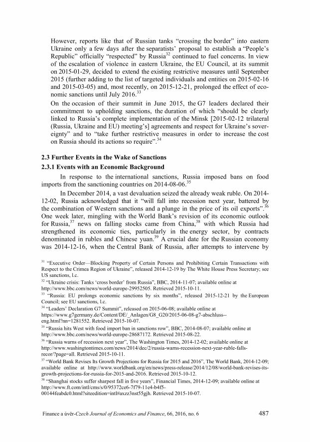
However, reports like that of Russian tanks “crossing the border” into eastern Ukraine only a few days after the separatists’ proposal to establish a “People’s Republic” officially “respected” by Russia32 continued to fuel concerns. In view of the escalation of violence in eastern Ukraine, the EU Council, at its summit on 2015-01-29, decided to extend the existing restrictive measures until September 2015 (further adding to the list of targeted individuals and entities on 2015-02-16 and 2015-03-05) and, most recently, on 2015-12-21, prolonged the effect of eco-nomic sanctions until July 2016.33 On the occasion of their summit in June 2015, the G7 leaders declared their commitment to upholding sanctions, the duration of which “should be clearly linked to Russia’s complete implementation of the Minsk [2015-02-12 trilateral (Russia, Ukraine and EU) meeting’s] agreements and respect for Ukraine’s sover-eignty” and to “take further restrictive measures in order to increase the cost on Russia should its actions so require”.34
2.3 Further Events in the Wake of Sanctions 2.3.1 Events with an Economic Background
In response to the international sanctions, Russia imposed bans on food imports from the sanctioning countries on 2014-08-06.35
In December 2014, a vast devaluation seized the already weak ruble. On 2014-12-02, Russia acknowledged that it “will fall into recession next year, battered by the combination of Western sanctions and a plunge in the price of its oil exports”.36 One week later, mingling with the World Bank’s revision of its economic outlook for Russia,37 news on falling stocks came from China,38 with which Russia had strengthened its economic ties, particularly in the energy sector, by contracts denominated in rubles and Chinese yuan.39 A crucial date for the Russian economy was 2014-12-16, when the Central Bank of Russia, after attempts to intervene by
31 “Executive Order—Blocking Property of Certain Persons and Prohibiting Certain Transactions with Respect to the Crimea Region of Ukraine”, released 2014-12-19 by The White House Press Secretary; seeUS sanctions, l.c. 32 “Ukraine crisis: Tanks ‘cross border’ from Russia”, BBC, 2014-11-07; available online at http://www.bbc.com/news/world-europe-29952505. Retrieved 2015-10-11. 33 “Russia: EU prolongs economic sanctions by six months”, released 2015-12-21 by the European Council; see EU sanctions, l.c. 34 “Leaders’ Declaration G7 Summit”, released on 2015-06-08; available online at https://www.g7germany.de/Content/DE/_Anlagen/G8_G20/2015-06-08-g7-abschluss--eng.html?nn=1281552. Retrieved 2015-10-07. 35 “Russia hits West with food import ban in sanctions row”, BBC, 2014-08-07; available online at http://www.bbc.com/news/world-europe-28687172. Retrieved 2015-08-22. 36 “Russia warns of recession next year”, The Washington Times, 2014-12-02; available online at http://www.washingtontimes.com/news/2014/dec/2/russia-warns-recession-next-year-ruble-falls-recor/?page=all. Retrieved 2015-10-11. 37 “World Bank Revises Its Growth Projections for Russia for 2015 and 2016”, The World Bank, 2014-12-09;available online at http://www.worldbank.org/en/news/press-release/2014/12/08/world-bank-revises-its-growth-projections-for-russia-for-2015-and-2016. Retrieved 2015-10-12. 38 “Shanghai stocks suffer sharpest fall in five years”, Financial Times, 2014-12-09; available online at http://www.ft.com/intl/cms/s/0/95372ce6-7f79-11e4-b4f5-00144feabdc0.html?siteedition=intl#axzz3nst55gjh. Retrieved 2015-10-07.
488 Finance a úvěr-Czech Journal of Economics and Finance, 66, 2016, no. 6
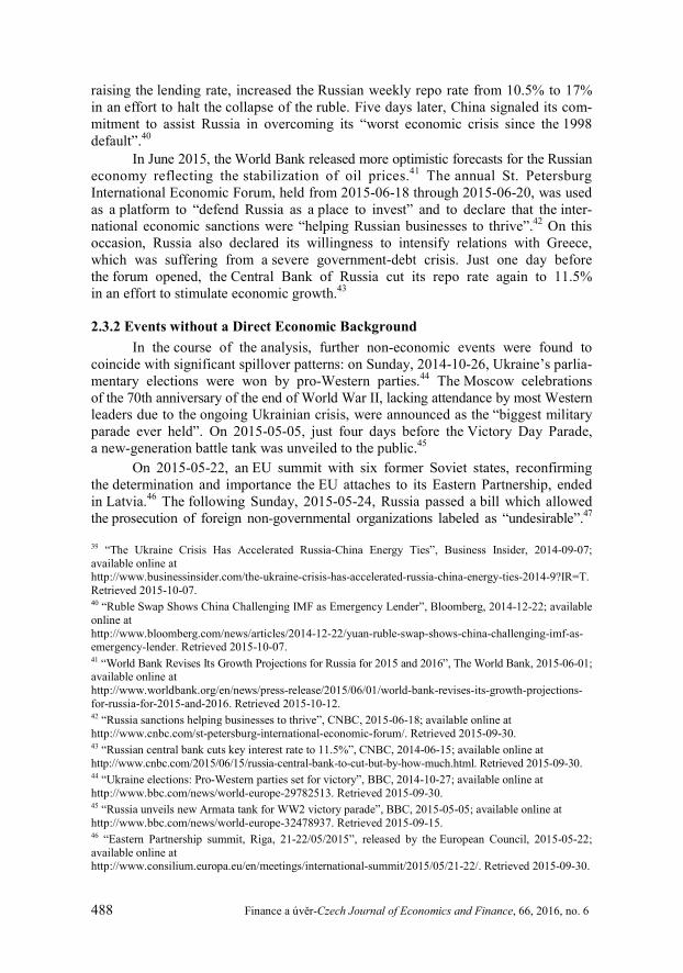
raising the lending rate, increased the Russian weekly repo rate from 10.5% to 17% in an effort to halt the collapse of the ruble. Five days later, China signaled its com-mitment to assist Russia in overcoming its “worst economic crisis since the 1998 default”.40
In June 2015, the World Bank released more optimistic forecasts for the Russian economy reflecting the stabilization of oil prices.41 The annual St. Petersburg International Economic Forum, held from 2015-06-18 through 2015-06-20, was used as a platform to “defend Russia as a place to invest” and to declare that the inter-national economic sanctions were “helping Russian businesses to thrive”.42 On this occasion, Russia also declared its willingness to intensify relations with Greece, which was suffering from a severe government-debt crisis. Just one day before the forum opened, the Central Bank of Russia cut its repo rate again to 11.5% in an effort to stimulate economic growth.43
2.3.2 Events without a Direct Economic Background In the course of the analysis, further non-economic events were found to
coincide with significant spillover patterns: on Sunday, 2014-10-26, Ukraine’s parlia-mentary elections were won by pro-Western parties.44 The Moscow celebrations of the 70th anniversary of the end of World War II, lacking attendance by most Western leaders due to the ongoing Ukrainian crisis, were announced as the “biggest military parade ever held”. On 2015-05-05, just four days before the Victory Day Parade, a new-generation battle tank was unveiled to the public.45
On 2015-05-22, an EU summit with six former Soviet states, reconfirming the determination and importance the EU attaches to its Eastern Partnership, ended in Latvia.46 The following Sunday, 2015-05-24, Russia passed a bill which allowed the prosecution of foreign non-governmental organizations labeled as “undesirable”.47
39 “The Ukraine Crisis Has Accelerated Russia-China Energy Ties”, Business Insider, 2014-09-07; available online at http://www.businessinsider.com/the-ukraine-crisis-has-accelerated-russia-china-energy-ties-2014-9?IR=T. Retrieved 2015-10-07. 40 “Ruble Swap Shows China Challenging IMF as Emergency Lender”, Bloomberg, 2014-12-22; available online at http://www.bloomberg.com/news/articles/2014-12-22/yuan-ruble-swap-shows-china-challenging-imf-as-emergency-lender. Retrieved 2015-10-07. 41 “World Bank Revises Its Growth Projections for Russia for 2015 and 2016”, The World Bank, 2015-06-01;available online at http://www.worldbank.org/en/news/press-release/2015/06/01/world-bank-revises-its-growth-projections-for-russia-for-2015-and-2016. Retrieved 2015-10-12. 42 “Russia sanctions helping businesses to thrive”, CNBC, 2015-06-18; available online at http://www.cnbc.com/st-petersburg-international-economic-forum/. Retrieved 2015-09-30. 43 “Russian central bank cuts key interest rate to 11.5%”, CNBC, 2014-06-15; available online at http://www.cnbc.com/2015/06/15/russia-central-bank-to-cut-but-by-how-much.html. Retrieved 2015-09-30. 44 “Ukraine elections: Pro-Western parties set for victory”, BBC, 2014-10-27; available online at http://www.bbc.com/news/world-europe-29782513. Retrieved 2015-09-30. 45 “Russia unveils new Armata tank for WW2 victory parade”, BBC, 2015-05-05; available online at http://www.bbc.com/news/world-europe-32478937. Retrieved 2015-09-15. 46 “Eastern Partnership summit, Riga, 21-22/05/2015”, released by the European Council, 2015-05-22; available online at http://www.consilium.europa.eu/en/meetings/international-summit/2015/05/21-22/. Retrieved 2015-09-30.
Finance a úvěr-Czech Journal of Economics and Finance, 66, 2016, no. 6 489
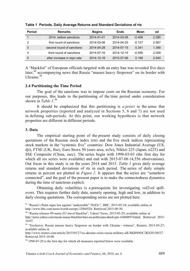
Table 1 Periods, Daily Average Returns and Standard Deviations of rts
Period Remarks Begins Ends Mean sd
1 2014, before sanctions 2014-01-01 2014-03-05 -0.406 2.285 2 first round of sanctions 2014-03-06 2014-04-25 -0.127 2.067 3 second round of sanctions 2014-04-28 2014-07-15 0.341 1.390 4 third round of sanctions 2014-07-16 2014-12-15 -0.558 2.009 5 after increase in repo rate 2014-12-16 2015-07-06 0.199 2.840
A “blacklist” of European officials targeted with an entry ban was revealed five days later,48 accompanying news that Russia “masses heavy firepower” on its border with Ukraine.49
2.4 Partitioning the Time Period The goal of the sanctions was to impose costs on the Russian economy. For
our purposes, this leads to the partitioning of the time period under consideration shown in Table 1.50
It should be emphasized that this partitioning is a priori in the sense that network properties (reported and analyzed in Sections 5, 6 and 7) are not used in defining sub-periods. At this point, our working hypothesis is that network properties are different in different periods.
3. Data The empirical starting point of the present study consists of daily closing
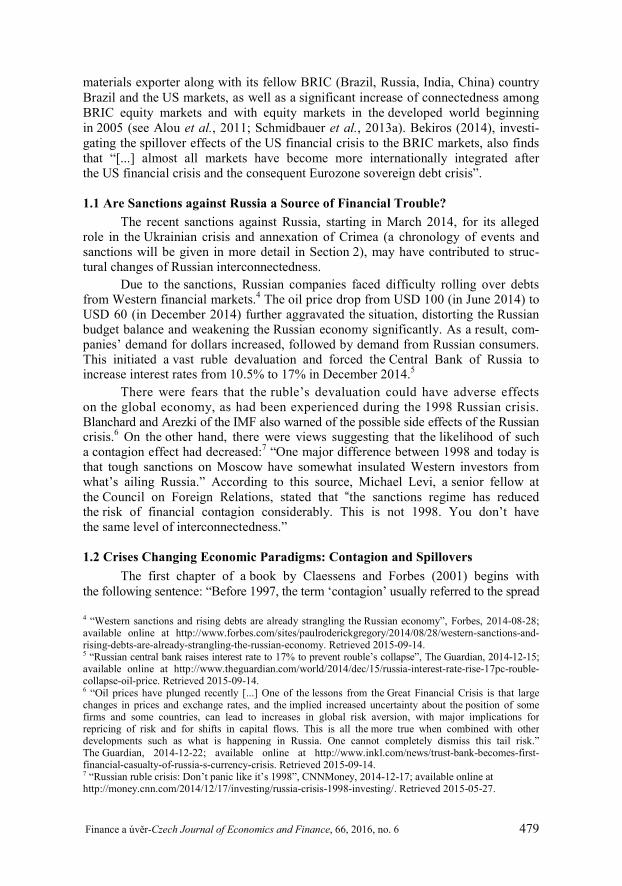
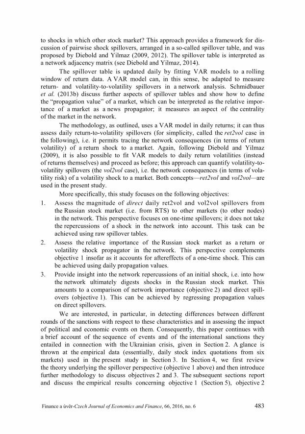
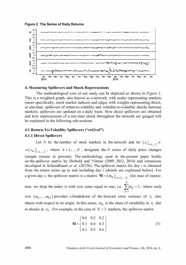
quotations of the Russian stock index (rts) and the five stock indices representing stock markets in the “systemic five” countries: Dow Jones Industrial Average (US, dji), FTSE (UK, ftse), Euro Stoxx 50 (euro area, sx5e), Nikkei 225 (Japan, n225) and SSE Composite (China, ssec). The series begin with 1998-03-03 (the first day for which all six series were available) and end with 2015-07-06 (4,556 observations). Our focus in this study is on the years 2014 and 2015. Table 1 gives daily average returns and standard deviations of rts in each period. The series of daily simple returns in percent are plotted in Figure 2. It appears that the series are “somehow connected”, and the goal of the present paper is to make the connectedness dynamics during the time of sanctions explicit.
Obtaining daily volatilities is a prerequisite for investigating vol2vol spill-overs. This requires further daily data, namely opening, high and low, in addition to daily closing quotations. The corresponding series are not plotted here. 47 “Russia’s Putin signs law against ‘undesirable” NGOs’”, BBC, 2015-05-24; available online at http://www.bbc.com/news/world-europe-32860526. Retrieved 2015-09-30. 48 “Russia releases 89-name EU travel blacklist”, Yahoo! News, 2015-05-29; available online at http://news.yahoo.com/russia-issues-blacklist-bars-eu-politicians-dutch-pm-164848974.html. Retrieved 2015-10-07. 49 “Exclusive: Russia masses heavy firepower on border with Ukraine—witness”, Reuters, 2015-05-27; available online at http://www.reuters.com/article/2015/05/27/us-ukraine-crisis-russia-military-idUSKBN0OC2K820150527. Retrieved 2015-10-08. 50 1998-07-20 is the first day for which all measures reported below were available.
490 Finance a úvěr-Czech Journal of Economics and Finance, 66, 2016, no. 6
Figure 2 The Series of Daily Returns
4. Measuring Spillovers and Shock Repercussions The methodological core of our study can be depicted as shown in Figure 1.
This is a weighted graph, also known as a network, with nodes representing markets (more specifically, stock market indices) and edges with weights representing direct, or one-time, spillovers of return-to-volatility and volatility-to-volatility shocks between markets; spillovers are updated on a daily basis. How direct spillovers are obtained and how repercussions of a one-time shock throughout the network are gauged will be explained in the following sub-sections.
4.1 Return-To-Volatility Spillovers (“ret2vol”) 4.1.1 Direct Spillovers
Let N be the number of stock markets in the network and let 1, ,t t Tx
1, , kt t Tx , where 1, , k N , designate the N series of daily price changes
(simple returns in percent). The methodology used in the present paper builds on the spillover matrix by Diebold and Yilmaz (2009, 2012, 2014) and extensions developed in Schmidbauer et al. (2013b). The spillover matrix for day t is obtained from the return series up to and including day t (details are explained below). For a given day t, the spillover matrix is a matrix , 1, , ik i k NmM (for ease of exposi-
tion, we drop the index t) with row sums equal to one, i.e. 1
1N
ikk
m , where each
row 1, , i iNm m provides a breakdown of the forecast error variance of ix into
shares with respect to its origin. In this sense, ikm is the share of variability in ix due to shocks in kx . For example, in the case of 3N markets, the spillover matrix
0.6 0.2 0.20.1 0.6 0.30.1 0.3 0.6
M (1)
Finance a úvěr-Czech Journal of Economics and Finance, 66, 2016, no. 6 491
means that 60% (20% each) of the forecast error variance of 1 x is due to shocks in 1 x itself (shocks in 2x and 3x , respectively). In other words: 40% of the volatility in market 1 is due to spillovers to market 1 from markets 2 and 3. Considering the first column of M, an “aggregate share” (column sums need not add up to 1) of 0.2 is spilled over from market 1 to markets 2 and 3, making market 1 a net receiver. Market 2 is a net giver.
Direct spillovers from market k (or to market i) are then given by the column (row, respectively) sums in M, excluding the market’s spillovers to itself:
1, 1,from market to others : ; to market from others :
N N
ik iki i k k k i
k m i m
Spillovers from market k to others, plus spillovers to itself, need not add up to 1. In social network terminology, with M interpreted as the adjacency matrix of a weighted directed network of nodes, these aggregates are the from-degree of node k (to-degree of node i, respectively); see Diebold and Yilmaz (2014).
For a given day t, the spillover matrix M is obtained as follows. The return series tx can be analyzed in terms of a structural VAR model in the form
0
t t ss
x s (2)
(where ( t ) is white noise with uncorrelated components) with impulse response
functions ,
ki i k
s s s , where ki s quantifies the response of itx to
a shock in ,k t s happening s time units earlier. Impulse response analysis is per-formed here in terms of an MA representation (2) with unit variance shocks. Thus,
quantifies the responses to shocks of size one standard deviation. The variance
of the n -period-ahead forecast of 1, ,ix i N can then be written as
1 2, ,
1 0var ˆ
N nk
i t n i t n ik s
x x s (3)
Equation (3) thus provides the link between return shocks and stock market volatility: it quantifies which amount of volatility in , i t nx originates from kt or,
equivalently, from a shock to return ktx . The forecast error variance decomposition (FEVD) is then expressed in terms of the ratios
1 2
01 2
1 0
, 1,...,
nki
sik N n
ki
k s
sm i N
s
Empirically, we fit a standard VAR model of order 1 to the N return series, using data from a window of size 100 (i.e. days t–99,…,t). We follow Diebold and Yilmaz (2014) and use an approach suggested by Pesaran and Shin (1998), namely:
492 Finance a úvěr-Czech Journal of Economics and Finance, 66, 2016, no. 6
in order to identify the impulse response function of a component (here, kx ), give the highest priority to that component; this removes the dependence on an imposed hierarchy of markets. Forecasting n steps ahead (we use n = 5), FEVD yields forecast error variance shares 1, ,i iNm m . With n = 5, the decomposition of forecast error variance is acceptably settled. This procedure is then applied for every t, resulting in a sequence of spillover matrices, which are the adjacency matrices for the network shown in Figure 1.
4.1.2 Relative Importance of a Market: Propagation Values The network structure of the spillover matrix with respect to the propagation
of shocks lends itself to a broader perspective, elaborated in Schmidbauer et al. (2013b). Let M again denote the spillover matrix for day t. We assume that M contains all relevant and the most recent available information about the network. A hypothetical shock (“news”, “information”) of unit size in market k on day t can be denoted as 0n (0,…,0,1,0,…,0)´, where 1 is in the k-th component of 0n . We assume that the propagation of this shock across the markets within day t will take place at short time intervals of unspecified length according to
1 , 0,1,2,s s sn Mn (4)
(where step 0s initializes the recursion). The index s in equation (4) therefore denotes a step in information flow. Moreover, assuming that information flow across markets can proceed instantly on day t, with spillover conditions (given by M) persisting throughout day t, it makes sense to investigate steady-state properties (as s ) of the model defined by equation (4). This leads to
v v M
When the left eigenvector ν = (ν1,…,νN)´ is normed so that 1
1, N
kk
v we call
kv the propagation value of market k. It renders the value of a return shock in market k as a seed for future uncertainty in returns across the network of markets:
1
N
k ik ii
v m v
For M, as in Equation (1), 0.2, 0.4, 0.4v , which means that a shock in market 2 is twice as powerful ( 0.4 / 0.2 2 ) as a shock in market 1 in terms of creating network volatility. A similar concept, eigenvector centrality, is also used in social network analysis; see, for example, Bonacich (1987).
4.1.3 Network Repercussions of a Shock Direct spillovers from market k to other markets measure the direct impact
of a shock in kx on day t without consideration of the immediate (i.e. also happening on day t) network repercussions of the shock. The propagation value of market k, in contrast, emphasizes the importance of shocks in kx within the network, including
Finance a úvěr-Czech Journal of Economics and Finance, 66, 2016, no. 6 493
repercussions throughout the network. Owing to different magnitudes, direct spill-overs from market k and the propagation values of market k cannot be directly compared. However, they can be related to each other via a regression
propagation valuet = α + β · spillovert + εt
where propagation valuet (spillovert) denotes the propagation value of market k (direct spillovers from market k, respectively) on day t. The residuals εt can be interpreted as propagation values (or the relative network importance) of market k, from which direct spillovers have been computationally removed. What remains is a measure of network repercussions of a direct spillover, i.e. the repercussions of a one-time shock in market k throughout the network, once again assuming that the spillover matrix is the only relevant information structure for a given day. There-fore, εt indicates the prevailing effect:
εt network repercussions are more important than direct spillovers on day
spillovers have only minor repercussionsin the netw0 :0 : direc ork on d y t a
tt
This methodology will be applied in Section 7, where market k designates the Russian stock market.
4.2 Volatility-To-Volatility Spillovers (“vol2vol”) The methodology outlined in Section 4.1 can also be applied to a set of series
1, , ˆkt t T , 1, ,k N , of daily volatilities, in lieu of returns (Diebold and Yilmaz,
2009). One difficulty to overcome is that daily volatilities cannot be directly observed and need to be reconstructed. Using daily GARCH variances is not the best way to represent volatilities, as a GARCH model forecasts variances but does not pick up what actually happened on a given day. Following Diebold and Yilmaz (2009), we use a method proposed by Garman and Klass (1980), based on the hypothesis that the stock price process is a geometric Brownian motion, to obtain daily variances. Their method results in the following formula:
22ˆ 0.511
0.019 2 2
0.383
kt kt kt
kt kt kt kt kt kt kt kt kt
kt kt
H L
C O H L O H O L O
C O
(5)
where ktO ( ktH , ktL , ktC ) designates the natural logarithm of the daily opening price (daily high, daily low, daily closing, respectively) of stock index k on day t. The series ˆkt constitute the input into VAR models along the lines explained in Section 4.1 to obtain daily direct spillovers, propagation values and network repercussions in the vol2vol case. In this case, direct spillovers characterize volatility- to-volatility spillovers, while the propagation values quantify the importance of a market with respect to the propagation of a volatility shock across markets, i.e. the value of a volatility shock from that market as a seed for future uncertainty in volatility across the network of markets. The term uncertainty in volatility results from con-sidering forecast error variances of volatilities.
494 Finance a úvěr-Czech Journal of Economics and Finance, 66, 2016, no. 6
The ADF test and the Phillips-Perron test reject the null hypothesis of non-stationarity for all volatility series used in our study. It is known that logarithmic volatility series are approximately normally distributed; see, for example, Andersen et al. (2001). However, logarithmic volatility goes to as volatility itself approaches 0. Volatility near 0 in a market on day t means that this market will hardly be a source of volatility spillovers, while this is what an absolutely large negative logarithmic volatility would imply. Small volatilities must not be (absolutely) amplified for our purposes. Furthermore, a VAR model needs Gaussian series if statistical inference concerning the parameters is intended. However, the purpose of the present paper is not to conduct statistical inference—the goal is to obtain the FEVD, which is basically a descriptive procedure.
The methodology outlined in this section will now be applied to the data described in Section 3. In view of our focus on the Ukrainian crisis, only results con-cerning 2014 and 2015 will be reported and discussed in the following three sections.
5. Direct Spillovers from and to rts This section reports the first part of spillover characteristics of the Russian
stock market, namely direct return and volatility spillovers, without considering potential aftereffects of a shock. Sections 6 and 7 will give more detailed inter-pretations using the methodological innovations (propagation values and network repercussions) introduced in Sections 4.1.2 and 4.1.3. Particular attention will be given to the following periods and events (cf. Section 2): End of period 1 / beginning of period 2 (roughly late January 2014–early
March 2014): Russia increased the economic pressure on Ukraine. The Olympic Games began in Sochi, Russia. In the run-up to the first round of sanctions, Russia’s president was granted parliamentary authorization to “use force in Ukraine to protect Russian interests”.
Beginning of period 4 (roughly the second half of July 2014): The third round of sanctions entailed extensive sectoral measures targeting Russia’s economy on a broad base, while the first and second rounds had imposed travel bans and asset freezes on Russian individuals and entities. The US was the first to take this step. The downing of the Malaysian airliner worsened the relations between Russia and Western countries to the effect that the EU joined, and tightened, economic sanctions two weeks later.
End of period 4 / beginning of period 5 (roughly late October 2014–December 2014): Ukraine’s parliamentary elections were won by pro-Western parties. Falling crude oil prices further aggravated Russia’s economic situation, leading Russia to acknowledge that it was heading towards a recession. A ruble crisis was triggered, which finally made the Central Bank of Russia increase the weekly repo rate significantly.
Later part of period 5 (roughly May–June 2015): Russia’s Victory Day Parade in early May was received in the Western world as a display of Russian military strength. Later that month, reports that Russia was massing military power on its border with Ukraine further strained relations between Russia and the EU. The St. Petersburg International Economic Forum held in mid-June was used as a platform to advertise businesses and investments in Russia.
Finance a úvěr-Czech Journal of Economics and Finance, 66, 2016, no. 6 495
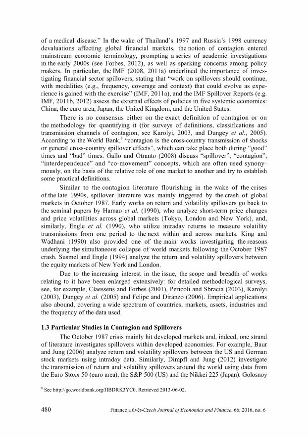
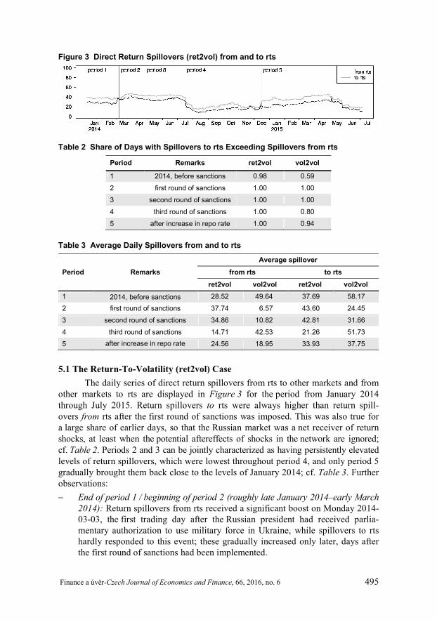
Figure 3 Direct Return Spillovers (ret2vol) from and to rts
Table 2 Share of Days with Spillovers to rts Exceeding Spillovers from rts
Period Remarks ret2vol vol2vol
1 2014, before sanctions 0.98 0.59 2 first round of sanctions 1.00 1.00 3 second round of sanctions 1.00 1.00 4 third round of sanctions 1.00 0.80 5 after increase in repo rate 1.00 0.94
Table 3 Average Daily Spillovers from and to rts
Period Remarks Average spillover
from rts to rts ret2vol vol2vol ret2vol vol2vol
1 2014, before sanctions 28.52 49.64 37.69 58.17 2 first round of sanctions 37.74 6.57 43.60 24.45 3 second round of sanctions 34.86 10.82 42.81 31.66 4 third round of sanctions 14.71 42.53 21.26 51.73 5 after increase in repo rate 24.56 18.95 33.93 37.75
5.1 The Return-To-Volatility (ret2vol) Case The daily series of direct return spillovers from rts to other markets and from
other markets to rts are displayed in Figure 3 for the period from January 2014 through July 2015. Return spillovers to rts were always higher than return spill- overs from rts after the first round of sanctions was imposed. This was also true for a large share of earlier days, so that the Russian market was a net receiver of return shocks, at least when the potential aftereffects of shocks in the network are ignored; cf. Table 2. Periods 2 and 3 can be jointly characterized as having persistently elevated levels of return spillovers, which were lowest throughout period 4, and only period 5 gradually brought them back close to the levels of January 2014; cf. Table 3. Further observations: End of period 1 / beginning of period 2 (roughly late January 2014–early March
2014): Return spillovers from rts received a significant boost on Monday 2014-03-03, the first trading day after the Russian president had received parlia-mentary authorization to use military force in Ukraine, while spillovers to rts hardly responded to this event; these gradually increased only later, days after the first round of sanctions had been implemented.
496 Finance a úvěr-Czech Journal of Economics and Finance, 66, 2016, no. 6
Beginning of period 4 (roughly the second half of July 2014): On 2014-07-18, one day after the downing of the Malaysian airliner, both return spillover series plunged towards levels which were below those held in January 2014. The imple-mentation of economic sanctions by the EU on 2014-07-31 coincided with further sliding.
End of period 4 / beginning of period 5 (roughly late October 2014–December 2014): The advent of the ruble crisis was accompanied by return spillovers moving closer to each other and, during the most dramatic days in mid-December, embarking on a zigzag course. From 2014-12-16 (the day of the repo rate increase) onwards, spillovers from rts started to stabilize, while spillovers to rts rose sharply the following day. An enlarged gap between return spillovers lasted for about four months, with both spillovers gradually increasing.
Later part of period 5 (roughly May–June 2015): The gap between return spill-overs narrowed again with a temporary significant boost in spillovers from rts when Russia unveiled its new battle tank in the run-up to its Victory Day Parade on 2015-05-09. From that time onwards, a simultaneous decrease in both series can be observed, with another visible plunge on 2014-05-27, the day when, amid political issues, Russia was reported to be massing military force on its border with Ukraine.
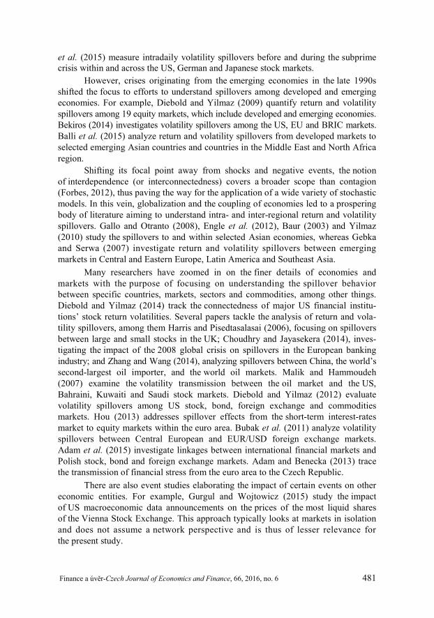
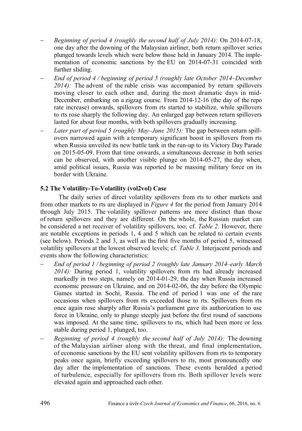
5.2 The Volatility-To-Volatility (vol2vol) Case The daily series of direct volatility spillovers from rts to other markets and
from other markets to rts are displayed in Figure 4 for the period from January 2014 through July 2015. The volatility spillover patterns are more distinct than those of return spillovers and they are different. On the whole, the Russian market can be considered a net receiver of volatility spillovers, too; cf. Table 2. However, there are notable exceptions in periods 1, 4 and 5 which can be related to certain events (see below). Periods 2 and 3, as well as the first five months of period 5, witnessed volatility spillovers at the lowest observed levels; cf. Table 3. Interjacent periods and events show the following characteristics: End of period 1 / beginning of period 2 (roughly late January 2014–early March
2014): During period 1, volatility spillovers from rts had already increased markedly in two steps, namely on 2014-01-29, the day when Russia increased economic pressure on Ukraine, and on 2014-02-06, the day before the Olympic Games started in Sochi, Russia. The end of period 1 was one of the rare occasions when spillovers from rts exceeded those to rts. Spillovers from rts once again rose sharply after Russia’s parliament gave its authorization to use force in Ukraine, only to plunge steeply just before the first round of sanctions was imposed. At the same time, spillovers to rts, which had been more or less stable during period 1, plunged, too.
Beginning of period 4 (roughly the second half of July 2014): The downing of the Malaysian airliner along with the threat, and final implementation, of economic sanctions by the EU sent volatility spillovers from rts to temporary peaks once again, briefly exceeding spillovers to rts, most pronouncedly one day after the implementation of sanctions. These events heralded a period of turbulence, especially for spillovers from rts. Both spillover levels were elevated again and approached each other.
Finance a úvěr-Czech Journal of Economics and Finance, 66, 2016, no. 6 497
Figure 4 Direct Volatility Spillovers (vol2vol) from and to rts
End of period 4 / beginning of period 5 (roughly late October 2014–December
2014): Turbulence in volatility spillovers increased towards the end of period 4, when the ruble crisis was becoming obvious. While spillovers to rts spiked with news of lower stock prices coming in from China on 2014-12-09, spill-overs from rts soared dramatically on 2014-12-16, the day of the repo rate increase, only to plunge the following day. From then onwards, volatility spillovers started to stabilize at low levels and with an enlarged gap between them for the following five months.
Later part of period 5 (roughly May–June 2015): Again, volatility spillovers switched into turbulence mode in early May, when Russia demonstrated its military determination on the occasion of its Victory Day Parade. Spillovers from rts were elevated throughout the month, temporarily exceeding spillovers to rts, amid further military threats from Russia and concerns of a renewal of the Cold War.
5.3 Discussion The behavior of both return spillovers (ret2vol) and volatility spillovers (vol2vol)
is clearly period-specific and there is strong evidence that political events impact stock market network characteristics.
The first and second rounds of sanctions do not differ with respect to either ret2vol or vol2vol patterns. The character of volatility spillovers, however, changed completely in the aftermath of the implementation of the third round of sanctions targeting banks and institutions. Volatility spillovers became more unpredictable, while return spillovers plunged to a low but more or less stable level. The increase of the repo rate appears to have had a stabilizing effect on volatility spillovers, pushing them back to lower levels. On the other hand, return spillovers increased.
Economic sanctions did not isolate Russia, but they did reduce ret2vol spill-overs from the Russian stock market. This reduction came at the cost of increased vol2vol spillovers and hence vulnerability, increasing the risk across the network.
6. Propagation Values: Relative Importance of the Russian Stock Market This section reports the second part of spillover characteristics of the Russian
stock market, namely its relative importance as a return (ret2vol) and volatility (vol2vol) shock propagator in the network of the “systemic five” plus rts, measured using the corresponding propagation values. The propagation values of rts will be compared and related to those of the “systemic five” in the discussion below.
498 Finance a úvěr-Czech Journal of Economics and Finance, 66, 2016, no. 6
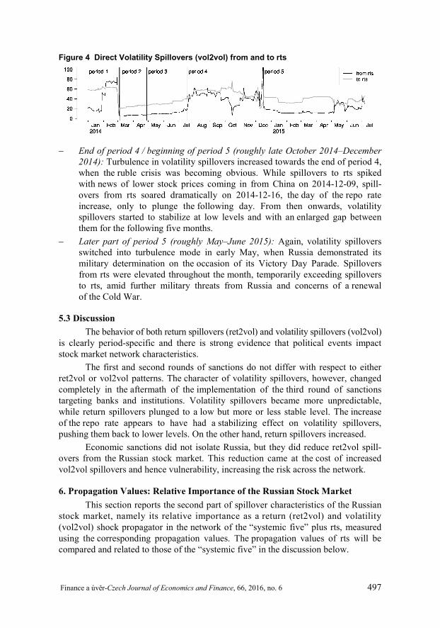
Figure 5 Propagation Values of rts, ret2vol
Table 4 Average Propagation Values, rts
Period Remarks ret2vol vol2vol
1 2014, before sanctions 0.143 0.148 2 first round of sanctions 0.180 0.055 3 second round of sanctions 0.177 0.064 4 third round of sanctions 0.135 0.146 5 after increase in repo rate 0.123 0.085
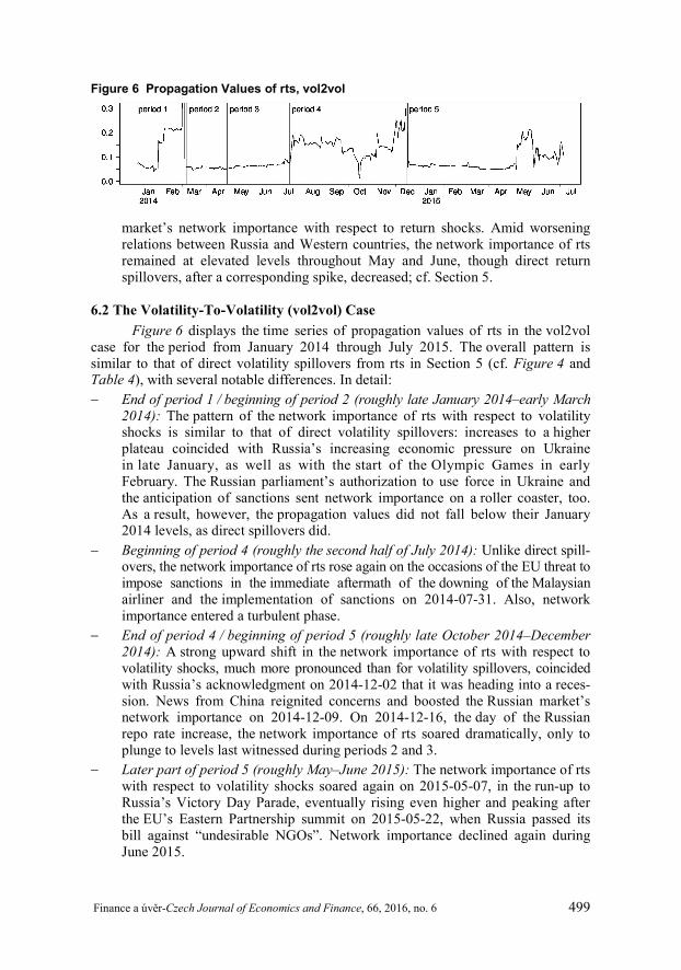
6.1 The Return-To-Volatility (ret2vol) Case Figure 5 displays the time series of propagation values of rts in the ret2vol
case for the period from January 2014 through July 2015. Persistently high levels of network importance of rts are observed during periods 2 and 3, while network importance was lowest during the first five months of period 5, unlike direct return spillovers from rts in Section 5; cf. Table 4 for averages. In particular: End of period 1 / beginning of period 2 (roughly late January 2014–early March
2014): On the first trading day after the Russian parliament approved the use of military force in Ukraine, the network importance of rts shifted abruptly upward. With the implementation of the first round of sanctions, it gradually abated to a still-high plateau where it remained more or less constant throughout periods 2 and 3.
Beginning of period 4 (roughly the second half of July 2014): The onset of eco-nomic sanctions imposed by the US was marked by a steady decrease in the net-work importance of rts, with a few flare-ups when the EU finally joined this round on 2014-07-31. On the other hand, the downing of the Malaysian airliner does not seem to leave any traces. The decrease in network importance con-tinued until mid-August. The network importance of rts hardly reached its January 2014 levels during period 4, though the September expansions of the sanc-tions and the ruble crisis are visible.
End of period 4 / beginning of period 5 (roughly late October 2014–December 2014): The dramatic days of the ruble crisis witnessed mild turbulence in the net-work importance of rts. The Russian repo rate increase, however, coincided with an abrupt and deep plunge in network importance to its lowest level since 2008, while direct spillovers increased; cf. Section 5. In the aftermath, the net-work importance of rts also started to increase, albeit slowly.
Later part of period 5 (roughly May–June 2015): The run-up to Russia’s Victory Day Parade on 2015-05-09 marked an abrupt upward shift in the Russian
Finance a úvěr-Czech Journal of Economics and Finance, 66, 2016, no. 6 499
Figure 6 Propagation Values of rts, vol2vol
market’s network importance with respect to return shocks. Amid worsening relations between Russia and Western countries, the network importance of rts remained at elevated levels throughout May and June, though direct return spillovers, after a corresponding spike, decreased; cf. Section 5.
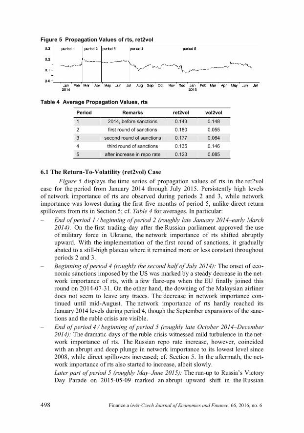
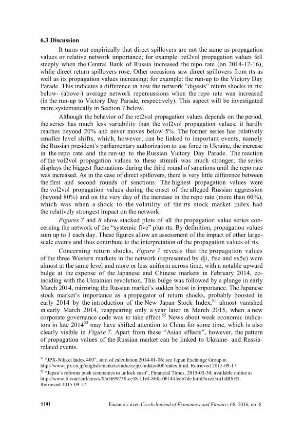
6.2 The Volatility-To-Volatility (vol2vol) Case Figure 6 displays the time series of propagation values of rts in the vol2vol
case for the period from January 2014 through July 2015. The overall pattern is similar to that of direct volatility spillovers from rts in Section 5 (cf. Figure 4 and Table 4), with several notable differences. In detail: End of period 1 / beginning of period 2 (roughly late January 2014–early March
2014): The pattern of the network importance of rts with respect to volatility shocks is similar to that of direct volatility spillovers: increases to a higher plateau coincided with Russia’s increasing economic pressure on Ukraine in late January, as well as with the start of the Olympic Games in early February. The Russian parliament’s authorization to use force in Ukraine and the anticipation of sanctions sent network importance on a roller coaster, too. As a result, however, the propagation values did not fall below their January 2014 levels, as direct spillovers did.
Beginning of period 4 (roughly the second half of July 2014): Unlike direct spill-overs, the network importance of rts rose again on the occasions of the EU threat to impose sanctions in the immediate aftermath of the downing of the Malaysian airliner and the implementation of sanctions on 2014-07-31. Also, network importance entered a turbulent phase.
End of period 4 / beginning of period 5 (roughly late October 2014–December 2014): A strong upward shift in the network importance of rts with respect to volatility shocks, much more pronounced than for volatility spillovers, coincided with Russia’s acknowledgment on 2014-12-02 that it was heading into a reces-sion. News from China reignited concerns and boosted the Russian market’s network importance on 2014-12-09. On 2014-12-16, the day of the Russian repo rate increase, the network importance of rts soared dramatically, only to plunge to levels last witnessed during periods 2 and 3.
Later part of period 5 (roughly May–June 2015): The network importance of rts with respect to volatility shocks soared again on 2015-05-07, in the run-up to Russia’s Victory Day Parade, eventually rising even higher and peaking after the EU’s Eastern Partnership summit on 2015-05-22, when Russia passed its bill against “undesirable NGOs”. Network importance declined again during June 2015.
500 Finance a úvěr-Czech Journal of Economics and Finance, 66, 2016, no. 6
6.3 Discussion It turns out empirically that direct spillovers are not the same as propagation
values or relative network importance; for example: ret2vol propagation values fell steeply when the Central Bank of Russia increased the repo rate (on 2014-12-16), while direct return spillovers rose. Other occasions saw direct spillovers from rts as well as its propagation values increasing; for example: the run-up to the Victory Day Parade. This indicates a difference in how the network “digests” return shocks in rts: below- (above-) average network repercussions when the repo rate was increased (in the run-up to Victory Day Parade, respectively). This aspect will be investigated more systematically in Section 7 below.
Although the behavior of the ret2vol propagation values depends on the period, the series has much less variability than the vol2vol propagation values; it hardly reaches beyond 20% and never moves below 5%. The former series has relatively smaller level shifts, which, however, can be linked to important events, namely the Russian president’s parliamentary authorization to use force in Ukraine, the increase in the repo rate and the run-up to the Russian Victory Day Parade. The reaction of the vol2vol propagation values to these stimuli was much stronger; the series displays the biggest fluctuations during the third round of sanctions until the repo rate was increased. As in the case of direct spillovers, there is very little difference between the first and second rounds of sanctions. The highest propagation values were the vol2vol propagation values during the onset of the alleged Russian aggression (beyond 80%) and on the very day of the increase in the repo rate (more than 60%), which was when a shock to the volatility of the rts stock market index had the relatively strongest impact on the network.
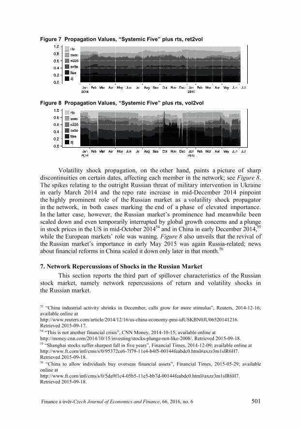
Figures 7 and 8 show stacked plots of all the propagation value series con-cerning the network of the “systemic five” plus rts. By definition, propagation values sum up to 1 each day. These figures allow an assessment of the impact of other large-scale events and thus contribute to the interpretation of the propagation values of rts.
Concerning return shocks, Figure 7 reveals that the propagation values of the three Western markets in the network (represented by dji, ftse and sx5e) were almost at the same level and more or less uniform across time, with a notable upward bulge at the expense of the Japanese and Chinese markets in February 2014, co-inciding with the Ukrainian revolution. This bulge was followed by a plunge in early March 2014, mirroring the Russian market’s sudden boost in importance. The Japanese stock market’s importance as a propagator of return shocks, probably boosted in early 2014 by the introduction of the New Japan Stock Index,51 almost vanished in early March 2014, reappearing only a year later in March 2015, when a new corporate governance code was to take effect.52 News about weak economic indica-tors in late 201453 may have shifted attention to China for some time, which is also clearly visible in Figure 7. Apart from these “Asian effects”, however, the pattern of propagation values of the Russian market can be linked to Ukraine- and Russia-related events. 51 “JPX-Nikkei Index 400”, start of calculation 2014-01-06; see Japan Exchange Group at http://www.jpx.co.jp/english/markets/indices/jpx-nikkei400/index.html. Retrieved 2015-09-17. 52 “Japan’s reforms push companies to unlock cash”, Financial Times, 2015-03-30; available online at http://www.ft.com/intl/cms/s/0/a5699738-ce58-11e4-86fc-00144feab7de.html#axzz3m1slR6H7. Retrieved 2015-09-17.
Finance a úvěr-Czech Journal of Economics and Finance, 66, 2016, no. 6 501
Figure 7 Propagation Values, “Systemic Five” plus rts, ret2vol
Figure 8 Propagation Values, “Systemic Five” plus rts, vol2vol
Volatility shock propagation, on the other hand, paints a picture of sharp discontinuities on certain dates, affecting each member in the network; see Figure 8. The spikes relating to the outright Russian threat of military intervention in Ukraine in early March 2014 and the repo rate increase in mid-December 2014 pinpoint the highly prominent role of the Russian market as a volatility shock propagator in the network, in both cases marking the end of a phase of elevated importance. In the latter case, however, the Russian market’s prominence had meanwhile been scaled down and even temporarily interrupted by global growth concerns and a plunge in stock prices in the US in mid-October 201454 and in China in early December 2014,55 while the European markets’ role was waning. Figure 8 also unveils that the revival of the Russian market’s importance in early May 2015 was again Russia-related; news about financial reforms in China scaled it down only later in that month.56
7. Network Repercussions of Shocks in the Russian Market This section reports the third part of spillover characteristics of the Russian
stock market, namely network repercussions of return and volatility shocks in the Russian market.
53 “China industrial activity shrinks in December, calls grow for more stimulus”, Reuters, 2014-12-16; available online at http://www.reuters.com/article/2014/12/16/us-china-economy-pmi-idUSKBN0JU06520141216. Retrieved 2015-09-17. 54 “This is not another financial crisis”, CNN Money, 2014-10-15; available online at http://money.cnn.com/2014/10/15/investing/stocks-plunge-not-like-2008/. Retrieved 2015-09-18. 55 “Shanghai stocks suffer sharpest fall in five years”, Financial Times, 2014-12-09; available online at http://www.ft.com/intl/cms/s/0/95372ce6-7f79-11e4-b4f5-00144feabdc0.html#axzz3m1slR6H7. Retrieved 2015-09-18. 56 “China to allow individuals buy overseas financial assets”, Financial Times, 2015-05-29; available online at http://www.ft.com/intl/cms/s/0/5da9f1c4-05b5-11e5-bb7d-00144feabdc0.html#axzz3m1slR6H7. Retrieved 2015-09-18.
502 Finance a úvěr-Czech Journal of Economics and Finance, 66, 2016, no. 6
Figure 9 Network Repercussions of an rts Return Shock (ret2vol)
Figure 10 Network Repercussions of an rts Volatility Shock (vol2vol)
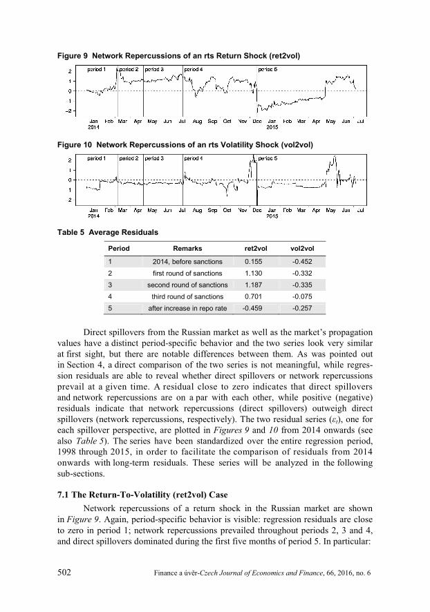
Table 5 Average Residuals
Period Remarks ret2vol vol2vol
1 2014, before sanctions 0.155 -0.452 2 first round of sanctions 1.130 -0.332 3 second round of sanctions 1.187 -0.335 4 third round of sanctions 0.701 -0.075 5 after increase in repo rate -0.459 -0.257
Direct spillovers from the Russian market as well as the market’s propagation
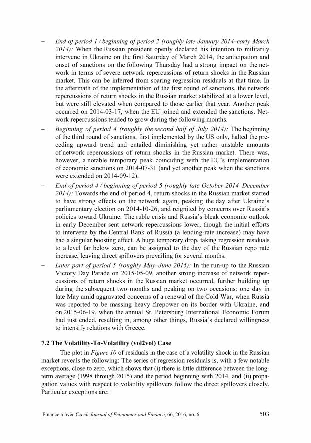
values have a distinct period-specific behavior and the two series look very similar at first sight, but there are notable differences between them. As was pointed out in Section 4, a direct comparison of the two series is not meaningful, while regres-sion residuals are able to reveal whether direct spillovers or network repercussions prevail at a given time. A residual close to zero indicates that direct spillovers and network repercussions are on a par with each other, while positive (negative) residuals indicate that network repercussions (direct spillovers) outweigh direct spillovers (network repercussions, respectively). The two residual series (εt), one for each spillover perspective, are plotted in Figures 9 and 10 from 2014 onwards (see also Table 5). The series have been standardized over the entire regression period, 1998 through 2015, in order to facilitate the comparison of residuals from 2014 onwards with long-term residuals. These series will be analyzed in the following sub-sections.
7.1 The Return-To-Volatility (ret2vol) Case Network repercussions of a return shock in the Russian market are shown
in Figure 9. Again, period-specific behavior is visible: regression residuals are close to zero in period 1; network repercussions prevailed throughout periods 2, 3 and 4, and direct spillovers dominated during the first five months of period 5. In particular:
Finance a úvěr-Czech Journal of Economics and Finance, 66, 2016, no. 6 503
End of period 1 / beginning of period 2 (roughly late January 2014–early March 2014): When the Russian president openly declared his intention to militarily intervene in Ukraine on the first Saturday of March 2014, the anticipation and onset of sanctions on the following Thursday had a strong impact on the net-work in terms of severe network repercussions of return shocks in the Russian market. This can be inferred from soaring regression residuals at that time. In the aftermath of the implementation of the first round of sanctions, the network repercussions of return shocks in the Russian market stabilized at a lower level, but were still elevated when compared to those earlier that year. Another peak occurred on 2014-03-17, when the EU joined and extended the sanctions. Net-work repercussions tended to grow during the following months.
Beginning of period 4 (roughly the second half of July 2014): The beginning of the third round of sanctions, first implemented by the US only, halted the pre-ceding upward trend and entailed diminishing yet rather unstable amounts of network repercussions of return shocks in the Russian market. There was, however, a notable temporary peak coinciding with the EU’s implementation of economic sanctions on 2014-07-31 (and yet another peak when the sanctions were extended on 2014-09-12).
End of period 4 / beginning of period 5 (roughly late October 2014–December 2014): Towards the end of period 4, return shocks in the Russian market started to have strong effects on the network again, peaking the day after Ukraine’s parliamentary election on 2014-10-26, and reignited by concerns over Russia’s policies toward Ukraine. The ruble crisis and Russia’s bleak economic outlook in early December sent network repercussions lower, though the initial efforts to intervene by the Central Bank of Russia (a lending-rate increase) may have had a singular boosting effect. A huge temporary drop, taking regression residuals to a level far below zero, can be assigned to the day of the Russian repo rate increase, leaving direct spillovers prevailing for several months.
Later part of period 5 (roughly May–June 2015): In the run-up to the Russian Victory Day Parade on 2015-05-09, another strong increase of network reper-cussions of return shocks in the Russian market occurred, further building up during the subsequent two months and peaking on two occasions: one day in late May amid aggravated concerns of a renewal of the Cold War, when Russia was reported to be massing heavy firepower on its border with Ukraine, and on 2015-06-19, when the annual St. Petersburg International Economic Forum had just ended, resulting in, among other things, Russia’s declared willingness to intensify relations with Greece.
7.2 The Volatility-To-Volatility (vol2vol) Case The plot in Figure 10 of residuals in the case of a volatility shock in the Russian
market reveals the following: The series of regression residuals is, with a few notable exceptions, close to zero, which shows that (i) there is little difference between the long-term average (1998 through 2015) and the period beginning with 2014, and (ii) propa-gation values with respect to volatility spillovers follow the direct spillovers closely. Particular exceptions are:
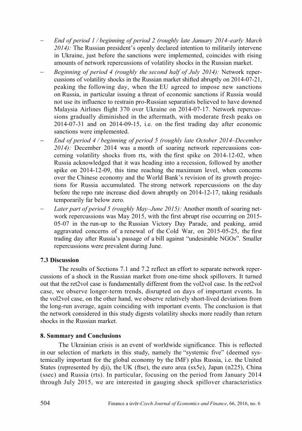
504 Finance a úvěr-Czech Journal of Economics and Finance, 66, 2016, no. 6
End of period 1 / beginning of period 2 (roughly late January 2014–early March 2014): The Russian president’s openly declared intention to militarily intervene in Ukraine, just before the sanctions were implemented, coincides with rising amounts of network repercussions of volatility shocks in the Russian market.
Beginning of period 4 (roughly the second half of July 2014): Network reper-cussions of volatility shocks in the Russian market shifted abruptly on 2014-07-21, peaking the following day, when the EU agreed to impose new sanctions on Russia, in particular issuing a threat of economic sanctions if Russia would not use its influence to restrain pro-Russian separatists believed to have downed Malaysia Airlines flight 370 over Ukraine on 2014-07-17. Network repercus-sions gradually diminished in the aftermath, with moderate fresh peaks on 2014-07-31 and on 2014-09-15, i.e. on the first trading day after economic sanctions were implemented.
End of period 4 / beginning of period 5 (roughly late October 2014–December 2014): December 2014 was a month of soaring network repercussions con-cerning volatility shocks from rts, with the first spike on 2014-12-02, when Russia acknowledged that it was heading into a recession, followed by another spike on 2014-12-09, this time reaching the maximum level, when concerns over the Chinese economy and the World Bank’s revision of its growth projec-tions for Russia accumulated. The strong network repercussions on the day before the repo rate increase died down abruptly on 2014-12-17, taking residuals temporarily far below zero.
Later part of period 5 (roughly May–June 2015): Another month of soaring net-work repercussions was May 2015, with the first abrupt rise occurring on 2015-05-07 in the run-up to the Russian Victory Day Parade, and peaking, amid aggravated concerns of a renewal of the Cold War, on 2015-05-25, the first trading day after Russia’s passage of a bill against “undesirable NGOs”. Smaller repercussions were prevalent during June.
7.3 Discussion The results of Sections 7.1 and 7.2 reflect an effort to separate network reper-
cussions of a shock in the Russian market from one-time shock spillovers. It turned out that the ret2vol case is fundamentally different from the vol2vol case. In the ret2vol case, we observe longer-term trends, disrupted on days of important events. In the vol2vol case, on the other hand, we observe relatively short-lived deviations from the long-run average, again coinciding with important events. The conclusion is that the network considered in this study digests volatility shocks more readily than return shocks in the Russian market.
8. Summary and Conclusions The Ukrainian crisis is an event of worldwide significance. This is reflected
in our selection of markets in this study, namely the “systemic five” (deemed sys-temically important for the global economy by the IMF) plus Russia, i.e. the United States (represented by dji), the UK (ftse), the euro area (sx5e), Japan (n225), China (ssec) and Russia (rts). In particular, focusing on the period from January 2014 through July 2015, we are interested in gauging shock spillover characteristics
Finance a úvěr-Czech Journal of Economics and Finance, 66, 2016, no. 6 505
of the Russian market in light of the events and international sanctions connected with the Ukrainian crisis, with a focus on detecting differences between different rounds of sanctions.
The methodology of this paper uses and extends the methodology developed by Diebold and Yilmaz (2009, 2012, 2014). It permits daily screening of network dynamics in terms of direct return-to-volatility (and volatility-to-volatility) spillovers from and to rts as well as in terms of repercussions of return (and volatility) shocks coming from rts. The latter is measured by a concept called the propagation value in the present paper; it measures the relative importance of a shock in a market as a seed for future uncertainty in returns (and volatilities) across the network. Together with direct spillovers, this also allows an assessment of whether direct spillovers or network repercussions of shocks are more important on a given day.
There is strong evidence that political and economic events, along with the international sanctions imposed so far in connection with the Ukrainian crisis, influenced the shock spillover characteristics of the Russian stock market.
On the one hand, we found period-specific behavior of direct spillovers and propagation values with respect to rounds of sanctions, concerning both return and volatility shocks in rts. While rounds 1 and 2 of the sanctions hardly differ with respect to their patterns, these change completely with the implementation of eco-nomic sanctions in round 3 and again after the Central Bank of Russia increased the weekly repo rate. When round 3 of sanctions commenced, direct spillovers as well as propagation values from return shocks in rts slumped back to the low levels held before the sanctions began (or to even lower levels), while those from volatility shocks entered a period of turbulence at elevated levels. This period ends abruptly with the day when the Central Bank of Russia increased the repo rate. In the after-math, the impact of volatility shocks in rts on the network was reduced considerably, while return shocks again became more important, though only with respect to direct spillovers: the propagation value of return (and volatility) shocks in rts initially plunged to its lowest level.
On the other hand, there are five prominent events, among them the repo rate increase, that coincided with a sudden explosion or downturn in network reper-cussions. Russia’s propagation values fell steeply when the Central Bank of Russia increased the repo rate, leaving network repercussions far below average. Two other events of direct economic relevance and having a strong impact on volatility shocks and network repercussions were the threat of economic sanctions by the EU after the downing of the Malaysian airliner in July 2014 and Russia’s acknowledgment that it was heading into a recession in early December 2014. The remaining two events, of a more political character, lead to explosions in network repercussions which were particularly pronounced for return shocks: the Russian president’s parlia-mentary pledge and authorization to use force in Ukraine in early March 2014 and Russia’s activities around the Victory Day Parade in May 2015; no other Victory Day since 1998 had such a big impact. This indicates a difference in how the network “digests” news.
In 2014, Russia’s GDP went down by 11.26% compared to 201357 and its trading volume with the EU had decreased to approximately EUR 300 billion.58 An analysis of the costs of the trade restrictions between the EU-27 plus Switzerland versus
506 Finance a úvěr-Czech Journal of Economics and Finance, 66, 2016, no. 6
Russia was conducted in a recent study by Christen et al. (2015). According to their estimate, the economies of the EU-27 plus Switzerland incurred short-run costs of EUR 34 billion in value added; similarly, the long-run costs are estimated to amount to EUR 92 billion.
The economic sanctions did not isolate Russia, but they did change its role as a shock propagator in the network of stock markets; they reduced the Russian stock market’s relative importance as a propagator of return shocks. We have shown that this reduction came at the cost of increasing the importance of the Russian stock market as a propagator of volatility shocks, thereby increasing the risk induced by volatility shocks across the network. The deterioration of the Russian economy, along with the ruble’s depreciation, could be responsible for this phenomenon; indeed, fears of a contagion effect similar to that seen in the 1990s were greater than before. With this observation in mind, it can be concluded that sanctions can be used as a policy tool to impose costs on the sanctioned economy. Sanctions are able to magnify an economy’s problems. But this can probably only be achieved at the expense of introducing more volatility into the entire network of stock markets and, in particular, making the network more vulnerable with respect to volatility shocks from the targeted stock market, with the effect that the sanctioning economies are faced with the backlash of their own sanctions.
The methodology adopted in our study lends itself also to an analysis of the con-sequences of the sanctions in connection with the Ukrainian crisis on networks consisting of local partners of Russia. This could be helpful in evaluating policy alternatives for economic entities considering imposing sanctions.
57 The authors’ own calculations, based on data provided by the World Bank; see http://data.worldbank.org/data-catalog/GDP-ranking-table. Retrieved 2015-05-21. 58 “European Union, Trade in goods with Russia”, released by the European Commission; available online athttp://trade.ec.europa.eu/doclib/docs/2006/september/tradoc_113440.pdf. Retrieved 2015-10-04.
Finance a úvěr-Czech Journal of Economics and Finance, 66, 2016, no. 6 507
REFERENCES
Adam M, Banbula P, Markun M (2015): International Dependence and Contagion across Asset Classes: The Case of Poland. Finance a úvěr-Czech Journal of Economics and Finance, 65(3): 254–270. Adam T, Benecka S (2013): Financial Stress Spillover and Financial Linkages between the Euro Area and the Czech Republic. Finance a úvěr-Czech Journal of Economics and Finance, 63(1): 46–64. Aloui R, Aissa MSB, Nguyen DK (2011): Global financial crisis, extreme interdependences, and contagion effects: The role of economic structure? Journal of Banking and Finance, 35(1):130–141. Andersen TG, Bollerslev T, Diebold FX, Ebens H (2001): The distribution of realized stock return volatility. Journal of Financial Economics, 61:43–76. Balli F, Hajhoj HR, Basher SA, Ghassan HB (2015): An analysis of returns and volatility spillovers and their determinants in emerging Asian and Middle Eastern countries. International Review of Economics and Finance, 39:311–325. Baur D (2003): Testing for contagion—Mean and volatility contagion. Journal of Multinational Financial Management, 13(4-5):405–422. Baur D, Jung RC (2006): Return and volatility linkages between the US and the German stock market. Journal of International Money and Finance, 25(4):598–613. Bekiros SD (2014): Contagion, decoupling and the spillover effects of the US financial crisis: Evidence from the BRIC markets. International Review of Financial Analysis, 33:58–69. Bonacich P (1987): Power and Centrality: A Family of Measures. American Journal of Sociology, 92(5):1170–1182. Bubak V, Kocenda E, Zikes F (2011): Volatility transmission in emerging European foreign exchange markets. Journal of Banking and Finance, 35(11):2829–2841. Choudhry T, Jayasekera R (2014): Returns and volatility spillover in the European banking industry during global financial crisis: Flight to perceived quality or contagion? International Review of Financial Analysis, 36:36–45. Christen E, Fritz O, Streicher G (2015): Effects of the EU-Russia Economic Sanctions on Value Added and Employment in the European Union and Switzerland. Austrian Institute of Economic Research, June 2015, 24 pages. Claessens S, Forbes K (2001): International Financial Contagion: An Overview of the Issues and the Book. In: Claessens S, Forbes K (Eds): International Financial Contagion. Springer Science + Business Media, New York, pp. 3–17. Demiralay S, Bayraci S (2015): Central and Eastern European Stock Exchanges under Stress: A Range-Based Volatility Spillover Framework. Finance a úvěr-Czech Journal of Economics and Finance, 65(5):411–430. Diebold FX, Yilmaz K (2009): Measuring Financial Asset Return and Volatility Spillovers, with Application to Global Equity Markets. Economic Journal, 119:158–171. Diebold FX, Yilmaz K (2012): Better to give than to receive: Predictive directional measurement of volatility spillovers. International Journal of Forecasting, 28(1):57–66. Diebold FX, Yilmaz K (2014): On the Network Topology of Variance Decompositions: Measuring the Connectedness of Financial Firms. Journal of Econometrics, 182(1):119–134. Dimpfl T, Jung RC (2012): Financial market spillovers around the globe. Applied Financial Economics, 22(1):45–57. Dungey M, Fry R, Gonzalez-Hermosillo B, Martin VL (2005): Empirical Modelling of Contagion: a Review of Methodologies. Quantitative Finance, 5(1):9–24. Engle RF, Gallo GM, Velucchi M (2012): Volatility Spillovers in East Asian Financial Markets: A MEM-Based Approach. The Review of Economics and Statistics, 94(1):222–233.
508 Finance a úvěr-Czech Journal of Economics and Finance, 66, 2016, no. 6
Engle RF, Ito T, Lin W-L (1990): Meteor showers or heat waves? Heteroskedastic intra-daily volatility in the foreign exchange market. Econometrica, 58(3):525–542. Fedorova E, Saleem K (2010): Volatility Spillovers between Stock and Currency Markets: Evidence from Emerging Eastern Europe. Finance a úvěr-Czech Journal of Economics and Finance, 60(6): 519–533. Felipe PS, Diranzo FC (2006): Volatility transmission models: a survey. Revista de Economia Financiera, 10(3):32–81. Forbes KJ (2012): The “Big C”: Identifying and Mitigating Contagion. Paper prepared for the 2012 Jackson Hole Symposium hosted by the Federal Reserve Bank of Kansas City on 08/31/12 to 09/01/12. Available at http://www.kansascityfed.org/publicat/sympos/2012/kf.pdf. Gallo GM, Otranto E (2008): Volatility spillovers, interdependence and comovements: A Markov Switching approach. Computational Statistics and Data Analysis, 52(6):3011–3026. Garman MB, Klass MJ (1980): On the Estimation of Security Price Volatilities from Historical Data. The Journal of Business, 53(1):67–78. Gebka B, Serwa D (2007): Intra- and inter-regional spillovers between emerging capital markets around the world. Research in International Business and Finance, 21(2):203–221. Golosnoy V, Gribisch B, Liesenfeld R (2015): Intra-daily volatility spillovers in international stock markets. Journal of International Money and Finance, 53:95–114. Gurgul H, Wojtowicz T (2015): The Response of Intraday ATX Returns to U.S. Macroeconomic News. Finance a úvěr-Czech Journal of Economics and Finance, 65(3):230–253. Hamao Y, Masulis RW, Ng V (1990): Correlations in Price Changes and Volatility across International Stock Markets. The Review of Financial Studies, 3(2):281–307. Harris RDF, Pisedtasalasai A (2006): Return and Volatility Spillovers between Large and Small Stocks in the UK. Journal of Business Finance and Accounting, 33(9-10):1556–1571. Hou AJ (2013): EMU equity markets’ return variance and spillover effects from the short-term interest rate. Quantitative Finance, 13(3):451–470. IMF (2008): 2008 Triennial Surveillance Review—Overview Paper. International Monetary Fund, Washington D.C. IMF (2011a): 2011 Triennial Surveillance Review—Overview Paper. International Monetary Fund, Washington D.C. IMF (2011b): 2011 Consolidated Spillover Report: Implications from the Analysis of the Systemic-5. International Monetary Fund, Washington D.C. IMF (2012): 2012 Spillover Report—Background Papers. International Monetary Fund, Washington D.C. Karolyi GA (2003): Does International Financial Contagion Really Exist? International Finance, 6(2):179–199. King MA, Wadhwani S (1990): Transmission of Volatility between Stock Markets. The Review of Financial Studies, 3(1):5–33. Lee Y-H, Fang H, Su W-F (2014): Effectiveness of Portfolio Diversification and the Dynamic Relationship between Stock and Currency Markets in the Emerging Eastern European and Russian Markets. Finance a úvěr-Czech Journal of Economics and Finance, 64(4):296–311. Malik F, Hammoudeh S (2007): Shock and volatility transmission in the oil, US and Gulf equity markets. International Review of Economics and Finance, 16(3):357–368. Pericoli M, Sbracia M (2003): A Primer on Financial Contagion. Journal of Economic Surveys, 17(4):571–608. Pesaran HH, Shin Y (1998): Generalized impulse response analysis in linear multivariate models. Economics Letters, 58(1):17–29. R Core Team (2015): R: A Language and Environment for Statistical Computing. R Foundation for Statistical Computing, Vienna, Austria.
Finance a úvěr-Czech Journal of Economics and Finance, 66, 2016, no. 6 509
Schmidbauer H, Rösch A, Uluceviz E (2013a): Information Propagation between Equity Markets: the Case of BRICT. In: EcoMod Network (Ed.): Proceedings of the International Conference on Policy Modeling EcoMod 2013. Prague, July 1–3, 2013. Schmidbauer H, Rösch A, Uluceviz E (2013b): Market Connectedness: Spillovers, Information Flow, and Relative Market Entropy. Koç University–TÜSİAD Economic Research Forum, Working Paper, no. 1320 (October 2013). Available at http://eaf.ku.edu.tr/sites/eaf.ku.edu.tr/files/erf_wp_1320.pdf. Susmel R, Engle RF (1994): Hourly volatility spillovers between international equity markets. Journal of International Money and Finance, 13(1):3–25. Yilmaz K (2010): Return and volatility spillovers among the East Asian equity markets. Journal of Asian Economics, 21(3):304–313. Zhang B, Wang P (2014): Return and volatility spillovers between China and world oil markets. Economic Modelling, 42:413–420. Zivkov D, Njegic J, Milenkovic I (2015): Bidirectional Volatility Spillover Effect between the Exchange Rate and Stocks in the Presence of Structural Breaks in Selected Eastern European Economies. Finance a úvěr-Czech Journal of Economics and Finance, 65(6):477–498.