Embed Size (px)
Citation preview


The Scattering of Elastic Waves by Rough Surfaces
A thesis for the degree of Doctor of Philosophy
by
Tilo Arens
Department of Mathematical SciencesBrunel University
June 2000

Abstract
We consider the scattering of elastic waves by an unbounded surface on which thedisplacement vanishes. The wave field is assumed to be time-harmonic and thepropagation medium to be homogeneous and isotropic. The scattering surface isassumed to be given as a graph of a bounded function f ∈ C1,α, but otherwise noassumptions are made.
The problem is formulated as a boundary value problem for the scattered field inthe unbounded domain above the scattering surface. This boundary value problemformulation includes a novel radiation condition characterising upward propagatingwaves. The way in which this radiation condition generalises other radiation condi-tions commonly employed in elastic wave scattering problems is discussed in detail.It is then shown that the boundary value problem, and thus the scattering problem,admits at most one solution for a general class of incident fields including plane andcylindrical waves.
Existence of solution is established via the boundary integral equation method. Theproperties of elastic single- and double-layer potentials on rough surfaces are studiedwith an emphasis on obtaining estimates uniformly for classes of such surfaces. Anequivalent formulation of the scattering problem as a boundary integral equation ofthe second kind is obtained. Since the scatterer is unbounded the integral operatorin this equation is not compact, and nor is the equation of a standard singular typepreviously studied. Thus, a new solvability theory is developed, which establishessolvability of the integral equation in the space of bounded and continuous functions,and also in all Lp-spaces, 1 ≤ p ≤ ∞.

Contents
1 Introduction 1
1.1 The Problem of Elastic Wave Scattering by a Rough Surface . . . . . 2
1.2 Main Results . . . . . . . . . . . . . . . . . . . . . . . . . . . . . . . 3
1.3 Notes on Notation . . . . . . . . . . . . . . . . . . . . . . . . . . . . 4
2 Time Harmonic Waves in Linearized Elasticity 9
2.1 Linearized Elasticity Theory . . . . . . . . . . . . . . . . . . . . . . . 9
2.2 Regularity of Solutions . . . . . . . . . . . . . . . . . . . . . . . . . . 13
2.3 The Free-Field Green’s Tensor . . . . . . . . . . . . . . . . . . . . . . 15
2.4 The Green’s Tensor for the First Boundary Value Problem in a HalfSpace . . . . . . . . . . . . . . . . . . . . . . . . . . . . . . . . . . . . 18
3 Elastic Potentials on Rough Surfaces 25
3.1 Basic Properties of Elastic Potentials . . . . . . . . . . . . . . . . . . 25
3.2 The Pseudo Stress Operator . . . . . . . . . . . . . . . . . . . . . . . 26
3.3 Uniform Regularity Results for Elastic Potentials on Bounded Surfaces 29
3.4 The Regularity of Elastic Potentials defined on Rough Surfaces . . . . 33
4 Radiation Conditions and Uniqueness 39
4.1 Radiation Conditions for Elastic Waves . . . . . . . . . . . . . . . . . 39
4.2 A New Radiation Condition for Scattering by Rough Surfaces . . . . 42
4.3 Formulation as a Boundary Value Problem and Uniqueness of Solution 47
5 Existence of Solution 57
5.1 An Integral Equation Formulation . . . . . . . . . . . . . . . . . . . . 57
5.2 Solvability results for a class of operator equations . . . . . . . . . . . 61
5.3 Solvability in [BC(R)]2 . . . . . . . . . . . . . . . . . . . . . . . . . . 65
v
vi The Scattering of Elastic Waves by Rough Surfaces
5.4 Weighted Spaces . . . . . . . . . . . . . . . . . . . . . . . . . . . . . 69
5.5 Solvability in [Lp(R)]2 . . . . . . . . . . . . . . . . . . . . . . . . . . 71
6 Concluding Remarks 75
A Regularity Results up to the Boundary for Second Order EllipticSystems 77
A.1 Definitions and Interpolation Inequalities . . . . . . . . . . . . . . . . 77
A.2 Estimates for Weak Solutions . . . . . . . . . . . . . . . . . . . . . . 79
A.3 Regularity of Weak Solutions . . . . . . . . . . . . . . . . . . . . . . 85
Index of Mathematical Notations 89
Bibliography 91
Acknowledgements
First and foremost, I would like to thank my supervisor Dr Simon N. Chandler-Wildefor his never ending support and patience. His inspiring enthusiam and constructivecriticism have greatly stimulated me in the work on this thesis.
I further would like to express my gratitude to all friends and colleagues who havesupported me either personally or professionally. Without them, my work wouldnot have been possible. Special thanks go to my parents for their support, and toAnja for always being there, and for her proof-reading.
The work which eventually led to the results presented in this thesis was fundedby an EPSRC fees-only award, and initially, from October 1997 until September1998, by the German Academic Exchange Sevice (DAAD) through a Doktoranden-stipendium im Rahmen des gemeinsamen Hochschulsonderprogramms von Bundund Landern. From October 1998 my work at Brunel University was supported bythe European Commission through a Marie Curie Training Grant in the Traningand Mobility of Researchers programme.

viii The Scattering of Elastic Waves by Rough Surfaces
Chapter 1
Introduction
The problem of scattering of waves by objects with features of a size comparableto the wave-length has been of continuing interest to mathematicians for a longtime. The roots of the theory were developed by Lord Rayleigh, A. Sommerfeld andothers in the second half of the 19th century, but even today many questions remainunanswered.
A problem that has attracted considerable attention over the last decade by bothmathematicians and engineers is the two-dimensional problem of scattering of awave by an effectively unbounded surface with features of a dimension comparableto the wave-length. Mathematically such a surface is usually described as the graphof bounded function and it is termed a rough surface.
In the case of an incident acoustic or electro-magnetic wave, there now exists a con-siderable number of results for such scattering problems, mainly due to Chandler-
Wilde and Zhang. In the case of the total field vanishing on the scattering surface,uniqueness of solution is proved in [20] making use of a novel radiation conditionfirst introduced in [11] and further investigated in [19].
To prove existence of solution, the well established boundary integral equationmethod is employed. However, as opposed to the bounded obstacle case, the oper-ators in the resulting boundary integral equation are no longer compact and thusthe Fredholm Alternative cannot be applied to establish surjectivity from injectiv-ity. Thus, Chandler-Wilde, Ross and Zhang [15] had to employ a much moresophisticated solvability theory (see [17] and references contained therein) to proveexistence of solution.
Similar uniqueness and existence results are known for acoustic or electromagneticscattering problems involving an impedance boundary condition on a rough sur-face [47], inhomogeneous layers [19,48] or rough interfaces [21]. However, no resultshave been established for the case of an incident elastic wave. This thesis is a contri-bution towards filling this gap by rigorously establishing uniqueness and existenceof solution to the problem of scattering an elastic wave by a rough surface in the
2 The Scattering of Elastic Waves by Rough Surfaces
case of the total displacement vanishing on the surface, and establishing well posedintegral equation formulations for such problems.
1.1 The Problem of Elastic Wave Scattering by a
Rough Surface
The propagation of time harmonic waves with circular frequency ω in an elastic solidwith Lame constants µ, λ (µ > 0, λ+ µ ≥ 0) is governed by the Navier equation,
µ∆ u + (λ+ µ) grad div u + ω2 u = 0. (1.1)
We will consider elastic waves propagating in an infinite domain Ω ⊂ R2, boundedby a rough surface S, given as the graph of a function f ∈ C1,α(R). The followingscattering problem will be investigated:
Scattering Problem: Given an incident field uinc that is a solution to(1.1) in Ω, find the scattered field u such that uinc + u = 0 on S.
Mathematically, we will formulate this scattering problem as a boundary value prob-lem for a vector field u ∈ [C2(Ω) ∩ C(Ω)]2, consisting in the first instance of theNavier equation and the Dirichlet boundary conditions on S. However, this for-mulation will not be well posed without some further assumptions on the solution.Additionally, a vertical growth condition has to be imposed, and, more importantly,a suitable radiation condition. How this condition is to be formulated is far fromclear a priori and the question will be investigated in some detail in Chapter 4.This discussion eventually leads to the complete formulation of the boundary valueproblem for u as Problem 4.15.
To establish existence of solution to the scattering problem, the boundary integralequation method will be used. We will make an ansatz for the scattered field as apotential of the form
u(x) =
∫S
K(x,y)φ(y) ds(y), x ∈ Ω, (1.2)
where φ ∈ [BC(S)]2, the space of bounded and continuous vector valued functionson S. This ansatz then leads to an integral equation for φ, solvability of whichhas to be proved. However, a number of difficulties arise: The first of these is thesuitable choice of the matrix kernel K in (1.2). For the integral to be well definedfor every bounded and continuous vector-valued density φ, we have to require that
K(x,y) = O(|y|−p), y ∈ S, |y| → ∞, (1.3)
1. Introduction 3
for every x ∈ Ω and some p > 1. Thus the free field Green’s tensor, the standardkernel in potential theory, which satisfies (1.3) only for p ≤ 1/2, is not an appropriatechoice.
The second difficulty is that the integral operators in the arising integral equationcannot be expected to be compact operators on the space of bounded and continuousfunctions. To be able to still deduce existence of solution to the integral equationfrom uniqueness of solution thus requires a much more sophisticated argument thanin the bounded obstacle case.
1.2 Main Results
The discussion starts in Chapter 2 with a presentation of linearized elasticity the-ory, the foundation of much of what is to follow. Subsequently, the regularity ofsolutions to the Navier equation (1.1) up to the boundary is investigated, makinguse of regularity results for weak solutions to systems of elliptic partial differentialequations which are presented in the appendix.
The last two sections of Chapter 2 are devoted to the topic of matrices of fundamen-tal solutions to the Navier equation. The fundamental solutions presented are thefree field Green’s tensor Γ and the Green’s tensor, ΓD,h, for a half plane with a rigidboundary. The most important result of this discussion is the proof, in Theorem2.13, that ΓD,h satisfies (1.3) with p = 3/2.
The object of Chapter 3 is the investigation of the properties of elastic single- anddouble-layer potentials on rough surfaces defined using the fundamental solutionΓD,h. We will start by showing that when using the pseudo stress operator to definethe kernel of the double-layer potential, this kernel is weakly singular. As the nextstep we review regularity results for elastic single- and double-layer potentials ona bounded, closed surface defined using the free field Green’s tensor, Γ. Theseresults are, in principle, well known. However, the presentation given is novel inthe sense that emphasis is laid on the uniformity of the regularity estimates withrespect to boundary curves sharing certain elementary geometrical properties. Thisuniformity property is the key to applying the results for closed boundary curvesto prove similar results for potentials defined on rough surfaces, using ΓD,h as thematrix kernel. These regularity results, presented as Theorems 3.11 and 3.12, arethe main results of this chapter.
Full attention can then finally be paid to the rough surface scattering problem. Thefirst goal here is to find an appropriate radiation condition for such a problem. Thiscondition, termed the upward propagating radiation condition (UPRC), is intro-duced in Definition 4.9 and, subsequently, a thorough investigation of its propertiesis undertaken. The most important results are given in Theorem 4.12, stating anumber of equivalent formulations of the UPRC and establishing how it generalisesand can be characterised in terms of other, standard radiation conditions.
4 The Scattering of Elastic Waves by Rough Surfaces
The UPRC is then used in the boundary value problem formulation of the roughsurface scattering problem as Problem 4.15. Apart from the Navier equation, theDirichlet boundary conditions and the UPRC, this boundary value problem formu-lation also includes a growth condition ensuring that the solution remains boundedin all horizontal strips. The remainder of Chapter 4 is then devoted to provinguniqueness of solution to Problem 4.15. After some long and difficult arguments,this goal is finally accomplished in Theorem 4.22, one of the central results of thepresent thesis.
Chapter 5 is devoted to proving existence of solution to Problem 4.15, thus showingthat the problem is well posed. The boundary integral equation method is employedfor this purpose: Making a Brakhage/Werner [8] type ansatz for the solutionas a combined double- and single-layer potential the problem is reduced to provingsolvability of the resulting integral equation (5.2). Equation (5.2) is of the secondkind and the matrix kernel has a weak singularity but the range of integration isinfinite and so the integral operators are not compact.
The proof is based on a solvability theory for operator equations developed byChandler-Wilde, Ross and Zhang [10,16,17,22,42]. However, differing signif-icantly from the approach in these papers, solvability is first shown for the adjointequation, first in the space of bounded and continuous functions and then in sub-spaces obtained by introducing a weighted norm. From this result, solvability ofequation (5.2) is deduced by a duality argument, yielding existence of solution toProblem 4.15 in Theorem 5.24. In the framework of the solvability theory employed,this approach is new. As a valuable consequence, it is shown in the last section ofChapter 5 how the approach can be used to prove solvability of the integral equationnot only in the space of bounded and continuous functions but also in all Lp spaces.
1.3 Notes on Notation
Throughout this thesis, all vectors and vector fields will be denoted either in boldtype or, in the case of surface densities, by Greek letters. Matrices or matrix func-tions will be denoted either by bold capital letters or by capital Greek letters.
For any set S ⊂ Rm (m ∈ N) denote by BC(S) the set of bounded and continu-ous, complex valued functions on S. The set BC(S) is a Banach space under thesupremum norm ‖ · ‖∞;S .
Let u denote a scalar function defined on a bounded domain D ⊂ Rn. For α ∈ (0, 1],we introduce the quantity
[u]α;D := supx,y∈D
|u(x)− u(y)||x− y|α
,
which, in general, may be infinite. The space of Holder continuous functions is
1. Introduction 5
defined as
Cα(D) := u ∈ C(D) : [u]α;D <∞.
It is a Banach space with the norm
‖u‖α;D := ‖u‖∞;D + [u]α;D.
We obtain similar spaces of k-times continuously differentiable functions by thedefinitions
Ck,α(D) := u ∈ Ck(D) : [Dku]α;D <∞
and
‖u‖k,α;D :=k∑j=0
‖Dju‖∞;D + [Dku]α;D, (1.4)
where Dku, k ∈ N, denotes that the maximum of the corresponding norm or semi-norm is to be taken with respect to all k-th partial derivatives of u.
We extend this notion to unbounded domains in the following way: For S ⊂ Rn,define
Vk,α(S) := u : u ∈ Ck,α(D) for any domain D ⊂⊂ S,
and
Ck,α(S) := u : u ∈ Vk,α(S) and supD⊂⊂S
‖u‖k,α;D <∞.
Here, the notation D ⊂⊂ S denotes that the closure of D is a compact subset of S.We also introduce a norm on Ck,α(S), by defining, for u ∈ Ck,α(S),
‖u‖k,α;S := supD⊂⊂S
‖u‖k,α;D,
and remark that Ck,α(S) is a Banach space with this norm. For an equivalentdefinition of this norm, (1.4) can be extended to S for all functions u ∈ Ck,α(S).
We will also make use of the standard Sobolev space H1(D) for any open set D ⊂ Rnand H1/2(∂D) provided, the boundary of D is smooth enough (see [30, pp. 114] for
details). The notations H1loc(S) and H
1/2loc (S) will denote functions that elements of
H1(D) and H1/2(D) for any D ⊂⊂ S, respectively.
All these definitions generalise to m-vectors ([BC(S)]m, . . . ) by requiring all mcomponents to be in the corresponding scalar set. In the vector case, the norms areto be understood as sums of the scalar norms of the components.
Mostly vectors and vector fields in R2 will be considered. For such vector fields, inaddition to the usual differential operators grad· and div·, we will make use of
grad⊥ u := (∂u
∂x2
,− ∂u
∂x1
)> and div⊥ u :=∂u1
∂x2
− ∂u2
∂x1
.

6 The Scattering of Elastic Waves by Rough Surfaces
We remark that these are related to the differential operator curl · in the followingway: define v := (0, 0, u)> and w := (u1, u2, 0)>. Then (grad⊥ u, 0)> = curl v anddiv⊥u = −(curl w)3.
The scattering surface will be represented throughout as the graph of a functionf ∈ C1,α(R). The domain above this surface will be denoted by
Ω := x = (x1, x2)> ∈ R2 : x2 > f(x1),
and we set S := ∂Ω = x ∈ R2 : x2 = f(x1). For A > 0, we also introduce
S(A) := x ∈ S : |x1| < A.
The normal n on S will always be assumed to be pointing into Ω.
Throughout the thesis, the letters h and H will frequently be used to denote certainreal numbers. As a convention, there will then usually hold h < inf f and H > sup f .
For a ∈ R, we also introduce the sets
Ua := x ∈ R2 : x2 > a,Ta := x ∈ R2 : x2 = a,Da := x ∈ Ω : x2 < a,
γ(a,A) := x ∈ Ω : |x1| = A, x2 < a.
Furthermore, the sets Ta(A) and Da(A) are defined analogously to S(A). Thenormals on Ta and Ta(A) are assumed to be pointing into Ua, those on ∂Da as wellas ∂Da(A) and γ(a,A) to be pointing out of Da and Da(A) respectively.
Throughout the thesis, use will be made of the Hankel functions of the first kindand order n ∈ N,
H(1)n (t) := Jn(t) + i Yn(t), t ∈ (0,∞),
where Jn and Yn denote the Bessel functions of first and second kind respectively.The asymptotic decay rate of the Hankel functions and their derivatives as t→∞is, for example, as given in [23]: For fixed n ∈ N,
H(1)n (t) =
√2
π tei(t−nπ/2−π/4)
1 +O
(1
t
),
H(1)n
′(t) =
√2
π tei(t−nπ/2+π/4)
1 +O
(1
t
),
t→∞ (1.5)
From the definitions of the Bessel functions as given in [23], it is clear that the
singular behaviour of H(1)0 (t) as t→ 0 is
H(1)0 (t) =
2i
π
(log
t
2+ C
)+ 1 +O
(t2 log t
), t→ 0, (1.6)
1. Introduction 7
x
y
δD
R2 \D
R2 \D
∂D
∂D
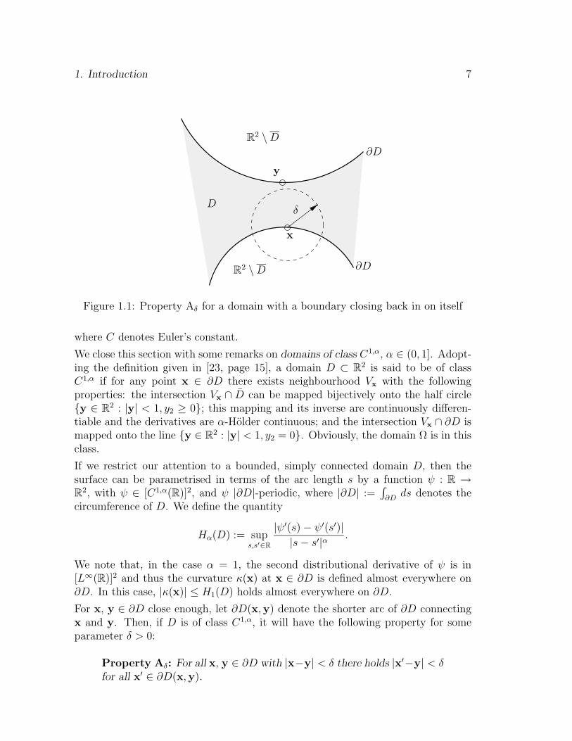
Figure 1.1: Property Aδ for a domain with a boundary closing back in on itself
where C denotes Euler’s constant.
We close this section with some remarks on domains of class C1,α, α ∈ (0, 1]. Adopt-ing the definition given in [23, page 15], a domain D ⊂ R2 is said to be of classC1,α if for any point x ∈ ∂D there exists neighbourhood Vx with the followingproperties: the intersection Vx ∩ D can be mapped bijectively onto the half circley ∈ R2 : |y| < 1, y2 ≥ 0; this mapping and its inverse are continuously differen-tiable and the derivatives are α-Holder continuous; and the intersection Vx ∩ ∂D ismapped onto the line y ∈ R2 : |y| < 1, y2 = 0. Obviously, the domain Ω is in thisclass.
If we restrict our attention to a bounded, simply connected domain D, then thesurface can be parametrised in terms of the arc length s by a function ψ : R →R
2, with ψ ∈ [C1,α(R)]2, and ψ |∂D|-periodic, where |∂D| :=∫∂D
ds denotes thecircumference of D. We define the quantity
Hα(D) := sups,s′∈R
|ψ′(s)− ψ′(s′)||s− s′|α
.
We note that, in the case α = 1, the second distributional derivative of ψ is in[L∞(R)]2 and thus the curvature κ(x) at x ∈ ∂D is defined almost everywhere on∂D. In this case, |κ(x)| ≤ H1(D) holds almost everywhere on ∂D.
For x, y ∈ ∂D close enough, let ∂D(x,y) denote the shorter arc of ∂D connectingx and y. Then, if D is of class C1,α, it will have the following property for someparameter δ > 0:
Property Aδ: For all x, y ∈ ∂D with |x−y| < δ there holds |x′−y| < δfor all x′ ∈ ∂D(x,y).
8 The Scattering of Elastic Waves by Rough Surfaces
In Figure 1.1, this property is illustrated for a domain with a boundary that closesback in on itself. Particularly, the parameter δ has to be chosen such that a circleof radius δ around any point x ∈ ∂D contains only one connected part of ∂D.
At certain points in the arguments, we will want to show certain estimates holdwith the same constants for all bounded, simply connected domains of class C1,α
that share certain geometrical properties. For this purposes, for α ∈ (0, 1], and κ0,δ, M > 0 define
Dα,κ0,δ,M := D ⊂ R2 of class C1,α, simply connected and bounded,
D satisfies Aδ, Hα(D) < κ0, |∂D| < M.
Similarily, certain results will be shown uniformly with respect to classes of functionsf defining the boundary ∂Ω. Thus, for α ∈ (0, 1], c ∈ R and M > 0, define
Bα,c,M := f ∈ C1,α(R) : ‖f‖1,α;R ≤M and inf f ≥ c.
Chapter 2
Time Harmonic Waves inLinearized Elasticity
The basis of the present investigation into scattering of elastic waves by roughsurfaces is the theory of linearized elasticity. In this chapter, we will present thefundamental equations of this theory and derive the Navier equation which governsthe propagation of time-harmonic waves in an elastic medium. The study of so-lutions to this equation is then continued by deriving regularity results up to theboundary based on regularity estimates for systems of elliptic partial differentialequations.
Subsequently we will introduce the matrices of fundamental solutions for the Navierequation in free field conditions and for a half space with a rigid boundary. Thesefundamental solutions will have a prominent role in all later chapters of this thesis,as they are at the heart of the definition of elastic potentials and also of the newradiation condition to be introduced in Chapter 4.
2.1 Linearized Elasticity Theory
The propagation of waves in an elastic solid with Lame constants µ, λ (µ > 0,λ+ µ ≥ 0) and density ρ in three-dimensional space is governed by Hooke’s law
σjk = λ div u δjk + µ
(∂uj∂xk
+∂uk∂xj
), j, k = 1, 2, 3, (2.1)
and, in the absence of exterior forces, by the equations of motion
3∑k=1
∂σjk∂xk
− ρ ∂2uj∂t2
= 0, j = 1, 2, 3. (2.2)
10 The Scattering of Elastic Waves by Rough Surfaces
Here, the vector field u denotes the displacement and (σjk) the stress tensor in R3.We will assume that the density ρ is constant throughout the medium, say ρ ≡ 1.
Throughout, only time-harmonic waves with circular frequency ω > 0 will be con-sidered, i. e. all fields are assumed to have a time dependence e−iωt. It is common tosuppress this time dependence and then, using the same symbols as before, equation(2.2) can be rewritten as
3∑k=1
∂σjk∂xk
+ ω2 uj = 0, j = 1, 2, 3. (2.3)
Inserting the components of (σjk) as given by (2.1) into (2.3) then yields the Navierequation
µ∆u + (λ+ µ) grad div u + ω2 u = 0. (2.4)
Throughout this thesis, we will be considering scattering surfaces which are invariantin one coordinate direction, say in the direction of the x3-axis, and we will alsoassume that all waves are propagating perpendicular to that direction, i. e. thefields do not depend on x3. In these situations, the system (2.4) separates into atwo-dimensional system and a scalar equation: Defining u := (u1, u2)>, we obtain
µ∆u + (λ+ µ) grad div u + ω2 u = 0, (2.5)
∆u3 +ω2
µu3 = 0. (2.6)
Equation (2.6) is, of course, the Helmholtz equation; the analysis of this equationis well understood and we shall not consider it here. For the special case of 2Dscattering by rough surfaces we refer the reader to the papers [15, 19, 20] and thereferences contained therein.
Equation (2.5) is again of the same form as (2.4), only now in two dimensions. It isin the form (2.5) that we will consider the Navier equation from now on, replacingthe notation u by u again, for convenience: the scattering problem will be treatedas a problem of plane strain. For simplicity, we also introduce the notation
∆∗u := µ∆u + (λ+ µ) grad div u.
Because of the assumptions on the Lame constants (µ > 0 and λ + µ ≥ 0), it iseasy to show that the Navier equation is uniformly strictly elliptic in any domainin R2. Thus we have the following regularity result, which shall be used extensivelywithout further reference:
Lemma 2.1 Let Ω denote a domain in R2 and u ∈ [C2(Ω)]2 a solution to theNavier equation. Then u ∈ [C∞(Ω)]2.
2. Time Harmonic Waves in Linearized Elasticity 11
Proof: The assertion follows from L2-estimates in [26] and subsequent applicationsof Sobolev’s imbedding theorem.
An important tool in the analysis of the Navier equation are the Lame potentials.We introduce the wave numbers for compressional and shear waves,
kp :=ω√
2µ+ λand ks :=
ω√µ
respectively and define the Lame potentials by
Ψp := − 1
k2p
div u and Ψs := − 1
k2s
div⊥ u. (2.7)
Some important properties of these potentials are listed in the following lemma.
Lemma 2.2 Let Ω denote a domain in R2 and u ∈ [C2(Ω)]2 a solution to theNavier equation. Then,
∆ Ψp + k2pΨp = 0,
∆ Ψs + k2sΨs = 0,
andu = grad Ψp + grad⊥Ψs.
Proof: We recalldiv ∆u = ∆ div u = div grad div u.
Thus, by applying div · to (2.4), we obtain
(2µ+ λ) ∆ div u + ω2 div u = 0.
The analogous equation for Ψs is obtained by applying div⊥ · and noting thatdiv⊥ grad div u = 0 for any three times continuously differentiable vector field. Fi-nally, we have that
∆u− grad div u = grad⊥ div u,
and thus, by (2.4),
u = − µ
ω2∆u− λ+ µ
ω2grad div u
= − 1
k2s
∆ u− 1
k2p
grad div u +1
k2s
grad div u
= − 1
k2p
grad div u− 1
k2s
grad⊥ div⊥ u.
This completes the proof.

12 The Scattering of Elastic Waves by Rough Surfaces
Remark 2.3 The vector fields up := grad Ψp and us := grad⊥Ψs are called thecompressional and shear parts of u respectively. This terminology is justified byobserving that div⊥ up = 0 and div us = 0, i.e. up is irrotational and us is divergencefree.
We follow Kupradze [35] in introducing a generalised stress tensor (πjk) by
πjk := λ div u δjk + µ∂uj∂xk
+ µ∂uk∂xj
,
where µ, λ are real numbers satisfying µ+ λ = λ+µ. In the case µ = µ and λ = λ,the generalised stress tensor is identical to the standard stress tensor (σjk).
Given a curve Λ ⊂ R2 with unit normal n, the generalised stress vector on Λ isdefined by
Pu := (πjk) n = (µ+ µ)∂u
∂n+ λn div u− µn⊥ div⊥ u.
This notion has also been used in the papers [25, 38] and its 3D equivalent in [31].Its significance and its properties for a special choice of µ and λ will be discussed indetail in Chapter 3 when we discuss the properties of elastic single- and double-layerpotentials. For now, we only point out that Pu is equal to the physical stress vectorTu for the choice µ = µ and λ = λ.
Using the generalised stress vector, the generalised Betti formulae result as a con-sequence of the divergence theorem:
Lemma 2.4 Let B ⊆ R2 be a domain in which the divergence theorem holds andlet n denote the outward drawn normal on ∂B. Then, for vector fields v ∈ [C1(B)]2
and w ∈ [C2(B)]2, the first generalised Betti formula holds:∫B
v ·∆∗w dx =
∫∂B
v ·Pw ds−∫B
Eµ,λ(v,w) dx, (2.8)
where
Eµ,λ(v,w) := (2µ+ λ)
(∂v1
∂x1
∂w1
∂x1
+∂v2
∂x2
∂w2
∂x2
)+ µ
(∂v1
∂x2
∂w1
∂x2
+∂v2
∂x1
∂w2
∂x1
)+ λ
(∂v1
∂x1
∂w2
∂x2
+∂v2
∂x2
∂w1
∂x1
)+ µ
(∂v1
∂x2
∂w2
∂x1
+∂v2
∂x1
∂w1
∂x2
).
For v ∈ [C2(B)]2 the second generalised Betti formula holds:∫B
v ·∆∗v dx =
∫∂B
v ·Pv ds−∫B
Eµ,λ(v,v) dx. (2.9)
Finally, for v, w ∈ [C2(B)]2 the third generalised Betti formula holds:∫B
(v ·∆∗w −∆∗ v ·w) dx =
∫∂B
(v ·Pw −Pv ·w) ds. (2.10)
Proof: As in Kupradze [35] for the three-dimensional case.

2. Time Harmonic Waves in Linearized Elasticity 13
2.2 Regularity of Solutions
For many of the subsequent considerations, we will need regularity results for solu-tions to the Navier equation and their derivatives in domains with smooth bound-aries. Appendix A gives proofs of such results for weak solutions to elliptic systems.In this section, we will use these results to obtain regularity estimates up to theboundary for classical solutions to the Navier equation that are also weak solutions.
Let us start with a simple interior estimate, however:
Lemma 2.5 Given a domain G ⊂ R2, let u ∈ [L∞(G)]2 be a solution to the Navierequation (2.4) in G in a distributional sense. Assume G′ ⊂⊂ G and set d :=d(∂G′, ∂G). Then, u ∈ [C1(G′)]2 and for all x ∈ G′,
|graduk(x)| ≤ C (1 + d−1) ‖u‖∞;G (k = 1, 2),
where C is only dependent on µ, λ and ω.
Proof: Application of estimates in Fichera [26] and Sobolev’s Imbedding Theorem.
By applications of this result we immediately obtain the following corollary:
Corollary 2.6 Given a domain G ⊂ R2, let (vn) ⊂ [L∞(G)]2 be a sequence of
solutions to the Navier equation in G and, for some vector field v, suppose thatvn(x) → v(x) uniformly on compact subsets of G. Then v ∈ [C2(G)]2 and is asolution to the Navier equation in G.
Now we want to establish regularity up to the boundary, using the results of Ap-pendix A. Given a compact subdomain D of Ω and following Definition A.1, avector field u ∈ [H1(D)]2 is said to be a weak solution to the Navier equation if, forany test field v ∈ [H1
0 (D)]2, the equation
∫D
µ
2∑j=1
graduj · grad vj + (λ+ µ) div u div v − ω2 u · v
dx = 0
holds (see also [46]).
To apply the regularity results derived in the appendix to classical solutions to theNavier equation in Ω, we now construct a set of bounded sub-domains of class C1,α
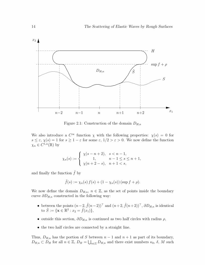
by the following procedure (illustrated in Figure 2.1). We set , for some H > sup f ,
ρ :=H − sup f
3.
14 The Scattering of Elastic Waves by Rough Surfaces
n−2 n−1 n n+1 n+2
DH,n
x1
x2
S
S
sup f + ρ
H
Figure 2.1: Construction of the domain DH,n
We also introduce a C∞ function χ with the following properties: χ(s) = 0 fors ≤ ε, χ(s) = 1 for s ≥ 1− ε for some ε, 1/2 > ε > 0. We now define the functionχn ∈ C1,α(R) by
χn(s) :=
χ(s− n+ 2), s < n− 1,
1, n− 1 ≤ s ≤ n+ 1,χ(n+ 2− s), n+ 1 < s,
and finally the function f by
f(s) := χn(s) f(s) + (1− χn(s)) (sup f + ρ).
We now define the domain DH,n, n ∈ Z, as the set of points inside the boundarycurve ∂DH,n constructed in the following way:
• between the points (n−2, f(n−2))> and (n+2, f(n+2))>, ∂DH,n is identicalto S := x ∈ R2 : x2 = f(x1),
• outside this section, ∂DH,n is continued as two half circles with radius ρ,
• the two half circles are connected by a straight line.
Thus, DH,n has the portion of S between n − 1 and n + 1 as part of its boundary,DH,n ⊂ DH for all n ∈ Z, DH =
⋃n∈ZDH,n and there exist numbers κ0, δ, M such

2. Time Harmonic Waves in Linearized Elasticity 15
that DH,n ∈ Dα,κ0,δ,M for all n ∈ Z. Moreover, as for x, y ∈ DH with |x − y| ≤ 1there always exists a number n0 ∈ Z such that x, y ∈ DH,n0 , it follows that there isa constant C, only depending on α, such that
‖u‖1,α;DH ≤ C supn∈Z‖u‖1,α;DH,n
for any u ∈ C1,α(DH). Thus we can now apply the regularity results stated inTheorem A.12 to classical solutions of the Navier equation.
Theorem 2.7 Let u ∈ [C2(Ω)∩C(Ω)∩H1loc(Ω)]2 be a solution to the Navier equation
in Ω, bounded in DH for all H > sup f , and u = 0 on S. Then u ∈ V1,α(Ω) and,for any H > sup f , u ∈ C1,α(DH) with
‖u‖1,α;DH ≤ C ‖u‖0;DH , (2.11)
where C is a constant only depending on λ, µ, ω, H, α, κ0, δ and M .
Proof: Apply Theorem A.12 with D′ = DH,n for all n ∈ Z.
2.3 The Free-Field Green’s Tensor
Central to potential theory is the idea of fundamental solutions; in the case of theNavier equation, matrices of fundamental solutions (MFS) fulfill the same role. Thek-th column of an MFS, M, to the Navier equation is a solution to the equation
∆∗xM·k(x,y) + ω2M·k(x,y) = −δ(x− y) ek, k = 1, 2,
for x, y ∈ D for some domain D ⊂ R2, where δ denotes Dirac’s delta distributionand ek the k-th cartesian unit coordinate vector. The MFS most commonly used inconjunction with the Navier equation is the free field Green’s tensor Γ given by
Γ(x,y) :=i
4µH
(1)0 (ks|x− y|) I +
i
4ω2∇>x∇x
(H
(1)0 (ks|x− y|)−H(1)
0 (kp|x− y|)),
(2.12)
with x, y ∈ R2, x 6= y, where H(1)n (·) denotes the Hankel function of the first kind
and of order n.
As, for example, Kress points out [34], with the help of the Bessel differentialequation it is easy to see that the components of this matrix can be written as
Γjk(x,y) =i
4µ
Φ1(|x− y|) δjk + Φ2(|x− y|) (xj − yj)(xk − yk)
|x− y|2
(j, k = 1, 2),
(2.13)
16 The Scattering of Elastic Waves by Rough Surfaces
where, introducing the constant τ = kp/ks,
Φ1(t) := H(1)0 (kst)−
1
ks t
(H
(1)1 (kst)− τ H(1)
1 (kpt)),
Φ2(t) :=2
ks tH
(1)1 (kst)−H(1)
0 (kst)−2τ
ks tH
(1)1 (kpt) + τ 2 H
(1)0 (kpt).
This formulation is very convenient to analyse the singular behaviour of Γ as |x −y| → 0 by applying (1.6). This behaviour and some other well known basic proper-ties of Γ are given in the following theorem.
Theorem 2.8 The MFS Γ is analytic for x 6= y. It is symmetric, its columns androws are solutions to the Navier equation with respect to x in R2 \ y and withrespect to y in R2 \ x. Furthermore, it satisfies, for some constant C > 0, theestimate
maxj,k=1,2
|Γjk(x,y)| ≤ C (1 + | log |x− y| |) . (2.14)
The Lame potential representation of the columns of Γ is given by
Γ·k(x,y) = gradx Ψ(k)p (x,y) + grad⊥x Ψ(k)
s (x,y), k = 1, 2, (2.15)
where
Ψ(1)p (x,y) := − i
4ω2
∂
∂x1
H(1)0 (kp|x− y|), (2.16)
Ψ(2)p (x,y) := − i
4ω2
∂
∂x2
H(1)0 (kp|x− y|), (2.17)
Ψ(1)s (x,y) := − i
4ω2
∂
∂x2
H(1)0 (ks|x− y|), (2.18)
Ψ(2)s (x,y) := +
i
4ω2
∂
∂x1
H(1)0 (ks|x− y|). (2.19)
Using Fourier transforms, we can obtain an alternative representation of Γ whichwill be useful in the next section. For functions f depending on x1 and y1 throughthe difference X1 = x1 − y1, we will temporarily denote by F [f ] or alternatively byf the Fourier transform with respect to X1 := x1 − y1, i.e.
F [f ](t) = f(t) =
∫ ∞−∞
f(X1) eiX1t dX1.
It is well known that
F [H(1)0 (k|x− y|) ](t) =
2 ei√k2−t2|x2−y2|√k2 − t2
, (2.20)
2. Time Harmonic Waves in Linearized Elasticity 17
where the branches of the square root function in the complex plane are chosen suchthat the imaginary part is non-negative. This will be the convention throughoutthe thesis. We introduce the notations
γp :=√k2p − t2 and γs :=
√k2s − t2.
Calculating the Fourier transforms of (2.16)–(2.19) using (2.20) and inserting theresult in (2.15) then yields
F [ Γ(x,y) ](t) =i
2ω2
(t2/γp −t sgn(x2 − y2)
−t sgn(x2 − y2) γp
)eiγp|x2−y2|
+
(γs t sgn(x2 − y2)
t sgn(x2 − y2) t2/γs
)eiγs|x2−y2|
. (2.21)
By applying the generalised stress operator P to Γ, we obtain matrix functions Π(1)
and Π(2):
Π(1)jk (x,y) :=
(P(x)(Γ·k(x,y))
)j,
Π(2)jk (x,y) :=
(P(y)(Γj·(x,y))>
)k.
The properties of these matrix functions, very similar to those of Γ, are listed in thefollowing theorem.
Theorem 2.9
(a) For y ∈ R2, the columns of Π(2)(·,y) are solutions to the Navier equation (2.4)in R2 \ y.
(b) For x ∈ R2, the rows of Π(1)(x, ·) are solutions to the Navier equation (2.4)in R2 \ x.
(c) For x, y ∈ R2, x 6= y, there holds
Π(2)(x,y) = Π(1)(y,x)>.
(d) Let B ⊆ R2 be a bounded domain in which the divergence theorem holds. Thenany solution u ∈ C2(B) to the Navier equation can be represented as
u(x) =
∫∂B
Γ(x,y) Pu(y)− Π(2)(x,y) u(y) ds(y)
for all x ∈ B.
18 The Scattering of Elastic Waves by Rough Surfaces
Proof: Part (c) follows directly from the definitions of Π(j) (j = 1, 2) and P togetherwith Theorem 2.8. The same argument yields that the columns of Π(2)(·,y) aresolutions to the Navier equation in R2 \ y.
Part (b) is now a direct consequence of parts (a) and (c).
Part (d) is finally seen by applying the 3rd generalised Betti formula (2.10) and astandard potential theoretic argument, using the fact that Γ(x,y) has a logarithmicsingularity for |x− y| → 0.
2.4 The Green’s Tensor for the First Boundary
Value Problem in a Half Space
As was pointed out in the introduction, and can be proven rigorously from (2.13),the free field Green’s tensor Γ satisfies (1.3) only for p = 1/2. This asymptotic decayrate as |x− y| → ∞ is not sufficient to ensure that integrals of the type∫
S
Γ(x,y)φ(y) ds(y)
exist for all φ ∈ [BC(S)]2. Therefore, we will derive and analyse the Green’s tensorΓD,h for the first boundary value problem of elasticity in a half space Uh (h ∈ R).This Green’s tensor was first introduced in [4]; this section gives a more detailedpresentation of the results of that paper.
Motivated by the form of the corresponding Green’s function for acoustical wavepropagation, we make an ansatz of the form
ΓD,h(x,y) = Γ(x,y)− Γ(x,y′h) + U(x,y), x,y ∈ Uh,x 6= y, (2.22)
with a yet unknown matrix function U. In fact, we will assume that U only dependson x and y through the variables X1 = x1 − y1, x2 and y2. For fixed y ∈ Uh, thecolumns of U(·,y) have to satisfy
∆∗xU·,k(x,y) + ω2U·,k(x,y) = 0, x ∈ Uh \ y,U·,k(x,y) = −Γ·k(x,y) + Γ·k(x,y
′h), x ∈ ∂Uh,
and they also have to be bounded and represent a wave field propagating away fromTh (this notion will be made mathematically precise in Chapter 4 when we discussradiation conditions).
We represent U by its Lame potentials,
U·k(x,y) = gradx Ψ(k)U,p(x,y) + grad⊥x Ψ
(k)U,s(x,y), k = 1, 2, (2.23)
2. Time Harmonic Waves in Linearized Elasticity 19
and conclude by Lemma 2.2 that
∆xΨ(k)U,p(x,y) + k2
pΨ(k)U,p(x,y) = 0 and ∆xΨ
(k)U,s(x,y) + k2
sΨ(k)U,p(x,y) = 0.
Taking the Fourier transform with respect to X1, we obtain the two ordinary differ-ential equations
d2
dx22
Ψ(k)U,p + γ2
p Ψ(k)U,p = 0 (2.24)
andd2
dx22
Ψ(k)U,s + γ2
s Ψ(k)U,s = 0 (2.25)
As it is assumed that U be bounded and represent an outgoing wave field, we selectsolutions to these equations of the form
Ψ(k)U,p = A(k)
p (t, y2) eiγp(x2−h) and Ψ(k)U,s = A(k)
s (t, y2) eiγs(x2−h). (2.26)
The coefficient functions A(k)p and A
(k)s can now be calculated from the boundary
conditions. Using (2.21), we obtain, for x2 = h,
−itΨ(1)U,p +
d
dx2
Ψ(1)U,s = 0,
d
dx2
Ψ(1)U,p + itΨ
(1)U,s =
it
ω2
(eiγp(y2−h) − eiγs(y2−h)
),
−itΨ(2)U,p +
d
dx2
Ψ(2)U,s =
it
ω2
(eiγp(y2−h) − eiγs(y2−h)
),
d
dx2
Ψ(2)U,p + itΨ
(2)U,s = 0.
Inserting the solutions (2.26) yields, after some elementary calculations,(A
(1)p A
(1)s
A(2)p A
(2)s
)(t, y2) = − 1
ω2 (γpγs + t2)
(tγs t2
−t2 tγp
)(eiγp(y2−h) − eiγs(y2−h)
).
Now, taking inverse Fourier transforms and using (2.23), we finally arrive at
U(x,y) = − i
2πω2
∫ ∞−∞
(Mp(t, γp, γs;x2, y2) +Ms(t, γp, γs;x2, y2)) e−iX1t dt, (2.27)
with
Mp(t, γp, γs;x2, y2) :=eiγp(x2+y2−2h) − ei(γp(x2−h)+γs(y2−h))
γpγs + t2
(−t2γs t3
tγpγs −t2γp
),
Ms(t, γp, γs;x2, y2) :=eiγs(x2+y2−2h) − ei(γs(x2−h)+γp(y2−h))
γpγs + t2
(−t2γs −tγpγs−t3 −t2γp
).
From the construction of U, we immediately have the following theorem, listingsome basic properties of ΓD,h:
20 The Scattering of Elastic Waves by Rough Surfaces
Theorem 2.10 For y ∈ Uh, ΓD,h(·,y) − Γ(·,y) ∈ [C∞(Uh) ∩ C1(Uh)]2×2, and the
columns of ΓD,h(·,y) are solutions to the Navier equation (2.4) in Uh \ y. Fur-thermore, ΓD,h(x,y) = 0 for x ∈ ∂Uh.
We will now address the main advantage of using ΓD,h over Γ in rough surfacescattering applications, its faster asymptotic decay rate as |x1| → ∞ in horizontallayers above ∂Uh. For the first two terms in its representation, this is shown in thefollowing lemma:
Lemma 2.11 For x, y ∈ Uh, |x− y| ≥ 1 the estimate
maxj,k=1,2
|Γjk(x,y)− Γjk(x,y′h)| ≤
H(x2 − h, y2 − h)
|x− y|3/2,
holds, where H ∈ C(R2).
Proof: Using (2.13) and the notations r = |x− y| and r′ = |x− y′h|, there holds
Γ(x,y)− Γ(x,y′h) =i
4µ
(Φ1(r)− Φ1(r′)) I
+
(0 2(2h− y2)(x1 − y1)
2(2h− y2)(x1 − y1) 0
)Φ2(r)
r2
+
((x1 − y1)2 (x1 − y1)(x2 + y2 − 2h)
(x1 − y1)(x2 + y2 − 2h) (x2 + y2 − 2h)2
)(Φ2(r)
r2− Φ2(r′)
r′2
).
So it obviously suffices to show the estimate for the functions
Φ1(r)− Φ1(r′),(x1 − y1)Φ2(r)
r2, and (x1 − y1)2
(Φ2(r)
r2− Φ2(r′)
r′2
).
Using the mean value theorem yields
|Φ1(r)− Φ1(r′)| ≤ |r − r′| maxr≤t≤r′
|Φ′1(t)| = 4(x2 − h)(y2 − h)
r + r′maxr≤t≤r′
|Φ′1(t)|
and thus the asymptotic decay rate of Hankel functions and their derivatives (1.5)yields the asserted estimate in the first case because of the assumption |x− y| ≥ 1.
In the second case, x1−y1
ris bounded and Φ2(r)
rhas the required decay rate. For the
last function, we rewrite
Φ2(r)
r2− Φ2(r′)
r′2=
(Φ2(r)− Φ2(r′) + 4(x2−h)(y2−h)
r2 Φ2(r))
r2 + 4(x2 − h)(y2 − h).

2. Time Harmonic Waves in Linearized Elasticity 21
−kp−ks 0
kp ks
branch cuts
path of integration
C1 C2 C3 C4
Im(t)
Re(t)
Figure 2.2: The path of integration
Now, (x1−y1)2
r2+4(x2−h)(y2−h)is bounded, Φ2(r)− Φ2(r′) can be estimated in the same way
as Φ1(r)− Φ1(r′) above and Φ2(r)r2 decays even faster than required.
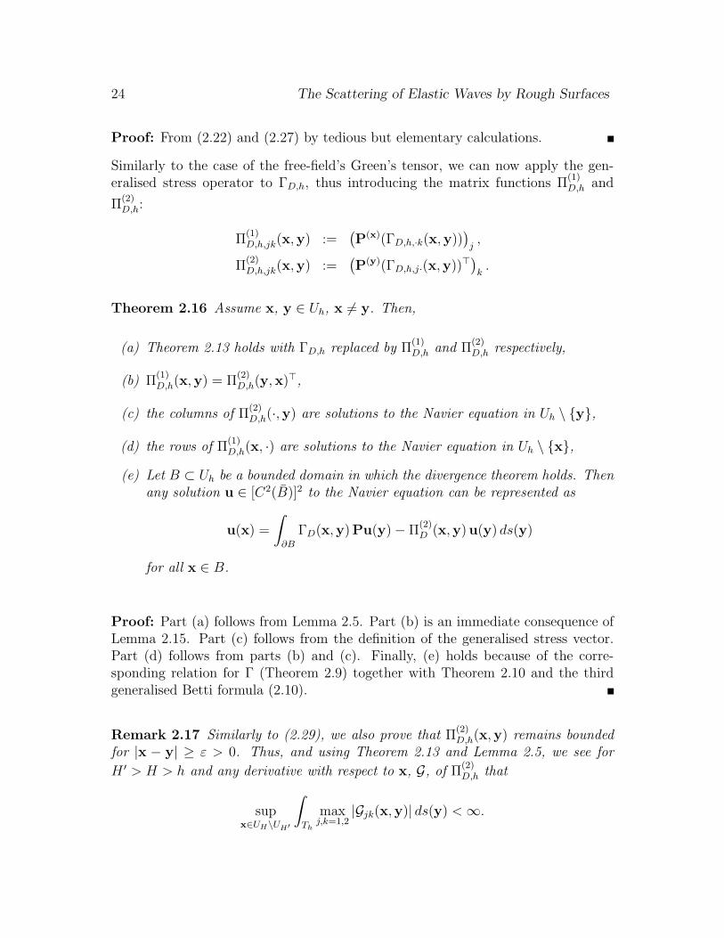
To prove a similar estimate for U, a more lengthy analysis is required. To obtainalternative representations of the integrals used in (2.27), we deform the path ofintegration in the complex plane. To this end, branch cuts from ±kp and ±ks,respectively to ±kp ± i∞ and ±ks ± i∞, are introduced. Recall that the branchesof the analytic extensions of γp and γs were chosen such that their imaginary part isnon-negative. Note also that the integrands in (2.27) do not have any singularitieson the chosen branches of γp and γs. Restricting ourselves to the case x1 > y1 for themoment, we deform the path of integration into the lower half plane as illustratedin Figure 2.2.
It is easily seen that the integrals over the arcs vanish as their radius tends toinfinity, so only the branch line integrals remain. Denoting the paths of integrationalong the branch cuts by C1 ∪ C2 and C3 ∪ C4, as indicated in Figure 2.2, we rewriteU as
U(x,y) = I1 + I2 + I3 + I4, (2.28)
22 The Scattering of Elastic Waves by Rough Surfaces
with
I1 := − i
2πω2
∫C1∪C2
Mp(t, γp, γs;x2 − h, y2 − h) e−iX1t dt,
I2 := − i
2πω2
∫C1∪C2
Ms(t, γp, γs;x2 − h, y2 − h) e−iX1t dt,
I3 := − i
2πω2
∫C3∪C4
Mp(t, γp, γs;x2 − h, y2 − h) e−iX1t dt,
I4 := − i
2πω2
∫C3∪C4
Ms(t, γp, γs;x2 − h, y2 − h) e−iX1t dt.
More explicitly, there holds
I1 = − i
2πω2eiX1ks
∫ ∞0
Mp(−ks−is, γp|C2 , γs|C2 ;x2 − h, y2 − h)
−Mp(−ks−is, γp|C1 , γs|C1 ;x2 − h, y2 − h)e−X1s ds,
and similar formulae for the other three integrals. Note that γs|C2 = −γs|C1 , andγp|C1 = γp|C2 . Using the mean-value theorem, we thus conclude
Mp(−ks−is, γp|C2 , γs|C2 ;x2, y2)−Mp(−ks−is, γp|C1 , γs|C1 ;x2, y2)
= 2 Re(γs|C1)∂Mp
∂γs(−ks−is, γp|C1 , ξ;x2, y2)
for some ξ on the line between γs|C1 and γs|C2 . Now, ∂Mp
∂γs(−ks−is, γp|C1 , ξ;x2, y2) is seen
to be continuously dependent on s in [0,∞) and, for some constant C continuouslydependent on x2 and y2, there holds∣∣∣∣s−1/2 Re(γs|C2)
∂M
∂γs(−ks−is, γp|C1 , ξ;x2, y2)
∣∣∣∣ ≤ C
for s ∈ [0, 1]. Therefore, we can estimate the asymptotic decay rate of I1 by em-ploying the following lemma with r = 1
2.
Lemma 2.12 Assume q ∈ C([0,∞)) such that C1 :=∫∞
0|q(s)|e−s ds exists. For
X > 1, set
I(X) :=
∫ ∞0
q(s) e−Xs ds.
Further assume that for some r > −1 there exists C2 > 0 with |s−rq(s)| ≤ C2 forall s ∈ [0, 1]. Then, for X ≥ 1 + (r + 1) logX,
|I(X)| ≤ (C1 + Γ(r + 1)C2)1
Xr+1.
2. Time Harmonic Waves in Linearized Elasticity 23
Proof: We can estimate∣∣∣∣∫ 1
0
q(s) e−Xs ds
∣∣∣∣ ≤ C2
∫ 1
0
sre−Xs ds ≤ C2Γ(r + 1)
Xr+1.
On the other hand, we have∣∣∣∣∫ ∞1
q(s) e−Xs ds
∣∣∣∣ ≤ e−(X−1)
∫ ∞1
|q(s)|e−s ds ≤ C1
Xr+1
for all X ≥ 1 + (r + 1) logX. Adding these two estimates yields the assertion.
An identical analysis yields this decay rate for the other three integrals in (2.28)and also for the case x1 < y1. In the latter case the path of integration has to bedeformed into the upper half plane. Thus, also recalling Lemma 2.11, the followingtheorem is proved:
Theorem 2.13 For x,y ∈ Uh, ε > 0 and |x1 − y1| ≥ ε, the estimate
maxj,k=1,2
|ΓD,h,jk(x,y)| ≤ H(x2 − h, y2 − h)
|x1 − y1|3/2
holds, where H ∈ C(R2).
Remark 2.14 We also note that from (2.14) together with Theorem 2.13, we seethat there exists some constant C > 0 such that
maxj,k=1,2
|ΓD,h,jk(x,y)| ≤ C |1 + log |x− y| | (2.29)
for x, y ∈ Uh. As a consequence, together with an application of Theorem 2.13, wehave, for h < inf f and h′ > sup f , that
supx∈Dh′
∫S
maxj,k=1,2
|ΓD,h,jk(x,y)|2 ds(y) <∞.
For much of the subsequent arguments, the following lemma will be useful:
Lemma 2.15 For x, y ∈ Uh, x 6= y, the following reciprocity relation holds:
ΓD,h(x,y) = ΓD,h(y,x)>.
24 The Scattering of Elastic Waves by Rough Surfaces
Proof: From (2.22) and (2.27) by tedious but elementary calculations.
Similarly to the case of the free-field’s Green’s tensor, we can now apply the gen-eralised stress operator to ΓD,h, thus introducing the matrix functions Π
(1)D,h and
Π(2)D,h:
Π(1)D,h,jk(x,y) :=
(P(x)(ΓD,h,·k(x,y))
)j,
Π(2)D,h,jk(x,y) :=
(P(y)(ΓD,h,j·(x,y))>
)k.
Theorem 2.16 Assume x, y ∈ Uh, x 6= y. Then,
(a) Theorem 2.13 holds with ΓD,h replaced by Π(1)D,h and Π
(2)D,h respectively,
(b) Π(1)D,h(x,y) = Π
(2)D,h(y,x)>,
(c) the columns of Π(2)D,h(·,y) are solutions to the Navier equation in Uh \ y,
(d) the rows of Π(1)D,h(x, ·) are solutions to the Navier equation in Uh \ x,
(e) Let B ⊂ Uh be a bounded domain in which the divergence theorem holds. Thenany solution u ∈ [C2(B)]2 to the Navier equation can be represented as
u(x) =
∫∂B
ΓD(x,y) Pu(y)− Π(2)D (x,y) u(y) ds(y)
for all x ∈ B.
Proof: Part (a) follows from Lemma 2.5. Part (b) is an immediate consequence ofLemma 2.15. Part (c) follows from the definition of the generalised stress vector.Part (d) follows from parts (b) and (c). Finally, (e) holds because of the corre-sponding relation for Γ (Theorem 2.9) together with Theorem 2.10 and the thirdgeneralised Betti formula (2.10).
Remark 2.17 Similarly to (2.29), we also prove that Π(2)D,h(x,y) remains bounded
for |x − y| ≥ ε > 0. Thus, and using Theorem 2.13 and Lemma 2.5, we see for
H ′ > H > h and any derivative with respect to x, G, of Π(2)D,h that
supx∈UH\UH′
∫Th
maxj,k=1,2
|Gjk(x,y)| ds(y) <∞.
Chapter 3
Elastic Potentials on RoughSurfaces
It is the object of this chapter to establish regularity results for elastic poten-tials defined on the surface S and mapping properties of related integral operators.Throughout this chapter, we will limit ourselves to surfaces given as the graph offunctions f ∈ C1,1(R). To be able to establish our final results, we will point out aspecial choice of the values µ and λ in the definition of the generalised stress vector,for which the kernel in the definition of the double-layer potential only has a weaksingularity for x→ y on S. We will then restate some well known properties of theelastic potentials in the case of a closed boundary curve. These results will differfrom the usual formulation, however, in that emphasis will be laid on uniformitywith respect to a certain class of boundary curves. Returning to the case of theunbounded surface S, the results for the closed boundary curve will be applied bydecomposing the potentials into a smooth part defined on all of S and a singularpart with support only on a compact subset of S. Thus we derive similar regularityresults for the rough surface potentials.
3.1 Basic Properties of Elastic Potentials
We will start this chapter by introducing the elastic potentials of interest to us. Fora vector valued density φ ∈ [BC(S)]2, we define an elastic single-layer potential onthe rough surface S by
v(x) :=
∫S
ΓD,h(x,y)φ(y) ds(y) for x ∈ Uh \ S, (3.1)
26 The Scattering of Elastic Waves by Rough Surfaces
and a double-layer potential on S by
w(x) :=
∫S
Π(2)D,h(x,y)φ(y) ds(y) for x ∈ Uh \ S. (3.2)
If we assume D to be a bounded, simply connected domain of class C1,1, we similarlycan, for φ ∈ [C(∂D)]2, define a single-layer potential on ∂D by
vD(x) :=
∫∂D
Γ(x,y)φ(y) ds(y), x ∈ R2 \ ∂D, (3.3)
and the elastic double-layer potential
wD(x) :=
∫∂D
Π(2)(x,y)φ(y) ds(y), x ∈ R2 \ ∂D. (3.4)
From the properties of the fundamental solutions Γ and ΓD,h as well as their deriva-
tives Π(2) and Π(2)D,h, it is clear that all the integrals exist as improper integrals.
Furthermore, the following theorem is a standard result:
Theorem 3.1 The potentials v and w are solutions to the Navier equation in Uh\Ωand in Ω. The potentials vD and wD are solutions to the Navier equation in D andin R2 \ D.
3.2 The Pseudo Stress Operator
In Section 2.1 the generalised stress operator P was introduced. We will now inves-tigate what influence the parameters µ and λ in its definition have on the singularbehaviour of the derivatives of the fundamental solution, Π(j)(x,y), j = 1, 2, for|x − y| → 0. We will find that for the special choice µ = µ (µ + λ)/(3µ + λ) andλ = (2µ + λ)(µ + λ)/(3µ + λ), these matrix functions become weakly singular. Inthis case, P is called the pseudo stress operator (Kupradze [35]).
To simplify the investigations, we introduce Kelvin’s matrix, the matrix of funda-mental solutions for elasto-static problems, i.e. boundary value problems involvingthe Navier equation with ω = 0:
ΓK(x,y) :=3µ+ λ
4π µ (2µ+ λ)log
1
|x− y|I +
µ+ λ
4π µ (2µ+ λ)J(x− y),
for x, y ∈ R2, x 6= y, with
J(z) :=z z>
|z|2.
As the following theorem shows, the matrix function ΓK has the same singularbehaviour as Γ itself.
3. Elastic Potentials on Rough Surfaces 27
Theorem 3.2 The matrix function ∆ defined by
∆(x,y) := Γ(x,y)− ΓK(x,y), x 6= y,
belongs to [C1(R2 × R2)]2×2.
Proof: It is only necessary to show that ∆ is well-defined and continuously differ-entiable for x = y. From (2.13) and asymptotic expansions for Φ1, Φ2 given in [34],we see that
∆(x,y) = Φ1(|x− y|) I + Φ2(|x− y|) J(x− y),
with
Φ1(t) = β1 t2 log t+ γ + log t O(t4) +O(t2),
Φ2(t) = β2 t2 log t+ log t O(t4) +O(t2)
as t→ 0, with complex constants β1, β2 and γ.
We further introduce the matrix function H(l) by
H(l)(z) := −2 zlz z>
|z|4+
el z> + z e>l|z|2
, l = 1, 2,
for z ∈ R2, where el denotes the l-th cartesian unit coordinate vector. An easycalculation then shows
∂
∂xl∆(x,y) = Φ′1(|x− y|) xl − yl
|x− y|I + Φ′2(|x− y|) xl − yl
|x− y|J(x− y)
+ Φ2(|x− y|) H(l)(x− y).
As
Φ′1(t) = 3β1 t log t+ log t O(t3) +O(t),
Φ′2(t) = 3β2 t log t+ log t O(t3) +O(t)
as t→ 0, the assertion follows.
We will now apply the generalised stress operator P(x) to the columns of ΓK . Denoteby Λ a curve of class C1,1 in R2 and by n(x) its normal at x ∈ Λ. For x ∈ Λ, y ∈ R2
and setting r := |x− y| as well as C := (3µ+ λ)/(4πµ(2µ+ λ)), we obtain
ΓK,jk(x,y) = C
δjk log
1
r+
µ+ λ
3µ+ λ
∂r
∂xj
∂r
∂xk
.
28 The Scattering of Elastic Waves by Rough Surfaces
Thus, after some calculation,
∂ΓK,jk(x,y)
∂n(x)= C
δjk
∂
∂n(x)log
1
r+
µ+ λ
3µ+ λ
2∑l=1
nl∂
∂xl
(∂r
∂xj
∂r
∂xk
)= C
∂
∂n(x)log
1
r
(δjk + 2
µ+ λ
3µ+ λ
∂r
∂xj
∂r
∂xk
)− µ+ λ
3µ+ λ
(nj
∂
∂xklog
1
r+ nk
∂
∂xjlog
1
r
).
Similarly, we obtain
divxΓK,·k =2µ
3µ+ λ
∂
∂xklog
1
r,
and thus
(n(x) divxΓK,·k)j =2µ
3µ+ λnj
∂
∂xklog
1
r.
Finally, there holds
(n⊥(x) div⊥x ΓK,·k
)j
=2∑l=1
nl
(∂ΓK,jk(x,y)
∂xl− ∂ΓK,lk(x,y)
∂xj
)= 2C
2µ+ λ
3µ+ λ
δjk
∂
∂n(x)log
1
r− nk
∂
∂xjlog
1
r
.
Combining these results yields
(P(x)(ΓK,·k(x,y))
)j
= C∂
∂n(x)log
1
r
((µ+ µ− 2µ
2µ+ λ
3µ+ λ) δjk
+ 2 (µ+ µ)µ+ λ
3µ+ λ
∂r
∂xj
∂r
∂xk
)+ C nk
∂
∂xjlog
1
r
(2µ
2µ+ λ
3µ+ λ− (µ+ µ)
µ+ λ
3µ+ λ
)+ Cnj
∂
∂xklog
1
r
(λ
2µ
3µ+ λ− (µ+ µ)
µ+ λ
3µ+ λ
). (3.5)
We thus immediately obtain the following lemma:
Lemma 3.3 Let Λ denote a curve of class C1,1 in R2 and assume x ∈ Λ, y ∈ R2.For the choice µ = µ (µ+λ)/(3µ+λ) and λ = (2µ+λ)(µ+λ)/(3µ+λ), there holds
(P(x)(ΓK,·k(x,y))
)j
=1
2π
(2µ+ λ
3µ+ λδjk + 2
µ+ λ
3µ+ λ
∂r
∂xj
∂r
∂xk
)∂
∂n(x)log
1
r.
3. Elastic Potentials on Rough Surfaces 29
Proof: Immediate from (3.5) by inserting the given expressions for µ and λ.
Remark 3.4 Let Λ denote a curve of class C1,1 in R2 and assume x, y ∈ Λ. Then,as a consequence of Theorem 3.2 and Lemma 3.3 and also observing Theorem 2.9(c), we have that the estimate (2.14) holds with Γ replaced by Π(j), j = 1, 2.
3.3 Uniform Regularity Results for Elastic Poten-
tials on Bounded Surfaces
It is the goal of this section to state regularity results and jump relations for elasticpotentials defined on smooth, bounded, closed surfaces. These results are in princi-ple well known [24,35]. In our presentation here, we will rely heavily on the proofsgiven in [24], but the results will be generalised in two important aspects. Firstly,we shall consider boundary curves of class C1,1 instead of those of class C2. Thisextension is important for the solvability theory presented in Chapter 5 as this the-ory requires a compactness property of bounded families of such surfaces in a weaktopology. This property would not be satisfied without additional equicontinuityassumptions by families of C2 surfaces.
Secondly, we shall identify the properties of the boundary curves that determine theconstants in the regularity estimates. We are thus able to formulate these resultsuniformly for classes of domains sharing these properties.
Let us address the generalisation to C1,1 boundary curves first. For a detailedanalysis of potentials defined on Lyapunov surfaces, see e.g. [29]. For a boundary∂D of class C1,1, the curvature κ(x) can be defined for allmost all x ∈ ∂D. Moreover,recalling the remarks on C1,α domains in Section 1.3, there holds κ ∈ L∞(∂D) and‖κ‖L∞(∂D) ≤ H1(D).
A careful review of the proof of the regularity estimates in [24] reveals that theassumption of a C2 boundary is only used to obtain certain geometrical estimatesthrough Taylor expansions up to second order. In the proof of the following lemma(Lemma 1.1 in [24]) we indicate how these results can be proved in the case of aboundary of class C1,1.
Lemma 3.5 For some numbers κ0, δ, M > 0, assume D ∈ D1,κ0,δ,M . Then
|n(x) · (x− y)| ≤ q |x− y|2,|n(x)− n(y)| ≤ q |x− y|
30 The Scattering of Elastic Waves by Rough Surfaces
for all x, y ∈ ∂D, with the constant q given by
q = max
√2κ0, 2(minδ, 1
2κ0
)−1, (minδ, 1
2κ0
)−2M
.
Proof: Let ∂D be parametrised in terms of its arc length and denote by t(s) andn(s) the tangent and normal vectors at s, respectively, and by κ(s) the curvatureat s, for all s where it is defined. Then
∂
∂s|x(s)− x(s0)|2 = 2 t(s) · (x(s)− x(s0)),
∂2
∂s2|x(s)− x(s0)|2 = 2 [1− κ(s) n(s) · (x(s)− x(s0))],
where the second equation holds for almost all s. Thus
|x(s)− x(s0)|2 = 2
∫ s
s0
∫ t
s0
[1− κ(t′) n(t′) · (x(t′)− x(s0)] dt′ dt,
n(s0) · (x(s)− x(s0)) = −∫ s
s0
∫ t
s0
κ(t′) n(t′) · n(s0) dt′ dt.
First suppose that |x(s) − x(s0)| ≤ minδ, (2κ0)−1. Then an easy estimate of thedouble integral in the first equation yields
|x(s)− x(s0)|2 ≥ 1
2(s− s0)2,
and consequently, from the second equation,
|n(s0) · (x(s)− x(s0))| ≤ κ0 |x(s)− x(s0)|2.
For |x(s)− x(s0)| > minδ, (2κ0)−1, there trivially holds
|n(s0) · (x(s)− x(s0))| ≤ (minδ, (2κ0)−1)−2M |x(s)− x(s0)|2.
Similarly, we have
n(s)− n(s0) =
∫ s
s0
κ(t) t(t) dt.
The same reasoning as above now yields
|n(s)− n(s0)| ≤ max√
2κ0, 2 (minδ, (2κ−10 )−1
|x(s)− x(s0)|.
For the following arguments, let κ0, δ, M > 0. For any D ∈ D1,κ0,δ,M and φ ∈[C(∂D)]2, we define the elastic single-layer potential vD and double-layer potentialwD by (3.3) and (3.4), respectively. Subsequently, let a superscript − denote vectorfields defined in D and a superscript + vector fields defined in R2 \ D.
The following theorem states regularity results for the elastic single layer potential.
3. Elastic Potentials on Rough Surfaces 31
Theorem 3.6 Assume D ∈ D1,κ0,δ,M .
(a) For φ ∈ [C(∂D)]2 and α ∈ (0, 1), there hold vD ∈ [C0,α(R2)]2 and
‖vD‖0,α;R2 ≤ C ‖φ‖∞;∂D,
where the constant C depends only on α, κ0, δ and M .
(b) For φ ∈ [C0,α(∂D)]2, α ∈ (0, 1), the first order derivatives of v±D in R2 \D andin D have C0,α-extensions to R2 \ D and D respectively. Furthermore, thereholds
‖v−D‖1,α;D, ‖v+D‖1,α;R2\D ≤ C‖φ‖0,α;∂D,
where the constant C depends only on α, κ0, δ and M . For µ = µ (µ+λ)/(3µ+λ) and λ = (2µ+ λ)(µ+ λ)/(3µ+ λ), there holds
Pv±D(x) = ∓1
2φ(x) +
∫∂D
Π(1)(x,y)φ(y) ds(y), x ∈ ∂D, (3.6)
where the integral exists as an improper integral.
(c) For φ ∈ [C(∂D)]2 and α ∈ (0, 1), there holds∫∂D
Γ(·,y)φ(y) ds(y) ∈ [C0,α(∂D)]2,
where the integral exists as an improper integral. Furthermore,∥∥∥∥∫∂D
Γ(·,y)φ(y) ds(y)
∥∥∥∥0,α;∂D
≤ C ‖φ‖∞;∂D,
where the constant C depends only on α, κ0, δ and M .
Proof: The Theorem is proved in the same way as Theorem 2.19 and Theorem 2.21in [24].
For the dependence of the constant C on the parameters, a review of the proofin [24] shows that all constants depend on κ0, δ and M in a similar way as theconstant q in Lemma 3.5.
Applying the arguments of [24] it follows that (3.6) holds for all λ and µ, with theintegral defined in a Cauchy principal value sense. That the integral exists as animproper integral for µ = µ (µ + λ)/(3µ + λ) and λ = (2µ + λ)(µ + λ)/(3µ + λ)follows from Theorem 3.2 and Lemma 3.3.
Note that (c) is implied by (a).
The corresponding theorem for the double-layer potential is as follows:

32 The Scattering of Elastic Waves by Rough Surfaces
Theorem 3.7 Assume D ∈ D1,κ0,δ,M .
(a) For φ ∈ [C(∂D)]2, µ = µ (µ+ λ)/(3µ+ λ) and λ = (2µ+ λ)(µ+ λ)/(3µ+ λ),the double layer potential w±D in R2 \ D and in D has continuous extensionsto R2 \D and D respectively. Furthermore, there holds
‖w−D‖∞;D, ‖w+D‖∞;R2\D ≤ C ‖φ‖∞;∂D,
where the constant C depends only on κ0, δ and M , and
w±D(x) = ±1
2φ(x) +
∫∂D
Π(2)(x,y)φ(y) ds(y), x ∈ ∂D,
where the integral exists as an improper integral.
(b) For φ ∈ [C(∂D)]2, µ = µ (µ+ λ)/(3µ+ λ) and λ = (2µ+ λ)(µ+ λ)/(3µ+ λ)and α ∈ (0, 1), there holds∫
∂D
Π(j)(·,y)φ(y) ds(y) ∈ [C0,α(∂D)]2, j = 1, 2,
where the integral exists as an improper integral. Furthermore,∥∥∥∥∫∂D
Π(j)(·,y)φ(y) ds(y)
∥∥∥∥0,α;∂D
≤ C ‖φ‖∞;∂D, j = 1, 2,
where the constant C depends only on α, κ0, δ and M .
Proof: Observing also Lemma 3.3, the assertion is deduced analogously to [24,Theorem 2.20], but making use of the fact that the integral kernel is weakly singular.Also note Theorem 2.9 (c) to show the assertion on the integral in the formula forw±D(x), x ∈ ∂D.
It is also possible to study the regularity of the elastic surface potentials if thedensity is in a Sobolev space of fractional order. Such investigations have e.g. beencarried out in [25]. We will only make use of the following result:
Remark 3.8 Assume D ⊂ R2 to be of class C1,1, µ = µ (µ + λ)/(3µ + λ) and
λ = (2µ + λ)(µ + λ)/(3µ + λ) and φ ∈ [H1/2(∂D)]2. Then there holds vD, wD ∈[H1
loc(R2 \ ∂D)]2.
3. Elastic Potentials on Rough Surfaces 33
a-1 a-1+δ a-δ a sb+1b+1-δb+δb
1
f(s)
0
χ[a,b]
Figure 3.1: The function χ[a,b]
3.4 The Regularity of Elastic Potentials defined
on Rough Surfaces
To obtain similar regularity results for elastic potentials defined on an unboundedsurface, the kernel functions will be separated into localised singular parts and theremainders which are smooth. The regularity estimates obtained will be uniformwith respect to certain classes of boundaries.
To this end, fix h ∈ R and also c > h and M > 0. Recalling the definition of the setB1,c,M in Section 1.3, we will show the regularity of the potentials uniformly withrespect to functions f ∈ B1,c,M .
Also fix H > M ≥ supf∈B1,c,M
‖f‖∞;R and introduce the domains
Vn := x ∈ Uh : n− 1 < x1 < n+ 1, x2 < H, n ∈ Z.
It now follows that for each x, y ∈ Uh \ UH there either exists n ∈ Z such that x,y ∈ Vn or |x− y| ≥ 1 must hold.
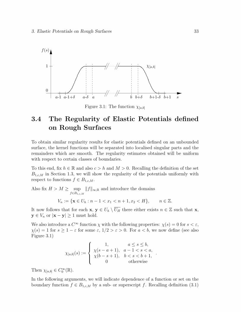
We also introduce a C∞ function χ with the following properties: χ(s) = 0 for s < ε,χ(s) = 1 for s ≥ 1− ε for some ε, 1/2 > ε > 0. For a < b, we now define (see alsoFigure 3.1)
χ[a,b](s) :=
1, a ≤ s ≤ b,
χ(s− a+ 1), a− 1 < s < a,χ(b− s+ 1), b < s < b+ 1,
0 otherwise
.
Then χ[a,b] ∈ C∞0 (R).
In the following arguments, we will indicate dependence of a function or set on theboundary function f ∈ B1,c,M by a sub- or superscript f . Recalling definition (3.1)
34 The Scattering of Elastic Waves by Rough Surfaces
of the elastic single layer potential on a rough surface, we define for f ∈ B1,c,M andφ ∈ [BC(Sf )]
2
vf1,n(x) :=
∫Sf
(ΓD,h(x,y)− χ[n−1,n+1](y1) Γ(x,y)
)φ(y) ds(y), x ∈ Vn \ Sf ,
and
vf2,n(x) :=
∫Sf
Γ(x,y)χ[n−1,n+1](y1)φ(y) ds(y), x ∈ Vn \ Sf .
On Vn \ Sf there obviously holds vf = vf1,n + vf2,n. We now analyse the regularityof these two vector fields.
Lemma 3.9 For f ∈ B1,c,M and α ∈ (0, 1), there holds vf1,n ∈ C0,α(Vn) and
‖vf1,n‖0,α;Vn ≤ C‖φ‖∞;Sf ,
where the constant C only depends on α, c, M , h and H.
Proof: For x ∈ Vn, y ∈ Sf , set
Kjk(x,y) := ΓD,h,jk(x,y)− χ[n−1,n+1](y1) Γjk(x,y), j, k = 1, 2.
From Theorems 2.10 and 2.13 as well as Theorem 2.16 we know Kjk is continuouslydifferentiable in Vn × Sf and that there exists a function κ ∈ L1(R) ∩ BC(R),dependent only on c, M , h and H such that
|Kjk(x,y)||gradxKjk(x,y)|
≤ κ(x1 − y1), x ∈ Vn,y ∈ Sf . (3.7)
Thus, we immediately obtain, for x ∈ Vn,
|vf1,n(x)| ≤ 4 (1 +M) ‖κ‖L1(R) ‖φ‖∞;Sf , x ∈ Vn. (3.8)
Now, for some ε > 0, set
Sx,ε := y ∈ Sf : |x1 − y1| < ε, x ∈ Vn.
Then, letting x, x′ ∈ Vn and assuming |x− x′| < ε, from (3.7) and the Mean ValueTheorem it follows that∣∣∣∣∣
∫Sx,2ε
(K(x,y)−K(x′,y))φ(y) ds(y)
∣∣∣∣∣≤ 16 (1 +M) ‖κ‖∞;R ε
2−α ‖φ‖∞;Sf |x− x′|α. (3.9)
3. Elastic Potentials on Rough Surfaces 35
On the other hand, we also have the estimate∣∣∣∣∣∫Sf\Sx,2ε
(K(x,y)−K(x′,y))φ(y) ds(y)
∣∣∣∣∣≤ 4 (1 +M) ‖κ‖L1(R) ε
1−α ‖φ‖∞;Sf |x− x′|α. (3.10)
Combining (3.8)–(3.10) yields the assertion for |x−x′| < ε. In the case |x−x′| > ε,from (3.8) we trivially obtain
|vf1,n(x)− vf1,n(x′)| ≤ 8 (1 +M) ε−α ‖κ‖L1(R) ‖φ‖∞;Sf |x− x′|α.
Lemma 3.10 For f ∈ B1,c,M , α ∈ (0, 1), there holds vf2,n ∈ C0,α(Vn) and
‖vf2,n‖0,α;Vn ≤ C‖φ‖∞;Sf ,
where the constant C only depends on α, c, M , h and H.
Proof: We define domains Dfn, f ∈ B1,c,M , in a manner very similar to the con-
struction described in Chapter 2, just before Theorem 2.7. Choosing ρ > 0, wedefine
χn(s) :=
χ(s− n+ 3), s < n− 2,
1, n− 2 ≤ s ≤ n+ 2,χ(n+ 3− s), n+ 2 < s,
where χ is the same cut-off function used earlier in this section, and set
f(s) := χn(s) f(s) + (1− χn(s)) (M + ρ).
A closed C1,1 boundary curve ∂Dfn will now be constructed as indicated below and
illustrated in Figure 3.2.
• between the points (n− 3, f(n− 3))> and (n+ 3, f(n+ 3))>, ∂Dfn is identical
to Sf := x ∈ R2 : x2 = f(x1),
• outside this section, ∂Dfn is continued by two half circles with radius ρ,
• ∂Dfn is closed by a straight line connecting the two half circles.
The domain Dfn is thus a bounded, simply connected domain of class C1,1. Moreover,
there are constants κ0, δ and M only dependent on c, M and ρ such that Dfn ⊂
D1,κ0,δ,Mfor all n ∈ Z and all f ∈ B1,c,M . Also, between (n − 2, f(n − 2)) and
(n+ 2, f(n+ 2)), ∂Dfn is identical to Sf .
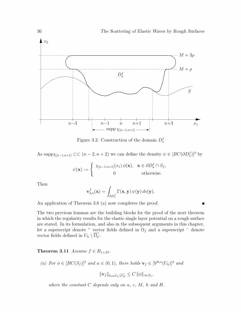
36 The Scattering of Elastic Waves by Rough Surfaces
n−3 n−1 n n+1 n+3suppχ[n−1,n+1]
Dfn
x1
x2
S
M + ρ
M + 3ρ
Figure 3.2: Construction of the domain Dfn
As suppχ[n−1,n+1] ⊂⊂ (n− 2, n+ 2) we can define the density ψ ∈ [BC(∂Dfn)]2 by
ψ(x) :=
χ[n−1,n+1](x1)φ(x), x ∈ ∂Df
n ∩ Sf ,0 otherwise.
Then
vf2,n(x) =
∫∂Dfn
Γ(x,y)ψ(y) ds(y).
An application of Theorem 3.6 (a) now completes the proof.
The two previous lemmas are the building blocks for the proof of the next theoremin which the regularity results for the elastic single layer potential on a rough surfaceare stated. In its formulation, and also in the subsequent arguments in this chapter,let a superscript denote + vector fields defined in Ωf and a superscript − denotevector fields defined in Uh \ Ωf .
Theorem 3.11 Assume f ∈ B1,c,M .
(a) For φ ∈ [BC(Sf )]2 and α ∈ (0, 1), there holds vf ∈ [V0,α(Uh)]
2 and
‖vf‖0,α;Uh\UH ≤ C ‖φ‖∞;Sf ,
where the constant C depends only on α, c, M , h and H.
3. Elastic Potentials on Rough Surfaces 37
(b) For φ ∈ [C0,α(Sf )]2, α ∈ (0, 1), the first order derivatives of v±f in Ωf and
in Uh \Ωf have C0,α-extensions to Ωf and Uh \Ωf respectively. Furthermore,there holds
‖v−f ‖1,α;Uh\Ωf , ‖v+f ‖1,α;Ωf\UH ≤ C ‖φ‖0,α;Sf ,
where the constant C depends only on α, c, M , h and H. For µ = µ (µ +λ)/(3µ+ λ) and λ = (2µ+ λ)(µ+ λ)/(3µ+ λ), there holds
Pv±f (x) = ∓1
2φ(x) +
∫Sf
Π(1)D,h(x,y)φ(y) ds(y), x ∈ Sf ,
where the integral exists as an improper integral.
(c) For φ ∈ [BC(Sf )]2 and α ∈ (0, 1), there holds∫
Sf
ΓD,h(·,y)φ(y) ds(y) ∈ [C0,α(Sf )]2,
where the integral exists as an improper integral. Furthermore,∥∥∥∥∥∫Sf
ΓD,h(·,y)φ(y) ds(y)
∥∥∥∥∥0,α;Sf
≤ C ‖φ‖∞;Sf ,
where the constant C depends only on α, c, M and h.
Proof: We immediately conclude from Lemmas 3.9 and 3.10 that vf ∈ C(Uh) andthat
‖vf‖∞;Uh\UH ≤ C‖φ‖∞;Sf (3.11)
where the constant C only depends on α, c, M , h and H. For x, y ∈ Uh \UH , thereeither exists n ∈ Z with x, y ∈ Vn or |x − y| ≥ 1. In the second case, we triviallyobtain from (3.11) that
|vf (x)− vf (y)| ≤ C‖φ‖∞;Sf |x− y|α.
In the first case, however, the same estimate follows from Lemmas 3.9 and 3.10.This concludes the proof of part (a).
As the kernel function in the definition of vf1,n is infinitely smooth, we can exchangethe order of integration and differentiation. Thus, in a way directly analogous tothe proof of Lemma 3.9 we obtain the same estimate for any first derivative of vf1,n.To see (b), we now proceed as in the proof of Lemma 3.10, only applying Theorem3.6 (b), and use the same arguments as for part (a).
Part (c) is an immediate consequence of part (a).
The same arguments as for Theorem 3.11 can be applied to prove regularity for thedouble-layer potential. We only have to employ Theorem 3.7 to obtain the followingtheorem.
38 The Scattering of Elastic Waves by Rough Surfaces
Theorem 3.12 Assume f ∈ B1,c,M .
(a) For φ ∈ [BC(Sf )]2, µ = µ (µ+λ)/(3µ+λ) and λ = (2µ+λ)(µ+λ)/(3µ+λ),
the double layer potential w±f in Ωf and in Uh \Ωf has continuous extensions
to Ωf and Uh \ Ωf respectively. Furthermore, there holds
‖w−f ‖∞;Uh\Ωf , ‖w+f ‖∞;Ωf
≤ C‖φ‖∞;Sf ,
where the constant C depends only on c, M , h and H, and
w±f (x) = ±1
2φ(x) +
∫Sf
Π(2)D,h(x,y)φ(y) ds(y), x ∈ Sf ,
where the integral exists as an improper integral.
(b) For φ ∈ [BC(Sf )]2, µ = µ (µ+λ)/(3µ+λ), λ = (2µ+λ)(µ+λ)/(3µ+λ) and
α ∈ (0, 1), there holds∫Sf
Π(j)D,h(·,y)φ(y) ds(y) ∈ [C0,α(Sf )]
2, j = 1, 2,
where the integral exists as an improper integral. Furthermore,∥∥∥∥∥∫Sf
Π(j)D,h(·,y)φ(y) ds(y)
∥∥∥∥∥0,α;Sf
≤ C ‖φ‖∞;S, j = 1, 2,
where the constant C depends only on α, c, M and h.
For certain arguments, it will also be necessary to study the elastic layer potentialsin the Sobolev space [H1
loc(Uh)]2. Making use of Remark 3.8 and using similar
arguments as in Lemmas 3.9 and 3.10, we obtain the following result:
Remark 3.13 Assume µ = µ (µ + λ)/(3µ + λ) and λ = (2µ + λ)(µ + λ)/(3µ + λ)
and φ ∈ [H1/2loc (S)]2. Then there holds v, w ∈ [H1
loc(Uh \ S)]2.
Chapter 4
Radiation Conditions andUniqueness
In this chapter, the rough surface scattering problem will be formulated mathemati-cally as a boundary value problem in the domain Ω. To ensure well-posedness of thisboundary value problem, a radiation condition has to be included in the formula-tion. We will thus begin by investigating some of the radiation conditions that havebeen used in elastic wave scattering problems. We then proceed to define a newradiation condition, termed the upward propagating radiation condition (UPRC)and analyse its properties, in particular how it generalises some of the more conven-tional conditions. We will then present the formulation of the scattering problem asa boundary value problem and, eventually, prove that this problem admits at mostone solution.
4.1 Radiation Conditions for Elastic Waves
From the perspective of physics, it is clear that the scattered field ought to bemade up of waves travelling along or away from the scattering obstacle. Whenformulating the problem as a boundary value problem, uniqueness of solution canonly be ensured if a mathematical characterisation of such fields is included in theformulation. Such a characterisation is termed a radiation condition.
Probably the best known radiation condition in scattering theory was that intro-duced by A. Sommerfeld in his Habilitation thesis [44] in 1896. A modern pre-sentation of this condition and its role for scattering problems involving boundedobstacles is given by Colton/Kress [23]. The formulation of Sommerfeld’s radi-ation condition for the elastic wave case is due to Kupradze [35], and a modernversion of this formulation is given here:
40 The Scattering of Elastic Waves by Rough Surfaces
Definition 4.1 Let D ⊂ R2 be a bounded domain. A solution u ∈ [C2(R2 \ D)]2
to the Navier equation in the exterior of D is said to satisfy Kupradze’s radiationcondition if
∂up∂r− ikpup = o(r−1/2) and
∂us∂r− iksus = o(r−1/2) (4.1)
uniformly in x/r as r := |x| → ∞.
In the case of scattering problems involving an effectively unbounded scatterer, itis not clear that (4.1) necessarily implies a specific decay rate for u(x) as |x| → ∞.Thus, for scattering problems of this type, we introduce the following notion of aradiating wave:
Definition 4.2 Let H ∈ R. A solution u ∈ [C2(UH)]2 to the Navier equation issaid to be radiating if
up = O(r−1/2),∂up∂r− ikpup = o(r−1/2)
and
us = O(r−1/2),∂us∂r− iksus = o(r−1/2)
uniformly in x/r for x ∈ UH as r := |x| → ∞.
Remark 4.3 A vector field satisfying Kupradze’s radiation condition in the senseof Definition 4.1 for some D ⊂ R2 is also radiating in the sense of Definition 4.2for any H such that D ∩ UH = ∅ (see, e.g., formula (3.63) in [23]).
As is to be expected, Γ also satisfies Kupradze’s radiation condition:
Theorem 4.4 The columns of the matrix functions Γ(·,y) and Π(2)(·,y) as well asthe rows of Γ(x, ·) and Π(1)(x, ·), x, y ∈ R2, satisfy Kupradze’s radiation condition.
Proof: For Γ, the assertion is proved as in [35] for the three dimensional case.For Π(1), Π(2), it can be seen by an application of Lemma 2.5 together with thecorresponding result for Γ.
In Section 2.4 when deriving the matrix of fundamental solutions ΓD,h, it was for-mulated as a requirement that the columns of the matrix function U represent wavefields propagating away from Th. We will now make this statement mathematicallyprecise, by showing they represent radiating solutions to the Navier equation:
4. Radiation Conditions and Uniqueness 41
Theorem 4.5 For x, y ∈ Uh and H > maxx2, y2, the columns of the matrixfunction ΓD,h(·,y) and the rows of the matrix function ΓD,h(x, ·) are radiating solu-tions to the Navier equation in UH .
Proof: As Γ is symmetric, the assertion for the first two terms in (2.22) is provedin Theorem 4.4 together with Remark 4.3. Thus, it suffices to show the assertionfor U.
Observe that the terms in (2.27) involving Mp represent the longitudinal and theterms involving Ms the transversal part of U; these will be denoted by U(p) andU(s), respectively. For fixed y, an entry U
(p)jk (·,y), j, k = 1, 2, satisfies the scalar
Helmholtz equation
∆z U(p)jk (z,y) + k2
p U(p)jk (z,y) = 0, z ∈ Uh,
and the boundary condition
U(p)jk (z,y) = g(z) := −Γjk(z,y) + Γjk(z,y
′h)−U
(s)jk (z,y), z ∈ Th.
From (2.27) we see, using arguments presented in [11], that U(p)jk satisfies the upward
propagating radiation condition of [11, 19], given here as Definition 4.8 and, moreprecisely, that
U(p)jk (z,y) = 2
∫Th
∂Φ
∂z2
(z, z) g(z) ds(z), z ∈ Uh,
where Φ(z, z) = i/4H(1)0 (kp|z − z|). Reviewing the proof of Theorem 2.13, we see
that g(z) = O(|z1|−3/2) as |z1| → ∞. We can thus use the argument presentedin [14, Section 5] to conclude
|U(p)jk (z,y)| ≤ C(1 + z2 − h)(1 + r)−3/2
and∂U
(p)jk
∂r(z,y)− ikpU(p)jk(z,y) = o(r−1/2),
where the derivative can be taken with respect to either z or y. The same argumentcan be applied to U(s)(·,y) and the proof is now completed by recalling Lemma2.15.
Corollary 4.6 For x, y ∈ Uh, H > maxx2, y2, the columns of Π(2)D,h(·,y) and the
rows of Π(1)D,h(x, ·) are radiating solutions to the Navier equation in UH .
42 The Scattering of Elastic Waves by Rough Surfaces
Proof: A direct consequence of the previous theorem by application of Lemma 2.5.
Much attention has also been paid to the special case of scattering by a periodicsurface, i.e. a diffraction grating. In this case, one usually imposes a radiationcondition using the Rayleigh expansion [5,27,36,37].
Definition 4.7 Assume f to be 2π-periodic. Then u ∈ BC(Ω) is said to satisfythe Rayleigh expansion radiation condition (RERC) if, for x2 > max f it has anexpansion of the form
u(x) =∑n∈Z
up,n
(αnβn
)ei(αnx1+βnx2) + us,n
(γn−αn
)ei(αnx1+γnx2)
,
where α ∈ R, α 6= 0, up,n, us,n ∈ C (n ∈ Z), αn := α + n,
βn :=
√k2p − α2
n, α2n ≤ k2
p
i√α2n − k2
p, α2n > k2
p
, γn :=
√k2s − α2
n, α2n ≤ k2
s
i√α2n − k2
s , α2n > k2
s
.
A field u satisfying the RERC is quasi-periodic with phase-shift α in Umax f andthus also, by analytic continuation, in Ω, that is, for all x = (x1, x2)> ∈ Ω,
u(x1 + 2π, x2) = eiα2π u(x1, x2).
As a periodic surface is a special case of a rough surface, the problem of scatteringby a diffraction grating can be seen as a special case of the problem of scattering bya rough surface. The radiation condition that will be introduced subsequently forscattering problems involving a rough surface will thus have to be satisfied by vectorfields satisfing the RERC as well as by radiating fields in the sense of Definition 4.2.It will be shown that this is indeed the case.
4.2 A New Radiation Condition for Scattering by
Rough Surfaces
We will start this section with a brief review of some results for the scalar case. Inthis case, the governing equation is the Helmholtz equation,
∆u+ k2 u = 0.
4. Radiation Conditions and Uniqueness 43
Its free field Green’s function is
Φ(x,y) :=i
4H
(1)0 (k |x− y|).
There has been considerable progress on such scalar wave scattering problems in-volving rough surfaces and inhomogeneous layers [11,15,19–21,48]. The foundationof much of these results is a new radiation condition, termed the upward propagatingradiation condition:
Definition 4.8 A solution u : G→ C to the Helmholtz equation in G ⊂ R2 is saidto satisfy the upwards propagating radiation condition (UPRC), if, for some H ∈ Rand φ ∈ L∞(TH), UH ⊂ G and
u(x) = 2
∫TH
∂Φ
∂y2
(x,y)φ(y) ds(y), x ∈ UH .
For the elastic wave case, a similar approach will be adopted. For the definition ofa UPRC, we will employ the matrix of fundamental solutions ΓD,h:
Definition 4.9 A solution u : G → C2 to the Navier equation (2.4) in G ⊂ R2
is said to satisfy the upward propagating radiation condition (UPRC), if, for someH ∈ R and φ ∈ [L∞(TH)]2, UH ⊂ G and
u(x) =
∫TH
Π(2)D,H(x,y)φ(y) ds(y), x ∈ UH . (4.2)
Remark 4.10 Note that from Theorem 2.16 (a) it follows that for arbitrary φ ∈[L∞(Th)]
2 the integral in (4.2) exists as an improper integral.
Remark 4.11 Apparently the definition of the upward propagating radiation con-dition depends on the choice of the parameters λ and µ in the definition of thegeneralised stresses. However, Theorem 4.12 below shows that the definition and thedensity φ itself are in fact independent of these numbers.
The following theorem characterises the UPRC further and also establishes, throughthe equivalence of (a) and (c), that it is satisfied by any radiating solution (c.f. thecharactarisation of the scalar UPRC in [19, Theorem 2.9]):
Theorem 4.12 Given a ∈ R and u : Ua → C2, the following statements are equiv-
alent:
44 The Scattering of Elastic Waves by Rough Surfaces
(a) u ∈ [C2(Ua)]2, u ∈ [L∞(Ua \ UH)]2 for all H > a, ∆∗ u + ω2u = 0 in Ua, and
u satisfies the UPRC in Ua.
(b) u ∈ [C2(Ua)]2, u ∈ [L∞(Ua \ UH)]2 for all H > a, ∆∗ u + ω2u = 0 in Ua, and
for some H > a and φ1, φ2 ∈ L∞(TH),
u(x) = 2 grad
∫TH
∂Φp
∂y2
(x,y)φ1(y) ds(y) + 2 grad⊥∫TH
∂Φs
∂y2
(x,y)φ2(y) ds(y)
for all x ∈ UH where Φp and Φs denote the fundamental solutions for theHelmholtz equation with k replaced by kp and ks, respectively.
(c) u ∈ [L∞(Ua \ UH)]2 for all H > a and there exists a sequence (un) of radiatingsolutions such that un(x)→ u(x) uniformly on compact subsets of Ua and
supx∈UH\Uh′ ,n∈N
|un(x)| <∞ (4.3)
for all H, h′ ∈ R satisfying h′ > H > a.
(d) u satisfies (4.2) for H = a and some φ ∈ [L∞(Ta)]2.
(e) u ∈ [L∞(Ua \ UH)]2 for some H > a and u satisfies (4.2) for each H > a withφ = u|TH .
(f) u ∈ [C2(Ua)]2, u ∈ [L∞(Ua \ UH)]2 for all H > a, ∆∗ u + ω2u = 0 in Ua, and
for every H > a and radiating solution in Ua, w, such that the restrictions ofw and Pw to TH are in [L1(TH)]
2, there holds∫
TH
(u ·Pw −w ·Pu) ds = 0. (4.4)
Proof: (a) ⇒ (b): With H chosen so that (4.2) holds, we introduce the functions
Ψp,k(x,y) := − 1k2p
divx Π(2)D,H,·k(x,y)
Ψs,k(x,y) := − 1k2s
div⊥x Π(2)D,H,·k(x,y)
k = 1, 2,
and rewrite u(x) for x ∈ UH as
u(x) = up(x) + us(x)
= grad
∫TH
2∑k=1
Ψp,k(x,y)φk(y) ds(y)
+ grad⊥∫TH
2∑k=1
Ψs,k(x,y)φk(y) ds(y). (4.5)
4. Radiation Conditions and Uniqueness 45
Limiting our attention to the first integral for the moment, we define
vN(x) =
∫TH(N)
2∑k=1
Ψp,k(x,y)φk(y) ds(y),
v(x) =
∫TH
2∑k=1
Ψp,k(x,y)φk(y) ds(y).
For H ′ > H, the vector fields vN are solutions to the Helmholtz equation ∆ vN +k2pvN = 0 in UH′ . By Corollary 4.6 and one applications of Lemma 2.5 we see that
they are furthermore radiating in UH′ . By Theorem 2.13 together with Lemma 2.5,there also holds vN(x)→ v(x) uniformly on compact subsets of UH′ . For h′ > H ′,by Remark 2.17, we finally see that
supx∈UH′\Uh′ ,n∈N
|vN(x)| <∞.
So by Theorem 2.1 in [19], v satisfies the UPRC for the Helmholtz equation (seeDefinition 4.8), which is the assertion. The argument for the second integral in (4.5)is identical.
(b) ⇒ (c): Set Ψ1 := −1/k2p div u and Ψ2 := −1/k2
s div⊥ u. Then (b) implies, thatfor all x ∈ UH there holds
Ψ1(x) = 2
∫TH
∂Φp
∂y2
(x,y)φ1(y) ds(y),
Ψ2(x) = 2
∫TH
∂Φs
∂y2
(x,y)φ2(y) ds(y).
From the equivalence of (i) and (ii) in Theorem 2.9 in [19], it follows that there exist
sequences (Ψ(n)j ) (j = 1, 2) of radiating solutions to the Helmholtz equation with
k = kp and k = ks respectively such that Ψ(n)j (x) → Ψj(x) uniformly on compact
subsets of Ua andsup
x∈Ua\Uh,n∈N,j=1,2
|Ψ(n)j (x)| <∞
for all h > a. Setun(x) := grad Ψ
(n)1 (x) + grad⊥Ψ
(n)2 (x).
Lemma 2.5 then implies (4.3) and that un(x) converges to u(x) uniformly on com-pact subsets of Ua.
(c) ⇒ (f): Suppose H > a and set D := UH ∩ BR(0) for some R > H, whereBR(0) denotes the open ball with centre 0 and radius R. Further assume w to bea radiating solution in Ua, such that the restrictions of w and Pw to TH are in[L1(TH)]
2. Then ∫
∂D
un ·Pw −w ·Pun ds = 0
46 The Scattering of Elastic Waves by Rough Surfaces
follows by the third generalised Betti formula (2.10). Letting R→∞ and using thefact that w and un are radiating solutions to the Navier equation, we conclude∫
TH
un ·Pw −w ·Pun ds = 0.
Taking the limit as n→∞, recalling (4.3) and using Lemma 2.5, we see that (4.4)holds. The remaining assertion follows from Corollary 2.6.
(f) ⇒ (a),(e): It suffices to show that (4.2) holds for all H > a with φ = u|TH .
Given H > a and x ∈ UH , choose h′, A ∈ R with h′ > x2 > H and A > |x1|. SetB := y ∈ UH \ Uh′ : |y1| < A. Then, by Theorem 2.16 (e),
u(x) =
∫∂B
ΓD,H(x,y) Pu(y)− Π
(2)D,H(x,y) u(y)
ds(y).
Letting A→∞ and recalling u ∈ [L∞(Ua \Uh′)]2 as well as Theorems 2.10 and 4.5as well as Theorem 2.16 (a), we obtain that
u(x) =
∫Th′
ΓD,H(x,y) Pu(y)− Π
(2)D,H(x,y) u(y)
ds(y)
+
∫TH
Π(2)D,H(x,y) u(y) ds(y).
By applying (4.4) with w equal to each of the rows of ΓD,H(x, ·) in turn, the integralover Th′ is seen to vanish.
(e) ⇒ (d): Introducing, for α ∈ R, the mapping
ηα(z) := (z1, z2 + α)>,
we have from (e) that
u(x) =
∫Ta
Π(2)D,H(x, ηH−a(z)) u(ηH−a(z)) ds(z), x ∈ UH . (4.6)
As u ∈ [L∞(Ua \ UH) ∩ C(Ua)]2 for some H > a, the densities u(ηH−a(·)) are all
in some ball in [L∞(Ta)]2 for H close enough to a. Recalling that the unit ball in
[L∞(Ta)]2 is weak∗ sequentially compact, there thus exists a sequence (Hn) with
Hn → a and u(ηHn−a(·)) → φ ∈ [L∞(Ta)]2. Taking the limit as H → a, through
this sequence in (4.6) we now conclude that (4.2) holds for H = a with this φ.
(d) ⇒ (c): As (4.2) is satisfied with h = a, it follows from Theorem 2.16 (a) that
|u(x)| ≤ ‖φ‖∞ g(x2), x ∈ Ua, (4.7)
4. Radiation Conditions and Uniqueness 47
where g ∈ C(R). Setting
un(x) :=
∫Ta(n)
Π(2)D,a(x,y)φ(y) ds(y), x ∈ Ua,
u ∈ [L∞(Ua \ Uh)]2 for all h > a and (4.3) follow from (4.7). That un(x) convergesto u(x) uniformly on compact subsets of Ua and that un is radiating, is also easilyseen from Theorem 2.16 (a).
Remark 4.13 From Remark 2.14 in [19] and the equivalence of statements (a) and(b) in Theorem 4.12, it follows that any bounded solution to the Navier equation uin Ω that satisfies the UPRC in Ω and is quasi-periodic in Ω also satisfies the RERCof Definition 4.7. Conversely, applying the same results, a bounded, quasi-periodicsolution to the Navier equation in Ω, satisfying the RERC, also satisfies the UPRC.
It remains to be shown that the elastic single- and double-layer potentials v definedby (3.1) and w defined by (3.2) satisfy the UPRC. To this end, assume f ∈ C1,1(R),φ ∈ [BC(S)]2 and introduce the vector fields vN and wN , N ∈ N, by
vN(x) :=
∫S(N)
ΓD,h(x,y)φ(y) ds(y),
wN(x) :=
∫S(N)
Π(2)D,h(x,y)φ(y) ds(y),
x ∈ Ω.
As SN is a bounded set, applications of Theorem 4.5 and Corollary 4.6 now yield thatvN and wN are radiating solutions to the Navier equation in the sense of Definition4.2 for any H > sup f . From Theorems 2.13 and 2.16 (a), the sequences (vN(x)) and(wN(x)) converge to v(x) and w(x), x ∈ Ω, respectively, and this convergence isuniform on compact subsets of Ua for any a > sup f . We can finally apply Theorem3.11 (a) and Theorem 3.12 (a) to see that (4.3) holds with a > sup f . Thus, theequivalence of (a) and (c) in Theorem 4.12 yields the following result:
Theorem 4.14 Assume f ∈ C1,1(R). Then, the elastic single-layer potential v andthe elastic double-layer potential w satisfy the UPRC.
4.3 Formulation as a Boundary Value Problem
and Uniqueness of Solution
Recall the formulation of the rough surface scattering problem from Section 1.1:
48 The Scattering of Elastic Waves by Rough Surfaces
Scattering Problem: Given an incident field uinc that is a solution to theNavier equation (2.4) in Ω, find the scattered field u such that uinc+u =0 on S.
We will now formulate this scattering problem as a boundary value problem. Infact, the assumptions can be formulated slightly more generally: we only requirethat uinc is a solution to the Navier equation in some neighborhood of S = ∂Ω andthat g := −uinc|S ∈ [BC(S) ∩H1/2
loc (S)]2.
Problem 4.15 Find a vector field u ∈ [C2(Ω) ∩ C(Ω) ∩H1loc(Ω)]2 that satisfies
1. the Navier equation ∆∗ u + ω2u = 0 in Ω,
2. the Dirichlet boundary condition u = g on S for some vector field g ∈[BC(S) ∩H1/2
loc (S)]2,
3. the vertical growth rate condition
supx∈Ω
xβ2 |u(x)| <∞ (4.8)
for some β ∈ R and
4. the UPRC in Ω.
Remark 4.16 A solution of Problem 4.15 satisfies statement (a) of Theorem 4.12with any a > sup f .
The remaining part of this chapter will be devoted to proving that Problem 4.15 hasat most one solution. The question of existence of solution will be postponed untilChapter 5. However, it is worth pointing out at this stage, that it is clear a priorithat Problem 4.15 is well posed in certain, non-trivial cases: From Remark 4.13 wesee that, in the case when f is periodic and the Dirichlet data g is quasi-periodic,Problem 4.15 reduces to the diffraction grating problem considered in [4, 5], if weassume additionally that the solution u is quasi-periodic. The diffraction gratingproblem was shown in [4, 5] to be uniquely solvable. Thus we know that Problem4.15 admits solutions, in the case when f is periodic and g quasi-periodic.
Let us also point out that, as we will now proceed to show that Problem 4.15 hasat most one solution in every case, we will in fact prove for the diffraction gratingproblem that the additional requirement that the solution be quasi-periodic can bedropped.
In all of what follows, let h denote a real number with h < inf f . The first step inthe uniqueness proof will be the following representation theorem:
4. Radiation Conditions and Uniqueness 49
Theorem 4.17 Let u be a solution to Problem 4.15 with g ≡ 0. Then u ∈ [C1(Ω)]2,its first derivatives are bounded in DH for any H > sup f and
u(x) = −∫S
ΓD,h(x,y) Pu(y) ds(y)
holds for all x ∈ Ω.
Proof: That u ∈ [C1(Ω)]2 and its first derivatives are bounded in DH , H > sup f ,is a consequence of Theorem 2.7. For x ∈ Ω, choose h′, A ∈ R and ε > 0 withh′ > maxx2, sup f and A > |x1|. Define DA
ε,h′ := x ∈ Dh′(A) : x2 > f(x1) + ε.Then, by Theorem 2.16 (e), there holds
u(x) =
∫∂DA
ε,h′
ΓD,h(x,y) Pu(y)− Π
(2)D,h(x,y) u(y)
ds(y).
By applying Theorem 2.7, we see that the growth rate condition (4.8) for u alsoholds for any first derivative of u. Letting A→∞ and recalling Theorems 2.13 and2.16 (a) then yields
u(x) =
∫Th′
ΓD,h(x,y) Pu(y)− Π
(2)D,h(x,y) u(y)
ds(y)
−∫Sε
ΓD,h(x,y) Pu(y)− Π
(2)D,h(x,y) u(y)
ds(y),
where Sε := x ∈ Ω : x2 = f(x1) + ε. Note here, that the normal n to Sε isassumed to be pointing upwards. The proof is now completed by recalling Remark4.16 and the equivalence of (a) and (f) in Theorem 4.12, by which the integral overTh′ vanishes, and letting ε→ 0.
Let us now introduce some functionals that will be of importance in the followingarguments. Let h′ > sup f , A > 0 and u ∈ C1(Ω). We define
I(h′, A)[u] :=
∫Th′ (A)
(2µ+ λ)
(∣∣∣∣∂u2
∂x2
∣∣∣∣2 − ∣∣∣∣∂u1
∂x1
∣∣∣∣2)
+µ
(∣∣∣∣∂u1
∂x2
∣∣∣∣2 − ∣∣∣∣∂u2
∂x1
∣∣∣∣2)
+ ω2|u|2 ds,
J1(h′, A)[u] := 2 Re
∫γ(h′,A)
∂u
∂x2
·Pu ds,
J2(h′, A)[u] := Im
∫γ(h′,A)
u ·Pu ds,
K(h′, A)[u] := Im
∫Th′ (A)
u ·Pu ds,
50 The Scattering of Elastic Waves by Rough Surfaces
where we recall the assumptions on the direction of the normal vectors in Section1.3. We will now investigate the properties of these functionals.
Lemma 4.18 Suppose u satisfies statement (b) in Theorem 4.12 with H > sup fand some densities φj ∈ L2(TH) ∩ L∞(TH) (j = 1, 2). Then, for all h′ > H, thereholds
I(h′,∞)[u] = 2ω2
∫ kp
−kp|φ1|2γ2
p dt+
∫ ks
−ks|φ2|2γ2
s dt
,
where φ1(t) := e−iγpH φ1(t), φ2(t) := e−iγsH φ2(t) and φj denotes the Fourier trans-form of φj(y1, y2) with respect to y1 (j = 1, 2), i.e.
φj(t) =
∫ ∞−∞
φj(y1, y2) eiy1t dy1.
Proof: Choose H > sup f so that the representation for u in UH according to state-ment (b) of Theorem 4.12 holds. Then the argument presented for the derivationof equation (29) in [11] yields
u(x) =i
2π
∫ ∞−∞
φ1(t)
(t
γp
)ei(tx1+γpx2) + φ2(t)
(γs−t
)ei(tx1+γsx2) dt, x ∈ UH .
By an application of Parseval’s Theorem we derive from this representation, for anyh′ > H, ∫
Th′
|u1|2ds =
∫ ∞−∞|tφ1 + γsφ2|2dt,∫
Th′
|u2|2ds =
∫ ∞−∞|γpφ1 − tφ2|2dt,∫
Th′
∣∣∣∣∂u1
∂x1
∣∣∣∣2 ds =
∫ ∞−∞|it2φ1 + itγsφ2|2dt,∫
Th′
∣∣∣∣∂u1
∂x2
∣∣∣∣2 ds =
∫ ∞−∞|itγpφ1 + iγ2
s φ2|2dt,∫Th′
∣∣∣∣∂u2
∂x1
∣∣∣∣2 ds =
∫ ∞−∞|itγpφ1 − it2φ2|2dt,∫
Th′
∣∣∣∣∂u2
∂x2
∣∣∣∣2 ds =
∫ ∞−∞|iγ2
p φ1 − itγsφ2|2dt.

4. Radiation Conditions and Uniqueness 51
From these formulae, the following three identities are easily obtained:∫Th′
|u1|2 + |u2|2
ds =
∫ ∞−∞|φ1|2 (t2 + |γp|2) + φ1 φ2 (tγs − tγp)
+φ1 φ2 (tγs − tγp) + |φ2|2 (|γs|2 + t2) dt,(4.9)∫Th′
∣∣∣∣∂u2
∂x2
∣∣∣∣2 +
∣∣∣∣∂u1
∂x1
∣∣∣∣2ds =
∫ ∞−∞|φ1|2 (γ4
p − t4) + φ1 φ2 (−tγ2pγs − t3γs)
+φ1 φ2 (−tγ2pγs − t3γs) dt, (4.10)∫
Th′
∣∣∣∣∂u1
∂x2
∣∣∣∣2 +
∣∣∣∣∂u2
∂x1
∣∣∣∣2ds =
∫ ∞−∞
φ1 φ2 (tγpγ2s + t3γp) + φ1 φ2 (tγpγ
2s − t3γp)
+|φ2|2 (γ4s − t4) dt. (4.11)
Combining (4.9)–(4.11) and observing k2p − t2 + |γp|2 = 0 for |t| > kp as well as
k2s − t2 + |γs|2 = 0 for |t| > ks now yields the assertion.
Lemma 4.19 Suppose all the assumptions of Lemma 4.18 are satisfied. Then, forall h′ > H, we have the identity
K(h′,∞)[u] = ω2
∫ kp
−kp|φ1|2γp dt+
∫ ks
−ks|φ2|2γs dt
.
Proof: Recalling the remarks at the beginning of the proof of Lemma 4.18 andadopting the same notation, we easily see that∫
Th′
u ·Pu ds =
∫ ∞−∞
|φ1|2(iµt2γp + iµt2γp + iλt2γp + i(2µ+ λ)γpγ
2p)
+ φ1φ2(iµtγpγs + iµtγpγs − iλt3 − i(2µ+ λ)tγ2p)
+ φ1φ2(iµtγ2s − iµt3 + iλtγpγs − i(2µ+ λ)tγpγs)
+ |φ2|(iµγ2sγs − iµt2γs − iλt2γs + i(2µ+ λ)t2γs)
dt.
(4.12)
Taking the imaginary part, straightforward calculations show that all the terms
involving φ1φ2 and its complex conjugate cancel. On the other hand,
Im
∫ ∞−∞|φ1|2(iµt2γp + iat2γp + ibt2γp + i(2µ+ λ)γpγ
2p) dt
52 The Scattering of Elastic Waves by Rough Surfaces
=1
2
∫ ∞−∞|φ1|2 (µt2γp + µt2γp + µt2γp + µt2γp
+λt2γp + λt2γp + (2µ+ λ)γpγ2p + (2µ+ λ)γ3
p dt
=1
2
∫ ∞−∞
(2µ+ λ) |φ1|2 (t2γp + γ3p + t2γp + γpγ
2p) dt
=
∫ kp
−kp(2µ+ λ)k2
pγp|φ1|2 dt
A similar calculation for the remaining term in the expression (4.12) now yields thelemma.
The following corollary to the previous two lemmas is of fundamental importance:
Corollary 4.20 Suppose all the assumptions of Lemma 4.18 are satisfied. Then,for all h′ > H, there holds
I(h′,∞)[u] ≤ 2ksK(h′,∞)[u].
Proof: The assertion follows from Lemmas 4.18 and 4.19 by noting kp ≥ γp on[−kp, kp], ks ≥ γs on [−ks, ks] and ks > kp.
Another, simpler relation involving these functionals which is much easier to proveis stated in the following lemma:
Lemma 4.21 Let u be a solution to Problem 4.15 with g ≡ 0. Further assumeh′ > max f and A > 0. Then
K(h′, A)[u] = −J2(h′, A)[u].
Proof: Apply the third generalised Betti formula (2.10) to u and u in Dh′(A).
Assume now that u is a solution to Problem 4.15 with g ≡ 0. As u and its tangentialderivatives vanish on S, Pu has the simple form
Pu = µ∂u
∂n+ (λ+ µ) n div u on S, (4.13)
and thus∫S(A)
∂u
∂x2
·Pu ds =
∫S(A)
µn2
∣∣∣∣∂u
∂n
∣∣∣∣2 + (λ+ µ)n2 |div u|2ds (4.14)
4. Radiation Conditions and Uniqueness 53
for any A > 0. In a similar fashion, we also show that
Eµ,λ(u,u) = µ
∣∣∣∣∂u
∂n
∣∣∣∣2 + (λ+ µ) |div u|2 on S. (4.15)
Combining (4.14) and (4.15), we conclude by an integration by parts that
0 ≤∫S(A)
µn2
∣∣∣∣∂u
∂n
∣∣∣∣2 + (λ+ µ)n2|div u|2ds
= 2 Re
∫S(A)
∂u
∂x2
·Pu ds−∫S(A)
n2 Eµ,λ(u,u)− n2 ω2|u|2 ds
= 2 Re
∫S(A)
∂u
∂x2
·Pu ds+ 2 Re
∫Dh′ (A)
Eµ,λ(∂u
∂x2
,u)− ω2 ∂u
∂x2
· u dx
−∫Th′ (A)
Eµ,λ(u,u)− ω2|u|2 ds (4.16)
On the other hand, for any h′ > sup f , by the first Betti formula (2.8) there alsoholds ∫
∂Dh′ (A)
∂u
∂x2
·Pu ds =
∫Dh′ (A)
Eµ,λ(∂u
∂x2
,u)− ω2 ∂u
∂x2
· u dx. (4.17)
It is also not difficult to see that
Re
∫Th′ (A)
2∂u
∂x2
·Pu + ω2|u|2 − Eµ,λ(u,u)
ds = I(h′, A)[u],
Combining this identity with (4.16) and (4.17), we conclude finally that
0 ≤∫S(A)
µn2
∣∣∣∣∂u
∂n
∣∣∣∣2 + (λ+ µ)n2|div u|2ds = I(h′, A)[u] + J1(h′, A)[u]. (4.18)
The rest of the derivation of the uniqueness result is now a rather straightforwardadaption of the method presented in [20] for the Helmholtz equation case. Let usintroduce the vector fields vA defined for A > 0 by
vA(x) := −∫S(A)
ΓD,h(x,y) Pu(y) ds(y).
Using the Cauchy-Schwarz inequality and Theorem 2.13, we find that vA|h′ ∈[L2(Th′) ∩ BC(Th′)]
2 for all h′ > sup f . As vA is a radiating solution to the Navierequation for every A ∈ R, it is seen to satisfy statement (c) of Theorem 4.12 andthus also statement (b) of that theorem. Thus, by Corollary 4.20,
I(h′,∞)[vA] ≤ 2ksK(h′,∞)[vA]. (4.19)
54 The Scattering of Elastic Waves by Rough Surfaces
Now set w(x1) := |Pu(x1, f(x1))| for x1 ∈ R. Then∫ A
−A|w(x1)|2 dx1 ≤
∫S(A)
|Pu|2 ds ≤ (1 + ‖f ′‖2∞;R)1/2
∫ A
−A|w(x1)|2 dx1 (4.20)
follows. Using Theorem 2.13 and Lemma 2.5 we obtain the estimates
|ΓD,h(x,y)|, | ∂∂xj
ΓD,h(x,y)| ≤ C(1 + |x1 − y1|)−3/2 (j = 1, 2)
for x ∈ Th′ , y ∈ S, where C is some positive constant depending only on h′ and h.This yields the estimates
|vA(x)|, |∂vA∂xj
(x)| ≤ CWA(x1)
|u(x)− vA(x)| ≤ C (W∞(x1)−WA(x1))
| ∂u∂xj
(x)− ∂vA∂xj
(x)| ≤ C (W∞(x1)−WA(x1))
(4.21)
for x ∈ Th′ , j = 1, 2, with certain generic constants C, where
WA(x1) :=
∫ A
−A(1 + |x1 − y1|)−3/2 w(y1) dy1, x1 ∈ R.
Recalling (4.13), we can estimate by (4.18)–(4.20) and Lemma 4.21∫ A
−A|w(x1)|2 dx1 ≤ C
∫S(A)
µn2
∣∣∣∣∂u
∂n
∣∣∣∣2 + (λ+ µ)n2|div u|2ds
≤ C|I(h′, A)[u]− I(h′, A)[vA]|
+|I(h′, A)[vA]− I(h′,∞)[vA]|
+2ks
[|K(h′,∞)[vA]−K(h′, A)[vA]|
+|K(h′, A)[vA]−K(h′, A)[u]|]
+|J1(h′, A)[u]|+ 2ks|J2(h′, A)[u]|.
From (4.21), there now follows, with some positive constant C,
|I(h′, A)[vA]− I(h′,∞)[vA|,|K(h′,∞)[vA]−K(h′, A)[vA]|
≤ C
∫R\[−A,A]
W 2A(x1) dx1
and
|I(h′, A)[u]− I(h′, A)[vA]|,|K(h′, A)[vA]−K(h′, A)[u]|
≤ C
∫ A
−A(W∞(x1)−WA(x1))W∞(x1) dx1,
4. Radiation Conditions and Uniqueness 55
so that we finally conclude, for some constant c > 0 and all A > 0,∫ A
−A|w(x1)|2 dx1 ≤ c
∫R\[−A,A]
W 2A(x1) dx1
+
∫ A
−A(W∞(x1)−WA(x1))W∞(x1) dx1
+|J1(h′, A)[u]|+ |J2(h′, A)[u]|. (4.22)
Since (4.22) holds and we also have from Theorem 2.7 that w ∈ L∞(R), we canapply Lemma A in [20] to obtain that w ∈ L2(R) and, noting (4.20), that for allA0 > 0,
(1 + ‖f ′‖2∞;R)−1/2
∫S
|Pu|2 ds ≤∫ ∞−∞|w(x1)|2 dx1
≤ c supA>A0
|J1(h′, A)[u]|+ |J2(h′, A)[u]|.(4.23)
For x ∈ Dh′ with |x1| > 0, we now deduce by Theorem 2.13, Theorem 4.17 and theCauchy-Schwarz inequality, that
|u(x)|2 ≤ 2
∫S\S(|x1|/2)
|ΓD,h(x,y) Pu(y)| ds(y)
2
+ 2
∫S(|x1|/2)
|ΓD,h(x,y) Pu(y)| ds(y)
2
≤ C1
∫S\S(|x1|/2)
|Pu|2 ds+ C2
(|x1|2
)−2
,
where
C1 = 16 supx∈Dh′
∫S
maxj,k=1,2
|ΓD,h,jk(x,y)|2 ds(y) <∞
by Remark 2.14 and
C2 = 32 ‖H‖2C([0,h′−h]2) (1 + ‖f ′‖∞;R)1/2 ‖Pu‖[L2(S)]2 .
Thus, u(x) → 0 as |x1| → ∞ (x ∈ Dh′), uniformly in x2. From Lemma 2.5and Theorem 2.7 it now follows that Jj(A)[u] → 0 as A → ∞ (j = 1, 2), andconsequently, by (4.23), that Pu = 0 on S. Recalling once more Theorem 4.17, weconclude u ≡ 0 in Ω.
We have thus shown the following central theorem:
Theorem 4.22 Let u and v be solutions of Problem 4.15 with the same Dirichletdata g. Then u ≡ v in Ω.

56 The Scattering of Elastic Waves by Rough Surfaces
Chapter 5
Existence of Solution
Existence of solution will be proved by the boundary integral equation method,a well-established method to prove existence of solution for scattering problems.As a first step, an equivalent integral equation formulation of Problem 4.15 willbe derived. However, as the integral operators in this equation are not compact,surjectivity cannot be deduced from injectivity by the Fredholm Alternative, aswould be the usual approach in scattering by bounded obstacles. A new theory ofsolvability of integral equations on unbounded domains will be presented that allowsthis deduction for problems of scattering by infinite rough surfaces. This theory isused to establish solvability in [BC(R)]2, first for the adjoint equation and then,through a duality argument, for the orginal equation. As a final result, it is shownhow it is possible to establish solvability in all [Lp(R)]2 spaces.
5.1 An Integral Equation Formulation
The first stepping stone in the existence proof will be an equivalent integral equationformulation of Problem 4.15. To derive this equation, we will seek a solution toProblem 4.15 in the form of a combined single- and double layer potential,
u(x) =
∫S
Π
(2)D,h(x,y)− iη ΓD,h(x,y)
ψ(y) ds(y), x ∈ Ω, (5.1)
where ψ ∈ [BC(S)∩H1/2loc (S)]2 and η is a complex number with Re (η) > 0. Through-
out, we assume µ = µ (µ+ λ)/(3µ+ λ) and λ = (2µ+ λ)(µ+ λ)/(3µ+ λ) and thatf ∈ C1,1(R).
From Theorem 3.1 we know that u is a solution to the Navier equation in Ω andin Uh \ Ω. Note also Remark 3.13 to see u ∈ [H1
loc(Ω)]2. Furthermore, it satisfies
58 The Scattering of Elastic Waves by Rough Surfaces
the UPRC by Theorem 4.14. A review of the derivation of Theorem 2.13 furtherreveals that the function H in this theorem satisfies H(x2, y2) = O(x2) as x2 →∞,uniformly for bounded y2. Therefore, the growth condition (4.8) can be seen to holdwith β = −1/2.
Thus, from the jump relations for elastic single- and double-layer potentials statedin Theorems 3.11 and 3.12 and the boundary condition, it follows that u is a solutionto the boundary value problem if ψ is a solution to the integral equation
1
2ψ(x) +
∫S
Π
(2)D,h(x,y)− iη ΓD,h(x,y)
ψ(y) ds(y) = −g(x), x ∈ S. (5.2)
It suffices to study the solvability of this integral equation in the space [BC(S)]2,as it follows from Theorems 3.11 (c) and 3.12 (b) that the integral operator maps
[BC(S)]2 into [H1/2loc (S)]2. Thus, for any right hand side g ∈ [BC(S) ∩ H1/2
loc (S)]2,the solution has to be an element of this space as well.
We now introduce the three integral operators Sf , Df and D′f by
Sf φ(s) := 2
∫ ∞−∞
ΓD,h((s, f(s)), (t, f(t))φ(t)√
1 + f ′(t)2 dt, (5.3)
Df φ(s) := 2
∫ ∞−∞
Π(2)D,h((s, f(s)), (t, f(t)))φ(t)
√1 + f ′(t)2 dt, (5.4)
D′f φ(s) := 2
∫ ∞−∞
Π(1)D,h((s, f(s)), (t, f(t)))φ(t)
√1 + f ′(t)2 dt, (5.5)
where s ∈ R and φ ∈ [L∞(R)]2. From Theorem 3.11 (c) and Theorem 3.12 (b),we know that each of these operators are bounded mappings of [BC(R)]2 into[C0,α(R)]2. Furthermore, setting φ(s) = ψ(s, f(s)), the integral equation (5.2) isequivalent to
(I + Df − iη Sf )φ(s) = −2 g(s, f(s)), s ∈ R. (5.6)
We explore the properties of these three integral operators more thoroughly in thefollowing lemmas:
Lemma 5.1 Let K denote any of the integral operators Sf , Df or D′f and K(s, t)
the corresponding matrix kernel, such that Kφ(s) =∫∞−∞K(s, t)φ(t) dt.
(a) There exists a function κ ∈ L1(R) such that
maxj,k=1,2
|Kjk(s, t)| ≤ κ(s− t) for almost all s, t ∈ R,
where κ = O(|s|−3/2) as |s| → ∞.
5. Existence of Solution 59
(b) The matrix kernel K of K satisfies the properties
sups∈R
∫ ∞−∞|Kjk(s, t)| dt <∞, j, k = 1, 2, (5.7)
and, for all s, s′ ∈ R,
lims′→s
∫ ∞−∞|Kjk(s, t)−Kjk(s
′, t)| dt = 0, j, k = 1, 2. (5.8)
(c) K is a bounded mapping from [L∞(R)]2 to [BC(R)]2.
(d) K is a bounded mapping from [Lp(R)]2 to [Lp(R)]2 for any p ∈ [1,∞).
Proof: For s, t ∈ R, let x = (s, f(s)), y = (t, f(t)). Then, by (2.14) and Theorems2.10 and 2.13, for ε > 0, j, k = 1, 2, there exists a constant C > 0 and H ∈ C(R2)such that
|ΓD,h,jk(x,y)| ≤
C (1 + log |x− y|), |s− t| ≤ ε,
H(f(s)−h,f(t)−h)
|s−t|3/2 , |s− t| > ε.
The same estimate is valid for the fundamental matrices Π(1)D,h and Π
(2)D,h by Theorem
2.16 and Remark 3.4. Thus (a) follows immediately.
Property (5.7) is a simple consequence of (a) while property (5.8) follows from thedominated convergence theorem. (5.7) and (5.8) together imply statement (c).
Statement (d) follows from (a) using Young’s Theorem.
Lemma 5.2 The operator Sf is self-adjoint and the operators Df and D′f areadjoint with respect to the non-degenerate duality < ·, · > defined on [Lp(R)]2 ×[Lq(R)]2, by
< φ, ψ > :=
∫ ∞−∞
φ(s) · ψ(s)√
1 + f ′(s)2 ds, (5.9)
where either 1 < p, q <∞ with 1/p+ 1/q = 1 or p = 1 and q =∞.
Proof: The assertion follows from Lemma 5.1 (d) as well as Lemma 2.15 andTheorem 2.16 (b).
As the operators Sf and Df are not compact on any suitable space, the FredholmAlternative is not available as a tool to deduce surjectivity of I + Df − iη Sf frominjectivity. We will nevertheless present a theory in the subsequent sections thatallows this deduction.
However, it is also not straightforward to show injectivity of I + Df − iη Sf . Wewill therefore start by considering the adjoint operator:
60 The Scattering of Elastic Waves by Rough Surfaces
Theorem 5.3 The operator I + D′f − iη Sf is injective on [L∞(R)]2.
Proof: Because of Lemma 5.1 (c), any vector density φ ∈ [L∞(R)]2 in the kernel ofI + D′f − iη Sf has to be in [BC(R)]2. It is therefore enough to show injectivity onthis space.
Assume φ ∈ [BC(R)]2 to be a solution of
(I + D′f − iη Sf )φ = 0, (5.10)
and define the single layer potential u by
u(x) :=
∫S
ΓD,h(x,y)φ(y1) ds(y) for x ∈ Uh \ S,
where h ∈ R with h < inf f . Let us introduce the notation u+ = u|Ω and u− =u|Uh\Ω. From (5.10) and the mapping properties of Sf and D′f it follows thatφ ∈ [C0,α(R)]2. Thus, from Theorem 3.11, we have that u− and u+ have continuousderivatives up to S and, moreover, that
‖u−‖1,α;Uh\Ω ≤ C ‖φ‖0,α;S, (5.11)
Pu− − iη u− = 0 on S, (5.12)
φ = Pu− −Pu+. (5.13)
Also, by the definition of ΓD,h, there holds u− = 0 on Th. Thus, by an applicationof the first generalised Betti formula,
Re(η)
∫S(A)
|u−|2 ds = − 1
2i
∫S(A)
u− ·Pu− − u− ·Pu−
ds
=1
2i
∫R(A)
u− ·Pu− − u− ·Pu−
ds, (5.14)
where R(A) := x ∈ Uh \ Ω : |x1| = A. Note that the right hand side of thisequation is bounded by (5.11), so u− ∈ [L2(S)]2 follows by taking the limit asA→∞. Consequently, (5.12) yields Pu− ∈ [L2(S)]2 as well.
It is not difficult to see that
u−(x) =
∫S
ΓD,h(x,y) Pu−(y)− Π
(2)D,h(x,y) u−(y)
ds(y)
holds for all x ∈ Uh\Ω. Thus, by an argument very similar to that in the uniquenessproof for the Dirichlet problem, it follows that |u−(x)| → 0 as |x1| → ∞. Applyingthis in (5.14) and taking the limit for A→∞, then yields u− = 0 on S.
From the continuity of the elastic single-layer potential in Uh, there follows u+ = 0on S and thus, by the uniqueness theorem for the Dirichlet problem, Pu+ = 0 onS. Also, (5.12) implies Pu− = 0 on S. Thus, by (5.13), we conclude φ ≡ 0.
5. Existence of Solution 61
5.2 Solvability results for a class of operator equa-
tions
To deduce the surjectivity of the integral operators from their injectivity, we will nowpresent a solvability theory developed by Chandler-Wilde, Zhang and Ross
[10,17,22] which generalises the collectively compact operator theory of Anselone
[1]. The operator equation approach presented here is that used in [16].
Let X denote a Frechet space with a countable family of semi-norms | · |n thatgenerates the topology onX. This topology shall be labelled τ . We define a subspaceY of X by
Y := φ ∈ X : ‖φ‖∞ := supn∈N|φ|n <∞.
We note that ‖ · ‖∞ is a norm on Y and that Y becomes a Banach space under thisnorm. The corresponding topology shall be termed the norm topology.
Example 5.4 In the context of the application of this theory to the integral equa-tion (5.6), we will use X = [C(R)]2 with
|φ|n = sup|t|≤n|φ(t)|,
so that Y = [BC(R)]2.
On the space Y we now define a further topology as follows. Let S0 denote thespace of real sequences converging to 0,
S0 := (an) : an ∈ R, n ∈ N, limn→∞
an = 0.
For each a ∈ S0, we define a seminorm | · |a on Y by
|φ|a := supn∈N|an φ|n.
Clearly, the family of seminorms | · |a : a ∈ S0 is separating. Thus it induces alocally convex topology on Y , which we will call the σ-topology.
Remark 5.5 The σ-topology is an abstraction of the strict topology introduced byBuck in [9].
Remark 5.6 For (φn) ⊂ Y , we write φn −→ φ if ‖φn − φ‖∞ → 0 as n→∞, andφn
σ−→ φ if (φn) converges in the σ-topology. It is easy to see that
φnσ−→ φ =⇒ ‖φ‖∞ ≤ sup
n∈N‖φn‖∞. (5.15)
62 The Scattering of Elastic Waves by Rough Surfaces
The following theorem explores the properties of the σ-topology and its relation tothe other two topologies.
Theorem 5.7
(a) The bounded sets in Y in the σ-topology and in the norm topology are thesame.
(b) Y is complete in the σ-topology.
(c) A sequence (φn) ⊂ Y is convergent in the σ-topology if and only if it is con-vergent in the τ -topology and (φn) is bounded in the norm topology.
(d) The σ-topology is either identical to the norm topology or it is not metrizable.
(e) If K : Y → Y is a linear operator and K is bounded in the σ-topology then itis also continuous in the norm topology.
Proof: Obviously any bounded set in the norm topology is bounded in the σ-topology. Assume B ⊂ Y to be bounded in the σ-topology but not in the normtopology. Then, there exists a sequence (φn) ⊂ B and a sequence (an) ∈ S0 suchthat |φ|n ≥ a−2
n . But then,
|an φ|n ≥1
|an|−→ ∞, n→∞,
which is a contradiction. Thus (a) follows.
Next, we prove (c). Let (φn) ⊂ Y be convergent with limit φ ∈ Y in the σ-topology.Then clearly, (φn) is bounded in the σ-topology and thus also bounded in the normtopology by (a). If, for j ∈ N, we choose a ∈ S0 such that aj = 1, then there holds
|ψ|j ≤ |ψ|a, ψ ∈ Y. (5.16)
Thus φn → φ in the τ -topology as well. Conversely, assume (φn) ⊂ Y to bebounded in the norm topology and convergent to φ ∈ X in the τ -topology. LetM := supn∈N ‖φn‖∞. Then, for every k ∈ N there exists n(k) ∈ N such that|φ− φn(k)|k ≤M . Thus,
|φ|k ≤ |φ− φn(k)|k + |φn(k)|k ≤ 2M,
and consequently φ ∈ Y . Therefore, now φnσ−→ φ.
To prove (b), assume (φn) ⊂ Y to be a Cauchy sequence in the σ-topology. Then,by (a), it is bounded in the norm topology and by (5.16), (φn) is also a Cauchy
5. Existence of Solution 63
sequence in X with respect to the τ -topology and thus convergent. Therefore, (c)now implies that (φn) is convergent in the σ-topology.
To prove (d), assume that the σ-topology is metrizable. Then, by Baire’s Theorem[43, Theorem 2.2], (Y ,σ) is of second category in itself and thus, by the OpenMapping Theorem [43, Theorem 2.11], the mapping id : (Y, ‖ ·‖∞)→ (Y, σ) is open.But the σ-topology is weaker than the norm topology so both must be identical.
By (a), an operator K bounded in the σ-topology is also bounded in the normtopology. As boundedness is equivalent to continuity on normed spaces, (e) follows.
Definition 5.8 A set B ⊂ Y is said to be relatively sequentially compact in theσ-topology if any sequence in B has a subsequence that is convergent in the σ-topology. A linear operator K is said to be relatively sequentially compact withrespect to (w.r.t.) the σ-topology if for any bounded set B ⊂ Y , K(B) is relativelysequentially compact in the σ-topology. A family K of linear operators on Y is saidto be collectively sequentially compact w.r.t. the σ-topology if for any bounded setB ⊂ Y the set
⋃K∈KK(B) is relatively sequentially compact in the σ-topology.
In some of the subsequent arguments we will also make use of the following notion:
Definition 5.9 An operator L : Y → Y is said to be σ-norm-continuous, if it iscontinuous as an operator from (Y, σ) to (Y, ‖ · ‖).
We also denote, as is usual, the set of Fredholm operators on a given topologicalvector space V by Φ(V ) .
The following Lemma, in a less general form, is due to Haseloh [32,33] and in theproof we follow the original argument.
Lemma 5.10 Let K, L be sequentially compact w.r.t the σ-topology and assumeadditionally that L is σ-norm-continuous.
(a) LK is compact.
(b) I − L ∈ Φ(Y ) with ind (I − L) = 0.
(c) I −K − L ∈ Φ(Y ) if and only if I −K ∈ Φ(Y ). If one of these statementshold then the index of both operators is the same.
64 The Scattering of Elastic Waves by Rough Surfaces
Proof: To see (a), let (φn) ⊂ Y be bounded. Then (Kφn) has a σ-convergentsubsequence. The image of this subsequence under L is convergent in Y with respectto the norm topology.
Next we prove (b). There holds (I + L)(I − L) = I − L2, and L2 is compact by(a). Thus I−L ∈ Φ(Y ) follows from standard operator theory. Moreover, the sameholds for I − αL with any α ∈ [0, 1] and the indices of all these operators are thesame, and thus identical to ind I = 0.
To see (c), we suppose that I−K ∈ Φ(Y ). As (I−L)(I−K) = I−L−K+LK, wehave, by Atkinson’s Theorem and also because LK is compact and ind (I −L) = 0,that I−L−K ∈ Φ(Y ) with ind (I−L−K) = ind (I−K). Note that this argumentcan be reversed.
For some of the arguments developed later, it is also necessary to develop a notionof the convergence of operators.
Definition 5.11 Assume Kn, K to be linear operators in Y , n ∈ N. We will writeKn
σ−→ K if
φnσ−→ φ =⇒ Knφn
σ−→ Kφ.
Finally, let I be a set of isometries on Y . I will be said to be sufficient if, for somej ∈ N and for each φ ∈ Y , there exists J ∈ I such that |Jφ|j ≥ (1/2) ‖φ‖∞.
We have now collected all the building blocks necessary for the proof of a uniformbound for the inverse of operators I −K with K in certain collectively sequentiallycompact families of operators:
Theorem 5.12 Suppose that K ⊂ B(Y ) is collectively sequentially compact withrespect to the σ-topology and that for every sequence (Kn) ⊂ K there exists a sub-sequence (Knm) and K ∈ K such that Knm
σ−→ K. Further suppose that I is asufficient set of isometries on Y and that for all n ∈ N, K ∈ K and J ∈ I thereholds JKJ−1 ∈ K. Lastly, assume that I −K is injective for all K ∈ K. Then,
supK∈K‖(I −K)−1‖ <∞.
Proof: Assume that the theorem is not true. Then there exists a sequence (φn) ⊂ Ywith ‖φn‖∞ = 1 and a sequence (Kn) ⊂ K with
‖(I −Kn)φn‖∞ −→ 0, n→∞.
5. Existence of Solution 65
For some j ∈ N and for each φn, there exists Jn ∈ I such that |Jn φn|j ≥ 1/2.Observing
(I −Kn)φn = J−1n (I − JnKnJ
−1n ) Jnφn,
we set Kn := JnKnJ−1n and ψn = Jnφn and can assume, by using appropriate
subsequences, that there exist K ∈ K and ψ ∈ Y such that Knσ−→ K and Knψn
σ−→ψ. Note that also ψn − Knψn
σ−→ 0. Thus,
ψn = ψ − (ψ − Knψn)− (Knψn − ψn),
and by taking limits in the σ-topology it follows that ψnσ−→ ψ. Since Kn
σ−→ K,it follows also that Knψn
σ−→ Kψ. We now conclude that ψ − Kψ = 0 and, asK ∈ K is injective, that ψ = 0. On the other hand, |ψn|j ≥ 1/2 for all n, which is acontradiction.
The next theorem will establish conditions, additional to those in Theorem 5.12,which will ensure that I − K is also surjective, so that (I − K)−1 is a boundedoperator in Y for all K ∈ K.
Theorem 5.13 Suppose that all the conditions of Theorem 5.12 are satisfied andthat, in addition, for every K ∈ K, there exists a sequence (Kn) ⊂ K such thatI −Kn is bijective, n ∈ N, and Kn
σ−→ K, then I −K is bijective for every K ∈ K.
Proof: Let ψ ∈ Y and K ∈ K. Then there exists (Kn) ⊂ K with I −Kn bijectiveand Kn
σ−→ K. Set φn := (I −Kn)−1ψ. As (φn) is bounded, the sequence (Knφn)has a σ-converging subsequence Knmφnm . Choose φ ∈ Y such that
Knmφnmσ−→ φ− ψ, m→∞.
Then φnm = Knmφnm + ψσ−→ φ and thus Knmφnm
σ−→ Kφ. Combining the limitsfor Knmφnm and for φnm now yields φ−Kφ = ψ. Thus I −K is surjective.
5.3 Solvability in [BC(R)]2
We will now tackle the task of applying the results of the preceding section to deducesurjectivity from injectivity for the operators I + Df − iη Sf and I + D′f − iη Sf .To this end it is necessary to provide the framework in which to prove that theassumptions of Theorems 5.12 and 5.13 are satisfied.
We recall Example 5.4 for the relevant definitions of X and the family of semi-norms| · |n. We now introduce, for c > h, M > 0, the set
B1,c,M := f ∈ C1,1(R) : ‖f‖1,1;R ≤M,min f > c
66 The Scattering of Elastic Waves by Rough Surfaces
and the families of operators
K1 := iη Sf −Df : f ∈ B1,c,M,K2 := iη Sf −D′f : f ∈ B1,c,M.
For notational purposes, we note that any integral operator Kf ∈ Kj, j = 1, 2 canbe written in the form
Kf φ(s) :=
∫ ∞−∞
Kf (s, t)φ(t) dt,
with some matrix kernel Kf . This notation will be used throughout the followingarguments.
The following Corollary is a consequence of Lemma 5.1:
Corollary 5.14 Let Kf ∈ Kj, j = 1, 2. Then Kf is continuous and sequentiallycompact w.r.t. the σ-topology.
Proof: The proof of the corollary is identical to that of [32, Theorem 1.2.1] and [33,Satz 2.16]. If φn
σ−→ φ, then (φn) is bounded by, say, M and thus
|Kf (φn − φ)(s)| ≤∫ A
−A|K(s, t) (φn(t)− φ(t))| dt+ 4M
∫|t|>A|κ(s− t)| dt
for any s ∈ R and A > 0, where κ is the function in Lemma 5.1 (a). Given ε > 0,the second term on the right hand side can be made smaller than ε/2 by choosingA large enough, and, for fixed A, the first term will also be smaller then ε/2 fors in any compact set, for any n large enough. This shows that Kf is continuousw.r.t. the σ-topology.
That Kf is sequentially compact w.r.t. the σ-topology follows from the fact that Kf
maps bounded sets into bounded, equicontinuous sets (see e.g. [2,41] for details).
To formulate the subsequent Lemmas more concisely, we adopt the following nota-tion for uniform convergence of sequences in BC(R) on finite intervals:
fns−→ f iff
(fn) bounded in BC(R),
‖f − fn‖∞;I → 0 (n→∞) for any I ⊂⊂ R.
We now have all the necessary means to prove the assumptions made in the previoussection for the case of the operator families Kj:
Lemma 5.15
5. Existence of Solution 67
(a) For every sequence (fn) ⊂ B1,c,M there exists a subsequence (fnm) and f ∈B1,c,M such that fnm
s−→ f , f ′nms−→ f ′.
(b) Let (Kfn) ⊂ Kj and Kf ∈ Kj, j = 1, 2, such that fns−→ f , f ′n
s−→ f ′. Then,for any ε > 0,
sup(s,t)∈Dε
|Kfn,jk(s, t)−Kf,jk(s, t)| −→ 0, n→∞, j, k = 1, 2,
where Dε := (s, t) ∈ D × R : ε < |s− t| < 1/ε and D ⊂⊂ R.
Proof: Statement (a) is proven in [15, Lemma 4.4 (i)]. Statement (b) follows from
the regularity of the fundamental matrices ΓD,h, Π(j)D,h, j = 1, 2, on the compact set
Ωε = (x,y) : x = (s, fn(s)),y = (t, fn(t)), (s, t) ∈ Dε, fn ∈ B1,c,M.
Lemma 5.16 Assume that (φn) ⊂ [BC(R)]2 is a bounded sequence and that thereis a sequence (Kfn) ⊂ Kj and an operator Kf ∈ Kj, j = 1, 2 such that fn
s−→ f ,
f ′ns−→ f ′. Then (Kfn −Kf )φn
σ−→ 0.
Proof: Assume D ⊂⊂ R and s ∈ D. Then
|(Kfn −Kf )φn(s)| ≤ 2 ‖φn‖∞
maxj,k=1,2
∫ε<|s−t|<1/ε
|Kfn,jk(s, t)−Kf,jk(s, t)| dt
+ maxj,k=1,2
∫|s−t|≤ε
or |s−t|≥1/ε
|Kfn,jk(s, t)−Kf,jk(s, t)| dt.
Letting n → ∞, the first integral vanishes by Lemma 5.15 (b) while the second isseen to be bounded independently of n and s ∈ D. Letting now ε → 0 shows thatthis bound tends to 0. It is also not difficult to see that the sequence ((Kfn−Kf )φn)is bounded, so the assertion follows by Theorem 5.7 (c).
Theorem 5.17 The sets Kj, j = 1, 2, are collectively sequentially compact withrespect to the σ-topology. Furthermore, for every sequence (Kfn) ⊂ Kj, there exists
a subsequence (Kfnm ) and Kf ∈ Kj such that Kfnm
σ−→ Kf .
68 The Scattering of Elastic Waves by Rough Surfaces
Proof: Let B ⊂ [BC(R)]2 be bounded and (ψn) ⊂⋃Kf∈Kj Kf (B), j = 1, 2. We
choose (Kfn) ⊂ Kj and (φn) ⊂ B with ψn = Kfnφn. By Lemma 5.15 (a), there exists
a subsequence (fnm) and f ∈ B1,c,M such that fnms−→ f , f ′nm
s−→ f ′. The sequence(φnm) is bounded, so by Corollary 5.14 we can choose a subsequence, denoted fornotational simplicity by (φk), such that, with Kf ∈ Kj, Kfφk
σ−→ ψ ∈ [BC(R)]2.But Kfkφk = Kfφk + (Kfk −Kf )φk, and the second term in this sum converges to 0
in the σ-topology by Lemma 5.16. Thus Kfkφkσ−→ ψ. The second assertion of the
theorem is proved by very similar arguments and also the fact that Kf is continuousw.r.t. the σ-topology.
As the next step in the argument, we now introduce the set of translation operatorsT :
T := Ta : [BC(R)]2 → [BC(R)]2, φ 7→ φ(· − a), a ∈ R.
Obviously, T forms a sufficient subgroup of the group of isometries on [BC(R)]2.Furthermore, as for f ∈ B1,c,M there also holds f(· − a) ∈ B1,c,M , it is not difficultto see that for Kf ∈ Kj, Ta ∈ T , there holds T−aKTa ∈ Kj.
Let now Kf ∈ Kj, j = 1, 2, and denote by χ a C∞(R) function with |χ| ≤ 1 on R,χ(t) = 0 for t ≤ 0 and χ(t) = 1 for t ≥ 1, we define
χn(t) :=
χ(t+ n+ 1), t < 0,
χ(n+ 1− t), t ≥ 0,n ∈ N.
Now, also setting f := (sup f + inf f)/2, we construct the sequence (fn) ⊂ B1,c,M
byfn(t) := χn(t) f(t) + (1− χn(t)) f .
Then fns−→ f , f ′n
s−→ f ′ follows, and using Lemma 5.16, for Kfn ∈ Kj also that
Kfnσ−→ Kf .
We now split up the integral operators Kfn by
Kfn = Kf + Lfn ,
where
Lfnφ(s) :=
∫ n+1
−n−1
(Kfn(s, t)−Kf (s, t))φ(t) dt.
Lemma 5.18 The operators Lfn, n ∈ N, are compact.
Proof: We have that
maxj,k=1,2
∫ n+1
−n−1
|Kfn,jk(s, t)−Kf ,jk(s, t))| dt ≤∫ n+1
−n−1
κfn(s− t) + κf (s− t) dt,
5. Existence of Solution 69
where κfn and κf denote the functions in Lemma 5.1, respectively. Thus, eachcomponent of the matrix kernel of Lfn satisfies condition C of [12]. Also observingthat conditions (5.7) and (5.8) hold for Lfn , we can apply [12, Lemma 2.1] to obtainthe assertion (see also [2, 3] for details on this argument).
Summing up the results so far, now yields a first solvability theorem for the integralequations in question:
Theorem 5.19 Assume I −Kf to be injective for all Kf ∈ Kj, j = 1, 2. Then theoperators I −Kf are all bijective and there holds
supKf∈Kj
‖(I −Kf )−1‖ <∞.
Proof: The first part of the assertion follows from Theorem 5.12, also using Corol-lary 5.14, Theorem 5.17 and the subsequent remarks on translation operators.
For a given Kf ∈ Kj, we now construct sequences (fn) and (Kfn) as indicatedabove. The operator Kf is now a convolution operator with a kernel in [L1(R)]2×2.Thus, we can apply Theorem A.2 in [18] to see that I − Kf is bijective and thusa Fredholm operator of index 0 on [BC(R)]2. However, Lfn is compact by Lemma5.18, so I −Kfn is also Fredholm with index 0, and thus has to be bijective as well.We can now apply Theorem 5.13 to obtain finally that I −Kf is surjective.
Recalling Theorem 5.3, we immediately obtain the following result for operators inK2:
Corollary 5.20 For the set K2, there holds
supKf∈K2
‖(I −Kf )−1‖ <∞.
Furthermore, for every Kf ∈ K2, I −Kf is surjective.
5.4 Weighted Spaces
The previous section has yielded solvability results for the operator family K2 in[BC(R)]2. To obtain similar results for K1, it is necessary to study solvability foroperators in K2 in different spaces.
Let us introduce the weight functions wp, defined by
wp(s) = (1 + |s|)p, p ∈ R.
70 The Scattering of Elastic Waves by Rough Surfaces
We can define subsets of Y = [BC(R)]2 by
Yp := φ ∈ Y : ‖wp φ‖∞ <∞, p > 0.
The space Yp becomes a Banach space with the norm ‖ · ‖p defined by ‖φ‖p :=‖wp φ‖∞. The operator Wp of premultiplication by wp is an isometric isomorphismfrom Yp to Y . Its inverse W−p is an isometric isomorphism from Y to Yp.
In the following arguments, for any normed space E, let B(E) denote the spaceof bounded linear operators in E. Assume now that K ∈ B(Y ) is such that alsoK ∈ B(Yp) for p ∈ [0, q] for some q > 0. We will also assume that K is sequentiallycompact w.r.t. the σ-topology. Define
K(p) := WpKW−p, p > 0.
Theorem 5.21 Suppose that K−K(p) is sequentially compact w.r.t. the σ-topologyand also σ-norm-continuous for all p ∈ [0, q]. Further suppose that I −K ∈ Φ(Yp)for some p ∈ [0, q]. Then I −K ∈ Φ(Yp′) for all p′ ∈ [0, q] and the index of I −Kis the same in all these spaces.
Proof: From the definition of K(p) and Atkinson’s Theorem it follows that
I −K ∈ Φ(Yp)⇐⇒ I −K(p) ∈ Φ(Y ),
and that, if one of these statements is true, the indices of both operators are thesame. Now suppose I − K ∈ Φ(Yp) for some p ∈ [0, q]. We have I − K = I −K(p) − (K −K(p)), so it follows from Lemma 5.10 and the equivalence above thatI −K ∈ Φ(Y ) and ind (I −K) = ind (I −K(p)) in Φ(Y ). Reversing this argumentyields I −K(p′) ∈ Φ(Y ) for all p′ ∈ [0, q] and thus the assertion.
In the following lemma we will study how Theorem 5.21 can be applied to anoperator K ∈ K2.
Lemma 5.22 Assume Kf ∈ K2 and p ∈ [0, 3/2). Then,
(a) Kf ∈ B(Yp),
(b) Kf − K(p)f is sequentially compact w.r.t. the σ-topology and also σ-norm-
continuous,
(c) I −Kf ∈ Φ(Yp) and ind (I −Kf ) = 0. Thus I −Kf is bijective as an operatoron Yp.

5. Existence of Solution 71
Proof: From Lemma 5.1 (a) and [40, Theorem 3.5] it follows that K(p)f,jk satisfies the
properties (5.7) and (5.8) which in turn yields K(p)f ∈ B(Y ). This last statement is
obviously equivalent to Kf ∈ B(Yp).
As now both Kf and K(p)f satisfy properties (5.7) and (5.8), it follows that Kf−K(p)
f
is sequentially compact w.r.t. the σ-topology. Theorem 3.6 in [40] also yields that
Kf − K(p)f is compact in Y , so an application of Theorem 1.2.4 and Lemma 1.2.3
in [32] yields that Kf −K(p)f is σ-norm-continuous.
We are now in a position to apply Theorem 5.21. From Theorems 5.3 and 5.20 weknow that I−Kf ∈ Φ(Y ) with ind (I−Kf ) = 0. Thus it follows that I−Kf ∈ Φ(Yp)with the same index. As it is an injective operator by Theorem 5.3, it follows thatI −Kf is in fact bijective on Yp.
Using the previous Lemma and the solvability theory developed in the previoussection now immediately yields the following corollary:
Corollary 5.23 For any Kf ∈ K1, the operator I − Kf is bijective on [BC(R)]2
and there holdssupKf∈K1
‖(I −Kf )−1‖ ≤ ∞.
Proof: Given Kf ∈ K1, we know that K ′f ∈ K2 and thus I − K ′f is bijective on[BC(R)]2. Thus, by Lemma 5.22 it is also bijective on Yp for any 1 < p < 3/2. Onthe other hand, Yp is dense in [L1(R)]2, so using a standard duality argument, itfollows that I −Kf is injective on [L∞(R)]2 and hence also on Y .
An application of Theorem 5.19 now yields that I − Kf is bijective on Y for allKf ∈ K1 and that the inverse operators are uniformly bounded.
In terms of the original formulation of the scattering problem as a boundary valueproblem, Problem 4.15, we can now answer the question of existence of solution inthe affirmative:
Theorem 5.24 For any Dirichlet data g ∈ [BC(S) ∩ H1/2loc (S)]2, there exists a
uniquely determined solution u ∈ [C2(Ω)∩C(Ω)∩H1loc(Ω)]2 to Problem 4.15. More-
over, the solution u depends continuously on ‖g‖∞;S, uniformly in [C(Ω \UH)]2 forany H > sup f .
5.5 Solvability in [Lp(R)]2
The solvability results derived so far can be extended in a very interesting fashion;it is in fact possible to prove solvability of equation (5.6) in all [Lp(R)]2 spaces,
72 The Scattering of Elastic Waves by Rough Surfaces
p ∈ [1,∞]. Let us start with the simplest case, [L∞(R)]2.
Lemma 5.25 Assume K to be a bounded linear operator in [L∞(R)]2 such thatI −K is bijective as an operator on [BC(R)]2 and its inverse is bounded. Furtherassume that K([L∞(R)]2) ⊂ [BC(R)]2. Then I −K is bijective on [L∞(R)]2 and itsinverse is bounded, with
‖(I −K)−1‖[L∞(R)]2→[L∞(R)]2 ≤ 1 + ‖(I +K)−1‖[BC(R)]2→[BC(R)]2 ‖K‖[L∞(R)]2→[BC(R)]2 .
Proof: It was already pointed out in the proof of Theorem 5.3 that injectivity ofI −K on [BC(R)]2 implies injectivity on [L∞(R)]2.
Now assume ψ ∈ [L∞(R)]2. ThenKψ ∈ [BC(R)]2, so that there exists χ ∈ [BC(R)]2
with (I + K)χ = −Kψ. Set φ = ψ + χ. Then (I + K)φ = ψ follows. Moreover,there holds
‖φ‖[L∞(R)]2 ≤ ‖ψ‖[L∞(R)]2(1 + ‖(I +K)−1‖[BC(R)]2→[BC(R)]2 ‖K‖[L∞(R)]2→[BC(R)]2).
Corollary 5.26 For Kf ∈ Kj, j = 1, 2, I − Kf is bijective as an operator on[L∞(R)]2, its inverse is bounded and
supKf∈Kj
‖(I −Kf )−1‖ <∞.
Proof: The assertion follows immediately from the previous lemma, also observingthe estimate for its inverse.
We will now consider Kf ∈ K1 as an operator on [L1(R)]2. Making use of thenorm-isomorphism If : [L1(R)]2 → [L1(S)]2 defined by
Ifφ(x) := φ(x1) x ∈ S,
we obtain the operator K := If Kf I−1f on [L1(S)]2. In the same way we obtain from
K ′f ∈ K2 as an operator on [L∞(R)]2 the operator K ′ on [L∞(S)]2. Note that
‖If‖ ≤ (1 + ‖f ′‖2∞;R)1/2 and ‖I−1
f ‖ ≤ 1,
so that these operators are uniformly bounded for all f ∈ B1,c,M . Note also that thedual operator K∗ of K is given by
K∗ψ = K ′ψ, ψ ∈ [L∞(S)]2.
5. Existence of Solution 73
As I −K ′f is bijective on [L∞(R)]2, the same holds for I −K∗ on [L∞(S)]2. Thuswe can apply [43, Theorem 4.12] to obtain that I −K is injective on [L1(S)]2 andits range is dense. Moreover, [43, Theorem 4.14] states that the range of I −K isclosed in [L1(S)]2. For φ, ψ ∈ [L1(S)]2 satisfying (I − K)φ = ψ, we also obtain,using the Cauchy-Schwarz inequality, that
‖φ‖ = sup‖φ∗‖≤1
| < φ, φ∗ > | ≤ ‖ψ‖ ‖(I −K∗)−1‖.
Applying these results to the operator Kf ∈ K1 and also observing that the sameargument can be applied to Kf ∈ K2, we immediately have the following theorem:
Theorem 5.27 Assume Kf ∈ Kj, j = 1, 2. Then I−Kf is bijective as an operatoron [L1(R)]2, its inverse is bounded and
supKf∈Kj
‖(I −Kf )−1‖ <∞.
For the final step in our argument, we will now make use of an interpolation theoremdue to M. Riesz and Thorin which is also called Riesz Convexity Theorem. Itcan be found, in more general form than stated here, in [45, Chapter V, Theorem1.3] and also in [7].
Theorem 5.28 (Riesz-Thorin) Let L denote a linear operator that is bounded asa mapping from [L1(R)]2 to [L1(R)]2 with norm N1 and as a mapping from [L∞(R)]2
to [L∞(R)]2 with norm N∞. Then L is also a bounded mapping from [Lp(R)]2 to[Lp(R)]2, p ∈ (1,∞), with norm Np, where
Np ≤ N1p
1 N1− 1
p∞ .
Applying Theorem 5.28 to the operator I −Kf with Kf ∈ Kj, j = 1, 2, we obtainthe following general solvability result for the integral equation (5.6):
Theorem 5.29 Assume Kf ∈ Kj, j = 1, 2. Then I−Kf is bijective as an operatoron [Lp(R)]2, p ∈ [1,∞) ∪ ∞, its inverse is bounded and
supKf∈Kj
‖(I −Kf )−1‖ <∞.
Thus the integral equation (5.6) and its adjoint equation are uniquely solvable in[Lp(R)]2 for any righthand side g ∈ [Lp(R)]2 and the solution depends continuouslyon the righthand side.

74 The Scattering of Elastic Waves by Rough Surfaces
Chapter 6
Concluding Remarks
The results presented in this thesis form a detailed investigation into the questionsof uniqueness and existence of solution for the elastic wave scattering problem fora rough surface on which the displacement vanishes. It has been shown that for ageneral class of incident fields, including the special cases of cylindrical and planewaves, a unique solution exists. To obtain the uniqueness result, a novel radiationcondition has been proposed characterising upward propagating wave fields, and ithas been shown that this condition generalises Kupradze’s radiating condition aswell as the Rayleigh expansion radiation condition commonly used in diffractiongrating problems.
To prove existence of solution, the regularity of elastic single- and double-layerpotentials defined on bounded obstacles and on rough surfaces has been studied indetail. The estimates obtained differ from conventional results in that they holduniformly for all surfaces sharing certain geometric properties. The rough surfacepotentials have then been used in a combined single- and double-layer potentialansatz for the scattering field. A novel solvability theory has been employed to provesolvability of the resulting boundary integral equation in the space of bounded andcontinuous functions as well as in the all Lp-spaces, 1 ≤ p ≤ ∞.
The results presented appear complete in the sense that they give an affirmativeanswer to the question of unique solvability for the elastic wave scattering problemfor a rigid rough surface. However, a number of remarks are in order on, as of yet,not fully satisfactory results as well as on important consequences.
A slighly limiting aspect of the presented results is the restriction to surfaces of classC1,1 as opposed to those of class C1,α in Chapter 5. In fact, the solvability theoryitself does not rely on this assumption; it is only due to the nature of the regularityresults of Chapter 3 and the corresponding mapping properties of the integral oper-ators. An extension of these results to boundaries of class C1,α, α ∈ (0, 1], appears
76 The Scattering of Elastic Waves by Rough Surfaces
possible but the amount of technical detail involved seems disproportionate to thatof new insights being gained. With regard to even more general surfaces, it seemspossible to extend the uniqueness results to scattering surfaces that are piecewiseLyapunov; for the acoustic wave case this result has been proven in [20] and it isanticipated that similar arguments apply for the elastic wave case. However, thequestion of solvability of boundary integral equations for such surfaces remains open.
A further issue of interest is the extension of the results presented in Chapters 4 and5 to scattering problems involving obstacles with different physical properties. Fromthe point of view of applications, a free surface or a Robin boundary condition wouldbe more realistic than the rigid surface considered here. As regards the question ofuniqueness of solution, very similar methods to those used in Chapter 4 could beapplied in the case of a Robin boundary condition; it is even anticipated that thearguments simplify to some extend in this case. On the other hand, uniqueness ofsolution does not hold in the free surface case if the same general class of incidentfields is permitted as in the present investigation. This is due to the fact thatProblem 4.15 with the Dirichlet boundary condition replaced by Pu = g admitsRayleigh surface wave solutions in the case g = 0.
To prove existence of solution to either problem by the boundary integral equationapproach, requires, for any physically realistic problem, the use of the stress tensorσjk instead of the generalised stress tensor πjk and thus prohibits the use of thepseudo stress operator. As a consequence, it is necessary to deal with integraloperators of Cauchy singular type. It is an open question of some interest, if andhow the solvability theory developed in Chapter 5 can be extended to this case.
On the other hand, the presented approach to prove solvability of the boundaryintegral operators in all Lp-spaces can be applied directly to a wide class of integraloperators arising in acoustic and electro-magnetic scattering theory. A first suchapplication is presented in [6] for the case of acoustic waves.
An issue that has not been the subject of this investigation is the numerical computa-tion of the solution to a rough surface scattering problem. With the use of the bound-ary integral equation method this reduces to the numerical solution of a boundaryintegral equation, or systems of such equations, on the real line. The principalmethod that has been proposed for this purpose is the finite section method whichamounts to limiting the range of integration to a finite interval [−A,A], and thenproving convergence of the corresponding finite section solution as A→∞ [39,42].The integral equation with the truncated range of integration can be solved in prin-cipal by any collocation, quadrature or Galerkin method of choice, but the resultingdense linear system needs to be large for accuracy and thus sophisticated matrixcompression schemes need to be employed for the solution. Examples of such meth-ods are described in [6, 13]
Appendix A
Regularity Results up to theBoundary for Second OrderElliptic Systems
In this appendix, regularity results obtained for scalar elliptic equations of the secondorder in Gilbarg/Trudinger [28] are generalised for systems of such equations.It is the objective to show that the weak solution of any elliptic equation withsufficiently regular coefficients in a bounded C1,α-domain is C1,α up to the boundaryprovided its boundary values are in that space.
After some definitions and preliminary inequalities in Section 1, C1,α-estimates,both interior and up to the boundary, are proved for weak solutions to ellipticsystems under suitable assumptions on the smoothness of the coefficient functions,the domain and the boundary values in Section 2. These estimates are used in thethird section to prove existence of weak C1,α-solutions and, subsequently, regularityof ordinary weak solutions up to the boundary.
A.1 Definitions and Interpolation Inequalities
The systems of partial differential equations under consideration are of the form
Llkul = gk + div fk, k = 1, . . . ,m (A.1)
in some bounded domain D ⊂ Rn. Here and in much of the following, we makeuse of the usual summation convention, i.e. a sum will be taken over all repeatedindices.
78 The Scattering of Elastic Waves by Rough Surfaces
The linear differential operators Llk are assumed to be of the form
Llkv := alijk (x)Dijv + blik (x)Div + clk(x)v, k, l = 1, . . . ,m,
where we will assume throughout that the coefficient functions satisfy alijk ∈ C1,α(D),blik ∈ Cα(D), clk ∈ C(D) and that there exist constants λ, Λ > 0 with
alijk (x)ξiξj ≥ λ|ξ|2
for all x ∈ D, ξ ∈ Rn, k, l = 1, . . . ,m and
‖alijk ‖1,α;D, ‖blik‖0,α;D, ‖clk‖∞;D ≤ Λ
for all k, l = 1, . . . ,m, i, j = 1, . . . n. Unless specifically stated otherwise for someindividual results, we will also assume g ∈ [C(D)]m and fk ∈ [Cα(D)]m, (k =1, . . . ,m).
Definition A.1 A vector field u ∈ [H1(D)]m is called a weak solution to the system(A.1), if, for any test function v ∈ [H1
0 (D)]m, the equation∫D
(alijk DiulDjvk + (Dja
lijk − b
lik )Diul vk − clk ul vk
)dx
= −∫D
(gk vk + fk,iD
ivk)dx
holds.
For x,y ∈ D, set dx := dist (x, ∂D) and dx,y := mindx, dy. For σ ∈ N0 andu ∈ Ck(D) we define
[u](σ)k;D := sup
x∈D|β|=k
dk+σx |Dβu(x)|,
|u|(σ)k;D :=
k∑j=0
[u](σ)j,D,
and for u ∈ Vk,α(D),
[u](σ)k,α;D := sup
x,y∈D|β|=k
dk+α+σx,y
|Dβu(x)−Dβu(y)||x− y|α
,
|u|(σ)k,α;D := |u|(σ)
k;D + [u](σ)k,α;D.
Assuming T to be a (possibly empty) portion of ∂D, we set dx := dist (x, ∂D \ T )
and dx,y := mindx, dy. Using these notations, we define the semi-norms [u](σ)k;D∪T ,
[u](σ)k,α;D∪T , |u|(σ)
k;D∪T and |u|(σ)k,α;D∪T as above, only replacing dx by dx and dx,y by dx,y
respectively. All these definitions are easily extended to vector fields by taking thesum of their components. We then have the following simple extensions of someresults in [28]:
A. Regularity Results 79
Lemma A.2 (p. 61 in [28]) Assume D ⊂ R2 to be bounded with d := diam(D)and u ∈ [Vk,α(D)]m. Then,
(a) |u|(0)k,α;D ≤ max1, dk+α sup
D′⊂⊂D‖u‖k,α;D′,
(b) for any D′ ⊂⊂ D and s := dist (D′, ∂D), there holds
min1, sk+α ‖u‖k,α;D′ ≤ |u|(0)k,α;D.
Lemma A.3 (Lemma 6.32 of [28]) Suppose j + β < k + α, where j, k = 0, 1and 0 ≤ α, β ≤ 1. Let u ∈ [Vk,α(D)]m. Then for any ε > 0 and some constantC = C(ε, k, j, n,m) we have
[u](0)j,β;D ≤ C ‖u‖∞;D + ε[u]
(0)k,α;D,
|u|(0)j,β;D ≤ C ‖u‖∞;D + ε[u]
(0)k,α;D.
A.2 Estimates for Weak Solutions
From results for scalar elliptic equations, it is straight-forward to obtain the followingresult for a special, very simple case of the system (A.1). Assume that there existconstants Aijk (i, j = 1, . . . , n, k = 1, . . . ,m) with
alijk = δlk Aijk , and that blik = 0, clk = 0. (A.2)
Then we have the following lemma, which is proved similarly as Lemma 6.1 of [28],but is based on estimates (4.45) and (4.46) in that same reference:
Lemma A.4 Assume (A.2) holds and u is a bounded, weak solution to (A.1) in Dwith u ∈ [V1,α(D)]m. Then
|uk|(0)1,α;D ≤ C(‖uk‖∞;D + |gk|(2)
0;D + |fk|(1)0,α;D), k = 1, . . . ,m,
where C is a constant only depending on n, m, α, λ and Λ. If we further assumeD ⊂ Rn+, T ⊂ xn = 0 to be a boundary portion of D, u ∈ [C1,α(D ∪ T )]m andu = 0 on T , then
|uk|(0)1,α;D∪T ≤ C(‖uk‖∞;D + |gk|(2)
0;D∪T + |fk|(1)0,α;D∪T ), k = 1, . . . ,m,
where C is a constant only depending on n, m, α, λ and Λ.
80 The Scattering of Elastic Waves by Rough Surfaces
We will now derive inequalities for weak solutions to (A.1) under general assump-tions. The first aim will be to derive interior estimates, given in the followinglemma:
Lemma A.5 Let u be a bounded, weak solution to (A.1) in D with u ∈ [V1,α(D)]m.Then
|u|(0)1,α;D ≤ C
(‖u‖∞;D + |g|(2)
0;D +k∑j=1
|fk|(1)0,α;D
)where C depends only on n, m, α, λ and Λ.
Proof: The method of proof follows very closely the argument in the proof ofTheorem 6.2 in [28]. Analogously to the first argument given there, it suffices to
prove the asserted estimate for [u](0)1,α;D and we may assume [u]
(0)1,α;D to be finite.
Choose x0 and y0 ∈ D arbitrarily but assume without loss of generality that dx0 ≤dy0 , so that dx0 = dx0,y0 . Further let µ ≤ 1
2be a positive constant (which will be
specified later) and set d := µdx0 , B := Bd(x0).
For convenience of notation we introduce
M(i)k u :=
blik (x)Diul −
(Dja
ljik (x)
)Diul, i = 0,
∑ml=1l 6=k
alijk (x)Djul, i = 1, . . . , n,
and now rewrite (A.1) as
akijk (x0)Dijuk = Gk + div Fk (A.3)
where
Gk := −M (0)k u− clk(x)ul + gk,
Fk,i :=(akijk (x0)− akijk (x)
)Djuk
−M (i)
k u + fk,i.
We can now apply Lemma A.4 to equation (A.3). Let y0 ∈ Bd/2(x0). Then,(d
2
)1+α |D1uk(x0)−D1uk(y0)||x0 − y0|α
≤ C
µ1+α
(‖uk‖∞;B + |Gk|(2)
0;B + |Fk|(1)0,α;B
),
where D1uk denotes any first derivative of uk, and thus
d1+αx0
|D1uk(x0)−D1uk(y0)||x0 − y0|α
≤ C
µ1+α
(‖uk‖∞;B + |Gk|(2)
0;B + |Fk|(1)0,α;B
).
A. Regularity Results 81
If, on the other hand, we have |x0 − y0| ≥ d/2, then it is easy to see that
d1+αx0
|D1uk(x0)−D1uk(y0)||x0 − y0|α
≤(
2
µ
)α (dx0|D1uk(x0)|+ dy0|D1uk(y0)|
)≤ 4
µα[uk]
(0)1;D.
Combining these two estimates yields
d1+αx0
|D1uk(x0)−D1uk(y0)||x0 − y0|α
≤ C
µ1+α
(‖uk‖∞;D + |Gk|(2)
0;B + |Fk|(1)0,α;B
)+
4
µα[uk]
(0)1;D. (A.4)
Now, for x ∈ B there holds dx > (1− µ) dx0 ≥ 12dx0 . Thus, for any h ∈ Cα(D), we
have analogously to equation (6.18) in [28]
|h|(1)0,α;B ≤ d‖h‖∞;B + d1+α[h]α;B
≤ µ
1− µ|h|(1)
0;D +µ1+α
(1− µ)1+α[h]
(1)0,α;D
≤ 2µ|h|(1)0;D + 4µ1+α[h]
(1)0,α;D (A.5)
≤ 4µ|h|(1)0,α;D. (A.6)
These two inequalities will now be used to further estimate (A.4). Firstly, we have
|Fk,i|(1)0,α;B ≤
n∑j=1
∣∣∣(akijk (x0)− akijk (x))Djuk
∣∣∣(1)
0,α;B+ |M i
ku|(1)0,α;B + |fk,i|(1)
0,α;B.
Using (A.6) yields
|fk,i|(1)0,α;B ≤ 4µ|fk,i|(1)
0,α;D
and
|M iku|
(1)0,α;B ≤
m∑l=1
n∑j=1
|aljik Diul|(1)0,α;B
≤ 4µmaxl,j|aljik Diul|(1)
0,α;D
≤ 4µΛ|u|(0)1,α;D
≤ 4µΛ(C(µ)‖u‖∞;D + µ2α[u]
(0)1,α;D
),
where the last inequality is obtained by applying Lemma A.3 with ε = µ2α. Using(A.5) and |akijk (x0)− akijk (·)|(0)
0,α;B ≤ 4Λµα and again Lemma A.3, we also obtain theestimate
n∑j=1
∣∣∣(akijk (x0)− akijk (·))Djuk
∣∣∣(1)
0,α;B≤ 16nΛµ1+α
(C(µ)‖uk‖∞;D + 2µα[uk]
(0)1,α;D
).
82 The Scattering of Elastic Waves by Rough Surfaces
Combining these last three inequalites yields the bound
|Fk|(1)0,α;B ≤ Cµ1+2α[u]
(0)1,α;D + C(µ)
(‖u‖∞;D + |fk|(1)
0,α;D
). (A.7)
In a similar fashion, we conclude
|Gk|(2)0;B ≤ Cµ1+2α[u]
(0)1,α;D + C(µ)
(‖u‖∞;D + |gk|(2)
0,α;D
). (A.8)
Applying Lemma A.3 one final time, we estimate
4
µα[uk]
(0)1;D ≤ 4
(C(µ)‖uk‖∞;D + µα[uk]
(0)1,α;D
).
Combining this result with (A.4), (A.7) and (A.8) now yields
[uk](0)1,α;D ≤ Cµα[u]
(0)1,α;D + C(µ)
(‖u‖∞;D + |gk|(2)
0,α;D + |fk|(1)0,α;D
).
Summing up this last estimate over k = 1, . . . ,m and choosing µ so that Cmµα ≤ 12,
we now finally obtain
[u](0)1,α;D ≤ C
(‖u‖∞;D + |g|(2)
0;D +k∑j=1
|fk|(1)0,α;D
).
In the presence of a flat boundary portion, this result is easily extended to yield anestimate up to the boundary:
Lemma A.6 Let D ⊆ Rn+, T ⊆ xn = 0 a boundary portion of D, u a bounded,weak solution to equation (A.1) with u ∈ [V1,α(D ∪ T )]m and u = 0 on T . Thenthere holds
|u|(0)1,α;D∪T ≤ C
(‖u‖∞;D + |g|(2)
0;D∪T +k∑j=1
|fk|(1)0,α;D∪T
).
where C depends only on n, m, α, λ and Λ.
Proof: The proof is essentially identical to that of Lemma A.5; it is only necessaryto replace dx by dx.
We will now generalise Lemma A.6 to obtain estimates up to the boundary forweak solutions to elliptic systems in domains with sufficiently smooth boundaries.For technical simplicity, we will limit ourselves to domains in R2, but note that all

A. Regularity Results 83
arguments carry through for domains in Rn, n > 2. Recalling the definition of theset of C1,α domains, Dα,κ0,δ,M , from Section 1.3, we now consider, for κ0, δ, M > 0,domains D ∈ Dα,κ0,δ,M .
We can obtain uniform estimates up to the boundary for weak solutions to ellipticsystems in such domains with vanishing boundary values:
Lemma A.7 Let D ∈ Dα,κ0,δ,M and u ∈ C1,α(D) a weak solution to (A.1) in Dwith u = 0 on ∂D. Then there exists ε > 0 so that for each x0 ∈ ∂D, settingB := Bε(x0), there holds
‖u‖1,α;B∩D ≤ C
(‖u‖∞;D + ‖g‖∞;D +
m∑k=1
‖fk‖0,α;D
),
where the constant C depends only on m, α, λ, Λ, κ0, δ and M .
Proof: Using the estimates for Ck,α-diffeomorphisms on page 96 of [28] and applyingthe same arguments as in the proof of Lemma 6.5 in [28], Lemma A.6 implies thatfor each x0 ∈ ∂D there exists a ball Bρ(x0) so that
|u|(0)1,α;B′∪T ≤ C K(x0)
(‖u‖∞;D + |g|(2)
0;B′∪T +k∑j=1
|fk|(1)0,α;B′∪T
),
where B′ := Bρ(x0) ∩D and T := Bρ(x0) ∩ ∂D and K(x0) is a constant dependingonly on the C1,α diffeomorphism corresponding to x0. Thus, as D ∈ Dα,κ0,δ,M , itfollows that K can in fact be chosen independently of x0 and dependent only on α,κ0, δ and M . Now set B′′ := Bρ/2(x0) ∩D. Then Lemma A.2 yields
min
1, (ρ/2)1+α‖u‖1,α;B′′ ≤ |u|(0)
1,α;B′∪T .
Thus we have the result
‖u‖1,α;B′′ ≤ C K
(‖u‖∞;D + ‖g‖∞;D +
m∑k=1
‖fk‖0,α;D
). (A.9)
As the set of balls Bρ(x)/4(x) : x ∈ ∂D covers all of ∂D, the compactness of∂D implies existence of a finite set Bρi/4(xi) : i = 1, . . . , N that covers ∂D. Setε := min
i=1,...,Nρi/4 and X := x1, . . . ,xN. Now, choosing x ∈ ∂D arbitrarily and
setting B := Bε(x) we conclude B ⊆ Bρ/2(x0) for some x0 ∈ X . Thus, by (A.9),
‖u‖1,α;B∩D ≤ ‖u‖1,α;Bρ/2(x0)∩D
≤ C K
(‖u‖∞;D + ‖g‖∞;D +
m∑k=1
‖fk‖0,α;D
).
84 The Scattering of Elastic Waves by Rough Surfaces
As a consequence of the results obtained so far, it is now possible to formulate globalbounds up to the boundary for solutions to elliptic systems in C1,α-domains:
Theorem A.8 Assume D ∈ Dα,κ0,δ,M and u ∈ [C1,α(D)]m to be a weak solution to(A.1) satisfying u = φ on ∂D for some φ ∈ [C1,α(D)]m. Then
‖u‖1,α;D ≤ C
(‖u‖∞;D + ‖φ‖1,α;D + ‖g‖∞;D +
m∑k=1
‖fk‖0,α;D
),
where the constant C depends only on m, α, λ, Λ, κ0, δ ,M .
Proof: Following the argument of the proof of Theorem 6.6 in [28], it suffices toprove the assertion for φ ≡ 0. Assume x ∈ D and let ε denote the radius in LemmaA.7. Further let D′ ⊂⊂ D satisfy dist (D′, ∂D) > ε/2.
If x ∈ Bε(x0) ∩D for some x0 ∈ ∂D, then Lemma A.7 implies
|D1u(x)| ≤ C ′1
(‖u‖∞;D + ‖g‖∞;D +
m∑k=1
‖fk‖0,α;D
)
for any first derivative D1u of u.
On the other hand, if x ∈ D′, Lemma A.5 implies
dx|D1u(x)| ≤ C ′′1
(‖u‖∞;D + ‖g‖∞;D +
m∑k=1
‖fk‖0,α;D
).
As dx ≥ ε/2, combining these two estimates yields
|D1u(x)| ≤ C1
(‖u‖∞;D + ‖g‖∞;D +
m∑k=1
|fk|0,α;D
)(A.10)
for all x ∈ D.
Now choose x, y ∈ D arbitrarily. Three cases have to be considered:
1. x,y ∈ Bε(x0) ∩D for some x0 ∈ ∂D,
2. x,y ∈ D′,
A. Regularity Results 85
3. x or y ∈ D \D′, but not in the same ball Bε(x0) for any x0.
In the first two cases we proceed as above employing Lemma A.7 and Lemma A.5
respectively to obtain the required bounds on |D1u(x)−D1u(y)||x−y|α . In the third case,
dist (x,y) > ε/2 and therefore
|D1u(x)−D1u(y)||x− y|α
≤(ε
2
)−α (|D1u(x)−D1u(y)|
)≤
(ε2
)−α (|D1u(x)|+ |D1u(y)|
)≤ C3
(‖u‖∞;D + ‖g‖∞;D +
m∑k=1
‖fk‖0,α;D
)by (A.10).
Combining these last estimates with (A.10) yields the assertion.
A similar estimate can also be obtained for a domain that only has a boundaryportion of class C1,α. We introduce the set Tα,κ0,δ,M of domains D such that thereexists a boundary portion T ⊂ ∂D with the property that for every T ′ ⊂⊂ T thereexists D′ ∈ Dα,κ0,δ,M such that D′ ⊂ D and T ′ ⊂ ∂D′ ∩ ∂D. For D ∈ Tα,κ0,δ,M , theset T in this definition is called a C1,α boundary portion of ∂D.
Corollary A.9 Let D ∈ Tα,κ0,δ,M and T a C1,α-boundary portion of ∂D. Furtherassume u ∈ [V1,α(D ∪ T )]m to be a weak solution to (A.1) and u = φ on T whereφ ∈ [C1,α(D)]m. Then, for every x0 ∈ T and 0 < ρ < dist (x0, ∂D \ T ), there holds
‖u‖1,α;Bρ(x0)∩D ≤ C
(‖u‖∞;D + ‖φ‖1,α;D + ‖g‖∞;D +
m∑k=1
‖fk‖0,α;D
),
where the constant C depends only on n, m, α, λ, Λ, δ, κ0, M and ρ.
Proof: Set T ′ := x ∈ T : |x − x0| < ρ and choose D′ ∈ Dα,κ0,δ,M such thatD′ ⊂ D and T ′ ⊂ ∂D′ ∩ ∂D. Now apply Theorem A.8 in D′ and employ an interiorestimate on (Bρ(x0) ∩D) \D′, if necessary.
A.3 Regularity of Weak Solutions
To later obtain the regularity results for weak solutions to elliptic systems, we firstneed to prove the existence of a regular solution in the case where uniqueness isalready ensured:
86 The Scattering of Elastic Waves by Rough Surfaces
Theorem A.10 Let D ⊂ R2 be a bounded domain of class C1,α so that the boundaryvalue problem
alijk (x)Dijul + blik (x)Diul + clk(x)ul = 0 in D, k = 1, . . . ,m
u = 0 on ∂D
only has the trivial solution in [H10 (D)]m. Then, for g ∈ [L∞(D)]m, fk ∈ [Cα(D)]m
(k = 1, . . . ,m) and φ ∈ [C1,α(D)]m, the boundary value problem
alijk (x)Dijul + blik (x)Diul + clk(x)ul = gk + div fk in D, k = 1, . . . ,m,
u = φ on ∂D(A.11)
has a uniquely determined weak solution u ∈ [C1,α(D)]m.
Proof: Let Γ be the set of coefficient functions in (A.11). Approximate any γ ∈ Γuniformly in D by a sequence (γν) in C∞(D). Similarly, choose [C∞(D)]m sequences(gν), (fkν) and (φν) that uniformly converge to g in [L∞(D)]m, fk in [C0,α(D)]m andφ in [C1,α(D)]m, respectively. Finally, let (Dν) be a sequence of C∞-domains thatexhausts D from the inside and whose members are uniformly of class C1,α.
From results in Fichera [26] it follows that the approximations to the boundaryvalue problem (A.11) have unique solutions uν ∈ [C∞(Dν)]
m. An application ofTheorem A.8 yields the estimate
‖uν‖1,α;Dν ≤ C
(‖uν‖∞;Dν + ‖φν‖1,α;Dν + ‖gν‖∞;Dν +
m∑k=1
‖fkν‖0,α;Dν
). (A.12)
From the maximum principle we also can estimate
‖uν‖∞;Dν ≤ ‖φν‖∞;Dν + C
(‖gν‖∞;Dν +
m∑k=1
‖fkν‖∞;Dν
).
Combining this with (A.12) yields an estimate of the form
‖uν‖1,α;Dν ≤ C
(‖φν‖1,α;Dν + ‖gν‖∞;Dν +
m∑k=1
‖fkν‖0,α;Dν
)
≤ C
(‖φ‖1,α;D + ‖g‖∞;D +
m∑k=1
‖fk‖0,α;D
).
Therefore, (uν) converges to a vector field u ∈ [C1,α(D)]m which is also a weaksolution to the boundary value problem (A.11). By assumption this solution isuniquely defined.
The regularity result for a weak solution to an elliptic system of form (A.11) is nowa simple consequence of Theorem A.10.
A. Regularity Results 87
Corollary A.11 Let D ⊂ R2 be a bounded domain of class C1,α, g ∈ [L∞(D)]m,fk ∈ [Cα(D)]m (k = 1, . . . ,m), φ ∈ [C1,α(D)]m and u ∈ [H1(D)]m a bounded weaksolution to the boundary value problem (A.11). Then there holds u ∈ [C1,α(D)]m.
Proof: We will rewrite equation (A.1) as Lu = 0. Choose σ ∈ R so large that theboundary value problem
(L− σ)u = 0 in D,u = 0 on ∂D
only has the trivial solution in [H1(D)]m. Then, by Theorem A.10, the boundaryvalue problem
(L− σ)v = g + div fk − σu in D,v = φ on ∂D
has a unique solution v ∈ [C1,α(D)]m. But u is also a solution to this system byassumption, so u = v must hold.
More technical arguments have to be employed to prove a similar result for boundaryportions of class C1,α:
Theorem A.12 Let T be a C1,α-boundary portion of a domain D ∈ Tα,κ0,δ,M , g ∈[L∞(D)]m, fk ∈ [Cα(D)]m (k = 1, . . . ,m), φ ∈ [C1,α(D)]m and u ∈ [H1(D)]m aweak solution to the system (A.1) satisfiying u = φ on T . Then u ∈ [V1,α(D∪T )]m
and for D′ ⊂⊂ D ∪ T with D′ ∈ Dα,κ0,δ,M , there holds
‖u‖1,α;D′ ≤ C
(‖u‖∞;D + ‖φ‖1,α;D + ‖g‖∞;D +
m∑k=1
‖fk‖0,α;D
),
where the constant C depends only on m, α, λ, Λ, κ0, δ, M and dist (D′, ∂D \ T ).
Proof: The proof broadly follows that of Lemma 6.18 in [28]. Without loss of gen-erality assume φ ≡ 0. Choose x0 ∈ T arbitrarily. Then there exist a neighbourhoodT ′ ⊂⊂ T of x0 and a domain D∗ so that T ′ ⊆ ∂D, D∗ ⊂ D of class C1,α and sosmall, that Theorem A.10 can be applied.
The values of u on ∂D∗ can now be extended to a vector field v ∈ [C(D′)∩C1,α(B)]m
where D′ is chosen such that D∗ ⊂⊂ D′ and B := Bρ(x0) ⊂⊂ D′ for some ρ > 0(see Lemma 6.38 and the subsequent remark in [28]). Let (vν) be a sequence in[C1,α(D∗)]m that converges to v in C(D∗) and also satisfies ‖vν‖1,α;B ≤ C‖v‖1,α;B.Theorem A.10 garanties that the systems
Lku = gk + div fk in D,u = vν on ∂D
88 The Scattering of Elastic Waves by Rough Surfaces
have unique solution uν ∈ [C1,α(D∗)]m. An application of Lemma A.6 now yieldsconvergence of the sequence (uν) in [C1,α(Bρ/2(x0) ∩D)]m. So u ∈ [V1,α(D ∪ T )]m
follows.
Now assume D′ ⊂⊂ D ∪ T , D′ ∈ Dα,κ0,δ,M . As T ′′ := ∂D′ ∩ T is bounded, settingρ := dist (D′, ∂D \ T ), there exists a finite set of open balls Bi := Bρ/2(xi) : xi ∈T ′′, i = 1, . . . , N that covers T ′′ and, by applying Corollary A.9, in each ball wehave the estimate
‖u‖1,α;Bi ≤ C
(‖u‖∞;D + ‖g‖∞;D +
m∑k=1
‖fk‖0,α;D
), (A.13)
with the asserted dependance of the constant C on the parameters. Also, thereexists some ε > 0 such that, setting D′′ := x ∈ D′ : dist (x, T ′′) > ε, the union ofD′′ and the Bi covers all of D′. Then Lemma A.5 yields the estimate (A.13) in D′′
and combining the two completes the proof.
Index of Mathematical Notations
Elasticity Theory
∆∗ u 10 µ 12Eµ,λ(v,w) 12 ω 10
Γ(x,y) 15 Π(1)(x,y) 17ΓD,h(x,y) 18 Π(2)(x,y) 17
γp 17 Π(1)D,h(x,y) 24
γs 17 Π(2)D,h(x,y) 24
kp 11 Pu 12ks 11 U(x,y) 18λ 9 up 12
λ 12 us 12µ 9
Sets in R2
Da 6 S(A) 6Da(A) 6 Ta 6γ(a,A) 6 Ta(A) 6Ω 6 Ua 6S 6
Norms and Spaces
‖ · ‖∞;S 4 H1/2(∂D) 5‖u‖α;D 5 H1
loc(S) 5
‖u‖k,α;D 5 H1/2loc (S) 5
BC(S) 4 Φ(V ) 63Ck,α(D) 5 Vk,α(S) 5H1(D) 5
Miscellaneous
< φ, ψ > 59 div⊥ 5
φnσ−→ φ 61 grad⊥ 5
Df 58 Sf 58D′f 58

90 The Scattering of Elastic Waves by Rough Surfaces
Bibliography
[1] P. M. Anselone, Collectively Compact Operator Theory, Prentice-Hall, 1971.
[2] P. M. Anselone and I. H. Sloan, Integral equations on the half-line, J.Int. Equ., 9, 3–23 (1985).
[3] P. M. Anselone and I. H. Sloan, The numerical solutions of integralequations on the half-line, I. The compact case, Numer. Math., 51, 599–614(1987).
[4] T. Arens, A new integral equation formulation for the scattering of planeelastic waves by diffraction gratings, J. Int. Equ. Appl., 11, 275–297 (1999).
[5] T. Arens, The scattering of plane elastic waves by a one-dimensional periodicsurface, Math. Meth. Appl. Sci., 22, 55–72 (1999).
[6] T. Arens, S. N. Chandler-Wilde and A. Meier, Integral equation meth-ods for scattering by one-dimensional rough surfaces, to appear in Proceedingsof the Fifth International Conference on Mathematical and Numerical Aspectsof Wave Propagation, SIAM, Philadelphia, 2000.
[7] J. Bergh and J. Lofstrom, Interpolation Spaces. An Introduction, Springer,1976.
[8] H. Brakhage and P. Werner, Uber das Dirichletsche Außenraumproblemfur die Helmholtzsche Schwingungsgleichung, Arch. Math., 16, 325–329 (1965).
[9] R. C. Buck, Bounded continuous functions on a locally compact space, Michi-gan Math. J., 5, 95–104 (1958).
[10] S. N. Chandler-Wilde, On asymptotic behaviour at infinity and the finitesection method for integral equations on the half-line, J. Int. Equ. Appl., 6,37–74 (1994).
[11] S. N. Chandler-Wilde, The impedance boundary value problem for theHelmholtz equation in a half-plane, Math. Meth. Appl. Sci., 20, 813–840 (1997).
91
92 The Scattering of Elastic Waves by Rough Surfaces
[12] S. N. Chandler-Wilde and A. T. Peplow, Asymptotic behaviour atinfinity of solutions of multidimensional second kind integral equations, J. Int.Equ. Appl., 7, 303–327 (1995).
[13] S. N. Chandler-Wilde, M. Rahman and C. R. Ross, A fast two-gridand finite section method for a class of integral equations on the real line withapplication to an acoustic scattering problem in the half-plane, submitted forpublication.
[14] S. N. Chandler-Wilde, C. R. Ross and B. Zhang, Scattering by roughsurfaces, in Proceedings of the Fourth International Conference on Mathemati-cal and Numerical Aspects of Wave Propagation (J. DeSanto, ed.), 164–168,SIAM, 1998.
[15] S. N. Chandler-Wilde, C. R. Ross and B. Zhang, Scattering by infiniteone-dimensional rough surfaces, Proc. R. Soc. Lon. A, 455, 3767–3787 (1999).
[16] S. N. Chandler-Wilde and B. Zhang, A generalised collectively com-pact operator theory with an application to integral equations on unboundeddomains, in preparation.
[17] S. N. Chandler-Wilde and B. Zhang, On the solvability of a class ofsecond kind integral equations on unbounded domains, J. Math. Anal. Appl.,214, 482–502 (1997).
[18] S. N. Chandler-Wilde and B. Zhang, Acoustic scattering by an inhomo-geneous layer, SIAM J. Appl. Math., 58, 1931–1950 (1998).
[19] S. N. Chandler-Wilde and B. Zhang, Electromagnetic scattering by aninhomogenous conducting or dielectric layer on a perfectly conducting plate,Proc. R. Soc. Lon. A, 454, 519–542 (1998).
[20] S. N. Chandler-Wilde and B. Zhang, A uniqueness result for scatteringby infinite rough surfaces, SIAM J. Appl. Math., 58, 1774–1790 (1998).
[21] S. N. Chandler-Wilde and B. Zhang, Scattering of electromagnetic wavesby rough interfaces and inhomogeneous layers, SIAM J. Math. Anal., 30, 559–583 (1999).
[22] S. N. Chandler-Wilde, B. Zhang and C. R. Ross, On the solvabilityof second kind integral equations on the real line, to appear in J. Math. Anal.Appl.
[23] D. Colton and R. Kress, Inverse Acoustic and Electromagnetic ScatteringTheory, Springer, Berlin, 1992.
Bibliography 93
[24] C. Constanda, A Mathematical Analysis of Bending of Plates with TransverseShear Deformation, Pitman Research Notes, 1990.
[25] J. Elschner and O. Hansen, A collocation method for the solution ofthe first boundary value problem of elasticty in a polygonal domain in R2,Weierstraß-Institut fur Angewandte Analysis und Stochastik, Preprint, 354(1997).
[26] G. Fichera, Linear Elliptic Differential Systems and Eigenvalue Problems,number 8 in Lecture Notes in Mathematics, Springer, Berlin, 1965.
[27] J. T. Fokkema and P. M. van den Berg, Elastodynamic diffraction by aperiodic rough surface, J. Acoust. Soc. Am., 62, 1095–1101 (1977).
[28] D. Gilbarg and N. S. Trudinger, Elliptic Partial Differential Equationsof Second Order, Springer, Berlin, 1983, second edition.
[29] N. M. Gunter, Potential Theory and Its Applications to Basic Problems ofMathematical Physics, Frederick Ungar, New York, 1967.
[30] W. Hackbusch, Theorie und Numerik elliptische Differentialgleichungen,Teubner, Stuttgart, 1998.
[31] P. Hahner and G. Hsiao, Uniqueness theorems in inverse obstacle scatteringof elastic waves, Inverse Problems, 9, 525–534 (1993).
[32] K. O. Haseloh, On the Solvability of Second Kind Integral Equations onUnbounded Domains with an Application to an Acoustic Waveguide Problem,MSc Dissertation, Brunel University, 1998.
[33] K. O. Haseloh, Losbarkeit Fredholmscher Integralgleichungen zweiter Art ingewichteten Raumen, Diplomarbeit, Universitat Hanover, 2000.
[34] R. Kress, Inverse elastic scattering from a crack, Inverse Problems, 12, 667–684 (1996).
[35] V. D. Kupradze, Potential Methods in the Theory of Elasticity, Israeli Pro-gram for Scientific Translations, Jerusalem, 1965.
[36] A. Lakhtakia, V. K. Varadan, V. V. Varadan and D. J. N. Wall,The T -matrix approach for scattering by a traction-free periodic rough surface,J. Acoust. Soc. Am., 76, 1839–1846 (1984).
[37] A. Lakhtakia, V. V. Varadan and V. K. Varadan, Reflection character-istics of an elastic slab containing a periodic array of circular elastic cylinders:P and SV wave analysis, J. Acoust. Soc. Am., 83, 1267–1275 (1988).
94 The Scattering of Elastic Waves by Rough Surfaces
[38] D. B. Meade, Applications of generalized stress in elastodynamics, Q. Appl.Math., 49, 121–145 (1991).
[39] A. Meier and S. N. Chandler-Wilde, On the stability and convergenceof the finite section method for integral equation formulations of rough surfacescattering, in preparation.
[40] A. T. Peplow, Integral Equation Methods for Acoustic Scattering by InfiniteObstacles and Surfaces, Ph.D. thesis, Bradford University (1996).
[41] A. T. Peplow and S. N. Chandler-Wilde, Approximate solutions ofsecond kind integral equations on infinite cylindrical surfaces, SIAM J. Num.Anal., 32, 594–609 (1995).
[42] C. R. Ross, Direct and Inverse Scattering by Rough Surfaces, Ph.D. thesis,Brunel University (1996).
[43] W. Rudin, Functional Analysis, McGraw-Hill, 1991, 2nd edition.
[44] A. Sommerfeld, Mathematische Theorie der Diffraktion, Mathematische An-nalen, 47, 317–374 (1896).
[45] E. M. Stein and G. Weiss, Introduction to Fourier Analysis on EuclideanSpaces, Princeton University Press, 1971.
[46] N. Weck, Außenraumaufgaben in der Theorie stationarer Schwingungen in-homogener elastischer Korper, Math. Z., 111, 387–398 (1969).
[47] B. Zhang and S. N. Chandler-Wilde, Integral equation methods for scat-tering by infinite rough surfaces, in preparation.
[48] B. Zhang and S. N. Chandler-Wilde, Acoustic scattering by an inhomo-geneous layer on a rigid plate, SIAM J. Appl. Math., 58, 1931–1950 (1998).