The straight line, the catenary, thebrachistochrone, the circle, and Fermat

Raul RojasFreie Universitat Berlin

January 2014

Abstract

This paper shows that the well-known curve optimization problems whichlead to the straight line, the catenary curve, the brachistochrone, and thecircle, can all be handled using a unified formalism. Furthermore, fromthe general differential equation fulfilled by these geodesics, we can guessadditional functions and the required metric. The parabola, for example,is a geodesic under a metric guessed in this way. Numerical solutions arefound for the curves corresponding to geodesics in the various metrics usinga ray-tracing approach based on Fermat’s principle.

1 Motivation

Students of mathematics, physics, or engineering, get acquainted with problems ofvariational calculus during their first years in college. In my case, I learned to findthe catenary curve in a mechanics course. We learned about the brachistochrone ina further course about theoretical mechanics (where the Euler-Lagrange equationplays a major role). The properties of the circle were studied in a geometry class,and I learned to use semicircles as models for the lines in hyperbolic geometryafter reading a book on non-Euclidean geometries. Since the analytic solutions foreach variational problem look very different (the catenary is a sum of exponentials,

1

arX

iv:1

401.

2660

v1 [

mat

h.H

O]

12

Jan

2014

while the brachistochrone can be expressed parametrically using sines and cosines),and the procedure used to find the solution also changes significantly from book tobook, it is not immediately obvious that we are esentially dealing with the sameproblem, even when some of them appear in a book solved one after the other [1].That is what will be shown here. First we look at each optimization problem. Wewill reduce them to a unified formulation, and we will then solve them analyticallyand numerically.

straight line catenary

brachistochrone hyperbolic geodesic

ds

ds

ds

ds‘ = ds/y

y

y

y

v2=2gy

(a) (b)

(c) (d)

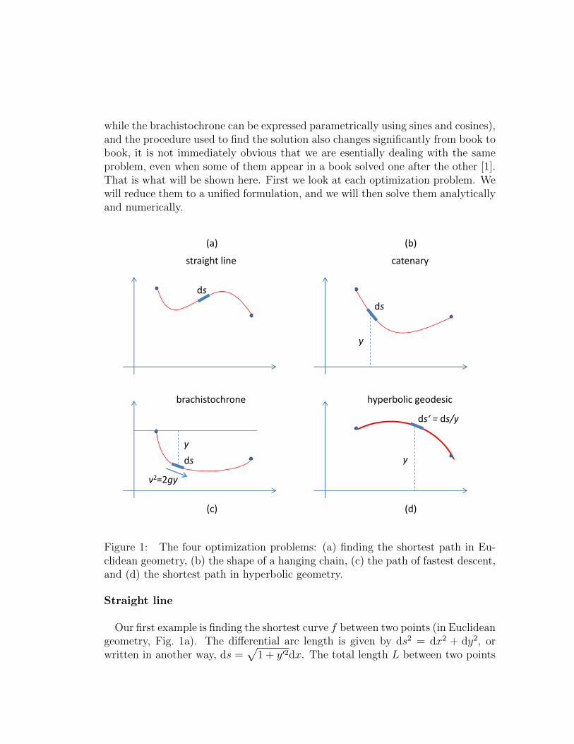
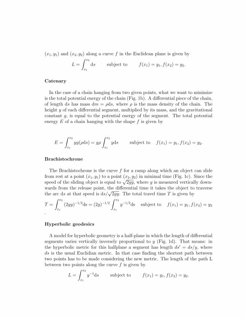
Figure 1: The four optimization problems: (a) finding the shortest path in Eu-clidean geometry, (b) the shape of a hanging chain, (c) the path of fastest descent,and (d) the shortest path in hyperbolic geometry.

Straight line

Our first example is finding the shortest curve f between two points (in Euclideangeometry, Fig. 1a). The differential arc length is given by ds2 = dx2 + dy2, orwritten in another way, ds =

√1 + y′2dx. The total length L between two points

(x1, y1) and (x2, y2) along a curve f in the Euclidean plane is given by

L =

∫ x2

x1

ds subject to f(x1) = y1, f(x2) = y2.

Catenary

In the case of a chain hanging from two given points, what we want to minimizeis the total potential energy of the chain (Fig. 1b). A differential piece of the chain,of length ds has mass dm = ρds, where ρ is the mass density of the chain. Theheight y of each differential segment, multiplied by its mass, and the gravitationalconstant g, is equal to the potential energy of the segment. The total potentialenergy E of a chain hanging with the shape f is given by

E =

∫ x2

x1

yg(ρds) = gρ

∫ x2

x1

yds subject to f(x1) = y1, f(x2) = y2.

Brachistochrone

The Brachistochrone is the curve f for a ramp along which an object can slidefrom rest at a point (x1, y1) to a point (x2, y2) in minimal time (Fig. 1c). Since thespeed of the sliding object is equal to

√2gy, where y is measured vertically down-

wards from the release point, the differential time it takes the object to traversethe arc ds at that speed is ds/

√2gy. The total travel time T is given by

T =

∫ x2

x1

(2gy)−1/2ds = (2g)−1/2∫ x2

x1

y−1/2ds subject to f(x1) = y1, f(x2) = y2

.

Hyperbolic geodesics

A model for hyperbolic geometry is a half-plane in which the length of differentialsegments varies vertically inversely proportional to y (Fig. 1d). That means: inthe hyperbolic metric for this halfplane a segment has length ds′ = ds/y, whereds is the usual Euclidian metric. In that case finding the shortest path betweentwo points has to be made considering the new metric. The length of the path Lbetween two points along the curve f is given by

L =

∫ x2

x1

y−1ds subject to f(x1) = y1, f(x2) = y2.

2 The general formulation

From what has been said it is obvious that the general formulation of the fourproblems above has the following form: Find the curve y that minimizes

k

∫ x2

x1

yαds = k

∫ x2

x1

yα√

1 + y′2dx subject to f(x1) = y1, f(x2) = y2,

(1)for α = 0 (Euclidean geometry),α = 1 (catenary),α = −1/2 (brachistochrone),and α = −1 (hyperbolic geodesic), and where k is a constant.

The general method for finding a solution to this problem of variational calculuswould be to use the Euler-Lagrange equation [2]. Given the problem of finding anoptimal value for an integral of the form∫ b

a

L(x, y, y′)dx

we can solve the differential equation

∂L

∂y− d

dx

∂L

∂y′= 0 (2)

in order to find a solution.

Since in our case the argument of the integral operator L = yα√

1 + y′2 haspartial derivative relative to x equal to zero, a simplification of the Euler-Lagrangeequation can be used, the so-called Beltrami’s identity:

L− y′ ∂L∂y′

= C (3)

Since∂

∂y′

√1 + y′2 =

y′√1 + y′2

applying Beltrami’s identity (Eq. 3) to our general formulation in Eq. 1 leads tothe following differential equation

yα√

1 + y′2 − yαy′2√1 + y′2

= C

which can be simplified toyα√

1 + y′2= C (4)

or equivalentlyy2α

1 + y′2=

y2αdx2

dx2 + dy2= C2, (5)

which is a first order nonlinear ordinary differential equation.

Proof of Beltrami’s Identity

From the Euler-Lagrange equation we know that

∂L

∂y=

d

dx

∂L

∂y′(6)

Using the chain rule we can express the derivative of L according to x as follows:

dL

dx= y′

∂L

∂y+ y′′

∂L

∂y′+∂L

∂x

In the case that ∂L/∂x = 0, we can simply write

dL

dx− y′∂L

∂y− y′′ ∂L

∂y′= 0.

Substituting the equivalent of ∂L/∂y from Eq. 6 in the second term above andgrouping, we obtain

dL

dx− (y′

d

dx

∂L

∂y′+ y′′

∂L

∂y′) = 0

But then the last two terms can be rewritten (using the differentiation productrule) as

dL

dx− d

dx

(y′∂L

∂y′

)=

d

dx

(L− y′ ∂L

∂y′

)= 0

and since the derivative is zero, we conclude that

L− y′ ∂L∂y′

= C

for a certain constant C.

It is easy to check that the solutions for the catenary, brachistochrone and circlefulfill the differential equations derived above (Eq. 4 and Eq. 5).

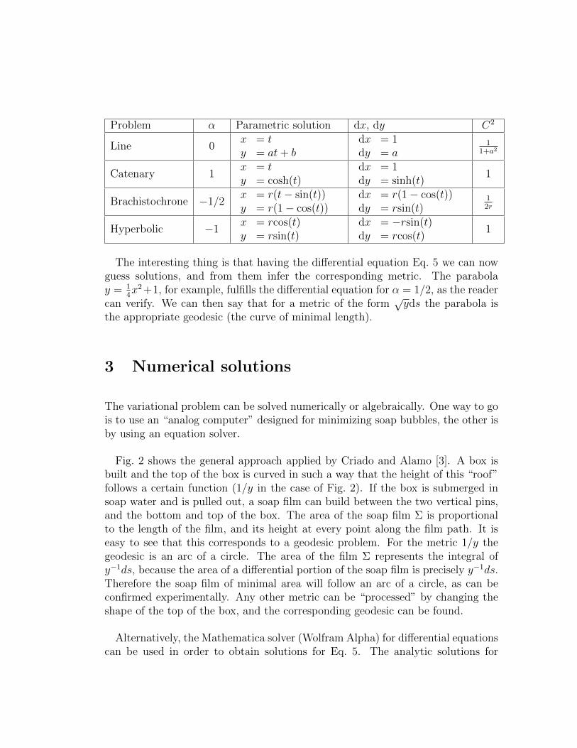
Problem α Parametric solution dx, dy C2

Line 0x = ty = at+ b

dx = 1dy = a

11+a2

Catenary 1x = ty = cosh(t)

dx = 1dy = sinh(t)

1

Brachistochrone −1/2x = r(t− sin(t))y = r(1− cos(t))

dx = r(1− cos(t))dy = rsin(t)

12r

Hyperbolic −1x = rcos(t)y = rsin(t)

dx = −rsin(t)dy = rcos(t)

1

The interesting thing is that having the differential equation Eq. 5 we can nowguess solutions, and from them infer the corresponding metric. The parabolay = 1

4x2+1, for example, fulfills the differential equation for α = 1/2, as the reader

can verify. We can then say that for a metric of the form√yds the parabola is

the appropriate geodesic (the curve of minimal length).

3 Numerical solutions

The variational problem can be solved numerically or algebraically. One way to gois to use an “analog computer” designed for minimizing soap bubbles, the other isby using an equation solver.

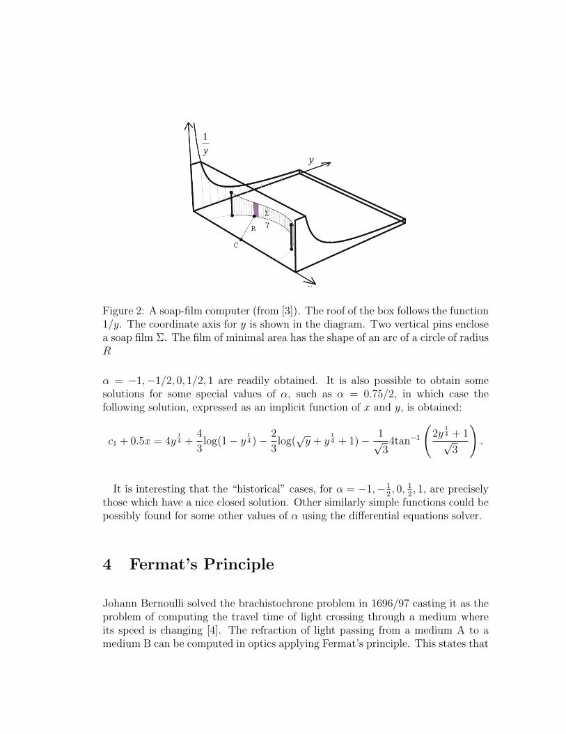
Fig. 2 shows the general approach applied by Criado and Alamo [3]. A box isbuilt and the top of the box is curved in such a way that the height of this “roof”follows a certain function (1/y in the case of Fig. 2). If the box is submerged insoap water and is pulled out, a soap film can build between the two vertical pins,and the bottom and top of the box. The area of the soap film Σ is proportionalto the length of the film, and its height at every point along the film path. It iseasy to see that this corresponds to a geodesic problem. For the metric 1/y thegeodesic is an arc of a circle. The area of the film Σ represents the integral ofy−1ds, because the area of a differential portion of the soap film is precisely y−1ds.Therefore the soap film of minimal area will follow an arc of a circle, as can beconfirmed experimentally. Any other metric can be “processed” by changing theshape of the top of the box, and the corresponding geodesic can be found.

Alternatively, the Mathematica solver (Wolfram Alpha) for differential equationscan be used in order to obtain solutions for Eq. 5. The analytic solutions for

y

1

y

Figure 2: A soap-film computer (from [3]). The roof of the box follows the function1/y. The coordinate axis for y is shown in the diagram. Two vertical pins enclosea soap film Σ. The film of minimal area has the shape of an arc of a circle of radiusR

α = −1,−1/2, 0, 1/2, 1 are readily obtained. It is also possible to obtain somesolutions for some special values of α, such as α = 0.75/2, in which case thefollowing solution, expressed as an implicit function of x and y, is obtained:

c1 + 0.5x = 4y14 +

4

3log(1− y

14 )− 2

3log(√y + y

14 + 1)− 1√

34tan−1

(2y

14 + 1√

3

).

It is interesting that the “historical” cases, for α = −1,−12, 0, 1

2, 1, are precisely

those which have a nice closed solution. Other similarly simple functions could bepossibly found for some other values of α using the differential equations solver.

4 Fermat’s Principle

Johann Bernoulli solved the brachistochrone problem in 1696/97 casting it as theproblem of computing the travel time of light crossing through a medium whereits speed is changing [4]. The refraction of light passing from a medium A to amedium B can be computed in optics applying Fermat’s principle. This states that

the travel time from a point A to a point B should be minimal, and if the velocityof light is different in medium A and medium B, then the optimal travel directionis such that

sin(θ1)

v1=sin(θ2)

v2

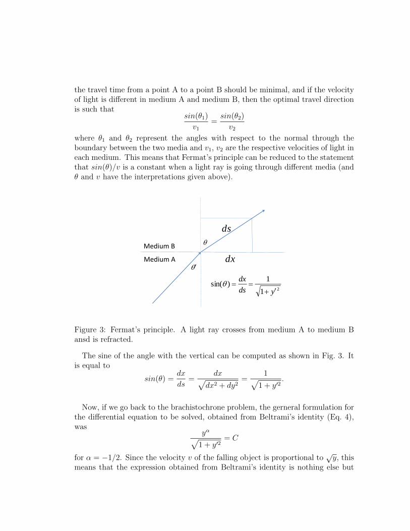
where θ1 and θ2 represent the angles with respect to the normal through theboundary between the two media and v1, v2 are the respective velocities of light ineach medium. This means that Fermat’s principle can be reduced to the statementthat sin(θ)/v is a constant when a light ray is going through different media (andθ and v have the interpretations given above).

dx

ds

Medium A

Medium B

21

1)sin(

yds

dx

Figure 3: Fermat’s principle. A light ray crosses from medium A to medium Bansd is refracted.

The sine of the angle with the vertical can be computed as shown in Fig. 3. Itis equal to

sin(θ) =dx

ds=

dx√dx2 + dy2

=1√

1 + y′2.

Now, if we go back to the brachistochrone problem, the gerneral formulation forthe differential equation to be solved, obtained from Beltrami’s identity (Eq. 4),was

yα√1 + y′2

= C

for α = −1/2. Since the velocity v of the falling object is proportional to√y, this

means that the expression obtained from Beltrami’s identity is nothing else but

Fermat’s principle! This is so because v ∼ √y and

y−1/2√1 + y′2

=sin(θ)√y

= C

Generalizing, we now interpret Eq. 4 in this form

yα√1 + y′2

=sin(θ)

y−α= C,

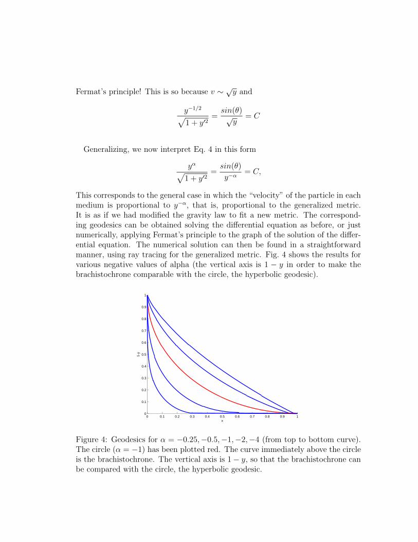
This corresponds to the general case in which the “velocity” of the particle in eachmedium is proportional to y−α, that is, proportional to the generalized metric.It is as if we had modified the gravity law to fit a new metric. The correspond-ing geodesics can be obtained solving the differential equation as before, or justnumerically, applying Fermat’s principle to the graph of the solution of the differ-ential equation. The numerical solution can then be found in a straightforwardmanner, using ray tracing for the generalized metric. Fig. 4 shows the results forvarious negative values of alpha (the vertical axis is 1 − y in order to make thebrachistochrone comparable with the circle, the hyperbolic geodesic).

0 0.1 0.2 0.3 0.4 0.5 0.6 0.7 0.8 0.9 10

0.1

0.2

0.3

0.4

0.5

0.6

0.7

0.8

0.9

1

x

1-y

Figure 4: Geodesics for α = −0.25,−0.5,−1,−2,−4 (from top to bottom curve).The circle (α = −1) has been plotted red. The curve immediately above the circleis the brachistochrone. The vertical axis is 1− y, so that the brachistochrone canbe compared with the circle, the hyperbolic geodesic.

5 Surfaces of revolution and designer geodesics

If we now let the the catenary rotate around the horizontal axis, we obtain a kindof curved cylinder. The surface of the side of the cylinder is minimal, since thecurve that minimizes

E = gρ

∫ x2

x1

yds subject to f(x1) = y1, f(x2) = y2

also minimizes

E = 2π

∫ x2

x1

yds subject to f(x1) = y1, f(x2) = y2.

This last integral represents the surface of a curved-cylinder of revolution withradius y1 and y2 at the basis and top. The minimal surface of revolution of thiskind is called the catenoid, because it is obtained rotating a catenary curve.

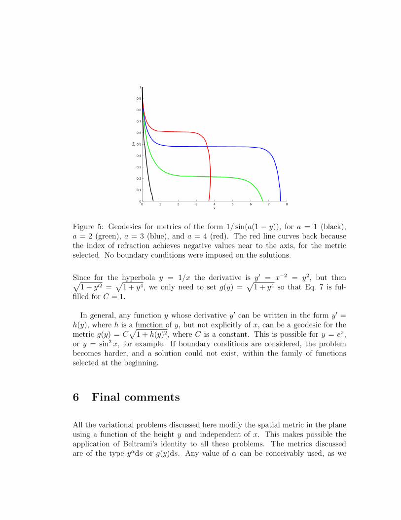
It is also possible to force almost any monotonous curve to be a geodesic. Fig. 5shows an example where the metric has been chosen not proportional to (1− y)α

but to functions of the form 1/ sin(a(1−y)), so that the velocity of “light” throughsuch a medium is forced to be proportional to C sin (a(1− y)). In Fig. 5 the valuesof a used are 1, 2, 3 and 4.

We can also just invert Fermat’s principle: given a desired geodesic, determinedby a sequence of angles θ1, θ2, . . . , θn relative to the vertical, of segments ds, an-chored at heights y1, y2, . . . , yn, Fermat’s principle tells us that we need velocitiesin each segment, such that vi = sin(θi)/C, for i = 1, . . . , n. The necessary refrac-tion indices for each layer can be computed from the relative change in angle θigoing through each layer.

In some cases we can even find the metric for a desired geodesic function analyt-ically. Assume that we want the hyperbola to be a geodesic for some metric g(y),which does not depend explicitly on x (so that we can apply Beltrami’s identity).In this case we want to minimize∫ x2

x1

g(y)√

1 + y′2dx

disregarding the boundary conditions. Substituting the metric g(y) for the metricyα in the differential Eq. 4 we are left with the condition

g(y)√1 + y′2

= C. (7)

0 1 2 3 4 5 6 7 80

0.1

0.2

0.3

0.4

0.5

0.6

0.7

0.8

0.9

1

x

1-y

Figure 5: Geodesics for metrics of the form 1/ sin(a(1 − y)), for a = 1 (black),a = 2 (green), a = 3 (blue), and a = 4 (red). The red line curves back becausethe index of refraction achieves negative values near to the axis, for the metricselected. No boundary conditions were imposed on the solutions.

Since for the hyperbola y = 1/x the derivative is y′ = x−2 = y2, but then√1 + y′2 =

√1 + y4, we only need to set g(y) =

√1 + y4 so that Eq. 7 is ful-

filled for C = 1.

In general, any function y whose derivative y′ can be written in the form y′ =h(y), where h is a function of y, but not explicitly of x, can be a geodesic for themetric g(y) = C

√1 + h(y)2, where C is a constant. This is possible for y = ex,

or y = sin2 x, for example. If boundary conditions are considered, the problembecomes harder, and a solution could not exist, within the family of functionsselected at the beginning.

6 Final comments

All the variational problems discussed here modify the spatial metric in the planeusing a function of the height y and independent of x. This makes possible theapplication of Beltrami’s identity to all these problems. The metrics discussedare of the type yαds or g(y)ds. Any value of α can be conceivably used, as we

did when solving numerically. The physical interpretation for such curious metricscorrespond to a plane with a continuously vertically varying index of refraction(positive or negative). Since the metric does not depend on x, the plane has beenfilled with horizontal layers with varying index of refraction (like a stack along they-direction of different transparent materials). This makes light rays curve alongthe geodesics of the resulting metric.

Materials with a varying index of refraction have been discussed in optics andhave become fashionable in the context of “cloaking devices” that curve lightrays around a disguised object [5]. Such materials represent a form of “analogcomputer” for geodesics ... without the soap water.

References

[1] C. Fox, An Introduction to the Calculus of Variations, Oxford University Press,Oxford, 1950.

[2] C. Lanczos, The Variational Principles of Mechanics, Dover Books, New York,1949.

[3] C. Criado, N. Alamo, ”Solving the brachistochrone and other variational prob-lems with soap film”, arXiv, http://arxiv.org/abs/1003.3924v3.

[4] H. Sussmann, J. Willems, “300 Years of Optimal Control: From the Brachys-tochrone to the Maximum Principle”, IEEE Control Systems, June 1997.

[5] M. Sarbort, “Non-Euclidean Geometry in Optics”, PhD Dissertation, MasarykUniversity, 2013.