Embed Size (px)
Citation preview

The Supplement Version 1.0
The SupplementTo the Carbon Credits (Carbon Farming Initiative—Measurement of Soil Carbon Sequestration in Agricultural Systems) Methodology Determination 2018
Version 1.0 – January 2018

The Supplement Version 1.0
ContentsPart A: Mapping Carbon Estimation Areas, exclusion zones, emissions accounting areas and sample locations....4
Part B: Developing Sampling Design.................................................................................................................... 5
1.0 Stratification...................................................................................................................................... 5
2.0 Assigning sampling locations.....................................................................................................7
Part C: Sampling.................................................................................................................................................. 8
1.0 Locating Sampling locations....................................................................................................... 8
Part D: Sample Preparation and Analysis........................................................................................................... 10
1.0 Samples: Single Cores, Composites, Layers and Sub-layers.......................................10
1.1 Separating and combining cores for analysis..................................................................10
1.2 Calculating appropriate 0-30cm and 0-xcm values for use in the equations in Schedule 1 of the Measurement of Soil Carbon Sequestration in Agricultural Systems Method Determination........................................................................................................11
2.0 Sample Preparation....................................................................................................................... 12
2.1. Homogenised sample.................................................................................................................12
2.2. Intact core.......................................................................................................................................13
3.0 Obtaining total soil organic carbon content......................................................................14
3.1 Dry Combustion analysis..............................................................................................................15
3.2 Spectroscopic modelling..............................................................................................................16
3.2.1 The spectrometer.........................................................................................................................................16
3.2.2 Spectroscopic measurements.......................................................................................................................17
3.2.3 Data for the spectroscopic modelling and validation...................................................................................193.2.3.1 Selection of the training set..................................................................................................................193.2.3.2 Selection of the validation set..............................................................................................................203.2.3.4 The prediction set.................................................................................................................................21
3.2.4 Determining the total organic carbon content of the training and validation soil samples with the reference analytical method.................................................................................................................................................21
3.2.4.1 Accuracy of reference analytical approach...........................................................................................22
3.2.5 Developing the spectroscopic model............................................................................................................223.2.5.1 Preparing the data for modelling..........................................................................................................223.2.5.2 Spectral transformations, pre-processing and pre-treatments.............................................................233.2.5.3 Corrections for the effects of water on spectra....................................................................................243.2.5.4 Statistical transformation of the reference analytical data...................................................................243.2.5.5 Calculating the multivariate spectroscopic model................................................................................253.2.5.6 Model diagnosis....................................................................................................................................253.2.5.7 Identification and omission of outliers.................................................................................................273.2.5.8 Optimising and assessing the model.....................................................................................................27
2

The Supplement Version 1.0
3.2.5.9 Model uncertainties..............................................................................................................................273.2.5.10 Independent validation.......................................................................................................................283.2.5.11 assessing the accuracy of the model...................................................................................................283.2.5.12 Using the spectroscopic model to estimate the organic carbon content of the prediction set..........29
3.2.6 Estimation of soil organic carbon in subsequent sampling rounds after the baseline..................................30
3.2.7 Software.......................................................................................................................................................30
3.2.8 Troubleshooting – sources of error...............................................................................................................32
4.0 Soil bulk density............................................................................................................................. 33
4.1 Soil bulk density using conventional laboratory approach........................................33
4.2 Soil bulk density using Gamma-ray attenuation sensing...........................................34
4.2.1 The densitometer.........................................................................................................................................34
4.2.2 Setting up the densitometer.........................................................................................................................35
4.2.3 Measurements of soil bulk density using gamma-ray attenuation...............................................................35
Part E: Emissions Factors................................................................................................................................... 37
Part F: Additional Reporting Requirements........................................................................................................ 41
Part G: Glossary................................................................................................................................................ 44
Part H: References............................................................................................................................................ 47
3

The Supplement Version 1.0
Part A: Mapping Carbon Estimation Areas, exclusion zones, emissions accounting areas and sample locationsRequirements:
i. It is a requirement that a geospatial map is produced.ii. It is a requirement that the geospatial map is submitted
electronically. iii. It is a requirement that the following features are clearly
identifiable:a. Each CEA b. Exclusion zonesc. Emissions accounting areasd. For each sampling round:
Strata boundaries Intended sample locations (in the sampling design) Actual sample locations (as taken in the field)
iv. It is a requirement that project proponents use one or more of the following sources of data to delineate the boundaries of Carbon Estimation Areas, exclusion areas and emissions accounting areas:
a. Differential Global Positioning System (GPS)b. Field surveys and samplingc. Orthorectified aerial photographsd. Orthorectified satellite imagerye. Cadastral database.
v. It is a requirement to provide spatial data that meets the following requirements:
a. Has a horizontal accuracy of at least 10 meters at 95 per cent threshold in accordance with the Intergovernmental Committee on Surveying and Mapping (ICSM) - Australian Map and Spatial Data Horizontal Accuracy Standard 2009.
vi. It is a requirement that carbon estimation area boundaries are delineated with a maximum resolution of ± four meters. To be clear, a resolution as small as possible is preferable and must not exceed ± four meters.
Recommendations:i. It is recommended that project proponents assess the
appropriateness of the dataset(s) (selected in requirement iv. of this Part) for the intended use against the following criteria:
a. Ageb. Scale
4

The Supplement Version 1.0
c. Resolutiond. Accuracye. Classification, aggregation, generalisation systemsf. Integrity of datasetg. Relevance to the proposed ERF activity
5

The Supplement Version 1.0
Part B: Developing Sampling DesignRequirements:
i. It is a requirement that a sampling plan is developed and documented for the baseline sampling round.
ii. It is a requirement that the sampling plan is updated in subsequent sampling rounds to incorporate changes to the sampling plan compared to the previous sampling round.
iii. It is a requirement to document any changes to the sampling plan.
iv. It is a requirement that the sampling plan includes details of carbon estimation areas, exclusion zones, emissions accounting areas, strata and sample locations, as outlined in this part.
Recommendations:
i. It is recommended that proponents develop a sampling plan in consultation with information that is well documented in the peer reviewed literature. Some examples of useful resources include:
a. Sampling protocols published in the peer reviewed literature (e.g. de Gruijter et al, 2016; Viscarra Rossel et al., 2016b).
b. The R Project (https://www.r-project.org/)c. Generating spatially and statistically representative maps
of environmental variables to test the efficiency of alternative sampling protocols (Cunningham et. al, 2017)
d. Soil carbon stock in the tropical rangelands of Australia: Effects of soil type and grazing pressure, and determination of sampling requirement (Pringle et. al, 2011)
e. A geostatistical method to account for the number of aliquots in composite samples for normal and lognormal random variables (Orton et. al, 2015)
f. CFI Equal area stratification soil sampling design guidelines (https://environment.gov.au/system/files/pages/b341ae7a-5ddf-4725-a3fe-1b17ead2fa8a/files/cfi-soil-sampling-design-method-and-guidelines.pdf).
ii. It is recommended to consider the following when deciding on your sampling design:
a. Number of samples you can afford per CEA
6

The Supplement Version 1.0
b. How much you know about the soil carbon variability across the project area.
1.0 Stratification
Requirements:i. It is a requirement that each CEA is divided into three or more
strata. ii. It is a requirement that strata do not overlap.
iii. It is a requirement to report if strata are equal (within 5%) or unequal in area across a given CEA.
iv. It is a requirement that strata boundaries are delineated by generating a set of spatial coordinates that define the geographic limits of the land included within each stratum by using a geographic information system to generate spatial data files.
v. It is a requirement that spatial data files documenting the strata boundaries are created for each sampling round, even if the strata boundaries remain the same.
vi. It is a requirement, if strata are not equal in size, that samples are not composited across strata.
vii. It is a requirement, if samples are composited across strata, that strata have an equal area and that the strata boundaries remain fixed through time. For the purpose of this requirement, strata will be considered to have an equal area if there is no more than 5% difference in area (based on the average strata size) between the smallest and largest strata in a CEA.
viii. If strata have an equal area, it is a requirement that strata boundaries remain fixed for all sampling rounds in which strata with equal area are used. It is possible to swap between strata with equal or unequal area between sampling rounds. Figure 1a demonstrates an example of stratification of a single CEA over a number of sampling rounds that would be allowed. Figure 1b shows one that would not be allowed as when the equal area stratification is repeated in t2 the strata do not have the same boundaries.
7
(a)
t3 sampling roundt2 sampling roundt1 sampling roundt0 sampling round

The Supplement Version 1.0
Figure 1: (a) stratification designs of a CEA at four subsequent sampling rounds where repeated equal area strata designs have the same strata boundaries; (b) stratification designs of a CEA at four subsequent sampling rounds where repeated equal area strata designs do not have the same strata boundaries.
Recommendations:
i. It is recommended that if strata are unequal in size that: stratification is undertaken to minimise the variation in soil
carbon within each stratum. the land is homogenous with respect to land management (eg.
inter-row vs. intra-row in cropping systems), soil type, land form or other variables.
variables highly correlated to carbon content are used to inform stratification of each carbon estimation area into individual strata
each carbon estimation area is restratified for each sampling round as better information (with respect to recommendation i of this section) becomes available.
ii. It is recommended that if strata are equal in size that: samples are composited across strata within a given carbon
estimation area the variation in soil carbon within each carbon estimation
area is minimised.
8
(b)
t3 sampling roundt2 sampling roundt1 sampling roundt0 sampling round

The Supplement Version 1.0
2.0 Assigning sampling locations
Requirements:i. It is a requirement that sample locations are determined prior to
any core extraction in a given stratum for a given sampling round.
ii. It is a requirement that the geographic point location of assigned sampling points are recorded along with the units used.
iii. It is a requirement that the precision of each sampling location (or alternative sampling location) is:
a. if longitude and latitude are used – a minimum of five decimal places; or
b. if eastings and northings are used – a minimum of three decimal places.
iv. It is a requirement that within each stratum, sampling locations are assigned using a pseudo-random number generator with a defined seed number.
v. It is a requirement that there are at least three sample locations within each stratum.
vi. It is a requirement, if compositing and equal area stratification are chosen, that an equal number of sample locations are assigned to each stratum.
vii. It is a requirement that a soil core is taken at each sample location (or alternative sample location) assigned in this part, and is prepared, analysed and the results reported as per Part D.
9

The Supplement Version 1.0
Part C: Sampling1.0 Locating Sampling locations
Requirements:i. It is a requirement that a GPS device with a minimum accuracy
of ± four meters is to be used to locate the sampling location in the field.
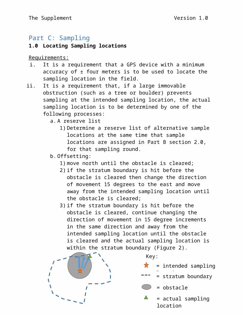
ii. It is a requirement that, if a large immovable obstruction (such as a tree or boulder) prevents sampling at the intended sampling location, the actual sampling location is to be determined by one of the following processes:
a. A reserve list1) Determine a reserve list of alternative sample locations
at the same time that sample locations are assigned in Part B section 2.0, for that sampling round.
b. Offsetting:1) move north until the obstacle is cleared; 2) if the stratum boundary is hit before the obstacle is
cleared then change the direction of movement 15 degrees to the east and move away from the intended sampling location until the obstacle is cleared;
3) if the stratum boundary is hit before the obstacle is cleared, continue changing the direction of movement in 15 degree increments in the same direction and away from the intended sampling location until the obstacle is cleared and the actual sampling location is within the stratum boundary (Figure 2).
Figure 2: Example of determining an alternative sampling location within a stratum in the presence of an obstacle using the offsetting approach.
iii. It is a requirement that both the intended and the actual sampling locations are reported (even if they are the same).
10
Key:
= actual sampling location
= obstacle
= stratum boundary
= intended sampling location
The Supplement Version 1.0
2.0 Extracting cores
Requirements: i. It is a requirement that the sample location is cleared of living
plants, plant litter and surface rocks, prior to core extraction.ii. It is a requirement that the nominated sampling depth is a
minimum of 30cm.iii. It is a requirement that soil samples to the minimum depth of
30cm are extracted in a single core. However the core can be split into any number of individual depth layers after removal.
iv. It is a requirement that, if sampling occurs beyond the minimum depth, soil from the 0-30cm layer and the 30+cm layer are extracted separately or separated prior to the sample preparation step (unless part D, section 2.2 applies).
v. It is a requirement that the nominated sampling depth is the same at all sample locations in a given carbon estimation area. The only exception to this is where the nominated sampling depth cannot be reached due to bedrock or impenetrable layers. In this situation, the actual sampling depth must be recorded.
vi. It is a requirement that, if the soil profile is altered (incorporating substances external to the profile, or vertically altering the profile – eg. tilling, clay delving, water ponding) the sampling depth must be at least 10cm below the depth of profile alteration.
vii. It is a requirement that the nominated sampling depth used in the baseline sampling round is used in all subsequent sampling rounds. The only exception to this is (if the nominated sampling depth is greater than 30cm): the nominated sampling depth may be reduced to 30cm depth at a later stage unless requirement vii. of this section applies. If requirement vii. of this section applies, nominated sampling depth must not be reduced.
viii. It is a requirement that the inner cutting edge of the coring device has a minimum diameter of 38mm.
ix. It is a requirement to have a clean coring device. Coring devices must only be cleaned with water.
x. It is a requirement to use only water to assist with insertion and extraction of the coring device.
xi. It is a requirement that there is a minimum of one year, and a maximum of five years between the median day of one sampling round and the median day of the next.
11
The Supplement Version 1.0
xii. It is a requirement that all cores are extracted from a given carbon estimation area for a given sampling round over no more than 60 calendar days. Note: In exceptional circumstances preventing sampling within these timeframes, a project proponent may apply to the Regulator to seek an extension of time to carry out the carbon estimation area sampling round.
xiii. It is a requirement that the time between successive sampling rounds (median day to median day) does not differ by more than two years.
xiv. It is a requirement to report the day, month and year that a given sampling round for a given carbon estimation area starts and finishes.
xv. It is a requirement to report the median day of the sampling round.
xvi. It is a requirement that all sampling rounds occur at least 24 months after the application of non-synthetic fertiliser.
xvii. It is a requirement that soil extracted is analysed for all soil properties separately for the 0-30cm layer and the 30+cm layer (unless part D, section 2.2 applies).
Part D: Sample Preparation and Analysis1.0 Samples: Single Cores, Composites, Layers and Sub-layers
1.1 Separating and combining cores for analysis.
Requirements:i. It is a requirement to decide and record whether the soil organic
carbon stock change will be determined on either: a) 0-30cm depth only; orb) 0-30cm and 30-x cm depths.
ii. It is a requirement, if requirement i. option b) of this section is chosen, that sample preparation is undertaken separately for each depth layer (ie. 0-30cm and 30-x cm).
iii. It is a requirement, if a given depth layer is broken into multiple sub-layers for analysis, the sub-layers do not extend over the 30cm depth boundary.
iv. It is a requirement to decide and record whether the samples will be analysed as either:
a) individual cores; or b) composite samples.
v. If requirement iv. option b of this section is chosen, it is a requirement to report the type of compositing:
12

The Supplement Version 1.0
a) across strata compositing (must not be used if strata are unequal in size); or
b) within strata compositing.
vi. It is a requirement, if strata are equal in size, and compositing is chosen, that in each composite sample there is exactly one core from every stratum within a carbon estimation area.
vii. If requirement iv. option a of this section is chosen, it is a requirement to undertake analysis on a sample prepared in one of the following ways:
a) homogenised sample (section 2.1 of this part); orb) in-tact cores (section 2.2 of this part).
viii. If requirement iv. option b of this section is chosen, it is a requirement to undertake analysis on a homogenised sample (section 2.1 of this part).
Recommendations:
i. It is recommended, if strata are equal in size, that composites are formed from soil cores from across all the strata, rather than analysing individual cores.
13

The Supplement Version 1.0
1.2 Calculating appropriate 0-30cm and 0-xcm values for use in the equations in Schedule 1 of the Measurement of Soil Carbon Sequestration in Agricultural Systems Method Determination.
Requirements:i. If multiple sub-layers are analysed individually, it is a
requirement to derive the mass(M a) (oven dry equivalent) for the equations in schedule 1 of the Measurement of Soil Carbon Sequestration in Agricultural Systems Method Determination by calculating the cumulative soil mass (CSM) for the 0-xcm depth layer using equation 1:
M a=∑sl=1
n
( tsl×BDsl×100 ) Equation 1
Where:M a= The actual cumulative soil mass of the 0-X cm depth layer (t soil/hectare). This is the value of M a to be used in the equations in schedule 1.sl = A given sub-layer, where the 0-xcm depth is split into multiple sub-layers for analysis. If x is greater than 30cm, sl must be at least 2. t sl = The thickness of the sublayer (cms).BDsl = The Bulk density of the sub layer (g/cm3) determined in accordance with Part D, section 4.0.Note: this mass is oven dry equivalent. If using the conventional method to determine bulk density, then oven dry mass will have been used in that calculation, and the value can be used directly. If the bulk density has been determined using gamma attenuation, the water content has already been corrected for (Part D. Section 4.0.) and the value can be used directly.
ii. If the soil is sampled to a depth, such that x is greater than 30cm, it is a requirement to derive input M i for the equations in schedule 1 of the Measurement of Soil Carbon Sequestration in Agricultural Systems Method Determination by calculating the cumulative soil mass for the 0-30cm depth layer using equation 1.
iii. If multiple sub-layers are analysed individually, it is a requirement to derive input OC i for the equations in schedule 1 of the Measurement of Soil Carbon Sequestration in Agricultural
14

The Supplement Version 1.0
Systems Method Determination by calculating the cumulative soil mass for the 0-xcm depth layer using equation 2:
OC i=∑sl=1
n
¿¿ Equation 2
Where:
OC i = The weighted average mass of carbon in the 0-x cm depth layer grams). This is the value of OC i to be used in the equations in schedule 1.sl = A given sub-layer, where the 0-xcm depth is split into multiple sub-layers for analysis. If x is greater than 30cm, sl must be at least 2.t sl = The thickness of the sublayer (cms). BDsl = The Bulk density of the sub layer (g/cm3) determined in accordance with Part D, section 4.0.M a = The actual cumulative soil mass of the 0-X cm depth layer (t soil/ha). This is the value of M a to be used in the equations in schedule 1.OCsl = The organic carbon content (%C of oven dry mass) of a given sub-layer, where the 0-x is split into multiple sub-layers for analysis.
iv. If the soil is sampled to a depth, such that x is greater than 30cm, it is a requirement to derive input OC i for the equations in schedule 1 of the Measurement of Soil Carbon Sequestration in Agricultural Systems Method Determination by calculating the cumulative soil mass for the 0-30cm depth layer using equation 2.
v. It is a requirement, that for each sub-layer on which carbon content is determined, that there is a value of bulk density determined (in accordance with Part D, section 4.0).
2.0 Sample Preparation2.1. Homogenised sample
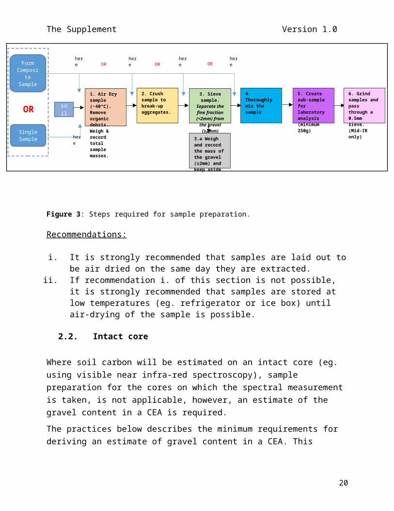
Requirements:i. It is a requirement to adhere to the process in figure 3 for
sample preparation of homogenised samples.ii. It is a requirement that the process in Figure 3 is followed
separately for each layer that is sampled. This can either be for
15

The Supplement Version 1.0
each depth layer (ie. 0-30cm and 30-xcm) or if a given depth layer is broken into multiple sub-layers, for each sub-layer.
iii. It is a requirement if mid-IR is used to analyse the sample for carbon content that step 6 (of figure 3) is undertaken.
iv. It is a requirement to report the volume of the soil sample (either single soil core or composite sample) based on the volume of the soil core/s.
v. It is a requirement that composite samples (if used) are formed before step 4 in figure 3 (thoroughly mix the sample).
vi. It is a requirement to report (if composite samples are used) between which steps the composite sample was formed. For example, the cores might be dried and crushed as individual cores, then form a composite sample between step 2 and step 3.
vii. It is a requirement that each soil sample (core or composite) is dried separately.
viii. It is a requirement to report the mass (air-dry) of the sub-sample used for laboratory analysis.
Figure 3: Steps required for sample preparation.
Recommendations:
i. It is strongly recommended that samples are laid out to be air dried on the same day they are extracted.
ii. If recommendation i. of this section is not possible, it is strongly recommended that samples are stored at low temperatures (eg. refrigerator or ice box) until air-drying of the sample is possible.
2.2. Intact core
16
OR
here
herehereherehere OROROR
Single Sample
Form Composite
Sample
3.a Weigh and record the mass of the gravel (≥2mm) and keep aside
2. Crush sample to break-up aggregates.
1. Air Dry sample (~40°C). Remove organic debris. Weigh & record total sample masses.
3. Sieve sample.Separate the fine fraction
(<2mm) from the gravel (≥2mm)
4. Thoroughly mix the sample
5. Create sub-sample for laboratory analysis (minimum 250g)
6. Grind samples and pass through a 0.5mm sieve. (Mid-IR only)
soil

The Supplement Version 1.0
Where soil carbon will be estimated on an intact core (eg. using visible near infra-red spectroscopy), sample preparation for the cores on which the spectral measurement is taken, is not applicable, however, an estimate of the gravel content in a CEA is required.The practices below describes the minimum requirements for deriving an estimate of gravel content in a CEA. This estimate is applied through time as it is assumed the gravel content of the CEA will not change.Requirements:
i. It is a requirement that the gravimetric gravel content is determined on the larger of either:
a. 3 cores per stratum orb. 30% of the soil cores extracted for carbon analysis.
ii. It is a requirement to measure the gravel content of these samples in the 0-30 cm depth layer.
iii. It is a requirement to measure the gravel content of these samples in the 30-x cm depth layer, where x = the depth to which carbon is analysed.
iv. It is a requirement that gravimetric gravel content for each sample is determined by sieving the crushed, oven-dry soil sample and weighing the portion that does not pass through the 2mm sieve by following steps 1-3 and 3a in Figure 3.
v. It is a requirement that the total mass of gravel of a CEA is determined in accordance with the following equations:
¿C EAi=¿ i×
ACEA
ACS×100 Equation 3
¿CEA=(∑i=1
n
¿C EAii)ni
Equation 4
Where:¿C EAi is the total mass of gravel for a CEA – calculated using the mass of gravel in a single sample (Tonnes)
gGi is the total gravel per sample, i, in grams, determined in accordance with the requirements of this section.ACEA is the total area of the CEA in hectares.
17

The Supplement Version 1.0
ACS is the area of the cutting surface of the coring device (cm2).
gGCEA is the total mass of gravel for a CEA – calculated using average mass of gravel across all samples (Tonnes)ni is the number of cores analysed for gravel content.
Recommendations:i. It is recommended that proponents measure the gravel content
of all of the soil cores in a CEA as this will provide estimates of gravel with smaller errors.
ii. It is strongly recommended, if recommendation i. is not possible, to measure the gravel content of as many cores as possible as making more measurements will result in more accurate estimates of mean gravel and thus smaller uncertainties.
3.0 Obtaining total soil organic carbon content
Requirements:i. It is a requirement that organic carbon content of each stratum
is determined by following the requirements in either section 3.1 or section 3.2 of this part.
ii. It is a requirement that if section 3.2 of this part is chosen, that section 2.1 and section 3.1 of this part are followed for the preparation and analysis of the training and validation sets with the following differences.
a. It is a requirement that preparation and analysis is undertaken on individual samples (not composite samples).
b. It is a requirement that the soil sample corresponding to each spectra (refer to section 3.2.4 requirement iii. of this part) in the training and validation sets are prepared and analysed separately.
3.1 Dry Combustion analysis
The following requirements and recommendations apply if dry combustion analysis is selected as the analysis technique for obtaining total soil organic carbon content.
Requirements:
i. It is a requirement that dry combustion analysis is undertaken on a soil prepared as per section 2.1 of this part.
ii. It is a requirement that analysis of organic carbon content is undertaken by a laboratory that is certified for organic carbon
18

The Supplement Version 1.0
analysis by the Australasian Soil and Plant Analysis Council (ASPAC).
iii. It is a requirement that the method used to analyse organic carbon content is a dry combustion approach which has been certified by ASPAC.
iv. It is a requirement that the method used to analyse organic carbon content is a dry combustion approach and has been accredited, for that laboratory, by the National Association of Testing Authorities (NATA) under ISO-IEC 17025 (chemical testing).
v. It is a requirement to adhere to the following process in Figure 4.
Figure 4: combustion analysis and gravimetric water content (g water per g oven dry soil).
Recommendations:
i. It is recommended, that if dry combustion analysis is being undertaken to calibrate samples analysed using mid-IR, subsample A (figure 3) should be ground to as close to 0.5mm as possible.
3.2 Spectroscopic modelling
19
Split sub-sample into portions(sub-sample A & sub-sample B)
Subsample AFine-grind to
<0.5mm
Subsample BWeigh and record air-dry mass (less container) to 2 decimal places
Subsample BOven dry at (105°C) to constant mass
Subsample BPlace in desiccator to cool
Subsample BWeigh and record oven-dry mass (less container) to 2 decimal places
Calculate & report
gravimetric water content to 2
decimal places
Subsample ACarry out organic carbon analysis as per NATA accredited organic
carbon method
Calculate & report organic
carbon % (based on the oven dry
mass)
The Supplement Version 1.0
The practices described below provide a guide for the standardised methods for the visible and infrared measurements of soil and the multivariate modelling of soil spectra used in determining the total organic carbon content of soil in a carbon estimation area (CEA).The practices apply to analyses conducted in the visible–near infrared spectral region (vis–NIR: 400–2500 nm, equivalent to 25,000–4000 cm-1) and in the mid infrared region (mid-IR: 2500–25,000 nm, equivalent to 4000–400 cm-1).The practices, describe physical instruments and procedures for recording and treating soil organic carbon (C) data and spectra, for developing multivariate spectroscopic models, for validating them and for assessing their performance. The instructions cover techniques that are routinely applied in quantitative soil spectroscopy using undisturbed, coarse and finely ground soil.
3.2.1 The spectrometerRequirements:
i. It is a requirement that the spectrometer used, is able to measure spectra with the following wavelengths:
a. 400–2500 nm if a combined visible–near infrared technique is used;
b. 700–2500 nm if only near infrared spectroscopy is used;c. 2500–16600 nm if mid infrared spectroscopy is used.
ii. It is a requirement that spectrometers be installed and operated in accordance with the instructions of the instrument manufacturer.
iii. It is a requirement that the spectral resolution of the instrument(s) are recorded and reported.
iv. It is a requirement that the wavelength/wavenumber interval in the spectra (i.e. the spacing between wavelengths/wavenumbers of the spectra) be:
a. 10 nm for the vis–NIR or NIRb. 8 cm-1 for the mid-IR
v. It is a requirement that instrument calibration is performed as per manufacturer’s instructions and using their recommended standard materials and practices or using one of the following standards:
a. For vis–NIR, Spectralon Diffuse Reflectance Standards (https://www.labsphere.com/).
b. For mid-IR, gold or silicon carbide (SiC) standards.
20

The Supplement Version 1.0
vi. It is a requirement that the spectrometer control parameters be set to:
a. For vis–NIR and NIR: record and average 30 readings per soil sample measurement, and 50 readings per calibration with Spectralon reference material.
b. For mid-IR record and average 64 readings per soil sample and 64 readings per calibration with gold or silicon carbide (SiC) reference material.
vii. It is a requirement that the spectrometer control parameters be maintained constant for the collection of all spectra of samples in the project.
viii. It is a requirement that the spectrometer be calibrated every 10 min or once every 30 measurements if sequentially measuring many samples in blocks of time.
ix. It is a requirement that if the measurement configuration uses an external calibration standard, then to ensure that the same configuration is used for the soil sample measurements.
x. It is a requirement to ensure that the spectrum of the reference represents 100% reflection at all wavelengths across the particular spectral range, with no more than 5% of noise. Often noise is present towards the edges of the sensor’s response and towards the extreme of the wavelength range. If the reference spectrum shows noise that exceeds this threshold, check the setup, clean the reference standard material (following manufacturer’s instructions) and repeat the calibration. If it persists, check with the instrument manufacturer for repair.
Recommendations:
i. Most instruments include the necessary accessories to perform the spectroscopic measurements. It is recommended that proponents use these accessories following manufacturer’s guidelines with reference to the guidelines provided by the global spectral library project (Viscarra Rossel et al 2016a).
ii. It is recommended that instrument performance is tested as per manufacturer’s recommendations and instructions at the time of instrument calibration.
iii. It is recommended that the instruments are monitored on a periodic (6 monthly basis) following either:
a. the instrument manufacturer’s recommendations and instructions or
21
The Supplement Version 1.0
b. a relevant approach published in the scientific peer reviewed literature such as the guidelines provided by the global spectral library project (Viscarra Rossel et al 2016a).
iv. It is recommended that the same spectrometer be used for the baseline and subsequent rounds of sampling. If a different spectrometers are used in the different rounds of sampling it is strongly recommended that the spectra be measured by strictly following the same protocols and that spectral pre-processing algorithms (e.g. first derivatives) or calibration transfer methods (Fearn, 2001), such as direct standardisation or piecewise direct standardisation be used to address the differences in the spectra.
3.2.2 Spectroscopic measurementsThe procedures described are for site-specific (or local) multivariate spectroscopic modelling performed with the spectra of soil samples from only the particular CEA. However, if proponents have access to a larger spectral library with a wider range of soil types and from different environments, they may augment their site-specific models with data from the spectral library if the additional data complements the local set and improves the accuracy of the models as measured by the RMSE and R2 of the independent validation set.Requirements:
i. It is a requirement that the spectra are recorded from a soil samples prepared in one of the following ways:
a. the surface of intact soil cores (air-dry or at field condition), at intervals (see requirement 3.2.2(iii.) of this part) from the soil surface to the desired depth (prepared as per section 2.2 of this part); or
b. homogenised soil (from a particular depth layer) that was dried, crushed, ground and sieved (as per section 2.1 of this part). For vis–NIR the samples are ground to pass a ≤2mm sieve and for mid-IR the samples are ground to pass a ≤0.5 mm sieve.
ii. It is a requirement to use requirement 3.2.2 (i.)(b.) of this part if the instrument is a mid-IR spectrometer.
22

The Supplement Version 1.0
iii. If requirement 3.2.2 (i.)(a.) of this part is chosen, it is a requirement that spectra are recorded at intervals of:
a. no more than 5 cm between spectra from the soil surface to the desired depth; and
b. no less than 1 cm between spectra from the soil surface to the desired depth.
iv. It is a requirement that the spectra of all of soil samples in a CEA are recorded with the same spectrometer.
v. It is a requirement that spectral outliers are identified from the full set of CEA spectra, using published algorithms in the scientific literature (Martens H & Næs T, 1989).
vi. It is a requirement that if spectral outliers are identified, the soil samples are remeasured with the spectrometer for verification.
vii. If after verification spectral outliers are present, it is a requirement that they be removed from the acquired set of CEA spectra before selection of training and validation sets in sections 3.2.3.1. and 3.2.3.2 of this part, respectively.
viii. It is a requirement that if after identification and verification of spectral outliers as in requirements 3.2.2(v.) and (vi.) of this part, they are removed, their sample numbers are saved for reporting.
Recommendations:
i. It is recommended that if requirement 3.2.2 (i.)(a.) of this part is chosen, the surface of the soil core is inspected prior to measurements to check for smearing of the soil surface, in which case, the soil surface should be ‘brushed’ with a bristle brush only to remove the smearing and to expose the true soil.
3.2.3 Data for the spectroscopic modelling and validationOnce the soil is sampled, all of the soil samples must be measured with the spectrometer as in section 3.2.2. of this part. From all of the CEA spectra, a training set and a validation set of soil samples need to be identified independently of each other. Once the training and validation sets are selected, the remaining CEA spectra are called the prediction set. The soil samples of the training and validation set need to be analysed to determine their soil organic carbon concentration using the analytical method described section 3.1 of this Part.
23

The Supplement Version 1.0
The training set is used to develop the spectroscopic model by applying multivariate mathematics to calibrate the spectra against the soil organic carbon concentration derived from the combustion analysis of the same samples. The validation set is independent from the training set and is used to test the accuracy of the model’s estimates (i.e. the bias and imprecision). This is done by statistically comparing the spectroscopic estimates of soil organic carbon concentration in the validation samples to the results from the combustion analysis of the same samples. The validated model (i.e. that derived from the training set after validation) is used to estimate the total organic carbon concentration and uncertainty for the prediction set, which is made up of the spectra of the remaining soil samples in the CEA.
3.2.3.1 Selection of the training setThe number of spectra that are required to develop the spectroscopic model depends on the complexity and variability of the soil in the CEA. Requirements:
i. It is a requirement that, once all of the spectra have been recorded from all of the soil samples in the CEA as in requirement 3.2.2(iv) of this part, a training set is selected using a method published in the scientific peer-reviewed literature (e.g. the Kennard-Stone (Kennard & Stone, 1969), Duplex (Snee, 1977), Select (Shenk & Westerhaus 1991) algorithms)
ii. It is a requirement that the training set consists of a minimum of either:
a. 40 soil samples with spectra when the total number of samples in a CEA is ≤ 200 or
b. 20% of the total number of soil samples with spectra in a CEA when the total number of samples in a CEA is ≥ 200.
iii. It is a requirement that the published method chosen in requirement 3.2.3.1(i.) of this part ensures that the training set contains pairs of spectra and reference analytical values:
24

The Supplement Version 1.0
a. that characterise the entire range of all of the project spectra that are to be analysed using the spectroscopic model.
Recommendations:
i. It is recommended that as the complexity and variability of the soil in the CEA increases, the number of spectra chosen to form the training set increases proportionally. Proponents should opt for using more (rather than less) training data for the spectroscopic modelling during the baseline round.
3.2.3.2 Selection of the validation setThe number of spectra required to independently validate a spectroscopic model depends on the complexity and variability of the soil in the CEA.Requirements:
i. It is a requirement that the validation set is selected independently of the training set in section 3.2.3.1 of this part, and using a method that is published in the scientific peer-reviewed literature (e.g. methods suggested in requirement 3.2.3.1(i.) of this part)
ii. It is a requirement that the validation set consists of a minimum of either:
a. 20 soil samples with spectra when the total number of samples in a CEA is ≤ 200; or
b. 10% of the total number of soil samples with spectra in a CEA when the total number of samples in a CEA is ≥ 200.
iii. It is a requirement that the method chosen in requirement 3.2.3.2(i.) of this part ensures that the validation set contains pairs of spectra and reference analytical values that characterise the entire range of all of the CEA spectra that are to be analysed using the spectroscopic model.
Recommendations:
i. It is recommended that as the complexity and variability of the soil in the CEA increases, the number of spectra chosen to form the validation set increases proportionally.
25

The Supplement Version 1.0
ii. It is recommended that proponents opt for using more data (rather than less) for validating the spectroscopic model.
26

The Supplement Version 1.0
3.2.3.4 The prediction set
Requirements:
i. It is a requirement that the remaining spectra, after the training and independent validation sets have been taken for the spectroscopic modelling, are put together to form the prediction set.
3.2.4 Determining the total organic carbon content of the training and validation soil samples with the reference analytical method
Requirements:
i. It is a requirement that for each spectrum in the training and validation sets, the corresponding soil sample be analysed to determine the soil organic carbon content of the using the reference analytical method.
ii. It is a requirement that the soil samples in the training and validation sets are prepared and analysed following sections 2.1 and 3.1 of this part.
iii. It is a requirement, if requirement 3.2.2. (i.)(a.) of this part is chosen, that for a given spectrum, the corresponding soil sample analysed using the reference analytical approach is:
a. at least the width of the spectrometer measurement spot size (width of orange band in Figure 5); and
b. at most the distance of halfway between the locations where two adjacent spectra were recorded, to halfway between the locations where the next two spectra were recorded (distance between two dotted lines in Figure 5).
27

The Supplement Version 1.0
Figure 5. A soil core showing the spot size from where a spectrum of a particular depth layer is recorded, and the minimum and maximum width of the soil core subsamples that are cut, crushed, sieved and sent to the analytical laboratory to measure the soil organic C content.
iv. It is a requirement, if requirement 3.2.2 (i.)(b.) is chosen, that for a given spectrum, the soil sample analysed using the reference analytical approach is subsampled and prepared and analysed following sections 2.1 and 3.1.
v. It is a requirement that if requirement 3.2.2 (i.)(b.) is chosen, both the spectroscopic and the reference analytical measurements be made on the same prepared (air-dry, crushed, sieved, ground) soil sample.
vi. It is a requirement that the composition of the soil samples taken for spectroscopic measurements and for reference laboratory analyses be representative of the soil at the time the samples are taken, and that the composition is maintained during transport for preparation and analysis in the laboratory.
3.2.4.1 Accuracy of reference analytical approachThe accuracy of the spectroscopic estimate of organic C is dependent on the accuracy of the reference analysis values used for training and validating the spectroscopic model. Requirements:
i. It is a requirement that all total soil carbon concentrations are expressed on the basis of oven dry soil mass.
28

The Supplement Version 1.0
Recommendations:
i. It is recommended at least five subsamples are selected at random and sent to the laboratory as ‘blind duplicates’ for assessment of accuracy of the reference analysis values, using a measure of the standard error of laboratory measurements (SEL). The accuracy of the spectroscopic method will be limited by that of the reference analytical method, as such, the accuracy of the spectroscopic estimate can never exceed the accuracy of the reference method.
ii. It is strongly recommended that if the SEL of the blind duplicates is larger than the analytical error reported by the laboratory that proponents contact the laboratory and ask for the samples to be reanalysed.
3.2.5 Developing the spectroscopic model
3.2.5.1 Preparing the data for modelling
Requirements:
i. It is a requirement that once the total organic carbon concentrations of the training and validation soil samples are returned from the laboratory, they are matched with their corresponding spectra to develop the spectroscopic model.
Recommendations:
i. If proponents have a larger spectral library with a wider range of soil types and from different environments, they may use it to augment their CEA-specific training data set (see section 3.2.3.1 of this part) to develop a spectroscopic model with the combined data. It is recommended that they only do this if the additional data complements the local set and improves the accuracy of the models when assessed against the independent validation set.
3.2.5.2 Spectral transformations, pre-processing and pre-treatments
Various algorithms can be applied to the spectra prior to development of the multivariate spectroscopic model to remove random noise,
29

The Supplement Version 1.0
remove undesired spectral variations due to light scatter effects and variations in effective path length during measurements.Requirements:
i. It is a requirement that any implemented spectral transformations, pre-processing and/or pre-treatments, are applied consistently to all the training set spectra, the validation set spectra and prediction set spectra acquired from within the CEA.
Recommendations:
i. It is recommended that the effects of random noise, undesired spectral variations due to light scatter effects and variations in effective path length during measurement are corrected by testing different spectral transformations, pre-processing and pre-treatments that are reported in the peer-reviewed scientific literature. This might result in an improvement of the signal to noise.
ii. It is recommended that different spectral transformations, pre-processing and pre-treatments algorithms reported in the peer-reviewed scientific literature are tested and applied to the spectra prior to development of the multivariate spectroscopic model to test which, if any, will most effectively achieve recommendation 3.2.5.2(i.) of this part. Most spectroscopic software packages (see section 3.2.7 of this part) will enable the implementation of these techniques. These could include but are not limited to:
a. transformation to test is the conversion of reflectance (R) spectra to apparent absorbance (A), where A = Log(1/R);
b. spectral pre-processing to test can include the multiplicative scatter correction (MSC) (Geladi, McDougel & Martens 1985), standard normal variate (SNV) (Barnes, Dhanoa & Lister, 1989), digital filters to smooth the spectra such as mean or median filters, moving average, the Savitski-Golay filter (Savitzky & Golay, 1964), first and second derivatives, or other methods that are published in the peer-reviewed scientific literature;
c. pre-treatment includes mean centring the spectra, which involves calculating the arithmetic mean spectrum of the
30

The Supplement Version 1.0
data set and subtract that mean from each spectrum. The result is that the mean centred spectra will have a mean of zero.
3.2.5.3 Corrections for the effects of water on spectraRequirements:
i. It is a requirement that soil spectra are corrected for water using a method that has been tested and verified by publication in the scientific peer-reviewed literature (e.g. External Parameter Orthogonalisation (EPO) (Minasny et al, 2011), or direct standardisation (DS) (Ji, Viscarra Rossel & Shi, 2015) if:
a. the spectroscopic measurements are made on soil cores or homogenised and ground soil from soils that are wetter than their air dry condition; or
b. the spectroscopic measurements are made on soil cores that are at field condition; or
c. a larger spectral library was used to augment the site-specific data for the modelling, then the site-specific field spectra that are wet and at field condition will need to be corrected for water using a method such as EPO or DS.
Recommendations:
i. It is recommended that the transformation matrix (Barnes, Dhanoa & Lister, 1989), or transfer set (Savitzky & Golay, 1964), to make the corrections for water using either EPO or DS are made on a site-specific basis, following the experiments described by Barnes, Dhanoa & Lister (1989) and Savitzky & Golay (1964).
3.2.5.4 Statistical transformation of the reference analytical data
Requirements:
i. It is a requirement that any transformations performed on the training set are also performed on the validation set.
Recommendations:
i. It is strongly recommended that the organic carbon concentration data be transformed to approximate normal
31

The Supplement Version 1.0
distribution before modelling, if its statistical distribution is (positively) skewed and the algorithm used for modelling assumes normally distributed data. For example, the data may be transformed using square root or logarithmic transformations, depending on the data and the degree of transformation required.
3.2.5.5 Calculating the multivariate spectroscopic modelThe spectroscopic modelling relates the spectra measured on the training set to the soil organic carbon concentration values and validates the model on the validation set. Development of the validated model allows the soil organic carbon concentration in the prediction set, (i.e. the spectra of the remaining samples in the CEA) to be estimated using the spectroscopic model.
Requirements:
i. It is a requirement that the spectroscopic model is derived using techniques that have been tested and verified for soil spectroscopic modelling by publication in the scientific peer-reviewed literature.
ii. It is a requirement that the peer-reviewed technique used:
a. follows best-practice as indicated in the publications that describe the algorithm and its implementation, and/or the software being used; and
b. ensures the data used in the model does not violate the statistical assumptions of the model; and
c. is capable of producing a model that can be validated with the independent validation set as described in section 3.2.5.10 of this part, below.
Recommendations:
i. It is recommended that one of the following techniques is used for the spectroscopic modelling:
a. partial least squares regression (PLSR) (Martens & Næs, 1989); or
b. principal components regression (PCR) (Martens & Næs, 1989); or
32

The Supplement Version 1.0
c. other methods that have been reported in the peer-reviewed scientific literature to be successful for spectroscopic modelling are described and compared in this publication (Viscarra Rossel & Behrens, 2010), and may be for example, support vector machines (SVM), regression trees (RT), Cubist, random forest (RF), or Bayesian methods.
3.2.5.6 Model diagnosis
Requirements:
i. It is a requirement to diagnose the spectroscopic model and departures from the statistical assumptions of the model being used, by calculating the residuals of each specimen in the training set (model residuals = observed – estimated) and deriving a plot of these residuals on the y-axis and the estimated soil property concentrations on the x-axis.
ii. It is a requirement to report this plot. If all assumptions about the model are correct, then the model has a good diagnosis and a plot of residuals against the estimated values should show a horizontal band as illustrated in Figure 6a. Deviations from this, for example as illustrated in Figure 6b, indicates dependence on the predicted value, suggesting incorrect numerical calculations or that an intercept term has been omitted from the model. If the pattern of residuals are like those in Figure 6c, it indicates that the variance is non-constant (or heteroscedastic) and increases with each increment of the predicted value. In this case, transformation of the data, as in section 3.2.5.4 of this part, might be required. The pattern of residuals in Figure 6d indicates non-linear trends in the data, indicating the need for transformation or curvilinear modelling methods.
33

The Supplement Version 1.0
Figure 6. Possible residual plots for model diagnosis. Residuals can be located anywhere between the dashed lines. Adapted from Kalivas & Gemperline (2006) (Kalivas & Gemperline, 2006).
Recommendations:
i. It is recommended that the residuals plot in Figure 5a be also used to help with the identification of outliers. For instance, outliers might fall outside two standard deviations from the mean of the residuals. However, omission of outliers must be performed following the requirements in section 3.2.5.7 of this part.
3.2.5.7 Identification and omission of outliersRequirements:
i. It is a requirement to identify analytical reference data outliers in the training and validation sets using methods that have been tested and verified by publication in the scientific literature (Martens & Næs, 1989), for example using Studentized residuals (Cook & Weisberg, 1982). Outliers here refer to a sample whose
34

The Supplement Version 1.0
analytical value is unusual given its spectra. Outliers to look for are:
a. analytical values that represent an extreme concentration (i.e. either very large or very small carbon concentration) relative to the remainder of the training set (these data will have a very large leverage on the model); and
b. samples whose estimated values are significantly different to the reference analytical values. This indicates either an error in the reference analytical value, a sample mislabelling issue, or failure of the model.
ii. It is a requirement to report the total number of samples and their sample identification numbers, which have been identified and omitted as outliers.
3.2.5.8 Optimising and assessing the modelOptimisation is important to prevent the model from under fitting or over fitting.Requirements:
i. It is a requirement that a cross-validation procedure, such as leave-one-out or k-fold cross validation, be used to estimate the optimum model parameters to use. For example, optimising the number of latent variables to use in the PLSR model, or using other modelling methods, it could be the number of trees, committees, nodes, basis functions, or other method-specific parameter that needs to be optimised to derive the optimal spectroscopic model.
ii. It is a requirement that the optimised model is assessed using the cross validation RMSE and R2 and that these statistics are reported.
3.2.5.9 Model uncertaintiesRequirements:
i. It is a requirement to derive modelling uncertainties be derived using methods that are reported in the peer-reviewed scientific literature (see recommendation 3.2.5.9(i.) of this part).
ii. It is a requirement that the uncertainties are represented by 95% confidence limits.
35

The Supplement Version 1.0
Recommendations:
i. It is recommended that modelling uncertainties be derived using a Monte Carlo method such as bootstrapping (Viscarra Rossel, 2007), or using Bayesian methods.
3.2.5.10 Independent validation Validation of the spectroscopic model using the independent validation set enables thorough assessment of the model to ensure that it performs up to the expectations derived at the model development and model assessment statistics section 3.2.5.8 of this part.Requirements:
i. It is a requirement that the spectroscopic model derived using the training data set is validated using the independent validation data set (selected in section 3.2.3.2 of this part).
ii. It is a requirement that the estimated values on the validation set (derived using the spectroscopic model) are compared statistically to the values obtained by the reference analytical method for the validation set.
iii. It is a requirement to assess and report the accuracy, precision and bias of the model, which can be measured by the root mean squared error (RMSE), the standard deviation of the error (SDE) and the mean error (ME), respectively.
iv. There is support for a general rule that overall soil variation influences the accuracy of the predictions (Stenberg et al., 2010). Thus it is a requirement that the RMSE value be reported together with the mean and standard deviation of the soil organic C data of the training data set.
v. It is a requirement that the assessment includes the coefficient of the determination, R2, for the relationship between predicted and measured organic carbon contents, and that this value is reported.
Recommendations:
i. It is recommended that the sRMSE of the independent validation be calculated. The sRMSE will show the improvement that might be gained compared to using simply the mean as the prediction.
36

The Supplement Version 1.0
Smaller values indicate less residual variance and better model validation.
3.2.5.11 assessing the accuracy of the modelRequirements:
i. If the independent model validation statistics (see section 3.2.5.10 of this part) are not within the range of values reported in the literature (see recommendation 3.2.5.11(i.) of this part), it is a requirement to return to section 3.2.3.1 of this part and select an additional set of soil samples (this does not need to be as many as originally specified for selection of training or validation sets) to augment and extend the range of the training set and proceed with sections 3.2.3.2 of this part onwards.
ii. If after the second selection (requirement 3.2.5.11(i.) of this part), the model validation statistics are not within the range of values reported in the literature (see recommendation 3.2.5.11(i) of this part), then it is a requirement that estimation of total organic C is not conducted using spectroscopy.
Recommendations:
i. It is recommended that the independent model validation RMSE and R2 values be compared to those reported in the peer reviewed-scientific literature. A review of the literature (Viscarra Rossel et. al, 2016a) has shown that the accuracy, measured with the RMSE, of soil organic C predictions at the field- and farm-scales, using vis–NIR spectra, ranges from 0.1–1.0% soil organic C, with the median being 0.3% soil organic C. The R2 values of soil organic C predictions at field- and farm-scales reported in the literature, using vis–NIR spectra range from 0.6 to 0.96, with a median R2 of 0.86.
3.2.5.12 Using the spectroscopic model to estimate the organic carbon content of the prediction set
Requirements:
i. It is a requirement that if the spectra of the training and validation data sets were transformed, pre-processed and/or pre-treated, as in section 3.2.5.2, all of the remaining spectra in the prediction set be transformed, pre-processed and/or pre-treated in exactly the same manner.
37

The Supplement Version 1.0
ii. It is a requirement that the spectroscopic model that was optimised (see section 3.2.5.8) and validated (see section 3.2.5.10) is applied on all of the spectra in the prediction set, to estimate the soil organic carbon concentration of those samples.
iii. It is a requirement that the optimised spectroscopic model be used to estimate the uncertainty of the estimates in the prediction set and to represented them as 95% confidence limits.
iv. It is a requirement that if the model was developed on the logarithmic scale, that the estimates of the prediction set be
back-transformed to the original scale using:
y=e(ψ+
1N ∑
i=1
N
( ψi−ψ i)2
2 ) Equation 5
where y are the back-transformed data, ψ are the estimates of the soil organic C, ψ are the observed values, for each sample i, both on the logarithmic scale, and the numerator in the exponent represents the mean squared error (MSE) of the model, or the MSE of the independent validation set.
v. It is a requirement that the spectroscopic model be used to predict the organic C content of all of the CEA spectra, which includes the training data itself, the validation set and the prediction set. This will ensure that all observations in the training, validation and prediction sets have the same measurement error.3.2.6 Estimation of soil organic carbon in subsequent sampling rounds after the baseline
Requirements:
i. It is a requirement that, in any particular sampling round after the baseline survey, the spectra of all soil samples in a CEA collected at the particular sampling round, be recorded with the spectrometer as described in section 3.2.2.1 of this part.
ii. It is a requirement that from all of the CEA spectra, a validation set is selected as described in section 3.2.3.2 of this part.
iii. It is a requirement that any implemented spectral transformations, pre-processing and/or pre-treatments as in sections 3.2.5.2–3.2.5.3 of this part, are applied consistently to the validation set spectra in requirement 3.2.6(ii.) of this part.
iv. It is a requirement that the same spectroscopic model that was used to predict the organic C content of the soil of the baseline survey is also used to predict the organic C content of the soil in this validation set.
38

The Supplement Version 1.0
v. It is a requirement that for each spectrum in this validation set, the corresponding soil sample be analysed to determine the soil organic carbon content using the reference analytical method, as in section 3.2.4 of this part.
vi. It is a requirement that the accuracy of the predictions be assessed as described in sections 3.2.5.10 and 3.2.5.11 of this part. If the validation statistics are not within the range of values reported in the literature (see recommendation 3.2.5.11(i.) of this part), it is a requirement to return to section 3.2.3.1 of this part and select an additional set of soil samples to augment and extend the range of the training set of the baseline round and proceed the development of the spectroscopic model for the new round as described in section 3.2.5 of this part.
3.2.7 SoftwareRequirements:
It is a requirement that, using this document and procedures outlined in sections 3.2.1 to 3.2.6 of this part, proponents develop a workflow to perform the spectroscopic measurements, modelling and estimation. The procedures are summarised in Figure 7.
39
The Supplement Version 1.0
Figure 7. Flow diagram of the procedures to estimate the organic C content of soil using visible–infrared spectra.
Recommendations:
i. It is recommended that proponents use one of the software platforms that were specifically developed for spectroscopic data analysis, modelling and estimation. There are a number of stand-alone commercial and shareware software with point-and-click graphical user interfaces:
a. Unscrambler - http://www.camo.com/rt/Resources/spectroscopy.html
b. GramsAI - https://www.thermofisher.com/order/catalog/product/INF-15000
40

The Supplement Version 1.0
c. WinISI - http://www.foss.com.au/industry-solution/products/winisi/
d. ParLeS - http://www.sciencedirect.com/science/article/pii/S0169743907001347
As well as these, there are more general statistical software, some of which are programmable and with specific modules for spectroscopic data analysis and modelling:
a. JMP - https://www.jmp.com/b. Matlab - https://au.mathworks.com c. R - https://www.r-project.org
3.2.8 Troubleshooting – sources of error
This section contains only recommendations.
Recommendations:
i. It is recommended that proponents use Table 1 as a source of information and possible solutions for general sources of error in the spectroscopic measurements and multivariate modelling.
Table 1 General sources of error
Source of error Possible solution
Poor spectrometer performance Conduct instrument performance tests as per manufacturer’s instructions and section B in this document.
Inhomogeneous soil sample Ensure appropriate drying, crushing, sieving and mixing procedures. If measurements are taken from on a soil core, ensure that the core is not smeared.
Chemical and physical variation of soil sample with time Perform measurements soon after sample collection and ensure appropriate storage of the air-dry soil sample.
Spectroscopy insensitive to property being modelled Try different spectral range (e.g. mid-IR) or defer back to reference analytical technique
Inadequate population in training set Review criteria and method for selection of training set. Test an alternative method for the selection.
Outliers degrade the training model Employ robust outlier detection methods and omit outlying data, or alternatively remeasure the soil sample for verification.
Reference analytical data errors Analyse additional blind duplicate samples to test the ‘true’ error of the laboratory.
41

The Supplement Version 1.0
Poor model Check model cross validation statistics and compare to independent validation statistics – they should be similar. Check that independent validation set is representative of the population.
Errors in the multivariate analysis Prepare a logical workflow that is checked by someone with experience on the use of the methods and software.
4.0 Soil bulk density
Requirements:i. It is a requirement that bulk density is determined following
either section 4.1 or 4.2 of this part.
4.1 Soil bulk density using conventional laboratory approach
Requirements:
i. It is a requirement to calculate the volume of the sample on which carbon analysis was undertaken. This will be:
If analysis is undertaken on individual cores,
V=tsl× ACS Equation 6
Or, if the sample is a composite sample,
V= ∑(allcores)
(t sl× ACS) Equation 7Where:
V= Volume of the sample (cm3)t sl= thickness of the sublayer (cm)ACS= Area of the cutting surface (cm2)All cores = all cores in the sample (if composite sampling used)
ii. It is a requirement to calculate the total oven dry mass of the sample:
MOD=M gravel+M ¿ 2mm Equation 8Where:
MOD= Total oven dry mass of the sample (g)M gravel= the mass of the gravel (>2mm fraction) in the soil sample (g) M ¿2mm=the oven-dry (equivalent) mass of the fraction of soil sample <2mm (g)
42

The Supplement Version 1.0
iii. It is a requirement to calculate the oven-dry (equivalent) mass of the <2mm fraction of soil:
M ¿2mm=M AD<2mm
1+ƟmEquation 9
Where:M ¿2mm= the oven-dry (equivalent) mass of the fraction of soil
sample <2mm (g)M AD< 2mm = the air-dry mass of the fraction of the soil sample that
is <2mm (g)Ɵm= the gravimetric water content of the <2mm air-dry sub-sample (g water/ g oven dry soil mass) as reported by the laboratory.
iv. It is a requirement to calculate the air-dry mass of the <2mm fraction of soil:
M AD<2mm=MAD−M gravel Equation 10Where:
M AD< 2mm = the air-dry mass of the fraction of the soil sample that is <2mm (g)M AD= the air-dry mass of the soil sample (g)M gravel= the mass of the gravel (>2mm fraction) in the soil sample (g)
v. It is a requirement to calculate the Bulk Density of the sample. This will be:
BD=MOD
VEquation 11
Where:BD = the bulk density of the sample (g/cm3)MOD= Total oven dry mass of the sample (g) – calculated usingV = Volume of the sample (cm3)
4.2 Soil bulk density using Gamma-ray attenuation sensing
The practices below cover a guide for the standardised methods of measuring soil bulk density using gamma-ray attenuation axially through a cylindrical soil core sample. The practices describe the instrumentation and procedures for measuring and collecting data.
43
The Supplement Version 1.0
The theory and principle of the measurements can be found elsewhere (Lobsey & Viscarra Rossel, 2016).
4.2.1 The densitometer
Requirements:i. It is a requirement that the gamma-ray attenuation instrument
consists of a radioactive source, a scintillation detector and a data logger.
ii. It is a requirement that the activity of the radioactive source be selected to measure soil core samples with densities ranging from 0.5–2.65 g cm-3.
iii. It is a requirement that the purchase and operation of the radioactive source follow guidelines and requirements set by the relevant State and Territory regulatory bodies or the Australian Radiation Protection and Nuclear Safety Agency (ARPANSA).
iv. It is a requirement that the instrument is operated in accordance with the instructions of the instrument manufacturer.
Recommendations:i. It is recommended that the radioactive energy source is a 137Cs
with an activity of 185MBq and a peak gamma energy of 0.662MeV.
ii. It is recommended that the scintillation detector be a NaI scintillation crystal of 25-mm diameter and 25-mm length.
iii. It is recommended that instrument performance and decay of the radioactive source be tested regularly or as per manufacturer’s instructions.
4.2.2 Setting up the densitometer Requirements:
i. It is a requirement that the gamma ray source and detector are mounted and aligned with the centre of the core (with diameters ranging from 40–85 mm) so that the gamma source emits a narrow beam of collimated gamma-rays at a particular energy (e.g. 137Cs at 0.662 MeV), and that these photons pass axially through the soil core and are recorded by the detector on the other side (Figure 8).
44

The Supplement Version 1.0
Figure 8. Setup of the densitometer for measuring soil core samples.
4.2.3 Measurements of soil bulk density using gamma-ray attenuation
Requirements:i. It is a requirement that on the setup of the instrument, a once-
off experiment be performed to determine the mass attenuation coefficient of soil, s, and water, w, using the particular instrument and setup and using:
μs=1x ρb
ln( I 0
I )Equation 12
where I is in counts s-1 and is taken as the average of the four measurements, x is the measured longitudinal thickness of the core in cm, b is the bulk density the core determined by conventional analytical methods and is given in g cm-3. The value of I0 is determined directly with no soil core sample in the attenuation path. For the calculation of w use Equation 12, replacing s with w, replacing the soil core with a cylindrical container with pure water that has the same shape and diameter of the soil core, and replacing b with w.
ii. It is a requirement that the instrument be monitored daily at the start of the measurements using standards of known density. Standards to use must have the same shape and diameter as the soil core and must expand the density range between 0.5–1.8 g cm-3, e.g. standard materials with known densities of 1.0, 1.5 and 1.7 g cm-3.
iii. It is a requirement that the measurement be recorded only when the counts per second measured by the detector have stabilised.
iv. It is a requirement that, if using soil spectroscopy to measure the total soil organic carbon content of the soil core, both the gamma and spectroscopic measurement be taken at exactly the same depth interval (Figure 9).
45

The Supplement Version 1.0
Figure 9. Sensor measurements at the same depth interval on the soil core sample.
v. It is a requirement that at least one measurement be taken at intervals of a maximum of 5 cm and a minimum of 1 cm, or the width of the spectrometer spot size (see section 3.2.3.4) between gamma readings from the soil surface to the desired depth, to ensure that the measurements are representative of the depth layer of interest (e.g. measurements taken at 5 cm intervals there are 6 measurements within the 0–30 cm layer).
vi. It is a requirement that Equation 13 be used to determine the bulk density of the soil being measured. If the measurements are made on oven-dry soil core samples then is zero, the portion of Equation 13 located to the right of the minus sign becomes zero and the measurements are of the soil bulk density. However, if the measurements are made on soil cores that are wet or at field condition, then independent measures of are required to solve Equation 13. The bulk density of the soil, b, can be derived using:
ρb=1x μs
ln( I 0
I )−μw
μsρw θ Equation 13
where I is the incident radiation at the detector, I0 is the un-attenuated radiation emitted from the source and x is the sample thickness in cm, s is the mass attenuation coefficient of dry soil in cm2 g-1, w is the mass attenuation coefficient of soil water at 0.662 MeV (reported values for the w in the literature, for similar configurations have a mean of 0.0832 cm2 g-1 and standard deviation 0.0006 cm2 g-1), w is the density of water (taken as 1 g cm-3), and represents the volumetric water content of the soil in cm-3.
Recommendations:
46

The Supplement Version 1.0
i. It is recommended that the independent estimate of be acquired using spectroscopic modelling, following the procedures described the ‘Total soil organic carbon’ section above and following the method described by Lobsey & Viscarra Rossel (2016).
ii. It is recommended that using the gamma-ray sensors, as well as bulk density, cumulative soil mass (CSM) is calculated as described by Viscarra Rossel and Behrens (2010).
Part E: Emissions FactorsStandard Parameters and Emissions Factors for the Carbon Credits (Measurement of Soil Carbon Sequestration in Agricultural Systems) Methodology Determination 2018
Table 1: Sheep (g) Emission Factors (kg CO2-e/head/day) State (i) Season (k) Class (j)
Rams Wethers Maiden Ewes
(intended for
breeding)
Breeding Ewes
Other Ewes
Lambs & Hoggets
NSW/ACT Spring 1.01 0.83 0.60 0.79 0.76 0.32 Summer 0.80 0.58 0.44 0.52 0.54 0.30 Autumn 0.77 0.61 0.48 0.57 0.55 0.37 Winter 0.88 0.70 0.58 0.68 0.65 0.46
Queensland Spring 0.50 0.43 0.31 0.37 0.39 0.20 Summer 0.58 0.52 0.38 0.42 0.47 0.25 Autumn 0.63 0.55 0.41 0.49 0.50 0.23 Winter 0.58 0.49 0.35 0.41 0.47 0.26
South Spring 1.01 0.87 0.65 0.71 0.69 0.51Australia Summer 0.67 0.62 0.49 0.52 0.52 0.42
Autumn 0.44 0.38 0.32 0.36 0.34 0.15 Winter 0.78 0.67 0.58 0.68 0.61 0.37
Tasmania Spring 1.28 0.77 0.64 0.80 0.71 0.26 Summer 0.90 0.52 0.43 0.47 0.47 0.24 Autumn 0.89 0.59 0.53 0.60 0.58 0.43 Winter 0.71 0.43 0.45 0.55 0.47 0.41
Victoria Spring 0.89 0.76 0.63 0.74 0.64 0.32 Summer 0.62 0.52 0.43 0.48 0.47 0.28 Autumn 0.75 0.60 0.50 0.58 0.58 0.40 Winter 0.55 0.46 0.37 0.44 0.46 0.34
Western Spring 0.99 0.79 0.66 0.75 0.72 0.42Australia Summer 0.61 0.51 0.42 0.47 0.46 0.29
47

The Supplement Version 1.0
Autumn 0.37 0.27 0.33 0.38 0.26 0.12 Winter 0.86 0.64 0.60 0.75 0.66 0.32
Table 2: Beef Cattle (g) Emission Factors (kg CO2-e/head/day)State/Region (i)
Season(k)
Class (j)
Bulls >1
Bulls <1
Steers <1
Cows1 to 2
Cows >2
Cows <1
Steers >1
Northern Spring 4.537 2.488 2.742 2.648 3.224 2.250 2.766Territory Summer 5.732 2.107 3.151 3.047 4.611 1.933 3.221 Autumn 5.510 2.455 3.336 3.203 4.177 2.130 3.367 Winter 5.055 2.417 2.703 2.983 3.387 2.174 2.742
NSW/ACT Spring 4.508 1.651 3.921 3.343 5.422 1.612 3.982 Summer 5.169 2.824 4.315 4.273 5.106 2.661 4.463 Autumn 5.142 3.210 4.365 4.051 4.669 2.957 4.495 Winter 4.854 3.150 4.183 3.997 4.508 2.989 4.251
Queensland Spring 6.031 1.874 3.804 3.141 5.560 1.639 3.857
Summer 6.510 2.814 4.664 4.057 5.208 2.584 4.852 Autumn 5.174 3.368 4.754 4.180 4.022 3.097 4.885 Winter 4.650 3.781 4.316 4.174 3.874 3.304 4.373
South Spring 7.417 3.645 4.267 4.608 5.379 3.266 4.434Australia Summer 5.648 3.839 3.881 4.142 4.471 3.407 3.940 Autumn 4.375 1.916 3.547 3.265 4.586 1.719 3.662 Winter 5.974 2.812 3.967 4.305 4.914 2.538 4.184
Tasmania Spring 6.690 2.424 4.952 4.344 6.899 2.228 5.416 Summer 6.373 5.389 4.677 4.029 5.682 2.429 4.848 Autumn 6.564 3.495 4.836 3.901 4.509 2.844 5.134 Winter 5.752 3.141 4.289 4.306 4.267 2.689 4.563
Victoria Spring 8.050 4.047 5.716 5.576 6.805 3.952 6.158 Summer 6.090 3.147 4.610 4.410 4.685 2.900 4.722 Autumn 5.808 1.885 4.034 3.496 5.607 1.873 4.171 Winter 6.429 2.522 4.560 3.793 5.452 2.388 4.932
Western South Spring 7.687 5.374 5.834 5.433 6.052 4.101 6.064Australia West Summer 5.482 4.116 4.199 4.547 4.520 3.459 4.257 Autumn 5.325 1.875 3.299 3.357 4.588 1.714 3.331 Winter 6.282 3.223 4.115 3.733 5.336 2.654 4.311
Pilbara Spring 3.544 1.694 3.244 2.806 3.722 1.616 3.290 Summer 5.117 2.421 4.050 3.742 4.342 2.335 4.174 Autumn 5.339 3.145 4.057 3.460 3.850 3.061 4.146
48
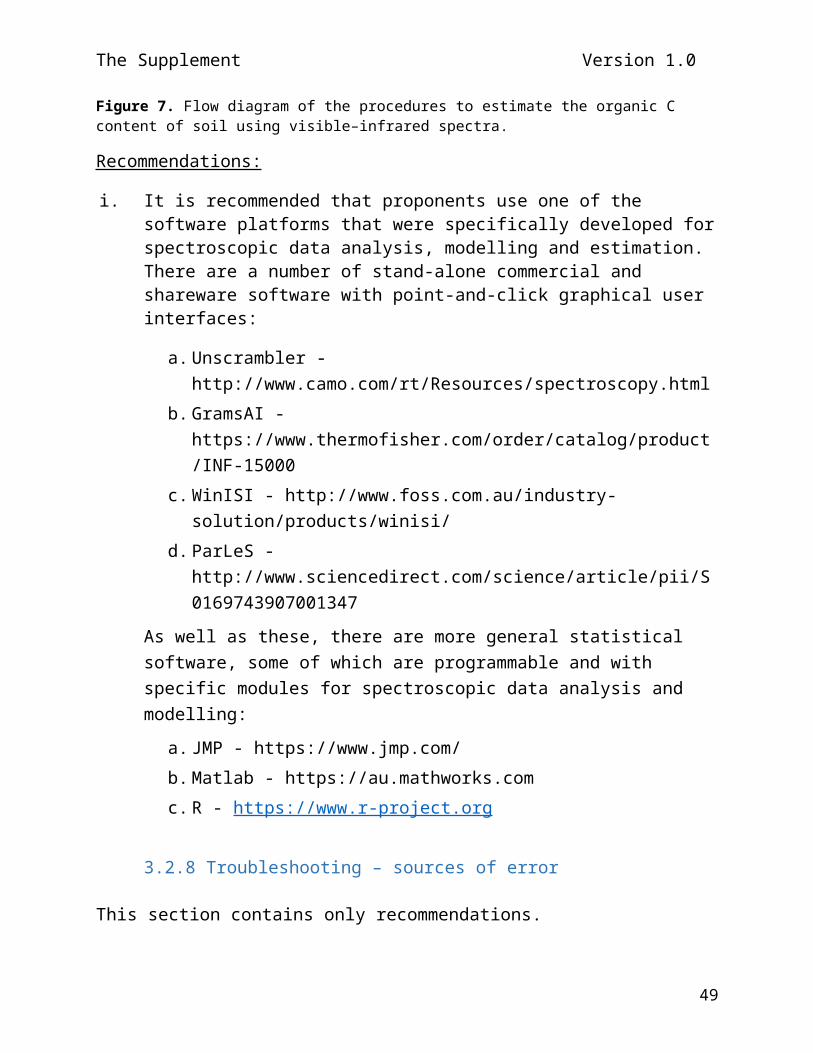
The Supplement Version 1.0
Winter 3.884 2.758 3.336 3.383 3.258 2.679 3.380
Kimberley Spring 3.853 2.491 2.706 3.132 2.859 2.244 2.462 Summer 5.488 2.117 4.176 2.798 5.311 1.883 2.201 Autumn 5.655 2.497 4.345 3.261 4.111 2.166 2.527 Winter 4.177 2.438 3.389 2.931 3.029 1.898 2.435
Table 3: Dairy Cattle (g) Emission Factors (kg CO2-e/head/day)State
(i)Class (j)
Milking Cows
Heifers >1
Heifers <1
Dairy Bulls >1
Dairy Bulls <1
NSW/ACT 11.493 4.333 2.112 5.389 2.592Northern Territory
11.251 4.412 2.151 5.487 2.640
Queensland 11.054 4.412 2.151 5.487 2.640South Australia 11.685 4.333 2.112 5.389 2.592
Tasmania 10.817 4.333 2.112 5.389 2.592Victoria 11.597 4.333 2.112 5.389 2.592Western Australia
12.048 4.333 2.112 5.389 2.592
Table 4: Other Livestock Emission Factors (kg CO2-e/head/day)State
(i)Species (g)
Goats Horses Deer Buffalo Donkeys /Mules
Emus/ Ostriches
Alpacas Camels
NSW/ACT 0.39 1.49 1.46 4.03 0.77 0.22 0.59 3.41
Northern Territory
0.40 1.55 1.48 4.08 0.79 0.23 0.60 3.47
Queensland 0.38 1.47 1.45 4.00 0.76 0.21 0.59 3.39
South Australia
0.39 1.50 1.46 4.04 0.78 0.22 0.60 3.42
Tasmania 0.40 1.57 1.48 4.10 0.80 0.23 0.61 3.49Victoria 0.40 1.54 1.47 4.08 0.79 0.23 0.60 3.46Western Australia
0.40 1.53 1.47 4.07 0.79 0.22 0.60 3.45
Table 5: Synthetic Fertiliser Emission Factors (t CO2-e/t Fertiliser N)Production System
(j)State (i)
NSW NT QLD SA TAS VIC WAIrrigated pasture 3.114 3.114 3.114 3.114 3.114 3.114 3.114
Irrigated crop 5.432 5.432 5.432 5.432 5.432 5.432 5.432
49
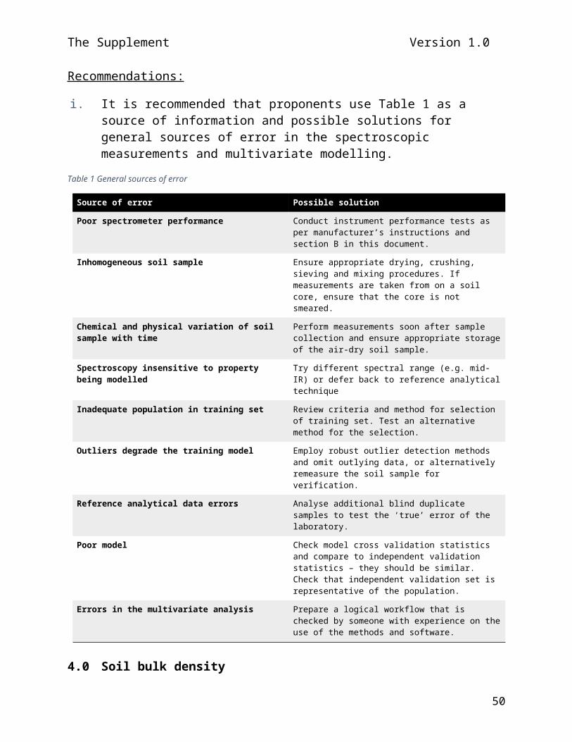
The Supplement Version 1.0
Non-irrigated pasture 1.382 1.885 1.165 1.776 2.074 1.931 1.565Non-irrigated crop 1.232 1.849 1.075 1.325 2.068 1.491 1.265
Sugar cane 11.293 NO 10.942 NO NO 10.251 11.051Cotton 3.092 NO 2.912 NO NO 2.833 3.633
Horticulture / vegetables 5.009 5.282 4.687 5.081 5.428 5.118 5.339
Table 6: Carbon dioxide emissions from urea applied as synthetic fertiliserProduction System
(j)Total emissions from synthetic fertiliser (t CO2-e/t urea)
ESF , B
Urea 0.7333
Table 7: Crop Residue ParametersCrop type (v) N content of residues Residue
emission factor
(t CO2-e/tN)
NC v, AB NCv,BG EFR
Wheat 0.00792 0.00383 4.68Barley 0.00764 0.00349 4.68Maize 0.00344 0.00188 4.68Oats 0.00750 0.00537 4.68Rice 0.00734 0.00168 4.68Sorghum 0.0096 0.00185 4.68Triticale 0.00792 0.00554 4.68Other Cereals 0.00771 0.00463 4.68Pulses 0.01073 0.00608 4.68Tuber and Roots 0.0017 0.00037 4.68Sugar cane 0.00125 0.00085 4.68Peanuts 0.01370 0.00240 4.68Cotton 0.0171 0.00513 4.68Hops 0.00792 NA 4.68Oilseeds 0.01797 0.00659 4.68Forage Crops 0.00708 0.00436 4.68
Table 8: Pasture Renewal Parameters
Dry Matter Yield
(t DM/ha) Nitrogen content of Residues
Residue emission factor
(t CO2-e/tN)
OP NCP , AB NCP,BG EFR
Grasses 7.1 0.0218 0.00872 4.68
Table 9: Agriculture lime application parameters
50

The Supplement Version 1.0
Emission factor(t C/t CaCO3 or
t CaMg(CO3)2
Dolomite 0.13Limestone 0.12
51

The Supplement Version 1.0
Part F: Additional Reporting RequirementsRequirements:
i. It is a requirement to include the following information in each offsets report that spectroscopy is used to analyse carbon content.
a. Spectrometer Manufacturer and model number Spectral range Instrument calibration material
b. Soil condition Measurement on intact cores – Y/N Measurement on homogenised soil (air dry/crushed /
ground/ sieved) – Y/Nc. Selection of training and validation data
Total number of spectra measured in the CEA Number of pairs of spectra and reference analytical
values selected in training set Method used for selection of training set Number of pairs of spectra and reference analytical
values selected for validation set Method used for selection of validation set Summary statistics for the training and validation sets
showing the mean, standard deviation, minimum, first quartile, median, third quartile, maximum, and skewness coefficient.
d. Reference analytical approach Reference analytical approach used Value for the SEL calculated on the ‘blind duplicate’
samples (if conducted)e. Spectroscopic modelling
If used, the methods used for spectral transformations, pre-processing and pre-treatment
If used, the method for correcting for the effects of water on the spectra
If used, the statistical transformation of the reference analytical data
The method used for the multivariate spectroscopic modelling
52

The Supplement Version 1.0
If any, the number of outliers removed, their analytical values and the outlier detection method used
The optimised settings for the spectroscopic model The model residuals plot The cross validation R2 and RMSE for the optimised
model, indicating whether the organic C data was transformed and which transformation was used.
f. Validation of the spectroscopic model Independent validation statistics R2, RMSE, SDE,
ME. Plot of the observed vs predicted values.
g. Estimates of unknowns – summary statistics for the estimates showing Mean Standard deviation Minimum First quartile Median Third quartile Maximum Skewness coefficient.
h. Software(s) used and version(s) number.i. Datasets
Total set of spectra collected along with the sample identification numbers, date and time of sampling, spatial location from which it was sourced (or locations, if it is a homogenised sample), depth layer (in cm).
Training set with sample identification numbers, soil organic C data and corresponding spectra
Validation set with sample identification numbers, soil organic C data and corresponding spectra
Prediction set with sample identification numbers, spectra and corresponding predictions of soil organic C
ii. It is a requirement to include the following information in each offsets report that gamma attenuation is used to determine bulk density.
a. Gamma-ray attenuation instrument used Manufacturer and model number Radiation source, activity (in MBq) and peak gamma
energy (in MeV) Type of scintillation detector and size
53

The Supplement Version 1.0
b. Soil condition and set up Measurements on soil cores at field condition or oven-
dried? A photograph of the instrument setup
c. Measurements Experimental values for s, and w. Values for parameters used to compute soil bulk
density in Equation (3) Method used for the independent measure of in
Equation (3). If spectroscopy, follow instructions in ‘The spectroscopic modelling procedure’ and the reporting requirements as above.
Number of measurements within the 0–30 cm, as well as where applicable, number of measurements within the 30–60 cm layer and the 60–100+ cm layer.
d. Datasets The instrument monitoring data recorded daily at the
start of the measurements, showing the counts per second attained for each of the standard materials with known densities as well as the densities of the known standards used.
All of the gamma and derived bulk density data collected along with the spatial location from which it was sourced.
54
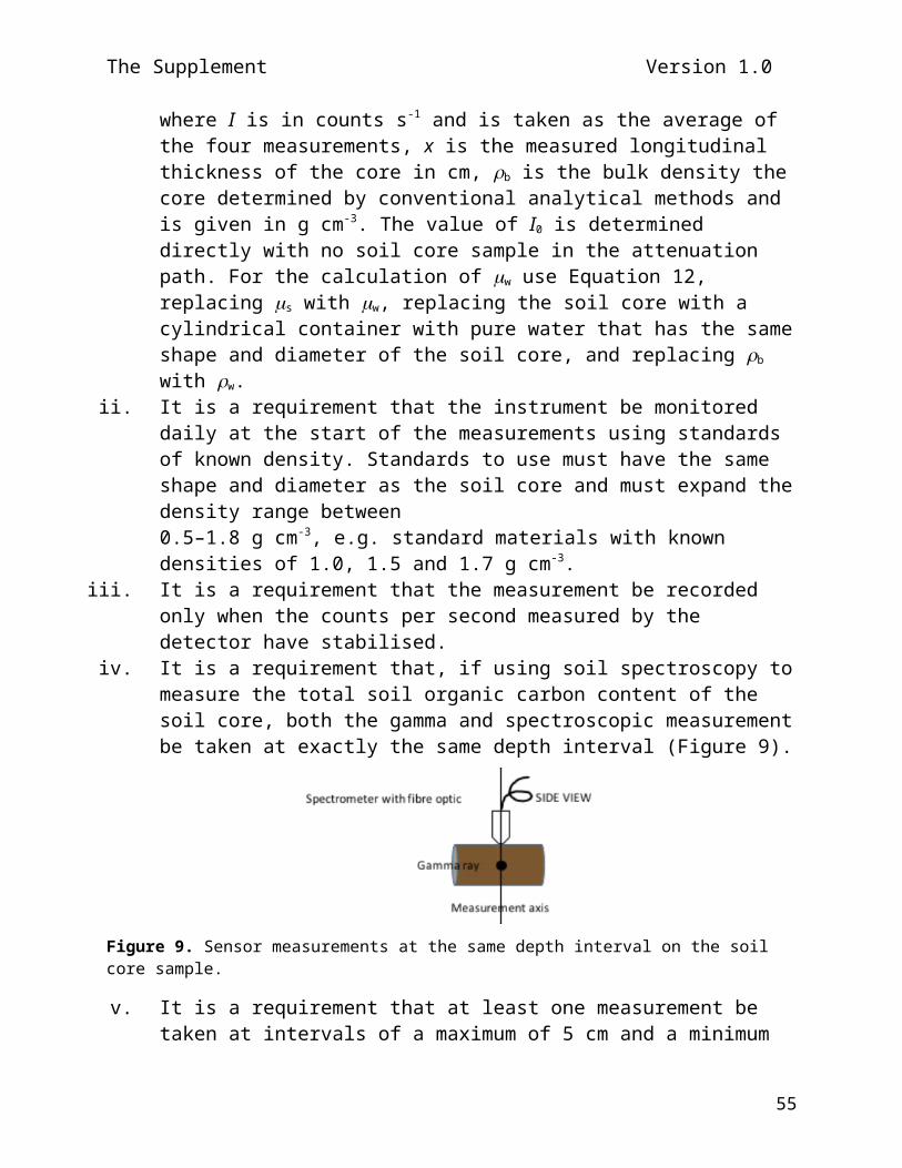
The Supplement Version 1.0
Part G: GlossaryAbsorption - absorption of radiation, as a function of frequency or wavelength, due to its interaction with the soil. Accuracy, precision and bias - accuracy (measured by the root mean squared error, RMSE) refers to how close a measured value is to the actual 'true’ value; precision (measured by the standard deviation of the error, SDE) is how close the measured values are to each other; and bias (measured by the mean error, ME) is a systematic error which makes all measurements wrong by a certain amount. RMSE2 = SDE2 + ME2. Equations for these statistic are:
RMSE=√∑i=1
N ( y i− y i)2
N ,
SDE=√∑i=1
N ( yi− y )2
(N−1),
ME=∑i=1
N ( y i− yi )N
,
where y i is the predicted value for sample i, y i is the observed value for sample i, y is the mean of the observed values, and N is the number of data.Air dry soil – soil that has been dried at approximately 40° C for 48 hours or until constant mass is achieved. It is advised to air dry at temperatures of around 40° C because temperatures above 65 ° C can activate carbon oxidation. Calibration - Operation that, under specified conditions, establishes a relation between the quantity values provided by measurement standards and corresponding spectrometer and uses this information to establish a relation for obtaining a measurement result from the spectrometer.Confidence limits – represent Confidence limits for the mean are an interval estimate for the mean. The interval estimate gives an indication of how much uncertainty there is in our estimate of the true mean. The narrower the interval, the more precise is our estimate. Confidence limits are defined as:
55

The Supplement Version 1.0
y ±t1−α
2 ,N−1
s√N
where y is the sample mean value of the organic C predictions, s is the samples standard deviation, N is the sample size, t 1−α
2, N−1 is the
value of the t-distribution with N–1 degrees of freedom for the desired for the desired probability level α. For a 95% confidence interval, α=0.05.Diffuse reflection - reflection of light from the soil surface such that an incident ray interacts with the soil and is reflected at many angles rather than at just one angle.Electromagnetic radiation – refers to the waves of the electromagnetic field, propagating through space carrying electromagnetic radiant energy e.g. visible and infrared radiation. It is commonly treated as a wave phenomenon, characterized by a wavelength or frequency.Estimate - the value of the component concentration or soil property obtained by applying the multivariate (spectroscopic) model.Frequency – defined as the number of crests of a wave of the electromagnetic radiation that move past a given point in a given unit of time. The most common unit of frequency is the hertz (Hz), corresponding to one crest per second. Typical units of frequency used in mid-IR spectroscopy are reciprocal centimetres or wave numbers (cm−1). Model validation - the process of testing a multivariate (spectroscopic) model to determine accuracy between the estimates from the model and the reference analytical method Multivariate (spectroscopic) modelling - a process for creating a model that relates component concentrations of soil properties to the absorbance of a set of know reference samples at more than one wavelength. Multivariate statistics - Multivariate statistics encompasses the simultaneous observation and analysis of more than one outcome variable. Prediction set – the set of soil samples with spectra but no other analytical data onto which the spectroscopic model is to be
56

The Supplement Version 1.0
generalised for predictions of the analyte.Reference analytical approach - the analytical method that is used to estimate the component concentration of the soil property value that is used in the modelling and validation procedures.Reference analytical values - the carbon concentrations for the training or validation sets that are measured using the reference analytical approach. Standard error of laboratory measurements (SEL) – represents the precision of a laboratory method. It can be determined can be determined by using one or more samples properly aliquoted and analysed in replicate by a laboratory. The average analytical value for the replicates on a single sample, x i, is determined by:
x i=∑j=1
r
xij
and the SEL is given by:
SEL=√∑i=1
N
∑j=1
M
(x ij−x i )2
N (r−1),
where x are the measurements on different samples, i, and different measurements, j, on the same sample, N are the total number of samples, M are the total number of measurements on the same sample, r, is the number of replicate analyses for each sample Standardised RMS, sRMSE – The sRMSE, shows the improvement that might be gained compared to using simply the mean of the training data as the prediction. Smaller values indicate less residual variance and better model validation. The sRMSE is calculated by:
sRMSE= RMSEy
where y is the mean of the observed values in the training set.Training set - the set of reference soil samples used for developing a multivariate (spectroscopic) model. These soil samples are analysed using a spectrometer and the reference analytical method.Validation set - the set of soil samples used in validating the multivariate (spectroscopic) model. The validation set are
57

The Supplement Version 1.0
independent of the training set, but also analysed using a spectrometer as well as the reference analytical method.Wavelength - defined as the distance between adjacent peaks (or troughs) in a wave of the electromagnetic radiation. Typically designated in units of meters, centimetres, micrometres (10-6 m) or nanometres (10-9 m).
58

The Supplement Version 1.0
Part H: ReferencesBarnes R J; Dhanoa M S; Lister S J 1989. ‘Standard normal variate transformation and de-trending of near-infrared diffuse reflectance spectra’. Applied Spectroscopy, 43(5), 772–777.Cook, R. Dennis; Weisberg, Sanford (1982). Residuals and Influence in Regression. (Repr. ed.). New York: Chapman and Hall. ISBN 041224280X.Cunningham,S; Roxburgh, S; Paul, K; Patti, A; Cavagnaro, T. 2017. ‘Generating spatially and statistically representative maps of environmental variables to test the efficiency of alternative sampling protocols’. Agriculture, Ecosystems and Environment, 243, pp103-113.De Gruijter JJ, McBratney AB, Minasny B, Wheeler I, Malone BP, Stockmann U. 2016. ‘Farm-scale soil carbon auditing’. Geoderma. 265: 120-130Fearn, T., 2001. ‘Standardisation and calibration transfer for near infrared instrument: a review’. Journal of Near Infrared Spectroscopy 9, 229–244.Geladi P; McDougel D; Martens H 1985. ‘Linearization and scatter correction for near infrared reflectance spectra of meat’. Application Spectroscopy, 39, 491–500.Ji, W., Viscarra Rossel, R. A., Shi, Z., 2015. ‘Accounting for the effects of water and the environment on proximally sensed vis–NIR soil spectra and their calibrations’. European Journal of Soil Science 66 (3), 555–565.Kalivas, JH and Gemperline, PJ 2006. Calibration. Chapter 5 in: Ed.P. Gemperline Practical guide to chemometrics. Second edition. Taylor & Francis Group, Boca Raton, Florida. Kennard, R.W. and Stone, L.A., 1969. ‘Computer aided design of experiments’. Technometrics, 11(1), pp.137–148.Lobsey, C., Viscarra Rossel RA. 2016. ‘Sensing soil bulk density for more accurate carbon accounting’. European Journal of Soil Science, 67(4): 504–513. Doi:10.1111/ejss.12355Martens H, Næs T, (1989) Multivariate calibration, John Wiley & Sons, Ltd, Chichester
59

The Supplement Version 1.0
Minasny, B., McBratney, A. B., Bellon-Maurel, V., Roger, J.-M., Gobrecht, A.,Ferrand, L., Joalland, S., 2011. ‘Removing the effect of soil moisture from NIR diffuse reflectance spectra for the prediction of soil organic carbon’. Geoderma 167–168,118–124.Orton, T; Pringle, M; Allen, D; Dalal, R; Bishop, T. 2015. ‘A geostatistical method to account for the number of aliquots in composite samples for normal and lognormal random variables’. European Journal of Soil Science. 66(6), pp.1023-1032.Pringle, M; Allen, D; Dalal, R; Payne, J; Mayer, D; O’Reagain, P; Marchant, B. 2011. ‘Soil carbon stock in the tropical rangelands of Australia: Effects of soil type and grazing pressure, and determination of sampling requirement’. Geoderma. 167-168. pp. 261-273.Savitzky, A., and Golay, M.J.E., 1964. ‘Smoothing and differentiation of data by simplified least squares procedures’. Anal. Chem. 36, 1627-1639.Shenk, J.S., and Westerhaus, M.O., 1991. ‘Population Definition, Sample Selection, and Calibration Procedures for Near Infrared Reflectance Spectroscopy'. Crop Science 31, 469-474.
Snee, R.D., 1977. ‘Validation of regression models: methods and examples’. Technometrics 19, 415-428.
Viscarra Rossel, RA. 2007. ‘Robust modelling of soil diffuse reflectance spectra by bagging-partial least squares regression’. Journal of Near Infrared Spectroscopy 15: 39–47.
Viscarra Rossel, RA, Behrens, T. 2010. Using data mining to model and interpret soil diffuse reflectance spectra. Geoderma 158: 46–54.
Viscarra Rossel RA, Behrens T, Ben-Dor E, Brown DJ, Dematte JAM, Shepherd KD, Shi Z, Stenberg B, Stevens A, Adamchuk VA., Aichi H, Barthes BG, Bartholomeus HM, Bayer AD, Bernoux M, Bottcher K,Brodsky L, Du CW, Chappell A, Fouad Y, Genot V, Gomez C, Grunwald S, Gubler A, Guerrero C, Hedley CB, Knadel M, Morras HJM, Nocita M, Ramirez-Lopez L, Roudier P, Rufasto Campos EM, Sanborn P, Sellitto VM, Sudduth KA, Rawlins BG, Walter C, Winowiecki LA, Hong SY, Ji W. 2016a.. ‘A global spectral library to characterize the world’s soil’. Earth-Science Reviews, 15: 198–230. dx.doi.org/10.1016/j.earscirev.2016.01.012
60

The Supplement Version 1.0
Viscarra Rossel RA, Brus DJ, Lobsey C, Shi Z, McLachlan G. 2016b. ‘Baseline estimates of soil organic carbon by proximal sensing: Comparing design-based, model-assisted and model-based inference’. Geoderma, 265: 152–163
61