The unification bonus (malus) in postwall Eastern Germany

1

The unification bonus (malus)in postwall Eastern Germany

Miriam Beblo*, Irwin L. Collier** and Thomas Knaus**

* Centre for European Economic Research, Mannheim (ZEW)** Freie Universität Berlin

February 2001

- Preliminary Version -- Please do not quote without permission of authors-

Abstract

We investigate the unification bonus as the discounted value of the differencebetween an Eastern German’s actual income and the counterfactual real incomestream that would have been experienced under a continuation of economic lifein a static GDR from 1990 to 1998. The two main issues tackled in this study arethe construction of valid deflators for a comparison of real incomes in transitionfrom a centralized to a market economy and the estimation of counterfactualincome streams. Our central result is that 19 percent of East Germans received apresent value malus and so can be regarded as unification losers.

Keywords: Real income comparison, income distribution and mobility,economies in transitionJEL code: D1, D3, P2

2

SummaryWe investigate the evolution and the distribution of the unification bonus ormalus for a representative sample of citizens of the former German DemocraticRepublic (GDR). The unification bonus is defined as the present discountedvalue as of July 1, 1990 of the difference between an Eastern Germanindividual’s actual real income stream (adjusted for household composition) andthe counterfactual real income stream that could have reasonably been expectedunder a continuation of economic life in a static GDR through 1998. Theassumption of a static GDR is both strong and optimistic, so our estimates of theproportion of economic losers from unification in the East can be regarded as anupper bound.

Two central issues are tackled in this study. First, the construction of validdeflators for a comparison of real incomes in transition from a centralized to amarket economy and second, the estimation of the hypothetical income streamsformer GDR citizens would have experienced under a continuation of the GDR.The deflators are calculated from a hitherto unexploited data set of the FederalStatistical Office (Statistisches Bundesamt). This data set also allows us tocalculate deflators for different points in the distribution of equivilized incomes.The hypothetical income streams are based on projections using the GermanSocio-Economic Panel that was expanded to include households from theGerman Democratic Republic in June 1990, hardly half a year after the Berlinwall had fallen and just before the wholesale introduction of the deutsche markto the East.

Our central result is that 19 percent of the East Germans are estimated to haveexperienced a present value malus from unification. Gains were sufficientlylarge that on average our sample experienced a cumulative bonus twice themagnitude of 1999 real income. We also find that the percentage of EastGermans with an annual unification malus is declining over time from 38percent in 1991 to 22 percent in 1998, however the rate of decline appears to belarger in the first part of the 1990s than in the second. This trend break fits wellwith the observed evolution of macroeconomic indicators for Eastern Germanyover the same time period.

Unlike any other transition economy, the elderly in the new federal states haveexperienced a dramatic improvement in their standards of living. Fewer than 2percent of East Germans above age 65 in 1990 had a negative bonus (i.e. amalus), whereas women between 45 and 54 show the highest proportion with amalus and women between 35 and 44 received the lowest net average bonus.

3

1 The problemOn the eve of German unification then Federal Chancellor Helmut Kohl madethe unambiguous claim that following German unification no one would beworse off and many would be much better off.1 A prediction that a genuinesocial and economic revolution will lead to a Pareto improvement in the strictsense of no losers whatsoever is hardly one based in human experience. Ourpurpose in this paper is to attempt to gauge the extent of the discrepancybetween Kohl’s verbalization of the hopes of many Germans during theeuphoria of just over one decade ago and the impressive, though definitelymixed, historical record that has unfolded in the meantime.

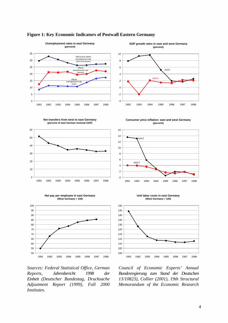
The six panels of Figure 1 capture much of the relevant aggregate story of EastGermany’s economic transition to the market economy. Simultaneous withsignificant real income gains, the East German labor market has beencharacterized by high and persistent unemployment rates. Official registeredunemployment does not include roughly half as many people again whoparticipate in active labor market programs (essentially income maintenanceschemes) or have accepted the terms of special early retirement pensions. TheGerman Council of Economic Experts counts these individuals – still nearly onemillion – as hidden unemployed. Hidden and registered unemployment togetherhas hovered at a level well above a quarter of the East German labor force forclose to a decade already. The initial strong recovery that followed theimmediate collapse of industrial production in the first year of economicunification2 was followed by a marked deceleration of real economic growth.Indeed, real GDP growth rates in East Germany have even fallen below those inWest Germany. The single most important difference between the East Germancase and all other economies in economic transition has of course been the goodfortune of a steady inflow of net transfers from West to East that continue andstill amount to approximately one third of the value of East German GDP eachyear. East Germans experienced a significant burst of inflation in the first yearsof unification and we note that nominal pay levels were indeed rapidly catchingup with West German levels. But as the final panel shows, productivity has notincreased nearly fast enough over the past decade to bring down East Germanunit labor costs in line with those in West Germany.

1 Less well remembered is that Helmut Kohl was most explicit in including both eastern andwestern Germany in his “promise”. The promise was made in Kohl’s speech on June 21,1990 before the Bundestag. It has been reprinted in Texte zur Deutschlandpolitik (1990),396.

2 Akerlof, et al. (1991).

4

Figure 1: Key Economic Indicators of Postwall Eastern Germany

Sources: Federal Statistical Office, German Council of Economic Experts’ AnnualReports, Jahresbericht 1998 der Bundesregierung zum Stand der DeutschenEinheit (Deutscher Bundestag, Drucksache 13/10823), Collier (2001), 19th StructuralAdjustment Report (1999), Fall 2000 Memorandum of the Economic ResearchInstitutes.

Unemployment rates in east Germany(percent)

Official plus hidden unemployment rate(men and women)

Official unemployment rate

(women)

Official unemployment rate

(men)

0

5

10

15

20

25

30

35

1991 1992 1993 1994 1995 1996 1997 1998

GDP growth rates in east and west Germany(percent)

EAST

WEST

-4

-2

0

2

4

6

8

10

1992 1993 1994 1995 1996 1997 1998

Net transfers from west to east Germany(percent of east German nominal GDP)

0

10

20

30

40

50

60

1991 1992 1993 1994 1995 1996 1997 1998

Consumer price inflation: east and west Germany(percent)

EAST

WEST

0

2

4

6

8

10

12

14

16

1991 1992 1993 1994 1995 1996 1997 1998

Net pay per employee in east Germany(West Germany = 100)

50

55

60

65

70

75

80

85

90

95

100

1991 1992 1993 1994 1995 1996 1997 1998

Unit labor costs in east Germany(West Germany = 100)

100

105

110

115

120

125

130

135

140

145

150

1991 1992 1993 1994 1995 1996 1997 1998

5

One striking pattern is immediately apparent in the panels of Figure 1: the mid-1990s reveal a break in the trend or even trend reversal. This pattern is also seenin our analysis that follows.

With the aggregate background brushed in with a few broad empirical strokes,we are ready to begin the detailed microeconometric examination of the courseof nominal incomes and prices. The object of our empirical attention is what wehave chosen to call the unification bonus defined as the present discounted valueas of July 1, 1990 of the difference between an Eastern German individual’sobserved real income stream (adjusted for household composition) and thecounterfactual real income stream that would have been experienced under acontinuation of economic life in a static GDR through 1998. For lack of a betterterm we call a negative bonus a unification malus. While there can be no doubtthat such a measure of economic welfare should be systematically related towhat is generally understood as the winners and losers from German unification,economic welfare is only one of several dimensions of social welfare. We hopethat careful readers will share our reluctance to leap from the distribution of theunification bonus or malus to the grand question of “winners” versus “losers”just quite yet.3 Still we believe the principal contribution of this paper is that itoffers the best estimates to date of the real income gains and losses in EasternGermany following the reunification of Germany in 1990.

Previous economic studies that have examined the impact of reunification at theindividual level have for the most part exclusively focussed on nominal incomemobility in East Germany. Among those Krause and Habich (1993) look at thechanges of household income that took place during the early years of transition,Hauser and Fabig (1999) investigate labor and household income mobilitybetween 1990 and 1995 and Steiner and Kraus (1996) analyze the distribution oflabor income from 1989 to 1993. All studies use the German Socio-EconomicPanel. The main results from these studies have been that income mobility in theEast was higher at first and has approached the Western level over time. Theprobability of falling within the distribution is higher for individuals andhouseholds who have experienced unemployment. Women are more at risk toend up in a lower income quantile than men. However due to the lack ofanything but extremely crude purchasing power parity indexes that link post-GDR prices in Eastern Germany to prices in the GDR, there are really nosatisfactory comparisons of 1990 real incomes with those in 1998.

3 Readers will also note that we often fail to take our own advice and in the interest ofexpository convenience will refer to winners and losers anyway. When we refer to winnerswe only mean a unification bonus greater than zero.

6

In his 1992 study Richard Hauser conjectured that inequality would increase inEastern Germany during the transition process. Indeed this hypothesis wasconfirmed in a later study by Hauser and Wagner (1996). Similarly Grabka andOtto (2001) calculate that East German market incomes have become moreunequally distributed over time. We are concerned in this paper with thedistribution of the unification bonus which we believe is a better indicator forwelfare gains from transition.

The lack of appropriate purchasing power parities to convert the 1990 EasternMark into DM is widely recognized throughout the literature. For exampleHauser (1992: 62) does point to the presence of quantity constraints and theextensive use of subsidies in the former GDR that make a satisfactorycomparison of the purchasing power of money in divided Germany difficult toachieve. Here is where the main contribution of the present paper is to be found:the combination of forecasts of GDR living standards, tailored to individual andhousehold circumstances, with purchasing-power-parity indexes that link post-GDR prices in Eastern Germany to prices in the GDR on the eve of Germaneconomic unification.

The household income data we analyze are also taken from the German Socio-Economic Panel (GSOEP) that began to include Eastern German households(1,944 individuals are in our sample) even before German Economic, Monetaryand Social Union actually went into effect on July 1, 1990. Exact price deflatorshave been constructed from data collected by the German Federal StatisticalOffice. The assumption of a static GDR economy as the benchmark for ourcounterfactual has been chosen more for the psychological salience of the finalyear of the GDR economy than as a realistic forecast of an economy whose timewas indeed running out4. This is probably the best reason to consider ourestimate of the aggregate unification bonus as merely a lower bound for the truebonus. The assumption of static expectations has the additional merit ofproviding a way to use the cross-section of economic life reported in the firstEastern wave of GSOEP to generate counterfactual real income streams to thepresent, conditional on individual characteristics. The assumption of staticexpectations excludes economic growth or equivalently any cohort effects. Wehave assumed that as an individual’s age, household composition and job-relatedcharacteristics changed over the past decade, the relevant comparison forjudging his or her relative gain or loss would be that of someone else with thesame age and other individual characteristics in the 1990 sample. We calculate

4 This is the more or less the bottom line of the classified report prepared for the GDR’sPolitbüro dated October 30, 1989 prepared by the Chairman of the State PlanningCommission, see Schürer (1992).

7

the unification bonus from the perspective of the individual and not thehousehold.

According to our estimates for about 19 percent of the GSOEP sample ages 25years and above at the time of German unification, real income losses followingGerman economic unification have actually exceeded the gains. On the otherhand, we also calculate that aggregate gains of the unification winners haveswamped the aggregate losses of the losers. Expressed as a present discountedvalue (valued in 1991 DM) the average bonus of the 81% unification winnerswas over 39,000 DM vs. the average unification loss of 15,700 DM of the other19% of our sample. The vast bulk of the unification malus has been concentratedin the cohorts that were between 35 and 54 years of age in 1990 with the largestunification bonuses going to those 55 years and older in 1990.

One disturbing tendency observed in our data is that figures for 1997 and 1998point to a falling share of those with a positive annual unification gain, adevelopment that is hardly surprising in light of the dramatic deceleration thatoccurred in Eastern German GDP growth during the second half of the 1990s. Atentative eyeball-interpretation is that we could indeed be seeing a trend reversalthat is obscured by limiting one’s attention to the single summary present-valuebonus.

Two central issues are tackled in sections 2 and 3: first, the construction of pricedeflators needed to convert nominal magnitudes into their corresponding realcounterparts; second, the estimation of the counterfactual income streams thateast Germans could have reasonably expected under a static continuation of theGDR into the late 1990s. In sections 4 and 5 we combine observations, deflatorsand counterfactuals to produce our empirical results. Given the necessarilytentative nature of such calculations, we conclude our paper with a summarythat helps to identify certain structural weaknesses of our estimates that naturallyconstitute an agenda for future research.

2 Getting real: deflatorsThe first order of business is the conversion of the GSOEP 1990 East Germanincome data (valued in GDR marks) into meaningful DM magnitudes. Indexesof relative purchasing power used in a comparison involving two very differenteconomic systems need to adjust for differences in the extent of nonpricerationing (i.e. quantity constraints) as well as for differences in the indirecttaxation/subsidization of consumer goods, see Collier (1986 and 1989). This isparticularly true when one considers the enormous differences between the Eastand West housing markets and the degree of subsidization with respect to basicfoodstuffs and children’s clothing (in the East) in pre-unification Germany. Theestimates of real household net income used for this paper are based upon

8

purchasing power parities that provide at least partial correction for thedistortion of quantity constraints and the differential impact of indirecttaxes/subsidies across the GDR income distribution. In this section we providethe interested reader a brief description of the methodology used to calculateexact price deflators.5

The key hypothesis behind the price deflators is that West and East Germans areassumed to have had and still have identical preferences. This is completelywithin the spirit of conventional applied demand analysis, some would evenargue it is the hallmark of economic analysis as opposed to sociological oranthropological analysis. The difficult of part of applying the tools of empiricaldemand analysis to our problem is that these methods have evolved over thedecades in the analysis of household budgets in market economies for whichquantity constraints are a pathological exception rather than the rule. Certainlyfor our GDR observations and at least in the initial years following Germaneconomic unification, both budget and quantity constraints are an essential partof the story.

This complication means that the presumption of the tangency of budgetconstraints and indifference surfaces (a necessary condition for utilitymaximization for households that are solely budget constrained in theirexpenditure choices) is wholly inappropriate in an economic world of quantityconstraints. For this reason it would be invalid to use observed Eastern budgetsand quantity data to infer the parameters of the underlying preferences ofhouseholds without detailed information on the extent and incidence of quantityconstraints. One way out of this apparent dead-end is to exploit the existence ofthe fraternal twin Germany, i.e. the old FRG, to estimate “all-Germanpreferences” from observed budgets and market baskets in West Germany andto transplant the estimated demand system eastwards for the purpose ofinterpreting the structure of household expenditure observed there.

The West German expenditure data6 are available according to a consistentclassification system for the period 1981-1998. Demand systems wereestimated using annual average expenditures for (i) two-adult households(predominantly elderly) whose principal source of income is public pensionsand/or public assistance and (ii) two-parent, two children households that aredisaggregated into middle-income and higher-income groups. The consumerprice indexes for the sixteen categories of expenditure in West Germany have

5 The deflators used to convert nominal equivalent incomes into DM at 1991 West Germanprices are taken from Collier (2001) to which the reader is referred for a full description ofboth data and methods.

6 Statistisches Bundesamt Fachserie 15. Reihe 1. (1984-1998).

9

been assembled for the most part by a straight-forward chaining of thecorresponding indexes7 for base years 1980, 1985, 1991 and 1995. All categoryprice indexes have been set equal to unity for 1991.8

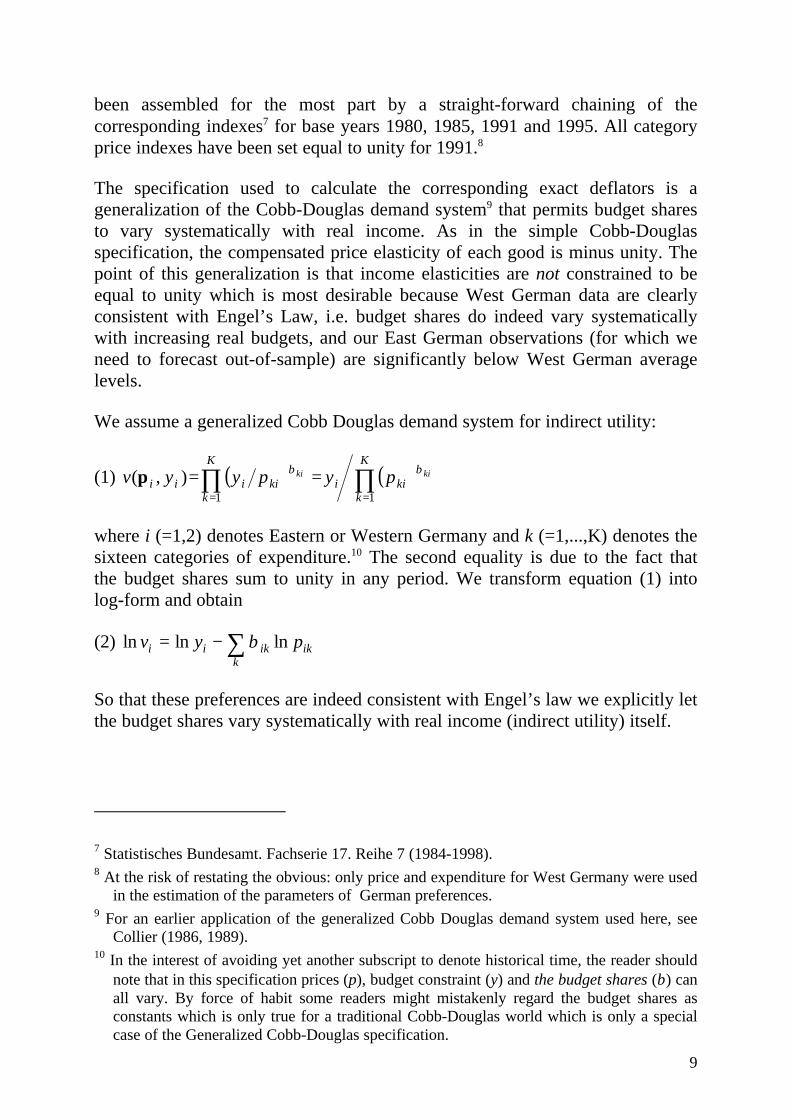
The specification used to calculate the corresponding exact deflators is ageneralization of the Cobb-Douglas demand system9 that permits budget sharesto vary systematically with real income. As in the simple Cobb-Douglasspecification, the compensated price elasticity of each good is minus unity. Thepoint of this generalization is that income elasticities are not constrained to beequal to unity which is most desirable because West German data are clearlyconsistent with Engel’s Law, i.e. budget shares do indeed vary systematicallywith increasing real budgets, and our East German observations (for which weneed to forecast out-of-sample) are significantly below West German averagelevels.

We assume a generalized Cobb Douglas demand system for indirect utility:

(1) ( ) ( )∏∏==

==K

kkii

K

kkiiii

kiki pypyyv11

),( ββp

where i (=1,2) denotes Eastern or Western Germany and k (=1,...,K) denotes thesixteen categories of expenditure.10 The second equality is due to the fact thatthe budget shares sum to unity in any period. We transform equation (1) intolog-form and obtain

(2) ∑−=k

ikikii pyv lnlnln β

So that these preferences are indeed consistent with Engel’s law we explicitly letthe budget shares vary systematically with real income (indirect utility) itself.

7 Statistisches Bundesamt. Fachserie 17. Reihe 7 (1984-1998).8 At the risk of restating the obvious: only price and expenditure for West Germany were used

in the estimation of the parameters of German preferences.9 For an earlier application of the generalized Cobb Douglas demand system used here, see

Collier (1986, 1989).10 In the interest of avoiding yet another subscript to denote historical time, the reader should

note that in this specification prices (p), budget constraint (y) and the budget shares (β) canall vary. By force of habit some readers might mistakenly regard the budget shares asconstants which is only true for a traditional Cobb-Douglas world which is only a specialcase of the Generalized Cobb-Douglas specification.

10

(3)

∑=

=K

mim

ikki

m

k

v

v

1

γ

γ

α

αβ

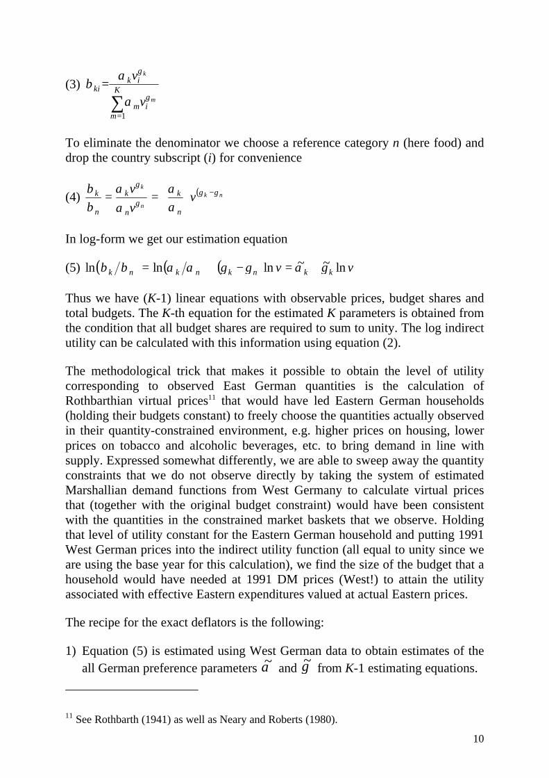
To eliminate the denominator we choose a reference category n (here food) anddrop the country subscript (i) for convenience

(4) ( )nk

n

k

vv

v

n

k

n

k

n

k γγγ

γ

αα

αα

ββ −

==

In log-form we get our estimation equation

(5) ( ) ( ) ( ) vv kknknknk ln~~lnlnln γαγγααββ +=−+=

Thus we have (K-1) linear equations with observable prices, budget shares andtotal budgets. The K-th equation for the estimated K parameters is obtained fromthe condition that all budget shares are required to sum to unity. The log indirectutility can be calculated with this information using equation (2).

The methodological trick that makes it possible to obtain the level of utilitycorresponding to observed East German quantities is the calculation ofRothbarthian virtual prices11 that would have led Eastern German households(holding their budgets constant) to freely choose the quantities actually observedin their quantity-constrained environment, e.g. higher prices on housing, lowerprices on tobacco and alcoholic beverages, etc. to bring demand in line withsupply. Expressed somewhat differently, we are able to sweep away the quantityconstraints that we do not observe directly by taking the system of estimatedMarshallian demand functions from West Germany to calculate virtual pricesthat (together with the original budget constraint) would have been consistentwith the quantities in the constrained market baskets that we observe. Holdingthat level of utility constant for the Eastern German household and putting 1991West German prices into the indirect utility function (all equal to unity since weare using the base year for this calculation), we find the size of the budget that ahousehold would have needed at 1991 DM prices (West!) to attain the utilityassociated with effective Eastern expenditures valued at actual Eastern prices.

The recipe for the exact deflators is the following:

1) Equation (5) is estimated using West German data to obtain estimates of theall German preference parameters α~ and γ~ from K-1 estimating equations.

11 See Rothbarth (1941) as well as Neary and Roberts (1980).

11

2) Using the preference parameters estimated in step 1) and holding theobserved East German budget constraint constant, the level of the indirectutility function and the virtual prices associated with the observed quantitiesare simultaneously calculated.

3) Using the level of East German utility just calculated, we can calculated theDM expenditure total that would have been necessary to attain that level ofutility at 1991 West German prices.

4) The deflator is obtained by dividing the observed East German expenditureby the 1991-DM expenditure from step 3). The deflator has thedimensionality of Eastern marks per DM (1991 prices).

The original Eastern German family budget surveys for 1989 as well as the firstand second halves of 1990 were re-aggregated to conform to the WesternGerman classification system by team working for the Federal StatisticalOffice12 and fully comparable family budget surveys in East and West have beenconducted since 1991. Thus the time series of annual average family budgets forEastern and Western Germany for retired two adult households and middle-income/ high-income four person (two adults/two children) households arereasonably consistent both across time and space.

To obtain the consumer price indexes for Eastern Germany at the sixteencategory level used here, it was necessary to combine a bridge between the Eastand West German price levels from the second half on 199313 with chainedindexes for the Eastern German category price levels14. In other words, categoryby category direct price comparisons between East and West for one point intime have been backcast to 1989 and forward to 1998. When an Eastern Germanconsumer price index computed this way has a value of unity, then the EasternGerman price level for that category of expenditure and that year was equal tothe West German price level in 1991. The Eastern German price level for theconsumption expenditure categories “food” and “rent” have remained below thecorresponding West German price levels for those categories 1991 for the entireperiod under consideration.

12 Statistisches Bundesamt (1993a).13 The survey is described in Ströhl (1994). Mr. Ströhl graciously provided disaggregated data

that made the East/West price bridges for our sixteen categories possible.14 For May, June, July, December 1990 [ base 1989=100]: Statistisches Bundesamt (1992a:

15-19, 23-27, 63-67). For July 1990, December 1990 [base July 1990-June1991=100]:Statistisches Bundesamt (1992b). 1991 indexes [ base July 1990-June1991=100]:Statistisches Bundesamt Fachserie 17. Reihe 7. (1993: 234-262). 1991-1998 taken fromunpublished series made available by the Federal Statistical Office.

12

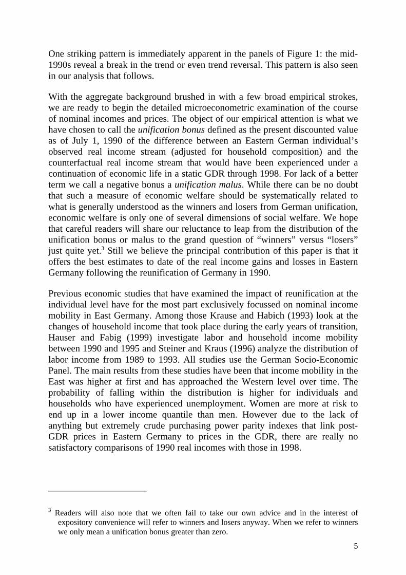
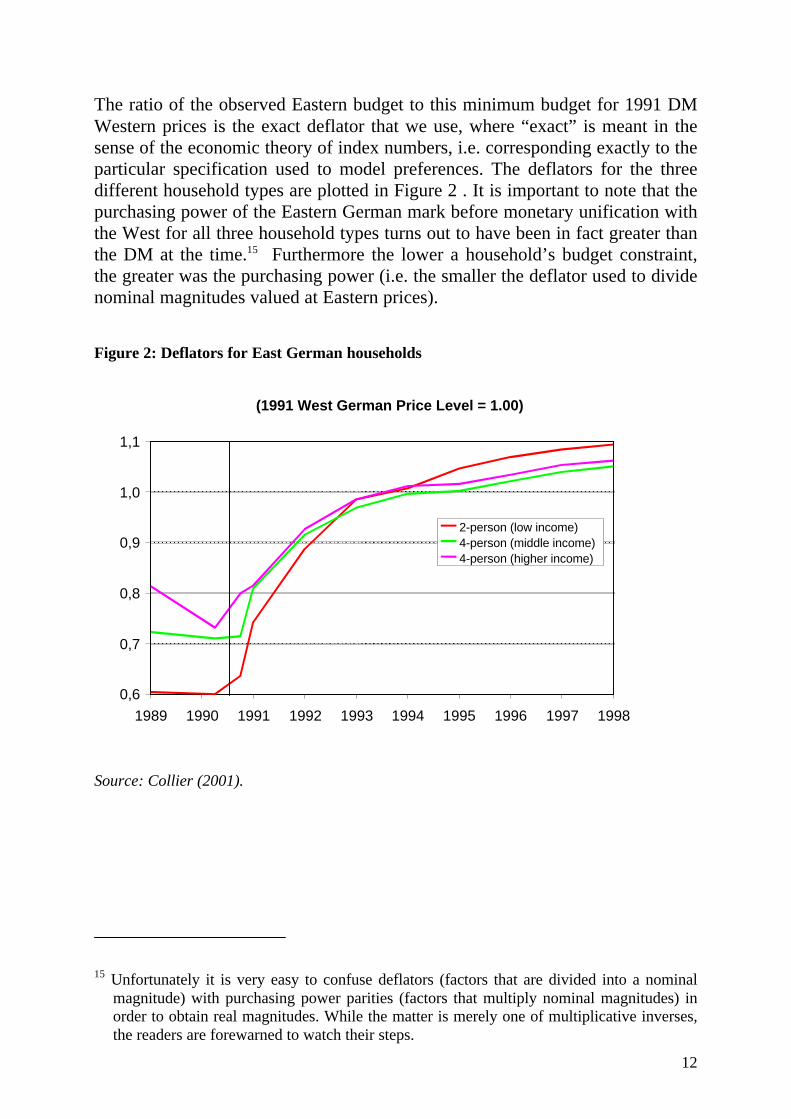
The ratio of the observed Eastern budget to this minimum budget for 1991 DMWestern prices is the exact deflator that we use, where “exact” is meant in thesense of the economic theory of index numbers, i.e. corresponding exactly to theparticular specification used to model preferences. The deflators for the threedifferent household types are plotted in Figure 2 . It is important to note that thepurchasing power of the Eastern German mark before monetary unification withthe West for all three household types turns out to have been in fact greater thanthe DM at the time.15 Furthermore the lower a household’s budget constraint,the greater was the purchasing power (i.e. the smaller the deflator used to dividenominal magnitudes valued at Eastern prices).

Figure 2: Deflators for East German households

(1991 West German Price Level = 1.00)

0,6

0,7

0,8

0,9

1,0

1,1

1989 1990 1991 1992 1993 1994 1995 1996 1997 1998

2-person (low income)4-person (middle income)4-person (higher income)

Source: Collier (2001).

15 Unfortunately it is very easy to confuse deflators (factors that are divided into a nominalmagnitude) with purchasing power parities (factors that multiply nominal magnitudes) inorder to obtain real magnitudes. While the matter is merely one of multiplicative inverses,the readers are forewarned to watch their steps.

13

3 Back in the GDRFor the purpose of establishing a baseline level of real disposable income, weare extremely fortunate to have the extraordinary data from the German Socio-Economic Panel (GSOEP)16. As an individual household micro-data panel, theGSOEP is a rich data source for analyzing income dynamics in relation withvarious individual and household characteristics. The GSOEP survey began in1984 in the Federal Republic of Germany (FRG). The GSOEP was expanded toinclude households from the German Democratic Republic (GDR) in June 1990,hardly half a year after the Berlin wall had fallen and just before monetary uniontook place. The empirical results presented in this section are based on that 1990sample representing the Germans residing in the GDR at the time of thesurvey.17

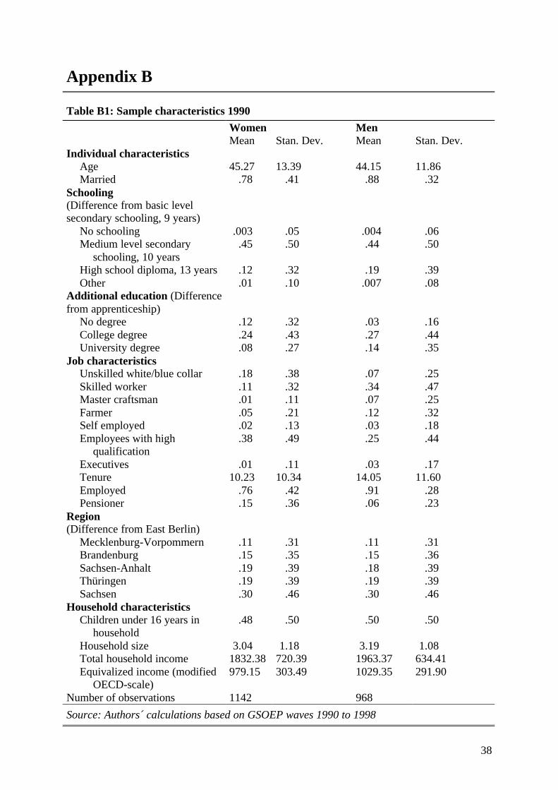
Further sample selection criteria are listed in Table 1. Our analysis covers allGDR respondents who participated in the survey in 1990 (before July) andremained in the panel in each subsequent year through 1998. It contains onlyGerman nationals. We have further restricted our sample to respondents 25 yearsand older at the time of unification in order to include only individuals whoalready had completed their education at the time of German unification so thatour results should not be affected by postwall educational decisions. Thus wehave excluded the youngest adult cohorts to avoid the considerable complicationentailed in valuing the returns to education. Observations with missing data forincome or any of the explanatory variables have also been dropped. The sampleused for income estimation consists of 2110 men and women ages 25 to 85.Descriptive statistics of the sample are provided in Table B1 of Appendix B.The average age of the sample selected is 45 for women and 44 for men. Thefinal sample used for the projection of counterfactual income streams through1998 comprises 1944 men and women.

16 For more information on the GSOEP see Wagner/Burkhauser/Behringer (1993) andProjektgruppe Sozio-oekonomisches Panel (1995).

17 A small fraction of interviews were conducted after monetary union went into effect onJuly 1, 1990. We have only included respondents who participated in the panel before thatdate so that all income variables from 1990 are expressed in GDR marks.

14

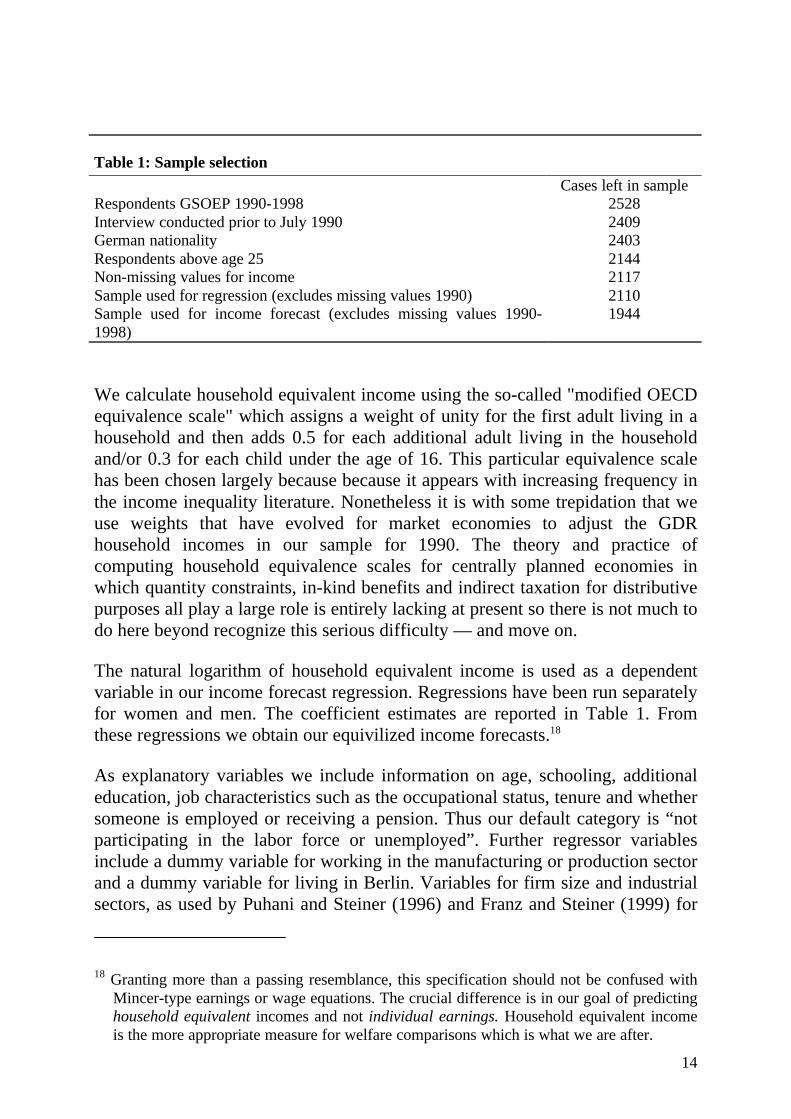
Table 1: Sample selectionCases left in sample

Respondents GSOEP 1990-1998 2528Interview conducted prior to July 1990 2409German nationality 2403Respondents above age 25 2144Non-missing values for income 2117Sample used for regression (excludes missing values 1990) 2110Sample used for income forecast (excludes missing values 1990-1998)

1944

We calculate household equivalent income using the so-called "modified OECDequivalence scale" which assigns a weight of unity for the first adult living in ahousehold and then adds 0.5 for each additional adult living in the householdand/or 0.3 for each child under the age of 16. This particular equivalence scalehas been chosen largely because because it appears with increasing frequency inthe income inequality literature. Nonetheless it is with some trepidation that weuse weights that have evolved for market economies to adjust the GDRhousehold incomes in our sample for 1990. The theory and practice ofcomputing household equivalence scales for centrally planned economies inwhich quantity constraints, in-kind benefits and indirect taxation for distributivepurposes all play a large role is entirely lacking at present so there is not much todo here beyond recognize this serious difficulty — and move on.

The natural logarithm of household equivalent income is used as a dependentvariable in our income forecast regression. Regressions have been run separatelyfor women and men. The coefficient estimates are reported in Table 1. Fromthese regressions we obtain our equivilized income forecasts.18

As explanatory variables we include information on age, schooling, additionaleducation, job characteristics such as the occupational status, tenure and whethersomeone is employed or receiving a pension. Thus our default category is “notparticipating in the labor force or unemployed”. Further regressor variablesinclude a dummy variable for working in the manufacturing or production sectorand a dummy variable for living in Berlin. Variables for firm size and industrialsectors, as used by Puhani and Steiner (1996) and Franz and Steiner (1999) for

18 Granting more than a passing resemblance, this specification should not be confused withMincer-type earnings or wage equations. The crucial difference is in our goal of predictinghousehold equivalent incomes and not individual earnings. Household equivalent incomeis the more appropriate measure for welfare comparisons which is what we are after.

15

explaining East German wages, were not found significantly related tohousehold equivalent income and are therefore not included in the estimationequation presented here.

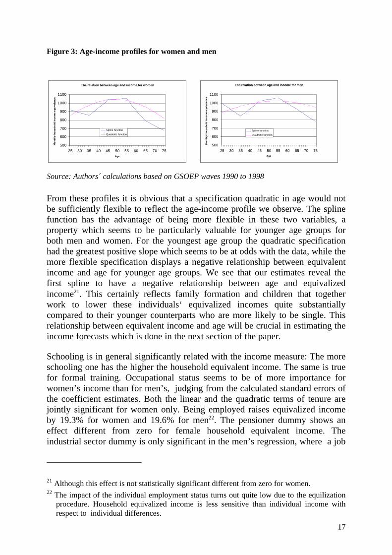
One of the most important explanatory variables for predicting future income isthe individual’s age. The shape of the age-income profile however stronglydepends on the assumed underlying functional form of the relationship betweenage and equivalence income. By using a spline function one can better allow fornon-linearities in this relationship while retaining a simple specification.19 Wehave chosen a specification using a linear spline function with five differentlinear splines, corresponding to five age groups (25-34, 35-44, 45-54, 55-64, 65years of age and older).

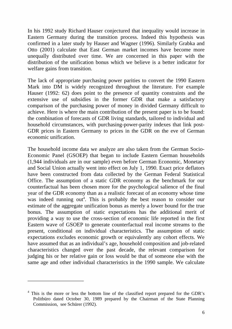
In Figure 3 we can see the resulting age-income locus for the spline functionthus specified. For the purpose of comparison, a different age-incomespecification using a linear plus a quadratic age term, is also shown.20

19 Linear splines capture the relationship between two variables as a piecewise linear function,in other words a function composed of linear segments joined at knots.

20 Both curves belong to the profile of a person who worked as a skilled employee, havingzero years of tenure and who falls into each of the reference categories used in theestimation equation for all remaining variables.

16

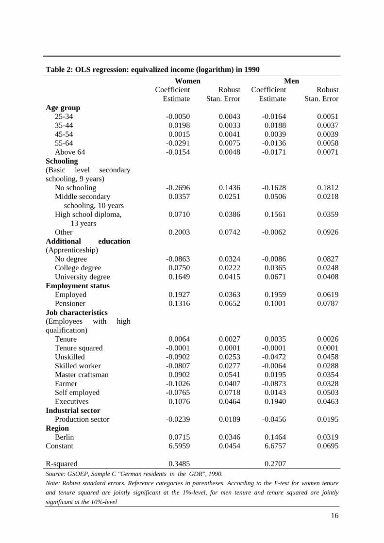
Table 2: OLS regression: equivalized income (logarithm) in 1990

Women MenCoefficient

EstimateRobust

Stan. ErrorCoefficient

EstimateRobust

Stan. ErrorAge group

25-34 -0.0050 0.0043 -0.0164 0.005135-44 0.0198 0.0033 0.0188 0.003745-54 0.0015 0.0041 0.0039 0.003955-64 -0.0291 0.0075 -0.0136 0.0058Above 64 -0.0154 0.0048 -0.0171 0.0071

Schooling(Basic level secondaryschooling, 9 years)

No schooling -0.2696 0.1436 -0.1628 0.1812Middle secondary

schooling, 10 years0.0357 0.0251 0.0506 0.0218

High school diploma, 13 years

0.0710 0.0386 0.1561 0.0359

Other 0.2003 0.0742 -0.0062 0.0926Additional education(Apprenticeship)

No degree -0.0863 0.0324 -0.0086 0.0827College degree 0.0750 0.0222 0.0365 0.0248University degree 0.1649 0.0415 0.0671 0.0408

Employment statusEmployed 0.1927 0.0363 0.1959 0.0619Pensioner 0.1316 0.0652 0.1001 0.0787

Job characteristics(Employees with highqualification)

Tenure 0.0064 0.0027 0.0035 0.0026Tenure squared -0.0001 0.0001 -0.0001 0.0001Unskilled -0.0902 0.0253 -0.0472 0.0458Skilled worker -0.0807 0.0277 -0.0064 0.0288Master craftsman 0.0902 0.0541 0.0195 0.0354Farmer -0.1026 0.0407 -0.0873 0.0328Self employed -0.0765 0.0718 0.0143 0.0503Executives 0.1076 0.0464 0.1940 0.0463

Industrial sectorProduction sector -0.0239 0.0189 -0.0456 0.0195

RegionBerlin 0.0715 0.0346 0.1464 0.0319

Constant 6.5959 0.0454 6.6757 0.0695

R-squared 0.3485 0.2707Source: GSOEP, Sample C "German residents in the GDR", 1990.

Note: Robust standard errors. Reference categories in parentheses. According to the F-test for women tenure

and tenure squared are jointly significant at the 1%-level, for men tenure and tenure squared are jointly

significant at the 10%-level

17

Figure 3: Age-income profiles for women and men

Source: Authors´ calculations based on GSOEP waves 1990 to 1998

From these profiles it is obvious that a specification quadratic in age would notbe sufficiently flexible to reflect the age-income profile we observe. The splinefunction has the advantage of being more flexible in these two variables, aproperty which seems to be particularly valuable for younger age groups forboth men and women. For the youngest age group the quadratic specificationhad the greatest positive slope which seems to be at odds with the data, while themore flexible specification displays a negative relationship between equivalentincome and age for younger age groups. We see that our estimates reveal thefirst spline to have a negative relationship between age and equivalizedincome21. This certainly reflects family formation and children that togetherwork to lower these individuals‘ equivalized incomes quite substantiallycompared to their younger counterparts who are more likely to be single. Thisrelationship between equivalent income and age will be crucial in estimating theincome forecasts which is done in the next section of the paper.

Schooling is in general significantly related with the income measure: The moreschooling one has the higher the household equivalent income. The same is truefor formal training. Occupational status seems to be of more importance forwomen’s income than for men’s, judging from the calculated standard errors ofthe coefficient estimates. Both the linear and the quadratic terms of tenure arejointly significant for women only. Being employed raises equivalized incomeby 19.3% for women and 19.6% for men22. The pensioner dummy shows aneffect different from zero for female household equivalent income. Theindustrial sector dummy is only significant in the men’s regression, where a job

21 Although this effect is not statistically significant different from zero for women.22 The impact of the individual employment status turns out quite low due to the equilization

procedure. Household equivalized income is less sensitive than individual income withrespect to individual differences.

The relation between age and income for women

500

600

700

800

900

1000

1100

25 30 35 40 45 50 55 60 65 70 75Age

Mo

nth

ly h

ou

seh

old

inco

me

equ

ival

ence

Spline function

Quadratic function

The relation between age and income for men

500

600

700

800

900

1000

1100

25 30 35 40 45 50 55 60 65 70 75Age

Mo

nth

ly h

ou

seh

old

inco

me

equ

ival

ence

Spline function

Quadratic function

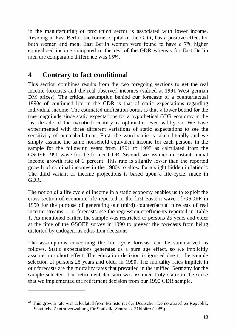
18

in the manufacturing or production sector is associated with lower income.Residing in East Berlin, the former capital of the GDR, has a positive effect forboth women and men. East Berlin women were found to have a 7% higherequivalized income compared to the rest of the GDR whereas for East Berlinmen the comparable difference was 15%.

4 Contrary to fact conditionalThis section combines results from the two foregoing sections to get the realincome forecasts and the real observed incomes (valued at 1991 West germanDM prices). The critical assumption behind our forecasts of a counterfactual1990s of continued life in the GDR is that of static expectations regardingindividual income. The estimated unification bonus is thus a lower bound for thetrue magnitude since static expectations for a hypothetical GDR economy in thelast decade of the twentieth century is optimistic, even wildly so. We haveexperimented with three different variations of static expectations to see thesensitivity of our calculations. First, the word static is taken literally and wesimply assume the same household equivalent income for each persons in thesample for the following years from 1991 to 1998 as calculated from theGSOEP 1990 wave for the former GDR. Second, we assume a constant annualincome growth rate of 3 percent. This rate is slightly lower than the reportedgrowth of nominal incomes in the 1980s to allow for a slight hidden inflation23.The third variant of income projections is based upon a life-cycle, made inGDR.

The notion of a life cycle of income in a static economy enables us to exploit thecross section of economic life reported in the first Eastern wave of GSOEP in1990 for the purpose of generating our (third) counterfactual forecasts of realincome streams. Our forecasts use the regression coefficients reported in Table1. As mentioned earlier, the sample was restricted to persons 25 years and olderat the time of the GSOEP survey in 1990 to prevent the forecasts from beingdistorted by endogenous education decisions.

The assumptions concerning the life cycle forecast can be summarized asfollows. Static expectations generates us a pure age effect, so we implicitlyassume no cohort effect. The education decision is ignored due to the sampleselection of persons 25 years and older in 1990. The mortality rates implicit inour forecasts are the mortality rates that prevailed in the unified Germany for thesample selected. The retirement decision was assumed truly static in the sensethat we implemented the retirement decision from our 1990 GDR sample.

23 This growth rate was calculated from Ministerrat der Deutschen Demokratischen Republik,Staatliche Zentralverwaltung für Statistik, Zentrales Zählbüro (1989).

19

For projection purposes we can distinguish between time-variant and time-invariant variables. The former capture the basic idea of a life cycle that can beestimated from a cross-section. From these cross-section estimates we forecastfuture incomes by assuming that the latter variables do not change over the lifecycle and the former variables by definition would change. The only time-variant variables in this sense are age, a variable that increments by one fromyear to year, and job-related characteristics. As soon as a woman (man) reachesthe pension age of 60 (65), both the participation and job-related dummies areset to zero and the pension dummy is set to unity. These ages are the modal1990 East German pension age for women and men. A detailed description anddocumentation of the procedure for obtaining income forecasts is provided inappendix A.

These forecast incomes are valued in 1990 East German marks as suits thecounterfactual of a frozen GDR. They are transformed by using the deflatorsfrom Section 2 above. Also the observed equivilized incomes are likewisetransformed into 1991 German marks using deflators calculated for each year.The differences between observed and forecast real equivilized monthly incomeare the annual unification bonuses (if positive) or maluses (if negative).

5 Evolution and distribution of the unification bonus(malus)

One of the central empirical results of this paper is the summary statistic that theproportion of East Germans with a present value unification malus through 1998was 19 percent, using a five percent real annual interest rate for discounting.This result, as all following, is based on the weighted income projection with thesample weights accounting for selection into the sample in 1990 and selection ofstaying in the panel until 1998. These calculations assume a individualperspective and not a household perspective and the persons are at least 25 yearsold in 1990.

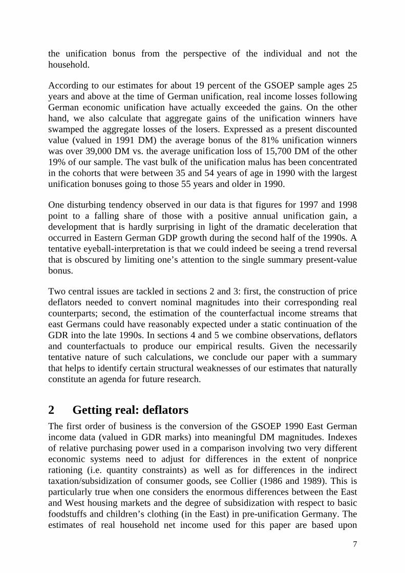
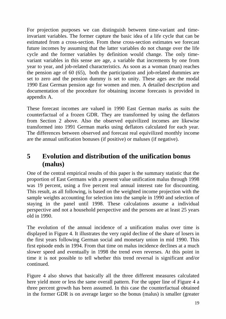
The evolution of the annual incidence of a unification malus over time isdisplayed in Figure 4. It illustrates the very rapid decline of the share of losers inthe first years following German social and monetary union in mid 1990. Thisfirst episode ends in 1994. From that time on malus incidence declines at a muchslower speed and eventually in 1998 the trend even reverses. At this point intime it is not possible to tell whether this trend reversal is significant and/orcontinued.

Figure 4 also shows that basically all the three different measures calculatedhere yield more or less the same overall pattern. For the upper line of Figure 4 athree percent growth has been assumed. In this case the counterfactual obtainedin the former GDR is on average larger so the bonus (malus) is smaller (greater

20

in the sense of more negative). From Figure 4 we can see that income shouldhave increased at least three percent p.a. in the former GDR for an increase overtime of the malus incidence.

It can also be seen in Figure 4 that the bonus (malus) calculated with our lifecycle projection tracks quite closely the zero percent growth scenario. From theconfidence bands drawn in the figure (dotted lines) it can be seen that our lifecycle projection differs significantly from the zero growth scenario only at thevery beginning in 1991 as well as the end of the time interval from 1996onwards. In 1994 the proportion of losers is even higher (although notsignificantly) than in a scenario of zero percent growth which we see as the mostmechanical manifestation of the static expectations assumption. This graphillustrates our life cycle projection as a compromise between the two mechanicalgrowth rate scenarios of zero or three percent.

Figure 4: Incidence of unification malus over time


Having followed the time path of the incidence of a unification malus, we nowturn to the evolution of the entire bonus/malus distribution over time. This can

0,10

0,15

0,20

0,25

0,30

0,35

0,40

0,45

91 92 93 94 95 96 97 98

estimated losers confidence interval losers 0% growth losers 3% growth

21

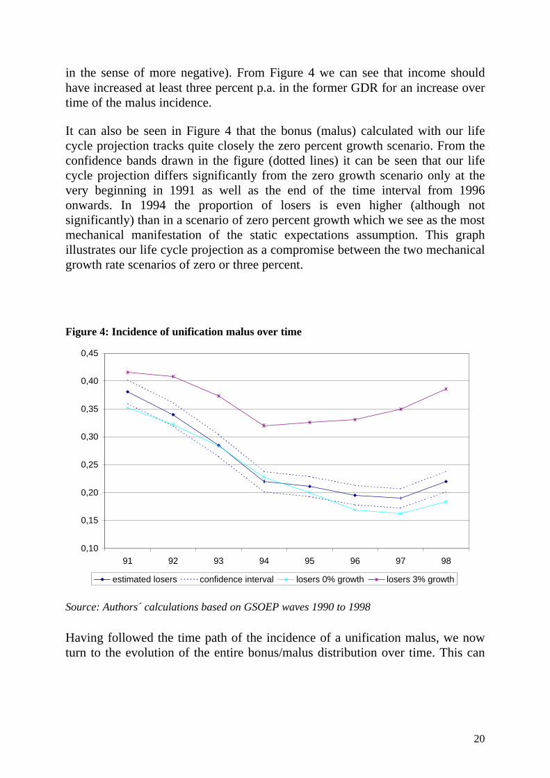
be seen in Figure 5 where kernel densities24 of the unification bonus (malus) areplotted for 1991 and 1998. The areas under the curves and to the left of theorigin are equal to the proportion of persons experiencing a unification malus forthe particular year. This proportion fell from 38 percent in 1991 to 22 percent in1998. But so did the variance of the bonuses. The existence of a substantialproportion of losers from unification can be seen as unifying the results from theincome inequality and income mobility literature discussed in the introduction.

Figure 5: Kernel density estimates of the German unification bonus 1991 and 1998


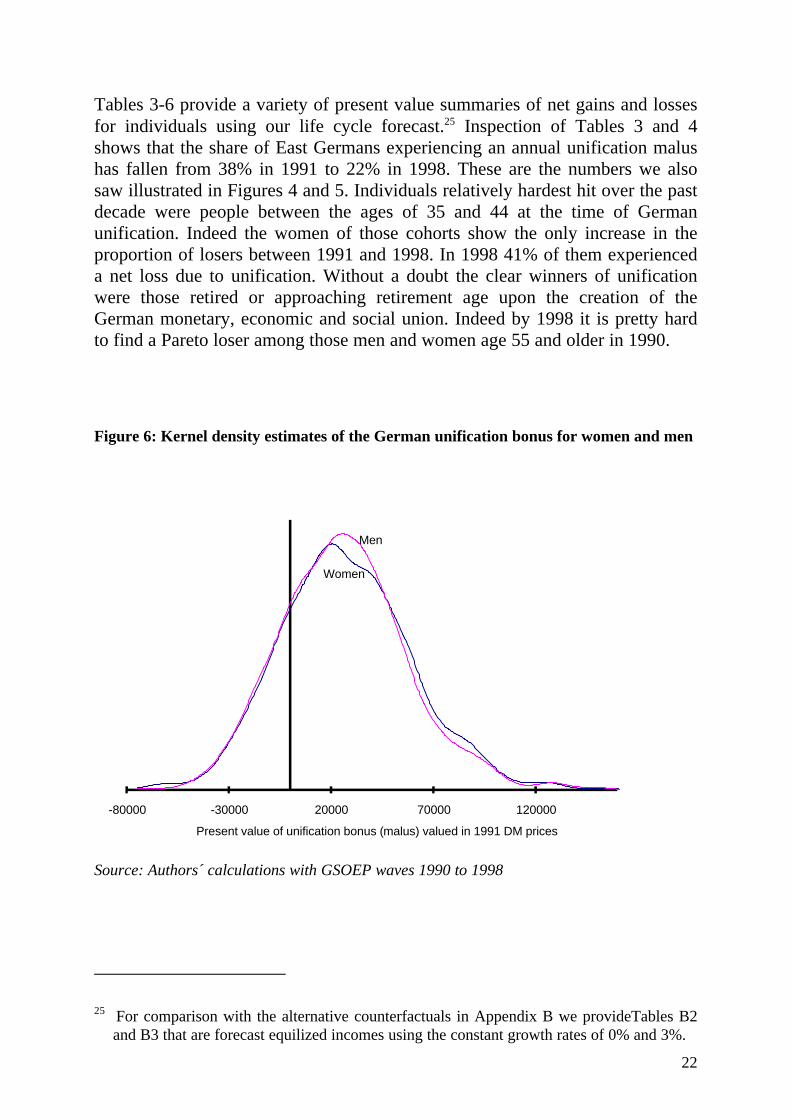
Comparing the kernel densities of the present value of the cumulative annualbonuses for 1990-98 for women and men separately in Figure 6, one does notsee a major difference between the sexes. The mode of the distribution forwomen is a little bit lower and occurs at a somewhat lower value of the presentvalue bonus.

24 For the kernel density estimation we used the Gaussian kernel. The density estimate isevaluated at 500 points and we used a bandwidth h that was chosen optimally according tothe formula 5/106.1 −⋅⋅= nshopt where s is the estimated standard deviation and n is thesample size.

1991

1998

-2000 -1000 0 1000 2000 3000

Monthly unification bonus (malus) valued in 1991 DM prices

22

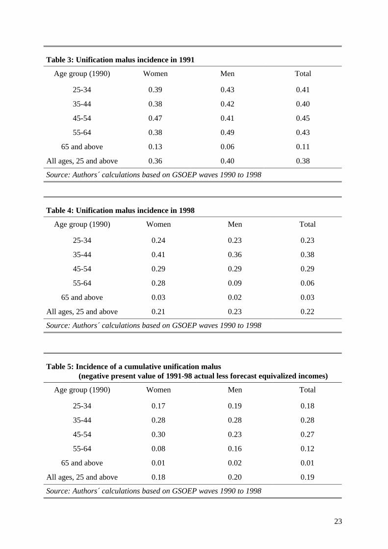
Tables 3-6 provide a variety of present value summaries of net gains and lossesfor individuals using our life cycle forecast.25 Inspection of Tables 3 and 4shows that the share of East Germans experiencing an annual unification malushas fallen from 38% in 1991 to 22% in 1998. These are the numbers we alsosaw illustrated in Figures 4 and 5. Individuals relatively hardest hit over the pastdecade were people between the ages of 35 and 44 at the time of Germanunification. Indeed the women of those cohorts show the only increase in theproportion of losers between 1991 and 1998. In 1998 41% of them experienceda net loss due to unification. Without a doubt the clear winners of unificationwere those retired or approaching retirement age upon the creation of theGerman monetary, economic and social union. Indeed by 1998 it is pretty hardto find a Pareto loser among those men and women age 55 and older in 1990.

Figure 6: Kernel density estimates of the German unification bonus for women and men

Source: Authors´ calculations with GSOEP waves 1990 to 1998

25 For comparison with the alternative counterfactuals in Appendix B we provideTables B2and B3 that are forecast equilized incomes using the constant growth rates of 0% and 3%.

Women

Men

-80000 -30000 20000 70000 120000

Present value of unification bonus (malus) valued in 1991 DM prices

23

Table 3: Unification malus incidence in 1991

Age group (1990) Women Men Total

25-34 0.39 0.43 0.41

35-44 0.38 0.42 0.40

45-54 0.47 0.41 0.45

55-64 0.38 0.49 0.43

65 and above 0.13 0.06 0.11

All ages, 25 and above 0.36 0.40 0.38


Table 4: Unification malus incidence in 1998


25-34 0.24 0.23 0.23

35-44 0.41 0.36 0.38

45-54 0.29 0.29 0.29

55-64 0.28 0.09 0.06

65 and above 0.03 0.02 0.03



Table 5: Incidence of a cumulative unification malus(negative present value of 1991-98 actual less forecast equivalized incomes)


25-34 0.17 0.19 0.18

35-44 0.28 0.28 0.28

45-54 0.30 0.23 0.27

55-64 0.08 0.16 0.12

65 and above 0.01 0.02 0.01



24

Table 5 may be regarded our preferred summary table according to which 19%of our sample suffered a cumulative present value unification malus through1998. We see the incidence of a unification malus is slightly greater for menthan for women, although among the middle-aged cohorts women have been hitharder with the highest cell incidence in Table 5 of 30% losers found for 45 to54 year-old women. One is also struck by extremely small proportion of losersamong the elderly.

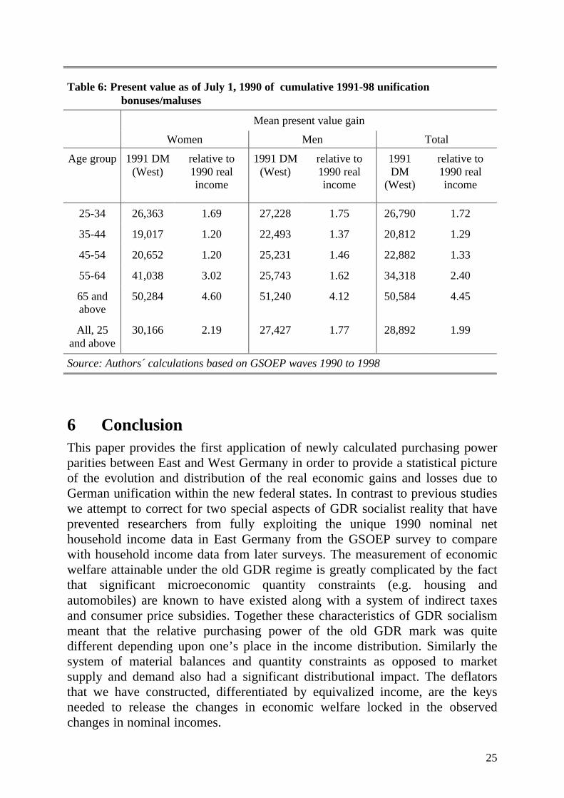
Granting the potential political importance of the incidence of a unificationmalus, one is curious to know the average size of the unification bonus which istabulated in Table 6 for the same age/sex groups. The present value ofcumulative unification bonuses is expressed both in 1991 DM West Germanprices as well as a percent of real adult equivalent income in the GDR in 1990.For all age-gender combinations we see that there was in fact a positive netunification bonus on average, i.e. winners could have compensated losers andremained winners in all cells of the table. We note that women between the agesof 35 and 44 at the time of German economic unification received the lowestaverage net cumulative bonus, especially when compared to their parents inretirement age with approximately 2.5 times larger average unification bonuses.Thus we see that gender differences in the unification bonus are swamped byage differences.

At this point it is most interesting to compare the results of direct public surveyswith the results of our calculations. The German weekly newspaper Die ZEIT26

on the occasion of the tenth anniversary of German unification in 2000 repeatedan opinion survey of East Germans it conducted in 1993. The new survey foundthat the proportion of self-reported losers from unification had fallen from 24 to19%. Another survey on subjective well-being in East Germany asked whetherindividual living conditions improved or deteriorated since 1990 (Habich, Noll,and Zapf 1999). Whereas in 1993 23% of the respondents claimed adeterioration, by 1998 this share had fallen to only 16%. For those who mightfind the combination of econometrics, assumption and data in this papersomewhat mysterious, perhaps the proportions of self-proclaimed unificationlosers from these public opinion surveys helps to demonstrate a broadconsistency between quite disparate and independent sources of evidence.

26 September 28, 2000.

25

Table 6: Present value as of July 1, 1990 of cumulative 1991-98 unificationbonuses/maluses

Mean present value gain

Women Men Total

Age group 1991 DM(West)

relative to1990 realincome

1991 DM(West)


1991DM

(West)


25-34 26,363 1.69 27,228 1.75 26,790 1.72

35-44 19,017 1.20 22,493 1.37 20,812 1.29

45-54 20,652 1.20 25,231 1.46 22,882 1.33

55-64 41,038 3.02 25,743 1.62 34,318 2.40

65 andabove

50,284 4.60 51,240 4.12 50,584 4.45

All, 25and above

30,166 2.19 27,427 1.77 28,892 1.99


6 ConclusionThis paper provides the first application of newly calculated purchasing powerparities between East and West Germany in order to provide a statistical pictureof the evolution and distribution of the real economic gains and losses due toGerman unification within the new federal states. In contrast to previous studieswe attempt to correct for two special aspects of GDR socialist reality that haveprevented researchers from fully exploiting the unique 1990 nominal nethousehold income data in East Germany from the GSOEP survey to comparewith household income data from later surveys. The measurement of economicwelfare attainable under the old GDR regime is greatly complicated by the factthat significant microeconomic quantity constraints (e.g. housing andautomobiles) are known to have existed along with a system of indirect taxesand consumer price subsidies. Together these characteristics of GDR socialismmeant that the relative purchasing power of the old GDR mark was quitedifferent depending upon one’s place in the income distribution. Similarly thesystem of material balances and quantity constraints as opposed to marketsupply and demand also had a significant distributional impact. The deflatorsthat we have constructed, differentiated by equivalized income, are the keysneeded to release the changes in economic welfare locked in the observedchanges in nominal incomes.

26

Consistent with the general macroeconomic picture, we find a clear andoverwhelming economic bonus on average for East Germans. Just as much apart of the story of postwall economic reconstruction are those who havesuffered a unification malus, understood here to be a negative present-value ofannual differences between the course of actual income and a counterfactualforecast of income in a frozen GDR. About 19 percent of the East Germanpopulation older than 25 in 1990 and who remained in the sample until 1998 areidentified as having experienced a unification malus. We have found that incontrast to what has been observed in other economies in transition from the oldsocialist order, elderly East Germans have not only gained much more thanother age groups, but that for all intents and purpose our sample of East Germanelderly survived the fall of communism in a way that both Helmut Kohl andVilfredo Pareto could score as an improvement in economic welfare. At theother end of the bonus distribution, the smallest average unification bonus wasfound for women between the ages of 35 and 44 at the time of Germanunification. Thirty percent of that group were identified as unification losers.

We are confident that our estimated proportion of economic ‘losers’ representsan upper bound since it was calculated under the assumption of staticexpectations for our GDR counterfactual. The GDR economy was riding adownward trend at the time of its political demise and few believe that it wouldhave been able to even maintain 1989 living standards over the past decade.Thus while allowing for the psychological salience of the last days of the GDR,as an economic matter we have almost certainly overstated the number ofeconomic losers.

To break the stranglehold of quantity constraints on the interpretation ofconsumer behavior under socialism it was necessary to import demandparameters from elsewhere. For most economists it would appear natural toassume that East Germans were actually just West Germans who weresignificantly poorer and more repressed. This critical assumption is necessary tojustify using West German household budgets to construct deflators for EastGerman households. Indeed had socialism changed consumer preferences, theuse of West German preferences to interpret East German reality wouldrepresent a fundamental misspecification. Few would confuse the GDR withNorth Korea however.

Our attention has been limited to household income and its power to purchaseconsumer goods and services. The transformation of the East German economyof course involved a fundamental redefinition of many property rights. Thecapital gains from owning a modest family house on prime postwall land, thevalue of the family farm or the loss of a bargain housing rental to the heirs of anexpropriated owner are not touched upon in this paper. In particular we have notattempted to assess the unification bonus with respect to asset holdings – as

27

opposed to equivalent income in this study – due to the lack of such data in theGSOEP.

It is also important to add what may seem to be an obvious qualification giventhe title of the paper, we have nothing to say here about the unification bonus ormalus for West Germans. Between four and five percent of West German GDPevery year has been the size of the net West to East transfer during the pastdecade. Comparing the average East German welfare gains with the averageWest German losses is a most interesting question, though probably a better useof scarce research time would be to identify the policy mistakes that still leavenearly one third of the East German potential working force in a social safety netfinanced by West Germany.

Having struggled to extract meaning from these data, we feel an obligation toprovide a short list of promising leads for future research. The first item is anempirical matter regarding the housing rental component of the deflators usedhere. The critical housing cost PPP to bridge the gap between East and West in1993 was not part of the survey of the German Federal Statistical Office ofprices and is better characterized as expert opinion than a statistical averagefrom a well designed survey. Furthermore housing constitutes probably thesingle most important expenditure item in family budgets and happens to haveone of the most dramatic relative price changes in the move from socialism tosocial market.

The issue of the appropriate equivalence scale within a market economy at apoint in time is just about as subtle as any in the measurement of economicwelfare (cf. Lewbel 1997). Our choice of using the modified OECD scale hasonly the virtue in being comparable with a vast empirical literature on incomedistribution and while we find ourselves good company, we still believe that it isunlikely that one scale is going to fit all places and all times, least of all foreconomic transitions from central planning to market allocation. It is certainlyour hope that future researchers will be able to remedy this weakness.

While the deflators upon which our estimates of the unification bonus are baseddo attempt to correct for the spillover of demand across aggregate spendingcategories, say, from consumer electronics to alcoholic beverages, this is onlypart of the story. What is still missing is the breadth of product variety in amarket economy that was missing in the centrally planned economies. Forexample one could travel, but as a general rule one could not travel on holiday inthe West. What is the value of the introduction of that single ‘new product’ withthe fall of the Wall? This has been found to be an important shortcoming oftraditional consumer price indexes for market economies, e.g. Hausman’s (1999)study that documents the welfare gains from the introduction of the new product

28

cell-phones in the U.S. To that extent we have further reason to believe that ourestimates of unification ‘losers’ is an upper bound.

We conclude on a substantive note and point to a disturbing pattern that one cansee in the evolution of the annual unification bonus over time. Completelyconsistent with the marked slowdown in GDP as seen in the first set of figuresof this paper, the number of ‘losers’ appears to be rising at the end of our periodof investigation. This comes as no surprise to those familiar with the economicand political situation in the new federal states. One may presume that GDRpolicy makers did not intend to waste a over a quarter of the East German laborforce either. What the communist leadership lacked was the capacity to tap theWest German taxpayer on anything approaching the scale of the unificationbonus that we have estimated.

29

References

Akerlof, G., Rose, A., Yellen, J. and Hessenius, H. (1991). East Germany infrom the cold: the economic aftermath of currency union. BrookingsPapers for Economic Activity, Vol. I, 1-101.

Atkinson, A.B.; Rainwater, L. and T.M. Smeeding (1995): Income Distributionin OECD Countries: Evidence from the Luxembourg Income Study (LIS),Social Policy Studies #18, OECD, Paris.

Burkhauser, R.V.; Smeeding, T.M. and J. Merz (1996): „Relative Inequality andPoverty in Germany and the United States Using AlternativeEquivalence Scales, Review of Income and Wealth, 42,4, 381-400..

Collier, I. L. (1986): Effective Purchasing Power in a Quantity ConstrainedEconomy: An Estimate for the German Democratic Republic, Review ofEconomics and Statistics, 58, 1, 24-32.

Collier, I.L. (1989): The Measurement and Interpretation of Real Consumptionand Purchasing Power Parity for a Quantity Constrained Economy: TheCase of East and West Germany, Economica, 56, 109-120.

Collier, I.L. (2001): The DM and the Ossi Consumer, Freie Universität Berlin,Working Paper.

Deutsches Institut für Wirtschaftsforschung Berlin, Institut für Weltwirtschaft ander Universität Kiel, Institut für Wirtschaftsforschung Halle (1999):Gesamtwirtschaftliche und unternehmerische Anpassungsfortschritte inOstdeutschland, DIW Wochenbericht. 1/1999, pp-pp.

Franz, W. and V. Steiner (1999): Wages in the East German Transition Process– Facts and Explanations, ZEW Discussion paper 99-40, Mannheim.

Gottschalk, P. and T. M. Smeeding (1997): Cross-National Comparisons ofEarnings and Income Inequality, Journal of Economic Literature, 35,633-687.

Gottschalk, P. and T. M. Smeeding (1998): Empirical Evidence on IncomeInequality in Industrialized Countries, Luxembourg Income StudyWorking Paper Series No. 154.

Grabka, M. and B. Otto (2001): Angleichung der Markteinkommen privaterHaushalte in Ost- und Westdeutschland nicht in Sicht, DIW-Wochenbericht 4/2001, 51-56.

Habich, R., Noll, H.-H. and W. Zapf (1999): Subjektives Wohlbefinden inOstdeutschland nähert sich westdeutschem Niveau. Ergebnisse desWohlfahrtssurveys 1998, in: ISI-Informationsdientst Soziale Indikatoren,Ausgabe 22: 1-6.

30

Hauser, R. (1992): Die personelle Einkommensverteilung in den alten und neuenBundesländern vor der Vereinigung – Probleme eines empirischenVergleichs und der Abschätzung von Entwicklungstendenzen. In:Kleinhenz, G. (Ed.): Sozialpolitik im vereinten Deutschland II. Schriftendes Vereins für Sozialpolitik. Duncker & Humblot. Berlin.

Hauser, R. and H. Fabig (1999): Labor Earnings and Household IncomeMobility in Reunified Germany: A Comparison of the Eastern andWestern States, Review of Income and Wealth 45(3): 303-324.

Hauser, R. and G. Wagner (1996): Die Einkommensverteilung inOstdeutschland – Darstellung, Vergleich und Determinanten für dieJahre 1990 bis 1994. In: Hauser, R. (Ed.): Sozialpolitik im vereintenDeutschland III. Schriften des Vereins für Sozialpolitik. Duncker &Humblot. Berlin.

Hausman, J. (1999): Cellular Phones, New products, and the CPI, Journal ofBusiness and Economics Statistics, 17, 2, 188-194.

Krause, P. and R. Habich (1993): Einkommensverteilung und Einkommens-zufriedenheit in ostdeutschen Privathaushalten, DIW-Wochenbericht6/93, 55-59.

Lewbel, A. (1997). Consumer Demand Systems and Household EquivalenceScales. In Pesaran, M.H. and P. Schmidt (Eds.): Handbook of AppliedEconometrics. Volume II: Microeconomics. Blackwell Publishers.

Ministerrat der Deutschen Demokratischen Republik, StaatlicheZentralverwaltung für Statistik, Zentrales Zählbüro (1989):Haushaltseinkommen und Ausstattung der Haushalte von Arbeitern undAngestellten 1980-1988.

Neary, J.P. and Roberts, K.W.S. (1980): The theory of household behaviourunder rationing. European Economic Review 13, 25.42.

Projektgruppe Sozio-oekonomisches Panel (1995): Das Sozio-oekonomischePanel (SOEP) im Jahre 1994, Vierteljahreshefte zurWirtschaftsforschung 64(1): 5-13.

Puhani, P. and V. Steiner (1996): Die Entwicklung der Lohnstruktur imostdeutschen Transformationsprozeß, ZEW Discussion paper 96-03,Mannheim.

Rothbarth, Erwin (1941): The measurement of changes in real income underconditions of rationing. Review of Economic Studies 8, 100-107.

Schürer, G. (1992): Analyse der ökonomischen Lage der DDR mitSchlußfolgerungen. Deutschland Archiv 25 (October 1992), 1112-1120.

Statistisches Bundesamt (1984-1998): Einnahmen und Ausgaben ausgewählterprivater Haushalte. Fachserie 15. Reihe 1.

31

Statistisches Bundesamt (1984-1998): Preise und Preisindizes für dieLebenshaltung. Fachserie 17. Reihe 7, Preise und Preisindizes für dieLebenshaltung 1993.

Statistisches Bundesamt (1992a): Preise. Heft 32 Preisindex für dieLebenshaltung Mai 1990 bis April 1991 für das Gebiet der LänderMecklenburg-Vorpommern, Brandenburg, Sachsen-Anhalt, Sachsen,Thüringen sowie Berlin (Ost).

Statistisches Bundesamt (1992b). Preise. Heft 59. Preisindex für dieLebenshaltung für das Gebiet der Länder Mecklenburg-Vorpommern,Brandenburg, Sachsen-Anhalt, Sachsen, Thüringen sowie Berlin (Ost).Juli 1990 bis Dezember 1991.

Statistisches Bundesamt (1993a). Sonderreihe mit Beiträgen für das Gebiet derehemaligen DDR. Heft 5. Einnahmen und Ausgaben privater Haushalte1985 bis 1990.

Steiner, V. and F. Kraus (1996): Aufsteiger und Absteiger in der ostdeutschenEinkommensverteilung: 1989-1993, in: Diewald, M. and K. U. Mayer(Eds.): Zwischenbilanz der Wiedervereinigung – Strukturwandel undMobilität im Transformationsprozeß, Opladen, 189-212.

Ströhl, Gerd (1994). Zwischenörtlicher Vergleich des Verbraucherpreisniveausin 50 Städten. Wirtschaft und Statistik 6/1994: 415-434.

Texte zur Deutschlandpolitik. Reihe III/Band 8a-1990.

Wagner, G. and R.V. Burkhauser and F. Behringer (1993): The EnglishLanguage Public Use File of the German Socio-Economic Panel Study,The Journal of Human Resources 28(2): 429-433.

32

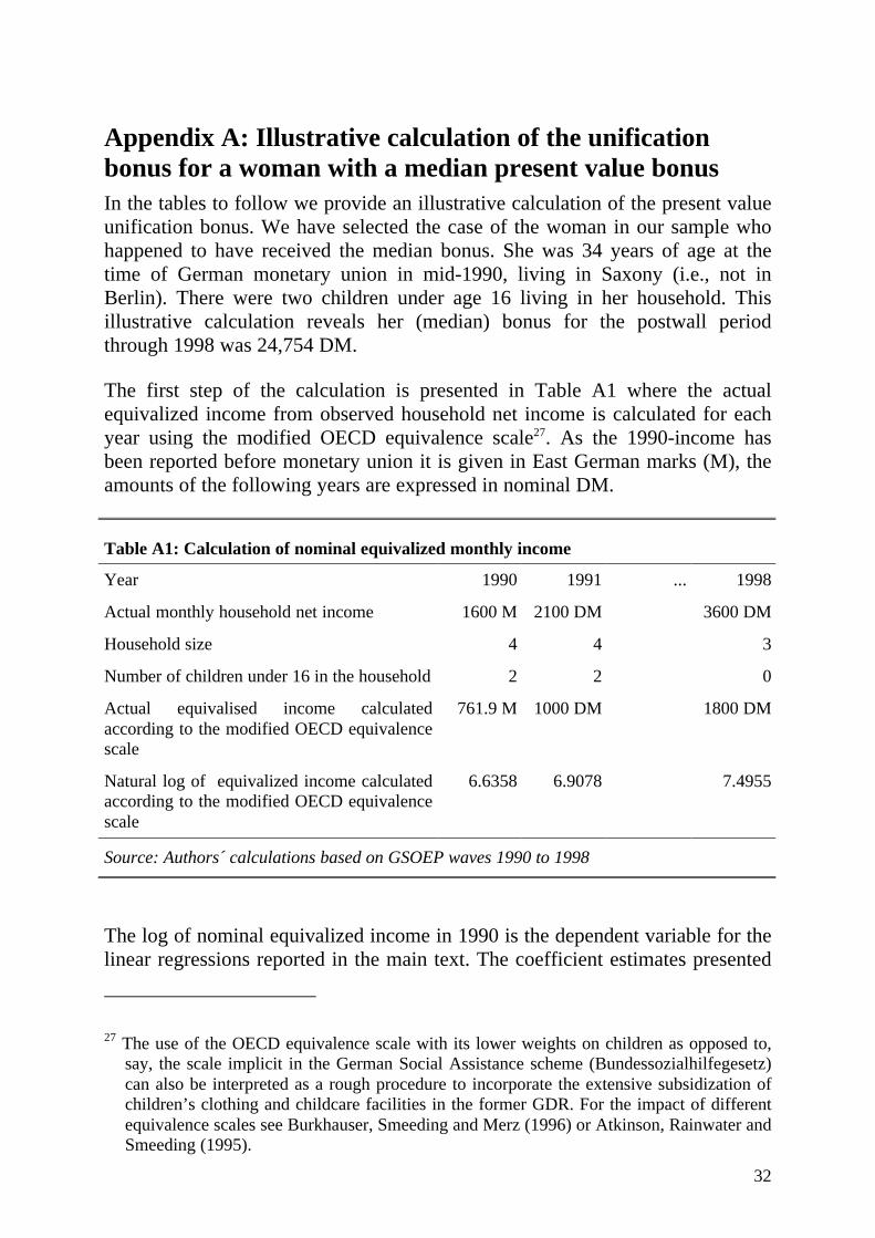
Appendix A: Illustrative calculation of the unificationbonus for a woman with a median present value bonusIn the tables to follow we provide an illustrative calculation of the present valueunification bonus. We have selected the case of the woman in our sample whohappened to have received the median bonus. She was 34 years of age at thetime of German monetary union in mid-1990, living in Saxony (i.e., not inBerlin). There were two children under age 16 living in her household. Thisillustrative calculation reveals her (median) bonus for the postwall periodthrough 1998 was 24,754 DM.

The first step of the calculation is presented in Table A1 where the actualequivalized income from observed household net income is calculated for eachyear using the modified OECD equivalence scale27. As the 1990-income hasbeen reported before monetary union it is given in East German marks (M), theamounts of the following years are expressed in nominal DM.

Table A1: Calculation of nominal equivalized monthly income

Year 1990 1991 ... 1998

Actual monthly household net income 1600 M 2100 DM 3600 DM

Household size 4 4 3

Number of children under 16 in the household 2 2 0

Actual equivalised income calculatedaccording to the modified OECD equivalencescale

761.9 M 1000 DM 1800 DM

Natural log of equivalized income calculatedaccording to the modified OECD equivalencescale

6.6358 6.9078 7.4955


The log of nominal equivalized income in 1990 is the dependent variable for thelinear regressions reported in the main text. The coefficient estimates presented

27 The use of the OECD equivalence scale with its lower weights on children as opposed to,say, the scale implicit in the German Social Assistance scheme (Bundessozialhilfegesetz)can also be interpreted as a rough procedure to incorporate the extensive subsidization ofchildren’s clothing and childcare facilities in the former GDR. For the impact of differentequivalence scales see Burkhauser, Smeeding and Merz (1996) or Atkinson, Rainwater andSmeeding (1995).

33

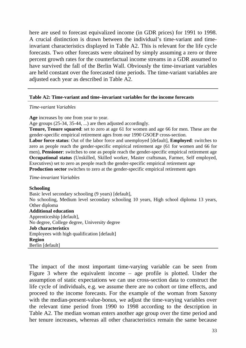
here are used to forecast equivalized income (in GDR prices) for 1991 to 1998.A crucial distinction is drawn between the individual’s time-variant and time-invariant characteristics displayed in Table A2. This is relevant for the life cycleforecasts. Two other forecasts were obtained by simply assuming a zero or threepercent growth rates for the counterfactual income streams in a GDR assumed tohave survived the fall of the Berlin Wall. Obviously the time-invariant variablesare held constant over the forecasted time periods. The time-variant variables areadjusted each year as described in Table A2.

Table A2: Time-variant and time–invariant variables for the income forecasts

Time-variant Variables

Age increases by one from year to year.Age groups (25-34, 35-44, ...) are then adjusted accordingly.Tenure, Tenure squared: set to zero at age 61 for women and age 66 for men. These are thegender-specific empirical retirement ages from our 1990 GSOEP cross-section.Labor force status: Out of the labor force and unemployed [default], Employed: switches tozero as people reach the gender-specific empirical retirement age (61 for women and 66 formen), Pensioner: switches to one as people reach the gender-specific empirical retirement ageOccupational status (Unskilled, Skilled worker, Master craftsman, Farmer, Self employed,Executives) set to zero as people reach the gender-specific empirical retirement ageProduction sector switches to zero at the gender-specific empirical retirement ages

Time-invariant Variables

SchoolingBasic level secondary schooling (9 years) [default],No schooling, Medium level secondary schooling 10 years, High school diploma 13 years,Other diplomaAdditional educationApprenticeship [default],No degree, College degree, University degreeJob characteristicsEmployees with high qualification [default]RegionBerlin [default]

The impact of the most important time-varying variable can be seen fromFigure 3 where the equivalent income – age profile is plotted. Under theassumption of static expectations we can use cross-section data to construct thelife cycle of individuals, e.g. we assume there are no cohort or time effects, andproceed to the income forecasts. For the example of the woman from Saxonywith the median-present-value-bonus, we adjust the time-varying variables overthe relevant time period from 1990 to 1998 according to the description inTable A2. The median woman enters another age group over the time period andher tenure increases, whereas all other characteristics remain the same because

34

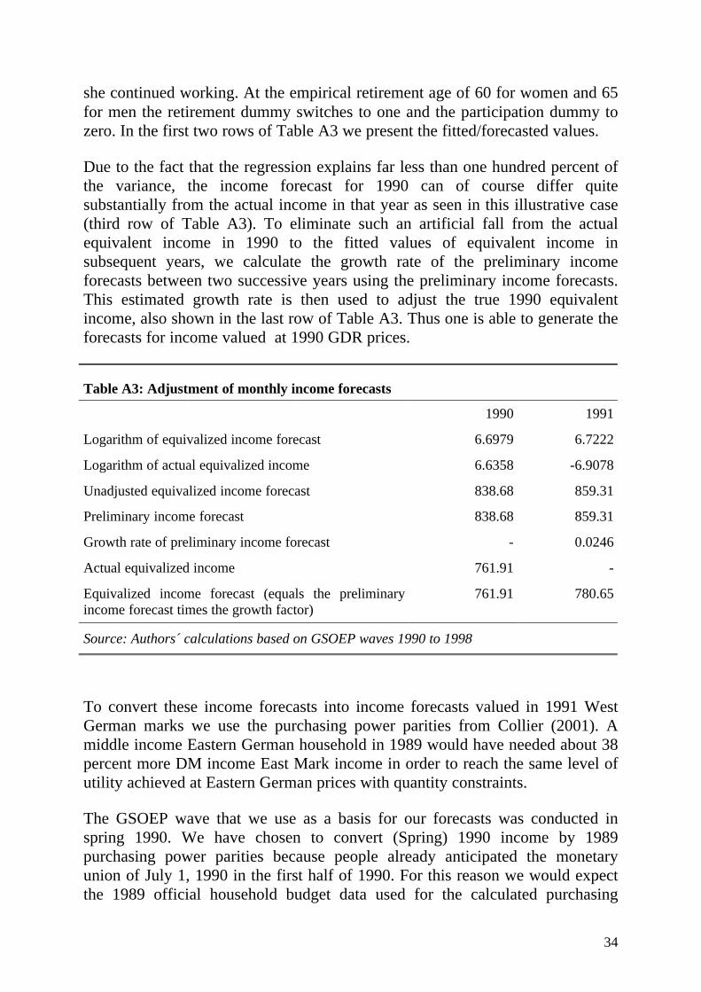
she continued working. At the empirical retirement age of 60 for women and 65for men the retirement dummy switches to one and the participation dummy tozero. In the first two rows of Table A3 we present the fitted/forecasted values.

Due to the fact that the regression explains far less than one hundred percent ofthe variance, the income forecast for 1990 can of course differ quitesubstantially from the actual income in that year as seen in this illustrative case(third row of Table A3). To eliminate such an artificial fall from the actualequivalent income in 1990 to the fitted values of equivalent income insubsequent years, we calculate the growth rate of the preliminary incomeforecasts between two successive years using the preliminary income forecasts.This estimated growth rate is then used to adjust the true 1990 equivalentincome, also shown in the last row of Table A3. Thus one is able to generate theforecasts for income valued at 1990 GDR prices.

Table A3: Adjustment of monthly income forecasts

1990 1991

Logarithm of equivalized income forecast 6.6979 6.7222

Logarithm of actual equivalized income 6.6358 -6.9078

Unadjusted equivalized income forecast 838.68 859.31

Preliminary income forecast 838.68 859.31

Growth rate of preliminary income forecast - 0.0246

Actual equivalized income 761.91 -

Equivalized income forecast (equals the preliminaryincome forecast times the growth factor)

761.91 780.65


To convert these income forecasts into income forecasts valued in 1991 WestGerman marks we use the purchasing power parities from Collier (2001). Amiddle income Eastern German household in 1989 would have needed about 38percent more DM income East Mark income in order to reach the same level ofutility achieved at Eastern German prices with quantity constraints.

The GSOEP wave that we use as a basis for our forecasts was conducted inspring 1990. We have chosen to convert (Spring) 1990 income by 1989purchasing power parities because people already anticipated the monetaryunion of July 1, 1990 in the first half of 1990. For this reason we would expectthe 1989 official household budget data used for the calculated purchasing

35

power parities to be cleaner in the sense of being more representative of whatthe GDR economy really looked like before monetary union.

As Gottschalk and Smeeding (1998) have noted in the context of absoluteinternational income comparisons, it is questionable “whether a single index isappropriate for all points in the distribution”. Precisely for this reason we use thethree different purchasing power parities corresponding to different points of theGDR household income distribution as estimated by Collier (2001).

We have transformed reported household incomes by using the modified OECDequivalence scale under the assumption that in the type II and III households oneof the two children is under age sixteen and the other is older. Thus we“equivilize” the household incomes in the three household types by dividing by1.5 for type I and 2.3 for both types II and III.

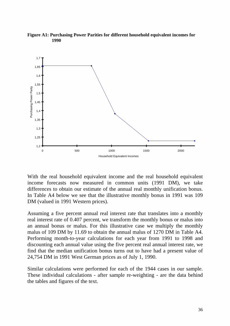
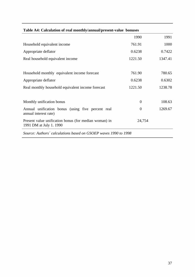
These three household equivalent incomes with their respective purchasingpower parities have been plotted using linear interpolation between the points asseen in Figure A1. With this empirical relationship between equivilized incomeand purchasing power parity of that income, we are able to convert nominal1990 East German household equivalent incomes into 1991 DM values. Thisconversion is shown for our illustrative case of the median present-value-bonuswoman in Table A4. Because the household equivalent income for this case is762 Eastern Marks in 1990, slightly exceeding the first threshold of 707 Marksin Figure A1, her equivilized income has been deflated by a factor of 0.6238obtained by interpolation. This results in a monthly real household equivalentincome of 1222 in 1990 valued in DM for the year 1991.

For 1991 the median bonus woman had a forecast household equivalent income(recall that counterfactual incomes are always valued in constant GDR Marks)of 781 DM. This amount is slightly higher than her income in 1990 and so ahigher deflator of 0.6302 is used to yield a real household equivalent incomeforecast of 1239 DM (1991) as seen in Table A4.

Similarly deflators for all other years are used to deflate observed monthlynominal incomes from GSOEP –the disposable income for eastern Germanhouseholds in unified Germany- to obtain real monthly incomes valued in 1991DM.

36

Figure A1: Purchasing Power Parities for different household equivalent incomes for1990

With the real household equivalent income and the real household equivalentincome forecasts now measured in common units (1991 DM), we takedifferences to obtain our estimate of the annual real monthly unification bonus.In Table A4 below we see that the illustrative monthly bonus in 1991 was 109DM (valued in 1991 Western prices).

Assuming a five percent annual real interest rate that translates into a monthlyreal interest rate of 0.407 percent, we transform the monthly bonus or malus intoan annual bonus or malus. For this illustrative case we multiply the monthlymalus of 109 DM by 11.69 to obtain the annual malus of 1270 DM in Table A4.Performing month-to-year calculations for each year from 1991 to 1998 anddiscounting each annual value using the five percent real annual interest rate, wefind that the median unification bonus turns out to have had a present value of24,754 DM in 1991 West German prices as of July 1, 1990.

Similar calculations were performed for each of the 1944 cases in our sample.These individual calculations - after sample re-weighting - are the data behindthe tables and figures of the text.

1,2

1,25

1,3

1,35

1,4

1,45

1,5

1,55

1,6

1,65

1,7

0 500 1000 1500 2000

Household Equivalent Incomes

Pur

chas

ing

Pow

er P

arity

37

Table A4: Calculation of real monthly/annual/present-value bonuses

1990 1991

Household equivalent income 761.91 1000

Appropriate deflator 0.6238 0.7422

Real household equivalent income 1221.50 1347.41

Household monthly equivalent income forecast 761.90 780.65

Appropriate deflator 0.6238 0.6302

Real monthly household equivalent income forecast 1221.50 1238.78

Monthly unification bonus 0 108.63

Annual unification bonus (using five percent realannual interest rate)

0 1269.67

Present value unification bonus (for median woman) in1991 DM at July 1. 1990

24,754


38

Appendix B

Table B1: Sample characteristics 1990

Women MenMean Stan. Dev. Mean Stan. Dev.

Individual characteristicsAge 45.27 13.39 44.15 11.86Married .78 .41 .88 .32

Schooling(Difference from basic levelsecondary schooling, 9 years)

No schooling .003 .05 .004 .06Medium level secondary

schooling, 10 years.45 .50 .44 .50

High school diploma, 13 years .12 .32 .19 .39Other .01 .10 .007 .08

Additional education (Differencefrom apprenticeship)

No degree .12 .32 .03 .16College degree .24 .43 .27 .44University degree .08 .27 .14 .35

Job characteristicsUnskilled white/blue collar .18 .38 .07 .25Skilled worker .11 .32 .34 .47Master craftsman .01 .11 .07 .25Farmer .05 .21 .12 .32Self employed .02 .13 .03 .18Employees with high

qualification.38 .49 .25 .44

Executives .01 .11 .03 .17Tenure 10.23 10.34 14.05 11.60Employed .76 .42 .91 .28Pensioner .15 .36 .06 .23

Region(Difference from East Berlin)

Mecklenburg-Vorpommern .11 .31 .11 .31Brandenburg .15 .35 .15 .36Sachsen-Anhalt .19 .39 .18 .39Thüringen .19 .39 .19 .39Sachsen .30 .46 .30 .46

Household characteristicsChildren under 16 years in

household.48 .50 .50 .50

Household size 3.04 1.18 3.19 1.08Total household income 1832.38 720.39 1963.37 634.41Equivalized income (modified

OECD-scale)979.15 303.49 1029.35 291.90

Number of observations 1142 968


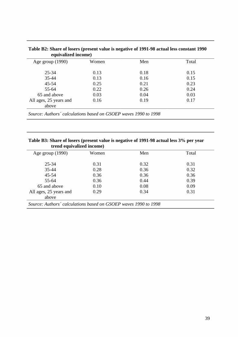
39

Table B2: Share of losers (present value is negative of 1991-98 actual less constant 1990equivalized income)


25-34 0.13 0.18 0.1535-44 0.13 0.16 0.1545-54 0.25 0.21 0.2355-64 0.22 0.26 0.24

65 and above 0.03 0.04 0.03All ages, 25 years and

above0.16 0.19 0.17


Table B3: Share of losers (present value is negative of 1991-98 actual less 3% per yeartrend equivalized income)


25-34 0.31 0.32 0.3135-44 0.28 0.36 0.3245-54 0.36 0.36 0.3655-64 0.36 0.44 0.39

65 and above 0.10 0.08 0.09All ages, 25 years and

above0.29 0.34 0.31


Documents

The unification bonus (malus) in postwall Eastern Germany