The Unsteady Aerodynamics Module for FAST 8aerodynamics routines. AeroDyn is an aerodynamics module comprised of four submodels: rotor wake/induction, blade airfoil aerodynamics, tower

NREL is a national laboratory of the U.S. Department of Energy Office of Energy Efficiency & Renewable Energy Operated by the Alliance for Sustainable Energy, LLC This report is available at no cost from the National Renewable Energy Laboratory (NREL) at www.nrel.gov/publications.

Contract No. DE-AC36-08GO28308

Technical Report NREL/TP-5000-66347 November 2019

The Unsteady Aerodynamics Module for FAST 8

Rick Damiani and Greg Hayman

National Renewable Energy Laboratory

NREL is a national laboratory of the U.S. Department of Energy Office of Energy Efficiency & Renewable Energy Operated by the Alliance for Sustainable Energy, LLC This report is available at no cost from the National Renewable Energy Laboratory (NREL) at www.nrel.gov/publications.

Contract No. DE-AC36-08GO28308

National Renewable Energy Laboratory 15013 Denver West Parkway Golden, CO 80401 303-275-3000 • www.nrel.gov

Technical Report NREL/TP-5000-66347 November 2019

The Unsteady Aerodynamics Module for FAST 8

Rick Damiani and Greg Hayman

National Renewable Energy Laboratory

Suggested Citation Damiani, Rick, and Greg Hayman. 2019. The Unsteady Aerodynamics Module for FAST 8. Golden, CO: National Renewable Energy Laboratory. NREL/TP-5000-66347. https://www.nrel.gov/docs/fy20osti/66347.pdf.

https://www.nrel.gov/docs/fy20osti/66347.pdf

NOTICE

This work was authored by the National Renewable Energy Laboratory, operated by Alliance for Sustainable Energy, LLC, for the U.S. Department of Energy (DOE) under Contract No. DE-AC36-08GO28308. Funding provided by the U.S. Department of Energy Office of Energy Efficiency and Renewable Energy Wind Energy Technologies Office. The views expressed herein do not necessarily represent the views of the DOE or the U.S. Government.

This report is available at no cost from the National Renewable Energy Laboratory (NREL) at www.nrel.gov/publications.

U.S. Department of Energy (DOE) reports produced after 1991 and a growing number of pre-1991 documents are available free via www.OSTI.gov.

Cover Photos by Dennis Schroeder: (clockwise, left to right) NREL 51934, NREL 45897, NREL 42160, NREL 45891, NREL 48097, NREL 46526.

NREL prints on paper that contains recycled content.

http://www.nrel.gov/publications

http://www.osti.gov/

Executive Summary

The new modularization framework of FAST v.8 (Jonkman 2013) was accompanied by a complete overhaul of the

aerodynamics routines. AeroDyn is an aerodynamics module comprised of four submodels: rotor wake/induction,

blade airfoil aerodynamics, tower influence on the blade nodes, and tower drag. Throughout the software overhaul,

several improvements to the original theoretical treatments were achieved, including more accurate skewed-wake and

unsteady airfoil aerodynamics, and the possibility of modeling highly flexible and curved blades.

Under asymmetric conditions, such as wind shear, yawed, and tilted flow, the individual blade elements undergo vari-

ations in angle of attack that lead to unsteady aerodynamics phenomena, which can no longer be captured through

the static airfoil lift and drag look-up tables. This document covers the main theory and the organization of the mod-

ularization framework of the new unsteady aerodynamics submodule (UAM)1, which includes unsteady aerodynam-

ics under attached flow conditions and dynamic stall. The UAM can be called by either blade element momentum

theory (only interface discussed in this report), or other future wake models (e.g.,dynamic blade element momentum

theory, or generalized dynamic wake).

1UAM is a submodule to OpenFAST’s aerodynamics module (AeroDyn), but we will continue using the term module for simplicity.

iii

This report is available at no cost from the National Renewable Energy Laboratory at www.nrel.gov/publications

Acknowledgments

This document was reviewed and improved thanks to the input provided by Michael Sprague, Jason Jonkman, and

Bonnie Jonkman.

iv


Table of Contents

List of Acronyms . . . . . . . . . . . . . . . . . . . . . . . . . . . . . . . . . . . . . . . . . . . . . . . . 2

List of Symbols . . . . . . . . . . . . . . . . . . . . . . . . . . . . . . . . . . . . . . . . . . . . . . . . . 2

List of Subscripts and Superscripts . . . . . . . . . . . . . . . . . . . . . . . . . . . . . . . . . . . . . . . 8

List of Greek Symbols . . . . . . . . . . . . . . . . . . . . . . . . . . . . . . . . . . . . . . . . . . . . . 8

1 Overview . . . . . . . . . . . . . . . . . . . . . . . . . . . . . . . . . . . . . . . . . . . . . . . . . . . . 11

1.1 Unsteady Attached Flow and Its Indicial Treatment . . . . . . . . . . . . . . . . . . . . . . . . . . . 12

1.1.1 Normal Force . . . . . . . . . . . . . . . . . . . . . . . . . . . . . . . . . . . . . . . . . . . 14

1.1.2 Chordwise Force . . . . . . . . . . . . . . . . . . . . . . . . . . . . . . . . . . . . . . . . . 17

1.1.3 Pitching Moment . . . . . . . . . . . . . . . . . . . . . . . . . . . . . . . . . . . . . . . . . 18

1.2 TE Flow Separation . . . . . . . . . . . . . . . . . . . . . . . . . . . . . . . . . . . . . . . . . . . . 19

1.2.1 Normal Force . . . . . . . . . . . . . . . . . . . . . . . . . . . . . . . . . . . . . . . . . . . 20

1.2.2 Chordwise Force . . . . . . . . . . . . . . . . . . . . . . . . . . . . . . . . . . . . . . . . . 21

1.2.3 Pitching Moment . . . . . . . . . . . . . . . . . . . . . . . . . . . . . . . . . . . . . . . . . 21

1.3 Dynamic Stall . . . . . . . . . . . . . . . . . . . . . . . . . . . . . . . . . . . . . . . . . . . . . . . 22

1.3.1 Normal Force . . . . . . . . . . . . . . . . . . . . . . . . . . . . . . . . . . . . . . . . . . . 22

1.3.2 Chordwise Force . . . . . . . . . . . . . . . . . . . . . . . . . . . . . . . . . . . . . . . . . 23

1.3.3 Pitching Moment . . . . . . . . . . . . . . . . . . . . . . . . . . . . . . . . . . . . . . . . . 23

2 Inputs, Outputs, Parameters, States, and Implementation of UA . . . . . . . . . . . . . . . . . . . . . 24

2.1 Init_Inputs . . . . . . . . . . . . . . . . . . . . . . . . . . . . . . . . . . . . . . . . . . . . . . . . . 24

2.2 Inputs u . . . . . . . . . . . . . . . . . . . . . . . . . . . . . . . . . . . . . . . . . . . . . . . . . . 25

2.3 Outputs y . . . . . . . . . . . . . . . . . . . . . . . . . . . . . . . . . . . . . . . . . . . . . . . . . 25

2.4 States xd

. . . . . . . . . . . . . . . . . . . . . . . . . . . . . . . . . . . . . . . . . . . . . . . . . . 25

2.5 Parameters p . . . . . . . . . . . . . . . . . . . . . . . . . . . . . . . . . . . . . . . . . . . . . . . . 26

2.6 UA Implementation . . . . . . . . . . . . . . . . . . . . . . . . . . . . . . . . . . . . . . . . . . . . 27

2.6.1 UA_Init Routine . . . . . . . . . . . . . . . . . . . . . . . . . . . . . . . . . . . . . . . . . 27

2.6.2 UA_UpdateStates Routine . . . . . . . . . . . . . . . . . . . . . . . . . . . . . . . . . . . . 27

2.6.2.1 UAmod Logical Flags . . . . . . . . . . . . . . . . . . . . . . . . . . . . . . . . . 27

2.6.2.2 Update Discrete States . . . . . . . . . . . . . . . . . . . . . . . . . . . . . . . . . 28

2.6.2.3 Update Other States . . . . . . . . . . . . . . . . . . . . . . . . . . . . . . . . . . 29

2.6.2.3.1 Tf

modifications . . . . . . . . . . . . . . . . . . . . . . . . . . . . . . . 29

2.6.2.3.2 TV

modifications . . . . . . . . . . . . . . . . . . . . . . . . . . . . . . . 29

2.6.2.3.3 Update ‘previous time step’ states . . . . . . . . . . . . . . . . . . . . . 30

2.6.3 UA_CalcOutput . . . . . . . . . . . . . . . . . . . . . . . . . . . . . . . . . . . . . . . . . 30

Bibliography . . . . . . . . . . . . . . . . . . . . . . . . . . . . . . . . . . . . . . . . . . . . . . . . . . . . 31

1


List of Figures

Figure 1. Conventional stages of dynamic stall (Leishman 2006) . . . . . . . . . . . . . . . . . . . . . . . 12

Figure 2. Conventional stages of dynamic stall and associated Cl , Cd , and Cm

as functions of angle of at-

tack (AOA) from Leishman (2006) . . . . . . . . . . . . . . . . . . . . . . . . . . . . . . . . . . . . . . 13

Figure 3. Main definitions of blade element (BE) forces (denoted via their normalized coefficients) for the

unsteady aerodynamics (UA) treatment (Damiani 2011) . . . . . . . . . . . . . . . . . . . . . . . . . . . 14

Figure 4. Block diagram showing the order of the calls to the subroutines (AeroDyn_CalcOutput happens

first, AeroDyn_UpdateStates happens second) and the overall organization from the parent module Aero-

Dyn to UA . . . . . . . . . . . . . . . . . . . . . . . . . . . . . . . . . . . . . . . . . . . . . . . . . . . 24

List of Acronyms

2D two-dimensional

3D three-dimensional

AeroDyn OpenFAST’s aerodynamics module

AOA angle of attack

AOI angle of incidence

BE blade element

BEMT blade element momentum theory

DBEMT dynamic blade element momentum theory

DS dynamic stall

GDW generalized dynamic wake

LBM Leishman-Beddoes model

LE leading edge

MT momentum theory

TE trailing edge

UA unsteady aerodynamics

UAM unsteady aerodynamics submodule

List of Symbols

AFIParams

Airfoil static tables of Cl , Cd , Cm, and UA parame-

ters

2


A1

Constant in the expression of φ c

α

and φ cq ; experi-

mental results (Leishman 2011) set it equal to 0.3;

this value is relatively insensitive for thin airfoils

but may be different for turbine airfoils; generally

speaking, it should not be tuned by the user

A2


α

and φ cq ; experi-

mental results (Leishman 2011) set it to 0.7; this

value is relatively insensitive for thin airfoils but

may be different for turbine airfoils; generally


A5

Constant in the expression of K

′′′q

, Cncmq( s , M ) , and

km , q( M ) ; experimental results (Leishman 2006) set

it equal to 1

CLP

Low-pass-filter constant

D Rotor diameter

FR( s ) Response function to generic disturbance ε ( s )

FR( t ) Response function to generic disturbance ε ( t )

FirstPass Flag indicating first time step

LESF Leading-edge separation flag

M Mach number

NumBlades Number of blades

NumOuts Number of output channels

R Rotor radius

S1

Constant in the f curve best-fit for α0

≤ α ≤ α1;

by definition it depends on the airfoil

S2

Constant in the f curve best-fit for α > α1; by

definition it depends on the airfoil

S3

Constant in the f curve best-fit α2

≤ α < α0; by


S4

Constant in the f curve best-fit for α < α2; by


Stsh

Strouhal’s shedding frequency constant, commonly

taken equal to 0.19

T

′

α

Mach-dependent, nondimensional time constant in

the expression of φ nc

α

T

′q

Mach-dependent, nondimensional time constant in

the expression of φ ncq

T ESF Trailing-edge separation flag

TI

Time constant in the expression of φ nc

α

= c / as

TV

Time constant associated with the vortex lift

decay process; it is used in the expression of Cvn. It

depends on Re , M , and airfoil type

T α( M ) Mach-dependent time constant in the expression of

φ nc

α

Tf

Constant dependent on Mach, Re , and airfoil shape;

it is used in the expression of D f

and f

′′

Tp

Boundary-layer, LE pressure gradient time constant

in the expression of Dp, which should be tuned

based on airfoil experimental data

Tq( M ) Mach-dependent time constant in the expression of

φ ncq

3


TV 0

Initial value of TV

TV L

Time constant associated with the vortex advection

process; it represents the nondimensional time in

semichords needed for a vortex to travel from LE

to TE; it is used in the expression of Cvn; it depends

on Re , M (weakly), and airfoil. Value’s range

= [ 6;13 ]

Tf 0

Initial value of Tf

T

′m , q

Mach-dependent time constant in the expression of

φ ncm , q

Tm , q( M ) Mach-dependent time constant in the expression of

φ ncm , q

Tsh

Time constant associated with the vortex shedding;

it allows multiple vortices to be shed at a Strouhal’s

frequency of 0.19

UAmod Switch to select handling of options and possible

methods in the UA treatment

V RT X Vortex advection flag

X1

Deficiency function used in the development of

Ccn α( s , M )

X2


Ccn α( s , M )

X3


Ccnq( s , M )

X4


Ccnq( s , M )

¯̄ xcp

Constant in the expression of ˆ xvcp, usually equal to

0.2

K α LP , − 1

Previous time-step value of low-pass-filtered K α

KqLP , − 1

Previous time-step value of low-pass-filtered Kq

α , − 1

Previous time-step value of α

fm

′′ CENER’s proposed version of lagged fm

′

fm

′ CENER’s proposed lookup version of f

′

f

′′

, − 1

Previous time-step value of f

′′

f

′

, − 1


′

q, − 1

Previous time-step value of q

qLP , − 1

Previous time-step value of low-pass-filtered q

k̂1

Constant in the Cc

expression due to LE vortex

effects

k̂2

Constant in the Cc

expression due to leading edge

(LE) vortex effects, taken equal to 2 ( C

′n

− Cn 1)+

( f

′′ − f )

ˆ xAC

Aerodynamic center distance from LE in percent

chord

ˆ xvcp

Center-of-pressure distance from the

1/ 4 -chord,

in percent chord, during the LE vortex advection

process

ˆ xcp

Center-of-pressure distance from LE in percent

chord

as

Speed of sound

4


b1


α

and φ cq ; experi-

mental results (Leishman 2011) set it equal to 0.14;

this value is relatively insensitive for thin airfoils



b2


α

and φ cq ; experi-

mental results (Leishman 2011) set it equal to 0.53.

This value is relatively insensitive for thin airfoils



b5

Constant in the expression of K

′′′q

, Cncmq( s , M ) , and

km , q( M ) ; experimental results (Leishman 2006) set

it equal to 5

f

′′c

Lagged version of f

′c

f

′′

c , − 1


′′c

f

′c

f

′ calculated from Kirchhoff’s expression contain-

ing Cc

function of f

f

′n

f

′ calculated from Kirchhoff’s expression contain-

ing Cn

function of f

f

′

c , − 1


′c

f lookup Logical flag to indicate whether a lookup (True) or

an interpolation of the airfoil data tables (False) is

used to retrieve the values for f

iBlade Blade index

jBladeNode Blade node index

k0

Constant in the ˆ xcp

curve best-fit; = ( ˆ xAC

− 0 . 25 )

k1


curve best-fit

k2


curve best-fit

k3


curve best-fit

k α( M ) Mach-dependent constant in the expression of

T α( M )

kq( M ) Mach-dependent constant in the expression of

Tq( M )

km , q( M ) Mach-dependent constant in the expression of

Tm , q( M ) and Cncmq( s , M )

miscVars Other local variables (not saved between calls to

UpdateStates and CalcOutputs and when backing

up in time)

nNodesPerBlade Number of nodes per blade

q Nondimensional pitching rate =

˙ α c / U

s Nondimensional distance

t Time

xd

Discrete states

D α f , − 1

Previous time-step value of D α f

D f , − 1

Previous time-step value of D f

Dp , − 1

Previous time-step value of Dp

K

′

α , − 1

Previous time-step value of K

′

α

K α LP

Modified value of K α

due to filtered α and q

K

′′′q , − 1


′′′q

K

′′q , − 1


′′q

5


K

′q , − 1


′q

KqLPn − 1

Low-pass-filtered value of Kq

at the (n-1)-th time

step

KqLP

Low-pass-filtered value of Kq

X1 , − 1

Previous time-step value of X1

X2 , − 1


X3 , − 1


X4 , − 1


Cpotn , − 1

Previous time-step value of Cpotn

Cvn , − 1

Previous time-step value of Cvn

CV , − 1

Previous time-step value of CV

qLPn − 1

Value of qLP

at the (n-1)-th time step

qn − 1

Value of q at the (n-1)-th time step

c Chord length

Cc

2D tangential (along chord) force coefficient

C f sc

2D tangential (along chord) force coefficient under

TE flow separation conditions

Cpotc

2D along-chord force coefficient under attached

(potential) flow conditions

Cd

2D drag coefficient

Cd 0

2D drag coefficient at 0-lift

Cl

2D lift coefficient

Cl α

Slope of the 2D lift coefficient curve

Cm

2D pitching moment coefficient about

1/ 4 -chord;

positive if nose up

Cm 0

2D pitching moment coefficient at 0-lift, positive if

nose up

Cm α( s , M ) Pitching moment coefficient response to step

change in α

Ccm α

( s , M ) Circulatory component of the pitching moment

coefficient response to step change in α

Cncm α

( s , M ) Noncirculatory component of the pitching moment


Cm α , q( s , M ) Moment coefficient response to step change in α

and q

Ccm α , q( s , M ) Circulatory component of Cm α , q( s , M )

Cncm α , q( s , M ) Noncirculatory component of Cm α , q( s , M )

Cmq( s , M ) Pitching moment coefficient response to step

change in q

Ccmq( s , M ) Circulatory component of the pitching moment

coefficient response to step change in q

Cncmq( s , M ) Noncirculatory component of the moment coeffi-

cient response to step change in q

Cm α

Slope of the 2D pitching moment coefficient curve

C f sm

2D tangential

1/ 4 -chord pitching moment coefficient

under TE flow separation conditions.

Cpotm

2D moment coefficient under attached (potential)

flow conditions about

1/ 4 -chord location

6


Cmq( s , M ) Slope of the pitching moment coefficient versus q

curve

Cvm

Pitching moment coefficient due to the presence of

LE vortex

Cn

2D normal-to-chord force coefficient

Cn 1

Critical value of C

′n

at LE separation. It should be

extracted from airfoil data at a given Mach and

Reynolds number. It can be calculated from the

static value of Cn

at either the break in the pitching

moment or the loss of chord force at the onset of

stall. It is close to the condition of maximum lift of

the airfoil at low Mach numbers.

Cn 2

Critical value of C

′n

at LE separation for negative

AOAs; analogous to Cn 1

Cn α( s , M ) Normal force coefficient response to step change in

α

Ccn α( s , M ) Circulatory component of the normal force coeffi-

cient response to step change in α

Cncn α( s , M ) Noncirculatory component of the normal force


Cn α , q( s , M ) Normal force coefficient response to step change in

α and q

Ccn α , q( s , M ) Circulatory component of Cn α , q( s , M )

Cncn α , q( s , M ) Noncirculatory component of Cn α , q( s , M )

Ccn( s , M ) Circulatory component of Cn α , q( s , M )

Cnq( s , M ) Normal force coefficient response to step change in

q

Ccnq( s , M ) Circulatory component of the normal force coeffi-

cient response to step change in q

Cncnq ( s , M ) Noncirculatory component of the normal force

coefficient response to step change in q

Cn α( M ) Slope of the 2D normal coefficient curve, similar to

Cl α

Ccn α( s , M ) Slope of the circulatory normal force coefficient

versus α curve

C f sn

Normal force coefficient under TE flow separation

conditions

C

′n

Lagged component of Cn

in the trailing edge (TE)

separated treatment

Cpotn

2D normal-to-chord force coefficient under at-

tached (potential) flow conditions

Cpot , cn

Circulatory part of 2D normal-to-chord force coef-

ficient under attached (potential) flow conditions

Cpot , ncn

Noncirculatory part of 2D normal-to-chord force

coefficient under attached (potential) flow condi-

tions

Cnq( s , M ) Slope of the normal force coefficient versus q curve

Cvn

Normal force coefficient due to the presence of LE

vortex

7


CV

Contribution to the normal force coefficient due to

accumulated vorticity in the LE vortex

D α f

Deficiency function for α f

D f

Deficiency function for f

′

D fc

, − 1

Previous time-step value of D fc

D fc

Deficiency function for f

′c

Dp

Deficiency function for C

′n

f Separation point distance from LE in percent chord

fm

CENER’s proposed version of f extracted from the

Cm

static tables, assuming Cm

= Cn

fm

f

′m

Version of fm

extracted from the airfoil Cm

static

tables with α f

as input parameter

f

′′m

Lagged version of f

′m

f

′ Separation point distance from LE in percent chord

under unsteady conditions

f

′′ Lagged version of f

′accounting for unsteady

boundary layer response

k Reduced frequency

K α

Backward finite difference of α

K

′

α

Deficiency function for Cncn α( s , M )

Kq

Backward finite difference of q

K

′q

Deficiency function for Cncnq ( s , M )

K

′′q

Deficiency function for Cncmq( s , M )

K

′′′q

Deficiency function for Ccmq( s , M )

Re Airfoil-chord Reynolds number

U Air velocity magnitude relative to the airfoil

Uinf

Freestream air velocity magnitude

List of Subscripts and Superscripts

c Circulatory component of the quantity at the base

nc Noncirculatory component of the quantity at the

base

α

Relative to a step change in α

n

relative to the n-th time step

q

Relative to a step change in q

t

Relative to the n-th time step

List of Greek Symbols

∆ α 0

α - α0

αLP , − 1

Previous time-step value of low-pass-filtered α

αLPn

Low-pass-filtered value of α

αLPn − 1

Low-pass-filtered value of α at the (n-1)-th time

step

ε ( s ) Generic disturbance function of s

8


ε ( t ) Generic disturbance function of t

ηe

Recovery factor ' [ 0 . 85 − 0 . 95 ] to account for

viscous effects at limited or no separation on Cc

τV , − 1

Previous time-step value of τV

ω Generic frequency

φ ( s , M ) Indicial response function

φ ( t , M ) Indicial response function

φ c

α

Normal force coefficient, circulatory indicial

response function to a step change in α

φ nc

α

Normal force coefficient, noncirculatory indicial

response function to a step change in α

φ cq

Normal force coefficient, circulatory indicial

response function to a step change in q

φ ncq

Normal force coefficient, noncirculatory indicial


φ ncm , α

Pitching moment coefficient, noncirculatory indi-

cial response function to a step change in α

φ cm , q

Pitching moment coefficient, circulatory indicial


φ ncm , q

Pitching moment coefficient, noncirculatory indi-

cial response function to a step change in q

σ1

Generic multiplier for Tf

σ3

Generic multiplier for TV

σs

Generic integrand coordinate

σt

Generic integrand coordinate

τV

Time variable that tracks the travel of the LE vortex

over the airfoil suction surface. It is made dimen-

sionless via the semichord: τV

= t ∗ 2 U / c . If less

than 2 TV L, it renders the logical flag V RT X =True;

if less than TV L, then the vortex is still on the airfoil

ζLP

Low-pass-filter frequency cutoff ( − 3dB)

qLP

Low-pass-filtered value of q

α Angle of attack

α0

0-lift angle of attack

α1

Angle of attack at f =0.7 (approximately the stall

angle), for α ≥ α0

α2

Angle of attack at f =0.7 for α < α0

α f

Effective AOI that would give the same unsteady

LE pressure gradient under static conditions; used

to calculate f

′

αe

Effective angle of attack at

3/ 4 -chord

α

′

f

Lagged version of α f ; used in Minnema’s (1998)

calculation of Cm

under separated conditions

αn

Value of α at the n-th time step, i.e., t = n ∆ t

α f , − 1

Previous time-step value of α f

αn − 1

Value of α at the (n-1)-th time step, i.e., t = ( n −

1 ) ∆ t

βM

Prandtl-Glauert compressibility correction factor√

1 − M2

9


∆ s Incremental variation in s for the ∆ t time step

∆ t Time step

10


1 Overview

Because of turbulence, wind shear, control inputs, and off-axis operations, wind turbine rotors experience unsteady

aerodynamic loading. Unsteady aerodynamics are primarily caused by two physical mechanisms. First, the unsteady

(indicial) variation in the two-dimensional (2D) lift, drag, and moment coefficient associated with an unsteady varia-

tion of the angle of attack, wherein the timescale is on the order of tenths of seconds, or ∼ c / ω R with c representing

the chord length, ω the generic frequency, and R the rotor radius. Second, induction effects driven by the midwake

region with a time constant of a few seconds, or ∼ D / Uinf, with D as the rotor diameter and Uinf

as the freestream air

velocity magnitude. The first mechanism pertains to the near-wake field, which affects the BE portion of the blade

element momentum theory (BEMT), and is the focus of this manual. The second mechanism is affected by the dy-

namics of the vorticity shed in the midwake and affects the momentum theory (MT) portion of the BEMT (Damiani,

2016, forthcoming). In this document, UA refers to unsteady aerodynamics, or the first physical mechanism.

The main theory follows the work by Leishman and Beddoes (1986, 1989), Pierce and Hansen (1995), Pierce (1996),

Leishman (2011), and Damiani (2011). UA is driven mostly by 2D flow aspects, including that of dynamic stall

(DS). DS is a well-known phenomenon that can affect wind turbine performance and loading, especially during

yawed operations, and can result in large unsteady stresses on the structures. DS manifests as a delay in the onset

of flow separation to higher angles of attack (AOAs) that would otherwise occur under static (steady) conditions,

followed by an abrupt flow separation from the leading edge (LE) of the airfoil (Leishman 2011). The LE separation

is the fundamental characteristic of the DS of an airfoil; in contrast, quasi-steady stall would start from the airfoil

trailing edge (TE).

DS occurs for reduced frequencies ( k ) above 0.02, where:

k =

ω c

2 U

(1.1)

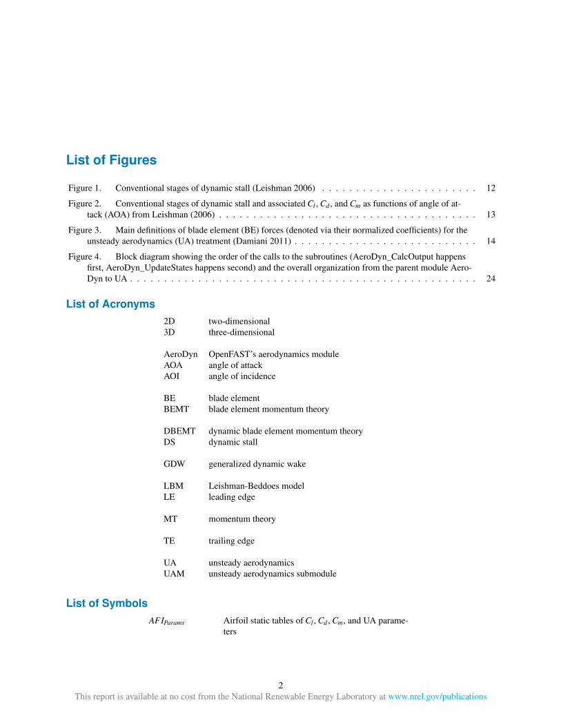
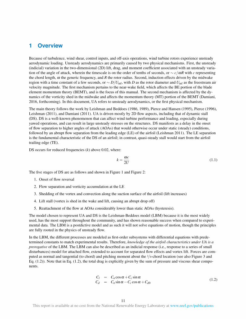
The five stages of DS are as follows and shown in Figure 1 and Figure 2:

1. Onset of flow reversal

2. Flow separation and vorticity accumulation at the LE

3. Shedding of the vortex and convection along the suction surface of the airfoil (lift increases)

4. Lift stall (vortex is shed in the wake and lift, causing an abrupt drop off)

5. Reattachment of the flow at AOAs considerably lower than static AOAs (hysteresis).

The model chosen to represent UA and DS is the Leishman-Beddoes model (LBM) because it is the most widely

used, has the most support throughout the community, and has shown reasonable success when compared to experi-

mental data. The LBM is a postdictive model and as such it will not solve equations of motion, though the principles

are fully rooted in the physics of unsteady flow.

In the LBM, the different processes are modeled as first-order subsystems with differential equations with prede-

termined constants to match experimental results. Therefore, knowledge of the airfoil characteristics under UA is a

prerogative of the LBM. The LBM can also be described as an indicial response (i.e., response to a series of small

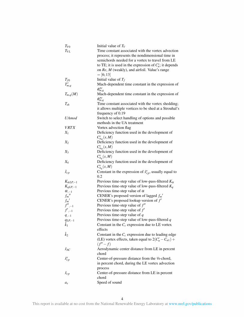
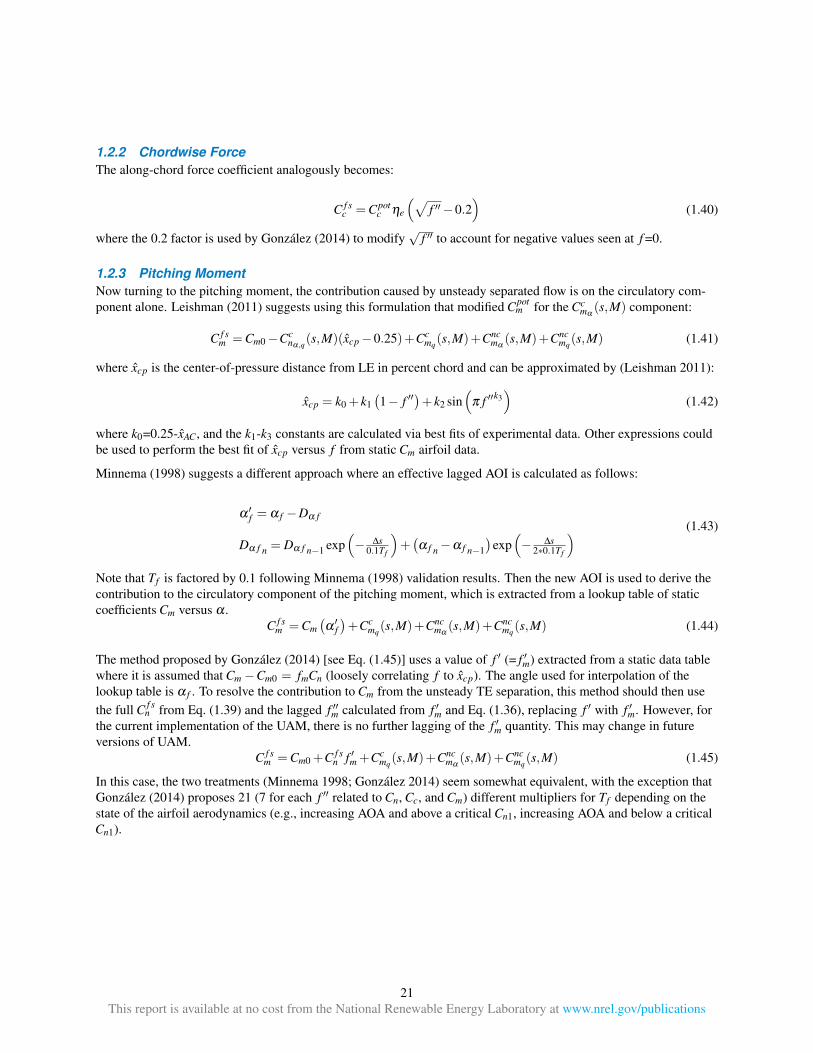
disturbances) model for attached flow, extended to account for separated flow effects and vortex lift. Forces are com-

puted as normal and tangential (to chord) and pitching moment about the

1/ 4 -chord location (see also Figure 3 and

Eq. (1.2)). Note that in Eq. (1.2), the total drag is explicitly given by the sum of pressure and viscous shear compo-

nents.

Cl

= Cn cos α + Cc sin α

Cd

= Cn sin α − Cc cos α + Cd 0

(1.2)

11


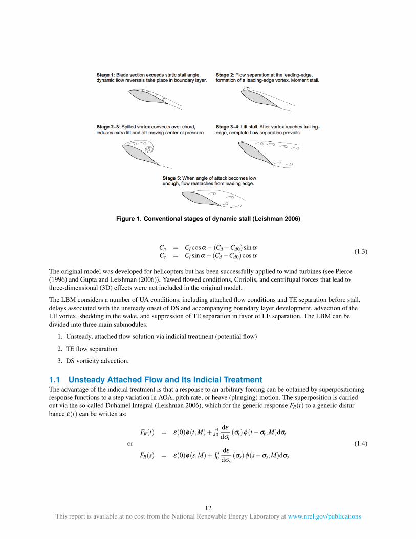
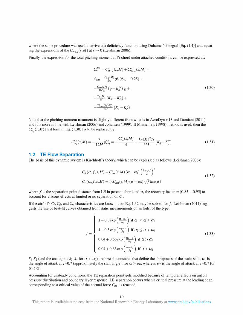
Figure 1. Conventional stages of dynamic stall (Leishman 2006)

Cn

= Cl

cos α +( Cd

− Cd 0) sin α

Cc

= Cl

sin α − ( Cd

− Cd 0) cos α

(1.3)

The original model was developed for helicopters but has been successfully applied to wind turbines (see Pierce

(1996) and Gupta and Leishman (2006)). Yawed flowed conditions, Coriolis, and centrifugal forces that lead to

three-dimensional (3D) effects were not included in the original model.

The LBM considers a number of UA conditions, including attached flow conditions and TE separation before stall,

delays associated with the unsteady onset of DS and accompanying boundary layer development, advection of the

LE vortex, shedding in the wake, and suppression of TE separation in favor of LE separation. The LBM can be

divided into three main submodules:

1. Unsteady, attached flow solution via indicial treatment (potential flow)

2. TE flow separation

3. DS vorticity advection.

1.1 Unsteady Attached Flow and Its Indicial Treatment

The advantage of the indicial treatment is that a response to an arbitrary forcing can be obtained by superpositioning

response functions to a step variation in AOA, pitch rate, or heave (plunging) motion. The superposition is carried

out via the so-called Duhamel Integral (Leishman 2006), which for the generic response FR( t ) to a generic distur-

bance ε ( t ) can be written as:

FR( t ) = ε ( 0 ) φ ( t , M )+

∫ t

0

d ε

d σt

( σt) φ ( t − σt

, M ) d σt

or

FR( s ) = ε ( 0 ) φ ( s , M )+

∫ s

0

d ε

d σs

( σs) φ ( s − σs

, M ) d σs

(1.4)

12


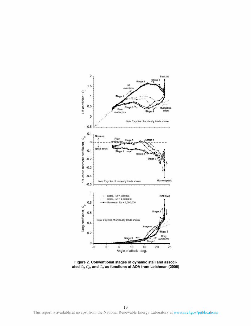
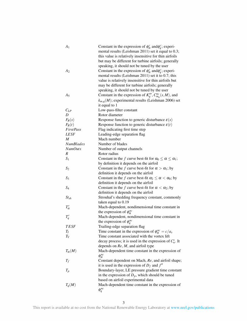
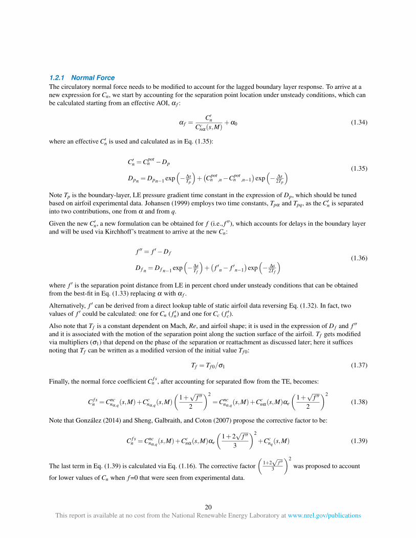
Figure 2. Conventional stages of dynamic stall and associ-

ated Cl , Cd , and Cm

as functions of AOA from Leishman (2006)

13


Figure 3. Main definitions of BE forces (denoted via their nor-

malized coefficients) for the UA treatment (Damiani 2011)

where t is time, M is the Mach number, σt

and σs

are generic integrand coordinates, and s is the nondimensional

distance, defined as:

s =

2

c

∫ t

0

U ( t ) dt (1.5a)

∆ s =

2

cU ( t ) ∆ t (1.5b)

where the airfoil half chord ( c / 2) was taken as the nondimensionalizing factor, and U is the air velocity magnitude

relative to the airfoil.

The indicial functions ( φ ( s , M ) ) are surmised into two components: the first is related to the noncirculatory (super-

script ‘nc’) loading (piston theory and acoustic wave theory), and the second (superscript ‘c’) originates from the

development of circulation about the airfoil. The noncirculatory part depends not only on the instantaneous airfoil

motion, but on the time history of the prior motion. The circulatory response can be calculated via the ‘lumped ap-

proach’, wherein the effects of step changes in AOA ( α ), pitch rate, heave motion, and so on are combined into an

effective AOA at the

3/ 4 -chord station.

1.1.1 Normal Force

The normal force coefficient response to a step change in nondimensional pitch rate q and a step change in AOA can

be written as a function of the indicial functions as shown in Eq. (1.6):

Cn α , q( s , M ) = Cn α( s , M )+ Cnq( s , M ) = Cn α( M ) α + Cnq( s , M ) q

Cn α( s , M ) =

4

M

φ nc

α

+

Cn α( M )

βM

φ c

α

Cnq( s , M ) =

1

M

φ ncq

+

Cn α( M )

2 βM

φ cq

(1.6)

where βM

is the Prandtl-Glauert compressibility correction factor

√

1 − M2, and Cn α( M ) is the slope of the 2D

normal coefficient curve, similar to Cl α .

14


The nondimensional pitch rate q is given by:

q =

˙ α c

U

'

K α nc

U

with : K α n

=

αn

− αn − 1

∆ t

(1.7)

where the subscript ‘n’ denotes the n-th time step.

For small ∆ t ’s, the finite difference K α

can be subjected to significant numerical noise. To smooth out the terms

associated with time derivatives, a low-pass-filter is introduced. The filter is applied to α , q , and its derivative Kq

(which is used later) as defined in Eq. (1.8):

αLPn

= CLP

αLPn − 1

+( 1 − CLP) αn

qn

=

(

αLPn

− αLPn − 1

)c

Un∆ t

qLPn

= CLPqLPn − 1 +( 1 − CLP) qn

K α LPn

=

qLPnUn

c

Kqn

=

qn

− qn − 1

∆ t

KqLPn

= CLPKqLPn − 1

+( 1 − CLP) Kqn

with :

CLP

= e− 2 π ∆ t ζLP

(1.8)

and where αLPn

is the low-pass-filtered value of α , qLP

is the low-pass-filtered value of q , K α LP

is the modified value

of K α

due to filtered α and q , Kq

is the backward finite difference of q , KqLP

is the low-pass-filtered value of Kq, CLP

is the low-pass-filter constant, and ζLP

is the low-pass-filter frequency cutoff ( − 3dB).

From here on, the ‘LP’ subscript is dropped with the understanding that quantities such as α , K α , q , and Kq

denote

the respective filtered quantities αLPn , K α LP, qLP, and KqLP

as defined in Eq. (1.8).

The indicial responses can then be approximated as in Eq. (1.9) (Leishman and Beddoes 1989; Johansen 1999):

φ c

α

= φ cq

= 1 − A1 exp

(− b1

β 2Ms)

− A2 exp

(− b2

β 2Ms)

φ nc

α

= exp

(

−

s

T

′

α

)

φ ncq

= exp

(

−

s

T

′q

)

(1.9)

where A1, A2, b1, and b2

are constants that were tuned from experimental results on oscillating airfoils in the wind

tunnel, and that are relatively insensitive to the airfoil shapes, at least for thin airfoils such as those used in rotorcraft

(see ‘List of Symbols‘ at the beginning of this document); the time constants T

′

α

and T

′q

are defined below.

By making use of exact results for short times 0 ≤ s ≤ 2 M / ( M + 1 ) (Lomax et al. 1952), Leishman (2011) shows

that:

T α( M ) = 0 . 75

c

2 U T

′

α

= 0 . 75

c

2 MasT

′

α

= 0 . 75 k α( M ) TI

Tq( M ) = 0 . 75

c

2 U T

′q

= 0 . 75

c

2 MasT

′q

= 0 . 75 kq( M ) TI

(1.10)

15


where:

k α( M ) =[( 1 − M )+ Cn α( M ) M2

βM ( A1b1 + A2b2)]− 1

(1.11a)

kq( M ) =[( 1 − M )+ Cn α( M ) M2

βM ( A1b1 + A2b2)]− 1

(1.11b)

TI

=

c

as

(1.11c)

where as

is the speed of sound.

Note that Leishman (2011) recommends the use of the factor 0.75 for T α( M ) and Tq( M ) to account for three-

dimensional effects not included in piston theory.

For the circulatory component of the aerodynamic force response, the lumped approach can lead to a direct solution

of Ccn α , q( s , M ) . Considering the circulatory part Cc

n α( s , M ) of Eq. (1.6) for the response to the step in α , it can be

written:

Ccn α( s , M ) =

∫ s

s0

Cn α ( M )

βM

φ c

α

α ( s ) d s ' Ccn α( s , M ) ∆ α

where Ccn α( s , M ) =

Cn α ( M )

βM

(1.12)

By using Eq. (1.4) with φ ( s , M ) replaced by φ c

α

and ε ( s ) by α , Eq. (1.12) rewrites:

Cc

n α , q( s , M ) = Cc

n α( s , M )

[

α ( s0) φc

α( s )+

∫ s

s0

d α

d σs

( σs) φc

α( s − σs

, M ) d σs

]

= Cc

n α( s , M ) αe

(1.13)

where αe

is an effective angle of attack at

3/ 4 -chord accounting for a step variation in α , pitching rate, heave, and

velocity (lumped approach). By applying the first of Eq. (1.9), and setting s0

= 0, Eq. (1.13) can be simplified to

arrive at an expression for αe

at the n-th time step, (i.e., αen ):

αen( s , M ) = ( αn

− α0) − X1n( ∆ s ) − X2n( ∆ s ) (1.14)

where the

∫ s

s0[ ... ] d σs

was numerically integrated. By carrying out the algebra, a recursive expression for X1

and X2

can be found:

X1n

= X1n − 1 exp

(− b1

β 2M∆ s

)+ A1 exp

(− b1

β 2M

∆ s

2

)

∆ αn

X2n

= X2n − 1 exp

(− b2

β 2M∆ s

)+ A2 exp

(− b2

β 2M

∆ s

2

)

∆ αn

(1.15)

Note that α0

was introduced into Eq. (1.14) because αe

is an effective angle of incidence (AOI) and not AOA.

Similar to the above development, the circulatory contribution to Ccn α , q( s , M ) from a step change in q can be derived

as:

Cc

nq( s , M ) =

Ccn α( s , M )

2

[ q − X3( ∆ s ) − X4( ∆ s )] (1.16)

with

X3n

= X3n − 1 exp

(− b1

β 2M∆ s

)+ A1 exp

(− b1

β 2M

∆ s

2

)

∆ q

X4n

= X4n − 1 exp

(− b2

β 2M∆ s

)+ A2 exp

(− b2

β 2M

∆ s

2

)

∆ q

(1.16a)

Eqs. (1.16)-(1.16a) are used by González (2014).

16


However, following the original LBM method, the lumped approach can account for any effect to α , including step

changes in q , so Eq. (1.16) is not necessary and is virtually included via Eq. (1.13) and (1.14).

The noncirculatory part cannot be handled via the superposition (lumped approach); therefore, the contribution from

step changes in α and q need to be kept separate:

Cnc

n α , q( s , M ) = Cnc

n α( s , M )+ Cnc

nq ( s , M ) (1.17)

Now, using Duhamel’s integral (1.4) on the noncirculatory component Cncn α( s , M ) [see Eq. (1.17)] with the φ nc

α

from

Eq. (1.9), the following can be arrived at:

Cncn α( s , M ) =

4 T α ( M )

M

( K α

− K

′

α)

K

′

α n

= K

′

α n − 1 exp

(

−

∆ t

T α ( M )

)

+( K α n

− K α n − 1) exp

(

−

∆ t

2 T α ( M )

)

(1.18)

Note that in Eq. (1.18), K

′

α

is the deficiency function for Cncn α( s , M ) .

For Cncnq ( s , M ) , an analogous procedure leads to:

Cncnq ( s , M ) = −Tq( M )

M

(

Kqn

− K

′qn

)

K

′qn

= K

′qn − 1 exp

(

−

∆ t

Tq( M )

)

+

(Kqn

− Kqn − 1

)exp

(

−

∆ t

2 Tq( M )

)

(1.19)

So finally, the expression for the total normal force under attached conditions Cpotn

can be expressed as:

Cpotn

= Cpot , cn

+ Cpot , ncn

Cpotn

= Ccn α , q( s , M )+ Cnc

n α , q( s , M ) = Ccn α( s , M ) αe +

4 T α ( M )

M

( K α n

− K

′

α n)+

Tq( M )

M

(Kq

− K

′q

)

with

Cpot , cn

= Ccn α , q( s , M ) = Cc

n α( s , M ) αe

Cpot , ncn

= Cncn α , q( s , M ) =

4 T α ( M )

M

( K α

− K

′

α)+

Tq( M )

M

(Kq

− K

′q

)

(1.20)

1.1.2 Chordwise Force

The chordwise force can be written as in Eq. (1.21) from Leishman (2011):

Cpot

c

= Cpot , c

n

tan ( αe + α0) (1.21)

In potential flow, D’Alambert’s paradox leads to the absence of drag; therefore, from Eq. (1.3), Cl

cos α = Cn

and

Cc

= Cl

sin α , which bring forth Eq. (1.21). Because αe

is a virtual angle of incidence at

3/ 4 -chord, we needed to add

the α0. Because this drag treatment has roots only in the circulatory lift derivation, the noncirculatory part is dropped

as shown in Eq. (1.21).

17


1.1.3 Pitching Moment

Analogous to the normal force treatment, the pitching moment coefficient about the

1/ 4 -chord can be derived via

indicial response as shown in Eq. (1.22):

Cm α , q( s , M ) = Cm α( s , M )+ Cmq( s , M ) = Cm α

α + Cmq( s , M ) q

Cm α( s , M ) = −

1

M

φ ncm , α

−

Cn α( M )

βM

φ c

α

( ˆ xAC

− 0 . 25 )+ Cm 0

Cmq( s , M ) = −

7

12 M

φ ncm , q

−

Cn α( M )

16 βM

φ cm , q

(1.22)

where ˆ xAC

is the aerodynamic center distance from LE in percent chord, Cm 0

(the 2D pitching moment coefficient

at 0-lift, positive if nose up) is positive if it causes a pitch up of the airfoil, as seen in Figure 3. Also note that the

circulatory component of the pitching moment response to a step change in α is a function of the Ccn α( s , M ) .

The indicial response can be approximated [see also Eq. (1.9)] as:

φnc

m , q

= exp

(

−

s

T

′m , q

)

(1.23)

Analogous expressions can be found for φ cm , q

and φ ncm , α , but they are not shown here because further simplified ex-

pressions will be derived below. In Eq. (1.23), T

′m , q

is the Mach-dependent time constant in the expression of φ ncm , q,

whose expression can be derived in a similar fashion to those of the constants in Eq. (1.10):

Tm , q( M ) =

c

2 U

T

′

m , q

=

c

2 MasT

′

m , q

= km , q( M ) TI

(1.24)

Following Johansen (1999), the circulatory component Ccmq( s , M ) can be written as:

Cc

mq( s , M ) = −Cn α( M )

16 βM

(q − K

′′′

q

) c

U

(1.25)

where:

K

′′′

q n

= K

′′′

q n − 1 exp

(− b5

βM2∆ s)+ A5∆ qn exp

(

− b5

βM2

∆ s

2

)

(1.26)

with A5

and b5

constants set to 1 and 5, respectively, from experimental results (Leishman 2006).

The noncirculatory component of the pitching moment response to the step change in α , Cncm α

( s , M ) , writes (Leish-

man and Beddoes 1986; Johansen 1999):

Cnc

m α( s , M ) = −

1

M

φnc

m , α

= −Cnc

n α( s , M )

4

(1.27)

which implies

φnc

m , α

= φnc

α

(1.28)

The other noncirculatory component, Cncmq( s , M ) , writes (Leishman 2006):

Cncmq( s , M ) = −

7

12 M

φ ncm , q

= − 7 km , q( M )2TI

12 M

(Kq

− K

′′q

)

with:

km , q( M ) =

7

15 ( 1 − M )+ 1 . 5 Cn α ( M ) A5b5

βMM2

K

′′q n

= K

′′q n − 1 exp

(

−

∆ t

km , q( M )2TI

)

+

(Kqn

− Kqn − 1

)exp

(

−

∆ t

2 km , q( M )2TI

)

(1.29)

18


where the same procedure was used to arrive at a deficiency function using Duhamel’s integral [Eq. (1.4)] and equat-

ing the expressions of the Cm α , q( s , M ) at s → 0 (Leishman 2006).

Finally, the expression for the total pitching moment at

1/ 4 -chord under attached conditions can be expressed as:

Cpotm

= Ccm α , q( s , M )+ Cnc

m α , q( s , M ) =

Cm 0

−

Cn α ( M )

βM

φ c

α

( ˆ xAC

− 0 . 25 )+

−Cn α ( M )

16 βM

(q − K

′′′q

) c

U +

−T α ( M )

M

( K α

− K

′

α)+

− 7 km , q( M )2TI

12 M

(Kq

− K

′′q

)

(1.30)

Note that the pitching moment treatment is slightly different from what is in AeroDyn v.13 and Damiani (2011)

and it is more in line with Leishman (2006) and Johansen (1999). If Minnema’s (1998) method is used, then the

Cncmq( s , M ) [last term in Eq. (1.30)] is to be replaced by:

Cnc

mq( s , M ) = −

7

12 M

φnc

m , q

= −Cnc

nq ( s , M )

4

−

k α( M )2TI

3 M

(Kq

− K

′′

q

)

(1.31)

1.2 TE Flow Separation

The basis of this dynamic system is Kirchhoff’s theory, which can be expressed as follows (Leishman 2006):

Cn ( α , f , s , M ) = Ccn α( s , M )( α − α0)

(1 +√

f

2

)2

Cc ( α , f , s , M ) = ηeCcn α( s , M )( α − α0)

√

f tan ( α )

(1.32)

where f is the separation point distance from LE in percent chord and ηe

the recovery factor ' [ 0 . 85 − 0 . 95 ] to

account for viscous effects at limited or no separation on Cc.

If the airfoil’s Cl , Cd , and Cm

characteristics are known, then Eq. 1.32 may be solved for f . Leishman (2011) sug-

gests the use of best-fit curves obtained from static measurements on airfoils, of the type:

f =

1 − 0 . 3exp

(

α − α1

S1

)

, if α0

≤ α ≤ α1

1 − 0 . 3exp

(

α2

− α

S3

)

, if α2

≤ α < α0

0 . 04 + 0 . 66exp

(

α1

− α

S2

)

, if α > α1

0 . 04 + 0 . 66exp

(

α − α2

S4

)

, if α < α2

(1.33)

S1- S2

(and the analogous S3- S4

for α < α0) are best-fit constants that define the abruptness of the static stall. α1

is

the angle of attack at f =0.7 (approximately the stall angle), for α ≥ α0, whereas α2

is the angle of attack at f =0.7 for

α < α0.

Accounting for unsteady conditions, the TE separation point gets modified because of temporal effects on airfoil

pressure distribution and boundary layer response. LE separation occurs when a critical pressure at the leading edge,

corresponding to a critical value of the normal force Cn 1, is reached.

19


1.2.1 Normal Force

The circulatory normal force needs to be modified to account for the lagged boundary layer response. To arrive at a

new expression for Cn, we start by accounting for the separation point location under unsteady conditions, which can

be calculated starting from an effective AOI, α f :

α f

=

C

′n

Ccn α( s , M )

+ α0

(1.34)

where an effective C

′n

is used and calculated as in Eq. (1.35):

C

′n

= Cpotn

− Dp

Dpn

= Dpn − 1 exp

(

−

∆ s

Tp

)

+

(Cpot

n , n

− Cpotn , n − 1

)exp

(

−

∆ s

2 Tp

)

(1.35)

Note Tp

is the boundary-layer, LE pressure gradient time constant in the expression of Dp, which should be tuned

based on airfoil experimental data. Johansen (1999) employs two time constants, Tp α

and Tpq, as the C

′n

is separated

into two contributions, one from α and from q .

Given the new C

′n, a new formulation can be obtained for f (i.e., f

′′), which accounts for delays in the boundary layer

and will be used via Kirchhoff’s treatment to arrive at the new Cn:

f

′′ = f

′ − D f

D f n

= D f n − 1 exp

(

−

∆ s

Tf

)

+

(f

′n

− f

′n − 1

)exp

(

−

∆ s

2 Tf

)

(1.36)

where f

′ is the separation point distance from LE in percent chord under unsteady conditions that can be obtained

from the best-fit in Eq. (1.33) replacing α with α f .

Alternatively, f

′ can be derived from a direct lookup table of static airfoil data reversing Eq. (1.32). In fact, two

values of f

′ could be calculated: one for Cn

( f

′n) and one for Cc

( f

′c).

Also note that Tf

is a constant dependent on Mach, Re , and airfoil shape; it is used in the expression of D f

and f

′′

and it is associated with the motion of the separation point along the suction surface of the airfoil. Tf

gets modified

via multipliers ( σ1) that depend on the phase of the separation or reattachment as discussed later; here it suffices

noting that Tf

can be written as a modified version of the initial value Tf 0:

Tf

= Tf 0

/ σ1

(1.37)

Finally, the normal force coefficient C f sn

, after accounting for separated flow from the TE, becomes:

C f s

n

= Cnc

n α , q( s , M )+ Cc

n α , q( s , M )

(1 +

√

f

′′

2

)2

= Cnc

n α , q( s , M )+ Cc

n α( s , M ) αe

(1 +

√

f

′′

2

)2

(1.38)

Note that González (2014) and Sheng, Galbraith, and Coton (2007) propose the corrective factor to be:

C f s

n

= Cnc

n α , q( s , M )+ Cc

n α( s , M ) αe

(1 + 2

√

f

′′

3

)2

+ Cc

nq( s , M ) (1.39)

The last term in Eq. (1.39) is calculated via Eq. (1.16). The corrective factor

(

1 + 2√

f

′′

3

)2

was proposed to account

for lower values of Cn

when f =0 that were seen from experimental data.

20



The along-chord force coefficient analogously becomes:

C f s

c

= Cpot

c

ηe

(√

f

′′ − 0 . 2

)

(1.40)

where the 0.2 factor is used by González (2014) to modify

√

f

′′ to account for negative values seen at f =0.


Now turning to the pitching moment, the contribution caused by unsteady separated flow is on the circulatory com-

ponent alone. Leishman (2011) suggests using this formulation that modified Cpotm

for the Ccm α

( s , M ) component:

C f s

m

= Cm 0

− Cc

n α , q( s , M )( ˆ xcp

− 0 . 25 )+ Cc

mq( s , M )+ Cnc

m α( s , M )+ Cnc

mq( s , M ) (1.41)

where ˆ xcp

is the center-of-pressure distance from LE in percent chord and can be approximated by (Leishman 2011):

ˆ xcp

= k0 + k1

(1 − f

′′

)+ k2 sin

(

π f

′′k3

)

(1.42)

where k0=0.25- ˆ xAC, and the k1- k3

constants are calculated via best fits of experimental data. Other expressions could

be used to perform the best fit of ˆ xcp

versus f from static Cm

airfoil data.

Minnema (1998) suggests a different approach where an effective lagged AOI is calculated as follows:

α

′

f

= α f

− D α f

D α f n

= D α f n − 1 exp

(

−

∆ s

0 . 1 Tf

)

+

(

α f n

− α f n − 1

)exp

(

−

∆ s

2 ∗ 0 . 1 Tf

)

(1.43)

Note that Tf

is factored by 0.1 following Minnema (1998) validation results. Then the new AOI is used to derive the

contribution to the circulatory component of the pitching moment, which is extracted from a lookup table of static

coefficients Cm

versus α .

C f s

m

= Cm

(

α

′

f

)+ Cc

mq( s , M )+ Cnc

m α( s , M )+ Cnc

mq( s , M ) (1.44)

The method proposed by González (2014) [see Eq. (1.45)] uses a value of f

′ (= f

′m) extracted from a static data table

where it is assumed that Cm

− Cm 0

= fmCn

(loosely correlating f to ˆ xcp). The angle used for interpolation of the

lookup table is α f . To resolve the contribution to Cm

from the unsteady TE separation, this method should then use

the full C f sn

from Eq. (1.39) and the lagged f

′′m

calculated from f

′m

and Eq. (1.36), replacing f

′ with f

′m. However, for

the current implementation of the UAM, there is no further lagging of the f

′m

quantity. This may change in future

versions of UAM.

C f s

m

= Cm 0 + C f s

n

f

′

m + Cc

mq( s , M )+ Cnc

m α( s , M )+ Cnc

mq( s , M ) (1.45)

In this case, the two treatments (Minnema 1998; González 2014) seem somewhat equivalent, with the exception that

González (2014) proposes 21 (7 for each f

′′ related to Cn, Cc, and Cm) different multipliers for Tf

depending on the

state of the airfoil aerodynamics (e.g., increasing AOA and above a critical Cn 1, increasing AOA and below a critical

Cn 1).

21


1.3 Dynamic Stall

1.3.1 Normal Force

During DS, there is shear layer roll up at the LE with associated vortex formation, and vortex travel over the upper

surface of the airfoil that will be subsequently shed in the wake. The main condition to be met for the shear layer roll

up is:

C

′n

> Cn 1

for α ≥ α0

C

′n

< Cn 2

for α < α0

(1.46)

The normal force coefficient contribution from the additional lift associated with the low-pressure LE vortex can be

written as (Leishman 2011):

Cv

n , n

= Cv

n , n − 1 exp

(

−∆ s

TV

)

+( CV n

− CV n − 1) exp

(

−

∆ s

2 TV

)

(1.47)

TV

is the time constant associated with the vortex lift decay process and it depends on Re , M , and airfoil type. Note

that the Cvn

contribution is not allowed to have a sign opposite to that of C f sn

.

TV

gets modified via a multiplier σ3

to account for various stages of the process, as discussed later, but here it suf-

fices to say that:

TV

= TV 0

/ σ3

(1.48)

CV

represents the contribution to the normal force coefficient due to accumulated vorticity in the LE vortex. CV

is

modeled proportionally to the difference between the attached and separated circulatory contributions to Cn:

CV

= Cc

n α , q( s , M ) − Cc

n α , q( s , M )

(1 +

√

f

′′

2

)2

= Cc

n α( s , M ) αe

(

1 −

1 +

√

f

′′

2

)2

(1.49)

If the method proposed by González (2014) is used, then CV

can be written as:

CV

= Cc

n α( s , M ) αe

(

1 −

1 + 2√

f

′′

3

)2

(1.50)

The position of the LE vortex along the chordwise direction is tracked via a nondimensional time variable, τV ,

defined in Eq. (1.51):

τV

= t2 U

c

(1.51)

If τV =0, the vortex is at the LE; if τV = TV L, the vortex is at the TE.

If τV

> TV L

and if α f

is not moving away from stall (i.e., [( α f

− α0) ∗ ( α f n

− α f n − 1)] > 0) , then the vorticity is no

longer allowed to accumulate, in which case Eq. (1.47) can be rewritten as:

Cvn , n

= Cvn , n − 1 exp

(

−

∆ s

TV 0

/ σ3

)

with σ3

= 2

(1.52)

where the decay of the normal force (due to vorticity at the LE) is accelerated at twice the original rate and no further

accretion of vorticity is allowed. Eq. (1.52) should also be used when conditions in Eq. (1.46) are not met. Note that

TV L

represents the time constant associated with the vortex advection process; it represents the nondimensional time

in semichords needed for a vortex to travel from LE to TE; it is used in the expression of Cvn; it depends on Re , M

(weakly), and airfoil. Value’s range = [ 6;13 ] .

Finally, the total normal force can be written as:

Cn

= C f s

n

+ Cv

n

= Cc

n α( s , M ) αe

(1 +

√

f

′′

2

)2

+ Cnc

n α , q( s , M )+ Cv

n

(1.53)

22


Again, if González’s (2014) method is used, then the correction factor for the separated flow treatment is slightly

modified as in Eq. (1.50), for example:

Cn

= C f s

n

+ Cv

n

= Cc

n α( s , M ) αe

(1 + 2

√

f

′′

3

)2

+ Cnc

n α , q( s , M )+ Cv

n

(1.53b)

Note that multiple vortices can be shed at a given shedding frequency corresponding to:

Tsh

= 21 − f

′′

Stsh

(1.54)

Therefore, τV

is reset to 0 if τV

= TV L + Tsh.


The along-chord force coefficient gets modified by the presence of the LE vortex as in Pierce (1996):

Cc

= C f s

c

+ Cv

n tan ( αe)

(

1 −

τV

TV L

)

(1.55)

Note that in the current release of UA, the tan ( αe) ' αe

approximation is made. This may be changed after testing in

future releases.

González (2014) does not contain the vortex contribution to Cc

based on experimental validation:

Cc

= C f s

c

(1.55b)

The original Leishman and Beddoes (1989) model had Cc

written as:

Cc

=

{

ηeCpotc

√

f

′′ sin ( αe + α0) , C

′n

≤ Cn 1

k̂1 + Cpotc

√

f

′′ f

′′ k̂2 sin ( αe + α0) , C

′n

> Cn 1

(1.56a)

with : k̂2

= 2 ( C

′

n

− Cn 1)+ f

′′ − f (1.56b)

where k̂1

is a constant required to fit the Cc

curve under static conditions for 2D airfoils.


Leishman (2011) offers a form for the ˆ xvcp, which is the center-of-pressure distance from the

1/ 4 -chord, in percent

chord, during the LE vortex advection process:

Cvm

= − ˆ xvcpCv

n

ˆ xvcp( τV ) =

¯̄ xcp

(

1 − cos

(

π τV

TV L

)) (1.57)

where

¯̄ xcp

is a constant in the expression of ˆ xvcp, usually equal to 0.2.

Finally, the expression for the total pitching moment can be written as:

Cm

= Cm 0

− Cc

n α , q( s , M )( ˆ xcp

− 0 . 25 )+ Cc

mq( s , M )+ Cnc

m α( s , M )+ Cnc

mq( s , M )+ Cv

m

(1.58)

If Minnema’s (1998) approach is used, then Eq. (1.58) can be rewritten as:

Cm

= Cm

(

α

′

f

)+ Cc

mq( s , M )+ Cnc

m α( s , M )+ Cnc

mq( s , M )+ Cv

m

(1.59)

and if González’s (2014) treatment is used, the total moment becomes:

Cm

= Cn

fm

′′+ Cc

mq( s , M )+ Cnc

m α( s , M )+ Cnc

mq( s , M )+ Cv

m

(1.60)

23


2 Inputs, Outputs, Parameters, States, and Implementation of UA

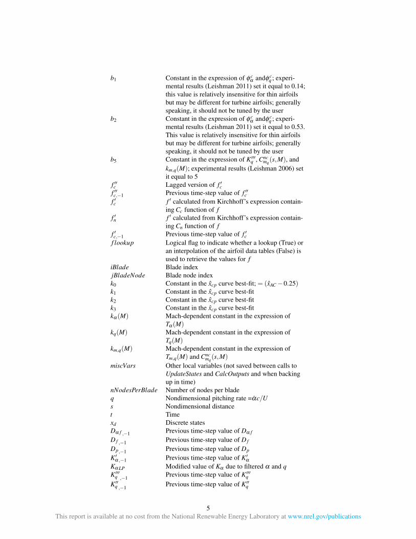
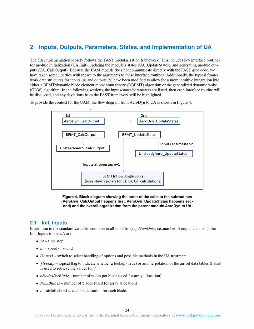
The UA implementation loosely follows the FAST modularization framework. This includes key interface routines

for module initialization (UA_Init), updating the module’s states (UA_UpdateStates), and generating module out-

puts (UA_CalcOutput). Because the UAM module does not communicate directly with the FAST glue code, we

have taken some liberties with regard to the arguments to these interface routines. Additionally, the typical frame-

work data structures for inputs (u) and outputs (y) have been modified to allow for a more intuitive integration into

either a BEMT/dynamic blade element momentum theory (DBEMT) algorithm or the generalized dynamic wake

(GDW) algorithm. In the following sections, the inputs/states/parameters are listed, then each interface routine will

be discussed, and any deviations from the FAST framework will be highlighted.

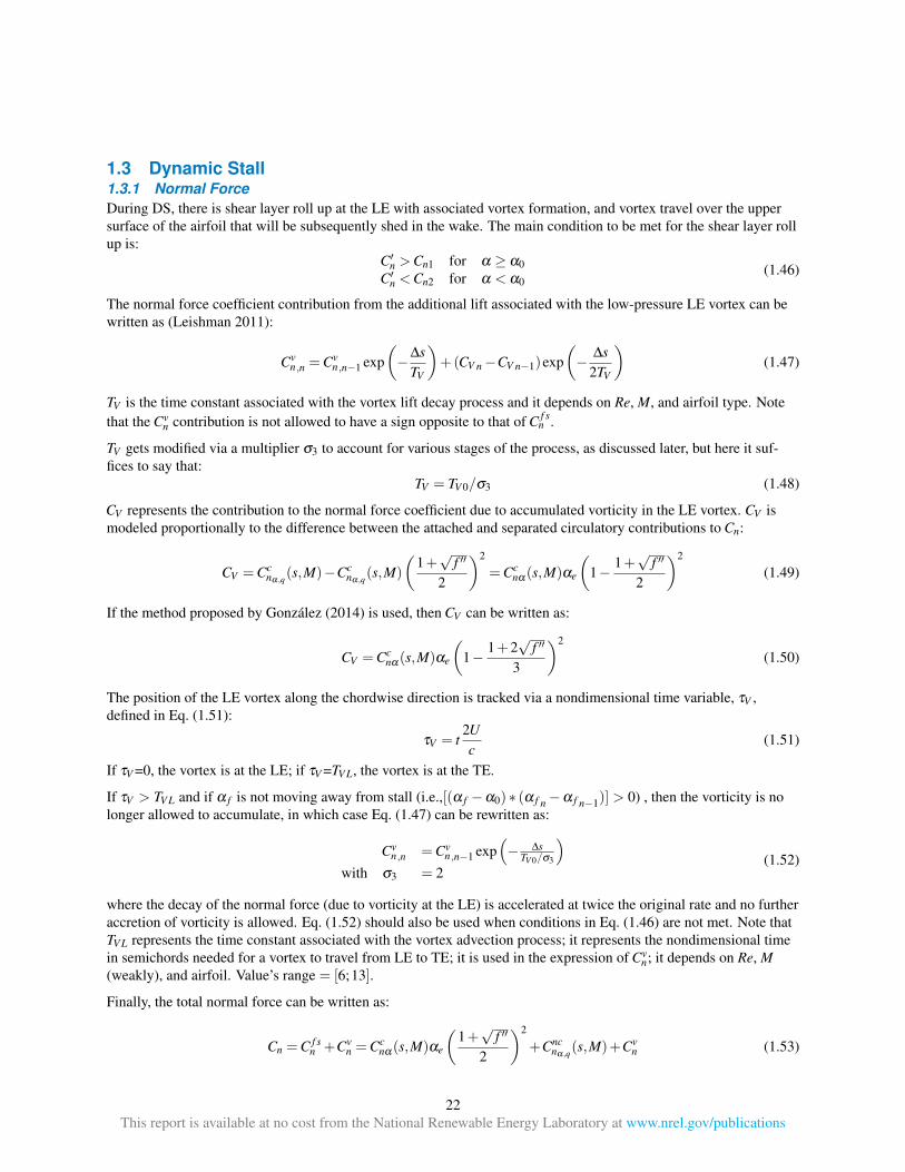
To provide the context for the UAM, the flow diagram from AeroDyn to UA is shown in Figure 4.

Figure 4. Block diagram showing the order of the calls to the subroutines

(AeroDyn_CalcOutput happens first, AeroDyn_UpdateStates happens sec-

ond) and the overall organization from the parent module AeroDyn to UA

2.1 Init_Inputs

In addition to the standard variables common to all modules (e.g., NumOuts , i.e.,number of output channels), the

Init_Inputs to the UA are:

• ∆ t – time step

• as

– speed of sound

• UAmod – switch to select handling of options and possible methods in the UA treatment

• f lookup – logical flag to indicate whether a lookup (True) or an interpolation of the airfoil data tables (False)

is used to retrieve the values for f

• nNodesPerBlade – number of nodes per blade (used for array allocation)

• NumBlades – number of blades (used for array allocation)

• c – airfoil chord at each blade station for each blade.

24


2.2 Inputs u

The inputs to the UA are:

• α

• U

• Re .

Note: these are for a given node (within a given blade).

2.3 Outputs y

The outputs from the UA are:

• Cn

• Cc

• Cm

• Cl

• Cd

(this includes the viscous shear component Cd 0).

Note: these are for a given node (within a given blade).

2.4 States xd

The states for the UA are:

Discrete states :

• α , − 1

– previous time-step value of α

• αLP , − 1

– previous time-step value of low-pass-filtered α

• α f , − 1

– previous time-step value of α f

• q, − 1

– previous time-step value of q

• qLP , − 1

– previous time-step value of low-pass-filtered q

• K α LP , − 1

– previous time-step value of low-pass-filtered K α

• KqLP , − 1

– previous time-step value of low-pass-filtered Kq

• X1 , − 1

– previous time-step value of X1

• X2 , − 1


• X3 , − 1


• X4 , − 1


• K

′

α , − 1

– previous time-step value of K

′

α

• K

′q , − 1


′q

• K

′′q , − 1


′′q

• K

′′′q , − 1


′′′q

• Dp , − 1

– previous time-step value of Dp

25


• D f , − 1

– previous time-step value of D f

• D fc

, − 1

– previous time-step value of D fc

( D fc

is the deficiency function for f

′c

analgous to D f )

• Cpotn , − 1

– previous time-step value of Cpotn

• f

′

, − 1

– previous time-step value of f

′

• f

′

c , − 1


′c

• f

′′

, − 1


′′

• f

′′

c , − 1


′′c

( f

′′c

is the lagged version of f

′c)

• τV

– time variable that tracks the travel of the LE vortex over the airfoil suction surface. It is made dimension-

less via the semichord: τV

= t ∗ 2 U / c . If less than 2 TV L, it renders the logical flag V RT X =True; if less than

TV L, then the vortex is still on the airfoil

• τV , − 1

– previous time-step value of τV

• Cvn , − 1

– previous time-step value of Cvn

• CV , − 1

– previous time-step value of CV

• D α f , − 1

– previous time-step value of D α f

The FAST 8 framework does not allow logical or discontinuous variables within states. For this reason, the following

are declared as either Other States or miscVars (other local variables (not saved between calls to UpdateStates and

CalcOutputs and when backing up in time)).

Other states :

• σ1

– generic multiplier for Tf

• σ3

– generic multiplier for TV

miscVars :

• iBlade – blade index

• jBladeNode – blade node index

• T ESF – trailing-edge separation flag

• LESF – leading-edge separation flag

• V RT X – vortex advection flag

• FirstPass - flag indicating first time step

Note that, in contrast to inputs and outputs, the states must be tracked by the UA module; therefore, they are a 2-D

array (per blade, per node).

2.5 Parameters p

The parameters for the UA are:

• ∆ t – time step

• c – chord length

• UAmod – switch to select handling of options and possible methods in the UA treatment

• as

– speed of sound

26


• f lookup – logical flag to indicate whether a lookup (True) or an interpolation of the airfoil data tables (False)

is used to retrieve the values for f

• ζLP

– low-pass-filter frequency cutoff ( − 3dB)

• nNodesPerBlade – number of nodes per blade

• NumBlades – number of blades

An airfoil data structure ( AFIParams) is passed directly to the UAM framework routines and is indexed to the airfoil

of interest. AFIParams

contains airfoil-specific quantities

, i.e., parameters and constants for the UA, alhtough it is not

formally a parameter of the FAST 8 framework:

• α0, α1, α2, Cn α( M ) , Cn 1, Cn 2, ηe, Cd 0, Cm 0,

¯̄ xcp, Stsh

• A1, b1, A2, b2, A5, b5

• S1, S2, S3, S4

• Tp

(fairly independent of airfoil type)

• Tf 0, TV 0, TV L

• k0, k1, k2, k3

• k̂1.

These parameters were introduced in this manual and their meanings are provided in the list of symbols at the begin-

ning of the document.

2.6 UA Implementation

2.6.1 UA_Init Routine

This routine allocates the module’s data structures and sets the nontime-varying parameters (copies them from the

initialization input data section).

2.6.2 UA_UpdateStates Routine

The typical list of arguments to UA_UpdateStates gets augmented to pass indices to the blade and blade node of

interest and the structure AFIParams, which contains the airfoil data.

The model is of the parsimonious, open-loop, Kelvin-chain kind. Outputs of each subsystem serve as inputs to the

next subsystem. There are no differential equations to solve. There is no solver per se; for this reason states are

discrete states only (see Section 2.4 for other states).

2.6.2.1 UAmod Logical Flags

The options implemented in the code are selected via the UAmod switch and f lookup flag:

• UAmod =1: closest model to the original Leishman-Beddoes formulation

• UAmod =2: modifications to the original model and simplifications following González (2014)

• UAmod =3: modifications to the original model and simplifications following Pierce (1996) and Minnema

(1998)

• f lookup =True: Eq. (1.33) gets replaced by lookup values for f

′n

f

′c. Note that if UAmod =2 or 3, the flag is

automatically set to True.

In what follows, the modifications to the algorithm for UAmod =2 or 3 are given with respect to the sequence of

equations used for UAmod =1.

27


If UAmod =2, then:

Replace Eq. (1.58) with Eq. (1.60)

Replace Eq. (1.56) with Eq. (1.55b)

Replace Eq. (1.53) with Eq. (1.53b)




Add Eq. (1.16) to Ccn α , q( s , M ) Eq. (1.13).

If UAmod =3, then:



Replace Eq. (1.41) with Eq. (1.43)-(1.44)

Modify Eq. (1.30) with Eq. (1.31).

2.6.2.2 Update Discrete States

For a given set of inputs, (u), and at the current step in time, (t), the Kelvin chain is performed through the following

equations:

• Eq. (1.11c)

• Eq. (1.5b)

• Eq. (1.7)-(1.8)

• Eq. (1.11a) (calculated solely at first time step)

• Eq. (1.11b) (calculated solely at first time step)

• Eq. (1.10)

• Eq. (1.37)

• Eq. (1.48)

• Eq. (1.18)

• Eq. (1.19)

• Eq. (1.17)

• Eq. (1.15)

• Eq. (1.14)

• Eq. (1.13)

• Eq. (1.26)

• Eq. (1.25)

• Eq. (1.20)

• Eq. (1.29)

• Eq. (1.21)

• Eq. (1.35)

• Eq. (1.34)

• Eq. (1.33)

28


• Eq. (1.36)

• Eq. (1.38) [or Eq. (1.39)]

• Eq. (1.49) [or Eq. (1.50)]

• Eq. (1.47) [or Eq. (1.52)].

2.6.2.3 Update Other States

• If C

′n

> Cn 1

( C

′n

< Cn 2

for α < α0), Then:

LESF =True: this means LE separation can occur

Else

LESF =False: this means reattachment can occur

• If f

′′t

< f

′′t − 1, Then:

T ESF =True: this means TE separation is in progress

Else

T ESF =False: this means TE reattachment is in progress

• If 0 < τV

≤ 2 TV L, Then:

V RT X =True: this means vortex advection is in progress

Else

V RT X =False: this means vortex is in wake

• If τV

≥ 1 +

Tsh

TV L

and LESF =True, Then:

τV

is reset to 0.

2.6.2.3.1 Tf

modifications

The following conditional statements operate on a multiplier σ1

that affects Tf , i.e., the actual Tf

is given by

Eq. (1.37):

Tf

= Tf 0

/ σ1

(1.37 revisited)

where Tf 0

is the initial value of Tf ; σ1

= 1 (initialization default value); and ∆ α 0

= α - α0

IF T ESF =True, THEN: (separation)

If K α ∆ α 0

< 0, Then: σ1

= 2 (accelerate separation point movement)

Else If LESF =False, Then: σ1

= 1 (default value, LE separation can occur)

Else If f

′′n − 1

≤ 0 . 7, Then: σ1

= 2 (accelerate separation point movement if separation is occurring)

Else σ1

=1.75 (accelerate separation point movement)

ELSE: (reattachment, this means T ESF =False)

If LESF = False, Then: σ1

= 0.5 (default: slow down reattachment)

If V RT X =True and 0 ≤ τV

≤ TV L, Then: σ1

= 0.25 - No flow reattachment if vortex shedding is in

progress

If K α ∆ α 0

> 0, Then: σ1

= 0.75.

Note the last three conditional statements are separate "ifs."

Although this logic was tested and proved to be effective, the current version of UA uses a simpler version.

2.6.2.3.2 TV

modifications

For TV , an analogous set of conditions is used to set the proper value of the time constant depending on subsystem

stages:

σ3=1 (initialization default value)

If TV L

≤ τV

≤ 2 TV L, Then

29


σ3=3 (postshedding)

If T ESF =False, then:

σ3=4 (accelerate vortex lift decay)

If V RT X =True and 0 ≤ τV

≤ TV L, then:

If K α ∆ α 0

< 0, then σ3=2 (accelerate vortex lift decay)

else σ3=1 (default)

Else if K α ∆ α 0

< 0, then: σ3=4 (vortex lift must decay fast)

If T ESF =False and Kq∆ α 0

< 0, then: σ3=1 (default).

2.6.2.3.3 Update ‘previous time step’ states

After the states are updated to the next time step (t+1) values, the current values at time step, t, are stored into the

(t-1) states.

2.6.3 UA_CalcOutput

This routine determines the outputs, Cn, Cc

(and the transformed versions, Cl

and Cd), and Cm

given the inputs of U ,

α , and Re (currently unused), for a given blade element. Because the routine only generates outputs for a specific

blade element, the FAST framework arguments are augmented to include indices to the blade and blade node of

interest. The routine uses the same Kelvin chain as in UA_UpdateStates; however, the state variables themselves are

not updated during these calculations.

For the first time step, outputs are determined by static lookup tables.

The equations implemented in this routine are the same as in Section 2.6.2.2, plus the following:

• Eq. (1.53)

• Eq. (1.55)

• Eq. (1.2)

• Eq. (1.58).

30


Bibliography

Damiani, R. 2011. Algorithmic Outline of Unsteady Aerodynamics (AeroDyn) Modules . Final Report WE-201103.

NREL Subcontract No. AFT-1-11326-01 under Prime Contract No. DE-AC36-08GO28308. Available upon request

from NREL. Arvada, CO: RRD Engineering, LLC.

— . 2016, forthcoming. The Dynamic Blade Element Momentum Theory For FAST 8 . Technical Report. In Review.

Golden, CO: National Renewable Energy Laboratory (NREL).

González, A. 2014. DYSTOOL Stability Aerodynamic Tool for 2D Airfoil Based on the Beddoes-Leishman Model . In-

forme IN-523/069-en. Wind Energy Department – Fundación CENER-CIEMAT. Avenida Ciudad de la Innovaciion,

7 - 31621-Sarriguren (Navarra) Spain: CENER.

Gupta, S., and J. G. Leishman. 2006. “Dynamic Stall Modeling of the S809 Airfoil and Comparison with Experi-

ments”. Wind Energy 9 (6): 521–547.

Johansen, J. 1999. Unsteady Airfoil Flows with Application to Aeroelastic Stability . Report Risø-R-1116(EN). 98

pages. Roskilde, Denmark: Risø National Laboratory.

Jonkman, J. 2013. “New Modularization Framework for the FAST Wind Turbine CAE Tool”. In Proceedings of the

51st AIAA Aerospace Sciences Meeting . Dallas, TX: AIAA.

Leishman, J. G. 2006. Principles of Helicopter Aerodynamics . 2nd. 826 p. New York, NY: Cambridge University

Press.

— . 2011. Final Report: Assessment of ‘AeroDyn’ Theory Basis Including Unsteady Aerodynamics Modules . NREL

Subcontractor Report LFC-1-11303-01. Prime Contract No. DE-AC36-08GO28308.

Leishman, J. G., and T. S. Beddoes. 1986. “A General Model for Airfoil Unsteady Behavior and Dynamic Stall

Using the Indicial Method”. In Proceedings of the 42nd Annual Forum of the American Helicopter Society , 243–266.

Washington, D.C.: American Helicopter Society.

— . 1989. “A Semi-Empirical Model for Dynamic Stall”. J. of the American Helicopter Society 34 (3): 3–17.

Lomax, H., et al. 1952. Two and Three Dimensional Unsteady Lift Problems in High Speed Flight . Technical Re-

port 1077. NACA.

Minnema, J. E. 1998. Pitching Moment Predictions on Wind Turbine Blades Using the Beddoes-Leishman Model for

Unsteady Aerodynamics and Dynamic Stall . MA thesis, The University of Utah.

Pierce, K. G. 1996. Wind Turbine Load Prediction Using the Beddoes-Leishman Model for Unsteady Aerodynamics

and Dynamic Stall . MA thesis, The University of Utah.

Pierce, K. G., and A. C. Hansen. 1995. “Prediction of Wind Turbine Rotor Loads Using the Beddoes-Leishman

Model for Dynamic Stall”. J. of Solar Energy Engineering 117:200–204.

Sheng, W., R. A. Galbraith, and F. N. Coton. 2007. “A Modified Dynamic Stall Model for Low Mach Numbers”. In

45th AIAA Aerospace Sciences Meeting and Exhibit .

31


Documents

The Unsteady Aerodynamics Module for FAST 8aerodynamics routines. AeroDyn is an aerodynamics module comprised of four submodels: rotor wake/induction, blade airfoil aerodynamics, tower