The use of C0,α boundary elements in an improved numerical formulation for three-dimensional acoustic radiation problems

The use of C boundary elements in an improved numerical formulation for three-dimensional acoustic radiation problems

J. J. R•go Silva, H. Power, a) and h. C. Wrobel Wessex Institute of Technology, University of Portsmouth, Ashurst Lodge, Ashurst, Southampton $04 2,4,4, England

(Received 23 March 1993; accepted for publication 20 December 1993)

This paper presents an integral equation formulation for acoustic radiation problems that allows for the use of higher-order boundary elements with C ø'a continuity. This formulation, originally proposed by Panich [Usp. Mat. Nauk. 20 (1), 221-226 (1965)], has theoretical proofs of existence and uniqueness of solution for all values of frequency. The computational advantages of the formulation are verified by numerical applications.

PACS numbers: 43.20.Rz, 43.20.Tb, 43.40.Rj

INTRODUCTION

The use of integral equation formulations for the solution of exterior acoustic problems (radiation and scattering) presents many advantages, notably in that the mesh- ing region is reduced from the infinite domain exterior to the body to its finite surface, and the Sommerfeld radiation condition at infinity is automatically satisfied. There is a well-known drawback, however, in that classical integral equation formulations fail to have a unique solution at certain characteristic frequencies, associated to eigenvalues of corresponding interior problems. This difficulty is not physical and does not appear when the mathematical problem is represented by partial differential equations, but arises entirely as a result of a range deficiency of the integral equation representation.

Although a large variety of alternative 'fOrmulations have been suggested in order to remove the above deficiency (some of which are discussed in the main body of this paper), there has been a recent upsurge of interest in this field. The main reason is that the most popular schemes in use at the moment, such as the CHIEF method of Schenck 1 and the method of Burton and Miller, 2 either do not have a formal theoretical background or are consid, ered to be computationally expensive. This increased interest can be attributed to a more-refined numerical

treatment of integral equation formulations that incorpo- rates discretization techniques developed for the finite element method (FEM), giving origin to what is now known as the boundary element method (BEM).

This paper is particularly concerned with solution of exterior acoustic problems using higher-order, quadratic isoparametric boundary elements. Recently, the authors successfully implemented these elements in a hypersingular integral equation formulation of the Burton and Miller's type 2 but found that the smoothness requirement of the density function of the hypersingular integral makes the formulation expensive since discontinuous elements (with

nodal points inside the element) are needed in the whole discretization.

In the present paper, another classical formulation originally derived by Panich 3 is revisited. This formulation does not seem to be well known, and is implemented herein with higher-order boundary elements. The main contribution of the present work is the detailed presentation of the smoothness requirements for the density function in Pan- ich's method, showing that it allows for the use of continuous elements.

Numerical results of several problems are included which confirm that, for the same order of accuracy, Pan- ich's formulation is more efficient than Burton and Mill-

er's, even considering that further matrix manipulations are required, when higher-order elements are employed.

I. HELMHOLTZ INTEGRAL EQUATIONS

The classical Helmholtz integral formula for an exter- nal (radiation) problem is

qb(x) = f s (qb(y) OGk(x'y) Oqb(Y) )dSy, Ony -- Gk(x,y) Ony (1)

for every XE•e, where •b(x) represents the total acoustic potential and G•(x,y) is the fundamental solution of Helm- holtz's equation,

G•(x,y)=e-i•r/47rr, r= Ix-yl, (2) with k the wave number (=w/c), w being the frequency and c the sound speed. In Eq. (1), O/Ony represents an outward normal derivative with respect to the body of ar- bitrary shape with surface S.

If a point x is allowed to approach a point • on the surface of the body, Eq. ( 1 ) becomes

C(•)qb(•)= fs (qb(Y) 0%

a)On leave from Instituto de Mecanica de Fluidos, Universidad Central de Venezuela, Caracas, Venezuela. Oqb(y) ) --Gk(•'Y) Ot•y dSy, (3)

2387 J. Acoust. Soc. Am. 95 (5), Pt. 1, May 1994 0001-4966/94/95(5)/2387/12/$6.00 ¸ 1994 Acoustical Society of America 2387

Redistribution subject to ASA license or copyright; see http://acousticalsociety.org/content/terms. Download to IP: 128.193.164.203 On: Sat, 20 Dec 2014 06:19:59

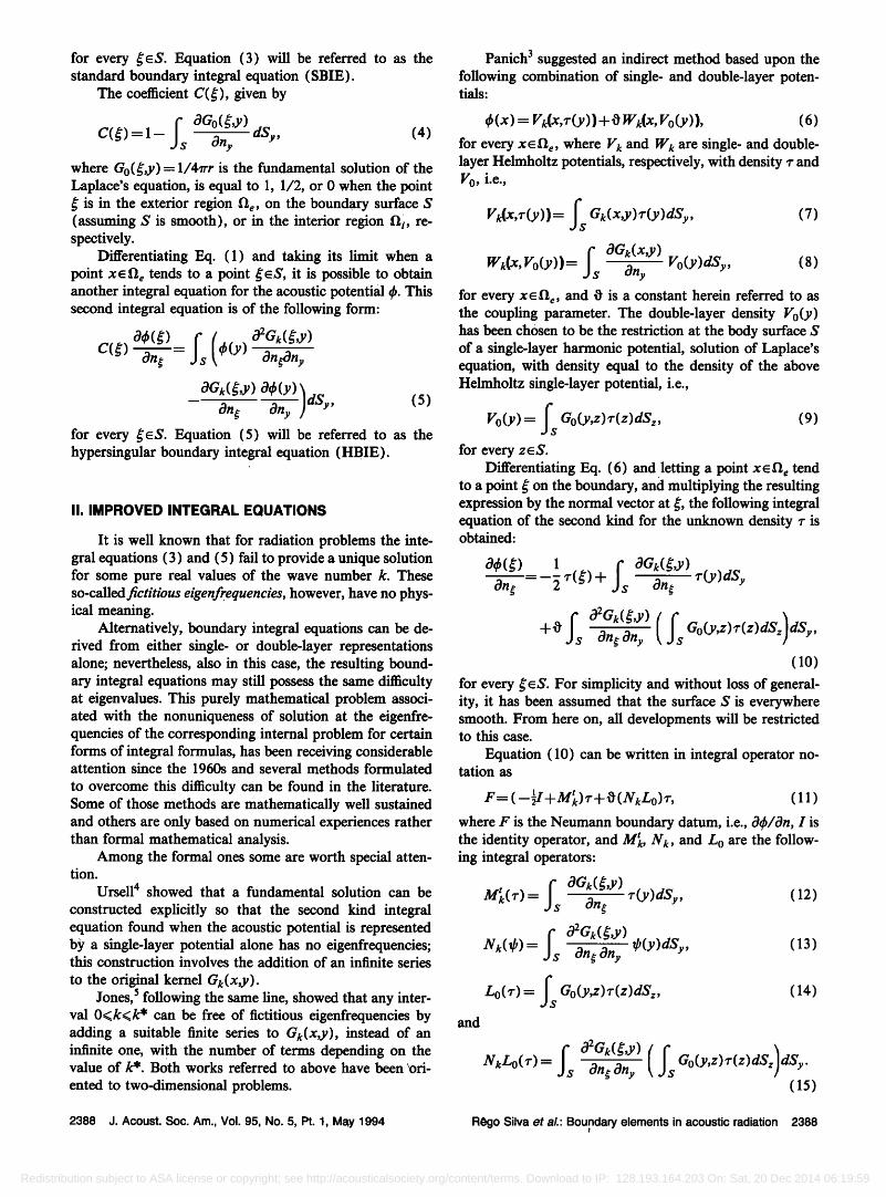
for every •S. Equation (3) will be referred to as the standard boundary integral equation (SBIE).

The coefficient C(•), given by

f s aGo(•,Y) C(•)=l- Ony dSy, (4) where Go (•,y) = 1/4frr is the fundamental solution of the Laplace's equation, is equal to 1, 1/2, or 0 when the point • is in the exterior region 11 e, on the boundary surface $ (assuming $ is smooth), or in the interior region 11 i, respectively.

Differentiating Eq. (1) and taking its limit when a point X e•e tends to a point •eS, it is possible to obtain another integral equation for the acoustic potential •. This second integral equation is of the following fo•:

C(•) 0•(•)rs( 02G•(•'Y) Ong -- • (y) On•ny

aG•(g,y) a•(y) ) -- an• any dSy, (5) for eve• •S. Equation (5) will be referred to as the hypersingular boundary integral equation (HBIE).

II. IMPROVED INTEGRAL EQUATIONS

It is well known that for radiation problems the integral equations (3) and (5) fail to provide a unique solution for some pure real values of the wave number k. These so-called fictitious eigenfrequencies, however, have no physical meaning.

Alternatively, boundary integral equations can be derived from either single- or double-layer representations alone; nevertheless, also in this case, the resulting boundary integral equations may still possess the same difficulty at eigenvalues. This purely mathematical problem associated with the nonuniqueness of solution at the eigenfrequencies of the corresponding internal problem for certain forms of integral formulas, has been receiving considerable attention since the 1960s and several methods formulated

to overcome this difficulty can be found in the literature. Some of those methods are mathematically well sustained and others are only based on numerical experiences rather than formal mathematical analysis.

Among the formal ones some are worth special attention.

Ursell 4 showed that a fundamental solution can be constructed explicitly so that the second kind integral equation found when the acoustic potential is represented b• a single-layer potential alone has no eigenfrequencies; this construction involves the addition of an infinite series

to the original kernel G•(x,y). Jones, 5 following the same line, showed that any inter-

val O<k<k* can be free of fictitious eigenfrequencies by adding a suitable finite series to G•(x,y), instead of an infinite one, with the number of terms depending on the value of k*. Both works referred to above have been \ori-

ented to two-dimensional problems.

Panich 3 suggested an indirect method based upon the following combination of single- and double-layer potentials:

ok(x) = V•(x,•'(y) )+O W•{x, Vo(y)), (6)

for every x• fie, where V• and W• are single- and double- layer Helmholtz potentials, respectively, with density •- and V0, i.e.,

V•(x,•'(y))= f s G•(x,y)•'(y)dSy, (7) f s c•Gk(x'y) Vo(y)dSy, (8) Wk(X, Vo (y ) ) = c9ny

for every X•e, and • is a constant herein referred to as the coupling parameter. The double-layer density V0(y) has been chosen to be the restriction at the body surface S of a single-layer harmonic potential, solution of Laplace's equation, with density equal to the density of the above Helmholtz single-layer potential, i.e.,

Vo(y) = f s Go(y,z)r(z)dSz, (9) for every z•S.

Differentiating Eq. (6) and letting a point x • Ile tend to a point • on the boundary, and multiplying the resulting expression by the normal vector at •, the following integral equation of the second kind for the unknown density r is obtained:

aq5(•) 1 f s aG•(•,y) c92Gl•(•,y)

+ors c9ng c9ny ( f s Gø(Y'Z)•(z)dSz) dSy' (10)

for every •S. For simplicity and without loss of general- ity, it has been assumed that the surface $ is everywhere smooth. From here on, all developments will be restricted to this case.

Equation (10) can be written in integral operator notation as

F=( • t --•I+M•)•'+O(N•Lo)•', ( 11 )

where F is the Neumann boundary datum, i.e., cgc•?cgn, I is the identity operator, and M•, N•, and L 0 are the following integral operators:

and

M•(•-) = fs c•Gk(•,y) •-(y)dSy, (12) c•ng

f $ c92Gl•(•,Y) N k ( l• ) = c9 n g C9 n y l• ( y ) dS y , (13)

Lo(•') = f s Go(y,z)•'(z)dSz, (14)

N•L0(•') = f s •G•(•,y) c9ng c9ny ( f s Gø(Y'Z)•(z)d$•) dSy' (15)

2388 J. Acoust. Soc. Am., Vol. 95, No. 5, Pt. 1, May 1994 R•go Silva et al.: Boundary elements in acoustic radiation 2388


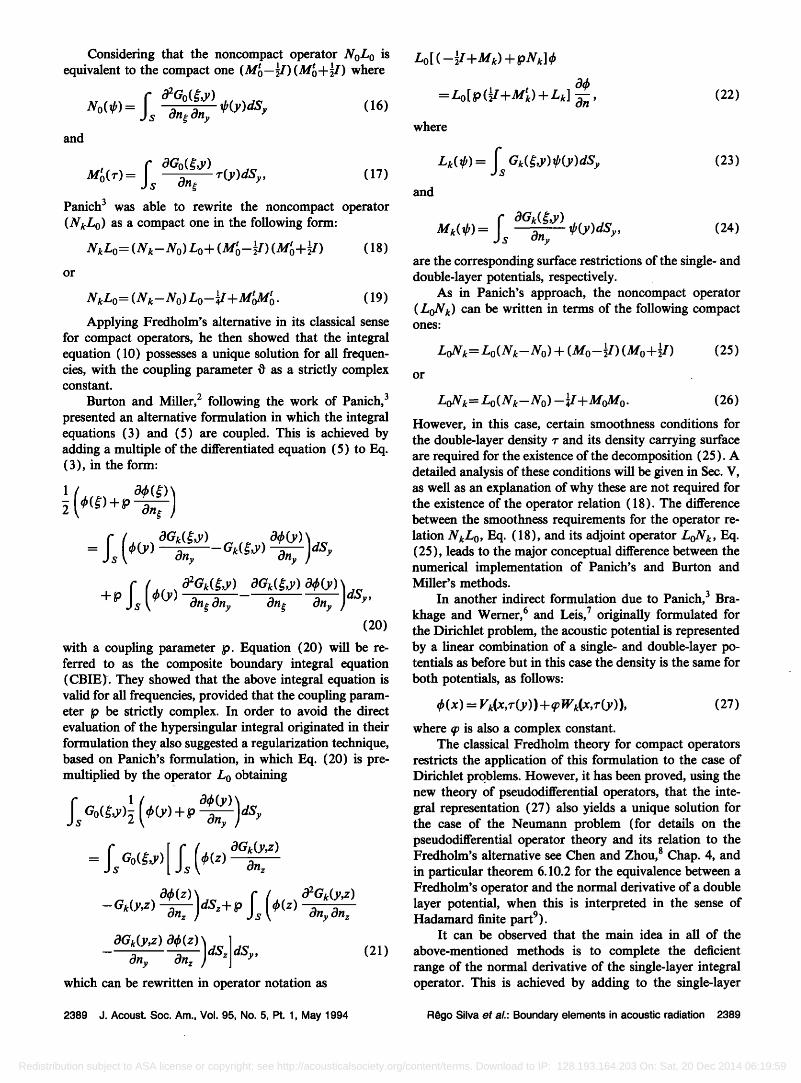
Considering that the noncompact operator NoLo is equivalent to the compact one (M•-- «I) (M• + «I) where

and

N0(•P) = angany •p(y)dSy (16)

f s aSO(g,y) M(r) = r(y)dSy, (17) Panich 3 was able to rewrite the noncompact operator (NkL o) as a compact one in the following form:

N k Lo = ( N • -- No ) Lo + ( M• -- «I ) ( M• + «I ) (18) or

N•Lo= (N•--No) Lo--¬I+ M•14r• . (19)

Applying Fredholm's alternative in its classical sense for compact operators, he then showed that the integral equation (10) possesses a unique solution for all frequencies, with the coupling parameter 0 as a strictly complex constant.

Burton and Miller, 2 following the work of Panich, 3 presented an alternative formulation in which the integral equations (3) and (5) are coupled. This is achieved by adding a multiple of the differentiated equation (5) to Eq. (3), in the form:

rs( aG•(•'Y)-G•(•'Y) &k(Y) ) rs( a2G(,y) a4(y) ) + P 4(Y) ang any -- an• any dSy,

(20)

with a coupling parameter p. Equation (20) will be referred to as the composite boundau integral equation (CBIE). They showed that the above integral equation is valid for all frequencies, provided that the coupling parameter p be strictly complex. In order to avoid the direct evaluation of the hypersingular integral originated in their fomulation they also suggested a reguladzation technique, based on Panich's fomulation, in which Eq. (20) is pre- multiplied by the operator L0 obtaining

a4(y)

1 (4(y)+p )dSy f s Gø(•'Y)• 3ny • •z

a2G•(y,z) P fs (rk(z) anyanz dSy, (21)

a(z))dSz + --G•(y,z) anz

aGk(y,z) &b(z) ) - any anz dSz which can be rewritten in operator notation as

Lo[ (--«I+Mk) +

a4 =Lo[p(«I+M•:) + L•] a•'

where

(22)

L•,(•p) = fs Gk(•,y)•b(y)dSy (23) and

f s ( g,y ) M•(tp) = any tp(y)dSy, (24) are the corresponding surface restrictions of the single- and double-layer potentials, respectively.

As in Panich's approach, the noncompact operator (LoN•) can be written in terms of the following compact ones:

LoN•= Lo(N•-No) + (Mo--«I) (Mo+«I) (25) or

LoNk= Lo( N•-No) -•I+ MoM o. (26)

However, in this case, certain smoothness conditions for the double-layer density r and its density carrying surface are required for the existence of the decomposition (25). A detailed analysis of these conditions will be given in Sec. V, as well as an explanation of why these are not required for the existence of the operator relation (18). The difference between the smoothness requirements for the operator relation N•Lo, Eq. (18), and its adjoint operator LoN•, Eq. (25), leads to the major conceptual difference between the numerical implementation of Panich's and Burton and Miller's methods.

In another indirect formulation due to Panich, 3 Bra- khage and Werner, 6 and Leis, 7 originally formulated for the Dirichlet problem, the acoustic potential is represented by a linear combination of a single- and double-layer potentials as before but in this case the density is the same for both potentials, as follows:

ok(x) = V•(x, r (y ) ) + ep Wk(x, r ( y ) ), (27)

where q• is also a complex constant. The classical Fredholm theory for compact operators

restricts the application of this formulation to the case of Dirichlet problems. However, it has been proved, using the new theory of pseudodifferential operators, that the integral representation (27) also yields a unique solution for the case of the Neumann problem (for details on the pseudodifferential operator theory and its relation to the Fredholm's alternative see Chen and Zhou, 8 Chap. 4, and in particular theorem 6.10.2 for the equivalence between a Fredholm's operator and the normal derivative of a double layer potential, when this is interpreted in the sense of Hadamard finite part9).

It can be observed that the main idea in all of the

above-mentioned methods is to complete the deficient range of the normal derivative of the single-layer integral operator. This is achieved by adding to the single-layer

2389 d. Acoust. Soc. Am., Vol. 95, No. 5, Pt. 1, May 1994 R•go Silva et aL: Boundary elements in acoustic radiation 2389


potential a regular term that perturbs the spectrum of the integral operator generated by the kernel of the normal derivative of the single-layer potential in such a way that removes the singularity of the resolvent. This complete technique is a well-established mathematical approach to define an integral representation formula that leads to a second kind integral equation with a unique solution (see Mikhlin•ø).

III. IMPROVED BOUNDARY ELEMENT METHODS

Despite the number of works on this subject it is clear that boundary element formulations still require further research to establish the most effective method for han-

dling the nonuniqueness of the radiation/scattering problem at eigenvalues of the associated internal problem, considering efficiency of the numerical scheme and accuracy of the results. A more detailed review on this matter has been

carried out by Amini et al. TM The CHIEF method, proposed by Schenck, • is consid-

ered as the most computationally efficient, and many suc- cessful results have been reported as, for instance, in Refs. 12-14. However, its lack of formalism in the selection of internal points is always a reason for concern about its consistency. •5-•7 Some major concerns, based on numerical experiences, have been reported by Piaszczyk and Klosner •8 and Reut. •9

The method of Burton and Miller 2 has then appeared as the best alternative. In its regularized form, Eq. (21), this method is considered to be computationally expensive and several techniques to deal with the hypersingular integral, to apply Eq. (20) directly, have been suggested. This method, in its hypersingular form (CBIE), has been successfully employed by Meyer et al. •5 applying piecewise constant elements, Terai 2ø who developed an analytical integration scheme applicable to flat elements, and Liu and Rizzo 2• who applied higher-order elements through a regularization of the hypersingular term. A more general approach to evaluate the hypersingular integral directly in Burton and Miller's method has recently been implemented in Ref. 22, applying the numerical technique proposed by Guiggiani et al. 23

The main disadvantage of the above method is the presence of a hypersingular integral. The key issue, however, in boundary element methods with hypersingular integrals is not their evaluation but the smoothness condition that has to be satisfied by the density function to assure the existence of the hypersingular integral (see Gunter24). It is known that the isoparametric conforming (continuous) element does not satisfy the referred condition, see for instance, Ref. 25, thus restricting this formulation to non- conforming (discontinuous) or Hermitian elements.

As Hermitian elements are difficult to implement in a three-dimensional case, and very little work using these elements can be found in the literature, the smoothness condition to guarantee the existence of the hypersingular integral has usually been satisfied through the use of discontinuous elements. Such elements, however, if applied to the whole mesh as in this case, present the drawback of

being more time consuming than the continuous ones. The use of higher order discontinuous elements tends to aggra- vate this problem.

This problem has been acknowledged by Ingber and Hickox •7 who have suggested a modified Burton-Miller algorithm in which Eq. (20) is only applied at the center node of each quadratic Lagrangian element, where the smoothness condition is satisfied, and Eq. (3) is applied at all other nodes. However, as the authors themselves point out, despite the accurate results they obtained, their algorithm lacks a formal mathematical proof and needs further study.

The formulation indicated in Eq. (27) also requires the same smoothness condition to the existence of the cor-

responding hypersingular integral. This method has been successfully employed, for instance, by Filippi 26 and Kirkup 27 not only for the Dirichlet problem but also for the Neumann problem.

Panich's method does not seem to be well known.

However, some references to his formulation have been made, e.g., by Amini et al. • confirming that the method is reliable and numerically stable, despite the absence of numerical results. Those authors have also stated that, for general application, the choice between the methods of Burton and Miller and Panich is not so clear if the smooth-

ness of the surface potential in Panich's method can be assured.

The main contribution of the present work is to present the smoothness requirements for the density function in Panich's formulation, showing that it allows for the use of continuous elements (that are at most Cø'"), which at first instance appears to violate the smoothness requirement for the existence of the corresponding hypersingular integral. This property, as pointed out before, is of fundamental importance in boundary element methods due to the computational time required for the evaluation of the coefficients of the influence matrices. The advantage of this property will be shown in the numerical examples presented, for which Panich's formulation, using continuous elements, is shown to be less time consuming than Burton and Miller's method, in which discontinuous elements are employed, even if further matrix manipulations are required.

IV. SMOOTHNESS REQUIREMENTS FOR THE DENSITY FUNCTION IN PANICH'S FORMULATION

The second kind integral equation (10) contains the term

f $ ø•2Gk(•'y) Vo(y)dSy (28) c•n g c•ny ' which is hypersingular as the integration point y approaches the source point •, hence requiring further attention in its numerical evaluation. The other integral in Eq. (10) is weakly singular since for a Lyapunov surface it is known that c9r/c9ny < Er z as r-•0, with E as a constant and it the corresponding Lyapunov exponent. Therefore, this



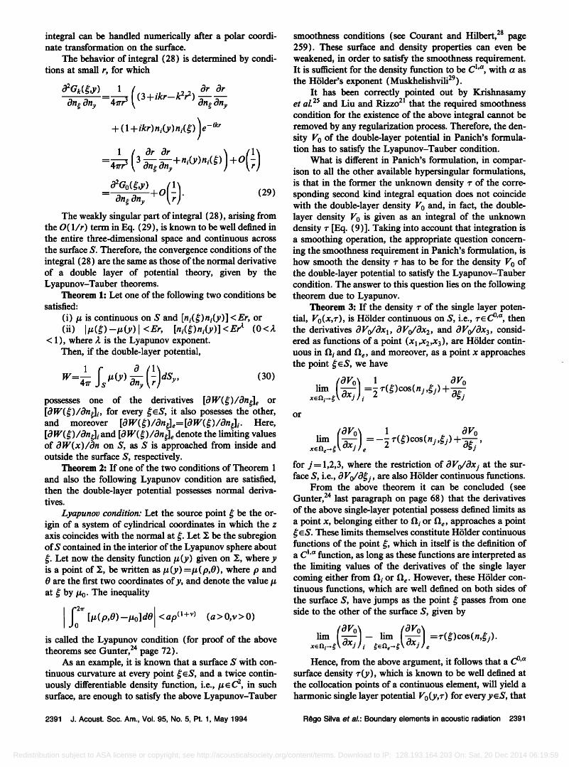
integral can be handled numerically after a polar coordinate transformation on the surface.

The behavior of integral (28) is determined by conditions at small r, for which

a2G•(•,y) 1 ( Or Or antony --4•-• ( 3+ikr-k2r•) antony

+ ( 1 +ikr)ni(y)ni(•) )e -ikr --4•---• 3 •-•n•n•+ni(y)n'(•) +0

-- On•Ony +0 . (29) The we•y singular pa• of integral (28), arising from

the O(l/r) tern in Eq. (29), is known to be well defined in the entire three-dimensional space and continuous across the surface S. Therefore, the convergence conditions of the integral (28) are the same as those of the nomal derivative of a double layer of potential theo•, given by the Lyapunov-Tauber theorems.

Theorem 1: Let one of the following two conditions be satisfied:

(i) • is continuous on S and [ni(•)ni(y)] <Er, or (ii) lu(•)-u(y)l <Er, [n•(•)ni(y)] <E•

< 1 ), where g is the Lyapunov exponent. Then, if the double-layer potential,

u(y) (30) possesses one of the derivatives [O•(•)/On•], or [O•(•)/On•] i, for eve• •& it also posesses the other, and moreover [OW(•)/On•],=[OW(•)/On•]•. Here, [OW(•)/On•]• and [OW(•)/On•], denote the limiting values of O•(x)/On on S, as S is approached from inside and outside the surface S, respectively.

Theorem 2: If one of the two conditions of Theorem 1

and also the following Lyapunov condition are satisfied, then the double-layer potential possesses nomal derivatives.

Lyapunoo condition: •t the source point • be the origin of a system of cylindrical coordinates in which the z axis coincides with the nomal at •. Let Z be the subregion of S contained in the interior of the Lyapunov sphere about •. Let now the density function •(y) given on •, where y is a point of •, be written as •(y)=•(p,O), where p and 0 are the first two coordinates of y, and denote the value • at • by •0. The inequality

• ø• [•(p,O)-•o]dO <ap (•+•) (a>0,v>0) is called the Lyapunov condition (for proof of the above theorems see Gunter, 24 page 72).

As an example, it is known that a surface S with continuous cu•ature at eve• point •S, and a twice contin- uously differentiable density function, i.e., •C 2, in such surface, are enough to satisfy the above Lyapunov-Tauber

smoothness conditions (see Courant and Hilbert, 28 page 259). These surface and density properties can even be weakened, in order to satisfy the smoothness requirement. It is sufficient for the density function to be C l'a, with a as the H61der's exponent (Muskhelishvili29).

It has been correctly pointed out by Krishnasamy et al. 25 and Liu and Rizzo 21 that the required smoothness condition for the existence of the above integral cannot be removed by any regularization process. Therefore, the density V 0 of the double-layer potential in Panich's formulation has to satisfy the Lyapunov-Tauber condition.

What is different in Panich's formulation, in comparison to all the other available hypersingular formulations, is that in the former the unknown density r of the corresponding second kind integral equation does not coincide with the double-layer density V 0 and, in fact, the double- layer density V 0 is given as an integral of the unknown density r [Eq. (9)]. Taking into account that integration is a smoothing operation, the appropriate question concerning the smoothness requirement in Panich's formulation, is how smooth the density r has to be for the density V 0 of the double-layer potential to satisfy the Lyapunov-Tauber condition. The answer to this question lies on the following theorem due to Lyapunov.

Theorem 3: If the density r of the single layer potential, Vo(x,r), is H61der continuous on S, i.e., reC ø'a, then the derivatives OV0/Ox 1, OV0/Ox 2, and OV0/Ox 3, considered as functions of a point (xl ,X2,X3), are H61der continuous in fii and fie, and moreover, as a point x approaches the point •eS, we have

or

' [ 0 I,"o'• 1 07/'0 lm '--' ----5 r(•)cos(ni,•j) q-

' [aVo\ 1 aVo zm /-:•/ = r(•)cos --, x•fle._,•k CIXj ]e --• (rtj,•j) + O•'j

for j = 1,2,3, where the restriction of OVo/OX j at the surface S, i.e., O Vo/O•j, are also H61der continuous functions.

From the above theorem it can be concluded (see Gunter, 24 last paragraph on page 68) that the derivatives of the above single-layer potential possess defined limits as a point x, belonging either to fii or fie, approaches a point •eS. These limits themselves constitute H61der continuous functions of the point •, which in itself is the definition of a C l'a function, as long as these functions are interpreted as the limiting values of the derivatives of the single layer coming either from fii or fie. However, these H61der continuous functions, which are well defined on both sides of the surface $, have jumps as the point • passes from one side to the other of the surface S, given by

. t'aVo• (OVo I •m /-•!- lim •r(•)½os(n,•i). x•fli-, • •k ClXj ] i •fle_,• • OXj / e Hence, from the above argument, it follows that a C ø'a

surface density r(y), which is known to be well defined at the collocation points of a continuous element, will yield a harmonic single layer potential Vo(y,r) for every yeS, that

2391 J. Acoust. Soc. Am., Vol. 95, No. 5, Pt. 1, May 1994 R•go Silva et al.' Boundary elements in acoustic radiation 2391


is C l'a at the collocation points, satisfying in this way the smoothness requirement for the existence of the normal derivative of the Helmholtz double-layer potential Wk(x, Vo) at the collocation points.

V. PROOF OF EXISTENCE AND UNIQUENESS OF SOLUTION IN PANICH'S FORMULATION FOR NEUMANN PROBLEMS

Panich's original work was related to the Robin problem and not to the Neumann problem as in the present case. A complete proof of uniqueness of solution for the Neumann problem will be presented here. Although this demonstration is almost the same for both problems, Pan- ich's original work 3 is only available in russian and very few references to his work can be found in the open literature. 3ø

In this section it will be shown that the second kind

integral equation (10) possesses a unique solution surface density re C ø'a, when the density carrying surface is a Ly- apunov surface and the Neumann boundary data are continuous on such surface.

Panich 3 realized that the hypersingular integral operator, obtained from taking the normal derivative of the double-layer potential in Eq. (6), can be written as a combination of certain Fredholm's integral operators. To show the relation between the above integral operators let us consider the following Laplace's single-layer potential with density r

Vo(x) = Vo(x,r) = J's Go(x,y)r(y)dSy. (31)

The above potential field is a well-defined exterior potential that satisfies the following Green's formula:

(OGo(x,y) OVo(y) )dSy= Vo(x), f s [ •9}t• Vo (y ) - Go ( x,y ) arty (32)

for every x e •e. Differentiating Eq. (32) in the direction of the normal

vector at a point •eS, and taking its limit when a point x e •e tends to the point • the following relation, for every •eS, is obtained:

OGo(•',y) OVo(y) ) On•. any dSy 10Vo(•')

=• On• ' (33) where, according to the Lyapunov-Tauber theorems, the restriction of the single-layer potential, V0, on the surface $ has to be a C l'a function, when $ is a Lyapunov surface, in order to assure the existence of the integral equation (33). As already shown in the previous section, a C ø'a surface density r is enough to guarantee a C l'a restfiction of the single-layer potential Vo(y,r) for every yeS.

Applying the jump condition at the contour surface of the normal derivative of the single-layer potential (31), coming from the exterior domain I• e, Eq. (33) can be rewritten as

f s 02Gø(•'Y) )dSy •rt•y (rs Gø(y'z)r(z)dS• 1( I fsOGo(g,y) ) =• -• r(•) + On• r(y)dSy

;sOGo(•,y)( 1 + Ong --•r(y)

f s OGø(y'z) ) + Ony r(z)dSz dSy 1

f s aCø(g'Y) ( f s aGø(y'z) ) + On• Ony r(z)dSz dSy. (34) From the above relation, it can be observed that the

following integral operator:

s O2 Go ( •,Y ) which seems to be hypersingular is, in fact, a Fredholm's integral operator, since it is known that the following product of the two compact operators:

fsOGø(g'Y)(fs øGø(y'z) ) On• Ony r(z)dS• dSy, (36) is a compact operator.

Therefore, from the above argument and the behavior of the fundamental solutions of Laplace and Helmholtz's equations for small r, the hypersingular integral operator (35) can be written in terns of the following Fredholm's operators:

fs On•Ony(fsGo(y,z)r(z) dSy - On• Ony - On• Ony )

1

+ On• On• ' which corresponds to •. (19) in operator notation.

It can be pointed out now that the above decomposition is not necessary to prove the equivalence between the hypersingular operator in Panich's fomulation and a corresponding Fredholm's operator, when the former is interpreted in the sense of Hadamard finite pa•, since this can be done with the use of the theou of pseudodifferential operators (for details see Re[ 8). However, it is presented here due to its numerical advantage.

2392 J. Acoust. Soc. Am., Vol. 95, No. 5, Pt. 1, May 1994 RSgo Silva et al.: Boundary elements in acoustic radiation 2392


Having established the compactness of the integral operators in Eq. (10), the Fredholm's alternative can be applied in order to prove the existence and uniqueness of solution of the referred integral equation. It is only necessary thus to establish that the following homogeneous equation for r ø admits only the trivial solution in the space of continuous functions:

-• rø(•) + an'••

a2G•(•m) )as• o. +of s an, an, (rs •ø(y'z)rø(z)'•sz = (38)

Equation (38) shows that the exterior acoustic potential, •o (x), given below

4ø(x) = fs •(x,y)rø(y)d$y

+o ;s aG•(•,y) any ( f s Gø(Y'Z)rø(z)dSz) ds" (39)

satisfies the homogeneous Neumann boundary condition, i.e., &bø/ang=0, for every •S. Then, by the uniqueness of the solution of the present boundary value problem, the potential •bø(x) must vanish identically in fie'

Taking into account the jump relations across the density carrying surface of the double-layer potential and normal derivative of the single-layer potential the limits, on the surface $, of the potential •b ø and its normal derivative &kø/On, coming from the domain fii interior to the surface $, are given by

and

ckø(g) =-o f s •ø(g'Y)vø(Y)d$Y' (40)

a6ø(g) •--rø(•'). (41)

Ong Applying Green's second identity for the Helmholtz's

equation to the pair •bø,•o in the interior domain fii, results in

l•e(;s•ø•'ødS):(ki2 k•r, ;•i [• 0 •nn - I•ax

+ f• IV•øl 2 dx (42) i

and

) • as =2kikr I I'•,tx, (43) i

where •b ø given by Eq. (39) and 3o, its complex conjugate, are regular solutions of the Helmholtz equations

V2•0-[- k2•0 = 0 (44) and

(45)

respectively, with k=kr+ iki and with boundary values on the surface $, coming from the interior domain, given by Eqs. (40), (41 )• and their respective complex conjugates.

Substitution of Eqs. (40) and (41 ) into Eq. (43) results in

=2krki;r• I•øl 2 dx, (46) i

The inner product between the Laplace single-layer potential, Vo(•,r ø) and the complex conjugate of the density function r ø, i.e., •o, is positive defined, i.e.,

fs•(•)(;sGo(•,y)'rø(y)dSy)>•O, (47) and assumes the value zero only if r ø =0, as will be shown below.

From the jump relation across the density carrying surface of the normal derivative of a single-layer potential the following equation is obtained:

i-- • e = •-0(•)' for every •S, where

(48)

f'ø(x) = fs Go(x,y)•(y)dSy. (49) Therefore, the inner product given in Eq. (47) can be written as

f s vø(g,rø)ds,= f s Vø( ø;'ø -•n ) •dS e

Green's first identity for the Laplace equation can now

ap ø2

be applied, resulting in

and

(51)

(52)

where the minus sign in Eq. (52) comes from the direction of the normal vector on $ in the exterior problem. There- fore, from Eqs. (50), (51 ), and (52), the following identity is obtained:

ar o 2

dx>O, (53) fs •(•) Fø(•'rø)dS•= ;n with

2393 J. Acoust. Soc. Am., Vol. 95, No. 5, Pt. 1, May 1994 R8go Silva et al.: Boundary elements in acoustic radiation 2393


Equation (53) thus will be zero only if •0 = r0 = 0, since every single la•,er with zero value at its density carrying surface has zero density, i.e., Vø(•,r ø) =0, for every • • $, imply that r ø (•) = 0.

Hence, from Eq. (46), if k is purely real (i.e., ki=0) and Im (0)=/=0, r ø has to be zero. Equation (10) then possesses a unique solution r, as long as Im (0)=/=0, for all real wave numbers k.

At this point, for the sake of clarity, it is important to distinguish between the different smoothness conditions required for the density and its carrying surface for both operators (18) and (25). As previously shown, the smoothness requirement for the existence of the operator relation (18) is that, at least, the density function re C ø'• and the surface S is a Lyapunov surface. On the other hand, these smoothness conditions are not sufficient to guarantee the existence of the operator (25) in Burton and Miller's method.

Let us now consider the following Laplace double- layer potential with density r

f s O6o(X,y) Wo(x) = Wo(x,v)= Ony v(y)d$y. (54)

The potential field (54) is a well-defined exterior potential that satisfies the following integral relation at points on the surface S, coming from its Green's formula representation:

aWo(y)) any d$y

' Wo(•) (55)

Equation (55) has its existence guaranteed only if the double-layer potential W0(y) satisfies the Lyapunov- Tauber smoothness requirements for the existence of the surface normal derivative of the double-layer potential. It is known that the above conditions are assured if, at least, the density function •'•C l'a and the surface S is a Ly- apunov surface.

In this case, the restriction of the double-layer potential Wo(y) at the surface S is given by its jump relation,

1 ;s aGo(y,z) Wo(y)=•r(y)+ anz •r(z)dSz, (56)

and its surface normal derivative is a continuous function

across its density carrying surface as long as the Lyapunov-Tauber smoothness conditions are satisfied.

Substituting Eq. (56) and the expression of the continuous normal derivative of the double layer potential (54) into Eq. (55) the following relation is obtained:

L aGo(•,y) (1 any • r(y) rs aGo(y, z) + anz • r(z)dSz)dSy _ f s Go(•,y) ( f s a2Gø(Y'Z) any Onz r(z)dSz)dSy 1(1 ;s aGo(•',y) ) =5 5 r(g) + any r(y)dSy

or, equivalently,

f s Go(,,y) ( f s a2Gø(Y'Z) r(z)dSz)dSy 1

=-•r(•)

(57)

+ fs aGo(•,y)( aGo(y,z) r(z)dSz)dSy (58) 0% f s Onz ' which can be written in operator notation as

•dv0= !M0-«•) (M0+«•) = --•+Mom0. (59) Hence, in order to guarantee the existence of Eq. (59),

and consequently the existence of Eq. (26), the density r has to be a C •'a function and the surface S has to be a Lyapunov surface. It is interesting to point out that these smoothness conditions are the required conditions for the formal proof of existence and uniqueness of solution for Burton and Miller's formulation given by Lin in Ref. 31.

VI. NUMERICAL IMPLEMENTATION

Equation ( 11 ) will be numerically implemented in the following form:

F= ( --«I+M•)r+O((N•,--No) Lo--•I+M•I'I•)r, (60)

in which the decomposition (19) has been taken into account. The integrals (12) to (17) are to be evaluated over each element after the boundary discretization.

In this work the boundary is discretized employing quadratic isoparametric continuous elements, triangular and quadrilateral. Following the general procedure in boundary element methods, the geometry is approximated by shape functions q•,

Mi

Xi= Z kll(nl,n2)x7, (61) m=l

where M/is the number of geometric nodes in each element F l .

The density in each integral needed in Eq. (60) is approximated by interpolation functions ß as follows:

f r aG•(•,Y) M•= , • (I) (nl ,n2)I]lar,, (62)

fr (a•(;•(•'y) a•ø(•'Y)) N•,-- No = • an g any -- an g any X (I)(nl ,n2)IJIdr•, (63)

2394 d. Acoust. Soc. Am., Vol. 95, No. 5, Pt. 1, May 1994 R•go Silva et aL: Boundary elements in acoustic radiation 2394


L0-- ;r Go(y,z)•(•l•,•72) IJIdr•, (6•) l

It is impo•ant to point out that the above integrals do not require any special considerations to their numerical evaluation and a standard Gauss integration scheme can be applied. The singular integration of the ke•els of order O(l/r) are directly handled after applying a polar coordinate transfo•ation. For the case of regular integration the transfo•ation of coordinates proposed by Telles 32 has also been applied for quasisingular integrals with a selective choice of number of integration points.

The potential on the boundary is then evaluated by

•(g) = [Lk+O(• I+MkLo) ]•, (66)

with the operators Lk and M k given by

Lk-- fr G•:(Y'Z)•P(•7•'•72) IJIdF•, l

(67)

fr •G•(g'y) •(•,•72)IJIdr•, (68) M• = Ony which, for computational efficiency, are evaluated together with (62) to (65).

VII. CHOICE OF THE COUPLING PARAMETER O

Another relevant issue in this type of formulation is the choice of the coupling parameter. Several works, based on numerical experience, have been reported concerning the optimal choice for the formulations represented by (20), (21), and (27) showing that it can significantly af- fect the accuracy of the results. 15'27'33-35 Amini 36 has suggested some optimal values for Burton-Miller's method represented by (20) and (21), based on a more formal mathematical analysis.

For Panich's formulation, a systematic approach for the choice of the coupling parameter 0 has not yet been reported in the literature. However, due to its similarity to the integral representation (21) the value 0--4 suggested in Ref. 36 for that expression, has been used. According to the numerical results obtained here, the value 0-i gives more accurate results than O-i/k, another common choice.

Viii. NUMERICAL RESULTS

In order to verify the performance of the proposed numerical technique three examples have been analyzed. These have been chosen because of the availability of analytical or numerical solutions. In the following examples the present formulation will be referred to as the improved boundary integral equation (IBIE).

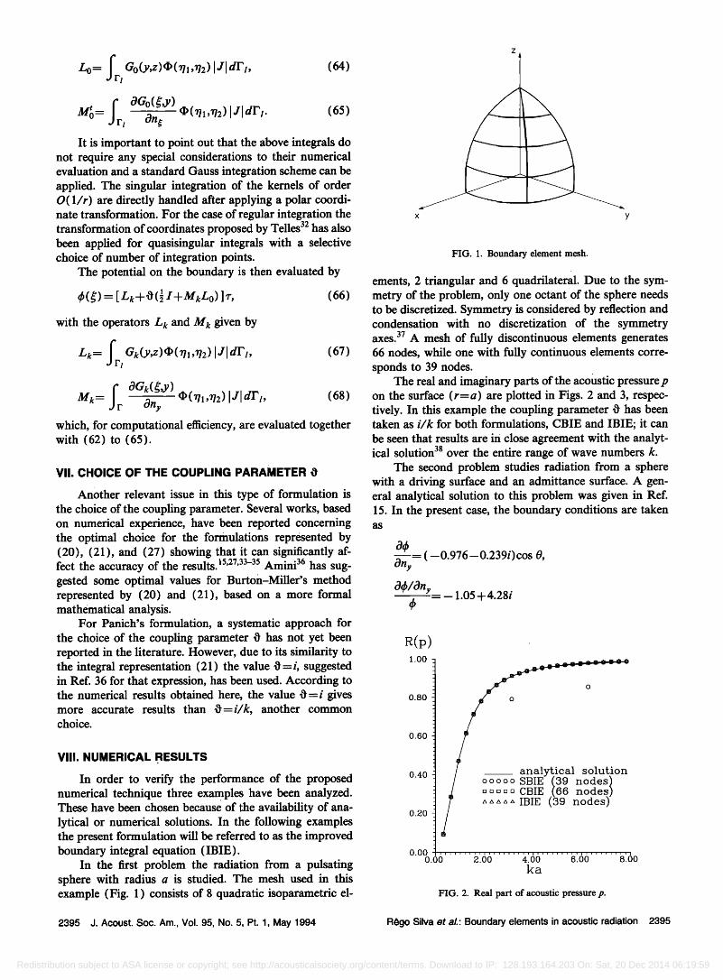
In the first problem the radiation from a pulsating sphere with radius a is studied. The mesh used in this example (Fig. 1 ) consists of 8 quadratic isoparametric el-

x y

FIG. 1. Boundary element mesh.

ements, 2 triangular and 6 quadrilateral. Due to the symmetry of the problem, only one octant of the sphere needs to be discretized. Symmetry is considered by reflection and condensation with no discretization of the symmetry axes. 37 A mesh of fully discontinuous elements generates 66 nodes, while one with fully continuous elements corresponds to 39 nodes.

The real and imaginary parts of the acoustic pressure œ on the surface (r--a) are plotted in Figs. 2 and 3, respectively. In this example the coupling parameter 0 has been taken as i/k for both formulations, CBIE and IBIE; it can be seen that results are in close agreement with the analytical solution 38 over the entire range of wave numbers k.

The second problem studies radiation from a sphere with a driving surface and an admittance surface. A general analytical solution to this problem was given in Ref. 15. In the present case, the boundary conditions are taken as

a½ -- ( --0.976--0.239i)cos 0,

any

a/an, -- 1.05-1-4.28i

1.00 -

0.80

0.60

0.40

0.20

lution

/ ooooo SBIE- (39 nodes) .• [][][][][] CBIE .(66 nodes)

•• IBIE (39 nodes) 0.00 ..........................

o.oo • 66 •,:66 /3'.66 •'.6o ka

FIG. 2. Real part of acoustic pressure œ.

2395 J. Acoust. Soc. Am., Vol. 95, No. 5, Pt. 1, May 1994 R8go Silva et al.: Boundary elements in acoustic radiation 2395


I(p) 0.60

0.50

0.40

0.30

0.20

analytical solution

ooooo SBIE (3•½ nodes) [] [] [] [] [] CBIE nodes.) • • • • • IBIE nodes)

o

0.10 o.oo •.6o •.66 ...... b'.6o a.6o

ka

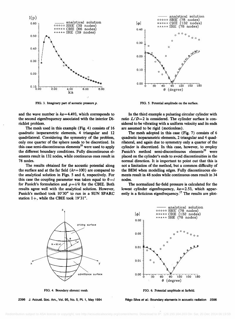
FIG. 3. Imaginary part of acoustic pressure p.

I½ 0.40 -

0.30

0.20

0.10

0.00

analytical solution ooooo SBIE (78 nodes). [][][][][] CBIE (132 node. s) •• IBIE (78 nodes)

o o o o

o o o

, , i , , øl ,V, i , , i , , i 0 30 60 90 120 150 180

0 (degree)

FIG. 5. Potential amplitude on the surface.

and the wave number is ka=4.493, which corresponds to the second eigenfrequency associated with the interior Di- richlet problem.

The mesh used in this example (Fig. 4) consists of 16 quadratic isoparametric elements, 4 triangular and 12 quadrilateral. Considering the symmetry of the problem, only one quarter of the sphere needs to be discretized. In this case semi-discontinuous elements 39 were used to apply the different boundary conditions. Fully discontinuous elements result in 132 nodes, while continuous ones result in 78 nodes.

The results obtained for the acoustic potential along the surface and at the far field (kr= 100) are compared to the analytical solution in Figs. 5 and 6, respectively. For this case the coupling parameter was taken equal to 0 =i for Panich's formulation and p=i/k for the CBIE. Both results agree well with the analytical solution. However, Panich's method took 10'30" to run in a SUN SPARC

station 1 +, while the CBIE took 19'31".

driving surface

y

admittance surface


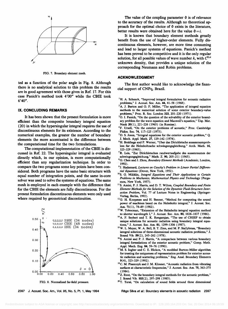
In the third example a pulsating circular cylinder with ratio L/D=2 is considered. The cylinder surface is considered to be vibrating with a uniform velocity and its ends are assumed to be rigid (motionless).

The mesh adopted in this case (Fig. 7) consists of 6 quadratic isoparametric elements, 2 triangular and 4 quadrilateral, and again due to symmetry only a quarter of the cylinder is discretized. In this case, however, to employ Panich's method semi-discontinuous elements 39 were placed on the cylinder's ends to avoid discontinuities in the normal direction. It is important to point out that this is not a limitation of the method, but a common difficulty of the BEM when modelling edges. Fully discontinuous elements result in 48 nodes while continuous ones result in 34

nodes.

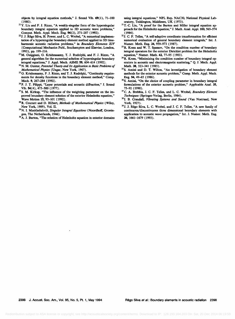
The normalized far-field pressure is calculated for the lowest cylinder eigenfrequency, ka=2.53, which appar- ently is a fictitious eigenfrequency. •7 The results are plot-

analytical solution

ooooo ( I½1 ooooo CBIE 2 no • • • • • IBIE nodes)

0.02

o o o

0.02 o o o o o o

o

0.01 • . o • • •

0.01

0.00 , , , , , , .... , ...... 0 30 60 90 120 150 180

0 (degree)

FIG. 6. Potential amplitude at farfield.



z


ted as a function of the polar angle in Fig. 8. Although there is no analytical solution to this problem the results are in good agreement with those given in Ref. 17. For this case Panich's method took 4'00" while the CBIE took

IX. CONCLUDING REMARKS

It has been shown that the present formulation is more efficient than the composite boundary integral equation (20) in which the hypersingular integral requires the use of discontinuous elements for its existence. According to the numerical examples, the greater the number of boundary elements the more accentuated is the difference between

the computational time for the two formulations. The computational implementation of the CBIE is dis-

cussed in Ref. 22. The hypersingular integral is evaluated directly which, in our opinion, is more computationally efficient than any regularization technique. In order to compare the two programs some key points have been considered. Both programs have the same basic structure with equal number of integration points, and the same in-core solver was used to solve the systems of equations. The same mesh is employed in each example with the difference that for the CBIE the elements are fully discontinuous. For the present formulation discontinuous elements were only used where required by geometrical discontinuities.

0.50 II ß

• [] [] [] [] [] CBIE nodess) o.4o - • • • • • IBIE nodes)

0.30

0.E0

0.10

0.00 0.00 0.;80 0.4-0 0.60 0.80 1.00

FIG. 8. Normalized far-field pressure.

The value of the coupling parameter 0 is of relevance to the accuracy of the results. Although no theoretical approach for the optimal choice of 0 exists in the literature, better results were obtained here for the value 0--i.

It is known that boundary element methods greatly benefit from the use of higher-order elements. Fully discontinuous elements, however, are more time consuming and lead to larger systems of equations. Panich's method has been proved to be competitive and it is the only regular solution, for all possible values of wave number k, with C ø'a unknown density, that provides a un!que solution of the corresponding Neumann and Robin problems.

ACKNOWLEDGMENT

The first author would like to acknowledge the finan- cial support of CNPq, Brazil.

•H. A. Schenck, "Improved integral formulation for acoustic radiation problems," J. A½oust. So½. Am. 44, 41-58 (1968).

2A. J. Burton and G. F. Miller, "The application of integral equation methods to the numerical solution of some exterior boundary-value problems," Pro½. R. So½. London 323, 201-220 (1971).

30. I. Panich, "On the question of the solvability of the exterior boundary problem for the wave equation and Maxwell's equation," Usp. Mat. Nauk 20(1 ), 221-226 (1965) (in Russian).

4F. Ursell, "On the exterior problems of acoustic," Proc. Cambridge Philos. So½. 74, 117-125 (1973).

5D. S. Jones, "Integral equations for the exterior acoustic problem," Q. J. Mech. Appl. Math. 27, 129-142 (1974).

6H. Brakhage and P. Werner, "Uber das Dirichletsche aussenraumprob- lem fur die Helmholtzsche schwingungsgleichung," Arch. Math. 16, 325-329 (1965).

7 R. Leis, "Zur Dirichletschen randwertaufgabe des aussenraumes der schwingungsgleichung," Math. Z. 90, 205-211 (1965).

8 G. Chen and J. Zhou, Boundary Element Methods (Academic, London, 1992).

9 j. Hadamard, Lectures on Cauchy's Problem in Linear Partial Differen- tial Equations (Dover, New York, 1952).

løs. G. Mikhlin, Integral Equations and Their Applications to Certain Problems in Mechanics, Mathematical Physics and Technology (Perga- mon, New York, 1957).

l l S. Amini, P. J. Harris, and D. T. Wilton, Coupled Boundary and Finite Element Methods for the Solution of the Dynamic Fluid-Structure Inter- action Problem, Vol. 77 of Lecture Notes in Engineering (Springer- Verlag, Berlin, 1992).

12G. H. Koopman and H. Benner, "Method for computing the sound power of machines based on the Helmholtz integral," J. Acoust. Soc. Am. 71(1), 78-89 (1982).

•3W. Tobocman, "Extension of the Helmholtz integral equation method to shorter wavelength I," J. Acoust. Soc. Am. 80, 1828-1837 (1986).

14A. F. Seybert and T. K. Rengarajan, "The use of CHIEF to obtain unique solutions for acoustic radiation using boundary integral equations," J. Acoust. Soc. Am. 81, 1299-1306 (1987).

15W. L. Meyer, W. A. Bell, B. T. Zinn, and M.P. Stallybrass, "Boundary integral solutions of three-dimensional acoustic radiation problems," J. Sound ¾ib. 59(2), 245-262 (1978).

•6S. Amini and P. J. Harris, "A comparison between various boundary integral formulations of the exterior acoustic problem," Comp. Meth. Appl. Mech. Eng. 84, 59-76 (1990).

•7 M. S. Ingber and C. E. Hickox, "A modified Burton-Miller algorithm for treating the uniqueness of representation problem for exterior acoustic radiation and scattering problems," Eng. Anal. Boundary Elements 9(4), 323-329 (1992).

18 C. M. Piaszczyk and J. M. Klosner, "Acoustic radiation from vibrating surfaces at characteristic frequencies," J. Acoust. Soc. Am. 75, 363-375 (1984).

19 Z. Reut, "On the boundary integral methods for the acoustic problem," J. Sound ¾ib. 103(2), 297-298 (1985).

2øT. Terai, "On calculation of sound fields around three dimensional



objects by integral equation methods," J. Sound Vib. 69(1), 71-100 (1980).

2• y. Liu and F. J. Rizzo, "A weakly-singular form of the hypersingular boundary integral equation applied to 3D acoustic wave problems," Comput. Meth. Appl. Mech. Eng. 96(2), 271-287 (1992).

22 j. j. Rf•go Silva, H. Power, and L. C. Wrobel, "A numerical implementation of a hypersingular boundary element method applied to 3D time- harmonic acoustic radiation problems," in Boundary Elements (Computational Mechanics Publ., Southampton and Elsevier, London, 1992), pp. 199-216.

23M. Guiggiani, G. Krishnasamy, T. J. Rudolphi, and F. J. Rizzo, "A general algorithm for the numerical solution of hypersingular boundary integral equations," J. Appl. Mech. ASME 59, 604-614 (1992).

24 N.M. Gunter, Potential Theory and Its Application to Basic Problems of Mathematical Physics (Ungar, New York, 1967).

25 G. Krishnasamy, F. J. Rizzo, and T. J. Rudolphi, "Continuity requirements for density functions in the boundary element method," Comp. Mech. 9, 267-284 (1992).

26p. j. T. Filippi, "Layer potentials and acoustic diffraction," J. Sound Vib. $4(4), 473-500 (1977).

27 S. M. Kirkup, '•he influence of the weighting parameter on the improved boundary element solution of the exterior Helmholtz equation," Wave Motion 15, 93-101 (1992).

28 R. Courant and D. Hilbert, Methods of Mathematical Physics (Wiley, New York, 1989), Vol. II.

29N. I. Muskhelishvili, Singular Integral Equations (Noordhoff, Gronin- gen, The Netherlands, 1946).

30 A. J. Burton, "The solution of Helmholtz equation in exterior domains

using integral equations," NPL Rep. NAC30, National Physical Lab- oratory, Teddington, Middlesex, UK (1973).

3• T.-C. Lin, "A proof for the Burton and Miller integral equation approach for the Helmholtz equation," J. Math. Anal. Appl. 103, 565-574 (1984).

32 j. C. F. Telles, "A self-adaptive coordinate transformation for efficient numerical evaluation of general boundary element integrals," Int. J. Numer. Meth. Eng. 24, 959-973 (1987).

33R. Kress and W. T. Spassov, "On the condition number of boundary integral operators for the exterior Dirichlet problem for the Helmholtz equation," Numer. Math. 42, 77-95 (1983).

34 R. Kress, "Minimizing the condition number of boundary integral operators in acoustic and electromagnetic scattering," Q. J. Mech. Appl. Math. 38, 323-341 (1985).

35S. Amini and D. T. Wilton, "An investigation of boundary element methods for the exterior acoustic problem," Comp. Meth. Appl. Mech. Eng. 54, 49-65 (1986).

36S. Amini, "On the choice of coupling parameter in boundary integral formulations of the exterior acoustic problem," Applicable Anal. 35, 75-92 (1990).

37 C. A. Brebbia, J. C. F. Telles, and L. C. Wrobel, Boundary Element Techniques (Springer-Verlag, Berlin, 1984).

35I. B. Crandall, Vibrating Systems and Sound (Van Nostrand, New York, 1927).

39j. j. Rf•go Silva, L. C. Wrobel, and J. C. F. Telles, "A new family of continuous/discontinuous three dimensional boundary elements with application to acoustic wave propagation," Int. J. Numer. Meth. Eng. 36, 1661-1679 (1993).

2398 J. Acoust. Soc. Am., Vol. 95, No. 5, Pt. 1, May 1994 R{)go Silva et aL: Boundary elements in acoustic radiation 2398


Documents

The use of C0,α boundary elements in an improved numerical formulation for three-dimensional acoustic radiation problems