1

The Use of Rosseland- and Planck-Averaged Opacities in

Multigroup Radiation Diffusion

Pranav Devarakonda

Brighton High School, 1150 Winton Road, Rochester, NY

LLE Advisor: Dr. Reuben Epstein

Laboratory for Laser Energetics, University of Rochester, Rochester, NY

August 2015

2

Abstract

Opacity quantifies how strongly radiation is absorbed while passing through a material.

Hydrocodes at LLE and elsewhere use opacity values averaged over large intervals of the

radiation spectrum to calculate radiation energy diffusion transport within plasmas. This work

compares two-opacity modeling, where Planck averages are used for emission and absorption

and Rosseland averages are used for transport, with the treatment in LLE hydrocodes where a

single opacity (typically the Planck average) is used. Planck and Rosseland interval-averaged

opacities for Si were obtained by running the Prism detailed atomic model PROPACEOS. An

analytic solution was then derived for the radiation diffusion equation in a slab-source problem

in which separate opacities were used for absorption and transport. Results for the emitted

spectral flux were compared for the preferred two-opacity case and for the case where a single,

Planck opacity was used. Even when the Planck and Rosseland averages differed, the differences

in flux were minimal except for spectral intervals where the optical depth was approximately 1.

3

1. Introduction

At the University of Rochester’s Laboratory for Laser Energetics (LLE) and the National

Ignition Facility (NIF),1 research is done on laser fusion where laser energy is used to compress a

capsule, bringing its fuel contents to thermonuclear fusion conditions.2 There are two main types

of laser fusion: direct drive and indirect drive. The Laboratory for Laser Energetics deals mainly

with direct drive. In direct drive, a capsule’s outer surface is irradiated directly by the laser

beams, as opposed to indirect drive, where the inner surface of a small container enclosing the

capsule is irradiated by laser beams entering the enclosure through laser entrance holes,

generating thermal radiation that implodes the capsule.

The target is a spherical cryogenic capsule approximately 10 μm thick with a diameter of

~860 μm, coated on the inside with approximately 65 μm of deuterium-tritium (DT) ice, and

filled with three atmospheres of DT. 3 The laser is the 60 beam OMEGA laser system, 4 one of

the most powerful in the world. During direct-drive inertial confinement fusion, the laser pulses

partially ablate the surface of the capsule, causing it to rocket off, and compress the capsule,

along with its DT contents, to conditions of high temperature and density. At a sufficiently high

temperature, the deuterium and tritium undergo fusion reactions to form helium, a neutron, and

large amounts of energy. A large amount of thermal energy is needed to give the colliding nuclei

the large thermal velocities needed to overcome their large electrostatic repulsion.

The amount of energy produced by the inertial confinement fusion process can be

inferred from the measured neutron yield. LLE uses simulation programs, such as the one-

dimensional hydrodynamics code LILAC,5 to predict the outcome of these experiments. A

significant factor affecting the outcome of inertial confinement fusion experiments is the x-ray

opacity of the imploding capsule. Opacity is a measure of impenetrability of electromagnetic or

4

other kinds of radiation.6,7 The current hydrodynamic codes use one type of averaged spectral-

interval opacity, the Planck-averaged opacity. This work explores whether Rosseland-averaged

opacity should also be used in the computational codes.8

2. Equations of Radiative Transfer

The hydrodynamic simulation code LILAC5 is one of several used at the Laboratory for

Laser Energetics that includes a radiation diffusion transport model. The codes are all similar, in

that they all compute several important quantities such as radiation energy density Uν, the

spectral flux Fν, scale length λν, and optical depth τν. These quantities are functions of the

spectral frequency ν of the radiation and the local temperature T and material density. LILAC is

unique in that it models plasma flow with spherical, cylindrical, or planar symmetry and spatial

variation in only one dimension. Consequently, in this work, where we consider how radiation

transport might be done differently, 1D radiation transport, as LILAC does it, is a logical point of

reference. Other simulation codes at LLE use radiative opacity in similar ways, so the lessons

learned in this work will have relevance to them as well.

Opacity is defined as the quantitative measure of how strongly radiation is absorbed

while passing through a material. Optical depth is a dimensionless quantity defined as the

integral of opacity with respect to distance. If the optical depth is much greater than 1, the source

is considered to be optically thick, and, conversely, if the optical depth of the source is much less

than 1, the source is considered to be optically thin. The following equation expresses the optical

depth at the spectral frequency ν:

𝜏𝜈 = ∫𝜅𝜈𝑑𝑑, (2.1)

5

where κν is the opacity at frequency ν and s is the distance along a path through the source. The

value of the optical depth depends on the choice of this path.6,7 The quantities of spectral flux Fν

and radiation energy density Uν are closely related in the time-independent diffusion

approximation by the following equations,

𝐹𝜈 = − 𝑐3𝜅𝜈

𝑑𝑈𝜈𝑑𝑑

(2.2a)

𝑑𝐹𝜈𝑑𝑑

= 𝜀𝜈 − 𝑐𝜅𝜈𝑈𝜈, (2.2b)

where c is the speed of light and εν is emissivity (emitted spectral power per unit volume) at

frequency ν.8 Equations (2.2) are written for 1D plane-parallel geometry where the path length

parameter s is the spatial coordinate in the one spatial dimension. The diffusion approximation

arises from the assumption that radiation is defined as a locally isotropic spectral energy density

of photons plus a small flux in a single direction along the gradient of Uν. Equation (2.2a) gives

the magnitude of this radiation flux in terms of this gradient of the radiation energy density, and

Eq. (2.2b) equates the divergence of this radiation flux to the total radiation emission-minus-

absorption at a given point. Equations (2.2a) and (2.2b) can be solved simultaneously for Uν and

Fν . These two equations can be combined into one by eliminating Fν, leaving the more familiar

diffusion equation, a 2nd-order differential equation for Uν,8

0 = − 𝑑𝑑𝑑� 𝑐3𝜅𝜈

𝑑𝑈𝜈𝑑𝑑�+𝜀𝜈 − 𝑐𝜅𝜈𝑈𝜈. (2.3)

When calculating radiation transport numerically over the whole spectrum, the spectrum

is divided into a finite number of frequency intervals or “groups,” where the spectral frequency

group index k refers to the frequency interval from νk to νk+1. This frequency grouping should

6

be as fine as necessary to resolve the spectrum, but there should also be as few groups as

possible to minimize the time and other computational resources required to complete the

calculation. This “multigroup” formulation is constructed by replacing the frequency-dependent

flux, energy density, emissivity, and opacity quantities in Eqs. 2.2a, 2.2b, and 2.3 with group-

averaged quantities:

𝐹𝑘 = − 𝑐3𝜅𝑅,𝑘

𝑑𝑈𝑘𝑑𝑑

(2.4a)

𝑑𝐹𝑘𝑑𝑑

= 𝜀𝑘 − 𝑐𝜅𝑃,𝑘𝑈𝑘. (2.4b)

The group-averaged emissivity is obtained using

𝜀𝑘 =∫ 𝜀𝜐𝑑𝑑𝜐𝑘+1𝜐𝑘𝑑𝑘+1−𝑑𝑘

, (2.5)

and the flux Fk and energy density Uk averages are obtained by the same method. 6,8

For Eq. (2.4a) to be consistent with Eq. (2.2a), the group-average opacity κR,k must be

1

𝜅𝑅,𝑘=

∫ 1𝜅𝜈

𝑑𝑈𝜈𝑑𝑑 𝑑𝜈

𝜈𝑘+1𝜈𝑘

∫ 𝑑𝑈𝜈𝑑𝑑 𝑑𝜈

𝜈𝑘+1𝜈𝑘

, (2.6a)

and for Eq. (2.4b) to be consistent with Eq. (2.2b), the group-average opacity κP,k must be

𝜅𝑃,𝑘 =∫ 𝑈𝜈𝜅𝜈𝑑𝜈𝜈𝑘+1𝜈𝑘∫ 𝑈𝜈𝑑𝜈𝜈𝑘+1𝜈𝑘

. (2.6b)

Equations (2.6) show that calculating the multigroup average opacity quantities requires that the

radiation energy density Uν frequency dependence be known in sub-group detail, i.e., in finer

7

spectral detail than the multigroup spectral resolution can provide. We can proceed with the

multigroup method by approximating the weighting functions in Eqs. (2.6) with the radiation

energy density known to exist under conditions of local thermodynamic equilibrium,8

𝑈𝜈 = 4𝜋𝑐𝐵𝜈(𝑇), (2.7a)

where Bν(T) is the Planck function

𝐵𝜈(𝑇) = 2ℎ𝜈3

𝑐21

𝑒ℎ𝜈/𝑘𝐵𝑇−1, (2.8)

and where h is the Planck constant and kB is the Boltzmann constant. This approximation was

originally devised for the deep interior of stars, where it is an excellent approximation.7 Other

than this precedent, we have no well-developed justification for using this approximation in laser

fusion. We can also write

𝑑𝑈𝜈𝑑𝑑

= 4𝜋𝑐𝑑𝐵𝜈(𝑇)𝑑𝑇

𝑑𝑇𝑑𝑑

. (2.7b)

The two kinds of opacity average which we will explore are the Planck-averaged opacity,

obtained from Eqs. (2.6b) and (2.7a), computed as an arithmetic mean weighted by the Planck

function,

𝜅𝑃,𝑘 ≡∫ 𝐵𝜈𝜅𝜈𝑑𝜈𝜈𝑘+1𝜈𝑘∫ 𝐵𝜈𝑑𝜈𝜈𝑘+1𝜈𝑘

, (2.9a)

and the Rosseland-averaged opacity, obtained from Eqs. (2.6a) and (2.7b), computed as a

harmonic mean weighted by the derivative of the Planck function with respect to temperature,8

8

1𝜅𝑅,𝑘

≡∫ 1

𝜅𝜈𝑑𝐵𝜈𝑑𝑇 𝑑𝜈

𝜈𝑘+1𝜈𝑘

∫ 𝑑𝐵𝜈𝑑𝑇 𝑑𝜈

𝜈𝑘+1𝜈𝑘

. (2.9b)

The temperature gradient dT/ds in Eq. (2.7b) cancels out of the quotient in Eq. (2.6a).

Just as the arithmetic mean of a set of data is always greater than or equal to the harmonic

mean, the Planck-averaged opacity is generally greater than or equal to the Rosseland-averaged

opacity, assuming that the weighting functions do not greatly impact the averages. As the

number of groups increases and as the individual groups narrow to the point where the spectral

features of the opacity begin to be resolved by the frequency groups, the differences between the

Planck and Rosseland averages become less important, and the choice of the weighting functions

becomes less critical. Unfortunately, computational limits on spectral resolution may not allow a

number of frequency groups large enough to achieve this.

The tabulated group-averaged emissivity εk is generally obtained as part of the same

atomic-physics calculation used to obtain the group-averaged opacity or opacities. Under

conditions of local thermodynamic equilibrium, which is assumed here, the emissivity is related

to the opacity by the Kirchoff relationship9

𝜀𝜈 = 4𝜋𝜅𝜈𝐵𝜈(𝑇). (2.10)

Equation (2.7a) is, in part, a consequence of Eq. (2.10). Using Eq. (2.10) in Eq. (2.5) and

applying Eq. (2.9a) gives the expression

𝜀𝑘 =4𝜋𝜅𝑃,𝑘 ∫ 𝐵𝜈(𝑇)𝑑𝜈𝜈𝑘+1

𝜈𝑘𝜈𝑘+1−𝜈𝑘

, (2.11)

9

which relates the group-averaged emissivity εk to the Planck-averaged opacity κP,k.

Consequently, εk will not be changed by varying κR,k, as long as κP,k is left constant.

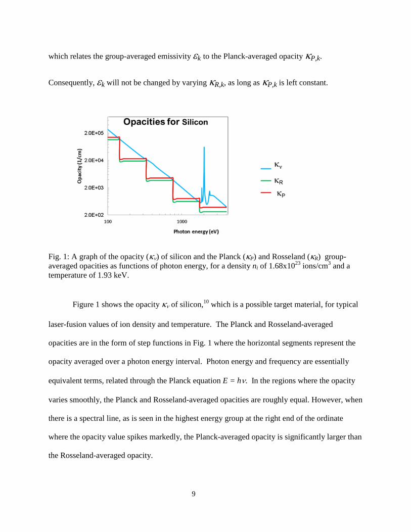
Fig. 1: A graph of the opacity (κν) of silicon and the Planck (κP) and Rosseland (κR) group-averaged opacities as functions of photon energy, for a density ni of 1.68x1023 ions/cm3 and a temperature of 1.93 keV.

Figure 1 shows the opacity κν of silicon,10 which is a possible target material, for typical

laser-fusion values of ion density and temperature. The Planck and Rosseland-averaged

opacities are in the form of step functions in Fig. 1 where the horizontal segments represent the

opacity averaged over a photon energy interval. Photon energy and frequency are essentially

equivalent terms, related through the Planck equation E = hν. In the regions where the opacity

varies smoothly, the Planck and Rosseland-averaged opacities are roughly equal. However, when

there is a spectral line, as is seen in the highest energy group at the right end of the ordinate

where the opacity value spikes markedly, the Planck-averaged opacity is significantly larger than

the Rosseland-averaged opacity.

10

In this work, two-opacity modeling, where the Planck average is used for emission

(through Eq. (2.11)) and absorption in Eq. (2.4b) and the Rosseland average is used for transport

in Eq. (2.4a), is compared with the single-opacity treatment in LLE hydrocodes where a single

opacity (typically the Planck average) is used for all purposes.

3. The Slab Source Problem

The slab source problem is a common illustrative example in radiation transport

literature. The slab source problem assumes a uniform slab of thickness L under conditions of

uniform composition, temperature, and density. This provides a slab with spatially uniform

opacity and emissivity where the general solution to Eqs. (2.4a) and (2.4b) is

𝑈𝑘(𝑥) = 𝐶0 − 𝐶1𝑒�3𝜅𝑃,𝑘𝜅𝑅,𝑘𝑥 − 𝐶2𝑒−�3𝜅𝑃,𝑘𝜅𝑅,𝑘𝑥, (3.1a)

and, by Eq. (2.4a),

𝐹𝑘(𝑥) = 𝑐�𝜅𝑃,𝑘

3𝜅𝑅,𝑘�𝐶1𝑒�3𝜅𝑃,𝑘𝜅𝑅,𝑘𝑥 − 𝐶2𝑒−�3𝜅𝑃,𝑘𝜅𝑅,𝑘𝑥�, (3.1b)

where x is the spatial coordinate in the direction normal to the slab. The constant C0 is

determined by substitution into Eqs (2.4a) and (2.4b),

𝐶0 = 𝜀𝑘𝑐𝜅𝑃,𝑘

, (3.1c)

and the constants C1 and C2 are set by a zero-flux condition at the center plane of the slab and by

a surface flux boundary condition. At the center plane of the slab, x=0, there is no net flux in

either direction because the positive and negative x directions are equivalent, so C1 = C2 from

Eq. (3.1b). At the outer surfaces of the slab, x = ± L/2 , the only flux is that of the radiation

energy density at the surface escaping freely at the speed of light along all possible directions,

distributed uniformly into the outgoing hemisphere of directions. This is expressed as

11

𝐹𝑘 �± 𝐿2� = ± 𝑐

2𝑈𝑘 �± 𝐿

2�, (3.1d)

which, using Eqs. (3.1a), (3.1b), and (3.1c), completes the solution with

𝐶1 = 𝐶2 = 𝐶01

� 2√3�

𝜅𝑃,𝑘𝜅𝑅,𝑘

+1�𝑒�3𝜅𝑃,𝑘𝜅𝑅,𝑘𝐿2−� 2

√3�𝜅𝑃,𝑘𝜅𝑅,𝑘

−1�𝑒−�3𝜅𝑃,𝑘𝜅𝑅,𝑘𝐿2. (3.1e)

Examination of Eqs. (3.1a) and (3.1b) reveals that the spatial dependence of the flux and

energy density in one photon energy group is entirely exponential of the form 𝑒±𝑥 𝜆𝑃𝑅,𝑘⁄ with

a single scale length λPR,k where

𝜆𝑃𝑃,𝑘 ≡ 1/�3𝜅𝑃,𝑘𝜅𝑃,𝑘, (3.2)

and an optical thickness

𝜏𝑃𝑃,𝑘 ≡ 𝐿/𝜆𝑃𝑃,𝑘. (3.3)

For sources that are optically thick, Eq. (3.1e) shows that the coefficients C1 and C2 vanish

exponentially, relative to C0, for large τPR,k. This means that Uk is very nearly equal to C0

everywhere, except within a distance less than about one scale length inside of each of the outer

surfaces of the slab. This is consistent with the interpretation that the energy density deep

(optically) within a slab is determined almost completely by the balance of absorption and

emission, leaving a flat energy density profile and, locally, a negligible flux, according to Eq.

(2.4a), and, therefore, a negligible divergence of flux on the left-hand side of Eq. (2.4b) to

modify the balance of absorption and emission expressed by the right-hand side of this equation.

By applying Eqs. (3.1) to the slab source problem, we can determine the spectral flux and

energy density at various points in the source, most importantly at the outer surfaces. The

material that we have chosen to explore as part of the slab source problem is silicon. This is

12

because other elements commonly used in laser fusion capsule shells such as hydrogen and

carbon do not have spectral lines at typical temperatures because their electrons have already

been freed and no longer undergo frequent transitions between discrete bound states. The sample

temperature and ionic density which we have chosen to use is a temperature of 1.93 keV and an

ionic density of 2.67x1023 ions/cm3 as these values correspond to typical conditions in which the

silicon spectrum contains interesting features, including some spectral lines. 10

The majority of the simulation codes at the Laboratory for Laser Energetics do not

simultaneously use both the Rosseland-averaged and Planck-averaged opacities, a relic from the

days of limited storage and processing capacity. One simulation code, Helios, by Prism

Computational Sciences, Inc.,11 uses both Planck-averaged and Rosseland-averaged opacities in

its multigroup radiation transport model. The modeling of the radiation diffusion equations

typically uses the Planck-averaged opacity in place of the Rosseland-averaged opacity for flux.

The effect of the resulting inaccuracy on the results of radiation simulation can be assessed by

repeating the simulation with successively finer frequency groupings until the results are no

longer changed by further refinement. This process will eventually converge, since the

Rosseland and Planck averages are equal in the limit of fine spectral resolution.

To demonstrate the impact of using a single-opacity (or one-opacity) Planck-averaged

opacity instead of the more correct two-opacity model on the calculated radiation energy density

and spectral flux, we explored two cases of a single energy group with Planck optical thicknesses

τP,k = 3 and 1, where

𝜏𝑃,𝑘 ≡ 𝐿/𝜆𝑃,𝑘, (3.4)

expressed in terms of a Planck scale length

𝜆𝑃,𝑘 ≡ 1/�√3𝜅𝑃,𝑘�, (3.5)

13

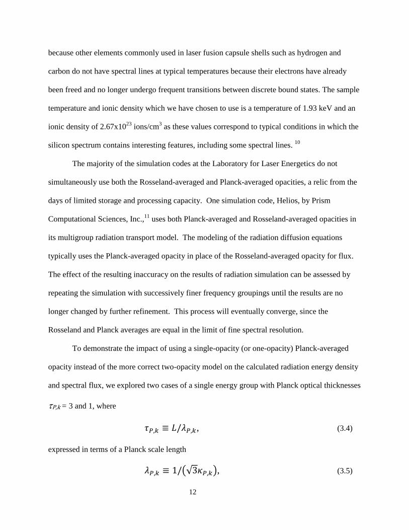
to illustrate what happens when the slab is of moderate optical thickness. Results are shown in

Fig. 2 for various ratios of the Rosseland-averaged opacity to the Planck-averaged opacity. In

these figures, x represents the position across the thickness of the slab, plotted as the

dimensionless quantity x/L, energy density is plotted in units of C0, and flux is plotted in units of

cC0.

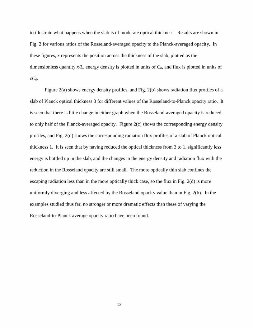
Figure 2(a) shows energy density profiles, and Fig. 2(b) shows radiation flux profiles of a

slab of Planck optical thickness 3 for different values of the Rosseland-to-Planck opacity ratio. It

is seen that there is little change in either graph when the Rosseland-averaged opacity is reduced

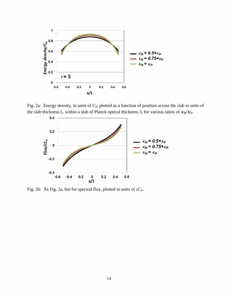
to only half of the Planck-averaged opacity. Figure 2(c) shows the corresponding energy density

profiles, and Fig. 2(d) shows the corresponding radiation flux profiles of a slab of Planck optical

thickness 1. It is seen that by having reduced the optical thickness from 3 to 1, significantly less

energy is bottled up in the slab, and the changes in the energy density and radiation flux with the

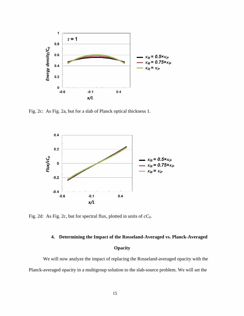
reduction in the Rosseland opacity are still small. The more optically thin slab confines the

escaping radiation less than in the more optically thick case, so the flux in Fig. 2(d) is more

uniformly diverging and less affected by the Rosseland opacity value than in Fig. 2(b). In the

examples studied thus far, no stronger or more dramatic effects than these of varying the

Rosseland-to-Planck average opacity ratio have been found.

14

Fig. 2a: Energy density, in units of C0, plotted as a function of position across the slab in units of the slab thickness L, within a slab of Planck optical thickness 3, for various ratios of κR/κP.

Fig. 2b: As Fig. 2a, but for spectral flux, plotted in units of cC0.

15

Fig. 2c: As Fig. 2a, but for a slab of Planck optical thickness 1.

Fig. 2d: As Fig. 2c, but for spectral flux, plotted in units of cC0.

4. Determining the Impact of the Rosseland-Averaged vs. Planck-Averaged

Opacity

We will now analyze the impact of replacing the Rosseland-averaged opacity with the

Planck-averaged opacity in a multigroup solution to the slab-source problem. We will set the

16

thickness of the slab to be 40 microns. The opacity, temperature, and ionic density are the same

as those used to create Figure 1.

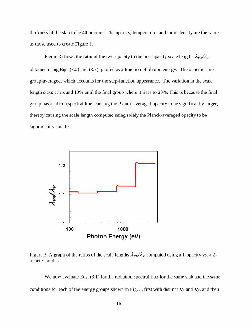
Figure 3 shows the ratio of the two-opacity to the one-opacity scale lengths λPR/λP

obtained using Eqs. (3.2) and (3.5), plotted as a function of photon energy. The opacities are

group-averaged, which accounts for the step-function appearance. The variation in the scale

length stays at around 10% until the final group where it rises to 20%. This is because the final

group has a silicon spectral line, causing the Planck-averaged opacity to be significantly larger,

thereby causing the scale length computed using solely the Planck-averaged opacity to be

significantly smaller.

Figure 3: A graph of the ratios of the scale lengths λPR/λP computed using a 1-opacity vs. a 2-opacity model.

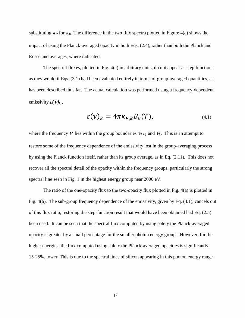
We now evaluate Eqs. (3.1) for the radiation spectral flux for the same slab and the same

conditions for each of the energy groups shown in Fig. 3, first with distinct κP and κR, and then

17

substituting κP for κR. The difference in the two flux spectra plotted in Figure 4(a) shows the

impact of using the Planck-averaged opacity in both Eqs. (2.4), rather than both the Planck and

Rosseland averages, where indicated.

The spectral fluxes, plotted in Fig. 4(a) in arbitrary units, do not appear as step functions,

as they would if Eqs. (3.1) had been evaluated entirely in terms of group-averaged quantities, as

has been described thus far. The actual calculation was performed using a frequency-dependent

emissivity ε(ν)k ,

𝜀(𝜈)𝑘 = 4𝜋𝜅𝑃,𝑘𝐵𝜈(𝑇), (4.1)

where the frequency ν lies within the group boundaries νk+1 and νk. This is an attempt to

restore some of the frequency dependence of the emissivity lost in the group-averaging process

by using the Planck function itself, rather than its group average, as in Eq. (2.11). This does not

recover all the spectral detail of the opacity within the frequency groups, particularly the strong

spectral line seen in Fig. 1 in the highest energy group near 2000 eV.

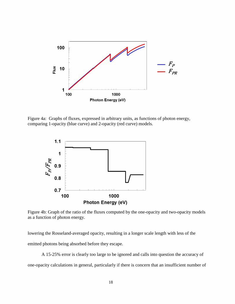
The ratio of the one-opacity flux to the two-opacity flux plotted in Fig. 4(a) is plotted in

Fig. 4(b). The sub-group frequency dependence of the emissivity, given by Eq. (4.1), cancels out

of this flux ratio, restoring the step-function result that would have been obtained had Eq. (2.5)

been used. It can be seen that the spectral flux computed by using solely the Planck-averaged

opacity is greater by a small percentage for the smaller photon energy groups. However, for the

higher energies, the flux computed using solely the Planck-averaged opacities is significantly,

15-25%, lower. This is due to the spectral lines of silicon appearing in this photon energy range

18

Figure 4a: Graphs of fluxes, expressed in arbitrary units, as functions of photon energy, comparing 1-opacity (blue curve) and 2-opacity (red curve) models.

Figure 4b: Graph of the ratio of the fluxes computed by the one-opacity and two-opacity models as a function of photon energy.

lowering the Rosseland-averaged opacity, resulting in a longer scale length with less of the

emitted photons being absorbed before they escape.

A 15-25% error is clearly too large to be ignored and calls into question the accuracy of

one-opacity calculations in general, particularly if there is concern that an insufficient number of

19

photon energy groups are being used. Our preliminary results suggest that upgrading a one-

opacity calculation to a two-opacity calculation may be an efficient complement to increasing the

accuracy of calculations by increasing the number of energy groups. This conclusion is based

only on our experience with the one example shown above. Before recommending that a

simulation code be upgraded to include a two-opacity model, other examples will have to be

studied, including realistic simulations of relevant experiments, as well as idealized

configurations in addition to the slab model considered here.

5. Conclusions

In conclusion, we have demonstrated, by example, the possible benefit of upgrading from

a one-opacity to a two-opacity model. Planck and interval-averaged opacities for Si were

obtained by running the Prism detailed atomic model in the code PROPACEOS. An analytic

solution was then derived for the radiation diffusion equation in a slab-source problem in which

either the same or separate opacities were used for absorption and transport, and the calculated

emitted spectral fluxes were compared. Even when the Planck and Rosseland averages differed,

the differences in flux were minimal except for spectral intervals where the optical depth was

approximately 1. There, it was shown that the values for flux can differ by ~10% - 20%. A

broad range of conditions with a larger set of test cases will be necessary to establish the

importance of changing from one-opacity to two-opacity modeling, but this work has laid some

of the groundwork for how this is to be done, particularly the solution to the slab problem

expressed in terms of both the Rosseland- and Planck-averaged opacities, which will allow a

20

broad range of cases to be considered. Thus far, it appears that upgrading to two-opacity

modeling merits serious consideration.

References

1. C. A. Haynam, P. J. Wegner, J. Auerbach, M.W. Bowers, S. N. Dixit, G. V. Erbert, G.

M. Heestand, M. A. Henesian, M. R. Hermann, K. S. Jancaitis, K. R. Manes, C.

D. Marshall, N. C. Mehta, J. Menapace, E. Moses, J. R. Murray, M. C. Nostrand,

C. D. Orth, R. Patterson, R. A. Sacks, M. J. Shaw, M. Spaeth, S. B. Sutton, W. H.

Williams, C. C. Widmayer, R. K. White, S. T. Yang, and B. M. Van

Wonterghem, Appl. Opt. 46, 3276-3303 (2007).

2. J. Nuckolls, L. Wood, A. Thiessen, and G. Zimmerman, Nature 239, 139 (1972); Lois

H. Gresh, Robert L. McCrory, and John M. Soures, Inertial Confinement Fusion:

An Introduction, Laboratory for Laser Energetics: Rochester, NY, 2009.

3. V. N. Goncharov, “Cryogenic Deuterium and Deuterium-Tritium Direct-Drive Implosions on

Omega,” in Laser-Plasma Interactions and Applications, Scottish Graduate Series 68,

Springer International Publishing, P. McKenna, D. Neely, R. Bingham, D. A.

Jaroszynski, eds., 2013.

4. T. R. Boehly, D. L. Brown, R. S. Craxton, R. L. Keck, J. P. Knauer, J. H. Kelly, T. J.

Kessler, S. A. Kumpan, S. J. Loucks, S. A. Letzring, F. J. Marshall, R. L.

McCrory, S. F. B. Morse, W. Seka, J. M. Soures, and C. P. Verdon, Opt.

Commun. 133, 495 (1997).

5. J. Delettrez, R. Epstein, M. C. Richardson, P. A. Jaanimagi, and B. L. Henke, Phys.

Rev. A 36, 3926 (1987).

6. R. Epstein, Equation of Transfer, privately circulated report, Laboratory for Laser

Energetics, Rochester, 2009.

21

7. S. Chandrasekhar, Radiative Transfer, Dover Publications, New York, 1960; J. I.

Castor, Radiation Hydrodynamics, Cambridge University Press, 2004.

8. G. C. Pomraning, The Equations of Radiation Hydrodynamics, Pergamon Press, Oxford,

1973.

9. H. R. Griem, Principles of Plasma Spectroscopy, Cambridge University Press,

Cambridge, England, 1997.

10. J. J. MacFarlane et al., PrismSPECT and SPECT3D Tools for Simulating X-ray, UV,

and Visible Spectra for Laboratory and Astrophysical Plasmas, American

Physical Society, 34th Meeting of the Division of Atomic, Molecular and Optical

Physics, May 2003; PrismSPECT, Prism Computational Sciences, Inc.,

http://www.prism-cs.com/

11. J. J. MacFarlane, I. E. Golovkin, P. R. Woodruff, J. Quant. Spectrosc. Radiat.

Transfer 99, 381-397 (2006).

Acknowledgements

Working at the Laboratory for Laser Energetics was one of the most memorable and

fulfilling experiences of my life. I would like to thank Dr. Craxton for running the high-school

intern program and extending me the opportunity to work at the Laboratory for Laser Energetics.

Dr. Reuben Epstein has my eternal gratitude for not only introducing me to the world of

scientific research with an interesting project, but also taking me under his wing in every way. I

would also like to thank my fellow interns for assisting me with various challenges along the

way. Finally, I would like to express my appreciation to all of my teachers, friends, and family

members for guiding me towards this path and supporting me in every endeavor.