The Vibratory Stress Relief Library - VSR Technology · VIBRATORY STRESS RELIEF OF MILD STEEL WELDMENTS S. Shankar B.S., Bangalore University, India, 1971 B.E., Indian Institute of

PH: 800.332.9770 FX: 888.964.3866

The

LibrarVibratory Stress Relief

y

REPRINT:

VIBRATORY STRESS RELIEF OF

MILD STEEL WELDMENTS

S. Shankar

A dissertation submitted to the faculty of Oregon Graduate Center in partial fulfillment of the requirements for the degree of Doctor of Philosophy

January, 1982

VIBRATORY STRESS RELIEF OF

MILD STEEL WELDMENTS

S. Shankar B.S., Bangalore University, India, 1971

B.E., Indian Institute of Science, India, 1974

A dissertation submitted to the faculty of the Oregon Graduate Center in partial fulfillment of the requirements for the degree

Doctor of Philosophy in

Materials Science

January, 1982

The dissertation "Vibratory Stress Relief of Mild Steel Weldments" by

S. Shankar has been examined and approved by the following Examination

Committee:

ii.

ACKNOWLEDGEMENTS

I wish to express my sincere thanks to Bob Turpin for assisting

in the fabrication of experimental set—up; to Nancy Christie and

Nancy Fick for typing; and to Barbara Ryall for her beautiful art

works.

Above all, I am very grateful to my research advisor, Professor

William E. Wood, for his support and guidance during the course of this

work.

iii.

iv. TABLE OF CONTENTS

Page ABSTRACT.......................................................... 1 OBJECTIVE......................................................... 2 CHAPTER 1—INTRODUCTION............................................ 4 CHAPTER 2—BACKGROUND ............................................. 7 2.1. Vibratory Stress Relief ................................. 7 2.2. Mechanism of Stress Relief by VSR........................ 9 2.3. Residual Stress Measurement Techniques................... 10 2.3.1. Sectioning Method ............................. 11 2.3.2. X—Ray Diffraction Method ...................... 12 2.3.3. Blind—Hole—Drilling Method .................... 13 2.4. Residual Stresses in Butt Welds.......................... 17 CHAPTER 3——EXPERIMENTAL........................................... 19 3.1. Material Selection....................................... 19 3.2. Weldment Preparation..................................... 19 3.3. Vibration Table Analysis................................. 22 3.4. VSR Treatment of Welded Specimens........................ 25 3.5. Residual Stress Measurement.............................. 27

3.5.1. Sectioning .................................... 11 3.5.2. X-Ray ......................................... 29 3.5.3. Blind—Hole—Drilling ........................... 29 3.6. Electron Microscopy...................................... 31 3.7. Mechanical Testing....................................... 32 3.7.1. Tensile Testing ............................... 32 3.7.2. Fatigue Testing ............................... 32

V. Page CHAPTER 4--RESULTS AND DISCUSSION................................. 35 4.1. Vibration Analysis....................................... 35 4.2. Residual Stress Analysis................................. 40

4.2.1. Verification of Longitudinal Residual Stress Pattern Developed in a Butt Weldment .......... 43 4.2.2. The Effect of Resonant Vibratory Treatment on the Longitudinal Residual Stress Distribution . 45 4.2.3. Effectiveness of the Vibratory Treatment on the Location of Weldments ......................... 65 4.2.4. The Effect of Frequency of Vibration on the Longitudinal Residual Stress Distribution ..... 66 4.2.5. Effect on Macrostresses ....................... 72 4.3. Microstructural Analysis................................. 76 4.4. Effect on Mechanical Properties.......................... 80 CHAPTER 5-—CONCLUSIONS............................................ 85 REFERENCES........................................................ 87 APPENDIX——Corrections for Blind—Hole—Drilling Analysis............ 90 Theoretical Analysis.......................................... 91 Practical Considerations...................................... 95 Experimental.................................................. 97 Discussion.................................................... 100 Machining Effect......................................... 100 Localized Plastic Flow Effect............................ 107 Recommendations .............................................. 112

vi.

LIST OF FIGURES Page

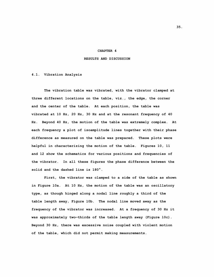
1. Variation of resolved stresses Sr and Sθ as a function of the distance r, from the hole edge, in a direction (a) parallel to the applied stress Sapp, θ = 0° and (b) at right angles to the applied stress, θ = 90° ................. 16 2. A schematic plot of longitudinal residual stress vs. distance from the weld center line. Sy is the yield stress of the base material ........................................ 18 3. Schematic of weld—joint preparation ......................... 21 4. Schematic of the tension plate weldment ..................... 23 5. Schematic showing the end view of the vibration table ....... 24 6. Schematic of the setup used for the vibrational analysis of table top ................................................ 26 7. Schematic of strain gauge layout in a SAE 1018 butt welded specimen used to verify the pattern of longitudinal residual stress distribution. Sectioning was done along the dotted lines ....................................................... 28 8. Schematic of the weldment used for sectioning ............... 30 9. Geometry of constant amplitude axial fatigue test specimen .. 33 10. Schematic showing (a) the position of vibrator on the table, (b) iso—amplitude lines at 10 Hz, and (c) iso—amplitude

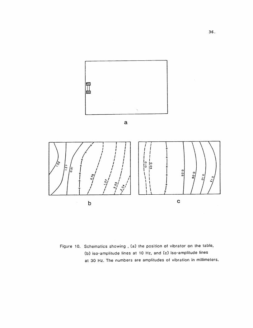
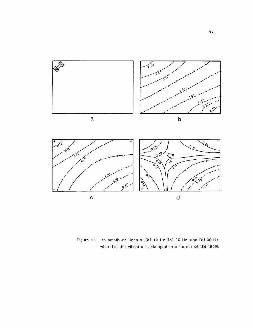
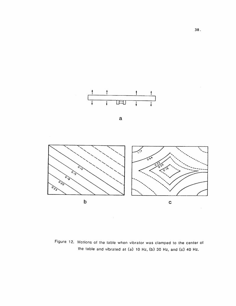
lines at 30 Hz. The numbers are amplitudes of vibration in millimeters ................................................. 36 11. Iso—amplitude lines at (b) 10 Hz, (c) 20 Hz, and (d) 30 Hz, when (a) the vibrator is clamped to a corner of the table ....................................................... 37 12. Motions of the table when vibrator was clamped to the center of the table and vibrated at (a) 10 Hz, (b) 30 Hz, and (c) 40 Hz ............................................... 38 13. Strain gauge rosette arrangement and the blind—hole geometry for determining residual stresses ..................... 41 14. Longitudinal residual stress distribution in a SAE 1018 butt weldment ............................................... 44

vii.

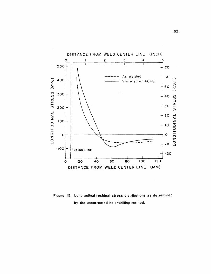
Page 15. Longitudinal residual stress distributions as determined by the uncorrected hole—drilling method ........................ 52 16. Residual stress distribution in a weldment vibrated at 40 Hz 63 17. The redistribution of longitudinal residual stresses as a result of the resonant vibratory treatment at 40 Hz ......... 64 18. The effect of frequency of vibration on the longitudinal residual stress distribution ................................ 71 19. Residual stress distribution in the unvibrated weldments showing excellent agreement between sectioning and corrected hole—drilling techniques .................................... 73 20. Residual stress distribution in the weldments vibrated at 40Hz ........................................................ 74 21. Transmission electron micrographs of the annealed A—36 mild steel samples ............................................... 78 22. Transmission electron micrographs of samples obtained from

the resonance vibration treated A—36 mild steel plate....... 79 23. S—N curve of fatigue samples from the unvibrated A—36 steel weldment .................................................... 81 24. S—N curve obtained from the fatigue samples of weldment treated at 30 Hz ............................................ 82 25. S—N curve obtained from the fatigue samples of resonant vibrated weldment ........................................... 83 APPENDIX Al. Strain gauge rosette arrangement and the blind—hole geometry for determining residual stresses ..................... 93 A2. Variation of the resolved stresses as a function of the distance from the hole edge ................................. 96 A3. Overestimation of the applied stress Sapp, due to localized yielding near the hole ............................ 98 A4. Schematic of the strain gauge layout on the test specimen ... 99 A5. Plot of average strain vs. applied stress for the parallel gauge ....................................................... 103

viii.

Page A6. Plot of average strain vs. applied stress for the transverse gauge ................................................. 104 A7. Variation of εM with the drilling clearance for the parallel gauge .............................................. 105 A8. Variation of εM with the drilling clearance for the transverse group ................................................. 106 A9. Plot of average strain vs. applied stress for parallel gauge ....................................................... 110 A10. Plot of average strain vs. applied stress for transverse gauge ....................................................... 111 A11. Percentage error in strain as a function of applied stress for a parallel gauge at various hole sizes .................. 113 A12. Percentage error in strain as a function of applied stress for a transverse gauge at various hole sizes ................ 114

ix.

LIST OF TABLES Page

I. CHEMICAL COMPOSITION (IN WT. PCT.) AND MECHANICAL PROPERTIES OF A—36 MILD STEEL ............................... 20 II. BLIND-HOLE—DRILLING STRESS ANALYSIS OF AS WELDED, UN— VIBRATED WELDMENTS (WITHOUT CORRECTION FACTORS) .............

Weldment #1................................................. 46

Weldment #2................................................. 47

Weldment #3................................................. 48 III. BLIND—HOLE—DRILLING STRESS ANALYSIS OF THE VIBRATED WELD— MENTS (WITHOUT CORRECTION FACTORS) ..........................

Weldment #1................................................. 49

Weldment #2................................................. 50

Weldment #3................................................. 51 IV. LONGITUDINAL RESIDUAL STRESSES IN THE VIBRATED SAMPLES AS DETERMINED BY THE SECTIONING TECHNIQUE ...................

Weldment #1................................................. 53

Weldment #2................................................. 54

Weldment #3................................................. 55 V. BLIND—HOLE-DRILLING STRESS ANALYSIS OF AS WELDED, UNVI- BRATED WELDMENTS (WITH CORRECTION FACTORS)..................

Weldment #1................................................. 57

Weldment #2................................................. 58

Weldment #3................................................. 59 VI. BLIND—HOLE—DRILLING STRESS ANALYSIS OF THE VIBRATED WELDMENTS (WITH CORRECTION FACTORS) .........................

Weldment #1................................................. 60

Weldment #2................................................. 61

Weldment #3................................................. 62

x.

Page

VII. RESIDUAL STRESS ANALYSIS BY THE SECTIONING TECHNIQUE (GAUGE FACTOR = 2.04 FOR ALL THE STRAIN GAUGES) ...........

As welded, control weldment ............................... 68

Weldment vibrated at 30 Hz ................................ 69

Weldment vibrated at 40 Hz ................................ 70 VIII. RESIDUAL STRESSES IN THE TENSION WELDMENT AS DETERMINED FROM THE CORRECTED HOLE—DRILLING TECHNIQUE ................ 75

IX. EFFECT OF THE FREQUENCY OF VIBRATION ON THE MECHANICAL PROPERTIES OF A—36 STEEL BUTT WELDS ....................... 84 APPENDIX A—I. VARIATION OF AVERAGE STRAIN WITH APPLIED STRESS FOR GAUGE #1, WHICH IS PARALLEL TO THE APPLIED STRESS, θ = 0° . SPECIMEN #1 ................................................ 101 A—II. VARIATION OF AVERAGE STRAIN WITH APPLIED STRESS FOR GAUGE #3, WHICH IS TRANSVERSE TO THE DIRECTION OF APPLIED STRESS, θ = 90°, SPECIMEN #1 ............................... 102 A—III. VARIATION OF AVERAGE STRAINS RECORDED FROM GAUGE #1 AS A FUNCTION OF APPLIED STRESS FOR VARIOUS HOLE SIZES. SPECIMEN #2 ................................................ 108 A—IV. VARIATION OF AVERAGE STRAINS RECORDED FROM GAUGE #3 AS A

FUNCTION OF APPLIED STRESS FOR VARIOUS HOLE SIZES. SPECIMEN #3 ................................................ 109 A—V. MODIFICATION OF RELAXED STRAINS OF ROSETTE #1, WELDMENT #1, TO ACCOUNT FOR THE DRILLING ERROR AND THE ERROR DUE TO LOCAL YIELDING .......................................... 116

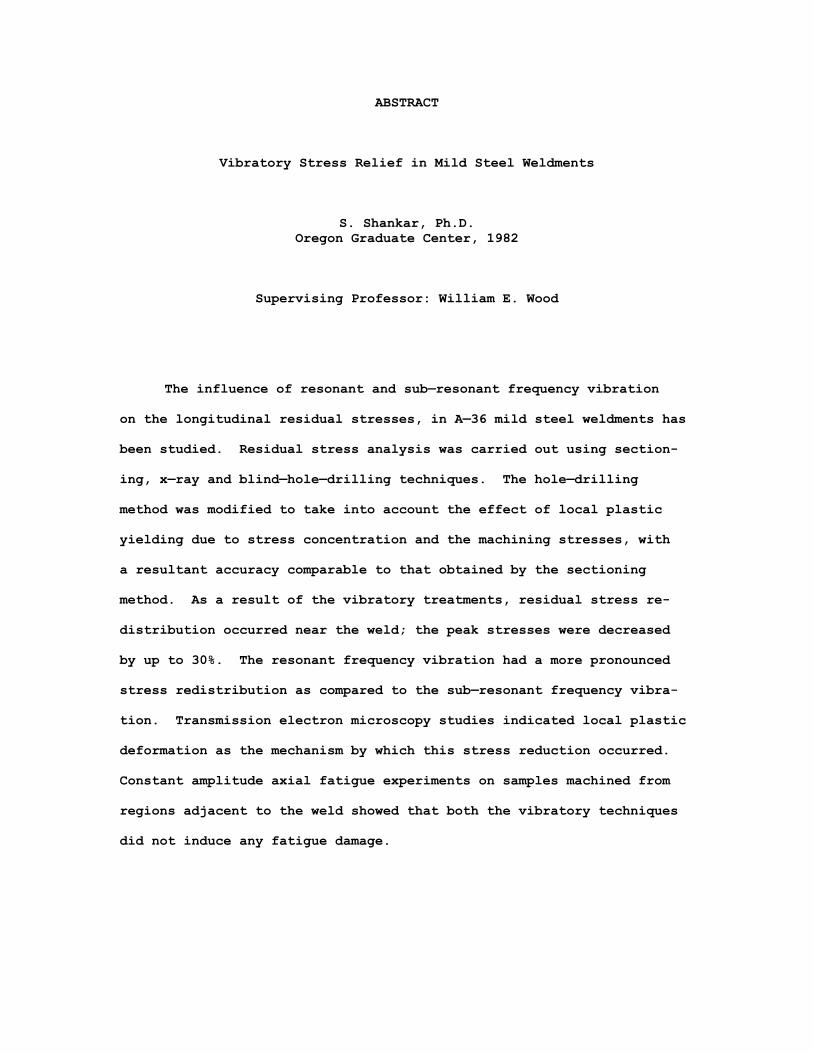
ABSTRACT

Vibratory Stress Relief in Mild Steel Weldments

S. Shankar, Ph.D. Oregon Graduate Center, 1982

Supervising Professor: William E. Wood

The influence of resonant and sub—resonant frequency vibration

on the longitudinal residual stresses, in A—36 mild steel weldments has

been studied. Residual stress analysis was carried out using section-

ing, x—ray and blind—hole—drilling techniques. The hole—drilling

method was modified to take into account the effect of local plastic

yielding due to stress concentration and the machining stresses, with

a resultant accuracy comparable to that obtained by the sectioning

method. As a result of the vibratory treatments, residual stress re-

distribution occurred near the weld; the peak stresses were decreased

by up to 30%. The resonant frequency vibration had a more pronounced

stress redistribution as compared to the sub—resonant frequency vibra-

tion. Transmission electron microscopy studies indicated local plastic

deformation as the mechanism by which this stress reduction occurred.

Constant amplitude axial fatigue experiments on samples machined from

regions adjacent to the weld showed that both the vibratory techniques

did not induce any fatigue damage.

2.

OBJECTIVE

Vibratory methods have been used for the last several decades to

modify internal stresses in castings, forgings and welded structures.

In recent years, a process called vibratory stress relief (VSR) has

been applied with increasing success to attain shape stabilization and

to control distortion. Attempts to use VSR methods for stress relief

or stress redistribution to guard against service failures such as

fatigue and stress corrosion cracking have met with limited success.

Although to date several studies have shown that vibrations do change

residual stresses, there have been few fundamental studies undertaken

to establish the mechanism(s) by which vibratory methods alter the

residual stresses during welding. The lack of fundamental analysis

combined with suggested operating practices that were contradictory in

nature has increased the skepticism about the success of the technique

in reducing residual stresses. A better understanding of the process

in terms of its mechanism(s) together with the attendant effects is

essential if VSR is to be used as a viable technique for altering

residual stresses.

The objectives of this investigation were to study:

1. The conditions under which VSR works;

2. The effect of VSR on residual stresses and the extent

of stress relief;

3.

3. The mechanism(s) by which VSR brings about the stress

relief; and finally,

4. Whether or not VSR causes fatigue damage.

4.

CHAPTER 1

INTRODUCTION

Residual stresses are of concern to producers and users of all

types of machinery and structures and may cause dimensional instabil-

ity during machining, contribute to low—stress brittle fracture and

reduce fatigue strength. Those who make and use welded fabrications

must be particularly concerned with the effects of residual stresses

because of the relatively high residual stress levels inherently

produced with most common welding processes.

When it is desired to reduce residual stresses in a fabrication

to as low a level as possible, the most widely used and successful

method is thermal stress relief. Specifying temperature, time and heat-

ing and cooling rates are all that is usually necessary to guarantee

reduction of residual stresses to reliably low levels throughout a

fabrication.

Thermal stress relief, however, can have certain adverse effects

such as scaling, discoloration, loss of finish, distortion, metal-

lurgical changes in the microstructure, etc. It is also, in some

instances, time consuming and, with increasing energy costs, very

expensive. Since residual stresses are developed to some degree in

virtually every machining operation, there are many situations where

it would be advantageous to stabilize the part at several stages of

fabrication. Thermal cycling would be impractical in these cases.

5.

Also, large components like gas storage tanks, bridge structures, and

rail car panels are impossible or impractical to stress relieve by

thermal treatments. In this background, an alternative technique of

stress relief 1,2 that employs mechanical vibration, has emerged.

This process is called vibratory stress relief (VSR) or vibratory

metal stabilization (VMS). Over the last fifteen years, this method

of stress relief has evolved from a little—known art into a basic

process, and one which for some industries is now well tried and

established as an alternative to thermal treatment for stabilizing

castings, fabrications, and bar components. 3-5

The major interest in vibrational stress relief has been its

relative simplicity compared with thermal stress relief. For instance,

compared with thermal stress relief equipment commercially available,

vibratory stress relief equipment is far less expensive, requires con-

siderably less time for the stress relief treatment, is more portable,

generally occupies less floor space, and causes no oxide scale forma—

tion. However, there is little experience in predicting the effect-

iveness of the treatment and there is little quantitative information

on the effectiveness, use, or magnitude of any effects and the mechan-

ism involved. In the absence of such quantitative information, it is

difficult to determine when and where vibratory stress relief may be

effectively applied, particularly in massive complex fabrications.

The present study was undertaken to provide some quantitative

data on the vibratory stress relief process applied to A—36 mild

steel butt welds. The various phases of this study focused on the

6.

analysis of vibration, residual stress analysis using sectioning,

x—ray and blind—hole—drilling techniques, and the effect of vibration

on the microstructure and the mechanical properties of the weldments.

This comprehensive study is unique in that it combines vibration

methodology, residual stress analysis, microstructural analysis,

and mechanical testing.

7.

CHAPTER 2

BACKGROUND

2.1. Vibratory Stress Relief

Vibration, in its various forms, has been used to stabilize parts

for many years. For example, in the ancient art of “hammer anneal-

ing,” a high amplitude, gradually decaying vibration was induced by

repeated hammer blows. Large castings, at one time, were stabil-

ized by dropping them from a considerable height into a pile of sand.

In the “natural aging” process, the workpieces were stored outdoors

for a considerable period of time. The metal expanded and contracted

with changes in ambient temperature at a very low frequency of

one cycle per day. The nature of the vibrations produced in these

methods made them uncontrollable, unpredictable, and too slow. Gradual

experimentation to make the process more repeatable by the control and

monitoring of vibrations used has paved the way to the state—of—the—

art vibratory stress relief techniques.

The actual process of vibratory stress relief is simple and con-

sists of inducing a metal structure to be stabilized into one or more

resonant or sub—resonant vibratory states using high force exciters.

Vibrational stress relief equipment commercially available generally

consists of a variable—speed motor driving eccentric weights (also

known as the vibrator) and its associated power supply and control

equipment.

8.

The vibrations can be imparted to the workpiece in two ways.

If the structure is sufficiently large, the vibrator can be clamped

directly to it and the motor energized to vibrate the workpiece. The

workpiece is isolated from the ground by supporting on rubber or foam

pads, so that the vibrations are not lost or taken up by the support-

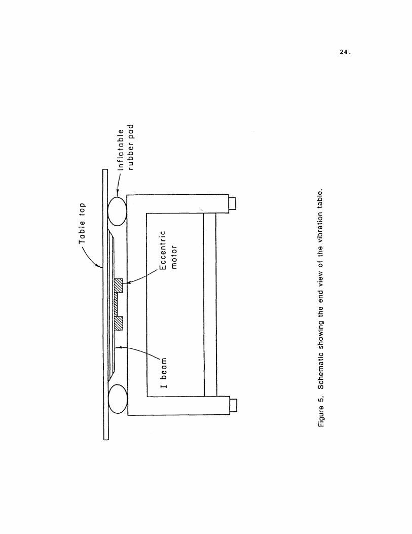
ing structure. Another way of imparting vibrations utilizes a special

vibration table. Here the vibrator is attached to the table top which

is freely suspended on inflatable rubber pads. The workpiece is

clamped to the top of the table and the motor energized to vibrate

the table and, hence, the workpiece. Small parts, whose natural fre-

quencies lie outside the range of the vibrator, can be effectively

treated using the vibration table. By combining the small workpiece

with the table, the natural frequencies of the entire combination can

be brought down to be successfully vibrated. An accelerometer

clamped to the structure or the table is used to find the natural

frequencies. The frequency of vibration depends upon the material of

the workpiece, its size and shape. In general, the frequencies

encountered are less than 100 Hz. The vibratory treatment itself is

short, usually less than 30 minutes.

Currently, there are two types of vibratory treatment in practice.

In the first type, the unit is attached to the structure and is

energized and scanned very slowly from zero to its maximum

frequency (e.g., 0—100 Hz in about 8 minutes). The response of the

structure is monitored and the resonant frequencies noted. Usually

two or three such frequencies exist. The vibrator is then turned off

9.

and returned to a speed that corresponds to the first low resonant

frequency of the structure. The vibration is allowed to continue for

a given length of time (usually about 10 minutes), at the end of

which the frequency is slowly ramped out of the resonant condition

until the next higher resonant frequency is found and the process is

repeated.

In the second type of vibratory technique, after the initial

scanning to determine the resonant frequencies, the vibration is held

at frequencies just below each resonant frequency. Usually, the work—

piece is vibrated at a frequency 10 Hz below the resonant frequency.

One aspect of this study deals with the effectiveness of these two

practices.

2.2. Mechanism of Stress Relief by VSR

During a thermal stress relief treatment, the yield point of the

material is substantially lowered, allowing the stresses (which may

now well exceed the new, high temperature yield point) to cause

plastic flow and reduce the level of residual stresses. However,

the mechanism of stress relief by vibration is not fully understood.

Currently, there are two major hypotheses proposed to explain the

mechanism of stress relief by vibration. One hypothesis draws an

analogy between stress relief by vibration and by heat treatment by

relating it to the displacements of the atoms that build up the

crystal lattice. 1,31-33 The low—frequency vibrations are supposed to

impart sufficient energy to the atoms to enable them to take up new

10.

positions. This theory based on internal friction can presumably

be applied to materials that display a pronounced tendency towards

natural aging. However, there seems to be no experimental evidence

to support this conjecture.

The other hypothesis attributes the stress relief due to the

process of plastic deformation. 34’35 Unlike the previous supposition,

a number of experimental investigations 36-40 have shown that during

vibrational treatments, the combined residual and cyclic stresses

exceed the yield point of the material, resulting in residual stress

reduction by plastic deformation. However, none of these investiga-

tions presented direct observations of plastic deformation.

In the present investigation, an attempt is made to document

the occurrence of plastic deformation in the vibrational treatments.

2.3. Residual Stress Measurement Techniques

An accurate assessment of the efficiency of any stress relief

treatment involves measurement of residual stresses before and after

the treatment, and virtually every conceivable method of monitoring

displacements has been employed. For ease of reference these can be

classified into the following groups:

1. Mechanical

2. Moiré and associated techniques

3. X-ray

4. Ultrasonic

5. Magneto—elastic

6. Analytical

11.

A complete summary of all the published literature on this subject has

been adequately covered in reviews. 6-8

By far the most practical, well—developed, and hence widely

used techniques are sectioning, blind—hole—drilling (both mechanical

types), and x—ray. In the present study, the first two methods were

widely used, together with x—rays (to a limited extent), for

residual stress analysis. Since accurate residual stress analysis

is a key part of this investigation, and a shortcoming of many previ-

ous studies, a brief description of the methodology, merits, and

shortcomings of these three techniques are outlined in the following

sections.

2.3.1. Sectioning Method

All mechanical techniques involve some degree of destruction. In

particular, the sectioning technique is completely destructive and

herein lies its major disadvantage. This method has been success-

fully applied to accurately measure uniaxial and biaxial states of

stress and to a limited extent triaxial residual stress. The method

consists in carefully sectioning the workpiece in which residual

stresses are to be determined into smaller strips and measuring the

change in strain in each individual strip. The series of strains

thus measured gives the stress distribution in the entire workpiece,

using the formula σ = Eε. The actual geometry of slicing and the

formulae to be used depend on specific situations. 9,10 The method, apart

from being destructive, is very time consuming since the cutting

12.

process should be done slowly, cooling the specimen with a jet of

coolant to ensure that cutting in itself does not produce any strains.

In the present investigation the accuracy of the sectioning tech-

nique used was about ± 3.5 MPa in mild steel samples. Due to this

high accuracy of stress measurement, the sectioning technique was

used as a standard against which the other stress measurement tech-

niques were compared.

2.3.2. X—Ray Diffraction Method

The x—ray diffraction procedure for determining the surface

residual stresses is well established.10-12 The fundamental theory

of stress measurement by means of x—rays is based on the fact that

the interplanar spacing of the atomic planes within a specimen is

changed when subjected to stress. A change ∆d hkℓ, in the interplanar

spacing dhkℓ will cause a corresponding change, ∆θ, in the Bragg

angle of diffraction by the family of planes. The strain ∆d/d can

be measured by the change in the diffraction angle and the stress

can be obtained from the strain with formulae derived from linear

isotropic elastic theory.

In practice the angle of diffraction of x—rays is measured

either by a back reflection camera or by a suitable diffractometer,

with a maximum accuracy of the order of ± 0.02 degree. 13 This means

that the value of the lattice spacing can be determined to an accuracy

of the order of ± 0.0002 Ǻ, which in turn allows the calculation of

the residual stresses to ± 14 MPa. Thus the x—ray technique has less

13.

accuracy than the sectioning method. Further, additional errors due

to instrument misalignment and uncertainty in the elastic constants

can bring the total error to ± 34.5 MPa which is about 12% in mild

steels. The x—ray technique is designed for the measurement of

macrostresses, but microresidual stresses (due to inhomogeneities

in the microstructure) can also be detected by x—rays and these

can interfere with the accuracy of the data. Thus, in some

materials, including plastically deformed steel, interpretation

of the results may be difficult.

However, it is completely non—destructive and determines the

total elastic stress present in the sample for a given location and

direction independent of the sample geometry without relaxing the

stress being measured. Another advantage of this technique is that

the area over which the stress is averaged can be varied by limiting

the size of the x—ray beam. Using a small beam size (typically of

the order of 2 x 2 mm), localized stresses adjacent to welds or

fasteners can be measured.

2.3.3. Blind—Hole—Drilling Method

It is possible to determine residual stresses by drilling a hole

in a specimen and measuring the resulting change of strain in the

vicinity of the hole. 14-17 This method, also known as hole—

relaxation or hole—drilling method, is the least destructive of the

mechanical methods. A hole of only a few millimeters in diameter and

14.

depth may suffice for the stress measurement. Since this amount of

destruction can sometimes be tolerated, the method is semidestructive

in nature. It is a very simple and economical method and can be used

to measure stresses over a very small area in a very short period of

time.

In actual practice, a strain gauge rosette which is commercially

available is bonded to the specimen with the center of the rosette

coinciding with the point where stresses are to be measured. A hole

is then drilled at the center of the rosette. From the strain read-

ings taken before and after the drilling of the hole, the principal

stresses in the plate before the hole was drilled is computed.

Both uniaxial and biaxial stresses can be measured with this tech-

nique.18 The principle of this technique is based on the work of

Kirsch 19 on the stress distribution around a circular hole in a

plate subjected to unidirectional tension. By superposition, the

same principle can be extended to biaxial stress fields. 15—17

The relaxed strains measured by the gauges on the surface of the

structure are dependent on the depth of hole until this exceeds a

dimension where strain changes do not affect the surface. It has

been very clearly shown 17,18,21,22 that full relaxation is obtained

at the surface for a depth equal to the hole diameter. Thus, in

practice, where the components of interest are usually thick compared

with the hole diameter, blind holes are formed; hence the name blind—

hole—drilling.

It is imperative that the method employed to form the hole should

not introduce any stresses. The rotating cutters or end mills commonly

15.

employed to drill the hole can introduce appreciable stresses.21-23

An alternate technique of hole formation, viz., airbrasive 24 or abra-

sive jet 21 machining seems to be very effective and the machining

strains measured are well within the accuracy of the strain recording

equipment. However, not only is the equipment used in this method

very expensive but the method itself is more time consuming to drill

a hole of given size and in part to handle the ancillary equipment. 23’24

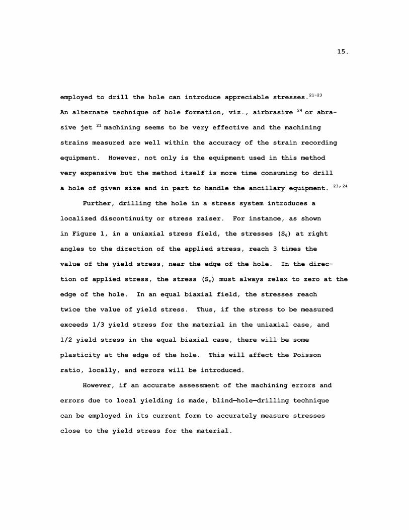
Further, drilling the hole in a stress system introduces a

localized discontinuity or stress raiser. For instance, as shown

in Figure 1, in a uniaxial stress field, the stresses (Sθ) at right

angles to the direction of the applied stress, reach 3 times the

value of the yield stress, near the edge of the hole. In the direc-

tion of applied stress, the stress (Sr) must always relax to zero at the

edge of the hole. In an equal biaxial field, the stresses reach

twice the value of yield stress. Thus, if the stress to be measured

exceeds 1/3 yield stress for the material in the uniaxial case, and

1/2 yield stress in the equal biaxial case, there will be some

plasticity at the edge of the hole. This will affect the Poisson

ratio, locally, and errors will be introduced.

However, if an accurate assessment of the machining errors and

errors due to local yielding is made, blind—hole—drilling technique

can be employed in its current form to accurately measure stresses

close to the yield stress for the material.

16.

Figure 1. Variation of resolved stresses Sr and Sθ as a function of

the distance r, from the hole edge in a direction (a) parallel

to the applied stress Sapp, θ = 0° and (b) at right angles to

the applied stress, θ 90°.

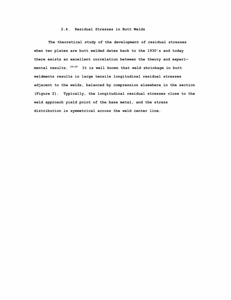
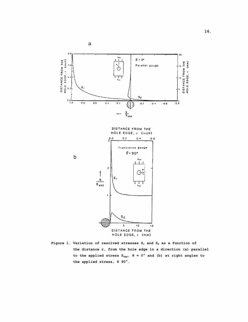
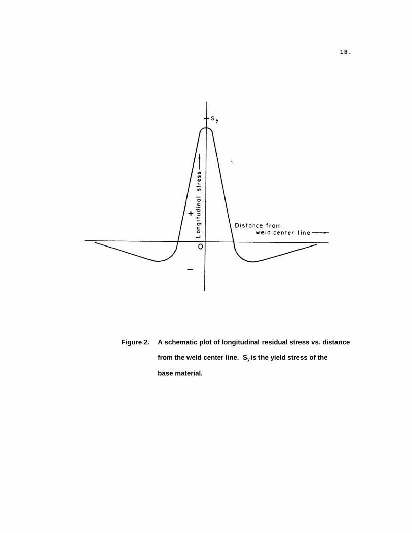
2.4. Residual Stresses in Butt Welds

The theoretical study of the development of residual stresses

when two plates are butt welded dates back to the 1930’s and today

there exists an excellent correlation between the theory and experi—

mental results. 25—29 It is well known that weld shrinkage in butt

weldments results in large tensile longitudinal residual stresses

adjacent to the welds, balanced by compression elsewhere in the section

(Figure 2). Typically, the longitudinal residual stresses close to the

weld approach yield point of the base metal, and the stress

distribution is symmetrical across the weld center line.

18.

Figure 2. A schematic plot of longitudinal residual stress vs. distance

from the weld center line. Sy is the yield stress of the

base material.

19.

CHAPTER 3

EXPERIMENTAL

3.1. Material Selection

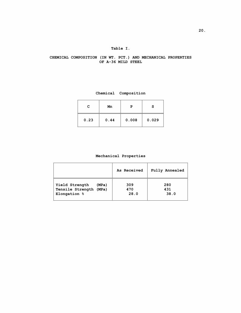
In this investigation, mill plates of ASTM designation A—36

constructional steel were used. The chemical composition of the as—

received steel is given in Table I. All the plates used to make the

butt weldments were first annealed to completely relieve the as—

received residual stresses. The annealing treatment consisted of

heating the plates for one hour at 870°C in an inert atmosphere,

furnace cooling to 540°C and then air cooling to the room temperature.

The tensile properties of the as—received and the annealed A—36 steel

are also shown in Table I. Two SAE 1018 steel plates were also given

the previous annealing treatment.

3.2. Weldment Preparation

In order to verify and confirm the pattern of longitudinal

residual stress distribution in a butt welded sample, the annealed

SAE 1018 steel plates, each 305 x 102 x 6.4 mm, were butt welded using

3.2 mm E—7024 electrode. No weld joint preparation was made.

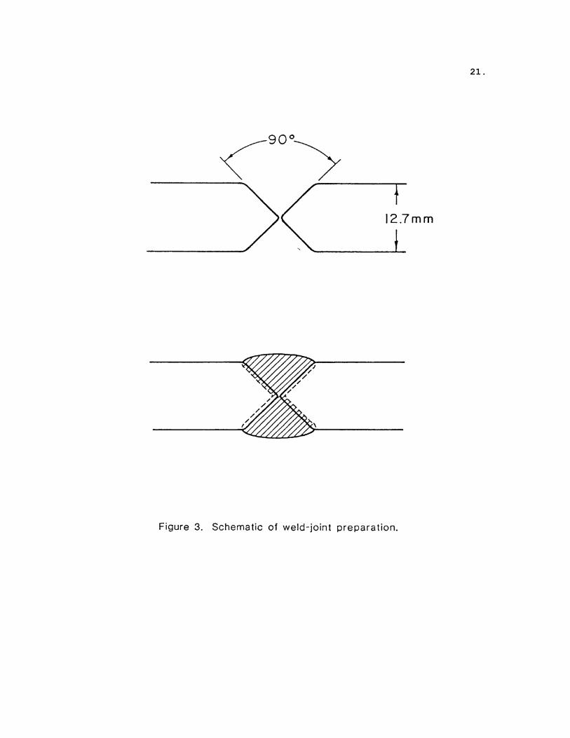
The annealed A—36 steel plates were butt welded using 4 mm

E—6013 electrodes. The weld joint preparation is shown in Figure 3.

Double—vee bevels were used to minimize the distortion and to ensure

20.

Table I.

CHEMICAL COMPOSITION (IN WT. PCT.) AND MECHANICAL PROPERTIES OF A-36 MILD STEEL

Chemical Composition

C Mn P S

0.23 0.44 0.008 0.029

Mechanical Properties

As Received Fully Annealed

Yield Strength (MPa) Tensile Strength (MPa) Elongation %

309 470

28.0

280 431

38.0

21.

22.

uniform through thickness stress distribution in the weldment.30

Distortion was further reduced by clamping the plates by the edge.

The clamping was such that the lateral motion of the plates was

unhindered during welding which would result in low values of trans-

verse stresses. A total of six butt welds were made of which three

were 914 x 406 x 12.7 mm and the other three were 305 x 508 x 12.7 mm

in size.

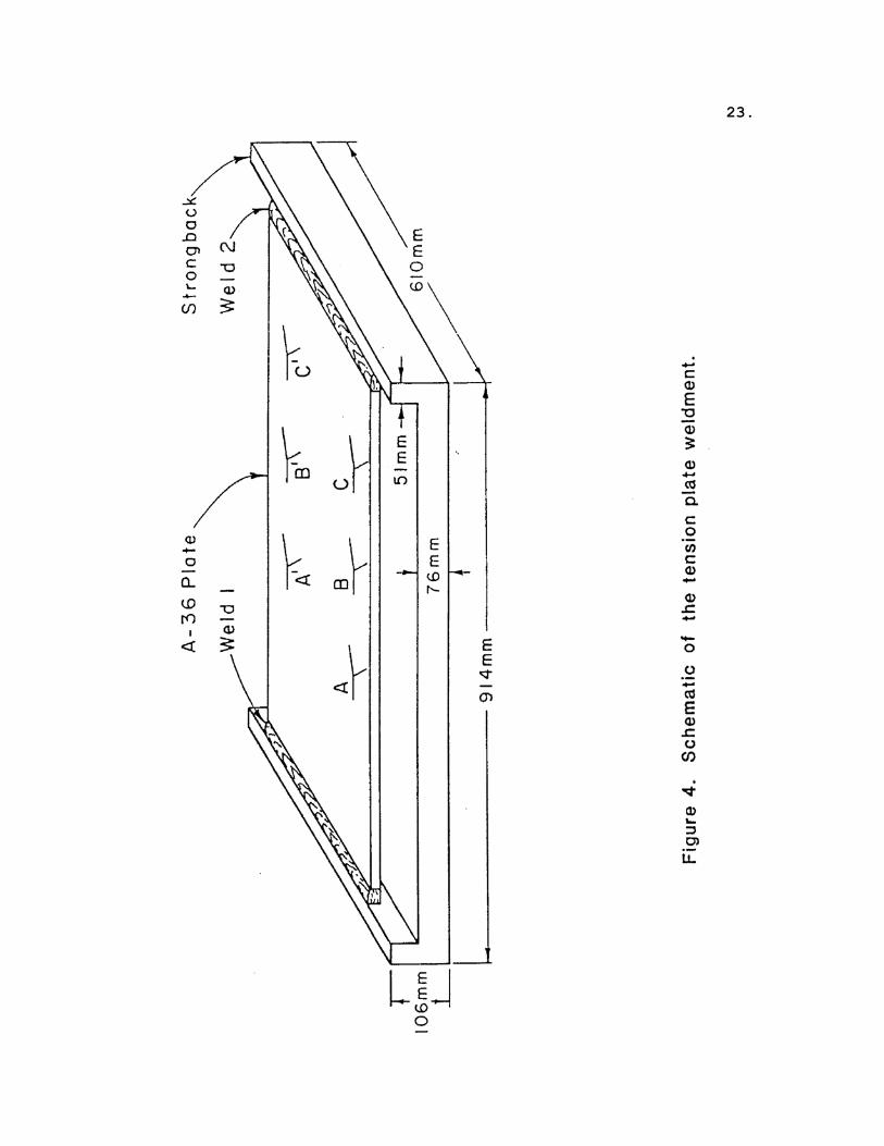
In order to study the vibratory stress relief of a heavy struc-

ture without using the vibration table, the following tension weldment

was prepared (Figure 4). An annealed A—36 mild steel plate 762 x 457

x 19 mm was first welded along weld 1 to a strongback with about

12.5 mm clearance between the two. The plate was then heated to

about 143°C and while still hot, was welded along weld 2 to the

strongback. The plate, on cooling, contracts and develops uniform,

yield point magnitude tensile stresses sufficiently removed from the

welded ends.

3.3. Vibration Table Analysis

The vibratory treatments were carried out using a vibration table

(Figure 5). The table top was 1830 x 1219 x 25.4 mm aluminum alloy

plate, braced rigidly by several steel I beams. It was mounted on

four inflatable rubber pads which helped to isolate the table from

the ground during vibrating. The vibrations were produced by a bottom

center bolted DC motor containing eccentric weights mounted on each

end of its shaft.

23.

24.

25.

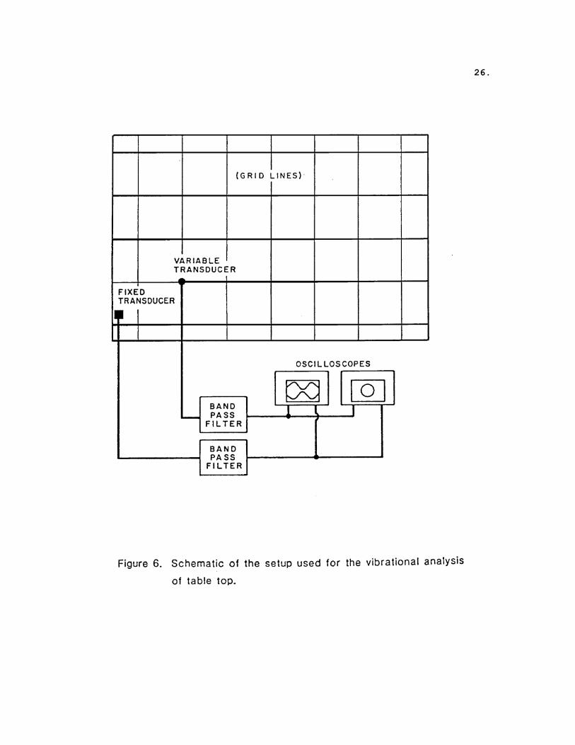
Grid lines 254 mm apart crisscrossed the surface of the table.

The motor was energized to selected frequencies up to 40 Hz, and at

each frequency the amplitude of vibration and the phase difference of

the amplitudes were measured at the intersecting points of grid lines.

A schematic of the setup used to monitor the vibrations is shown

in Figure 6. Two sensitive piezoelectric transducers, one fixed and

the other movable, were used to monitor the amplitudes and phase

differences. Filters were used to obtain a clear sinusoidal signal

free from higher harmonics and interfering waves from the boundaries

of the table.

3.4. VSR Treatment of Welded Specimens

The weldments were subjected to vibratory stress relief treat-

ment by bolting rigidly to the vibration table. A good mechanical

contact was necessary to efficiently transfer vibrations from the

table to the weldment. The duration of the vibratory treatment was

a fixed time of 20 minutes, and the resonant frequency was maintained

manually.

The effect of weldment location on the vibration table was studied

using the three 305 x 508 x 12.7 mm weldments. Of the three

weldments, one was vibrated by clamping to the center of the table

and the other two at two corners of the table. The frequency of

vibration in all the three cases was 40 Hz.

Additionally, the effect of frequency of vibration treatment was

studied using the three 914 x 406 x 12.7 mm weldments. One

26.

27.

weldment was vibrated at 40 Hz, the second at 30 Hz and the third was

not vibrated and was used as a control.

The 400 kg weldment shown in Figure 4 was vibrated by clamping

the vibrator directly to it. The frequency of vibration was 37 Hz,

a fundamental vibrational frequency of the assembly. The weldment

and the vibrator assembly were placed on heavy duty rubber pads to

isolate the workpiece. The duration of treatment was 20 minutes.

3.5. Residual Stress Measurement

Residual stresses in weldments were determined by sectioning,

x—ray, and blind—hole—drilling techniques.

3.5.1. Sectioning

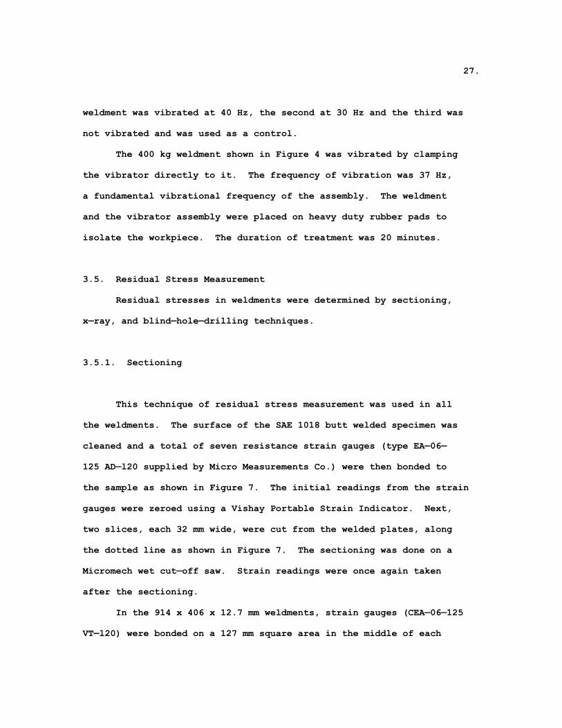
This technique of residual stress measurement was used in all

the weldments. The surface of the SAE 1018 butt welded specimen was

cleaned and a total of seven resistance strain gauges (type EA—06—

125 AD—l20 supplied by Micro Measurements Co.) were then bonded to

the sample as shown in Figure 7. The initial readings from the strain

gauges were zeroed using a Vishay Portable Strain Indicator. Next,

two slices, each 32 mm wide, were cut from the welded plates, along

the dotted line as shown in Figure 7. The sectioning was done on a

Micromech wet cut—off saw. Strain readings were once again taken

after the sectioning.

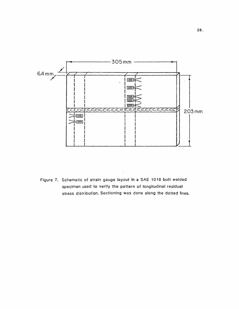
In the 914 x 406 x 12.7 mm weldments, strain gauges (CEA—06—125

VT—l20) were bonded on a 127 mm square area in the middle of each

28.

29.

weldment (Figure 8). This square region was then sectioned off using

a saw mill operating at a slow speed. Care was taken not to heat the

area by directing a jet of coolant at the cutting edge of the saw

blade. Strain, as well as resistance, measurements were made from

these strain gauges before and after sectioning. A Vishay 1011 port-

able strain indicator together with a Vishay 1012 portable switch and

balance unit were used for strain measurements. Resistances from the

strain gauges were measured using a standard potentiometer.

In the 305 x 508 x 12.7 mm samples used for the blind—hole—

drilling experiments, sectioning technique was employed as a check for

the residual stresses measured after vibration. In these samples a

strip 25.4 mm wide was cut across the weld.

3.5.2. X-Ray

Further measurements of residual stresses, using an x—ray method,

were made in the 127 mm square pieces obtained from the sectioning

technique. The sin2ψ technique13 employed for residual stress meas-

urement used six ψ angles at equal values of sin2 ψ from ψ = 0 to ψ =

45 degrees.

3.5.3. Blind—Hole—Drilling

Residual stresses in the 305 x 508 x 12.7 mm weldments were

determined by the blind—hole—drilling technique. Strain gauge ros—

ettes (type EA—06—125 RE—120 supplied by Micro Measurements Co.) were

bonded at predetermined locations on either side of the weld. Before

30.

31.

vibrating each weldment, holes approximately 3 mm in diameter and

depth were drilled at the center of rosettes mounted on one side of

the weld to determine the residual stresses in the as—welded condi-

tion. The weldments were then individually vibrated at 40 Hz for 20

minutes by clamping them at several locations on the vibration

table. Holes were again drilled in the rosettes on the other side

of the weld to obtain the residual stress distribution after vibra-

tion. A Photolastic model RS—200 milling guide was used to align

the drill bit exactly at the center of the rosette and also to rigidly

guide the drill bit to produce consistently straight, true, and clean

holes.

The blind—hole—drilling technique was also employed to determine

the effect of vibratory treatment on the residual stresses in the

tension plate of Figure 4. Residual stresses before vibration were

determined using the strain gauge rosettes at A, B and C. After the

vibratory treatment the residual stresses were again measured using

rosettes A’, B’ and C’.

3.6. Electron Microscopy

In order to detect the evidence of plastic deformation, 1 mm

thick coupons were sectioned off from the 19 mm A—36 tension plate.

These coupons were cut from areas 13 mm around the rosettes. They

were then ground on abrasive wheels to a thickness of 0.25 mm.

Further thinning to about 75 microns was done by electrolytic polish-

ing. Disks of about 3 mm in diameter were punched out carefully for

32.

jet polishing. Both the electrolytic and the jet polishing were done

at about 5°C in a solution of 135 cc of glacial acetic acid, 25 g of

chromium trioxide and 7 cc of distilled water. The samples were

studied in a Hitachi HU—11B3 electron microscope at an operating

voltage of 125 kV.

3.7. Mechanical Testing

Tensile and fatigue experiments were carried out using the

samples machined out of the three 914 x 406 x 12.7 mm weldments. A

10,000 kg Instron Lawrence dynamic test system was used for all test-

ing. The samples were sectioned off of regions 12.7 mm from either

side of the weld center line. A total of 4 tensile and 16 fatigue

samples from each of the three weldments were tested.

3.7.1. Tensile Testing

Tensile bars of 6.35 mm diameter were machined according to the

ASTM specification A370—77. Testing was carried out at a crosshead

speed of 1 mm/minute. Strain was measured with a strain gauge

extensometer.

3.7.2. Fatigue Testing

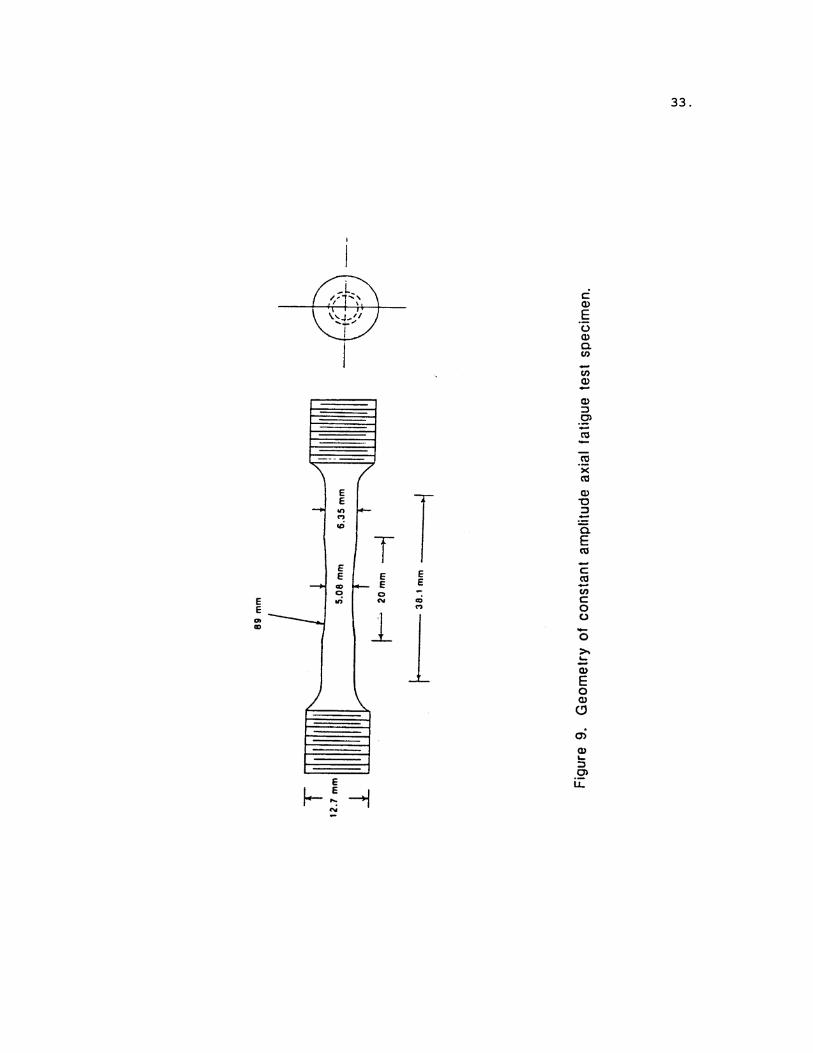
Constant amplitude axial fatigue tests were conducted using

5.08 mm diameter fatigue samples satisfying the ASTM specification

E466—76 (Figure 9). The surface of all the samples was finely

polished using a 600 grit emery cloth. The tests were performed in

33.

34.

air at room temperature at a frequency of 30 Hz and with an R ratio

of 0.1. Samples that did not fail after l07 cycles were reused again

at higher stress levels. This method of testing is known as the

staircase fatigue testing.

35.

CHAPTER 4

RESULTS AND DISCUSSION

4.1. Vibration Analysis

The vibration table was vibrated, with the vibrator clamped at

three different locations on the table, viz., the edge, the corner

and the center of the table. At each position, the table was

vibrated at 10 Hz, 20 Hz, 30 Hz and at the resonant frequency of 40

Hz. Beyond 40 Hz, the motion of the table was extremely complex. At

each frequency a plot of isoamplitude lines together with their phase

difference as measured on the table was prepared. These plots were

helpful in characterizing the motion of the table. Figures 10, 11

and 12 show the schematics for various positions and frequencies of

the vibrator. In all these figures the phase difference between the

solid and the dashed line is 180°.

First, the vibrator was clamped to a side of the table as shown

in Figure l0a. At 10 Hz, the motion of the table was an oscillatory

type, as though hinged along a nodal line roughly a third of the

table length away, Figure l0b. The nodal line moved away as the

frequency of the vibrator was increased. At a frequency of 30 Hz it

was approximately two—thirds of the table length away (Figure l0c).

Beyond 30 Hz, there was excessive noise coupled with violent motion

of the table, which did not permit making measurements.

36.

37.

38.

39.

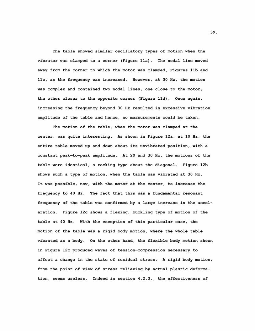
The table showed similar oscillatory types of motion when the

vibrator was clamped to a corner (Figure 11a). The nodal line moved

away from the corner to which the motor was clamped, Figures 11b and

11c, as the frequency was increased. However, at 30 Hz, the motion

was complex and contained two nodal lines, one close to the motor,

the other closer to the opposite corner (Figure 11d). Once again,

increasing the frequency beyond 30 Hz resulted in excessive vibration

amplitude of the table and hence, no measurements could be taken.

The motion of the table, when the motor was clamped at the

center, was quite interesting. As shown in Figure 12a, at 10 Hz, the

entire table moved up and down about its unvibrated position, with a

constant peak—to—peak amplitude. At 20 and 30 Hz, the motions of the

table were identical, a rocking type about the diagonal. Figure 12b

shows such a type of motion, when the table was vibrated at 30 Hz.

It was possible, now, with the motor at the center, to increase the

frequency to 40 Hz. The fact that this was a fundamental resonant

frequency of the table was confirmed by a large increase in the accel-

eration. Figure l2c shows a flexing, buckling type of motion of the

table at 40 Hz. With the exception of this particular case, the

motion of the table was a rigid body motion, where the whole table

vibrated as a body. On the other hand, the flexible body motion shown

in Figure 12c produced waves of tension—compression necessary to

affect a change in the state of residual stress. A rigid body motion,

from the point of view of stress relieving by actual plastic deforma-

tion, seems useless. Indeed in section 4.2.3., the effectiveness of

40.

flexural motion upon stress relieving has been clearly demonstrated.

Also, recently one of the manufacturers of the commercial vibratory

stress relief equipment has advised the use of a “motion sensing

transducer” which reports only the flexural motion in a workpiece.

4.2. Residual Stress Analysis

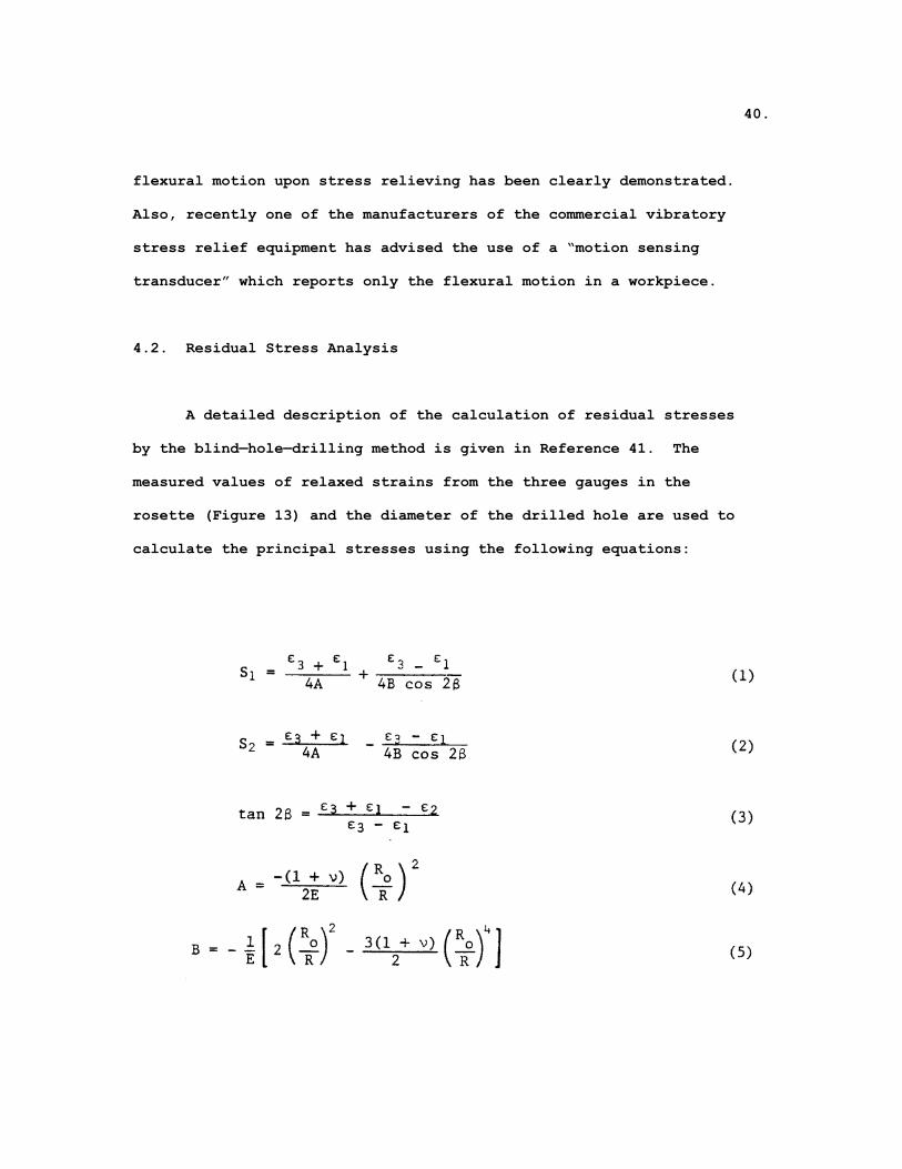
A detailed description of the calculation of residual stresses

by the blind—hole—drilling method is given in Reference 41. The

measured values of relaxed strains from the three gauges in the

rosette (Figure 13) and the diameter of the drilled hole are used to

calculate the principal stresses using the following equations:

41.

42.

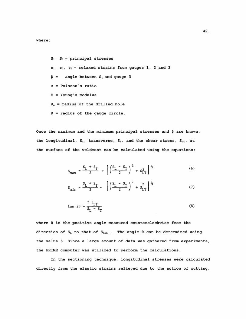
where:

S1, S2 = principal stresses

ε1, ε2, ε3 = relaxed strains from gauges 1, 2 and 3

β = angle between S1 and gauge 3

ν = Poisson’s ratio

E = Young’s modulus

Ro = radius of the drilled hole

R = radius of the gauge circle.

Once the maximum and the minimum principal stresses and β are known,

the longitudinal, SL, transverse, ST. and the shear stress, SLT, at

the surface of the weldment can be calculated using the equations:

where θ is the positive angle measured counterclockwise from the

direction of SL to that of Smin . The angle θ can be determined using

the value β. Since a large amount of data was gathered from experiments,

the PRIME computer was utilized to perform the calculations.

In the sectioning technique, longitudinal stresses were calculated

directly from the elastic strains relieved due to the action of cutting.

43.

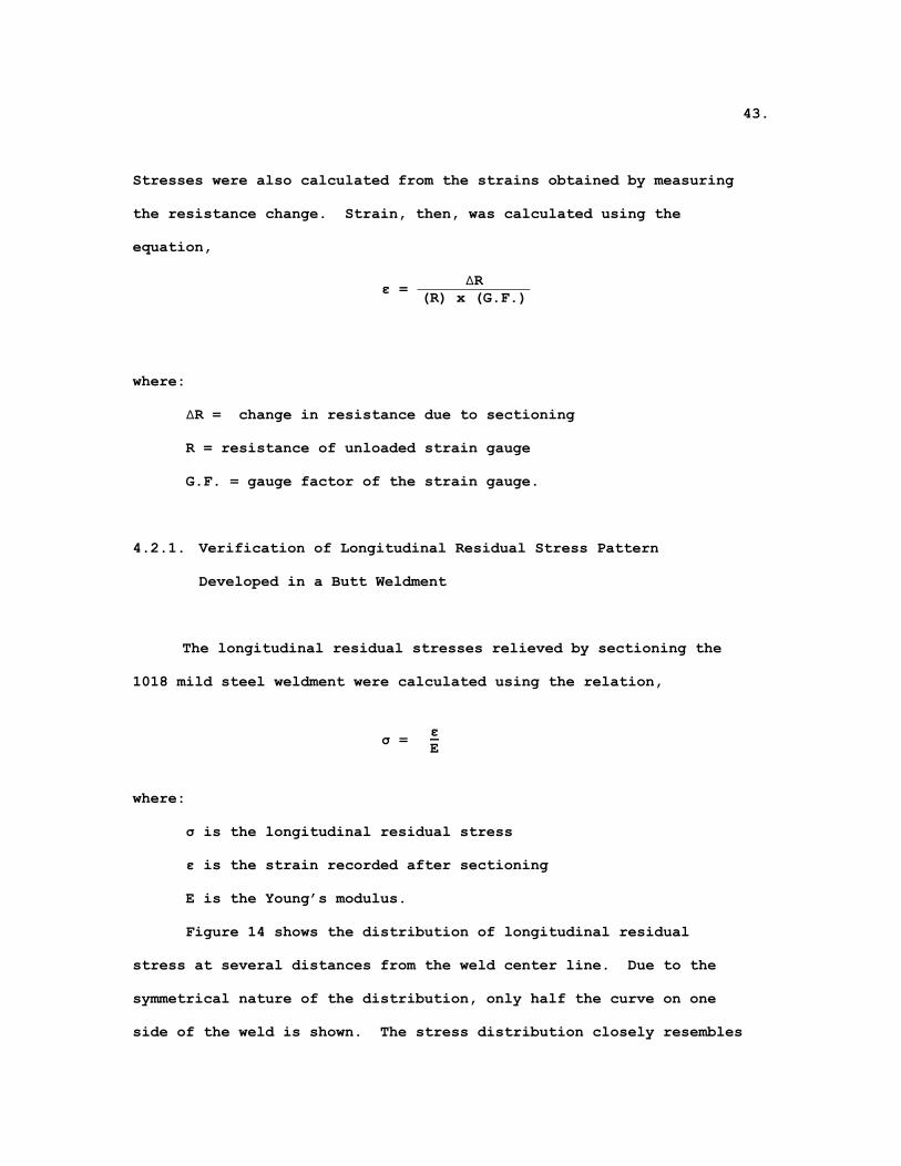
Stresses were also calculated from the strains obtained by measuring

the resistance change. Strain, then, was calculated using the

equation,

∆R ε = (R) x (G.F.)

where:

∆R = change in resistance due to sectioning

R = resistance of unloaded strain gauge

G.F. = gauge factor of the strain gauge.

4.2.1. Verification of Longitudinal Residual Stress Pattern

Developed in a Butt Weldment

The longitudinal residual stresses relieved by sectioning the

1018 mild steel weldment were calculated using the relation,

ε σ = E

where:

σ is the longitudinal residual stress

ε is the strain recorded after sectioning

E is the Young’s modulus.

Figure 14 shows the distribution of longitudinal residual

stress at several distances from the weld center line. Due to the

symmetrical nature of the distribution, only half the curve on one

side of the weld is shown. The stress distribution closely resembles

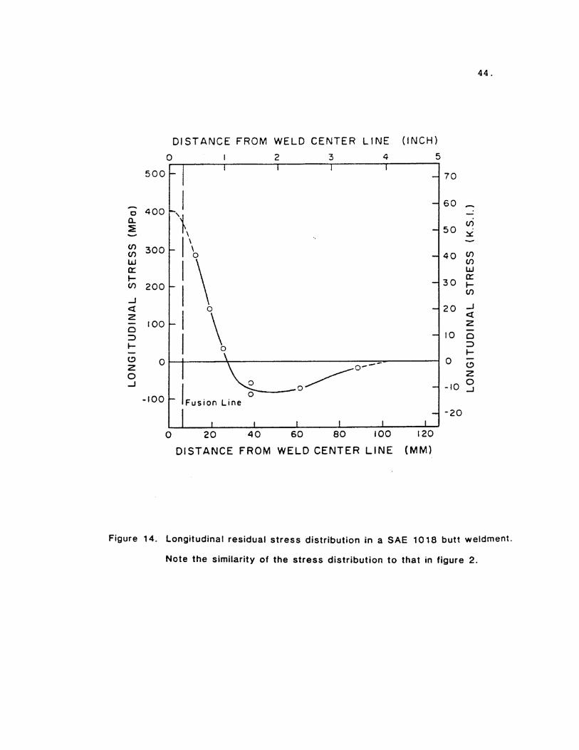
44.

45.

the general pattern of Figure 2. Also, it can be seen that the mag-

nitude of peak stresses approaches the yield point.

4.2.2. The Effect of Resonant Vibratory Treatment on the

Longitudinal Residual Stress Distribution

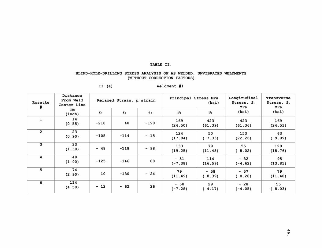
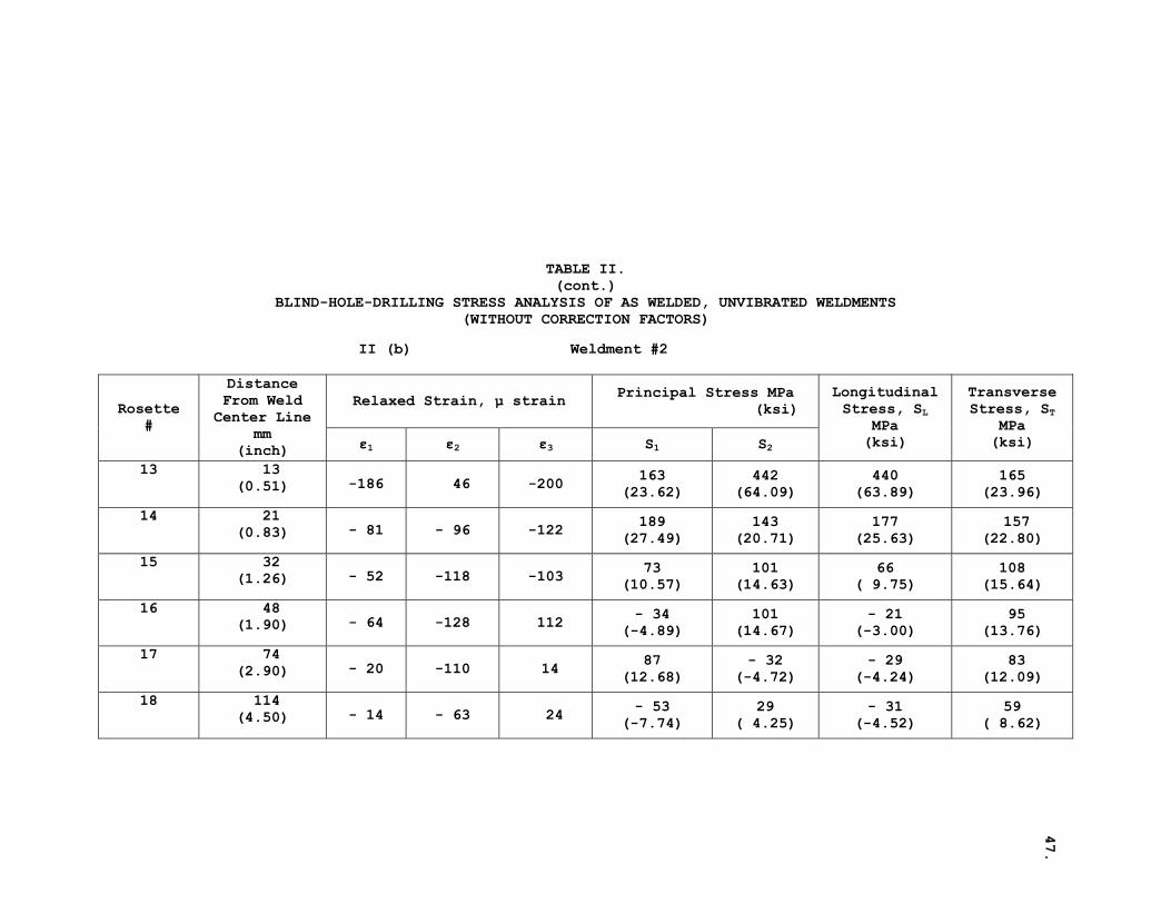
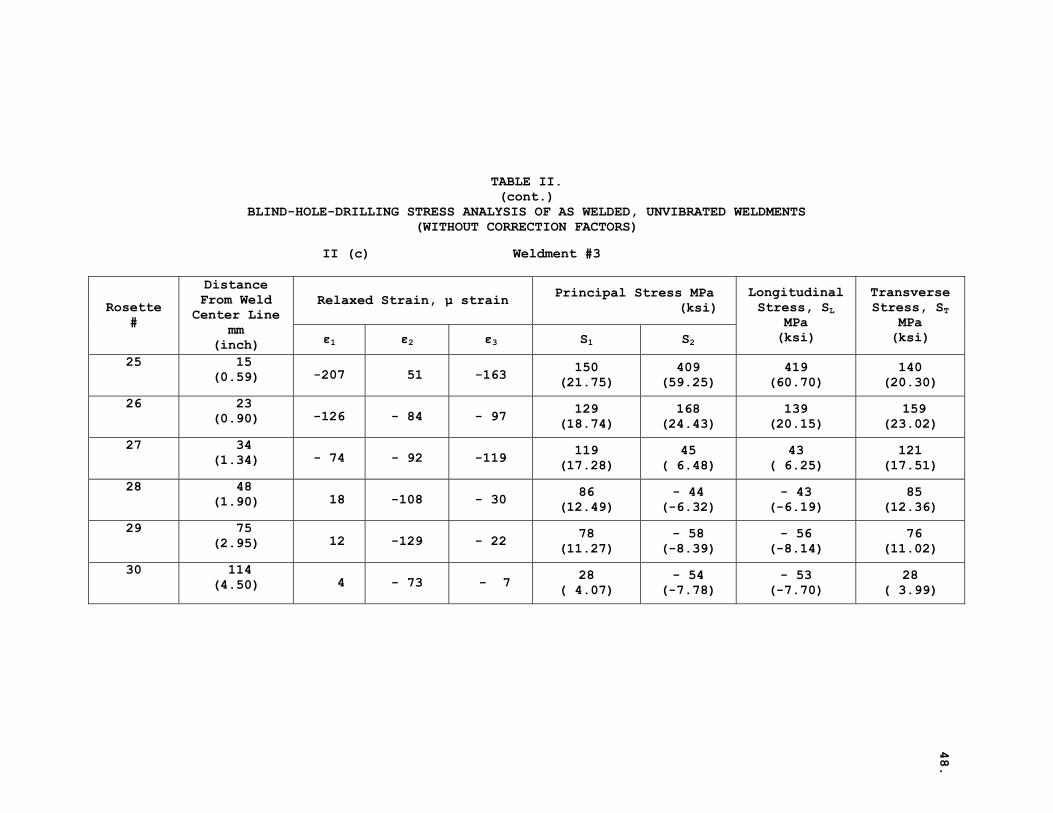
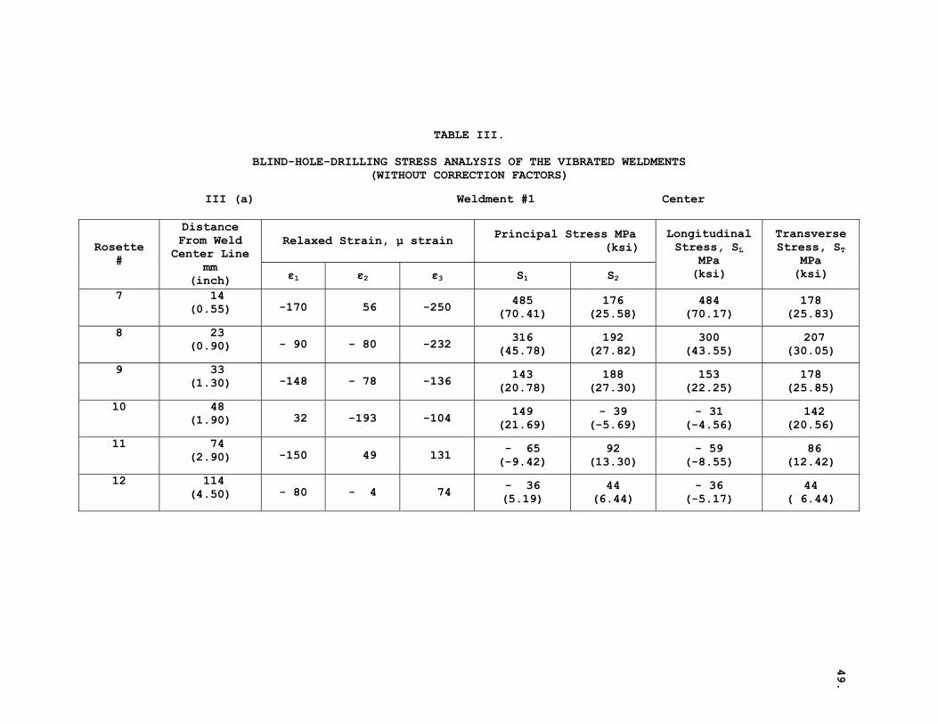
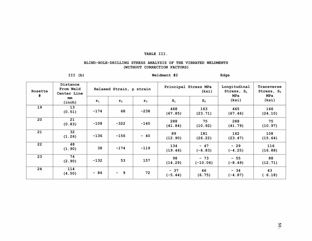
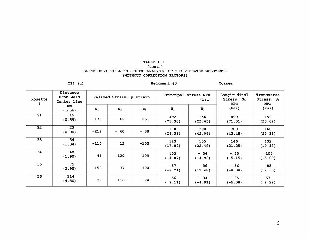
The measured relaxed strains and the calculated longitudinal

residual stresses for the three 305 x 508 x 12.7 mm weldments clamped

at different locations on the vibration table, before and after the

vibratory treatment at 40 Hz, are given in Tables II and III, respect-

ively. These strains were determined by the blind—hole—drilling

method. The average longitudinal stress distribution from the three

weldments, as a function of the distance from weld center line, is

shown graphically in Figure 15. The limitations of the blind—hole—

drilling technique when measuring stresses of the yield point magni-

tude near a weld are clearly evident from this figure. If the local

yielding effect due to the stress concentration in the vicinity of

the hole is ignored, the measured stresses can be greatly overesti-

mated.42 Measured stresses, in the base plate close to the weld,

exceeded the ultimate tensile strength indicating gross overestimation.

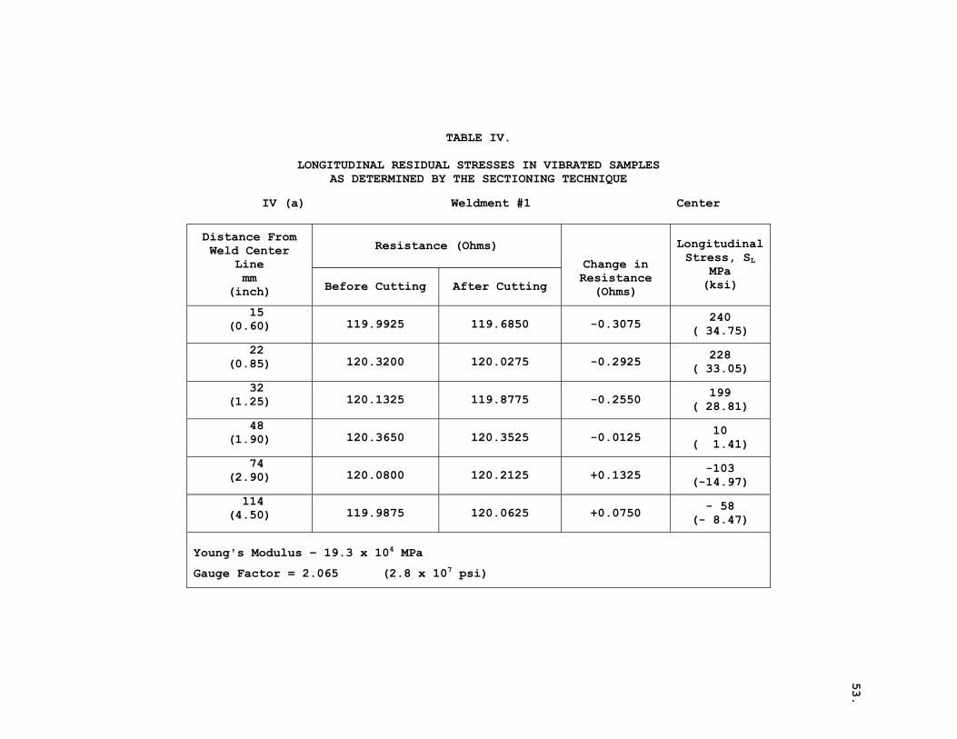
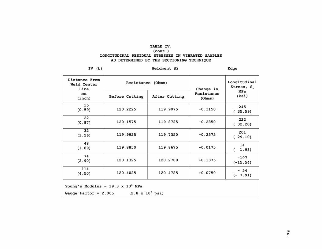
Longitudinal residual stresses after vibration were also measured by

the sectioning technique and are given in Table IV. A comparison of

the longitudinal stresses from Tables III and IV also clearly indicates

the exaggerated stresses obtained by the blind—hole—drilling tech-

nique when corrections for local plasticity effects are not made.

46.

TABLE II.

BLIND-HOLE-DRILLING STRESS ANALYSIS OF AS WELDED, UNVIBRATED WELDMENTS (WITHOUT CORRECTION FACTORS)

II (a) Weldment #1

Relaxed Strain, μ strain Principal Stress MPa (ksi) Rosette

#

Distance From Weld Center Line

mm (inch) ε1 ε2 ε3 S1 S2

Longitudinal Stress, SL

MPa (ksi)

Transverse Stress, ST

MPa (ksi)

1 14 (0.55) -218 40 -190 169

(24.50) 423

(61.39) 423

(61.36) 169

(24.53)

2 23 (0.90) -105 -114 - 15 124

(17.94) 50

( 7.33) 153

(22.26) 63

( 9.09)

3 33 (1.30) - 48 -118 - 98 133

(19.25) 79

(11.48) 55

( 8.02) 129

(18.76)

4 48 (1.90) -125 -146 80 - 51

(-7.38) 114

(16.59) - 32

(-4.62) 95

(13.81)

5 74 (2.90) 10 -130 - 24 79

(11.49) - 58

(-8.39) - 57

(-8.28) 79

(11.40)

6 114 (4.50) - 12 - 62 26 - 50

(-7.28) 29

( 4.17) - 28

(-4.05) 55

( 8.03)

47.

TABLE II. (cont.)


II (b) Weldment #2


#




MPa (ksi)


MPa (ksi)

13 13 (0.51) -186 46 -200 163

(23.62) 442

(64.09) 440

(63.89) 165

(23.96)

14 21 (0.83) - 81 - 96 -122 189

(27.49) 143

(20.71) 177

(25.63) 157

(22.80)

15 32 (1.26) - 52 -118 -103 73

(10.57) 101

(14.63) 66

( 9.75) 108

(15.64)

16 48 (1.90) - 64 -128 112 - 34

(-4.89) 101

(14.67) - 21

(-3.00) 95

(13.76)

17 74 (2.90) - 20 -110 14 87

(12.68) - 32

(-4.72) - 29

(-4.24) 83

(12.09)

18 114 (4.50) - 14 - 63 24 - 53

(-7.74) 29

( 4.25) - 31

(-4.52) 59

( 8.62)

48.

TABLE II. (cont.)


II (c) Weldment #3


#




MPa (ksi)


MPa (ksi)

25 15 (0.59) -207 51 -163 150

(21.75) 409

(59.25) 419

(60.70) 140

(20.30)

26 23 (0.90) -126 - 84 - 97 129

(18.74) 168

(24.43) 139

(20.15) 159

(23.02)

27 34 (1.34) - 74 - 92 -119 119

(17.28) 45

( 6.48) 43

( 6.25) 121

(17.51)

28 48 (1.90) 18 -108 - 30 86

(12.49) - 44

(-6.32) - 43

(-6.19) 85

(12.36)

29 75 (2.95) 12 -129 - 22 78

(11.27) - 58

(-8.39) - 56

(-8.14) 76

(11.02)

30 114 (4.50) 4 - 73 - 7 28

( 4.07) - 54

(-7.78) - 53

(-7.70) 28

( 3.99)

49.

TABLE III.

BLIND-HOLE-DRILLING STRESS ANALYSIS OF THE VIBRATED WELDMENTS (WITHOUT CORRECTION FACTORS)

III (a) Weldment #1 Center


#




MPa (ksi)


MPa (ksi)

7 14 (0.55) -170 56 -250 485

(70.41) 176

(25.58) 484

(70.17) 178

(25.83)

8 23 (0.90) - 90 - 80 -232 316

(45.78) 192

(27.82) 300

(43.55) 207

(30.05)

9 33 (1.30) -148 - 78 -136 143

(20.78) 188

(27.30) 153

(22.25) 178

(25.85)

10 48 (1.90) 32 -193 -104 149

(21.69) - 39

(-5.69) - 31

(-4.56) 142

(20.56)

11 74 (2.90) -150 49 131 - 65

(-9.42) 92

(13.30) - 59

(-8.55) 86

(12.42)

12 114 (4.50) - 80 - 4 74 - 36

(5.19) 44

(6.44) - 36

(-5.17) 44

( 6.44)

50.

TABLE III.


III (b) Weldment #2 Edge


#




MPa (ksi)


MPa (ksi)

19 13 (0.51) -174 68 -238 468

(67.85) 163

(23.71) 465

(67.46) 166

(24.10)

20 21 (0.83) -108 -322 -140 288

(41.84) 75

(10.92) 288

(41.79) 75

(10.97)

21 32 (1.26) -136 -156 - 40 89

(12.90) 181

(26.22) 162

(23.47) 108

(15.64)

22 48 (1.90) 38 -174 -119 134

(19.46) - 47

(-6.83) - 29

(-4.25) 116

(16.88)

23 74 (2.90) -132 53 157 98

(14.29) - 73

(-10.06) - 55

(-8.49) 88

(12.71)

24 114 (4.50) - 84 - 9 72 - 37

(-5.44) 46

(6.75) - 34

(-4.87) 43

( 6.18)

51.

TABLE III. (cont.)


III (c) Weldment #3 Corner


#




MPa (ksi)


MPa (ksi)

31 15 (0.59) -178 62 -261 492

(71.38) 156

(22.65) 490

(71.01) 159

(23.02)

32 23 (0.90) -212 - 60 - 88 170

(24.59) 290

(42.08) 300

(43.48) 160

(23.18)

33 34 (1.34) -115 13 -105 123

(17.89) 155

(22.48) 146

(21.25) 132

(19.13)

34 48 (1.90) 41 -129 -109 103

(14.87) - 34

(-4.93) - 35

(-5.15) 104

(15.09)

35 75 (2.95) -153 37 120 -57

(-8.21) 86

(12.48) - 56

(-8.08) 85

(12.35)

36 114 (4.50) 32 -116 - 74 56

( 8.11) - 34

(-4.91) - 35

(-5.08) 57

( 8.28)

52.

53.

TABLE IV.

LONGITUDINAL RESIDUAL STRESSES IN VIBRATED SAMPLES AS DETERMINED BY THE SECTIONING TECHNIQUE

IV (a) Weldment #1 Center

Resistance (Ohms) Distance From Weld Center

Line mm

(inch) Before Cutting After Cutting

Change in Resistance (Ohms)

LongitudinalStress, SL

MPa (ksi)

15 (0.60) 119.9925 119.6850 -0.3075 240

( 34.75)

22 (0.85) 120.3200 120.0275 -0.2925 228

( 33.05)

32 (1.25) 120.1325 119.8775 -0.2550 199

( 28.81)

48 (1.90) 120.3650 120.3525 -0.0125 10

( 1.41)

74 (2.90) 120.0800 120.2125 +0.1325 -103

(-14.97)

114 (4.50) 119.9875 120.0625 +0.0750 - 58

(- 8.47)

Young's Modulus – 19.3 x 104 MPa

Gauge Factor = 2.065 (2.8 x 107 psi)

54.

TABLE IV. (cont.)


IV (b) Weldment #2 Edge


Line mm




MPa (ksi)

15 (0.59) 120.2225 119.9075 -0.3150 245

( 35.59)

22 (0.87) 120.1575 119.8725 -0.2850 222

( 32.20)

32 (1.26) 119.9925 119.7350 -0.2575 201

( 29.10)

48 (1.89) 119.8850 119.8675 -0.0175 14

( 1.98)

74 (2.90) 120.1325 120.2700 +0.1375 -107

(-15.54)

114 (4.50) 120.4025 120.4725 +0.0750 - 54

(- 7.91)



55.

TABLE IV. (cont.)


IV (c) Weldment #3 Corner


Line mm




MPa (ksi)

15 (0.50) 119.9775 119.6650 -0.3125 243

( 35.31)

22 (0.85) 120.2425 119.9600 -0.2825 220

( 31.92)

32 (1.25) 120.0575 119.8075 -0.2500 195

( 28.25)

48 (1.90) 120.0525 120.0450 -0.0075 6

( 0.85)

74 (2.90) 120.1750 120.3000 +0.1250 - 97

(-14.12)

114 (4.50) 119.9925 120.0400 +0.0475 - 37

(- 5.37)



56.

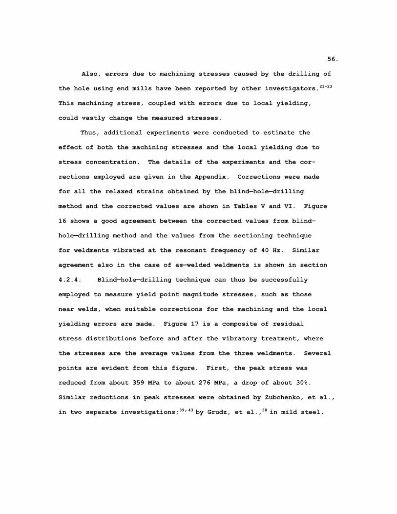
Also, errors due to machining stresses caused by the drilling of

the hole using end mills have been reported by other investigators.21-23

This machining stress, coupled with errors due to local yielding,

could vastly change the measured stresses.

Thus, additional experiments were conducted to estimate the

effect of both the machining stresses and the local yielding due to

stress concentration. The details of the experiments and the cor-

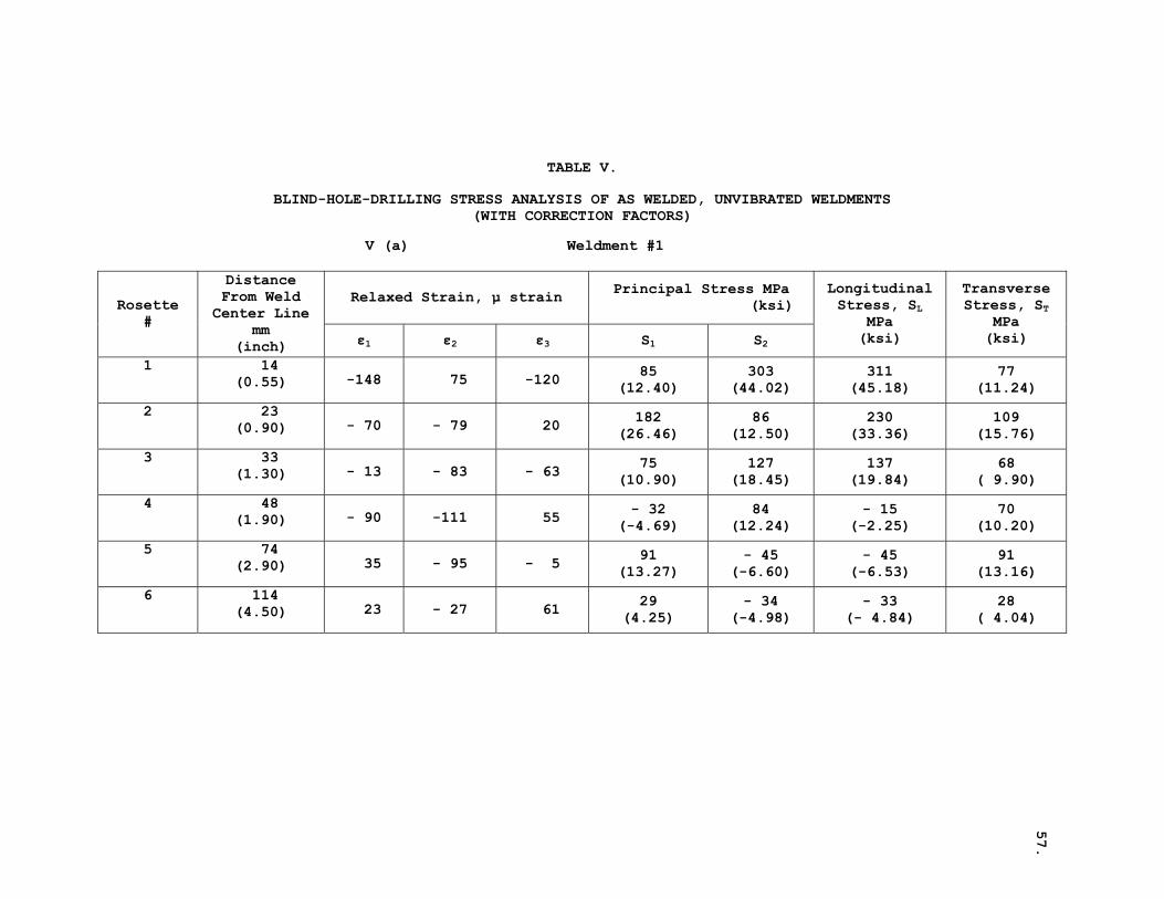
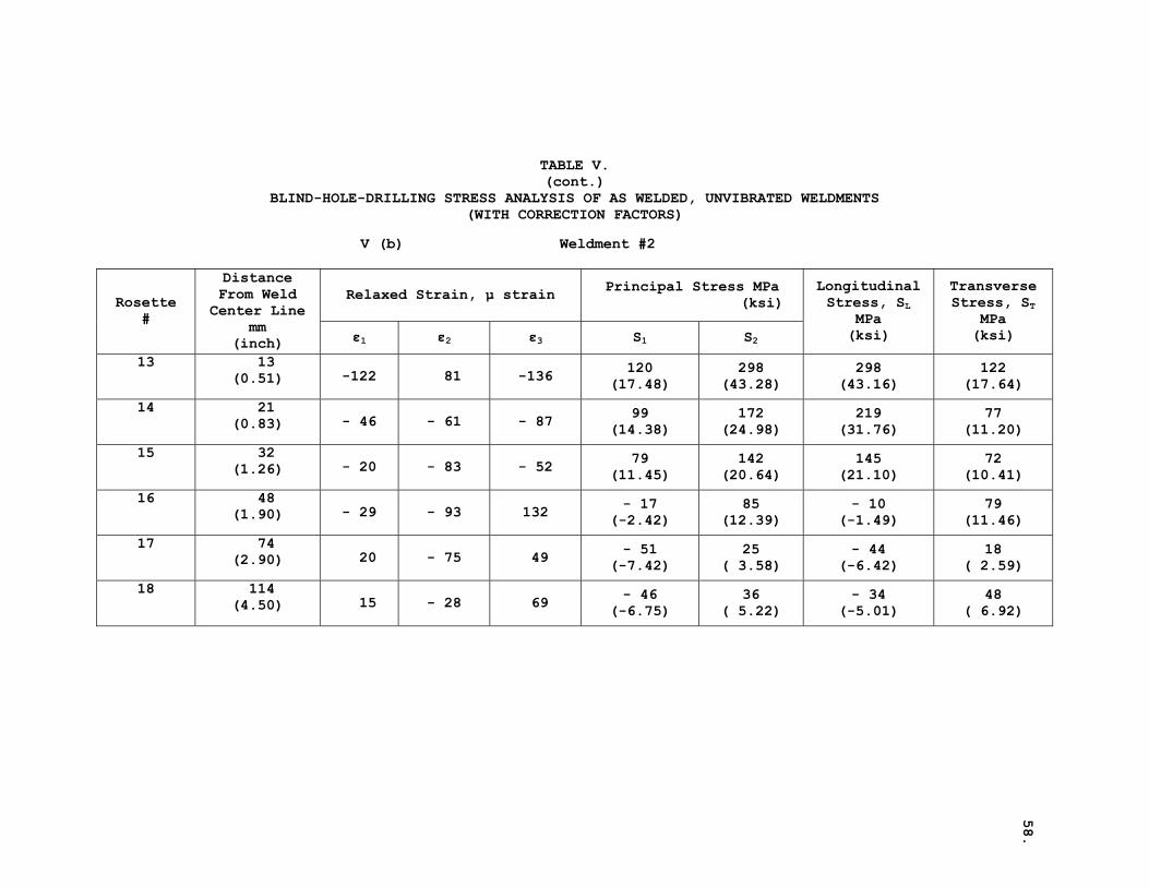
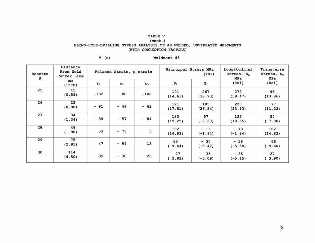
rections employed are given in the Appendix. Corrections were made

for all the relaxed strains obtained by the blind—hole—drilling

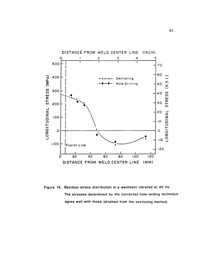
method and the corrected values are shown in Tables V and VI. Figure

16 shows a good agreement between the corrected values from blind—

hole—drilling method and the values from the sectioning technique

for weldments vibrated at the resonant frequency of 40 Hz. Similar

agreement also in the case of as—welded weldments is shown in section

4.2.4. Blind—hole—drilling technique can thus be successfully

employed to measure yield point magnitude stresses, such as those

near welds, when suitable corrections for the machining and the local

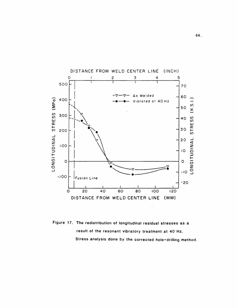
yielding errors are made. Figure 17 is a composite of residual

stress distributions before and after the vibratory treatment, where

the stresses are the average values from the three weldments. Several

points are evident from this figure. First, the peak stress was

reduced from about 359 MPa to about 276 MPa, a drop of about 30%.

Similar reductions in peak stresses were obtained by Zubchenko, et al.,

in two separate investigations;39’43 by Grudz, et al.,38 in mild steel,

57.

TABLE V.

BLIND-HOLE-DRILLING STRESS ANALYSIS OF AS WELDED, UNVIBRATED WELDMENTS (WITH CORRECTION FACTORS)

V (a) Weldment #1


#




MPa (ksi)


MPa (ksi)

1 14 (0.55) -148 75 -120 85

(12.40) 303

(44.02) 311

(45.18) 77

(11.24)

2 23 (0.90) - 70 - 79 20 182

(26.46) 86

(12.50) 230

(33.36) 109

(15.76)

3 33 (1.30) - 13 - 83 - 63 75

(10.90) 127

(18.45) 137

(19.84) 68

( 9.90)

4 48 (1.90) - 90 -111 55 - 32

(-4.69) 84

(12.24) - 15

(-2.25) 70

(10.20)

5 74 (2.90) 35 - 95 - 5 91

(13.27) - 45

(-6.60) - 45

(-6.53) 91

(13.16)

6 114 (4.50) 23 - 27 61 29

(4.25) - 34

(-4.98) - 33

(- 4.84) 28

( 4.04)

58.

TABLE V. (cont.)


V (b) Weldment #2


#




MPa (ksi)


MPa (ksi)

13 13 (0.51) -122 81 -136 120

(17.48) 298

(43.28) 298

(43.16) 122

(17.64)

14 21 (0.83) - 46 - 61 - 87 99

(14.38) 172

(24.98) 219

(31.76) 77

(11.20)

15 32 (1.26) - 20 - 83 - 52 79

(11.45) 142

(20.64) 145

(21.10) 72

(10.41)

16 48 (1.90) - 29 - 93 132 - 17

(-2.42) 85

(12.39) - 10

(-1.49) 79

(11.46)

17 74 (2.90) 20 - 75 49 - 51

(-7.42) 25

( 3.58) - 44

(-6.42) 18

( 2.59)

18 114 (4.50) 15 - 28 69 - 46

(-6.75) 36

( 5.22) - 34

(-5.01) 48

( 6.92)

59.

TABLE V. (cont.)


V (c) Weldment #3


#




MPa (ksi)


MPa (ksi)

25 15 (0.59) -132 80 -108 101

(14.63) 267

(38.70) 272

(39.47) 96

(13.86)

26 23 (0.90) - 91 - 49 - 62 121

(17.51) 185

(26.84) 228

(33.13) 77

(11.23)

27 34 (1.34) - 39 - 57 - 84 133

(19.25) 57

( 8.20) 135

(19.55) 54

( 7.90)

28 48 (1.90) 53 - 73 5 102

(14.83) - 13

(-1.94) - 13

(-1.94) 102

(14.83)

29 75 (2.95) 47 - 94 13 65

( 9.44) - 37

(-5.42) - 38

(-5.58) 66

( 9.60)

30 114 (4.50) 39 - 38 28 27

( 3.82) - 35

(-5.09) - 35

(-5.15) 27

( 3.90)

60.

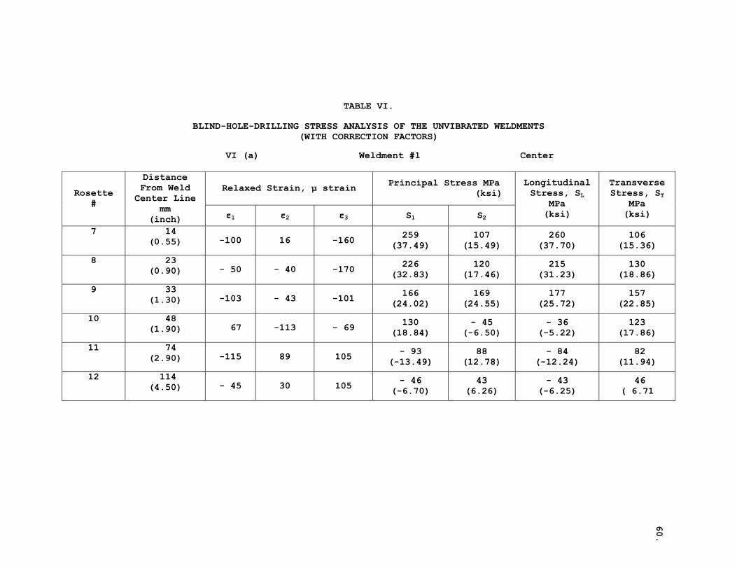
TABLE VI.

BLIND-HOLE-DRILLING STRESS ANALYSIS OF THE UNVIBRATED WELDMENTS (WITH CORRECTION FACTORS)

VI (a) Weldment #1 Center


#




MPa (ksi)


MPa (ksi)

7 14 (0.55) -100 16 -160 259

(37.49) 107

(15.49) 260

(37.70) 106

(15.36)

8 23 (0.90) - 50 - 40 -170 226

(32.83) 120

(17.46) 215

(31.23) 130

(18.86)

9 33 (1.30) -103 - 43 -101 166

(24.02) 169

(24.55) 177

(25.72) 157

(22.85)

10 48 (1.90) 67 -113 - 69 130

(18.84) - 45

(-6.50) - 36

(-5.22) 123

(17.86)

11 74 (2.90) -115 89 105 - 93

(-13.49) 88

(12.78) - 84

(-12.24) 82

(11.94)

12 114 (4.50) - 45 30 105 - 46

(-6.70) 43

(6.26) - 43

(-6.25) 46

( 6.71

61.

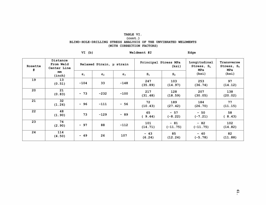
TABLE VI. (cont.)


VI (b) Weldment #2 Edge


#




MPa (ksi)


MPa (ksi)

19 13 (0.51) -104 33 -148 247

(35.89) 103

(14.97) 253

(36.74) 97

(14.12)

20 21 (0.83) - 73 -232 -100 217

(31.48) 128

(18.59) 207

(30.05) 138

(20.02)

21 32 (1.26) - 96 -111 - 56 72

(10.43) 189

(27.42) 184

(26.70) 77

(11.15)

22 48 (1.90) 73 -129 - 89 65

( 9.44) - 57

(-8.22) - 50

(-7.21) 58

( 8.43)

23 74 (2.90) - 97 88 -112 101

(14.71) - 81

(-11.75) - 82

(-11.75) 102

(14.82)

24 114 (4.50) - 49 26 107 - 43

(6.24) 85

(12.24) - 40

(-5.78) 82

(11.88)

62.

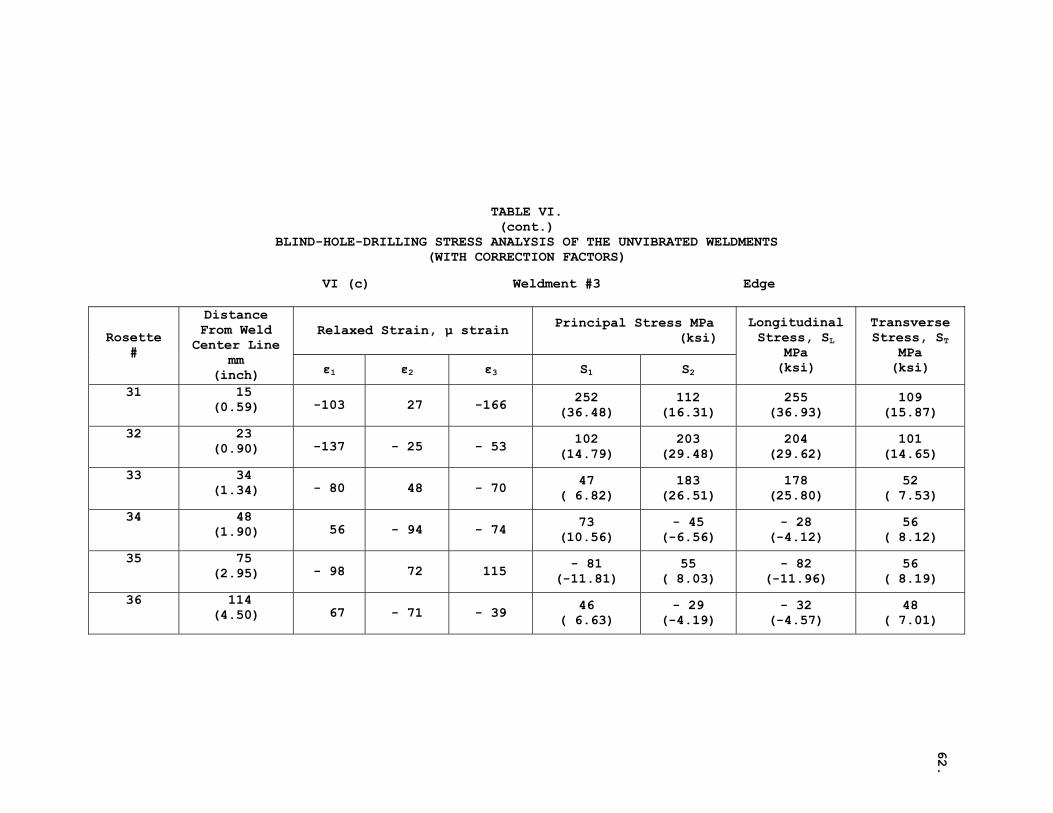
TABLE VI. (cont.)


VI (c) Weldment #3 Edge


#




MPa (ksi)


MPa (ksi)

31 15 (0.59) -103 27 -166 252

(36.48) 112

(16.31) 255

(36.93) 109

(15.87)

32 23 (0.90) -137 - 25 - 53 102

(14.79) 203

(29.48) 204

(29.62) 101

(14.65)

33 34 (1.34) - 80 48 - 70 47

( 6.82) 183

(26.51) 178

(25.80) 52

( 7.53)

34 48 (1.90) 56 - 94 - 74 73

(10.56) - 45

(-6.56) - 28

(-4.12) 56

( 8.12)

35 75 (2.95) - 98 72 115 - 81

(-11.81) 55

( 8.03) - 82

(-11.96) 56

( 8.19)

36 114 (4.50) 67 - 71 - 39 46

( 6.63) - 29

(-4.19) - 32

(-4.57) 48

( 7.01)

63.

64.

65.

aluminum and titanium alloy weldments; and by Weiss, et al.,40 in a

plain carbon steel weldment.

Second, the residual stresses were not completely eliminated by

the vibratory treatment, although several Russian authors have

noticed up to 90% reduction in residual stresses.44 On the other

hand, there seemed to be a redistribution of residual stresses across

the weld. A similar stress redistribution has been noticed by other

investigators. 38,39

Thus, resonant vibratory treatment when applied to mild steel

weldments resulted in a definite redistribution of longitudinal

stresses, and reduction in the peak residual stresses very close to

the weld. The actual mechanism by which the stress reduction occurred

will be discussed in section 4.3.

4.2.3. Effectiveness of the Vibratory Treatment on the Location

of Weldments

An examination of the longitudinal residual stress values from

Table VI shows that due to the resonant vibratory treatment, all the

three weldments have achieved about the same residual stress distri-

bution, regardless of their position on the table during vibration.

The considerable bending moments and torques noticed on the table at

resonant frequency seem to act along a passing wave rather than a

stationary wave. This would naturally expose any location on the

table to the same amount of bending moment and thus make all the

locations on the vibration table equally effective for the treatment.

66.

The effectiveness of the treatment, within the length of each

weldment, too, seems uniform. In a 305 mm long weld, the longitud-

inal stresses would remain constant in a region at the center and

begin to decrease toward the ends. Conservatively, the middle 150 mm

long portion of the weld can be assumed to have uniform stresses,

with stresses decreasing in 75 mm regions on either end. In the

residual stress measurement, holes were randomly drilled in a 100 mm

long region at the center of each weldment. For example, in one

weldment holes closest to the weld were drilled in the middle of

the weldment, while in the other two, the holes were drilled 50 mm

on either side of the center of the weld. Similarly, other holes

were drilled on a random basis. Despite the randomness in the loca-

tion of the holes, there was uniformity of stress redistribution in

all three weldments, at least in the central 100 mm region.

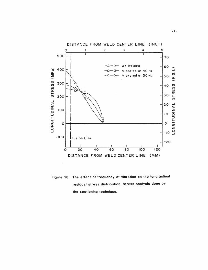
4.2.4. The Effect of Frequency of Vibration on the Longitudinal

Residual Stress Distribution

The three 914 x 406 x 12.7 mm butt weldments were used in the

study of the role of frequency of vibration on the residual stress

distribution in the weldments. One weldment was given the standard

resonance treatment at 40 Hz; the second, a sub—resonance treatemnt

at 30 Hz; and the third was not vibrated and was used as a control.

It was decided to monitor the stresses in the weldments using x—ray

and sectioning techniques of stress measurement. For the purpose of

x—ray studies, it was necessary to cut out a 127 mm square piece from

67.

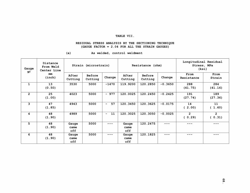
the middle of each weldment. Stresses relieved due to this section-

ing were monitored and are given in Table VII for the three weldments

studied. It was assumed that sectioning the 127 mm square pieces

would not significantly relieve the stresses and that most of the

residual stresses would be still locked up in those pieces. However,

as seen in Table VII, and from the residual stress distributions

plotted in Figure 18, it appeared that sectioning has relieved the

majority of the locked—in stresses and that insignificant amounts of

stress would be left in the 127 mm square pieces. Even though the

x—ray analysis showed stresses of the order of 7 to 55 MPa in some

locations, these stress values were not added onto those obtained

from the sectioning method because of the inherently low accuracy of

stress measurement (about 35 MPa) by this method due to the large

grain size involved in the samples. Further, the stress readings

were so randomly distributed without any trend of the classic stress

distribution of Figure 2, it was assumed that sectioning had prac-

tically relieved all the residual stresses.

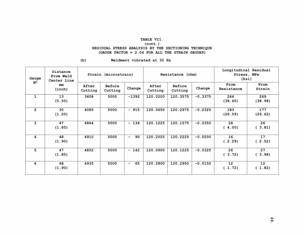
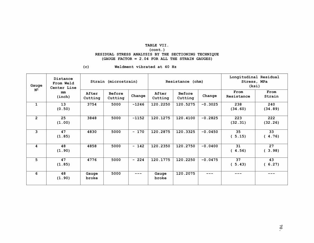
Referring to Figure 18, once again there was substantial reduc-

tion in peak stresses (from about 380 MPa to about 250 MPa) due to

the resonance treatment at 40 Hz, coupled with stress redistribution

similar in nature to that shown in Figure 17. For the 305 x 508 x

12.7 mm weldments, though there was a general stress reduction due

to the sub—resonance treatment at 30 Hz, vibrating at resonant

frequency apparently was more effective than that at a sub—resonant

frequency.

68.

TABLE VII.

RESIDUAL STRESS ANALYSIS BY THE SECTIONING TECHNIQUE (GAUGE FACTOR = 2.04 FOR ALL THE STRAIN GAUGES)

(a) As welded, control weldment

Strain (microstrain) Resistance (ohm) Longitudinal Residual

Stress, MPa (ksi) Gauge

No


mm (inch)

After Cutting

Before Cutting Change After

Cutting Before Cutting Change

From Resistance

From Strain

1 13 (0.50)

3530 5000 -1470 119.9200 120.2850 -0.3650 288 (41.75)

284 (41.16)

2 25 (1.00)

4023 5000 - 977 120.0025 120.2450 -0.2425 191 (27.74)

189 (27.36)

3 47 (1.85)

4943 5000 - 57 120.3450 120.3625 -0.0175 14 ( 2.00)

11 ( 1.60)

4 48 (1.90)

4989 5000 - 11 120.3025 120.3050 -0.0025 2 ( 0.29)

2 ( 0.31)

5 48 (1.90)

Gauge came off

5000 --- Gauge came off

120.2475 --- --- ---

6 48 (1.90)

Gauge came off

5000 --- Gauge came off

120.1825 --- --- ---

69.

TABLE VII. (cont.)


(b) Weldment vibrated at 30 Hz



No


mm (inch)

After Cutting



From Resistance

From Strain

1 13 (0.50)

3608 5000 -1392 120.0200 120.3575 -0.3375 266 (38.60)

269 (38.98)

2 30 (1.20)

4085 5000 - 915 120.0650 120.2975 -0.2325 183 (26.59)

177 (26.62)

3 47 (1.85)

4864 5000 - 136 120.1225 120.1575 -0.0350 28 ( 4.00)

26 ( 3.81)

4 48 (1.90)

4910 5000 - 90 120.2025 120.2225 -0.0200 16 ( 2.29)

17 ( 2.52)

5 47 (1.85)

4852 5000 - 142 120.0900 120.1225 -0.0325 26 ( 3.72)

27 ( 3.98)

6 48 (1.90)

4935 5000 - 65 120.2800 120.2950 -0.0150 12 ( 1.72)

12 ( 1.82)

70.

TABLE VII. (cont.)


(c) Weldment vibrated at 40 Hz



No


mm (inch)

After Cutting



From Resistance

From Strain

1 13 (0.50)

3754 5000 -1246 120.2250 120.5275 -0.3025 238 (34.60)

240 (34.89)

2 25 (1.00)

3848 5000 -1152 120.1275 120.4100 -0.2825 223 (32.31)

222 (32.26)

3 47 (1.85)

4830 5000 - 170 120.2875 120.3325 -0.0450 35 ( 5.15)

33 ( 4.76)

4 48 (1.90)

4858 5000 - 142 120.2350 120.2750 -0.0400 31 ( 4.56)

27 ( 3.98)

5 47 (1.85)

4776 5000 - 224 120.1775 120.2250 -0.0475 37 ( 5.43)

43 ( 6.27)

6 48 (1.90)

Gauge broke

5000 --- Gauge broke

120.2075 --- --- ---

71.

72. As shown in Figure 19, in the case of an as—welded unvibrated

weldment, the agreement between the corrected hole—drilling stress

values obtained from the three 305 x 508 x 12.7 mm weldments and from

the 914 x 406 x 12.7 mm control weldment was excellent. Once again,

this proved that the corrected hole—drilling technique was comparable

in accuracy to that of the sectioning method. Figure 20 shows the

residual stress distribution for the four weldments vibrated at 40 Hz,

indicating definite overall stress redistribution due to the vibratory

treatment, whether the stress was measured by the sectioning or by the

blind—hole—drilling technique.

4.2.5. Effect on Macrostresses

It has been shown in a number of investigations36-40 that actual

stress reduction occurs during vibrational treatments only in those

locations where the combined residual vibratory stresses exceeded

the yield point of the material. Usually these locations were where

high stress concentration occurs, like the region adjacent to a weld.

However, if the entire part being vibrated had a uniform stress level,

a level close to the yield point of the material, will the vibratory

treatment reduce the stress level? In order to test the action of

vibratory treatment on high, uniform macrostresses, the tension weld—

ment shown in Figure 4 was vibrated at its resonance. Table VIII shows

the stress values obtained at three locations by the corrected hole

drilling method. It can be seen that the plate developed an average

residual tensile stress of about 234 MPa in a direction parallel to

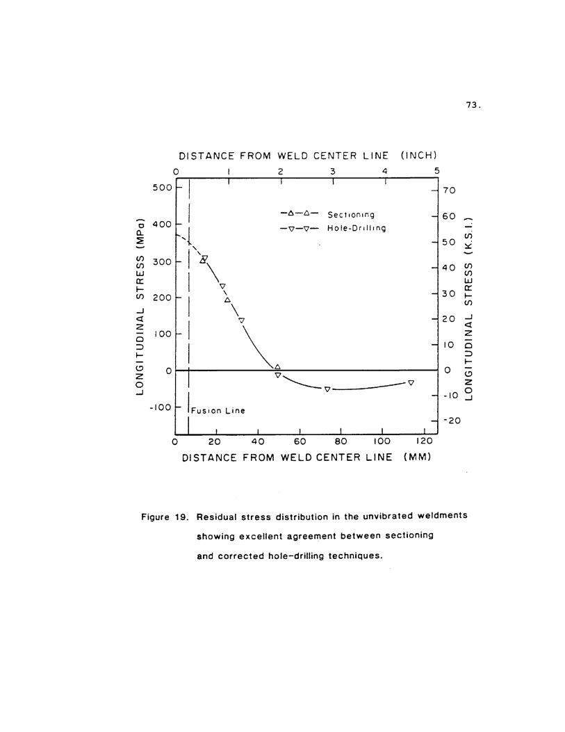
73.

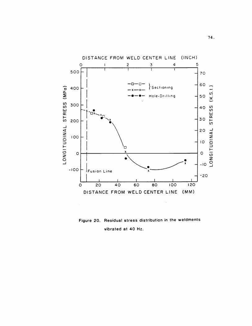
74.

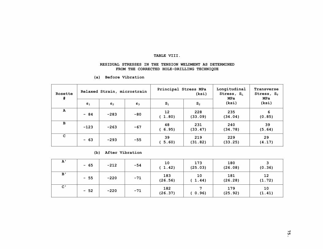
75.

TABLE VIII.

RESIDUAL STRESSES IN THE TENSION WELDMENT AS DETERMINED FROM THE CORRECTED HOLE-DRILLING TECHNIQUE

(a) Before Vibration

Relaxed Strain, microstrain Principal Stress MPa (ksi) Rosette

# ε1 ε2 ε3 S1 S2


MPa (ksi)


MPa (ksi)

A - 84 -283 -80 12

( 1.80) 228

(33.09) 235

(34.04) 6

(0.85)

B -123 -263 -67 48

( 6.95) 231

(33.47) 240

(34.78) 39

(5.64)

C - 63 -293 -55 39

( 5.60) 219

(31.82) 229

(33.25) 29

(4.17)

(b) After Vibration

A' - 65 -212 -54 10

( 1.42) 173

(25.03) 180

(26.08) 3

(0.36)

B' - 55 -220 -71 183

(26.56) 10

( 1.44) 181

(26.28) 12

(1.72)

C' - 52 -220 -71 182

(26.37) 7

( 0.96) 179

(25.92) 10

(1.41)

76.

its length. The stresses measured using a mechanical extensometer

also were approximately the same. There was virtually no transverse

stress developed in the plate. On vibrating at a resonant frequency

of 37 Hz for 20 minutes, the average residual tensile stress dropped

to about 179 MPa.

4.3. Microstructural Analysis

Although it has been often proposed by a number of investiga—

tors37~° that peak residual stresses are reduced when combined

residual and vibratory stresses exceed the yield point of the mater-

ial, there are no direct observations of the evidence of the attendant

plastic deformation. This is surprising, considering the interest in

the industrial usage of vibratory stress relief techniques. To date,

only Prohaszka, et al.,45 explained their observed stress relief due

to vibration by the dislocation theory. However, even they have not

reported direct microscopic examination of the dislocation behavior

they proposed.

In this investigation transmission electron microscopic analysis

was done to observe the dislocation nature in both annealed and in

vibrated samples. Due to the complex nature of microstructure next

to a weld, the observation and interpretation of dislocation struc-

tures were extremely difficult. However, due to the observed reduc-

tion of the stresses in the A—36 tension plate weldment, samples for

microscopic examination were obtained from the tension plate. Since

the plate was in an annealed condition, before introducing tensile

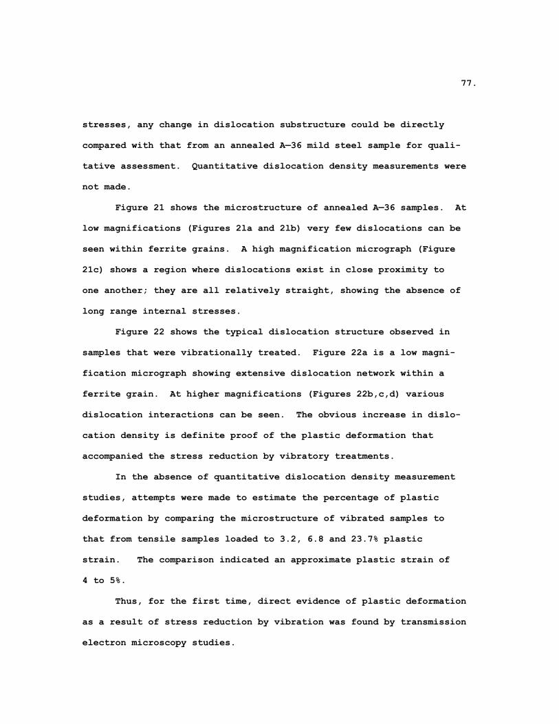
77.

stresses, any change in dislocation substructure could be directly

compared with that from an annealed A—36 mild steel sample for quali-

tative assessment. Quantitative dislocation density measurements were

not made.

Figure 21 shows the microstructure of annealed A—36 samples. At

low magnifications (Figures 2la and 2lb) very few dislocations can be

seen within ferrite grains. A high magnification micrograph (Figure

21c) shows a region where dislocations exist in close proximity to

one another; they are all relatively straight, showing the absence of

long range internal stresses.

Figure 22 shows the typical dislocation structure observed in

samples that were vibrationally treated. Figure 22a is a low magni-

fication micrograph showing extensive dislocation network within a

ferrite grain. At higher magnifications (Figures 22b,c,d) various

dislocation interactions can be seen. The obvious increase in dislo-

cation density is definite proof of the plastic deformation that

accompanied the stress reduction by vibratory treatments.

In the absence of quantitative dislocation density measurement

studies, attempts were made to estimate the percentage of plastic

deformation by comparing the microstructure of vibrated samples to

that from tensile samples loaded to 3.2, 6.8 and 23.7% plastic

strain. The comparison indicated an approximate plastic strain of

4 to 5%.

Thus, for the first time, direct evidence of plastic deformation

as a result of stress reduction by vibration was found by transmission

electron microscopy studies.

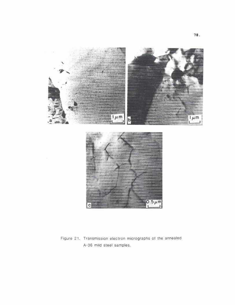
78.

79.

80.

4.4 Effect on Mechanical Properties

One of the main concerns of the usage of vibratory techniques of

stress relief is potential fatigue damage.37 In most instances,

fatigue failure is due to already—present cracks which open up upon

vibrating32. In actual practice, there are very few reports of damage

of vibrated parts due to fatigue failure.

In order to test the effect of vibration on fatigue properties

in the case of welds that showed pronounced stress redistribution,

fatigue tests were conducted using samples obtained from the three

914 x 406 x 12.7 mm weldments. Figures 23, 24 and 25 shown the S—N

curves for the samples from control weldment, weldment vibrated at

30 Hz and at 40 Hz respectively. Tensile testing was also performed

on these weldments and the summary of results is shown in Table 9.

The fatigue limit did not change as a result of either the sub—

resonance or the resonance treatment. The tensile stress remained

the same. However, there was a slight increase in the yield strength

of about 38 MPa as a result of the resonance treatment. This result

is consistent with the observation of plastic deformation, which

could lead to work hardening and hence, an increase in yield strength.

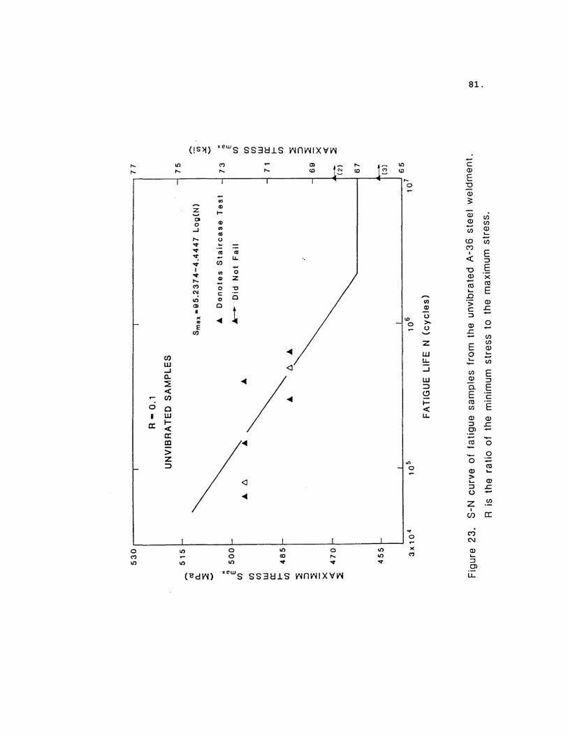
81.

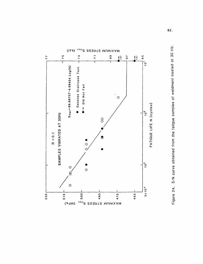
82.

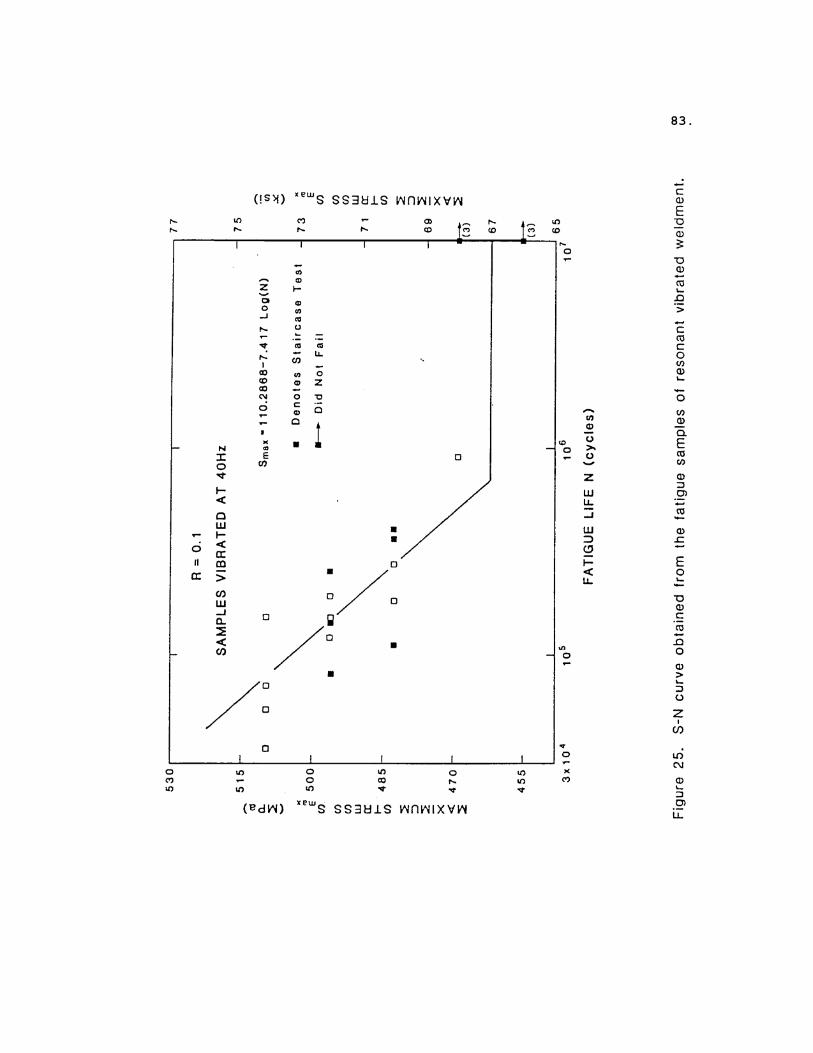
83.

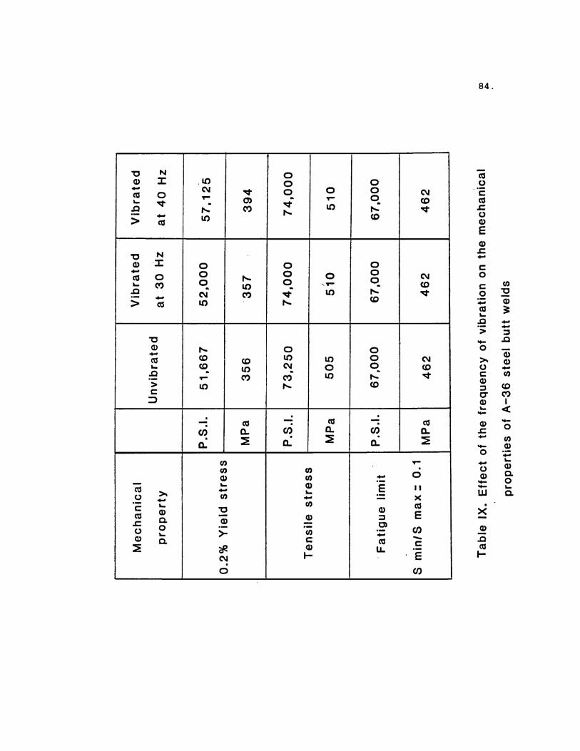
84.

85.

CHAPTER 5

CONCLUSIONS

The following conclusions were drawn from this investigation:

1. Vibratory stress relief treatment performed at the resonant

frequency effectively redistributed the residual stresses in A—36 butt

weldments.

2. The sub—resonance treatment apparently was less effective

than the treatment at the resonant frequency.

3. When a vibration table is used to treat smaller samples, the

effectiveness of the treatment was the same irrespective of the

location of the sample.

4. As a result of the treatments, a reduction of about 30% was

noticed in peak longitudinal residual stresses in A—36 butt weldments.

5. Unlike some of the thermal treatments, residual stresses did

not vanish as a result of the vibratory treatment.

6. Transmission electron microscopy studies indicated that the

mechanism by which peak—stress reduction occurs is one of plastic

deformation.

7. There was no fatigue damage as a result of the vibratory

treatment.

8. The tensile properties of the weldment did not change as a

result of the treatment.

86.

9. Hole—drilling techniques can be effectively used to measure

yield point level stresses by taking into account the machining strains

and the strains due to local yielding as a result of stress concentra-

tion.

10. The accuracy of the corrected hole—drilling technique

approached that of a sectioning method.

87.

REFERENCES

1. “Vibratory Stress Relief”, Weld. Eng., 1967, vol. 52, p. 46. 2. “Big Shake Takes the Stress out of Metal”, Chem. Week, 1967, vol.

101, p. 119. 3. R. A. Claxton: Heat Treat. Met., 1974, vol. 1, p. 131. 4. J. Varga: FWP J., 1974, vol. 14, p. 23. 5. G. G. Saunders and R. A. Claxton: Proc. Int. Conf. on Residual

Stresses in Welded Construction and their Effects, London,England, vol. 1, p. 173, 1977.

6. K. C. Schofield: Int. J. Pressure Vessels Piping, 1976, vol. 4,

p. 1. 7. A. A. Denton: Metall. Rev., 1966, vol. 11, p. 1. 8. R. P. Frick, G. A. Gurtman, and H. D. Meriwether: J. Mater.,1967,

vol. 2, p. 719. 9. C. S. Barrett: Proc. Soc. Exp. Stress Anal., 1944, vol. 2, p.147. 10. B. D. Cullity: Elements of X—Ray Diffraction, p. 431, Addison—

Wesley Publ. Co., Reading, MA, 1956. 11. H. P. Klug and L. E. Alexander: X—Ray Diffraction Procedures, p.

755, John Wiley and Sons, Inc., New York, 1974. 12. “Residual Stress Measurement by X—Ray Diffraction—--SAE J 784a”,

2nd Edition, Society of Automotive Engineers, Inc., 1971. 13. J.B. Cohen, M. R. James and B. A. MacDonald: Nav. Res. Rev.,1978,

vol. 31, p. 1. 14. J. Mathar: Trans. ASME, 1934, vol. 54, p. 249. 15. W. Soete and R. Vancrombrugge: Proc. Soc. Exp. Stress Anal.,1950,

vol. 8, p. 17. 16. E. W. Suppiger, C. Riparbelli and E. R. Ward: Weld J., 1951, vol.

30, p. 91—s. 17. N. J. Rendler and I. Vigness: Exp. Mech., 1966, vol. 6, p. 577.

88.

18. R. A. Kelsey: Proc. Soc. Exp. Stress Anal., 1956, vol. 14, P. 181.

19. S. P. Timoshenko and J. N. Goodier: Theory of Elasticity, 3rd

Edition, p. 71, McGraw—Hill, New York, 1970. 20. R. G. Bathgate: Strain, 1968, vol. 4, p. 20. 21. A. J. Bush and F. J. Kromer: ISA Trans., 1973, vol. 12, p. 249. 22. E. M. Beaney and E. Procter: Strain, 1974, vol. 10, p. 7. 23. S. S. Birley and A. Owens: NDT mt., 1980, vol. 13, p. 3. 24. E. N. Beaney: Strain, 1976, vol. 12, p. 99. 25. D. Rosenthal: Weld. J., 1941, vol. 20, p. 220—s. 26. Rodgers and Fetcher: Weld. J., 1938, vol. 17, p. 4—s. 27. K. Masubuchi: Weld. .3., 1960, vol. 39, p. 525—s. 28. L. Tall: Weld. .3., 1964, vol. 43, p. 10—s. 29. A. G. Kamtekar, J. D. White and J. B. Dwight: J. Strain Anal.

Eng. Des., 1977, vol. 12, p. 140. 30. C. J. Merrick and U. A. Schneider: Proc. Int. Conf. on Control of

Distortion and Residual Stress in Weldments, sponsored by Am. Soc. Metals, Chicago, Ill., p. 62, 1976.

31. “Stress Relieve Big Weldments in Minutes with Vibration”, Machinery,

1968, vol. 74, p. 100. 32. “A Vibration Shakedown”, Weld. Des. Fabr., 1969, vol. 42, p. 81. 33. T. D. Kelso: Tool Manuf. Eng., 1968, vol. 3, p. 48. 34. “Vibratory Stress—Relieving”, Weld. Met. Fabr., 1968, vol. 36, p.

212. 35. D. S. Keller: “Ultrasonic Stress Relieving”, Met. Treat. (Rocky

Mount N.C.), 1970, vol. 21, p. 14. 36. S. R. Rich: Weld. Eng., 1969, vol. 54, p. 44. 37. G. P. Wozney and G. R. Crawmer: Weld. J., 1968, vol. 48,p. 411—s.

89. 38. A. A. Grudz, et al.: Autom. Weld. Engl. Transi., 1972, vol. 25,

p. 70. 39. O. I. Zubchenko, A. A. Grudz, G. T. Orekhov and A. G. Sostin:

Autom. Weld. Engl. Transl., 1974, vol. 27, P. 59. 40. S. Weiss, G. S. Baker and R. D. Das Gupta: Weld. J., 1976, vol.

56, p. 47—s. 41. C. M. Tran: M. S. Dissertation, Portland State University, Port-

land, OR, 1977. 42. A. M. Nawwar, K. McLachlan and J. Shewchuk: Exp. Mech., 1976,

vol. 16, p. 226. 43. 0. I. Zubchenko, et al.: Autom. Weld. Engl. Transl., 1976, vol.

29, p. 53. 44. A. Ya. Nedoseka, et al.: Autom. Weld. Engl. Transl., 1974, vol.

27, p. 61. 45. J. Prohaszka, B. Hidasi and L. Varga: Period. Polytech. Mech. Eng.,

1975, vol. 19, p. 69. 46. I. G. Polotskii, et al.,: Autom. Weld. Engl. Transl., 1974, vol.

27, p. 67. 47. A. Puskar: Acta Met., 1976, vol. 24, p. 861.

90.

APPENDIX

91.

CORRECTIONS FOR BLIND—HOLE—DRILLING ANALYSIS

Since the hole—drilling technique of residual stress measurement

was employed to monitor the stress distribution near a weld, where the

stresses (especially longitudinal residual stresses) reach yield point

magnitude, an experimental program was carried out to evaluate the

extent of local yielding around the hole. The test procedure was also

used to measure machining strains, if any, developed during the drill-

ing of the hole. The correction factors determined from this experi-

ment were used to modify the hole—drilling results shown in the main

text.

Theoretical Analysis

The theoretical background for the hole—drilling analysis stems

from the work of Kirsch.19 His solution for the stress distribution

around a circular through hole in a thin, wide, linear elastic and

isotropic plate is used, since a theoretical solution for the strain

at any point on the surface for a blind hole is not known. For a

plate subjected to uniaxial tension, S, Kirsch’s solution may be

written as:

92.

Where:

Sr, Sθ, Srθ are the radial, tangential and shear-stress compon-

ents of S, and is the nondimensional hole diameter defined by 2Ro / R

(see Figure A1)

The strain distribution around the hole after drilling is given

by

while the strain distribution before drilling may be written as

Strain gauges may be used to detect the change in strain result-

ing from drilling the hole. This change, defined as “relaxation strain,”

will be denoted by εRr and εRθ in the radial and tangential directions,

respectively. It should be noted that εRr and εRθ are the net relaxa-

tion strains due to the stress (applied and/or residual). Relaxation

strains are defined as

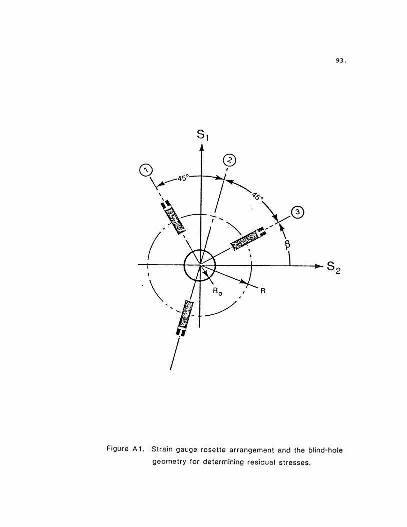
93.

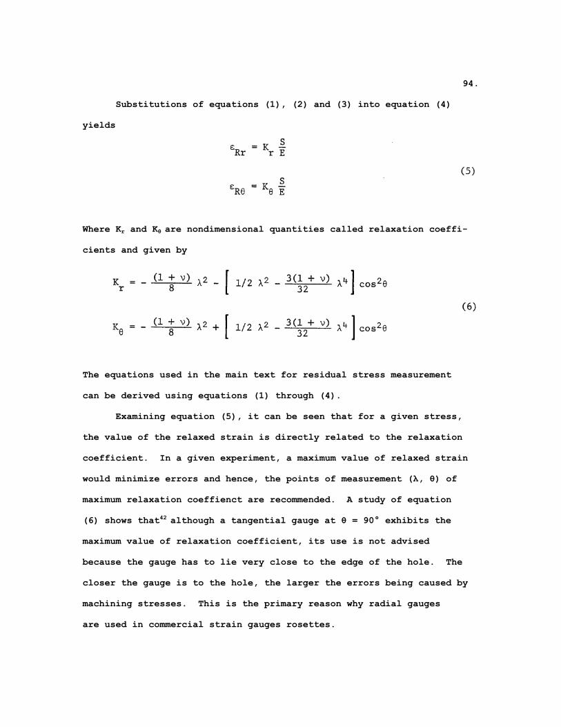
94.

Substitutions of equations (1), (2) and (3) into equation (4)

yields

Where Kr and Kθ are nondimensional quantities called relaxation coeffi-

cients and given by

The equations used in the main text for residual stress measurement

can be derived using equations (1) through (4).

Examining equation (5), it can be seen that for a given stress,

the value of the relaxed strain is directly related to the relaxation

coefficient. In a given experiment, a maximum value of relaxed strain

would minimize errors and hence, the points of measurement (λ, θ) of

maximum relaxation coeffienct are recommended. A study of equation

(6) shows that42 although a tangential gauge at θ = 90° exhibits the

maximum value of relaxation coefficient, its use is not advised

because the gauge has to lie very close to the edge of the hole. The

closer the gauge is to the hole, the larger the errors being caused by

machining stresses. This is the primary reason why radial gauges

are used in commercial strain gauges rosettes.

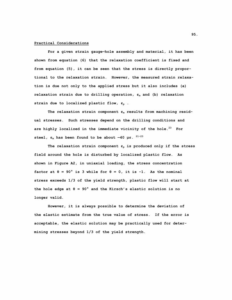
95. Practical Considerations

For a given strain gauge—hole assembly and material, it has been

shown from equation (6) that the relaxation coefficient is fixed and

from equation (5), it can be seen that the stress is directly propor-

tional to the relaxation strain. However, the measured strain relaxa-

tion is due not only to the applied stress but it also includes (a)

relaxation strain due to drilling operation, εm and (b) relaxation

strain due to localized plastic flow, εp .

The relaxation strain component εm results from machining resid-

ual stresses. Such stresses depend on the drilling conditions and

are highly localized in the immediate vicinity of the hole.23 For

steel, εm has been found to be about —40 με. 21-23

The relaxation strain component εp is produced only if the stress

field around the hole is disturbed by localized plastic flow. As

shown in Figure A2, in uniaxial loading, the stress concentration

factor at θ = 90° is 3 while for θ = 0, it is -1. As the nominal

stress exceeds 1/3 of the yield strength, plastic flow will start at

the hole edge at θ = 90° and the Kirsch’s elastic solution is no

longer valid.

However, it is always possible to determine the deviation of

the elastic estimate from the true value of stress. If the error is

acceptable, the elastic solution may be practically used for deter-

mining stresses beyond 1/3 of the yield strength.

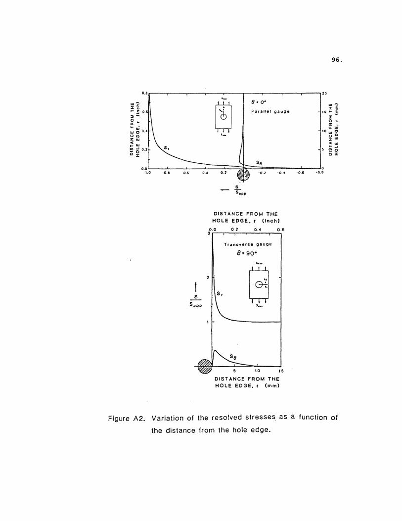
96.

97.

It can be seen that εp will always increase the absolute value of

the net relaxation strain, regardless of its sign. Thus, if the

relaxation strain εp is neglected, the measured stress, being tensile or

compressive, will always be overestimated. The presence of εp ,

being neglected, will lead to unrealistic and misleading results.

This may be illustrated with the aid of Figure A3. Assume that a

uniform stress Sapp > 1/3 Sy is measured by drilling a hole and record—

ing a total relaxation strain ac. If ac is considered entirely due to

the existing stress, direct substitution in equation (5) gives a

higher stress Sapp' = E/Kr ac.= E/Kr a’b’ , where line cb’ is drawn

parallel to elastic line. However, if εp = bc is realized, then the

true stress will be Sapp = E/Kr ab and the error in estimating Sapp

will be equal to bc / ab, i.e., εp / εRr . Similar analysis can be done

for a compressive stress. Correction for εp is required for stresses

that are in excess of 1/3 Sy or of a limit to be determined from

experiments.

Experimental

To determine the values of relaxation components εm and εp , two

6.35 mm thick annealed A—36 mild steel samples were used.

Specimen dimensions and strain gauge layout are shown in Figure A4.

A strain gauge rosette (type EA—06—125RE—l20) was bonded at the center

of the gauge length. The elements of this rosette are shown as 1, 2

and 3 in the figure. Four control gauges a, b, c and d (type EA—06—

125AD—l20) were also bonded, to measure the magnitude of the uniform

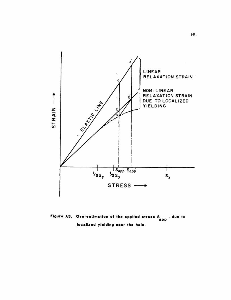
98.

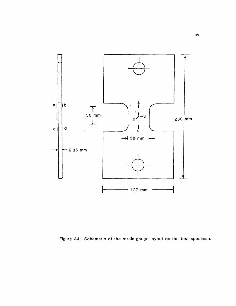
99.

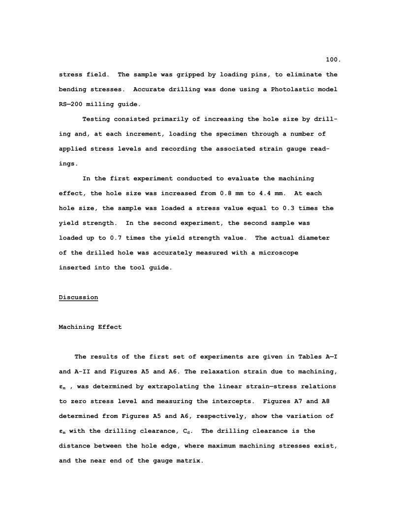
100.

stress field. The sample was gripped by loading pins, to eliminate the

bending stresses. Accurate drilling was done using a Photolastic model

RS—200 milling guide.

Testing consisted primarily of increasing the hole size by drill-

ing and, at each increment, loading the specimen through a number of

applied stress levels and recording the associated strain gauge read-

ings.

In the first experiment conducted to evaluate the machining

effect, the hole size was increased from 0.8 mm to 4.4 mm. At each

hole size, the sample was loaded a stress value equal to 0.3 times the

yield strength. In the second experiment, the second sample was

loaded up to 0.7 times the yield strength value. The actual diameter

of the drilled hole was accurately measured with a microscope

inserted into the tool guide.

Discussion

Machining Effect

The results of the first set of experiments are given in Tables A—I

and A-II and Figures A5 and A6. The relaxation strain due to machining,

εm , was determined by extrapolating the linear strain—stress relations

to zero stress level and measuring the intercepts. Figures A7 and A8

determined from Figures A5 and A6, respectively, show the variation of

εm with the drilling clearance, Cd. The drilling clearance is the

distance between the hole edge, where maximum machining stresses exist,

and the near end of the gauge matrix.

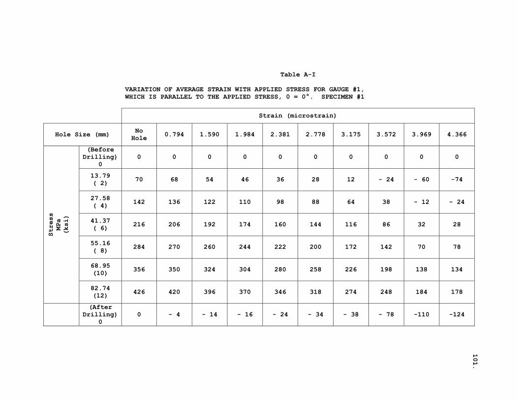
101.

Table A-I

VARIATION OF AVERAGE STRAIN WITH APPLIED STRESS FOR GAUGE #1, WHICH IS PARALLEL TO THE APPLIED STRESS, 0 = 0°. SPECIMEN #1

Strain (microstrain)

Hole Size (mm) No Hole 0.794 1.590 1.984 2.381 2.778 3.175 3.572 3.969 4.366

(Before Drilling)

0 0 0 0 0 0 0 0 0 0 0

13.79 ( 2) 70 68 54 46 36 28 12 - 24 - 60 -74

27.58 ( 4) 142 136 122 110 98 88 64 38 - 12 - 24

41.37 ( 6) 216 206 192 174 160 144 116 86 32 28

55.16 ( 8) 284 270 260 244 222 200 172 142 70 78

68.95 (10) 356 350 324 304 280 258 226 198 138 134

Stress

MPa

(ksi)

82.74 (12) 426 420 396 370 346 318 274 248 184 178

(After Drilling)

0 0 - 4 - 14 - 16 - 24 - 34 - 38 - 78 -110 -124

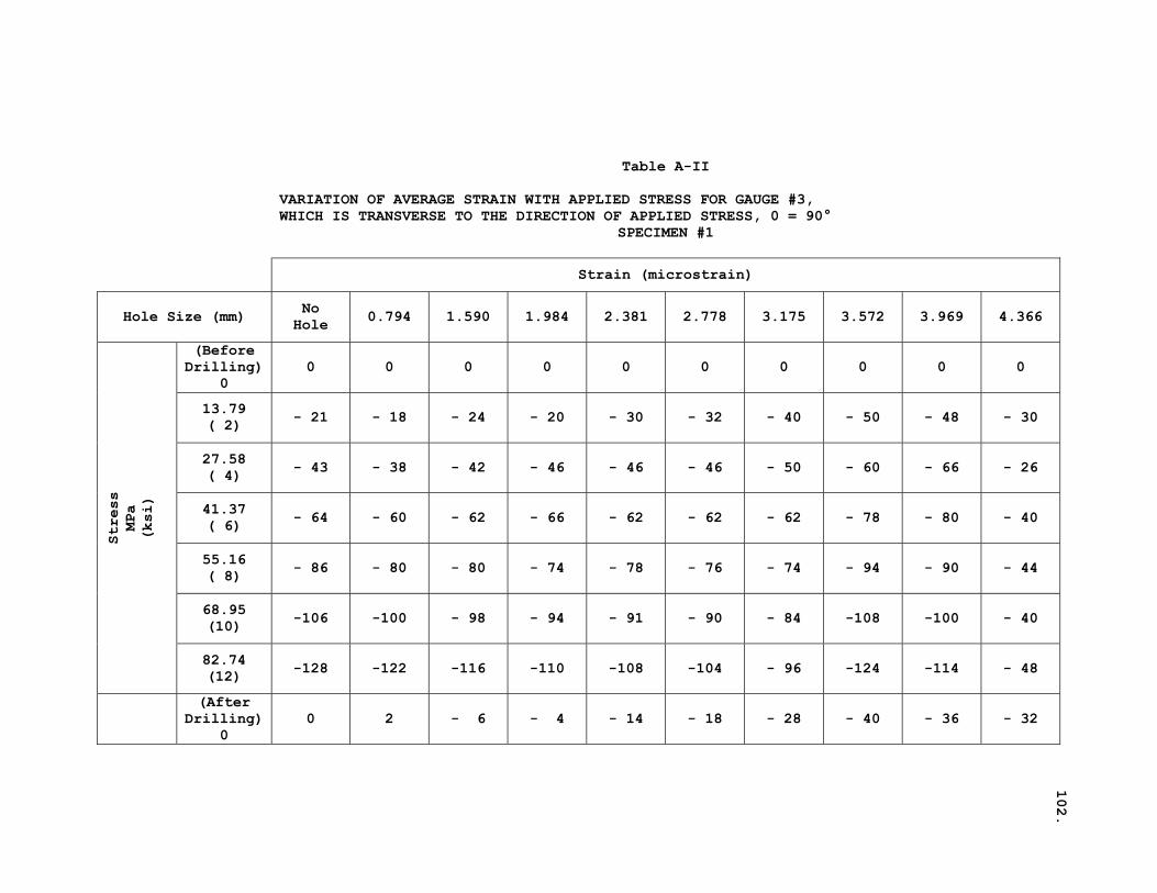
102.

Table A-II

VARIATION OF AVERAGE STRAIN WITH APPLIED STRESS FOR GAUGE #3, WHICH IS TRANSVERSE TO THE DIRECTION OF APPLIED STRESS, 0 = 90°

SPECIMEN #1 Strain (microstrain)

Hole Size (mm) No Hole 0.794 1.590 1.984 2.381 2.778 3.175 3.572 3.969 4.366

(Before Drilling)

0 0 0 0 0 0 0 0 0 0 0

13.79 ( 2) - 21 - 18 - 24 - 20 - 30 - 32 - 40 - 50 - 48 - 30

27.58 ( 4) - 43 - 38 - 42 - 46 - 46 - 46 - 50 - 60 - 66 - 26

41.37 ( 6) - 64 - 60 - 62 - 66 - 62 - 62 - 62 - 78 - 80 - 40

55.16 ( 8) - 86 - 80 - 80 - 74 - 78 - 76 - 74 - 94 - 90 - 44

68.95 (10) -106 -100 - 98 - 94 - 91 - 90 - 84 -108 -100 - 40

Stress

MPa

(ksi)

82.74 (12) -128 -122 -116 -110 -108 -104 - 96 -124 -114 - 48

(After Drilling)

0 0 2 - 6 - 4 - 14 - 18 - 28 - 40 - 36 - 32

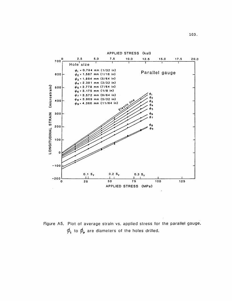
103.

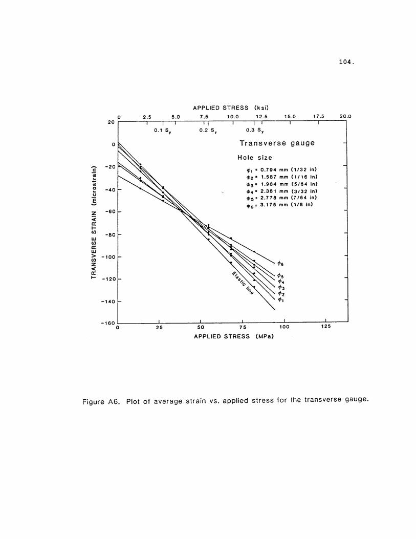
104.

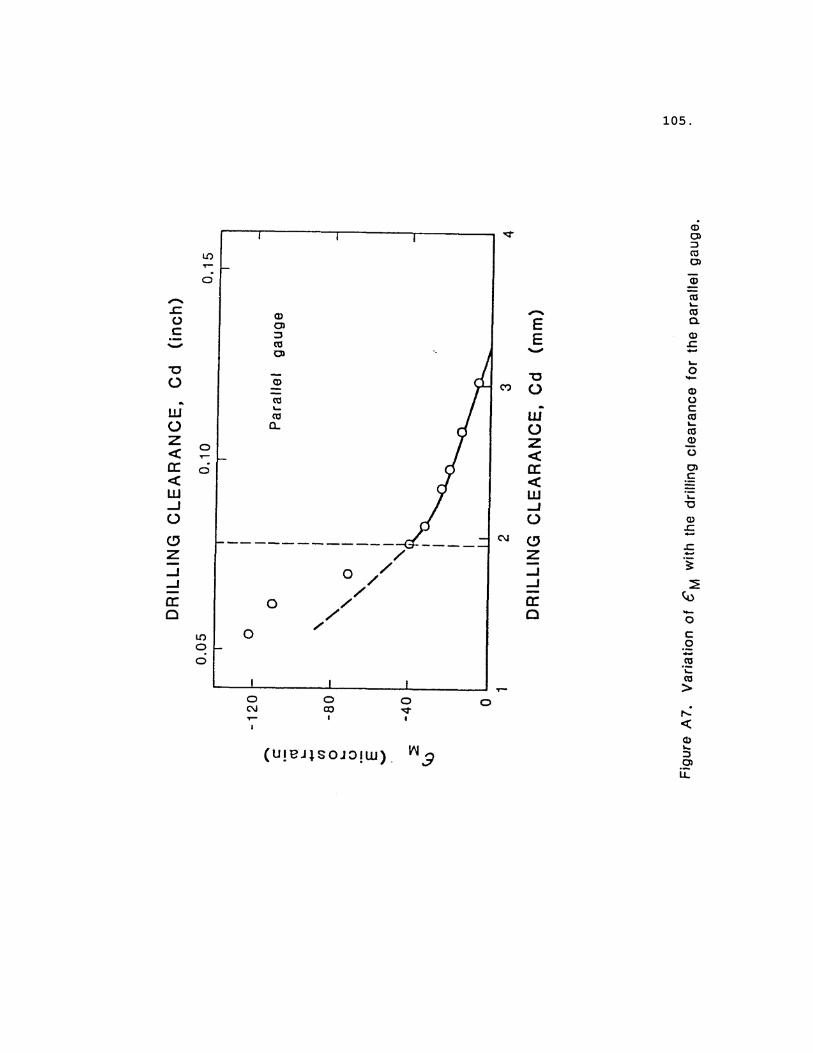
105.

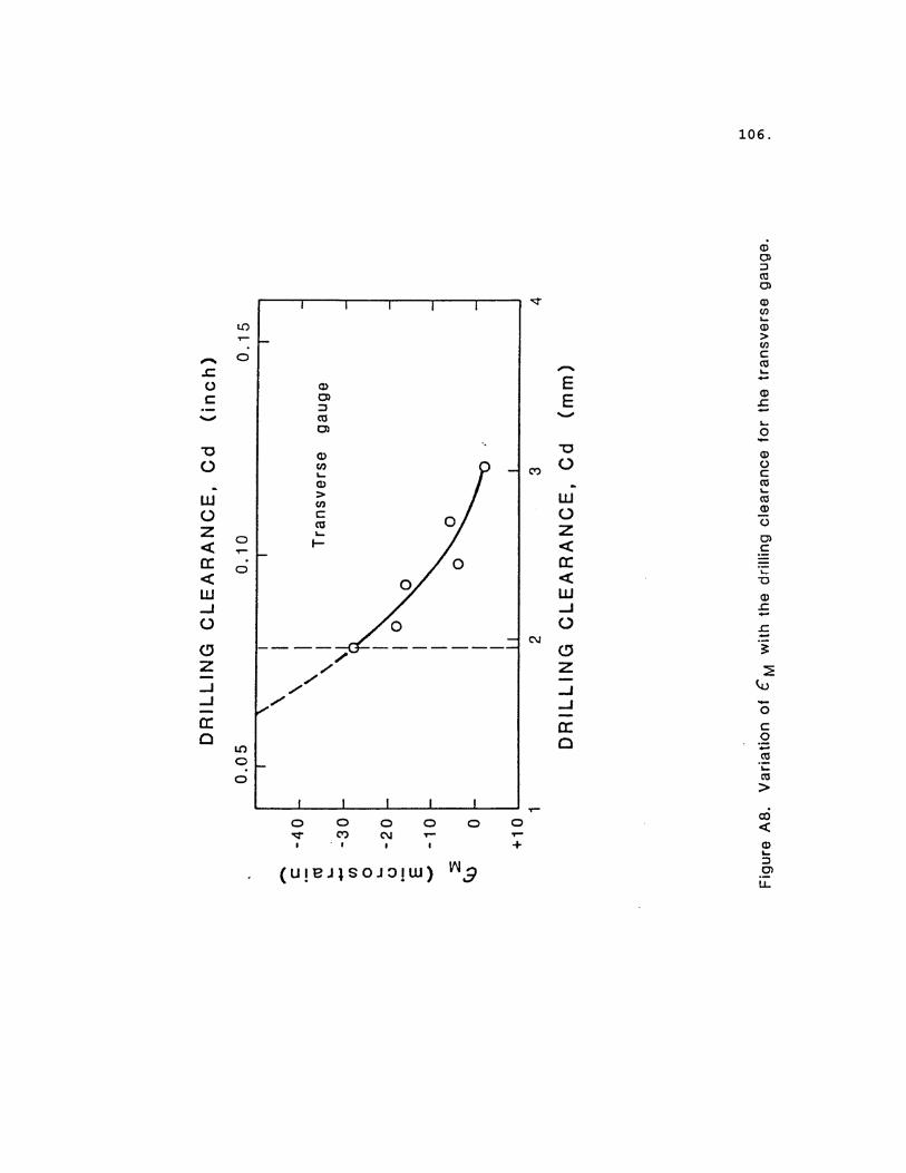
106.

107.

As mentioned before, the highly localized nature of machining

stresses is evident. In a situation where preformed strain gauge

rosettes cannot be used, precise locations of the strain gauges near

the hole are demanded. Hole diameter larger than the suggested 1/8

inch (3.175 mm) diameter, introduced abnormally high machining stresses

and hence, in the second set of experiments the maximum hole size was

limited to the suggested value of 3.175 mm. For this hole size, the

machining strains were —40 με and —30 με for gauges 1 and respectively.

Slightly lower values of εm for gauge 3 could be due to the transverse

sensitivity of the gauge. These values of εm for steel agree well with

the values obtained by others.21-23 Also, machining stresses seem to be

independent of the stress to be measured, since εm has the same sign

regardless of the sign of total relaxation strain.

Localized Plastic Flow Effect

The results of the second set of experiments are given in Tables

A—III and A—IV, and are plotted in Figures A9 and A10. An examination

of the results of Figures A9 and A10 suggests the following:

1. As the stress exceeds a certain value, the strain—stress

relations generally deviate from linearity causing the absolute value

of relaxation strain to increase. This critical stress is dependent

on the hole size and the strain gauge location, or more conveniently,

Cd. The locus of the critical stress that can be measured without

error due to localized plastic yielding at the hole edge is shown to

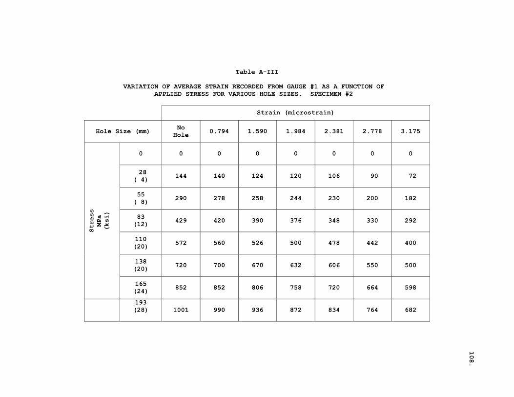
108.

Table A-III

VARIATION OF AVERAGE STRAIN RECORDED FROM GAUGE #1 AS A FUNCTION OF APPLIED STRESS FOR VARIOUS HOLE SIZES. SPECIMEN #2


Hole Size (mm) No Hole 0.794 1.590 1.984 2.381 2.778 3.175

0 0 0 0 0 0 0 0

28 ( 4) 144 140 124 120 106 90 72

55 ( 8) 290 278 258 244 230 200 182

83 (12) 429 420 390 376 348 330 292

110 (20) 572 560 526 500 478 442 400

138 (20) 720 700 670 632 606 550 500

Stress

MPa

(ksi)

165 (24) 852 852 806 758 720 664 598

193 (28)

1001 990 936 872 834 764 682

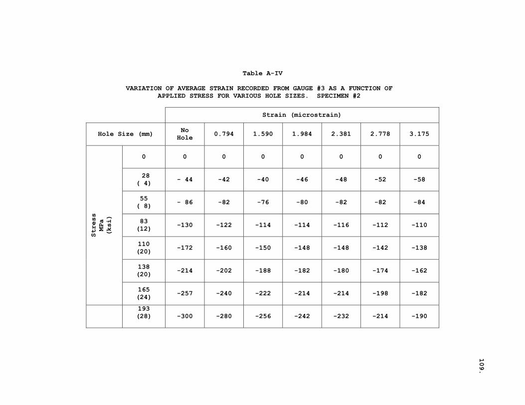
109.

Table A-IV

VARIATION OF AVERAGE STRAIN RECORDED FROM GAUGE #3 AS A FUNCTION OF APPLIED STRESS FOR VARIOUS HOLE SIZES. SPECIMEN #2


Hole Size (mm) No Hole 0.794 1.590 1.984 2.381 2.778 3.175

0 0 0 0 0 0 0 0

28 ( 4) - 44 -42 -40 -46 -48 -52 -58

55 ( 8) - 86 -82 -76 -80 -82 -82 -84

83 (12) -130 -122 -114 -114 -116 -112 -110

110 (20) -172 -160 -150 -148 -148 -142 -138

138 (20) -214 -202 -188 -182 -180 -174 -162

Stress

MPa

(ksi)

165 (24) -257 -240 -222 -214 -214 -198 -182

193 (28)

-300 -280 -256 -242 -232 -214 -190

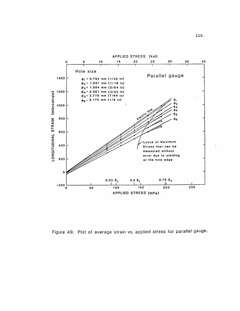
110.

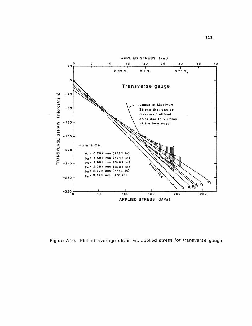
111.

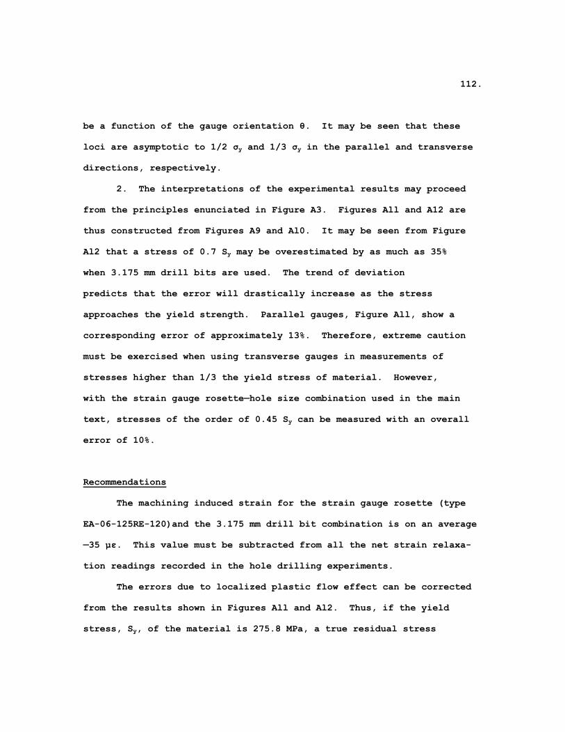
112.

be a function of the gauge orientation θ. It may be seen that these

loci are asymptotic to 1/2 σy and 1/3 σy in the parallel and transverse

directions, respectively.

2. The interpretations of the experimental results may proceed

from the principles enunciated in Figure A3. Figures All and A12 are

thus constructed from Figures A9 and Al0. It may be seen from Figure

Al2 that a stress of 0.7 Sy may be overestimated by as much as 35%

when 3.175 mm drill bits are used. The trend of deviation

predicts that the error will drastically increase as the stress

approaches the yield strength. Parallel gauges, Figure All, show a

corresponding error of approximately 13%. Therefore, extreme caution

must be exercised when using transverse gauges in measurements of

stresses higher than 1/3 the yield stress of material. However,

with the strain gauge rosette—hole size combination used in the main

text, stresses of the order of 0.45 Sy can be measured with an overall

error of 10%.

Recommendations

The machining induced strain for the strain gauge rosette (type

EA-06-125RE-120)and the 3.175 mm drill bit combination is on an average

—35 με. This value must be subtracted from all the net strain relaxa-

tion readings recorded in the hole drilling experiments.

The errors due to localized plastic flow effect can be corrected

from the results shown in Figures All and Al2. Thus, if the yield

stress, Sy, of the material is 275.8 MPa, a true residual stress

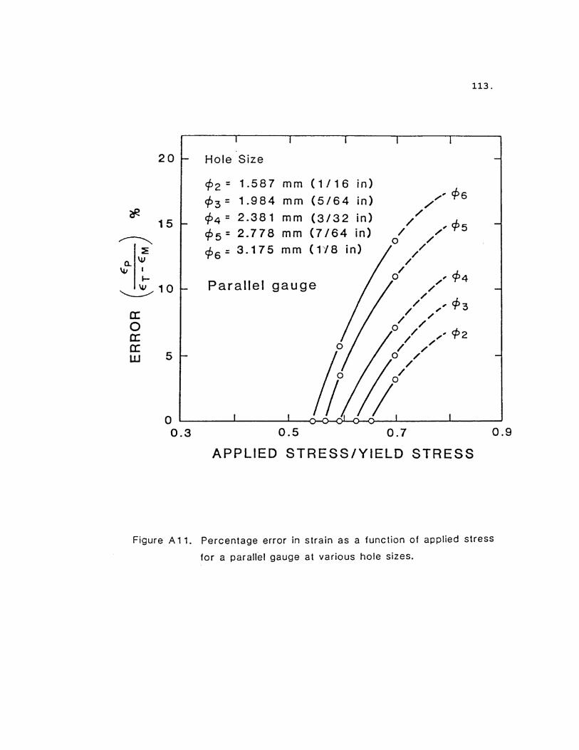
113.

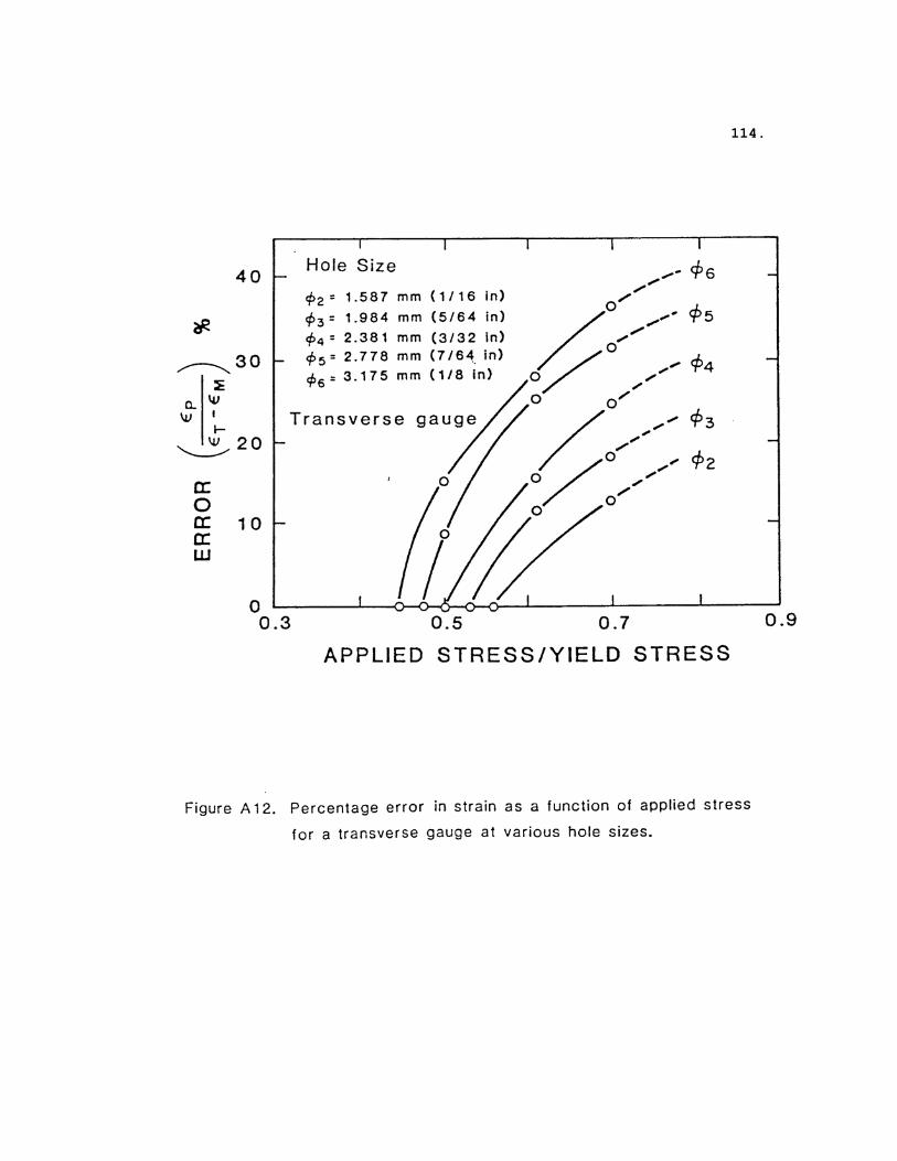
114.

115.

of 193.1 MPa, which is 0.7 Sy, will be exaggerated by about 35% to a

value of 262 MPa by a transverse gauge, whereas a parallel gauge will

exaggerate it to about 220.6 MPa.

For example, consider the reading from rosette #1 of weldment 1

in the as—welded condition. In the following Table A—V, the successive

changes in the stress that occur as a result of modification of the

three relaxed strains are shown.

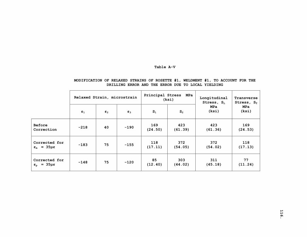
116.

Table A-V

MODIFICATION OF RELAXED STRAINS OF ROSETTE #1, WELDMENT #1, TO ACCOUNT FOR THE DRILLING ERROR AND THE ERROR DUE TO LOCAL YIELDING

Relaxed Strain, microstrain Principal Stress MPa (ksi)

ε1 ε2 ε3 S1 S2


MPa (ksi)

TransverseStress, ST

MPa (ksi)

Before Correction -218 40 -190 169

(24.50) 423

(61.39) 423

(61.36) 169

(24.53)

Corrected for εm = 35με

-183 75 -155 118 (17.11)

372 (54.05)

372 (54.02)

118 (17.13)

Corrected for εp = 35με

-148 75 -120 85 (12.40)

303 (44.02)

311 (45.18)

77 (11.24)

117.

BIOGRAPHICAL NOTE

The author was born in Bangalore, India, on March 8, 1952. He

received his B.Sc. degree in 1971 from Bangalore University and his

B.E. degree in Metallurgy in 1974 from Indian Institute of Science,

Bangalore, India.

In 1975, he began graduate work at the Oregon Graduate Center.

Documents

The Vibratory Stress Relief Library - VSR Technology · VIBRATORY STRESS RELIEF OF MILD STEEL WELDMENTS S. Shankar B.S., Bangalore University, India, 1971 B.E., Indian Institute of