Thermoacoustic Heat Engine Modelingand Design Optimization∗

Andrew C. Trapp† Florian Zink‡ Oleg A. Prokopyev§

Laura Schaefer¶

July 27, 2011

Abstract

Thermoacoustic heat engines (TAEs) are potentially advantageous drivers for ther-moacoustic refrigerators (TARs). Connecting TAEs to TARs means that waste heatcan effectively be utilized to provide cooling, and increase overall efficiency. However,this is currently a niche technology. Improvements can be made through a better un-derstanding of the interactions of relevant design parameters. This work develops anovel mathematical programming model to optimize the performance of a simple TAE.The model consists of system parameters and constraints that capture the underlyingthermoacoustic dynamics. We measure the performance of the engine with respect toseveral acoustic and thermal objectives (including work output, viscous losses and heatlosses). Analytical solutions are presented for cases of single objective optimization thatidentify globally optimal parameter levels. We also consider optimizing multiple ob-jective components simultaneously and generate the efficient frontier of Pareto optimalsolutions corresponding to selected weights.

Keywords: Thermoacoustics; Mathematical Programming; Global Optimization;Multiobjective Optimization; Efficient Frontier

1 Introduction

The goal of this work is to demonstrate how optimization techniques can improve the designof thermoacoustic devices. Thermoacoustic devices utilize sound waves instead of mechanicalpistons to drive a thermodynamic process. One of their advantages is the inherent mechani-cal simplicity. While this concept is not new, the technology has not been advanced to a highdegree, as compared to, for example, the internal combustion engine. After reviewing some

∗Corresponding author: O.A. Prokopyev. E-mail: prokopyev@engr.pitt.edu†Worcester Polytechnic Institute, School of Business, Worcester, MA 01609‡IAV GmbH, Rockwellstr. 16, 38518 Gifhorn, Germany§Department of Industrial Engineering, University of Pittsburgh, Pittsburgh, PA 15261¶University of Pittsburgh, Department of Mechanical Engineering and Material Science, 153 Benedum

Hall, Pittsburgh, PA 15261

1

fundamental physical properties underlying thermoacoustic devices, we will then proceed todiscuss our approach to optimize their design.

The Stirling cycle, developed in 1816 Garrett [1999], is the basic thermodynamic cycleoccurring in thermoacoustic devices. The original mechanical Stirling engine utilized twopistons and a regenerative heat exchanger Kaushik and Kumar [2000]. Over the course ofone cycle, the working gas is compressed; it then transfers thermal energy to the heat sink,thus maintaining a constant temperature. Afterwards, the gas is heated at constant volumeby the regenerator and then is heated further at the heat source. This heat supply occurswhile the gas is allowed to expand and drive the power piston, again at constant temperature.After expansion, the gas is displaced to the heat sink, while cooling off at constant volume bydepositing heat to the regenerator, which stores heat between cycle segments Kaushik andKumar [2000]. It is noteworthy that this externally heated, closed cycle uses the same gas forall stages, as opposed to the internal combustion engine, which has a constant throughputof working gas and fuel. The first application of this cycle as a thermoacoustic technologyoccurred when Ceperley recognized that sound waves could replace pistons for gas compres-sion and displacement Ceperley [1985]. Since then, a wide variety of thermoacoustic engines(TAEs) and their counterpart, thermoacoustic refrigerators (TARs), have been developed.TAEs utilize a heat input to create intense sound output, while TARs can utilize this intensesound to withdraw energy from their surroundings.

1.1 Thermoacoustic Engines

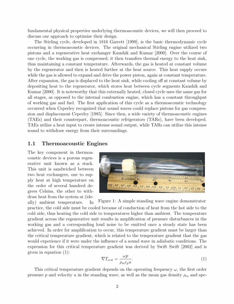
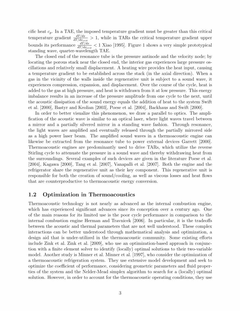
Figure 1: A simple standing wave engine demonstrator

The key component in thermoa-coustic devices is a porous regen-erative unit known as a stack.This unit is sandwiched betweentwo heat exchangers, one to sup-ply heat at high temperature onthe order of several hundred de-grees Celsius, the other to with-draw heat from the system at (ide-ally) ambient temperature. Inpractice, the cold side must be cooled because of conduction of heat from the hot side to thecold side, thus heating the cold side to temperatures higher than ambient. The temperaturegradient across the regenerative unit results in amplification of pressure disturbances in theworking gas and a corresponding loud noise to be emitted once a steady state has beenachieved. In order for amplification to occur, this temperature gradient must be larger thanthe critical temperature gradient, which is related to the temperature gradient that the gaswould experience if it were under the influence of a sound wave in adiabatic conditions. Theexpression for this critical temperature gradient was derived by Swift Swift [2002] and isgiven in equation (1):

∇Tcrit =ωp

ρmcpu. (1)

This critical temperature gradient depends on the operating frequency ω, the first orderpressure p and velocity u in the standing wave, as well as the mean gas density ρm and spe-

2

cific heat cp. In a TAE, the imposed temperature gradient must be greater than this critical

temperature gradient dT/dxdT/dxcrit

> 1, while in TARs the critical temperature gradient upper

bounds its performance dT/dxdT/dxcrit

< 1 Xiao [1995]. Figure 1 shows a very simple prototypicalstanding wave, quarter-wavelength TAE.

The closed end of the resonance tube is the pressure antinode and the velocity node; bylocating the porous stack near the closed end, the interior gas experiences large pressure os-cillations and relatively small displacement. A heating wire provides the heat input, causinga temperature gradient to be established across the stack (in the axial direction). When agas in the vicinity of the walls inside the regenerative unit is subject to a sound wave, itexperiences compression, expansion, and displacement. Over the course of the cycle, heat isadded to the gas at high pressure, and heat is withdrawn from it at low pressure. This energyimbalance results in an increase of the pressure amplitude from one cycle to the next, untilthe acoustic dissipation of the sound energy equals the addition of heat to the system Swiftet al. [2000], Bastyr and Keolian [2003], Poese et al. [2004], Backhaus and Swift [2000].

In order to better visualize this phenomenon, we draw a parallel to optics. The ampli-fication of the acoustic wave is similar to an optical laser, where light waves travel betweena mirror and a partially silvered mirror in a standing wave fashion. Through resonance,the light waves are amplified and eventually released through the partially mirrored sideas a high power laser beam. The amplified sound waves in a thermoacoustic engine canlikewise be extracted from the resonance tube to power external devices Garrett [2000].Thermoacoustic engines are predominantly used to drive TARs, which utilize the reverseStirling cycle to attenuate the pressure in a sound wave and thereby withdrawing heat fromthe surroundings. Several examples of such devices are given in the literature Poese et al.[2004], Kagawa [2000], Tang et al. [2007], Vanapalli et al. [2007]. Both the engine and therefrigerator share the regenerative unit as their key component. This regenerative unit isresponsible for both the creation of sound/cooling, as well as viscous losses and heat flowsthat are counterproductive to thermoacoustic energy conversion.

1.2 Optimization in Thermoacoustics

Thermoacoustic technology is not nearly as advanced as the internal combustion engine,which has experienced significant advances since its conception over a century ago. Oneof the main reasons for its limited use is the poor cycle performance in comparison to theinternal combustion engine Herman and Travnicek [2006]. In particular, it is the tradeoffsbetween the acoustic and thermal parameters that are not well understood. These complexinteractions can be better understood through mathematical analysis and optimization, adesign aid that is under-utilized in the thermoacoustic community. Some existing effortsinclude Zink et al. Zink et al. [2009], who use an optimization-based approach in conjunc-tion with a finite element solver to identify (locally) optimal solutions to their two-variablemodel. Another study is Minner et al. Minner et al. [1997], who consider the optimization ofa thermoacoustic refrigeration system. They use extensive model development and seek tooptimize the coefficient of performance, considering geometric parameters and fluid proper-ties of the system and the Nelder-Mead simplex algorithm to search for a (locally) optimalsolution. However, in order to account for the thermoacoustic operating conditions, they use

3

DeltaE extensively. DeltaE is a blackbox simulation tool based on linear acoustic theory de-veloped by Swift et al. Swift [2002] that considers a thermoacoustic device as a combinationof individual sections. It analyzes each section in regard to its acoustic properties and thevelocity, pressure, and temperature behavior.

Both Wetzel Wetzel [1998] and Besnoin Besnoin [2001] discuss thermoacoustic deviceoptimization in their works. While Wetzel focuses on the optimal performance of a ther-moacoustic refrigerator, Besnoin targets heat exchangers. In addition to these optimizationefforts, Zoontjens Zoontjens et al. [2006] illustrates the optimization of inertance sectionsof thermoacoustic devices; they also use DeltaE to vary individual parameters to determineoptimal designs. Ueda Ueda et al. [2003] determines the effect of a variation of certain en-gine parameters on pressure amplitudes. Another work that makes use of DeltaE is Tijaniet al. Tijani et al. [2002], who attempt to optimize the spacing of the stack.

1.3 Goals of the present work

While the previous works are valuable additions to the field of thermoacoustics, most studies(the exception being the Zink et al. Zink et al. [2009] and Minner et al. Minner et al. [1997]studies) vary only a single parameter, holding all else fixed. Such parametric studies are un-able to capture the nonlinear interactions inherent in thermoacoustic models with multiplevariables, and can only guarantee locally optimal solutions. In contrast, our model allowsfor the simultaneous varying of multiple parameters to identify globally optimal values. Ad-ditionally, our model considers several contrasting acoustic and thermal objectives, whereunlike previous studies we incorporate heat losses to the surroundings occurring with normaldevice operation. Because optimizing with respect to such losses may be less intuitive thanthe more obvious goals of maximizing power output or efficiency, we provide a magnitudeestimate in Section 2.1.2 to justify their inclusion. The presence of these contrasting objec-tives permits the additional modeling flexibility of using weights to place desired objectivecomponent emphasis in the context of multiobjective optimization (see also discussion inSection 2.1). Optimal solutions corresponding to specific objective weights can be used toconstruct the efficient frontier of Pareto optimal solutions.

The remainder of this paper is organized in the following fashion: the fundamental com-ponents of our mathematical model characterizing the standing wave thermoacoustic Sterlingheat engine are presented in Section 2. In Section 3, we discuss single objective optimization,using analytical approaches to find values of the variables that satisfy the constraints andare globally optimal with respect to the considered objective function. Section 4 considersmultiobjective optimization. In Section 5, we conclude by suggesting possible future exten-sions of this work, and in Section 7 we provide a concise summary of the key terminologyused in this paper.

2 TAE Modeling

In this section we describe the mathematical model we use to represent the underlying dy-namics of thermoacoustic systems.

4

2.1 Model Components

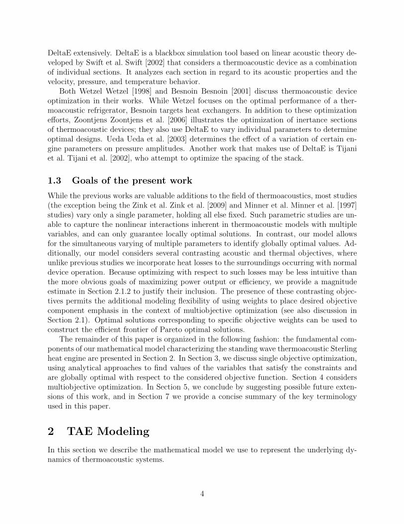
In the following sections we discuss our modeling approaches for the physical standing waveengine depicted in Figure 2, including our development of a mathematical model and itscorresponding optimization. We reduce our problem domain to two dimensions by takingadvantage of the symmetry present in the stack. To account for the thermal behavior of thedevice, the reduced domain is given two constant temperature boundaries, one convectiveboundary, and one adiabatic boundary. In the thermal calculations, we are primarily inter-ested in the temperature distribution achieved in the domain, and discuss several approachesto determine the relevant temperature profiles. Acoustically, we represent the stack’s workflow and viscous resistance using expressions constructed from several structural variables,that are in turn involved in a number of structural constraints. The variables are the param-eters1that we allow to be varied, while structural constraints are equations and inequalitiesthat enforce restrictions on permissible variable combinations. We measure the quality of agiven set of variable values that satisfies all of the constraints using an objective function.

Multiobjective optimization is concerned with the optimization of more than one objec-tive function that are conflicting in nature Miettinen [1999]. They are conflicting in thesense that, if optimized individually, they do not share the same optimal solutions. Whenoptimizing multiple objective components simultaneously, each objective is given a weightto allow the user to place desired emphasis. In this context, a Pareto optimal solution is onein which there does not exist another solution which strictly improves one of the consideredobjective components without worsening another objective component. Thus, by varyingthe weighted emphasis on objective components, multiple Pareto optimal solutions can beobtained and in turn be used to generate the efficient frontier.

2.1.1 Variables

We characterize the fundamental properties of the stack using the following five structuralvariables:

• L: Stack length,

• H: Stack height,

• Z: Stack placement,

• dc: Channel diameter, and

• N : Number of channels.

Each variable has positive lower and upper bounds and is depicted in Figure 2. Both thestack length L and height H take real values between their bounds, where the stack height isdefined as the radius of a cross section of the resonance tube. The placement of the stack inthe axial direction of the resonator is modeled by continuous variable Z; near the closed end

1We differentiate between the terms variables and parameters, in that we use the term variables toindicate the structural components we allow to fluctuate in order to improve the objective, and the termparameters to indicate either known quantities (i.e., constants) or auxiliary quantities that are completelydependent on the values of the structural variables and other constant parameters.

5

of the resonance tube its value approaches 0 from above. We take the maximum length of theresonator tube to be a quarter-wavelength, i.e., Zmax = λ

4, implying that Z can effectively

range from Zmin to Zmax−L to properly account for the stack length. Because the geometryof the porous stack is based on the monolith structure used in experimentation Zink et al.[2009], we model it using square channels, representing the channel size with continuousvariable dc, so that the channel perimeter Πc = 4dc and area Ac = d2c . We allow dc to rangefrom the thermal penetration depth δκ to Fδκ, where F is an integer-valued multiplier on thethermal penetration depth. If the size of the stack’s channels is too large, the key interactionbetween the gas and the wall does not occur, thus hindering the amplification of acousticwaves Swift [2002]; hence we take F to be 4 because it results in a channel dimension thatstill yields thermoacoustic performance. Finally, we model the number of channels N withinthe stack as an integer-valued variable.

Convection/Radiation

Conduction

Adiabatic

Thot Tcold

dc

Z

zL

r

ϕ

Z=0

Z=λ/4

H

N

}

Figure 2: Computational domain and boundary conditions illustrating L, H, Z, N , dc

2.1.2 Objectives

We consider multiple components in the objective function of our optimization model. Em-phasizing power is prominent in the design of energy systems; this also justifies the optimiza-tion of the stack with regard to its viscous performance. We rely upon physical observationsto provide justification with respect to thermal behavior. When one side of the stack isheated to approximately 300◦C using about 50 W of electrical input, the temperature ofthe opposite side measures 50◦C. This temperature gradient yields a conductive heat fluxthat must be considered a loss. It is directly proportional to the stack’s material (and thusthermal conductivity). We also account for the thermal losses through the shell of our ther-moacoustic device. This is a less obvious source of loss in thermoacoustic devices, but mustalso be considered. Accounting for the dimensions and material properties of our smalldemonstrator engine, a cursory estimate of these losses is approximately 20 % of the total

6

input power. This magnitude justifies our motivation to optimize the geometry of the stackto minimize the three aforementioned thermal losses.

Our final objective function is a combination of the following five individual components:

• W : Work output,

• Rν : Viscous resistance,

• Qconv: Convective heat flow,

• Qrad: Radiative heat flow, and

• Qcond: Conductive heat flow.

Each objective component has a weighting factor wi to provide appropriate user-definedemphasis. The two acoustic objectives are the work output W of the thermoacoustic engineand the viscous resistance Rν through the stack Swift [2002, 1988]. The thermal objectivesinclude both the convective heat flow Qconv and the radiative heat flow Qrad, which we eval-uate at the top boundary of the stack, as well as the conductive heat flow Qcond, which isevaluated at the end of the resonance tube. Because work is the only objective to be max-imized, we instead minimize its negative magnitude along with all of the other components.

As is typical in multiobjective optimization, the objective function components in ourmodel are conflicting and of vastly different magnitudes and units. We can restore this im-balance by incorporating normalization factors on each component weight wi. Thus, withoutloss of generality, we make the assumption that weights wi are normalized in our followingdiscussions, which makes each objective function component unitless and nonnegative inmagnitude. Section 4.1 provides further details on our procedure to normalize the objectivefunction components.

2.1.3 Structural Constraints

In addition to having lower and upper bounds, variables may only take values that satisfycertain physical properties governing the engine. One such property is that the total numberof channels N of a given diameter dc is limited by the cross-sectional radius of the resonancetube H. This relationship yields the constraint AN(dc+tw)2 ≤ πH2, where tw represents thewall thickness around a single channel, and A represents the ratio of the area of a filled circleto its optimal packing by smaller square channels. From observations on optimal packings(see, e.g., Friedman), 1 ≤ A ≤ 1.5, so we set A = 1.25. Other model constraints equateauxiliary parameters used in the optimization.

2.2 Mathematical Programming Formulation

We present our mathematical model (MPF) in this section. Taken together, expressions (2)– (27) represent a nonlinear mixed-integer program.

(MPF) minL,H,Z,dc,N

ζ = w1(−W ) + w2Rν + w3Qconv + w4Qrad + w5Qcond (2)

7

subject toAN(dc + tw)2 ≤ πH2, (3)

W =Πcω

4

[δκ

(γ − 1)p2

ρc2(1 + ε)(Γ− 1)− δνρu2

]LN = ω

[δκ

(γ − 1)p2

ρc2(1 + ε)(Γ− 1)− δνρu2

]LNdc,

(4)

Rν =µΠc

A2cδν

L

N=

4µ

δν

L

Nd3c, (5)

Qconv = H

∫ 2π

0

∫ L

0

h(Ts) (Ts − T∞) dzdϕ, (6)

Qrad = H kb

∫ 2π

0

∫ L

0

ε(T 4s − T 4

∞)dzdϕ, (7)

Qcond =

∫ 2π

0

∫ H

0

(krr

∂T

dr+ kzz

∂T

dz

)drdϕ, (8)

Qcond|z=Lmax =

∫ 2π

0

∫ H

0

(kzz

∂T

∂z

)drdϕ. (9)

Heat flow equations (6) – (9) depend on the following additional parameters:

h(Ts) =kg2H

Nu, (10)

Nu = 0.36 +0.518Ra

14D[

1 + (0.559Pr

)916

] 49

, (11)

RaD = Gr Pr =gβ(Ts − T∞)

να(2H)3, (12)

Pr =ν

α, (13)

krr =kskg(tw + dc)

kstw + kgdc, (14)

kzz =kstw + kgdctw + dc

. (15)

The work expression (4) depends on the following four parameters:

ε =(ρcpδκ)g(ρcpδs)s

tanh ((i+ 1)y0/δκ)

tanh ((i+ 1)l/δs), (16)

umax =pmaxρc

, (17)

p = pmax cos

(2πZ

λ

), (18)

8

u = umax sin

(2πZ

λ

). (19)

The variables are subject to the following restrictions:

Lmin ≤ L ≤ Lmax, (20)

Hmin ≤ H ≤ Hmax, (21)

δκ ≤ dc ≤ Fδκ, (22)

Zmin ≤ Z ≤ Zmax − L, (23)

Nmin ≤ N ≤ Nmax, (24)

L, H, Z, dc ∈ R+;N ∈ Z+. (25)

The following boundary conditions must also be enforced:

1. Constant hot side temperature (Th),

2. Constant cold side temperature (Tc),

3. Adiabatic boundary, modeling the central axis of the cylindrical stack:

∂T

dr

∣∣∣∣r=0

= 0, and (26)

4. Free convection and radiation to surroundings (at T∞) with temperature dependentheat transfer coefficient (h), emissivity (ε), and thermal conductivity (k):

k∂T

dr

∣∣∣∣r=H

= h (Ts − T∞) + εkb(T 4s − T 4

∞). (27)

We denote by x the solution vector of structural variables, i.e., x = [L,H, dc, Z,N ]. Con-straint (3) relates the channel diameter dc and the number of possible channels N to theradius H of the cross-sectional area, while equations (4) – (8) express our five objective func-tion components of interest. Equations (4) and (5) calculate the work W and viscous resis-tance Rν , respectively, as functions of L, dc, Z, and N (and indirectly H through (3)). Equa-tions (6) – (9) represent heat flows. Equations (10) – (19) solve for parameters used in objec-tive function components, (20) – (25) restrict variables values, and (26) – (27) represent heatflow boundary conditions. Note that umax and pmax are related2 at zo = 0 as shown in (17).

Remark 1 In equation (16), the real part of ε is observed to tend to√32

, and we set ε tothis value.

Remark 2 We set the hot-side temperature Th = ∇TL + Tc, where ∇T and Tc are prede-termined values. Note that the constant temperature gradient ∇T is an approximation andits validity is assumed over the entire domain of structural variables (i.e., L ∈ [Lmin, Lmax],H ∈ [Hmin, Hmax], etc.). This behavior corresponds with experimental observations thatclearly indicate a positive correlation between the stack length L and hot side temperature Thin order to successfully sustain the thermoacoustic energy conversion. Additional details canbe found in Section 2.3.1.

9

Remark 3 While the heat transfer coefficient h, in this case for natural convection, dependson the surface temperature Ts (a function of z), this value is calculated separately and treatedas constant; see Section 2.3.2 for a related discussion.

Remark 4 We assume that constraint (3) is satisfied when variables H, N , and dc are attheir lower bounds, so that ANmin(dcmin + tw)2 ≤ πH2

min holds.

2.3 Approximating the Heat Flows

We next discuss how we arrived at equations (6) – (9), (26), and (27), including theirapproximation.

2.3.1 Estimating the Temperature Distribution

Given an input H (and L), it is necessary to find the solution of the 2D temperature distri-bution in our reduced domain, subject to boundary conditions detailed above. Due to thenature of the boundary conditions, the analytical solution is very difficult. Numerical solverssuch as COMSOL Multiphysics COM [2005], MATLAB Finite Element Toolbox Mat [2007],etc. are another option to determine the temperature distribution. However, this precisioncomes at high computational cost. Considering that the temperature distribution is requiredfor the estimation of the heat fluxes, only the temperature distribution at the shell surfaceand the temperature gradient at the cold side are of interest. For this purpose it is reason-able to reduce the temperature calculations to those two relevant values. The temperaturedistribution along the top surface can be well-approximated by an exponentially decayingtemperature distribution throughout the domain. This behavior was determined throughan analysis of the finite element solution. The final surface temperature distribution as afunction of axial direction z is given by:

Ts = Theln(TcTh

)zL . (28)

This distribution is assumed to be valid on the surface characterized by (z, r = H) andapproximates the physical temperature distribution. This same temperature distribution isused to determine the axial temperature gradient at the cold side (required for the conductiveheat flux). Considering again the rectangular domain, we can see that the temperaturegradient in the center (i.e. bottom, r = 0) will vary linearly from Th to Tc. Assumingthat the temperature gradient at the cold side is exponential for all r will result in anunderestimation of the conductive heat flux.

2.3.2 Determining the Heat Fluxes

The temperature distribution stated in equation (28) is then used to determine the convectiveand radiative heat transfer to the surroundings via:

Qconv = 2πHh

L∫0

(Ts − T∞) dz. (29)

2pmax is determined either by an informed choice based on domain knowledge, or via simulation.

10

As noted in Remark 3, the temperature dependent heat transfer coefficient h(T ) is deter-mined in a preprocessor (derived from the appropriate Nusselt law, as stated in equation (11)and an average surface temperature), and is not considered as part of the integral. The ra-diative heat transfer (in the general case) is written as:

Qrad = 2πHkBε

L∫0

(T 4s − T 4

∞)dz, (30)

which depends on the surface emissivity ε and Stefan-Boltzmann constant kB, both ofwhich are assumed to be independent of temperature.

After integrating we derive the following heat flow expressions:

Qconv = 2πHLh

Th

ln(TcTh

) (TcTh− 1

)− T∞

, and (31)

Qrad = 2πHLkBε

T4h

(e4ln

(TcTh

)− 1

)4ln(TcTh

) − T 4∞

. (32)

In the present case, this approximation of the temperature distribution (equation (28)) isalso utilized to determine the conductive heat flow at z = L. The temperature distributionthroughout the 2D domain implies that this estimate will fall between the extremes of:

1. the physical case (under anisotropic material properties and physical boundary condi-tions), and

2. the assumption of constant temperature gradient determined as dTdz

= Th−TcL

, as thelatter case only exists at the adiabatic boundary z, r = 0 and quickly loses validity.

At the top surface z, r = H the exponential distribution is assumed, so we determinethe temperature gradient using this temperature distribution. Determining

∂T

∂z

∣∣∣∣z=L

=TcLln

(TcTh

)(33)

and implementing this in the general statement of the Fourier law of thermal conduction,we can express this heat flow as:

Qcond =kzzLπH2Tcln

(ThTc

). (34)

This expression for the conductive heat flow depends on the effective thermal conductivityin the z-direction as defined in equation (15). Using mild assumptions, equations (31), (32)and (34) give expressions for the heat flows that, while still nonlinear, no longer requireexternal finite element solvers to evaluate.

11

3 Single Objective Optimization

We have presented a mathematical model that characterizes the essential elements of astanding wave thermoacoustic engine. Based on the discussion in Section 2.3.2, our nonlinearmodel can be solved independently of finite element solvers. In the following discussion weanalyze restricted cases of our objectives, and identify general tendencies of the structuralvariables to influence individual objective components.

3.1 Acoustic Emphasis

The following two sections analyze the cases where objective function (2) is restricted tooptimizing work and viscous resistance, respectively.

3.1.1 Emphasizing Work

Setting the objective function weights to w2 = w3 = w4 = w5 = 0 and w1 = 1, the problemreduces to constraints (3), (4), (17) – (19), and variable restrictions (20) – (25). Objectivefunction (2) becomes:

minL,H,dc,Z,N

ζW = (−W ). (35)

By incorporating (17) – (19) into the initial term of equation (4) (which is a function ofZ through p and u), and defining fW (Z) as:

fW (Z) = ω

[δκ

(γ − 1)[pmax cos

(2πZλ

)]2ρc2(1 + ε)

(Γ− 1)− δνρ[umax sin

(2πZ

λ

)]2], (36)

we can then express work as:

W = fW (Z)LNdc. (37)

Because work W has a physically nonnegative interpretation, this implies fW (Z) ≥ 0,and because for our problem parameters Z ≤ λ

4− L, it is favorable to set Z∗ = Zmin. Also,

because it appears nowhere else in the reduced problem, we set L∗ = Lmax. Regardingthe remaining terms N and dc, increasing either also improves the objective, but consumeslimited resources as per constraint (3). Setting H∗ = Hmax to allow both N and dc toincrease, equation (3) simplifies to:

AN(dc + tw)2 ≤ πH2max. (38)

Letting cW = −fW (Zmin)Lmax and substituting equation (4) into (35) and rearranginggives:

mindc,N

ζW = cWNdc (39)

subject to (22), (24), (25), and (38).It follows from (22), (38) and (39) that dc takes an upper bound of:

dc = min

{Fδκ,

√π

ANHmax − tw

}. (40)

12

The first component of (40) is constant, and the second is monotonically decreasing inN . From (38) it also follows that:

N ≤⌊

πH2max

A(dc + tw)2

⌋, (41)

so we define Nmin = 1 and, because δκ ≤ dc, we define Nmax =⌊

πH2max

A(δκ+tw)2

⌋. Now

considering the continuous value of N for which the two components in (40) are equal, let

N = πH2max

A(Fδκ+tw)2 . This leaves us with two cases:

1. for N : Nmin ≤ N ≤⌊N⌋, we have dc = Fδκ, and

2. for N :⌈N⌉≤ N ≤ Nmax, we have dc =

√πANHmax − tw.

Let us temporarily consider relaxing the integer restriction on N from (25), and let Nc

take continuous values over the domain of N , i.e. Nmin ≤ Nc ≤ Nmax. Viewing the twocases above in light of Nc and (39) gives:

1. ζW = cWNcFδκ for Nc : Nmin ≤ Nc ≤ N . Because cW < 0, ζW is a monotonicallydecreasing function in terms of Nc, and so the optimal value of Nc over this domain isthe largest value it can obtain, N∗ = N .

2. ζW = cWNc

(√πANcHmax − tw

)for Nc : N ≤ Nc ≤ Nmax. For this case the first and

second derivatives of ζW are, respectively:

dζWdNc

= cW

[√π

4ANc

Hmax − tw],

d2ζWdN2

c

= −cW√

π

16AN3c

Hmax. (42)

Because cW < 0, over the domain Nc : N ≤ Nc ≤ Nmax the second derivative ofζW > 0, implying convexity of ζW and so ζW has a single global minimum. Setting thefirst derivative in (42) equal to zero and solving, the minimal value of ζW occurs at

Nc = πH2max

4At2w. Because of the convexity of ζW in this region, then if N ≤ πH2

max

4At2w≤ Nmax,

we have N∗c = πH2max

4At2w. Otherwise, N > πH2

max

4At2w, and in this case ζW is increasing on the

interval[N ,Nmax

], and so N∗c = N .

In light of the previous two cases, to ensure N ∈ ZZ+ we have:

N∗ ∈{⌊

N⌋,⌈N⌉,

⌊πH2

max

4At2w

⌋,

⌈πH2

max

4At2w

⌉}; d∗c =

{Fδκ if N∗ =

⌊N⌋

;√πAN∗Hmax − tw otherwise.

(43)We then choose from (43) the values of N and corresponding dc that minimize (39).

Based upon our problem data (see Section 7), a global optimum that minimizes ζW is:

x∗ =

[Lmax, Hmax,

√π

AN∗Hmax − tw, Zmin,

⌈πH2

max

4At2w

⌉].

13

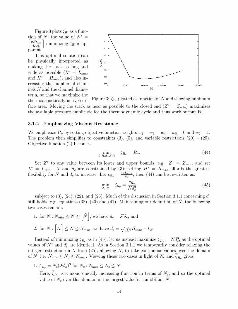
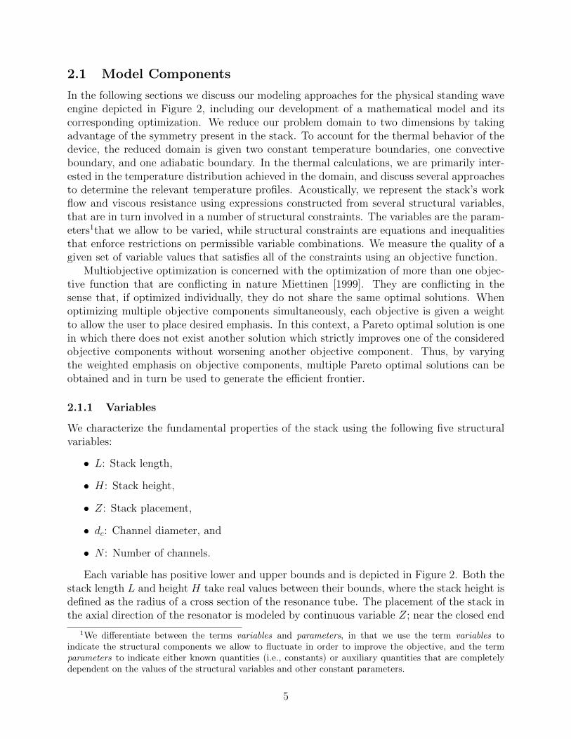
Figure 3: ζW plotted as function of N and showing minimum

Figure 3 plots ζW as a func-tion of N ; the value of N∗ =⌈πH2

max

4At2w

⌉minimizing ζW is ap-

parent.This optimal solution can

be physically interpreted asmaking the stack as long andwide as possible (L∗ = Lmaxand H∗ = Hmax), and also in-creasing the number of chan-nels N and the channel diame-ter dc so that we maximize thethermoacoustically active sur-face area. Moving the stack as near as possible to the closed end (Z∗ = Zmin) maximizesthe available pressure amplitude for the thermodynamic cycle and thus work output W .

3.1.2 Emphasizing Viscous Resistance

We emphasize Rν by setting objective function weights w1 = w3 = w4 = w5 = 0 and w2 = 1.The problem then simplifies to constraints (3), (5), and variable restrictions (20) – (25).Objective function (2) becomes:

minL,H,dc,Z,N

ζRν = Rν . (44)

Set Z∗ to any value between its lower and upper bounds, e.g. Z∗ = Zmin, and setL∗ = Lmin. N and dc are constrained by (3); setting H∗ = Hmax affords the greatestflexibility for N and dc to increase. Let cRν = 4µLmin

δν, then (44) can be rewritten as:

mindc,N

ζRν =cRνNd3c

(45)

subject to (3), (24), (22), and (25). Much of the discussion in Section 3.1.1 concerning dcstill holds, e.g. equations (38), (40) and (41). Maintaining our definition of N , the followingtwo cases remain:

1. for N : Nmin ≤ N ≤⌊N⌋, we have dc = Fδκ, and

2. for N :⌈N⌉≤ N ≤ Nmax, we have dc =

√πANHmax − tw.

Instead of minimizing ζRν as in (45), let us instead maximize ζRν = Nd3c , as the optimalvalues of N∗ and d∗c are identical. As in Section 3.1.1 we temporarily consider relaxing theinteger restriction on N from (25), allowing Nc to take continuous values over the domainof N , i.e. Nmin ≤ Nc ≤ Nmax. Viewing these two cases in light of Nc and ζRν gives:

1. ζRν = Nc(Fδκ)3 for Nc : Nmin ≤ Nc ≤ N .

Here, ζRν is a monotonically increasing function in terms of Nc, and so the optimal

value of Nc over this domain is the largest value it can obtain, N .

14

2. ζRν = Nc

(√πANcHmax − tw

)3for Nc : N ≤ Nc ≤ Nmax.

Over this interval, differentiating ζRν gives:

dζRνdNc

=3t2w2

( πAH2max

) 12N− 1

2c − 1

2

( πAH2max

) 32N− 3

2c − t3w, (46)

and upon a second differentiation, we obtain:

d2ζRνdN2

c

=3

4

( πAH2max

) 32N− 5

2c − 3t2w

4

( πAH2max

) 12N− 3

2c . (47)

The second derivative of ζRν > 0 over the entire domain Nc : N < Nc ≤ Nmax, implying

ζRν is convex. Thus the maximum over this domain occurs at one of the endpoints of

the interval, i.e., N∗c ∈{N ,Nmax

}.

From these two cases, and because N ∈ ZZ+ we have:

N∗ ∈{⌊N⌋,⌈N⌉, Nmax

}; d∗c =

{Fδκ if N∗ =

⌊N⌋

;√πAN∗Hmax − tw otherwise.

(48)

We then choose from (48) the values of N and corresponding dc that minimize (45). Forour specific problem parameters, a global minimizer for ζRν is:

x∗ =[Lmin, Hmax,Fδκ, Zmin,

⌊N⌋].

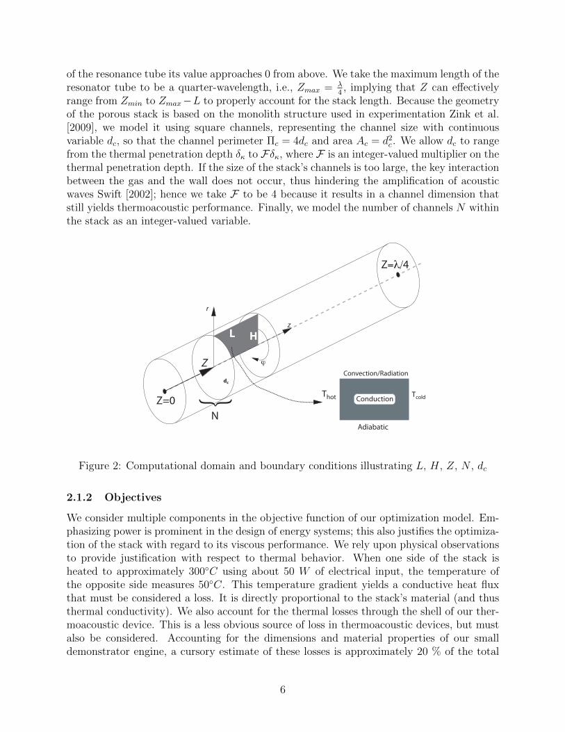
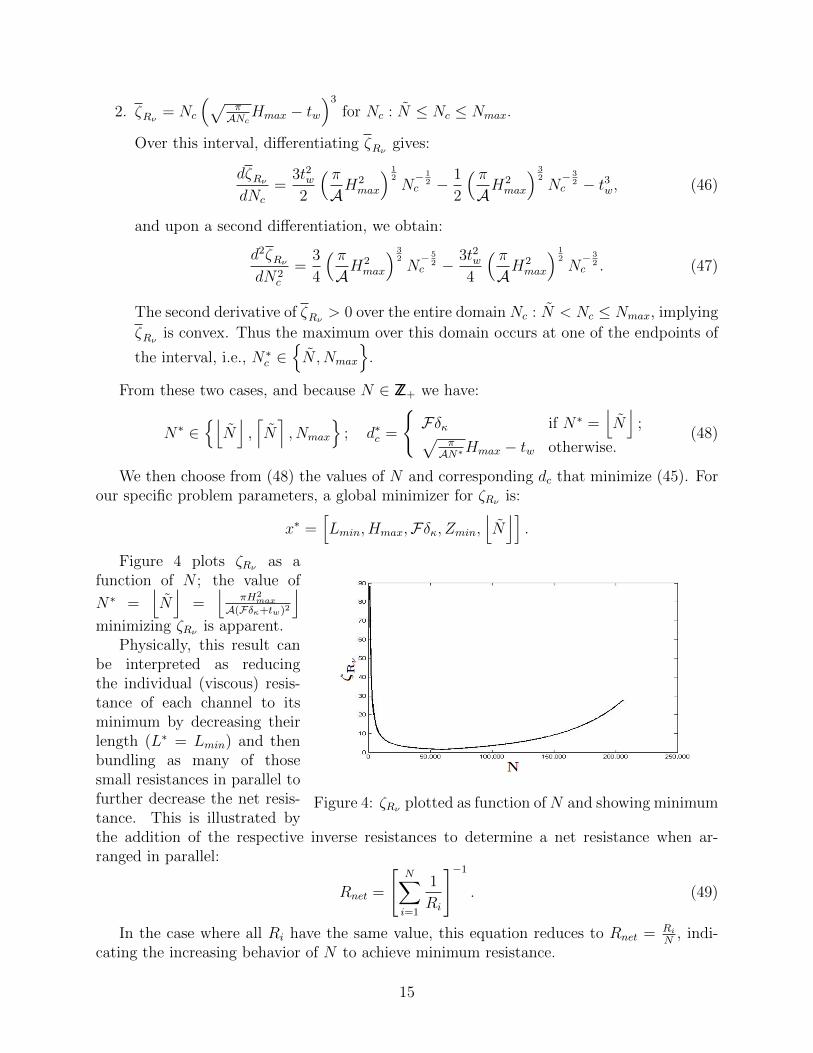
Figure 4: ζRν plotted as function ofN and showing minimum

Figure 4 plots ζRν as afunction of N ; the value of

N∗ =⌊N⌋

=⌊

πH2max

A(Fδκ+tw)2

⌋minimizing ζRν is apparent.

Physically, this result canbe interpreted as reducingthe individual (viscous) resis-tance of each channel to itsminimum by decreasing theirlength (L∗ = Lmin) and thenbundling as many of thosesmall resistances in parallel tofurther decrease the net resis-tance. This is illustrated bythe addition of the respective inverse resistances to determine a net resistance when ar-ranged in parallel:

Rnet =

[N∑i=1

1

Ri

]−1. (49)

In the case where all Ri have the same value, this equation reduces to Rnet = RiN

, indi-cating the increasing behavior of N to achieve minimum resistance.

15

3.2 Thermal Emphasis

We have thus far considered how acoustic objectives W and Rν are affected by changes inthe structural variables. We next discuss the individual thermal objectives by isolating eachheat flow objective function component.

3.2.1 Emphasizing Convective, Radiative Heat Fluxes

We can emphasize Qconv by setting objective function weights w1 = w2 = w4 = w5 = 0 andw3 = 1. The problem then reduces to constraints (3), (10) – (13), variable restrictions (20) –(25), and expression (31). Alternatively, we can emphasize Qrad by setting objective functionweights w1 = w2 = w3 = w5 = 0 and w4 = 1, so that only constraints (3), (16), variablerestrictions (20) – (25), and (32) are active. For these restricted optimization problems,objective function (2) becomes, respectively:

minL,H,dc,Z,N

ζQconv = Qconv; minL,H,dc,Z,N

ζQrad = Qrad. (50)

Neither of these restricted models are dependent on Z, so Z∗ can be set to any valuebetween its lower and upper bounds (note our assumption that h is not dependent on Z inRemark 3). Considering H, for Qcond it can be shown from equations (10) – (13) that h isproportional to H−1/4. Because the resulting exponent on the H variable remains positivein equation (31), it is still desirable to set H∗ = Hmin. For Qrad we also set H to H∗ = Hmin

based on (32). Setting N∗ = Nmin and d∗c = dcmin ensures that H can take its minimumvalue in constraint (3) (see assumption in Remark 4).

A global optimum minimizing both ζQconv and ζQrad is x∗ = [Lmin, Hmin, dcmin , Zmin, Nmin].For Qcond, this optimum minimizes the surface area and limits the temperature range in thestack, thereby minimizing the convective heat flow. Similarly for Qrad, this optimum lowersdriving potential and surface area to minimize radiative heat flow.

3.2.2 Emphasizing Conductive Heat Flux

We emphasize Qcond by setting objective function weights w1 = w2 = w3 = w4 = 0 andw5 = 1, so that only constraints (3), (15), variable restrictions (20) – (25), and (34) areactive. Objective function (2) becomes:

minL,H,dc,Z,N

ζQcond = Qcond. (51)

Similar to previous sections, this model is not dependent on Z, so that Z∗ can be set toany value between its lower and upper bounds. Equation (15) can be rearranged as:

kzz = kg +tw(ks − kg)(tw + dc)

, (52)

and so merging (52) with (34) and rearranging gives:

Qcond = πTc

[kg +

tw(ks − kg)(tw + dc)

]ln (∇TL+ Tc)− ln (Tc)

LH2. (53)

16

The expression ln(∇TL+Tc)−ln(Tc)L

is always positive, so setting L∗ to Lmax decreases Qcond,improving (51). We can also improve Qcond by both decreasing H and increasing dc. How-ever, there is tension in constraint (3) between decreasing H and increasing dc. Because Nappears only on the left-hand side of (3) in this restricted model, we can set N∗ = Nmin = 1

to allow dc and H the most flexibility. Letting cQ1 = πTckgln(∇TLmax+Tc)−ln(Tc)

Lmaxand cQ2 =

πTc [tw(ks − kg)] ln(∇TLmax+Tc)−ln(Tc)Lmax, and noting both are positive, then substituting these

into (53) and (51) gives the following optimization problem over two continuous variables:

minH,dc

ζQcond = cQ1H2 + cQ2

H2

(tw + dc)(54)

subject to constraint (3) and variable restrictions (21), (22), and (25).Given any fixed value for H, it follows from our discussions and (3) that dc will take the

value of:

dc = min

{Fδκ,

√π

AH − tw

}. (55)

Let H = Fδκ+tw√πA

be the value of H for which the value of dc transitions in (55). This

leaves us with two cases:

1. for H : Hmin ≤ H ≤ H, we have dc =√

πAH − tw, and

2. for H : H ≤ H ≤ Hmax, we have dc = Fδκ.

For both intervals ζQcond is nondecreasing, so that H∗ = Hmin, implying d∗c =√

πAHmin−

tw. Thus a global optimum minimizing ζQcond is x∗ =[Lmax, Hmin,

√πAHmin − tw, Zmin, Nmin

].

The physical interpretation of these results indicates that minimizing the conductive heatflow yields a different solution than that of the convective and radiative heat flows. The chan-nel design is a function of gas and solid thermal conductivity, and takes an optimal value be-tween its upper and lower bounds. For an actual engine design this information may be usefulin designing stacks that require the least amount of cooling for a given (heat) power input.

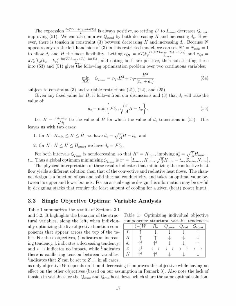
3.3 Single Objective Optima: Variable Analysis

Table 1: Optimizing individual objectivecomponents: structural variable tendencies

(−)W Rν Qconv Qrad Qcond

L ↑ ↓ ↓ ↓ ↑H ↑ ↑ ↓ ↓ ↓dc ↑† ↑† ↓ ↓ ↑Z ↓‡ ←→ ←→ ←→ ←→N ↑† ↑† ↓ ↓ ↓

Table 1 summarizes the results of Sections 3.1and 3.2. It highlights the behavior of the struc-tural variables, along the left, when individu-ally optimizing the five objective function com-ponents that appear across the top of the ta-ble. For these objectives, ↑ indicates an increas-ing tendency, ↓ indicates a decreasing tendency,and ←→ indicates no impact, while †indicatesthere is conflicting tension between variables.‡indicates that Z can be set to Zmin in all cases,as only objective W depends on it, and decreasing it improves this objective while having noeffect on the other objectives (based on our assumption in Remark 3). Also note the lack oftension in variables for the Qconv and Qrad heat flows, which share the same optimal solution.

17

4 Multiobjective Optimization

In Section 3 we examine optimization over every individual component of objective func-tion (2), providing analytical solutions that do not require computational solution methodsto identify global optima. In this section we consider multiple objective components simul-taneously, and suggest straightforward algorithmic approaches to identify optimal solutionsfor these cases. Before proceeding, we first discuss our approach to ensure objective func-tion weights are normalized, which is necessary whenever more than one objective functioncomponent is considered.

4.1 Normalizing Objective Function Components

When multiple objective function components are given nonzero weights, objective func-tion (2) of (MPF) can have a predisposed bias towards those components having largermagnitudes, and unit discrepancies across the various objective components create furthercomplications. These issues can be simultaneously addressed for each objective componentby obtaining a normalization factor to offset any disparate magnitudes and eliminate incon-sistent units.

Our proposed normalization approach is based on a method described in Grodzevichand Romanko [2006]. Let a set I of objective components of interest from objective (2) beindexed by i ∈ I. As (MPF) contains five objective components, |I| ≤ 5. Then for all indicesj /∈ I, we set wj = 0. For normalization coefficients ni the approach uses the differencesof values between certain Utopia and Nadir vectors that are of the same dimension as thenumber of considered objective function components |I|, and are formed using informationobtained from independent optimization of each objective function component.

The Utopia vector U is created as follows. For each i ∈ I, we set wi = 1 and wk =0 ∀ k ∈ I : k 6= i. Let Gi be the selected objective component. Optimizing the resultingreduced problem generates optimal objective function value G∗i and optimal solution x∗i =[L∗i , H

∗i , d

∗ci, Z∗i , N

∗i ]. Then Ui = G∗i . After repeating this process for all i ∈ I, the Nadir

vector N makes use of the optimal solutions x∗i from these optimizations, evaluating eachx∗i in the respective individual objective functions G∗i over all i ∈ I to find its worst value.Thus, the Nadir vector is constructed as Ni = max

`=1,...,5{Gi(x∗`)} ∀ i ∈ I.

For each i ∈ I, the differencesNi−Ui provide the length of interval over which the optimalobjective functions vary within the set of optimal solutions; note that these differences arealways non-negative. They are used to construct the normalization factors ni as:

ni =1

Ni − Ui. (56)

For instance, if we consider for I all five of the objective components of objective func-tion (2), then it can be normalized as:

w1n1((−W )−U1)+w2n2(Rν−U2)+w3n3(Qconv−U3)+w4n4(Qrad−U4)+w5n5(Qcond−U5).(57)

We use this normalization scheme for all cases involving multiple objective function com-ponents. Note that the Utopia values are subtracted from every component so to ensurethat the term is unitless and nonnegative, thereby eliminating any bias of magnitude.

18

4.2 Emphasizing Work and Viscous Resistance

We can simultaneously optimize the acoustic objectives W and Rν by assigning objec-tive weights w3 = w4 = w5 = 0 with w1 > 0, w2 > 0. Then (MPF) reduces to con-straints (3), (4), (17) – (19) and variable restrictions (20) – (25). Objective function (2)reduces to:

minL,H,dc,Z,N

ζAcoustic = w1(−W ) + w2Rν . (58)

With respect to (36), let cW = −w1fW (Zmin) and cRν = w24µδν

, so that cW and cRν are,respectively, the constant terms from Sections 3.1.1 and 3.1.2 without fixing L. SettingZ∗ = Zmin and H∗ = Hmax as in Sections 3.1.1 and 3.1.2, and substituting cW , cRν , W andRν into objective function (58) gives:

minL,N,dc

ζAcoustic =

(cWNdc +

cRνNd3c

)L (59)

subject to (20), (24), (22), (25), and (38). The tradeoffs between variables L, N and dccan be investigated by first fixingN toN ∈ [Nmin, Nmax]∩ZZ, then usingN in equation (40) to

fix dc to dc = min{Fδκ,

√πANHmax − tw

}. Depending on the sign of the resulting coefficient

on L in (59), L can be set to:

L =

{Lmin if

(cWN dc +

cRν

N dc3

)≥ 0;

Lmax otherwise.(60)

Figure 5: Simultaneously minimizing −W and Rν

Thus for every fixed N the prob-lem has a fixed value of dc and L. Theoptimal levels of L∗, N∗ and d∗c can befound by enumerating over all valuesN ∈ [Nmin, Nmax]∩ZZ. We implementsuch an approach in MATLAB Mat[2007], which takes at most a few min-utes to solve on a Windows XP ma-chine equipped with a 2.16GHz IntelCore 2 processor and 2GB of RAM.

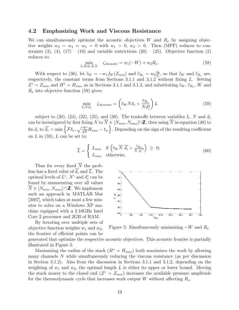
By iterating over multiple sets ofobjective function weights w1 and w2,the frontier of efficient points can begenerated that optimize the respective acoustic objectives. This acoustic frontier is partiallyillustrated in Figure 5.

Maximizing the radius of the stack (H∗ = Hmax) both maximizes the work by allowingmany channels N while simultaneously reducing the viscous resistance (as per discussionin Section 3.1.2). Also from the discussion in Sections 3.1.1 and 3.1.2, depending on theweighting of w1 and w2, the optimal length L is either its upper or lower bound. Movingthe stack nearer to the closed end (Z∗ = Zmin) increases the available pressure amplitudefor the thermodynamic cycle that increases work output W without affecting Rν .

19

4.3 Emphasizing All Objective Components

Lastly, we simultaneously consider all five objective components by regarding work W andviscous resistance Rν as two distinct objective components, and representing heat with athird distinct objective component Qall, defined as the sum of the three heat componentsQconv, Qrad, and Qcond. We use three weights, wW , wRν and wQall , and divide wQall equallyamong the three heat components comprising Qall.

As in Section 4.2, we propose to determine the frontier of efficient points that optimizethe three weighted objectives W , Rν , and Qall by iterating over multiple values of objectivefunction weights wW , wRν and wQall . However, due to the lack of a closed form solution overthe considered objective function components, this requires a global optimization approachto identify optimal solutions.

For fixed values of wW , wRν and wQall , we call the global optimization routine DI-RECT Perttunen et al. [1993], a derivative free algorithm based on Lipschitzian optimizationwith proven finite convergence. The algorithm begins by constructing a hyper-rectangle thatcontains the original (continuous) variable space, and progressively improves the objectiveby repeatedly sub-dividing hyper-rectangles as it moves toward the global optimum. Theparticular implementation we use is due to Finkel Finkel [2003], and coded in MATLAB.

This process generates optimal solutions corresponding to various sets of weights wW ,wRν and wQall . These optimal solutions are then used to construct the efficient frontier ofoptimal solutions, which is partially illustrated in the three-dimensional objective space bythe fitted surface appearing in Figures 6(a) and 6(b). The conflicting nature of the threeobjectives can be observed in both profiles, with each competing objective on respective axes.Figure 6(a) provides a side profile of the efficient frontier, where the bottom left corner isimproving for all three objectives, and illustrates how an improvement in a single objectivecomponent causes the remaining two objectives to worsen. Figure 6(b) depicts the samephenomenon from a top profile, where the rear corner is improving for every objective.

5 Conclusions

We demonstrate how optimization techniques can improve the design of thermoacoustic de-vices. Previous studies have largely relied upon parametric studies. In contrast to these,where only one parameter is varied while all others are kept constant, we propose a math-ematical model that simultaneously optimizes multiple variables over a set of constraints,and includes an objective function quantifying both acoustic and thermal performance.

We analyze cases of single objective components (two acoustic and three thermal), aswell as two cases of multiobjective optimization. For the single objective cases, we identifyanalytical solutions, while for the cases of multiple objectives, we generate the efficientfrontier of optimal solutions for various objective weights. For both cases (the single objectiveas well as multiple objective approach), we show that there are non-trivial solutions toeach design that have the potential to improve the energetic performance of thermoacousticdevices. The approach presented here still allows for a large amount of personal preference,i.e. emphasis on purely acoustic performance or purely thermal performance, or any givenblend of the two main groups of objectives.

20

An alternative way to simultaneously maximize work and minimize losses (viscous re-sistance as well as heat flows) is to consider the thermal efficiency η, which can be definedas the ratio of the work output over the sum of the work output and losses. Thus we canconsider the following optimization problem:

maxW

W + w2Rv + w3Qconv + w4Qrad + w5Qcond

(61)

subject to the original constraints of (MPF). This results in a mixed-integer fractionalprogramming problem, the numerator of which represents the work output, and the denom-inator being a sum of the work and combined (viscous and thermal) losses.

One way to solve fractional programs is via Dinkelbach’s algorithm Dinkelbach [1967].Briefly, Dinkelbach’s algorithm eliminates the ratio in objective (61) by instead consideringa sequence of problems that parameterize (61) with:

η =W

W + w2Rv + w3Qconv + w4Qrad + w5Qcond

, (62)

and replace objective function (61) by:

max W − η(W + w2Rv + w3Qconv + w4Qrad + w5Qcond). (63)

Dinkelbach’s algorithm optimizes (63) subject to the original (MPF) constraints, itera-tively updating its choice of η in order to identify η∗ for which the maximum value of (63)equals zero. The sequence of choices for η finitely converge to η∗, solving the alternative rep-resentation and thus the original problem as well. Note the equivalence between the versionof (MPF) as described in Section 4.3, and that of a single instance of (63) (correspondingto a fixed value of η) subject to the constraints in (MPF). Therefore solving (61) can bereduced to iteratively applying our procedure until the maximum of (63) attains zero.

6 Acknowledgements

The authors thank two anonymous referees whose constructive comments substantially im-proved this manuscript. Andrew C. Trapp was supported by the US Department of Educa-tion Graduate Assistance in Areas of National Need (GAANN) Fellowship Program grantP200A060149, administered through the Mascaro Center for Sustainable Innovation at theUniversity of Pittsburgh. Laura Schaefer was supported by NSF grant CBET-0729905.

21

7 Nomenclature

A Area (m2)c Speed of sound (m · s−1)C Capacitance (m−1)cp Heat capacity (J · kg−1 ·K−1)d DiameterD Dimensionf Frequency (s−1)g Gravitational accelerationh Heat transfer coefficient (W ·m−2 ·K−1)H Height (Cylindrical Radius) (m)kb Boltzmann constantk Thermal conductivity (W ·m−1 ·K−1)l Plate thickness (m)L Inertance (kg ·m−4), length (m)p Pressure (N ·m−2)p Constant for quadratic pressure estimateQ Heat flow (W)r Variable radius height (m) along radial directionr Constant for viscous resistance formulationR Resistance (kg ·m−2 · s−1)T Temperature (K, ◦C)u Velocity (m · s−1)u Constant for quadratic velocity estimatew Objective function component weightW Acoustic work (W) per channely Plate spacing (m)z Local variable, refers to distance along the stack, 0 at “hot side” of

stackZ Stack Placement (along z axis), 0 at closed end

22

Greek Symbols

α Thermal diffusion rate (m2 · s−1)β Thermal expansion coefficient (taken as

1/T∞)δ Penetration depth (m)ε Plate heat capacity ratioε Surface emissivityγ Isentropic coefficientΓ Temperature gradient ratioλ Wavelengthµ Dynamic viscosity (kg ·m−1 · s−1)ν Viscous diffusion rate (m2 · s−1)ρ Density (kg ·m−3)ω Angular frequency (s−1)Π Perimeter (m)∇T Temperature gradient (K ·m−1)

Dimensionless Groups

A Packing Number (≈ 1.25± 0.25)F Fixed Upper Bounding Constant

(4)Gr Grasshoff NumberNu Nusselt NumberPr Prandtl NumberRa Rayleigh Number

23

Subscripts and Superscripts

o Naught∞ Ambient, free streamc Channel, coldchar Characteristiccrit Criticalcond Conductiveconv ConvectiveD Diameterh Hot sideκ Thermalm Time averagedobj Objectiverad Radiatives Solid, surface, stablerr,rz,zr,zz Tensor directionsν Viscousw Wall

References

Scott Backhaus and Greg W. Swift. A thermoacoustic Stirling heat engine: Detailed study.Journal of the Acoustical Society of America, 107(6):3148–66, 2000.

Kevin J. Bastyr and Robert M. Keolian. High-frequency thermoacoustic-Stirling heat enginedemonstration device. Acoustics Research Letters Online, 4(2):37–40, 2003.

Etienne Besnoin. Numerical Study of Thermoacoustic Heat Exchangers. PhD thesis, JohnsHopkins University, 2001.

Peter H. Ceperley. Gain and efficiency of a short traveling wave heat engine. Journal of theAcoustical Society of America, 77(3):1239–1244, 1985.

Comsol Multiphysics Users Guide. COMSOL AB, Burlington, MA, USA, 2005.

W. Dinkelbach. On non-linear fractional programming. Management Science, 13(7):492–498,1967.

Daniel E. Finkel. DIRECT Optimization Algorithm User Guide. Center for Research inScientific Computation, North Carolina State University, Raleigh, NC 27695-8205, March2003.

Erich Friedman. http://www2.stetson.edu/˜efriedma/squincir/.

Steven L. Garrett. Reinventing the engine. Nature, 339:303–305, 1999.

Steven L. Garrett. The power of sound. American Scientist, 88(6):516–526, 2000.

24

O. Grodzevich and O. Romanko. Normalization and other topics in multiobjective op-timization. In Proceedings of the First Fields-MITACS Industrial Problems Workshop,pages 89–102. The Fields Institute, 2006.

Cila Herman and Z Travnicek. Cool sound: The future of refrigeration? Thermodynamicand heat transfer issues in thermoacoustic refrigeration. Heat and Mass Transfer, 42:492–500, 2006.

Noboru Kagawa. Regenerative Thermal Machines. International Institute for Refrigeration,Paris, 2000.

S C. Kaushik and S Kumar. Finite time thermodynamic analysis of endoreversible Stirlingheat engine with regenerative losses. Energy, 25:989–1003, 2000.

MATLAB User’s Guide. The MathWorks, Inc., 2007.

K. Miettinen. Nonlinear multiobjective optimization. Springer, 1999.

Brian L. Minner, James E. Braun, and Luc G. Mongeau. Theoretical evaluation of the opti-mal performance of a thermoacoustic refrigerator. In ASHRAE Transactions: Symposia,volume 103, pages 873–887, 1997.

C. D. Perttunen, D. R. Jones, and B. E. Stuckman. Lipschitzian optimization without thelipschitz constant. Journal of Optimization Theory and Application, 79(1):157–181, 1993.

Matthew E. Poese, Robert W.M. Smith, Steven L. Garrett, Rene van Gerwen, and PeteGosselin. Thermoacoustic refrigeration for ice cream sales. In Proceedings of the 6th IIRGustav Lorentzen Conference, 2004.

Greg W. Swift. Thermoacoustic engines. Journal of the Acoustical Society of America, 84(4):1145–1180, 1988.

Greg W. Swift. Thermoacoustics: A unifying perspective for some engines and refrigerators.Acoustical Society of America, Melville NY, 2002.

Gregory W. Swift, Scott N. Backhaus, and David L. Gardner. Us pat. no. 6032464, 2000.

K Tang, R Bao, G B. Chen, Y Qiu, L Shou, Z J. Huang, and T Jin. Thermoacousticallydriven pulse tube cooler below 60 K. Cryogenics, 47:526–529, 2007.

M E. H. Tijani, J C. H. Zeegers, and A T. A. M. de Waele. Design of thermoacousticrefrigerators. Cryogenics, 42:49–57, 2002.

Y Ueda, T Biwa, U Mizutani, and T Yazaki. Experimental studies of a thermoacousticStirling prime mover and its application to a cooler. Journal of the Acoustical Society ofAmerica, 72(3):1134–1141, 2003.

Srinivas Vanapalli, Michael Lewis, Zhihua Gan, and Ray Radebaugh. 120 Hz pulse tubecryocooler for fast cooldown to 50 K. Applied Physics Letter, 90, 2007.

25

Martin Wetzel. Experimental Investigation of a Single Plate Thermoacoustic Refrigerators.PhD thesis, Johns Hopkins University, 1998.

J H. Xiao. Thermoacoustic heat transportation and energy transformation, part 3: Adiabaticwall thermoacoustic effects. Cryogenics, 35(1):27–29, 1995.

F. Zink, H. Waterer, R. Archer, and L. Schaefer. Geometric optimization of a thermoacousticregenerator. International Journal of Thermal Sciences, 48:2309–2322, 2009.

Luke Zoontjens, Carl Q. Howard, Anthony C. Zander, and Ben S. Cazzolato. Modelling andoptimisation of acoustic inertance segments for thermoacoustic devices. In Proceedings ofACOUSTICS 2006, pages 435–441, 2006.

26

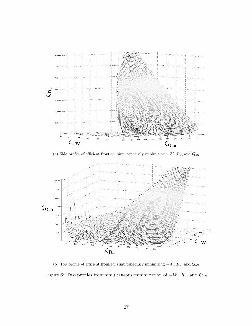
(a) Side profile of efficient frontier: simultaneously minimizing −W , Rν , and Qall

(b) Top profile of efficient frontier: simultaneously minimizing −W , Rν , and Qall

Figure 6: Two profiles from simultaneous minimization of −W , Rν , and Qall

27