Embed Size (px)
Citation preview
NASA / CR--2000-210055
Thermophysical Properties of GRCop-84
David L. Ellis
Case Western Reserve University, Cleveland, Ohio
Dennis J. Keller
RealWorld Quality Systems, Inc., Cleveland, Ohio
June 2000

The NASA STI Program Office... in Profile
Since its founding, NASA has been dedicated tothe advancement of aeronautics and spacescience. The NASA Scientific and Technical
Information (STI) Program Office plays a key part
in helping NASA maintain this important role.
The NASA STI Program Office is operated by
Langley Research Center, the Lead Center forNASA's scientific and technical information. The
NASA STI Program Office provides access to the
NASA STI Database, the largest collection ofaeronautical and space science STI in the world.
The Program Office is also NASA's institutional
mechanism for disseminating the results of itsresearch and development activities. These results
are published by NASA in the NASA STI Report
Series, which includes the following report types:
TECHNICAL PUBLICATION. Reports ofcompleted research or a major significant
phase of research that present the results ofNASA programs and include extensive data
or theoretical analysis. Includes compilations
of significant scientific and technical data andinformation deemed to be of continuing
reference value. NASA's counterpart of peer-reviewed formal professional papers but
has less stringent limitations on manuscript
length and extent of graphic presentations.
TECHNICAL MEMORANDUM. Scientific
and technical findings that are preliminary or
of specialized interest, e.g., quick release
reports, working papers, and bibliographiesthat contain minimal annotation. Does not
contain extensive analysis.
CONTRACTOR REPORT. Scientific and
technical findings by NASA-sponsoredcontractors and grantees.
CONFERENCE PUBLICATION. Collected
papers from scientific and technical
conferences, symposia, seminars, or othermeetings sponsored or cosponsored byNASA.
SPECIAL PUBLICATION. Scientific,
technical, or historical information from
NASA programs, projects, and missions,often concerned with subjects having
substantial public interest.
TECHNICAL TRANSLATION. English-language translations of foreign scientific
and technical material pertinent to NASA'smission.
Specialized services that complement the STIProgram Office's diverse offerings include
creating custom thesauri, building customized
data bases, organizing and publishing researchresults.., even providing videos.
For more information about the NASA STI
Program Office, see the following:
• Access the NASA STI Program Home Page
at http://www.sti.nasa.gov
• E-mail your question via the Internet [email protected]
• Fax your question to the NASA AccessHelp Desk at (301) 621-0134
• Telephone the NASA Access Help Desk at(301) 621-0390
Write to:
NASA Access Help Desk
NASA Center for AeroSpace Information7121 Standard Drive
Hanover, MD 21076
NASA/CR--2000-210055
Thermophysical Properties of GRCop-84
David L. Ellis
Case Western Reserve University, Cleveland, Ohio
Dennis J. Keller
RealWorld Quality Systems, Inc., Cleveland, Ohio
Prepared under Contract NAS3-463
National Aeronautics and
Space Administration
Glenn Research Center
June 2000
Acknowledgments
The authors would like to thank Raymond Taylor and the staff at TPRL, Inc. for conducting much of the
thermophysical testing, answering questions regarding the testing and providing insight into the results.The authors would also like to thank Patrick M. Martin of ORNL for conducting the low temperature
electrical resistivity measurements.
Trade names or manufacturers' names are used in this report for
identification only: This usage does not constitute an official
endorsement, either expressed or implied, by the National
Aeronautics and Space Administration.
NASA Center for Aerospace Information7121 Standard Drive
Hanover, MD 21076Price Code: A03
Available from
National Technical Information Service
5285 Port Royal Road
Springfield, VA 22100Price Code: A03
Thermophysical Properties Of GRCop-84
David L. Ellis
Case Western Reserve UniversityCleveland, OH 44106-7204
Dennis J. Keller
RealWorld Quality Systems, Inc.Cleveland, OH 44116
AbstractThe thermophysical properties and electrical resistivity of GRCop-84 (Cu - 8 at.% Cr-4 at.% Nb) were
measured from cryogenic temperatures to near its melting point. The data were analyzed using weighted regressionto determine the properties as a function of temperature and assign appropriate confidence intervals.
The results showed that the thermal expansion of GRCop-84 was significantly lower than NARIoy-Z(Cu-3 wt.% Ag-0.5 wt.% Zr), the currently used thrust cell liner material. The lower thermal expansion is expected
to translate into lower thermally induced stresses and increases in thrust cell liner lives between 2X and 4IX over
NARloy-Z. The somewhat lower thermal conductivity of GRCop-84 can be offset by redesigning the liners toutilize its much greater mechanical properties. Optimized designs are not expected to suffer from the lower thermal
conductivity. Electrical resistivity data, while not central to the primary application, show that GRCop-84 haspotential for applications where a combination of good electrical conductivity and strength is required.
Introduction
New ternary Cu-Cr-Nb alloys are under consideration for use in several high heat flux, high temperatureapplications such as combustion chamber liners for regeneratively cooled rocket engines. One alloy, GRCop-84
(Cu - 8 at.% Cr - 4 at.% Nb) has been selected for further development in the Reusable Launch Vehicle (RLV)
program. As part of the design of the engines, it is necessary to determine the mechanical and thermophysicalproperties of GRCop-84 over the potential operating conditions. This portion of the effort experimentally measured
the thermal conductivity and thermal expansion of GRCop-84 from cryogenic temperatures to near the melting pointof the alloy and assigned confidence intervals on those measurements.
NARIoy-Z (Cu-3 wt.% Ag-0.5 wt.% Zr) is currently used for the space shuttle main engine (SSME).NARloy-Z possesses very high thermal conductivity, but suffers from lower than desired elevated temperaturemechanical properties. GRCop-84 has shown considerably better mechanical properties (1 - 3) but a lower thermal
conductivity. As part of the trade studies required for the alloy selections and design of the engines, the benefits ofincreased mechanical and other properties will be weighed against the lower thermal conductivity. NARIoy-Z is
also 5% denser than GRCop-84. For the RLV program where the design could call for hundreds of small thrustcells, the lower density can translate into lower engine weight, increased thrust-to-weight ratio and larger payloads.
Experimental Procedure
Alloy Production
Five separate powder production runs or lots of GRCop-84 were made at Crucible Research in Pittsburgh,PA. Each powder lot was kept separate during production and consolidation so they represent true statistical
repeats. Each powder lot was canned in three t5.2 cm (6 inch) diameter mild steel extrusion cans by CrucibleResearch and delivered to CSM Industries in Coldwater, MI for extrusion. Each can was extruded using a reduction
in area ratio of 29.5, which resulted in a total of 15 extruded bars with an average diameter of 2.8 cm (1.1 inches)and an average length of 3.96 m (13 feet). One sample was taken from each extrusion for each type of testing.
Therrnophysical Testing
Because of the need for specialized equipment, most of the thermophysical testing was conducted at TPRLInc. in West Lafayette, IN. Elevated temperature thermal expansion testing was conducted at the NASA Glenn
Research Center in Cleveland, OH, to complete the database.
NASA/CR--2000-210055 1
Thermal Conductivity
Thermal conductivity was measured and calculated by various methods from 30 K (-405°F) to 1173 K
(1652°F).For testing at room temperature and above, the laser flash technique was employed. This technique
requires the measurement of the room temperature bulk density (PRT), the specific heat (ce) and the thermal
diffusivity (_). The room temperature bulk density was measured using a Micromeritics AccuPyc 1330 pycnometerand an Ainsworth AA-160 digital balance. The specific heat was measured using a Perkin-Elmers Model DSC-2Differential Scanning Calorimeter (DSC) from room temperature to 573 K (572°F). Between 573 K and 1173 K
and below room temperature, a Netzsch Model 404 DSC was used to measure the specific heat. Both DSCs used a
sapphire standard. Thermal diffusivity was determined by heating a specimen to the desired temperature andsubjecting the front face of the sample to a short laser burst. By monitoring the small rise in temperature of the backside with time and knowing the thickness of the sample, the thermal diffusivity can be calculated. The thermal
conductivity (_,) at temperature T was then calculated using (4)
X(T) = ct(T) ce(T) PRr [1]
For thermal conductivity testing from below room temperature to about 473 K, the Kohlrausch method (5)
was used. The sample was resistively heated by passing a direct current through the sample while the ends were
kept at a constant temperature. This establishes a thermal gradient along the length of the sample which is measuredby thermocouples placed at the center of the specimen and 1.0 cm (0.39 inches) to both sides of the center. Inaddition, the two outer thermocouples are also used as voltage probes to measure the voltage drop across the
specimen. To minimize radial heat loss, the sample is surrounded by a heater that is maintained at the temperatureof the center thermocoupte. When steady state is achieved, the axial temperature distribution is a parabola.
The product of the thermal conductivity and electrical resistivity at any temperature can be calculated from
;_(_)o(T2) - (V_-V,) 2 [2]412T2 -(T t +7"3)]
where V_-V_ is the voltage drop measured by the outer thermocouples, T2 is the center temperature, and Tz and Tj arethe outer temperatures. The resistivity of the specimens can be calculated knowing the cross-sectional area (A) and
the current passing through the specimen (/) using the equation
19=(V 3-V I) A [31I l
where I is equal to the 2 cm distance between the thermocouples. After achieving steady state, all values needed aremeasured and the current through the sample increased to increase the temperature for the next measurement.
Low Temperature Electrical ResistivityTPRL Inc. sent one specimen from powder lot 3C to the Superconductor Group at Oak Ridge National
Laboratory (ORNL) for low temperature electrical resistivity testing. The resistivity of the sample was determinedusing the four point resistance method. A current between 1 and 40 mA was supplied by an HP 3245 Universal V/Isource at 27 Hz. The voltage drop across the sample was read by a Par 5209 Lock-in Amplifier. To measure the
temperature, a diode was placed on the sample between the voltage probes. A Lake Shore 330 TemperatureController was used to record the temperature. The sample was cooled in vacuum using a CVI model CGR 409
UHV closed cycle refrigerator. After cooling to 30 K or lower, data were recorded during the warming of the
sample back to room temperature.
Thermal ExpansionPush rod dilatometers were used to measure the thermal expansion of the specimens. The sample is placed
in a holder with a rod pushing against one end of the specimen. As the specimen is heated or cooled, the change in
length of the specimen is measured by a linear variable differential transformer (LVDT) attached to the opposite end
of the push rod. Software compensates for the thermal expansion of the holder and push rod. A thermocouple inintimate contact with the specimen is used to record the temperature. Cryogenic thermal expansion testing was done
at TPRL Inc. Elevated temperature testing was done at NASA GRC using an Orton model 1600C dilatometer. To
protect the specimens from oxidation at elevated temperatures, the holder was enclosed in a furnace tube and He
flowed through the assembly. The results were recorded at 1 K (I.8°F) intervals for the elevated temperature tests
and at approximately 10 K (18°F) intervals for the cryogenic tests.
NAS A/CR--2000-210055 2
Results
Alloy Chemistries
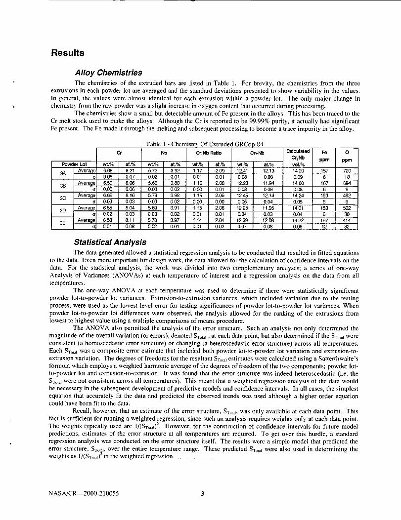
The chemistries of the extruded bars are listed in Table 1. For brevity, the chemistries from the three
extrusions in each powder lot are averaged and the standard deviations presented to show variability in the values.
In general, the values were almost identical for each extrusion within a powder lot. The only major change in
chemistry from the raw powder was a slight increase in oxygen content that occurred during processing.
The chemistries show a small but detectable amount of Fe present in the alloys. This has been traced to the
Cr melt stock used to make the alloys. Although the Cr is reported to be 99.99% purity, it actually had significant
Fe present. The Fe made it through the melting and subsequent processing to become a trace impurity in the alloy.
Powder Lot
3A
3B
3C
3D
3E
Cr
wt.% at.%
Average 6.68 8.21a 0.08 0.07
Average 6.59 8.06a 0.08 0.06
Avera_le, 6.66 8.16a: 0.03 0.03
Average 6.55 8.04
a I 0.02 0.03Averagel 6.58 8.11
_1 0.01 0.08
Table 1 - Chemistry Of Extruded GRCop-84
Nb Cr:Nb Ratio Cr+Nb
wt.% at.%
5.72 3.92
0.02 0.01
5.68 3.88
0.03 0.02
5.79 3.98
0.03 0.02
5.69 3.91
0.03 0.02
5.78 3.97
O.02 0.01
wt.% I at.%
117 I 2090.01 0.01
1,16 2.08
0.00 0.01
1.15 2.05
0.00 0.03
1.15 2.06
0.01 0.01
1.14 2.04
O.OllO.O2
wt.%
12.41
0.08
12.23
0.08
12.45
0.05
12.25
0.04
12.39
0.07
Calculated
Cr=l_
at.% vol.%
12.13 14.20
0.08 0.09
11.94 14.00
0.08 0.08
12.14 t4.24
0.04 0.05
11.95 14.01
0.03 0.04
12.08 14.22
0.08 0.06
Fe 0
ppm ppm
157 720
6 18
167 694
6 9
193 492
6 9
153 562
6 3O
167 414
12 32
Statistical Analysis
The data generated allowed a statistical regression analysis to be conducted that resulted in fitted equations
to the data. Even more important for design work, the data allowed for the calculation of confidence intervals on the
data. For the statistical analysis, the work was divided into two complementary analyses; a series of one-way
Analysis of Variances (ANOVAs) at each temperature of interest and a regression analysis on the data from all
temperatures.
The one-way ANOVA at each temperature was used to determine if there were statistically significant
powder lot-to-powder lot variances. Extrusion-to-extrusion variances, which included variation due to the testing
process, were used as the lowest level error for testing significances of powder lot-to-powder lot variances. When
powder lot-to-powder lot differences were observed, the analysis allowed for the ranking of the extrusions from
lowest to highest value using a multiple comparisons of means procedure.
The ANOVA also permitted the analysis of the error structure. Such an analysis not only determined the
magnitude of the overall variation (or errors), denoted STotal. at each data point, but also determined if the STota I were
consistent (a homoscedastic error structure) or changing (a heteroscedastic error structure) across all temperatures.
Each STo,aj was a composite error estimate that included both powder lot-to-powder lot variation and extrusion-to-
extrusion variation. The degrees of freedoms for the resultant STo,,I estimates were calculated using a Satterthwaite's
formula which employs a weighted harmonic average of the degrees of freedom of the two components; powder lot-
to-powder lot and extrusion-to-extrusion. It was found that the error structure was indeed heteroscedastic (i.e. the
STo,_ were not consistent across all temperatures). This meant that a weighted regression analysis of the data would
be necessary in the subsequent development of predictive models and confidence intervals. In all cases, the simplest
equation that accurately fit the data and predicted the observed trends was used although a higher order equation
could have been fit to the data.
Recall, however, that an estimate of the error structure, STo,,_, was only available at each data point. This
fact is sufficient for running a weighted regression, since such an analysis requires weights only at each data point.
The weights typically used are 1/(STo,_) 2. However, for the construction of confidence intervals for future model
predictions, estimates of the error structure at all temperatures are required. To get over this hurdle, a standard
regression analysis was conducted on the error structure itself. The results were a simple model that predicted the
error structure, STotal, over the entire temperature range. These predicted STota I were also used in determining the
weights as I/(STo,,I) 2 in the weighted regression.
NAS A/CR--2000-210055 3
where
An approximate (1- (z)100% confidence interval on future model predictions is given by the formula
Yc, (T) = f(T) + t(1 - oq v) Sy. x (T) [4]
Yci(T) = the approximate (1- ¢x)100% confidence interval for a future model prediction for property Y at
temperature Tf(T) = the resultant regression equation for prediction of the property Y from temperature T
t(l-_,v) = t value for a given confidence (1-o0 and degrees of freedom (v)Sy.x(T) = the standard error of the regression which is typically estimated under the assumption of
homoscedastic errors as
where N = number of data points and P = number of parameters being estimated
The standard error of the regression, S¥.x, is a measure of goodness of fit of the model to the data. It is
made up of two components: pure error and lack-of-fit (LOF). The pure error component was already estimated inS.o,_l and was found to be heteroscedastic. Hence, Sy.x could not be estimated in the usual way, but had to be
manufactured from Svot_ and an estimate of the LOF component. The LOF component is typically a measurementof the deviation of the mean of the property Y repeats from the model predicted value or in equation form
SL,,_ = I "_ (Y"'""°'K__ Y'"_''¢'_ y [61
where K is the number of means or the number of unique temperatures. Finally, an estimate of Sy.x that captured
the heteroscedastic nature of the error structure was constructed using
s_, (r) =,,/sLr +SL.,,O-) [7]
Hence, the approximate (1-c0100% confidence intervals on future model predictions was calculated according to
Equations 4 and 7.
Thermal Diffusivity
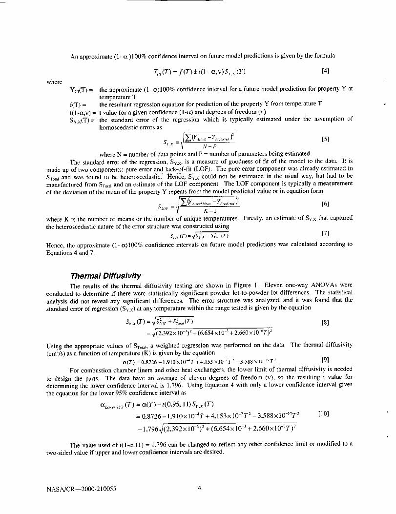
The results of the thermal diffusivity testing are shown in Figure 1. Eleven one-way ANOVAs wereconducted to determine if there were statistically significant powder lot-to-powder lot differences. The statistical
analysis did not reveal any significant differences. The error structure was analyzed, and it was found that thestandard error of regression (Sy.x) at any temperature within the range tested is given by the equation
S,.x (T) = _/S_oF + SL,.:(T) [8]
= _/(2.392 x 10-3) 2+ (6.654 x 10 -3 + 2.660 x 10⁻⁶T) -"
Using the appropriate values of STot_J, a weighted regression was performed on the data. The thermal diffusivity
(cm2/s) as a function of temperature (K) is given by the equation
o_(T) = 0.8726 - 1.910 x 10-_T + 4.153 x 10 -7T 2_ 3.588 x 10_'°T 3 [9]
For combustion chamber liners and other heat exchangers, the lower limit of thermal diffusivity is needed
to design the parts. The data have an average of eleven degrees of freedom (v), so the resulting t value for
determining the lower confidence interval is 1.796. Using Equation 4 with only a lower confidence interval gives
the equation for the lower 95% confidence interval as
aLo,_, 95_¢(T) = or(T) - t(0.95, 11) S, .x (T)
= 0.8726_ 1.910x 10⁻⁴T + 4.153x 10-TT,- _3.588x10-10T3 [10]
- 1.7964(2.392 x 10⁻³) 2 + (6.654 × 10--_+ 2.660x 10⁻⁶T) z
The value used of t(l-cx, l I) = 1.796 can be changed to reflect any other confidence limit or modified to a
two-sided value if upper and lower confidence intervals are desired.
NAS A/CR--2000-210055 4
tot%l
Eo
V
.>_to
t'rJE
t.-.I---
_ - _ _'_"_'"_"¢ ......... _........ .l_.,,..r_.__.,____r._,,_...._. _ ....
0.90 T T-'-°'-'-''_ "-'--'-_''-'_ " "- "
0.85
...... .........................................0.75 ......................................................: ::::::: '.....:_f_ ............
0.70 .......... l Powder LoI3A .................: ..............^,-Lower _0_/o / -\\
• Powder Lot 3B Confidence Interval ".\[] Powder Lot 3C - - ..............\_
0.65 ........._ .....Powder Lot3D ....................:........................................................._,• Powder Lot3E
0.60 .... I .... ,_'-_' I .... I .... I ' ' '
200 400 600 800 1 000 1 200
Temperature (K)
Figure 1 - Thermal Piffusivity Of GRCop-84
I
1400
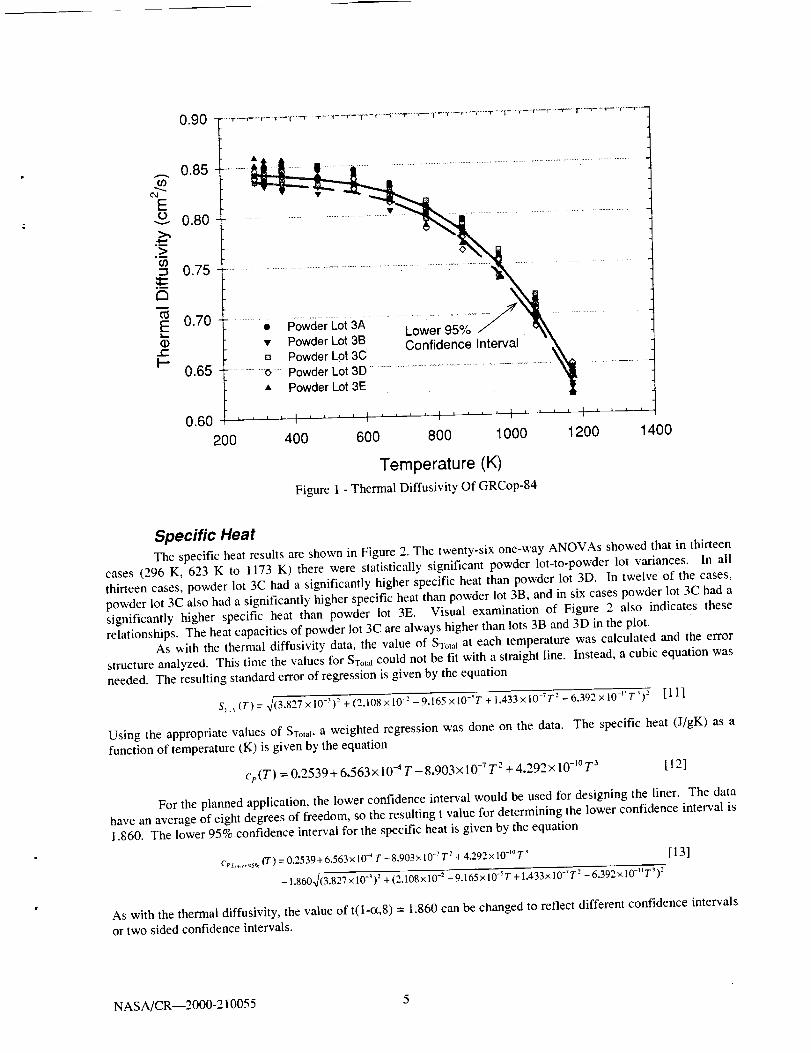
Specific HeatThe specific heat results are shown in Figure 2. The twenty-six one-way ANOVAs showed that in thirteen
cases (296 K, 623 K to 1173 K) there were statistically significant powder lot-to-powder lot variances. In allthirteen cases, powder lot 3C had a significantly higher specific heat than powder lot 3D. In twelve of the cases,
powder lot 3C also had a significantly higher specific heat than powder lot 3B, and in six cases powder lot 3C had asignificantly higher specific heat than powder lot 3E. Visual examination of Figure 2 also indicates theserelationships. The heat capacities of powder lot 3C are always higher than lots 3B and 3D in the plot.
As with the thermal diffusivity data, the value of STo_t at each temperature was calculated and the error
structure analyzed. This time the values for STo,,_could not be fit with a straight line. Instead, a cubic equation was
needed. The resulting standard error of regression is given by the equation
S_._(T)=_[(3.827×IO_S)._ +(2.108×lO_.._9.165×IO__T +I.433×IO-_T:_6.392×IO-nT_)'- [11]
Using the appropriate values of Sxot,i, a weighted regression was done on the data. The specific heat (J/gK) as a
function of temperature (K) is given by the equation
cp(T) = 0.2539 + 6.563× 10⁻⁴ T - 8.903x 10 -7 T 2+ 4.292x 10 -1° T 3 [ 12]
For the planned application, the lower confidence interval would be used for designing the liner. The data
have an average of eight degrees of freedom, so the resulting t value for determining the lower confidence interval is1.860. The lower 95% confidence interval for the specific heat is given by the equation
CFL_,¢,95%(T) = 0.2539+6.563x10⁻⁴T - 8.903x10⁻⁷T "_+ 4.292x l0-_°T3 [ 13]
_1.86Ox/(3.827×10' )" +(2.108x10 -9.165x10 -sT+l.433x10-TT: -6"392x10-HT_)"
As with the thermal diffusivity, the value of t(1-o_,8) = 1.860 can be changed to reflect different confidence intervals
or two sided confidence intervals.
NAS AICR--2000-210055 5
0.52
• Powder Lot 3A0.50 .................................................................................
v Powder Lot 3B ....................................
0.48 ........P0_der Lot.3C _ _/_
o Powcle; Lot 3D ................................B _,/_r/. _
..... 0.46 ....A Powder Lot 3E _ i ._ ¢'v
o.44 .....................# 0.42 ....o
[][]
\Lowerg5% ..............................................
Confidence Interval
0.32
0.30
0 200 400 600 800 1000
Temperature (K)
Figure 2 - Specific Heat of GRCop-84
1200 1400
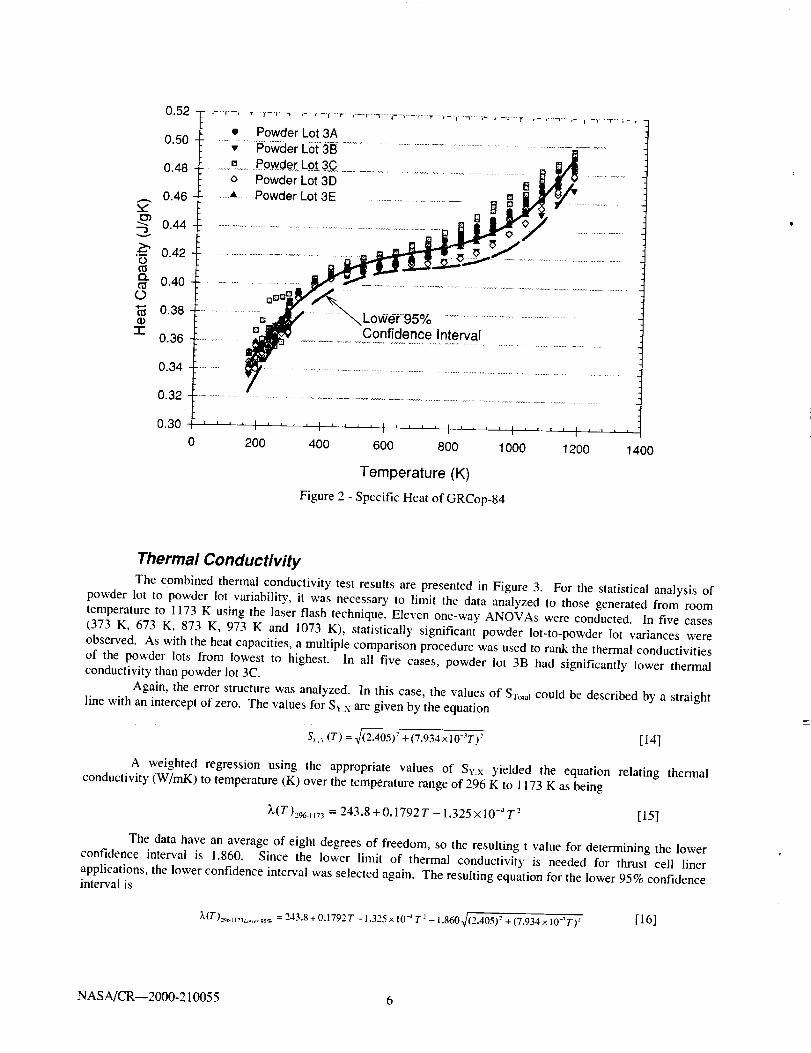
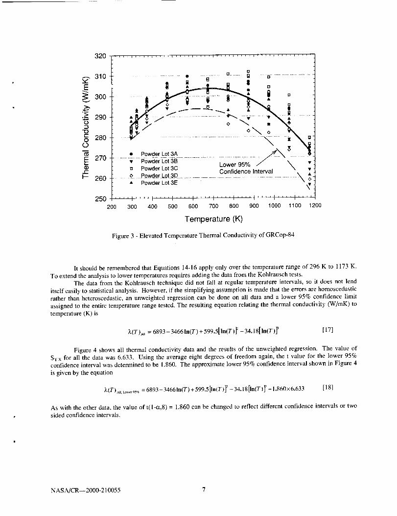
Thermal Conductivity
The combined thermal conductivity test results are presented in Figure 3. For the statistical analysis ofpowder lot to powder lot variability, it was necessary to limit the data analyzed to those generated from roomtemperature to 1173 K using the laser flash technique. Eleven one-way ANOVAs were conducted. In five cases(373 K, 673 K, 873 K, 973 K and 1073 K), statistically significant powder lot-to-powder lot variances were
observed. As with the heat capacities, a multiple comparison procedure was used to rank the thermal conductivities
of the powder lots from lowest to highest. In all five cases, powder lot 3B had significantly lower thermalconductivity than powder lot 3C.
Again, the error structure was analyzed. In this case, the values of STota I could be described by a straightline with an intercept of zero. The values for Svx are given by the equation
S,._ (T) = _](2.405) -_+(7.934x10-_T) -" [14]
A weighted regression using the appropriate values of Svx yielded the equation relating thermalconductivity (W/mK) to temperature (K) over the temperature range of 296 K to 1173 K as being
X(T)2961j73 = 243.8 +0.1792 T -l.325x10-"T -_ [15]
The data have an average of eight degrees of freedom, so the resulting t value for determining the lowerconfidence interval is 1.860. Since the lower limit of thermal conductivity is needed for thrust cell liner
applications, the lower confidence interval was selected again. The resulting equation for the lower 95% confidenceinterval is
_'(T) 29_]_73L,,,,_,9_, = 243.8 + 0.1792 T - ] .325 x 10 "_T "_- 1.860 _(2.405F" + (7.934 x 10-aT) z [16]
NAS A/CR--2000-210055 6
[]
......... r_...... g . 0- ............................---310 ..........................• g
300 1290 .......................
280 ....
('_ • Powder Lot 3A .,_,_ v j
_ 270 ................... ................................. ........ ........_ ....... ,, v-JPowcJer'L-ot3B..... .. Lower uo zo / \ i
m Howoer LOIL_U .... In" rval \ • 4
260 A Powder Lot 3E ,_
-t250 .... .... ',.... , .... .... ',..... .... : .... I .... ,'
200 300 400 500 600 700 800 900 1000 1100 1200
Temperature (K)
Figure 3 - Elevated Temperature Thermal Conductivity of GRCop-84
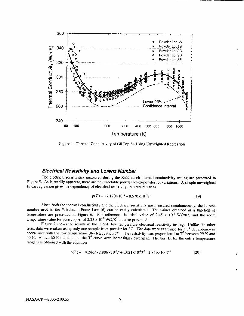
It should be remembered that Equations 14-16 apply only over the temperature range of 296 K to 1173 K.
To extend the analysis to lower temperatures requires adding the data from the Kohlrausch tests.The data from the Kohlrausch technique did not fall at regular temperature intervals, so it does not lend
itself easily to statistical analysis. However, if the simplifying assumption is made that the errors are homoscedasticrather than heteroscedastic, an unweighted regression can be done on all data and a lower 95% confidence limit
assigned to the entire temperature range tested. The resulting equation relating the thermal conductivity (W/mK) to
temperature (K) is
X(T),_, = 6893- 3466 In(r) + 599.5[In(T)]_ - 34.18[In(T)]_ [17]
Figure 4 shows all thermal conductivity data and the results of the unweighted regression. The value of
Sv.x for all the data was 6.633. Using the average eight degrees of freedom again, the t value for the lower 95%confidence interval was determined to be 1.860. The approximate lower 95% confidence interval shown in Figure 4
is given by the equation
_,(T)AIIILO,.,,,r95% = 6893_ 3466In(T) +599.5[I,(T)] e _34.18[In(T)]_ _1.860x6.633 [18]
As with the other data, the value of t(l-c_,8) = 1.860 can be changed to reflect different confidence intervals or two
sided confidence intervals.
NASA/CR--2000-210055 7
360 ,
,_" 340
v
._, 320
o"_ 300
"ot-o
(..)
-_ 280
Ed::I-- 260
240
• Powder Lot 3Ao• • Powder Lot 3B
• [_ Powder Lot 3Co Powder Lot 3D
A Powder Lot 3E
• j----J
Jj Lower 95%
..............................._/ ............................ Confidence Interval ..............
80i f i i i i I
100 200 300 400 500 600 800 1000
Temperature (K)
Figure 4 - Thermal Conductivity of GRCop-84 Using Unweighted Regression
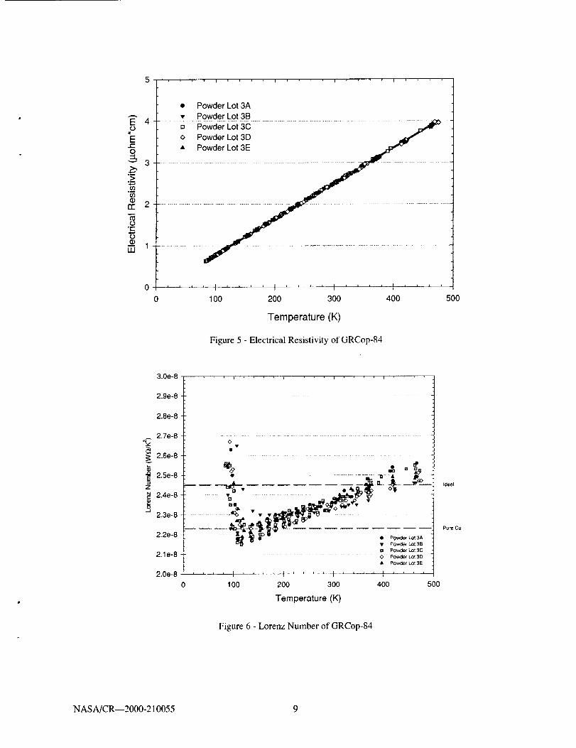
Electrical Resistivity and Lorenz Number
The electrical resistivities measured during the Kohlrausch thermal conductivity testing are presented in
Figure 5. As is readily apparent, there are no detectable powder lot-to-powder lot variations. A simple unweightedlinear regression gives the dependency of electrical resistivity on temperature as
p(T) =-7.170x10 -2 +8.570x10⁻³T [19]
Since both the thermal conductivity and the electrical resistivity are measured simultaneously, the Lorenznumber used in the Wiedmann-Franz Law (6) can be easily calculated. The values obtained as a function of
temperature are presented in Figure 6. For reference, the ideal value of 2.45 x 10 .8 Wf2/K 2, and the room
temperature value for pure copper of 2.23 x 10 -8 W_/K 2 are also presented.
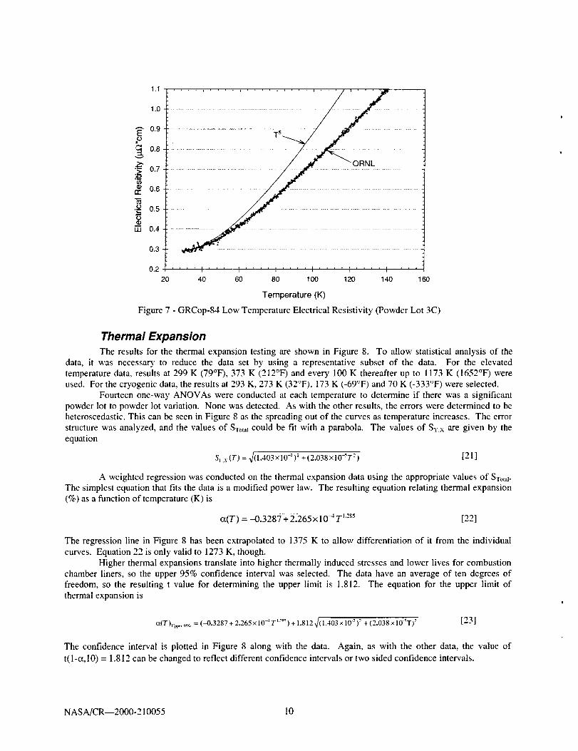
Figure 7 shows the results of the ORNL low temperature electrical resistivity testing. Unlike the other
tests, data were taken using only one sample from powder lot 3C. The data were examined for a T 5 dependency inaccordance with the low temperature Bloch Equation (7). The resistivity was proportional to T -_between 29 K and40 K. Above 60 K the data and the T 5 curve were increasingly divergent. The best fit for the entire temperaturerange was obtained with the equation
p(T)= 0.2865-2.886×lO-3T + l.O21xlO4T2-2.859×lO-TT 3 [20]
NAS A/CR--2000-210055 8
E(D
"Et-O
v
..1.-,
O3
n-
,.i.-,
LU
0
0
• Powder Lot 3A• Powder Lot 3B
[] Powder Lot 3Co Powder Lot3D• Powder Lot 3E
100 200 300
Temperature (K)
Figure 5 - Electrical Resistivity of GRCop-84
400 5OO
3.0e-8
2.9e-8
2.8e-8
2.7e-8
_ 2.6e-8
_ 2.5e-8
Z
_: 2.4e-8O._1
2.3e-8
2.2e-8
2.1e-8
2.0e-8
i i
O
0 v
_._ . ,.=..-.o_:'_.'_,•_ .....
i_ 1_ _>w ,, P;wd;iLoi3A13_. • Powder Lot 3B
Powder Lot 3C
O Powder Lot 3D
• Powder Lot 3E
', I 4 .... I ....100 200 300 400 500
Temperature (K)
Ideal
Pure Cu
Figure 6 - Lorenz Number of GRCop-84
NAS A/CR--2000-210055 9
EO
¢d)
r'e-
_.oIII
1.1 i _ _ .... i . , , i ........
1.0 ...............................................................................................................................
0.9 ..................................................... T5 .............................
0.8
0.7
0.6
0.5
0.3
o.2 .... ', .... I .... : .... I .... : .... : ....20 40 60 80 1O0 120 140 160
Temperature (K)
Figure 7 - GRCop-84 Low Temperature Electrical Resistivity (Powder Lot 3C)
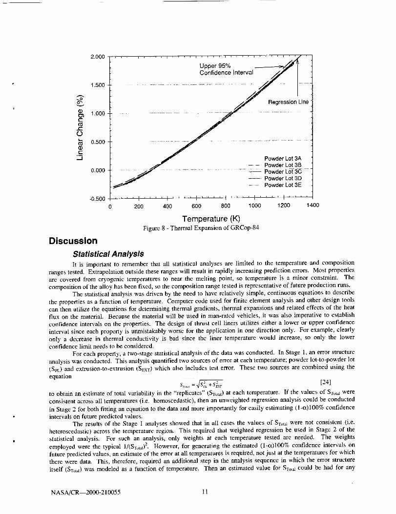
Thermal ExpansionThe results for the thermal expansion testing are shown in Figure 8. To allow statistical analysis of the
data, it was necessary to reduce the data set by using a representative subset of the data. For the elevated
temperature data, results at 299 K (79°F), 373 K (212°F) and every 100 K thereafter up to 1173 K (1652°F) were
used. For the cryogenic data, the results at 293 K, 273 K (32°F), 173 K (-69°F) and 70 K (-333°F) were selected.
Fourteen one-way ANOVAs were conducted at each temperature to determine if there was a significant
powder lot to powder lot variation. None was detected. As with the other results, the errors were determined to be
heteroscedastic. This can be seen in Figure 8 as the spreading out of the curves as temperature increases. The error
structure was analyzed, and the values of STo,,_ could be fit with a parabola. The values of Syx are given by the
equation
S_ .x (T) = x/(1.403 × 10-" )" + (2.038 x 10-_T ') [21 ]
A weighted regression was conducted on the thermal expansion data using the appropriate values of STo,,I.
The simplest equation that fits the data is a modified power law. The resulting equation relating thermal expansion
(%) as a function of temperature (K) is
offT) = -0.3287 + 2.265x 10 -4 T TM [22]
The regression line in Figure 8 has been extrapolated to 1375 K to allow differentiation of it from the individual
curves. Equation 22 is only valid to 1273 K, though.
Higher thermal expansions translate into higher thermally induced stresses and lower lives for combustion
chamber liners, so the upper 95% confidence interval was selected. The data have an average of ten degrees of
freedom, so the resulting t value for determining the upper limit is 1.812. The equation for the upper limit of
thermal expansion is
_(T)um, 9_¢. = (_0.3287 + 2.265 × 10 -_ T t..'_ ) + 1.812 _/(1,403 x I0" )-" + (2.038 x 10-_T) 2[23]
The confidence interval is plotted in Figure 8 along with the data. Again, as with the other data, the value of
t(1-e_,10) = 1.812 can be changed to reflect different confidence intervals or two sided confidence intervals.
NASA/CR--2000-210055 10
2.000
Upper 95%Confidence Interval
i .500 ..............................................................................................
v
e-
t-O
(1)r-_J
1.000
0.500
0.000
Regression Line
Powder Lot 3APowder Lot 3B
........................................................................ Pbwder Lot 3C ........ Powder Lot 3D...... Powder Lot 3E
-0.5000 2oo 4oo 6oo 8oo i 000 12oo 14oo
Temperature (K)Figure 8 - Thermal Expansion of GRCop-84
Discussion
Statistical AnalysisIt is important to remember that all statistical analyses are limited to the temperature and composition
ranges tested. Extrapolation outside these ranges will result in rapidly increasing prediction errors. Most propertiesare covered from cryogenic temperatures to near the melting point, so temperature is a minor constraint. The
composition of the alloy has been fixed, so the composition range tested is representative of future production runs.The statistical analysis was driven by the need to have relatively simple, continuous equations to describe
the properties as a function of temperature. Computer code used for finite element analysis and other design toolscan then utilize the equations for determining thermal gradients, thermal expansions and related effects of the heatflux on the material. Because the material will be used in man-rated vehicles, it was also imperative to establish
confidence intervals on the properties. The design of thrust cell liners utilizes either a lower or upper confidence
interval since each property is unmistakably worse for the application in one direction only. For example, clearly
only a decrease in thermal conductivity is bad since the liner temperature would increase, so only the lowerconfidence limit needs to be considered.
For each property, a two-stage statistical analysis of the data was conducted. In Stage 1, an error structure
analysis was conducted. This analysis quantified two sources of error at each temperature; powder lot-to-powder lot(SEE) and extrusion-to-extrusion (SExT) which also includes test error. These two sources are combined using the
equationST,,,,,,= _ [24]
to obtain an estimate of total variability in the "replicates" (Sxot,l) at each temperature. If the values of STot_ were
consistent across all temperatures (i.e. homoscedastic), then an unweighted regression analysis could be conducted
in Stage 2 for both fitting an equation to the data and more importantly for easily estimating (1-_)100% confidenceintervals on future predicted values.
The results of the Stage 1 analyses showed that in all cases the values of STot,i were not consistent (i.e.heteroscedastic) across the temperature region. This required that weighted regression be used in Stage 2 of the
statistical analysis. For such an analysis, only weights at each temperature tested are needed. The weights
employed were the typical 1/(STo,,02. However, for generating the estimated (1-_)100% confidence intervals on
future predicted values, an estimate of the error at all temperatures is required, not just at the temperatures for whichthere were data. This, therefore, required an additional step in the analysis sequence in which the error structure
itself (STot,0 was modeled as a function of temperature. Then an estimated value for STot,l could be had for any
NASA/CR--2000-210055 11
temperature.ThesepredictedSTot_lvalueswereusedincalculatingtheweightsfortheweightedregression.Theywerealsousedincalculatingtheestimated(I-cz)100%confidenceintervalsonfuturepredictedvaluesasshownintheResultssection.
As mentionedbefore,thewidthsof the estimated (1-cz)100% confidence intervals on future predicted
values are simply t(1-o¢,v)Sv.x. Sv.x is made up of two components; pure error and lack-of-fit (LOF). The pureerror component, STot,I, was estimated in Stage 1 and was found to be heteroscedastic. Hence, Sv.x could not be
estimated in the usual way (i.e. Equation 5), but had to be manufactured from STo_ and an estimate of the LOFcomponent as shown in Equation 7. The LOF component measures how far off the model predictions are from the
mean of properly Y replicates. A "good" model, i.e., one without significant LOF, should have close agreement
between the mean value of the response and the predicted value of the response. The LOF component wasestimated using Equation 6. Lastly and specific to this work, a heteroscedastic standard error of the regression as a
function of temperature, Svx(T), was manufactured from the estimated heteroscedastic pure error componentSTotal(T ) and the estimated LOF component using Equation 7. This value of Svx(T) was then used to calculate the
width of the estimated (1-oc)100% confidence intervals on future predicted values as just t(1-c_,v)Sy x(T).Notice that the t value is also important in setting the confidence interval. In this case, one-sided 95%
confidence intervals were generated for all the properties. Changing the confidence level can be easilyaccomplished by substituting the t value for the same number of degrees of freedom (v) but a different confidence
level (l-c0. However, it must be remembered that a simplifying assumption was made to use an integral averagenumber of degrees of freedom rather than the degrees of freedom at each temperature. To determine the effects of
the degrees of freedom on the t value, the worst case, specific heat, was examined. The lowest number of degrees offreedom from the Satterthwaite's formula was 5.3 at 1073 K. An average of eight degrees of freedom was used forthe determination of the confidence interval. From a table of t values, the t value at a 95% confidence level would
increase from 1.860 to 2.015 if five degrees of freedom are used. This represents a change of 8.3%. Therefore, the
error term in Equation 9 would increase from 0.0180 J/gK to 0.0195 J/gK at 1073 K. On the scale of Figure 2, thisrepresents lowering the confidence interval one minor division on the Y axis. It also represents less than 0.5%
change in the value for the confidence interval. The results are similar for other temperatures where the degrees offreedom are less than eight. Based on this, the decision to use an average degrees of freedom was deemed to bejustified.
Finally, it must be pointed out that because of the methods used and the simplifying assumptions, strictly
speaking, the confidence intervals are estimates. However, because of the large number of data points generatedduring testing, simple comparison of the confidence intervals to the data can reveal if the estimates are valid. For a
95% confidence interval, if one hundred data points are plotted five should fall outside the confidence interval, e.g.,five data points would be below a lower confidence interval. Examining Figures 1, 2 and 3, the total number of data
points were 165,390 and 165 respectively. It would be expected that 8, 20 and 8 data points would fall outside theconfidence interval if it is truly a 95% confidence interval. In fact, only 6, 6 and 3 data points fall outside the
confidence intervals. In the case of thermal expansion, a subset of the data was used for the regression andconfidence interval. Even so, the upper 95% confidence interval encompasses all but a few data points from thecomplete data set. Based on these observations, the confidence intervals are in fact conservative for a 95%
confidence interval and can be used for design purposes.
Specific Heat
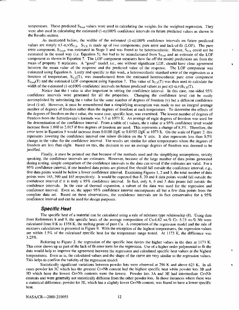
The specific heat of a material can be calculated using a rule of mixtures type relationship (8). Using datafrom References 8 and 9, the specific heats of the average composition of Cu-6.62 wt.% Cr- 5.73 wt.% Nb werecalculated from 0 K to 1358 K, the melting point of pure Cu. A comparison of the regression model and the rule of
mixtures calculations is presented in Figure 9. With the exception of the highest temperatures, the regression valuesare within 1.5% of the calculated specific heat for the temperature range tested. At 1173 K, the difference was3.25%.
Referring to Figure 2, the regression of the specific heat favors the higher values in the data at 1173 K.
This error shows up as part of the lack of fit error term for the regression. Use of a higher order polynomial to fit thedata would help to improve the agreement between the regression and calculated specific heat values at the highest
temperatures. Even as is, the calculated values and the shape of the curve are very similar to the regression values.This helps to confirm the validity of the regression model.
Statistically significant variations between powder lots were observed at 296 K and above 623 K. In allcases powder lot 3C which has the greatest Cr+Nb content had the highest specific heat while powder lots 3B and3D which have the lowest Cr+Nb contents were the lowest. Powder lots 3A and 3E had intermediate Cr+Nb
contents and were generally not statistically different from the other powder lots. In those instances where there was
a statistical difference, powder lot 3E, which has a slightly lower Cr+Nb content, was found to have a lower specificheat.
NASA/CR--2000-210055 12
Fromthisanalysis,it canbeseenthat,eventhoughtherangeof Cr+Nbcontentsissmall(0.22wt.%),thesensitivityof thetestmethodmadeit possibletodetectdifferencesatcertaintemperatures.In practicalterms,thevariationsinspecificheatfromthevariationsinCr+Nbcontentsissmallandisaccountedforbyusingthevaluesofthe lowerconfidenceintervalinadesign.
0.60
0.5O
.-j
"1-
o. 0.4009
0.30/11 i_, i i R'O'M" Calculated ce
'' ' I .... ', .... I .... : .... ', '
200 400 600 800 1000 1200
Temperature (K)Figure 9 - Comparison of Regression and Calculated Specific Heat Values
1400
Thermal Conductivity
In five cases, it was determined that there was a statistically significant difference in the thermal
conductivity between powder lots. Referring back to the specific heat, most of the temperatures where the thermal
conductivity is different correspond to the temperature range where differences were observed in the specific heats.From Equation 1, it is known that the thermal conductivity is proportional to the specific heat. It is therefore not
surprising that the thermal conductivity shows lot-to-lot variations when the specific heat does. The same generalrankings are observed as with the specific heat as well. Again, the sensitivity of the test method is sufficient todetect the small variations caused by the slight differences in chemistry. These differences are accounted for by
using the lower confidence interval in a design.The thermal conductivity of high purity Cu is 397 W/mK at room temperature (10). As shown in Figure 3,
the thermal conductivity of GRCop-84 at room temperature is lower than pure Cu. However, it is still much higherthan many materials with similar elevated temperature mechanical properties such as stainless steels (11).
The lower thermal conductivity relative to pure Cu is a concern since lowering the thermal conductivityincreases the operating temperature. However, prior work (1-3) has shown GRCop-84 has significantly greater
strength and maximum operating temperature capability. Using a yield strength of 100 MPa as the criteria formaximum operating temperature, GRCop-84 can be used up to 973 K while NARloy-Z is limited to 773 K. The
lower thermal conductivity of GRCop-84 should translate into a much smaller temperature increase than 200 K.Therefore, the lower thermal conductivity should not preclude the use of GRCop-84 in thrust cell liners and many
other applications.In addition, the significantly higher strength of GRCop-84 can be used to redesign components. Since the
strength of GRCop-84 is approximately twice that of NARloy-Z at 773 K, the cooling channel wails can be thinnedwhile still maintaining a considerable safety margin. Therefore, while the lower thermal conductivity will increasethe thermal gradient, thinning the walls may actually result in a lower hot wall temperature.
Currently the Rocketdyne Division of Boeing is conducting trade studies using the recently generated data
to determine the effects of lowering the thermal conductivity. The chemical analysis of the extrusions shown inTable 1 also suggests another method to increase thermal conductivity through lowered impurity content.
NASA/CR--2000-210055 13
Effect of Fe
The effect of Fe on the thermal conductivity cannot be directly determined at this point because the Fe
contents of the five powder lots tested were very similar. However, using the effect of Fe on electrical resistivity asa guide, the relative effect of Fe on thermal conductivity may be assessed.
Pawlek and Reichel (12) reported a room temperature electrical resistivity of 1.68 p,Q*cm for pure Cu. The
addition of 0.0150 wt.% Fe increases the electrical resistivity to 1.86 p,Q*cm. Applying the Weidmann-Franz Law,
this corresponds to a decrease in thermal conductivity of 11% or about 44 W/mK. In the GRCop-84 samples tested,
the decreases in room temperature thermal conductivity relative to pure Cu average 115 W/InK. Therefore, thedecrease from the Fe impurities alone could account for 38% of the total decrease in thermal conductivity.
This analysis does not take into account the possibility the Fe is present exclusively in the CrzNb particlesnor does it examine the possibility the Fe forms Fe-Cr precipitates. Both situations would not affect the thermal
conductivity as severely as Fe being present in the Cu matrix. However, it does indicate the potential for a
significant increase in thermal conductivity for the alloy. The economical viability of producing lower Fe contentalloys may preclude its use for commercial applications, though.
Effect of Thermal Conductivity on Lorenz Number
The Lorenz number is generally referred to as a constant. However, Figure 6 clearly shows the value is
dependent on temperature. Above approximately 120 K the Lorenz number slowly increases linearly with
temperature. Below 120 K the Lorenz number rapidly increases. The deviation from a constant value can be tracedto the changes in the thermal conductivity shown in Figure 4.
Between 120 K and 473 K, the thermal conductivity is slowly increasing in a near linear manner. The
relative change is only slightly greater than that of the electrical resistivity. Consequently, the Lorenz number is
increasing very slowly and could be considered constant. Below 120 K the thermal conductivity is rapidlyincreasing while the electrical resistivity continues to decrease linearly. Therefore, the Lorenz number rapidlyincreases.
The cause of the rapid increase in the thermal conductivity is related to the effects of imperfections such asdislocations and solute atoms on thermal conductivity. White (13) showed that pure Ag had two different
dependencies of thermal conductivity on temperature based on the imperfections. A heavily deformed Ag sampleshowed no thermal conductivity maxima, but the same sample when annealed showed a maximum near 20 K.
Above 20 K the thermal conductivity rapidly decreased and asymptotically approached a constant value above 50 K.The same basic behavior is observed in Figure 4 for GRCop-84. The differing behavior for Ag was attributed to the
changing concentration of imperfections, in this case dislocations.Matthiessen's Rule (14), which deals with the electrical resistivity of a metal, can be used to examine
scattering of the electrons by static imperfections and phonons. In its general form, Matthiessen's Rule can be
expressed as
p(T) = Po +p,(T) [25]
where po is equal to the scattering from imperfections and pi(T) is the scattering from phonons. The scattering from
imperfections is dependent on the concentration of imperfections but is independent of temperature. Figure 5 andEquation 19 indicate that GRCop-84 follows Matthiessen's Rule.
An analogous situation exists with the thermal resistivity (W). The thermal resistivity is given by the
equationI
W (T) = -- = l_o (T) +W, (T) [2613,(T)
where Wo(T) is the thermal resistivity from the imperfections and Wi(T) is the thermal resistivity from the electron-
phonon interactions.Since the imperfections generally scatter the electrons elastically, the Wiedemann-Franz Law and the ideal
value of the Lorenz number can be used to relate WOO') to Po. From this, it can be shown that the temperature
dependency of Wo(T) is proportional to 1/1".Since both Wo and W_ are dependent on temperature, the relative rates of change determine if there is a
thermal conductivity maximum. If the value of Wo is near Wi at low temperatures, then the relative changes in thetwo values (lff versus T) results in a maximum in the thermal conductivity followed by a decrease to a limiting
value. On the other hand, if a metal or alloy has a large imperfection concentration, then Wi and Wo become
comparable only at high temperatures where Wo is already essentially constant. In this case, as shown by White, thethermal conductivity increases and asymptotically approaches the limiting value.
In the case of GRCop-84, the thermal conductivity will go through a maximum at some temperature below
50 K, probably near 30 K, the value for pure Cu (15). This indicates that the contribution from the imperfections to
the thermal resistivity is low and comparable to the electron-phonon interactions only at very low temperatures. The
NAS A/CR--2000-210055 14
alloywasdesignedsuchthatthematrixwouldbenearlypureCu.FromtheanalysisofthethermalconductivityandLorenznumber,it appearsthatthisgoalwasachieved.It alsoindicatesthattheconcentrationofdislocationsis lowalthoughthematerialwashighlydeformedduringtheextrusionprocess.Fromthisit canbeinferredthatGRCop-84isatleastpartiallyandprobablyfullyrecrystallized.
Low Temperature Electrical Resistivity
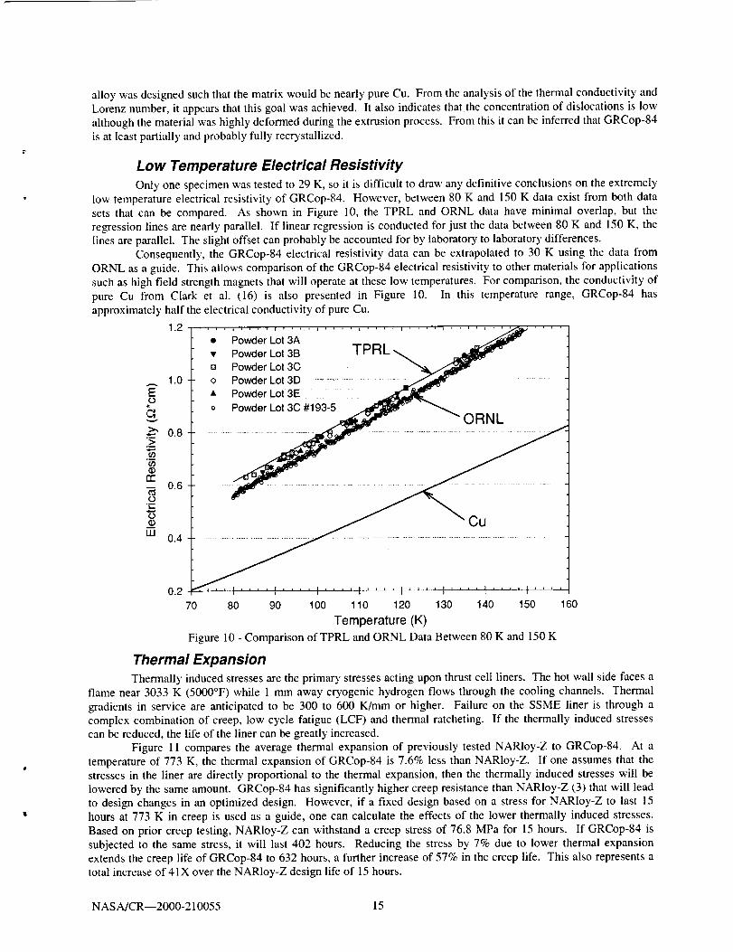
Only one specimen was tested to 29 K, so it is difficult to draw any definitive conclusions on the extremely
low temperature electrical resistivity of GRCop-84. However, between 80 K and 150 K data exist from both datasets that can be compared. As shown in Figure 10, the TPRL and ORNL data have minimal overlap, but the
regression lines are nearly parallel. If linear regression is conducted for just the data between 80 K and 150 K, thelines are parallel. The slight offset can probably be accounted for by laboratory to laboratory differences.
Consequently, the GRCop-84 electrical resistivity data can be extrapolated to 30 K using the data from
ORNL as a guide. This allows comparison of the GRCop-84 electrical resistivity to other materials for applicationssuch as high field strength magnets that will operate at these low temperatures. For comparison, the conductivity of
pure Cu from Clark et al. (16) is also presented in Figure 10. In this temperature range, GRCop-84 has
approximately half the electrical conductivity of pure Cu.
E¢.9
v
,.t..a
>.w
t/)t9rr
t_ok.
.9.0ILl
• Powder Lot 3A• Powder Lot 3B[] Powder Lot 3C<> Powder Lot 3D ...........................
• Powder Lot3E
o Powder Lot 3C #193-5ORNL
Cu
0.2
70 80 90 100 110 120 130 140 150
Temperature (K)
Figure 10 - Comparison of TPRL and ORNL Data Between 80 K and 150 K
Thermal Expansion
160
Thermally induced stresses are the primary stresses acting upon thrust cell liners. The hot wall side faces aflame near 3033 K (5000°F) while 1 mm away cryogenic hydrogen flows through the cooling channels. Thermal
gradients in service are anticipated to be 300 to 600 K/mm or higher. Failure on the SSME liner is through a
complex combination of creep, low cycle fatigue (LCF) and thermal ratcheting. If the thermally induced stressescan be reduced, the life of the liner can be greatly increased.
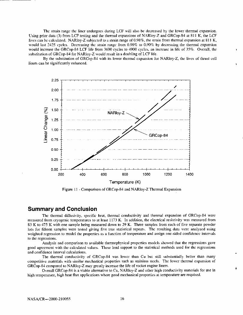
Figure 11 compares the average thermal expansion of previously tested NARIoy-Z to GRCop-84. At a
temperature of 773 K, the thermal expansion of GRCop-84 is 7.6% less than NARloy-Z. If one assumes that thestresses in the liner are directly proportional to the thermal expansion, then the thermally induced stresses will be
lowered by the same amount. GRCop-84 has significantly higher creep resistance than NARIoy-Z (3) that will leadto design changes in an optimized design. However, if a fixed design based on a stress for NARloy-Z to last 15
hours at 773 K in creep is used as a guide, one can calculate the effects of the lower thermally induced stresses.Based on prior creep testing, NARIoy-Z can withstand a creep stress of 76.8 MPa for 15 hours. If GRCop-84 is
subjected to the same stress, it will last 402 hours. Reducing the stress by 7% due to lower thermal expansionextends the creep life of GRCop-84 to 632 hours, a further increase of 57% in the creep life. This also represents a
total increase of 41X over the NARloy-Z design life of 15 hours.
NASA/CR--2000-210055 15
ThestrainrangethelinerundergoesduringLCFwill alsobedecreasedbythelowerthermalexpansion.Usingpriordata(3)fromLCFtesting and the thermal expansions of NARloy-Z and GRCop-84 at 811 K, the LCFlives can be calculated. NARloy-Z subjected to a strain range of 0.98%, the strain from thermal expansion at 811 K,
would last 2425 cycles. Decreasing the strain range from 0.98% to 0.90% by decreasing the thermal expansionwould increase the GRCop-84 LCF life from 3600 cycles to 4900 cycles, an increase in life of 35%. Overall, the
substitution of GRCop-84 for NARloy-Z would result in a doubling of LCF life.By the substitution of GRCop-84 with its lower thermal expansion for NARIoy-Z, the lives of thrust ceil
liners can be significantly enhanced.
v
(D
t-t_
e"(.)
(D
...J
2.25
2.00
1.75
1.50
1.25
1.00
0.75
0.50
0.25
0.00
/
NARIoy-Z
GRCop-84
200 400 600 800 1000 1200
Temperature (K)
Figure 11 - Comparison of GRCop-84 and NARloy-Z Thermal Expansion
1400
Summary and ConclusionThe thermal diffusivity, specific heat, thermal conductivity and thermal expansion of GRCop-84 were
measured from cryogenic temperatures to at least 1173 K. In addition, the electrical resistivity was measured from
83 K to 475 K with one sample being measured down to 29 K. Three samples from each of five separate powderlots for fifteen samples were tested giving five true statistical repeats. The resulting data were analyzed using
weighted regression to model the properties as a function of temperature and assign one-sided confidence intervalsto the regressions.
Analysis and comparison to available thermophysical properties models showed that the regressions gavegood agreement with the calculated values. These lend support to the statistical methods used for the regressionsand confidence interval calculations.
The thermal conductivity of GRCop-84 was lower than Cu but still substantially better than manycompetitive materials with similar mechanical properties such as stainless steels. The lower thermal expansion of
GRCop-84 compared to NARIoy-Z may greatly increase the life of rocket engine liners.
Overall GRCop-84 is a viable alternative to Cu, NARloy-Z and other high conductivity materials for use inhigh temperature, high heat flux applications where good mechanical properties at temperature are required.
NASA]CR--2000-210055 16
References1. D.L. Ellis and R.L. Dreshfield, "Preliminary Evaluation of a Powder Metal Copper-8 Cr-4 Nb
Alloy," Proc. of the Advanced Earth-to-Orbit Conference, NASA CP-3174, NASA MSFC,
Huntsville, AL, (May 1992)2. D.L. Ellis, R.L. Dreshfield, M.J. Verrilli, and D.G. Ulmer, "Mechanical Properties of a Cu-8
Cr-4 Nb Alloy," Earth-to-Orbit Conference, NASA CP-3282, NASA MSFC, Huntsville, AL
(May 1 994)3. D.L. Ellis and G.M. Michal, Mechanical and Thermal Properties of Two Czt-Cr-Nb Alloys and NARIoy-Z,
NASA CR 198529, NASA Lewis Research Center, Cleveland, OH, (Oct. 1996)
4. M.A. Buckman, L.D. Bentsen, J. Makosey, G.R. Angell and D.P.H Hasselman, Trans. Brit. Cer. Soc., Voi. 82,
No. 1, (1983), pp.18-235. P.G. Klemens, Thermal Condtlctivity, Vol. 1, ed. R.P. Tye, Academic Press, London and New York, 1969, p.
37.
6. Transport Phenomena in Metalhtrgy, G.H. Geiger and D.R. Poirier, Addison-Wesley Publ. Co., Reading, MA,
(1973), p. 1917. F. Bloch, Z. Physik, Vol. 59, (1930), p. 208
8. R.R. Hultgreen, Selected Values of Thermodynamic Properties of the Elements, ASM International, MetalsPark, OH (1973)
9. NIST-JANAF Thermochemical Tables, Fow'th Ed., Part H, Cr-Zr, M.W. Chase, Jr. Ed., American Institute
of Physics for the National Institute of Standards and Technology, Washington, DC (1998)10. Smithells Metals Reference Book, 6 thEd., E.A. Brandes, Ed., Butterworths, London, (1983), p. 14-1
11. Smithells Metals Reference Book, 6 'j' Ed., E.A. Brandes, Ed., Butterworths, London, (1983), pp. 14-23 to 14-3912. F. Pawlek and K. Reichel, "The Effect of Impurities On The Electrical Conductivity of Copper," Zeit.
Metallkunde, Vol. 47, (1956), p. 347
13. G.K. White, Proc. Phys. Soc. London, Vol. A66, (1953), p. 84414. A. Matthiessen and C. Vogt, Ann. Phys. Leibz, Vol. 122, (1964), p. 1915. F.R. Schwartzberg, S.H. Osgood, R.O. Keys and T.F. Kiefer, C1Togenic Materials Data Handbook, The Martin
Co., (Aug. 1964)16. A.F. Clark, G.E. Childs and C.H. Wallace, "Low Temperature Electrical Resistivity of Some Engineering
Alloys," Cryogenic Materials Conference, Univ. of California, (June 1969)
NASA/CR--2000-210055 17
REPORT DOCUMENTATION PAGE FormApprovedOMB No. 0704-0188
Public reporting burden for this collection of information is estimated to average 1 hour per response, including the time for reviewing instructions, searching existing data sources,
gathering and maintaining the data needed, and completing and reviewing the collection of information. Send comments regarding this burden estimate or any other aspect of this
collection of information, including suggest!ons for reducing this burden, to Washington Headquarters Services, Directorste for Information Operations and Reports, 1215 Jefferson
Davis Highway, Suite 1204, Arlington, VA 22202-4302, and to the Office of Management and Budget, Paperwork Reduction Project (0704-0188), Washington, DC 20503.
1. AGENCY USE ONLY (Leave blank) 2. REPORT DATE 3. REPORTTYPE AND DATES COVERED
June 2000 Final Contractor Report4. TITLE AND SUBTITLE
Thermophysical Properties of GRCop-84
6. AUTHOR(S)
David L. Ellis and Dennis J. Keller
PERFORMING ORGANIZATION NAME(S) AND ADDRESS(ES)
Case Western Reserve University
White Building
10900 Euclid Avenue
Cleveland, Ohio 44106--7204
9. SPONSORING/MONITORING AGENCY NAME(S) AND ADDRESS(ES)
National Aeronautics and Space Administration
John H. Glenn Research Center at Lewis Field
Cleveland, Ohio 44135-3191
11. SUPPLEMENTARY NOTES
5. FUNDING NUMBERS
WU-242-23-54-00
NAS3--463
8. PERFORMING ORGANIZATIONREPORT NUMBER
E-12257
10. SPONSORING/MONITORINGAGENCY REPORT NUMBER
NASA CR--2000-210055
David L. Ellis, Case Western Reserve University, White Building, 10900 Euclid Avenue, Cleveland, Ohio 44106-7204; and
Dennis J. Keller, RealWorld Quality Systems, Inc., 20388 Bonnie Bank Blvd., Cleveland, Ohio 44116. Project Manager,
Michael Nathal, Materials Division, NASA Glenn Research Center, organization code 5120, (216) 433-9516.
12a. DISTRIBUTION/AVAILABILITY STATEMENT
Unclassified - Unlimited
Subject Category: 26 Distribution: Nonstandard
This publication is available from the NASA Center for AeroSpace Information, (301) 621-0390.
12b. DISTRIBUTION CODE
13. ABSTRACT (Maximum 200 words)
The thermophysical properties and electrical resistivity of GRCop-84 (Cu - 8 at.% Cr-4 at.% Nb) were measured from
cryogenic temperatures to near its melting point. The data were analyzed using weighted regression to determine the
properties as a function of temperature and assign appropriate confidence intervals. The results showed that the thermal
expansion of GRCop-84 was significantly lower than NARloy-Z (Cu-3 wt.% Ag-0.5 wt.% Zr), the currently used thrust
cell liner material. The lower thermal expansion is expected to translate into lower thermally induced stresses and in-
creases in thrust cell liner lives between 2X and 4IX over NARloy-Z. The somewhat lower thermal conductivity of
GRCop-84 can be offset by redesigning the liners to utilize its much greater mechanical properties. Optimized designs are
not expected to suffer from the lower thermal conductivity. Electrical resistivity data, while not central to the primary
application, show that GRCop-84 has potential for applications where a combination of good electrical conductivity and
strength is required.
14. SUBJECT TERMS
Thermal conductivity; Electrical resistivity; Specific heat; Thermal diffusivity; Cu alloys
17. SECURITY CLASSIFICATIONOF REPORT
Unclassified
NSN 7540-01-280-5500
18. SECURITY CLASSIFICATIONOF THIS PAGE
Unclassified
19. SECURITY CLASSIFICATIONOF ABSTRACT
Unclassified
15. NUMBER OF PAGES23
16. PRICE CODE
A03
20. LIMITATION OF ABSTRACT
Standard Foml 298 (Rev. 2-89)Prescribed by ANSI Std. z3g-18298-102