Embed Size (px)
Citation preview
Three-Dimensional Nonlinear Dynamics of Cantilevered
Cylinders in Axial Flow
by
Ahmad Jamal
Department of Mechanical Engineering
McGill University
Montréal, Quebec, Canada
April 2014
A thesis submitted to McGill University
in partial fulfillment of the requirements of the degree of
Doctor of Philosophy
© Ahmad Jamal 2014
i
Abstract
This thesis deals with the theoretical study of the linear and nonlinear dynamics of a slender
flexible cantilevered cylindrical structure subjected to external axial water and air flows, of
interest because of several important practical applications such as nuclear reactor fuel-element
bundles, double pipe heat exchangers, and angioplasty. Lack of knowledge to account for the
three-dimensional behaviour, important in the above-mentioned practical applications, was the
motivation behind the present work. The theoretical results were obtained in the form of the
amplitudes and frequencies of the instabilities, as well as the critical flow velocities at which
these instabilities occurred.
Experiments were conducted to validate and complement the theoretical results for water
flow. The results obtained from the experiments were presented in the form of dimensionless
mean displacements, their corresponding root mean square values, and frequencies as a function
of dimensionless flow velocity. Finally, the path traced by the oscillating cylinder was mapped.
In fluid-structure interaction problems, the fluid forces such as the inviscid
hydrodynamic forces, the frictional or viscous forces, and the hydrostatic or pressure forces
acting on the flexible structure play a vital role in defining the dynamics of the system.
Therefore, a precise calculation of the force coefficients, such as longitudinal and normal viscous
coefficients, base drag coefficient, and zero-flow normal force coefficient present in the
equations of motion associated to the above mentioned fluid forces, is imperative. These
presently calculated force coefficients were then incorporated in the linear and nonlinear
equations of motion and solved to obtain the response of the cylinder in water flow. The
response of the system from the linear model in air flow was also obtained. The effect of
confinement on the linear dynamics was also studied.
A nonlinear three-dimensional cantilevered cylinder model was also created and
simulated in a commercially available finite element modeling and simulation package, namely
ADINA, in order to complement the results obtained from the linear and nonlinear models. The
results of the ADINA simulations were obtained in water as well as air flows.
Experimental results validated the analytical and numerical model results. The results,
thus obtained, are expected to play an important role in improving the above-mentioned
engineering and medical applications to ensure operation below critical flow conditions.
ii
Sommaire
Cette thèse traite de la dynamique linéaire et non linéaire d'une structure mince et flexible dans
un écoulement axial d'eau ou d'air. Ce sujet a des applications importantes, par exemple en ce qui
concerne les vibrations des faisceaux d'éléments combustibles dans les réacteurs nucléaires, les
échangeurs de chaleur et l'angioplastie. Le manque de connaissances sur le comportement
tridimensionnel de la structure mince dans les applications mentionnées ci-haut a motivé la
recherche présentée dans cette thèse. Les résultats théoriques donnent les vitesses d'écoulement
critiques pour le déclenchement des instabilités fluide-élastiques, ainsi que les amplitudes et
fréquences associées à ces instabilités.
Des expériences ont été menées afin de valider et de compléter les résultats théoriques
pour des écoulements d’eau. Les résultats obtenus à partir des expériences sont présentés sous la
forme de moyennes de déplacements adimensionnels ‘root-mean-square’, et les fréquences en
fonction de la vitesse d'écoulement adimensionnelle. Enfin, la forme tracée par le cylindre
oscillant a été cartographiée.
Dans les problèmes d'interaction fluide-structure, les forces de fluide, telles que les forces
hydrodynamiques non visqueuses, les forces associées au frottement, et les forces hydrostatiques
et de pression agissant sur la structure souple jouent un rôle vital sur la dynamique du système.
Par conséquent, un calcul précis des coefficients de ces forces est impératif dans les équations de
mouvement associés aux forces fluides mentionnées ci-dessus, tels que les coefficients
longitudinales et normales visqueux, le coefficient de traînée de base, et le coefficient de force
normale dans un fluide stagnant. Ces coefficients de force actuellement calculés ont ensuite été
intégrés dans les équations linéaires et non linéaires du mouvement, et les équations ont été
résolues pour obtenir la réponse du cylindre dans l'écoulement d'eau. La réponse du système à
partir du modèle linéaire d’un écoulement d'air a également été obtenu. L'effet du confinement
sur la dynamique linéaire a aussi été étudié.
Un modèle de cylindre en porte à faux tridimensionnel non linéaire a également été créé
et simulé dans un logiciel de modélisation par éléments finis et de simulation un logiciel
commercial, à savoir ADINA, afin de compléter les résultats obtenus à partir de modèles
linéaires et non linéaires. Les résultats des simulations de ADINA ont été obtenus pour des
écoulements d'eau, ainsi que des écoulements d'air.
Les résultats expérimentaux ont validé les résultats des modèles analytique et numérique.
Les résultats ainsi obtenus sont appelés à jouer un rôle important dans l'amélioration des
techniques et applications industrielles et médicales mentionnées ci-dessus pour assurer un
fonctionnement au dessous des conditions d'écoulement critiques.
iii
Acknowledgements
I would like to express my deepest gratitude to my supervisor, Professor Michael P. Paїdoussis,
for his endless support, sincere and invaluable guidance, and constant encouragement throughout
the years. His professional approach and genuine commitment to both his research and his
students truly inspired me. I feel privileged to have had the opportunity to work with Him. Very
special thanks go to Professor Luc G. Mongeau for his co-supervision of this work, his help with
experimental methods and results analysis, and his suggestions during our discussions and on
this thesis.
I am grateful to the Faculty of Engineering of McGill University for a McGill
Engineering Doctoral Award (MEDA) to support in my PhD studies.
I would like to extend my appreciation to my colleagues, past and present, in the Fluid-
Structures Interaction group at McGill University for their assistance and constructive
discussions: Konstantinos Karagiozis, James Wang, Liaosha Tang, Dana Blake Giacobbi,
Mojtaba Kheiri, Mehdi Paak, Mergen Hajghayesh, Kyriakos Moditis, Stéphane Jamin, and the
visiting students Wensheng Zhao and Gabriel Aulard. I would also like to thank Yasser Rafat,
Alireza Najafi-Yazdi, Jong Park, Rani Taher, Hani Bakhshaee, and Salman Khan for their useful
suggestions and moral support.
I am further indebted to Gary Savard, Tony Micozzi, Andy Hofman, Mario Iacobaccio,
and George Tewfik of McGill University for their technical assistance during the course of my
research work, and without whom my experiments would never have been completed. I am also
grateful to Mrs. Mary Fiorilli-St-Germain and Mrs. Joyce Nault for their help with the
administrative tasks.
I also thank Calcul Quebec for the use of their high performance computational resources
to perform numerical simulations on Mammouth and Guillimin clusters.
Finally, very special thanks go to my parents, my wife, and all family members for their
great moral support, encouragement, and patience during the course of my degree. My special
love and thanks to my children Afiyah Ahmad, Hadiyah Jamal, and Muhammad Abdullah Jamal
for their love and unmatched patience, and so I dedicate this work to them.
iv
Contributions to Original Knowledge
The linear and nonlinear dynamics of a slender flexible cantilevered cylinder subjected to axial
water and air flows is the subject of this thesis. To the author’s best knowledge, this is the first
time that a study on such a system in water and air flows has been undertaken from both a linear
and a nonlinear point of view, both theoretically and experimentally. Below is a summary of the
main contributions of this thesis to original knowledge.
1. In fluid-structure interaction problems, the fluid forces such as the inviscid hydrodynamic
forces, the frictional or viscous forces, and the hydrostatic or pressure forces acting on the
flexible structure play a vital role in defining the dynamics of the system. Therefore, a
precise calculation of the force coefficients such as longitudinal and normal viscous
coefficients, base drag coefficient, and zero-flow normal force coefficient associated to
these forces present in the equation of motion is imperative. In the calculation of these
force coefficients, the physical parameters of the experiments are used. This was done so
as to be able to compare the theoretical results to those pertaining to the experimental
system. A unique method is developed involving the use of a finite element modeling and
simulation package, namely ADINA to calculate these coefficients. These are then
incorporated in the linear and nonlinear equations of motion.
2. The linear and nonlinear dynamics of cantilevered cylinder in air flow was investigated.
The model in air flow develops a different dynamics than that in water flow.
3. A nonlinear three-dimensional cantilevered cylinder model in axial flow is created and
simulated in ADINA. One of the multiphysics capabilities of ADINA is Fluid-Structure
Interaction (FSI). ADINA offers FSI capabilities in one single program for the solution of
problems where the fluids are fully coupled to structures that can undergo highly
nonlinear response due to large deformations and contact with the surrounding
boundaries. In addition, the ADINA simulations consider the fluid forces in all three-
directions and the resulting dynamics can be visualized as three-dimensional.
v
Contents
Abstract i
Sommaire ii
Acknowledgements iii
Contributions to original knowledge iv
Nomenclature ix
Chapter 1: Introduction and Literature Review 1
1.1. Introduction 1
1.2. Literature review 3
1.2.1. Experimental studies on slender flexible cylinders in axial flow 3
1.2.2. Theoretical studies on slender flexible cylinders in axial flow 4
1.2.2.1. Linear models 4
1.2.2.2. Nonlinear models 10
1.3. Motivation of present work 11
1.4. Objectives 13
1.5. Outline of the thesis 14
Chapter 2: Experiments on Cantilevered Cylinder in Axial Flow 17
2.1. Introduction 17
2.2. Physical description 18
2.3. Calibrations of laser-optical sensors 18
2.4. Flexural rigidity of cylinder 19
2.5. Logarithmic decrements 20
2.6. Damping constants 21
2.7. Flow velocity measurement calibration 22
2.8. Flow velocity profile inside the test-section 23
2.9. Cylinder dynamics 26
vi
2.9.1. Set-up for divergence 27
2.9.2. Set-up for flutter 28
2.10. Path traced by the oscillating cylinder 29
2.11. Summary 30
Chapter 3: Linear Analysis 71
3.1. Introduction 71
3.2. Problem description 72
3.3. Linear equation of motion 72
3.3.1. Boundary conditions 73
3.4. Dimensionless parameters 74
3.5. Method of solution 75
3.6. Model in water flow with previously used force coefficients 78
3.6.1. Adequacy of the linear solution 78
3.6.2. Analytical results 78
3.7. Model in air flow 79
3.7.1. Analytical results 79
3.8. Effect of confinement 80
3.8.1. Model in water flow 80
3.8.2. Model in air flow 81
3.9. Force coefficients 81
3.9.1. Longitudinal viscous coefficient, cT 82
3.9.2. Normal viscous coefficient, cN 84
3.9.3. Base drag coefficient, cb 86
3.9.4. Zero-flow normal coefficient, c 88
3.10. Model in water flow with presently calculated force coefficients 90
3.10.1. Adequacy of the linear solution 90
3.10.2. Analytical results 90
3.11. Effect of confinement 91
3.12. Comparison of the results 91
vii
3.13. Summary 93
Chapter 4: Nonlinear Analysis 126
4.1. Introduction 126
4.2. Nonlinear equation of motion 127
4.3. Boundary conditions 128
4.4. Dimensionless parameters 128
4.5. Method of solution 129
4.6. Model in water flow with previously used force coefficients 131
4.6.1. Adequacy of the nonlinear solution 131
4.6.2. Results 131
4.7. Model in water flow with presently calculated force coefficients 133
4.7.1. Adequacy of the nonlinear solution 133
4.7.2. Results 133
4.8. Comparison of the results 134
4.9. Summary 135
Chapter 5: Numerical Simulations 157
5.1. Introduction 157
5.2. Validation of ADINA 158
5.2.1. Two-dimensional pipe flow model 158
5.2.2. Backward facing step model 159
5.2.3. Point load deflection model 160
5.2.4. Three-dimensional point load deflection model 160
5.3. Model description 161
5.4. CFL condition 162
5.5. Model in water flow 163
5.5.1. Adequacy of the numerical solution 163
5.5.2. Numerical results 163
5.6. Model in air flow 166
5.6.1. Numerical results 166
5.7. Comparison of the results 168
viii
5.8. Summary 168
Chapter 6: Comparison of the Models 191
6.1. Introduction 191
6.2. Comparison of the linear and the nonlinear models in water and air flows with
previously used force coefficients 191
6.3. Comparison of the Models in water and air flows with presently calculated force
coefficients 192
6.4. Summary 195
Chapter 7: Conclusions 200
7.1. Overview 200
7.2. Summary of the work 200
7.3. Suggestions for future work 206
References 208
Appendix A 217
A.1. Determination of end-shape factor, f 217
ix
Nomenclature
Alphabetic Symbols
A cylinder uniform cross-sectional area, m2
B (η) boundary condition
b height of two-dimensional horizontal beam model, m
C Courant number
Cmax maximum value of Courant number
c normalized zero-flow normal coefficient
Cb base drag coefficient
cb normalized base drag coefficient
CD zero-flow normal coefficient, m/s
Cf friction drag coefficient
cf normalized friction drag coefficient
CN normal friction coefficient
cN normalized friction coefficient in the normal direction
co and cL rotational spring constant, N.m/rad
CT tangential friction coefficient
cT normalized friction coefficient in the tangential direction
[C] damping matrix
C+ a constant in the expression for the logarithmic law of the wall for turbulent
flow
D cylinder diameter, m
Dch channel diameter, m
Dh hydraulic diameter, m
Di inner diameter of a pipe, m
Do outer diameter of a pipe, m
slope of the angle of inclination dxdy
x
E Young’s modulus, N/m2
E* viscoelastic constant
EI flexural rigidity of the cylinder, N.m2
F resultant force, N
FL viscous force per unit length in the longitudinal direction, N/m
FN viscous force per unit length in the normal direction, N/m
Fpx hydrostatic force in the x-direction, N
Fpy hydrostatic force in the y-direction, N
F (η) equation of motion
f end-shape factor
fcr,fln dimensional frequency at the critical flow velocity for the nth
mode flutter, Hz
fD Darcy-Weisbach friction coefficient
ffln dimensional flutter frequency in its nth
mode, Hz
fn natural frequency of the cylinder in its nth
mode, Hz
g gravitational constant, m/s2
h ratio of the cylinder diameter and the hydraulic diameter of the channel
hHg height of mercury column, m
I second moment of area, m4
[I] unit matrix
[K] stiffness matrix
k Von Karman constant in the expression for the logarithmic law of the wall for
turbulent flow
ko and kL translational spring constants, N/m
L total length of the cylinder including the end-piece, m
Lch length of channel, m
Leff effective length of cylinder, m
Lent entrance length, m
l length of the cylinder end-piece, m
lbeam length of two-dimensional horizontal beam model, m
M added (virtual) mass of the fluid per unit length, kg/m
[M] mass matrix
xi
m mass of the cylinder per unit length, kg/m
n number of desired cylinder modes
nmax highest desired cylinder mode
mean value of pressure, N/m2
pL pressure at the sides of the cylinder, N/m2
pb base pressure, N/m2
∆p pressure gradient, N/m2
Q lateral shear force, N
a constant
Q eigenvector
vector of generalized coordinates
first order time derivative of the generalized coordinate vector
second order time derivative of the generalized coordinate vector
qr (τ) generalized coordinates in the transverse direction
R radius of cylinder
r refractive index
Rch radius of the channel
2fitR goodness of fit
Re Reynolds number
S cylinder cross-sectional area
[S] resulting matrix of the eigenvalue problem
Stk Stokes number
s cylinder axial distance, m
sh backward facing step height, m
T axial tension, N
Tc kinetic energy, J
externally imposed uniform tension, N
t time, s
∆t time step in numerical simulations, s
U uniform dimensional flow velocity, m/s
p
Q
q
q&
q&&
T
xii
u dimensionless flow velocity
ucr,dn critical flow velocity for the onset of divergence in nth
mode
ucr,fln critical flow velocity for the onset of flutter in nth
mode
urn re-stabilization of cylinder from nth
mode
u+ dimensionless velocity in the expression for the logarithmic law of the wall for
turbulent flow
u* frictional velocity, m/s
Vc potential energy, J
W vertical concentrated point load, N
δW virtual work by the fluid-related forces acting on the cylinder, J
x axial distance, m
∆x axial distance increment, m
xe, se parameter representing the axial variation in the end-piece cross-sectional area,
m
xe, se parameter representing the axial variation in the end-piece diameter, m
y (x, t) cylinder displacement in the transverse direction at any longitudinal distance
and time, m
y+ dimensionless wall coordinate in the expression for the logarithmic law of the
wall for turbulent flow
z displacement in z-direction, m
Greek Symbols
γ gravity parameter
γc confinement parameter
ϕr (ξ) eigenfunctions of cantilevered cylinder
δ (ξ-1) Dirac’s delta function
δ ratio of inner to outer diameters of a pipe
δmax maximum deflection of the cylinder or beam end, m
δn logarithmic decrement of the cylinder of its nth
mode
δx element of the cylinder with minuscule length in longitudinal direction, m
xiii
ρ density of fluid, kg/m3
ν Poisson’s ratio
νk fluid kinematic viscosity, m2/s
χ confinement factor
ξ dimensionless distance in the x-direction
η dimensionless distance in the transverse direction
η (1)r.m.s. r.m.s. value of the dimensionless cylinder tip amplitude
η*(1) dimensionless mean cylinder tip displacement
τ dimensionless time
λr beam eigenvalues
α ratio of channel and cylinder diameters
viscoelastic damping constant
β mass ratio
Γ dimensionless externally imposed uniform tension
ε slenderness factor
Π dimensionless mean pressure
χe dimensionless parameter representing the variation in the end-piece cross-
sectional area
dimensionless parameter representing the variation in the end-piece diameter
λr, λj eigenvalues of cylinder in rth or jth mode
θ angle of inclination of the cylinder to the incoming fluid flow
Ω radian frequency, rad/s
Ωn radian frequency of cylinder in its nth
mode, rad/s
ω dimensionless frequency
ωcr,fln dimensionless flutter frequency of cylinder at the critical flow velocity in its nth
mode
ωfln dimensionless flutter frequency of cylinder in its nth
mode
L Lagrangian of the system
hysteretic damping constant
*α
*µ
Chapter 1
Introduction and Literature Review
1.1. Introduction
The dynamics of flexible cylindrical structures in fluid flow (cross-flow and axial flow) is rather
complex. To simplify the problem, an assumption is usually made that the flow is either purely
normal to the axis of the structure (cross-flow) or purely axial (axial flow) (Modarres-Sadeghi
2006). A structure interacting with fluid in cross-flow and axial flow collectively is studied so
extensively that a distinct field has emerged namely Fluid-Structure Interaction (FSI). FSI is the
interaction of a deformable structure with an internal or external fluid flow (Bungartz and
Schäfer, eds. 2006). Cylinders in cross-flows exhibit significant dynamic deformations and
oscillations. This problem has retained much attention from researchers and designers in the past,
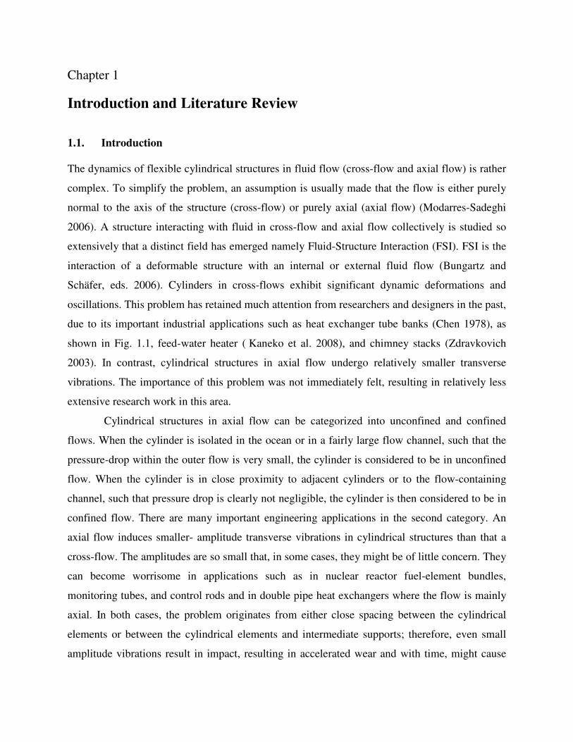
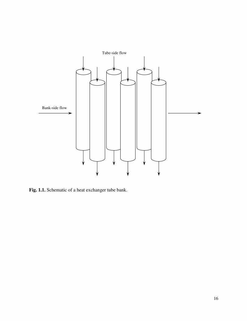
due to its important industrial applications such as heat exchanger tube banks (Chen 1978), as
shown in Fig. 1.1, feed-water heater ( Kaneko et al. 2008), and chimney stacks (Zdravkovich
2003). In contrast, cylindrical structures in axial flow undergo relatively smaller transverse
vibrations. The importance of this problem was not immediately felt, resulting in relatively less
extensive research work in this area.
Cylindrical structures in axial flow can be categorized into unconfined and confined
flows. When the cylinder is isolated in the ocean or in a fairly large flow channel, such that the
pressure-drop within the outer flow is very small, the cylinder is considered to be in unconfined
flow. When the cylinder is in close proximity to adjacent cylinders or to the flow-containing
channel, such that pressure drop is clearly not negligible, the cylinder is then considered to be in
confined flow. There are many important engineering applications in the second category. An
axial flow induces smaller- amplitude transverse vibrations in cylindrical structures than that a
cross-flow. The amplitudes are so small that, in some cases, they might be of little concern. They
can become worrisome in applications such as in nuclear reactor fuel-element bundles,
monitoring tubes, and control rods and in double pipe heat exchangers where the flow is mainly
axial. In both cases, the problem originates from either close spacing between the cylindrical
elements or between the cylindrical elements and intermediate supports; therefore, even small
amplitude vibrations result in impact, resulting in accelerated wear and with time, might cause
2
the rupture of the cylindrical elements (Paїdoussis 2004). Thus, unlike cross-flow-induced
vibration problems, low-amplitude axial-flow-induced vibration problems usually become
prominent after long period of time, causing fatigue and cracking due to cyclic stresses. Another
important reason for interest in axial-flow-induced vibration is that some systems are inherently
very flexible because of their material, support configuration, or length. These systems are prone
to larger amplitude vibrations (Paїdoussis 2004). According to Paїdoussis (2004), most of the
interest as early as 1958 in the low amplitude vibration of cylindrical structures in axial flow was
directly related to the power industry and related work was carried out for one of the following
reasons: (a) measurement of the amplitude of vibration of particular cylindrical structure
configurations, e.g., modeling nuclear reactor components such as fuel rods, monitoring tubes,
and tubular cylindrical elements in the steam generator and the flow conditions; (b)
comprehending the reasons of vibration; (c) development of mechanisms for foreseeing the
vibration amplitudes.
One of the practical examples of cylindrical structures in axial flow is seismic receiver
arrays. Seismic sonars are often used to survey the undersea geological deposits such as oil and
gas below the seafloor. Sound pulses generated from a sonar transmitter attached to a vessel
travel through the water and into the see bed. The reflected pulses are recorded by the seismic
receiver arrays also attached to the same vessel. These seismic arrays are extremely long,
neutrally buoyant, and slightly submerged in water (Paїdoussis 2004). The reflected pulses are
then analyzed to detect the presence of any mineral deposits lying under the sea floor (AML
Oceanographic 2013). In order for the system to work effectively, the dynamical behaviour of
the slender cylinder-like arrays in the water needs to be understood.
Another practical application, in biomedical science, is ‘catheterization’. This technique
is used to open a blocked or narrowed coronary artery due to substantial buildup of fatty matter.
A long narrow flexible guide wire called a ‘catheter’, equipped with a small deflated balloon and
a stent (a stainless steel mesh tube), is inserted into the artery and reaches where blockage has
occurred. The balloon is then inflated and it fixes the stent to keep the artery open. Another way
of widening the artery passage is by using a balloon catheter. A deflated balloon on a catheter is
passed into the narrowed locations and then inflated to a fixed size. The balloon crushes the fatty
deposits, opening up the blood vessel to improve flow; the balloon is then collapsed and
withdrawn (Morgan and Walser 2010). Dynamic instability of catheters can become substantially
3
critical for the successful completion of the above mentioned procedures and patient health
recovery. The instability in terms of dynamic buckling or whipping action of the catheter is one
of the reasons for coronary or vascular perforation that may lead to severe complications or even
death. It has been reported as a result of the study taken place in Columbia University where,
between April 2004 and October 2008, 13,466 angioplasties were performed and out of these, 33
(0.245%) coronary perforation cases were documented with 26 (78.8%) angiographically severe
cases. Among the fifteen patients who were treated using a single catheter, there were three
deaths (20%), two surgical explorations (13.3%), eight emergent pericardiocenthesis (53.3%),
and one event of severe anoxic brain damage (6.7%) (Ben-Gal et al. 2010). Therefore,
understanding the dynamics of such system becomes very important.
1.2. Literature Review
In this section, a review of the representative previous studies on the system of a slender cylinder
subjected to axial flow will be presented, starting from the studies done on unconfined flow,
followed by studies on confined flow.
1.2.1. Experimental Studies on Slender Flexible Cylinders in Axial Flow
One of the early experimental studies on the dynamics of slender flexible cylinders in unconfined
axial flow was conducted by Paїdoussis (1966b). He conducted experiments on horizontally
positioned cantilevered and simply supported cylinders in axial water flow. To remind the
reader, cantilevered cylinder has one of its ends clamped/fixed while the other end is free.
Simply supported cylinder has both its ends pinned to a rigid support. He fixed a smoothly
tapered rigid end-piece at the free downstream end of the cantilevered cylinder, whereas made
both the ends of the simply supported cylinder tapered over a very short distance. The
experiments served as a means to compare and validate the theoretical model of similar system
also developed by him (1966a). Paїdoussis et al. (1980b) examined, experimentally, the
dynamical behaviour of the flexible slender cylinder in axial flow, perturbed harmonically in
time. They compared the experimental results with those of theory (Paїdoussis et al. 1980a) and
found good agreement between them.
4
For solitary cylinder, Paїdoussis and Pettigrew (1979) conducted experiments to study the
dynamics of flexible cylinder in an axisymmetric confined axial fluid and two-phase flows. They
also compared the results qualitatively and quantitatively with theoretical predictions and found
that the agreement was qualitatively good and quantitatively fair. Later, Gagnon and Paїdoussis
(1994b) studied, experimentally, the coupling characteristics of cluster of cylinders clamped at
both ends in turbulent axial flow. Two, four, and twenty eight cylinder clusters were used for the
experiments with a maximum of four flexible instrumented cylinders in the cluster. The rest of
the cylinders were rigid. They recorded the vibration amplitudes of the cylinders in two
orthogonal directions. They presented the results for the clusters in the form of Power Spectral
Density (PSD), coherence plots, and inter-cylinder phases. They also conducted experiments on
four-cylinder cluster to see the effect of inter-cylinder gap. They used the experimental results to
support the theory for similar system developed by them (1994a).
1.2.2. Theoretical Studies on Slender Flexible Cylinders in Axial Flow
1.2.2.1.Linear Models
One of the earliest studies on the dynamics of slender flexible structures in axial flow was
undertaken by Hawthorne (1961). He reported the designing, fabrication, and experimental
testing of many designs of towed flexible barge all made of flexible material. Dracone is a
slender flexible container towed behind a small ship, used to transport lighter-than-sea-water
liquids such as gasoline, kerosene, and fresh water. After delivery of the cargo, the Dracone is
either rolled and carried on the ship or filled with air and towed back to land (Paїdoussis 2004).
He was concerned with the directional stability of the towed Dracone system in order to avoid
excessive stresses that might develop while towing the system in water.
Following Hawthorne’s work on towed flexible structures, Paїdoussis (1966a) studied the
dynamics of slender flexible cylinders in unconfined axial flow. This was a two-part study
comprising of (i) the development of linear analytical model of the flexible cylinder dynamics
for different boundary conditions and (ii) experiments to compare and validate the theory. The
experimental part is described in Section 1.2.1. The boundary conditions considered for the
cylinder were either clamped or pinned at both ends of the cylinder, or clamped at the upstream
end and free at the other end. The two-dimensional linear model accounted for small, free, lateral
5
motions of the cylinder immersed in fluid flowing parallel to the axis of the cylinder. He did not
account for the damping in the material of the cylinder. He used the standard boundary
conditions for the cylinder supported at both ends. However, in case of the free downstream end,
he considered a rigid end-piece at the free end the cross-sectional area of which was assumed to
be tapered smoothly to zero over a short distance such that l/L << 1. Here, L is the total length of
the cylinder including the end-piece and l is the length of the end-piece. He applied the time- and
velocity-dependent boundary condition at this free end. He observed that the inviscid force
contributed considerably in the cylinder response.
This study, however, contained an error in completely specifying the forces causing the
vibration in the cylinder. The error arose due to the absence of the term FL (∂y/∂x) in the y-
direction (transverse direction) force balance equation. This error was carried forward,
undetected, to others’ work, for example, Ortloff & Ives (1969), Pao (1970), and Chen &
Wambsganss (1972). The model itself was later extended and corrected, leading to the most
complete linear model of Paїdoussis (1973). Furthermore, a linear analytical model pertaining to
the case of a cluster of cylinders or a solitary cylinder in confined flow was also developed in
this work. The model took gravity and pressurization into account, and determined the frictional
forces in a systematic way.
Later, Paїdoussis (1974) studied the small amplitude vibration, termed sub-critical
vibration, induced in cylindrical structures by turbulence in the axial flow. Sub-critical vibrations
are small amplitude vibrations occurring at flow velocities lower than the critical flow velocities
at which fluid-elastic instabilities develop in the cylinder. Considering the range of axial flow
velocities pertaining to most industrial systems, the vibration amplitudes were small. In this
work, based on the theory developed for cylindrical structures in axial flow (Paїdoussis 1973), he
developed an analytical model to predict the dynamics of slender flexible cylinder in unconfined
and confined axial flows. Furthermore, he derived an empirical relation to predict the sub-critical
vibration amplitudes. He also explained the mechanisms of sub-critical vibrations in the
cylindrical system. He categorized the sub-critical vibrations as forced, parametric, or self-
excited. He also discussed other analytical models developed by other researchers such as
Quinn’s (1962) self-excited vibration model, Reavis’s (1969) and Chen & Wambsganss’s (1972)
forced-vibration models, Gorman’s (1969, 1971) two-phase flow forced-vibration model, and
Chen’s (1970a,b) parametric vibration model. Hannoyer and Paїdoussis (1978) examined the
6
dynamics and stability of cylindrical tubular beams conveying fluid and simultaneously
subjected to axial external flow by deriving and solving the equation of motion while taking into
account the boundary-layer thickness on the cylinder due to the external flow, internal
dissipation, and gravity effects. They also conducted experiments on similar system in order to
support the theoretical predictions.
Paїdoussis et al. (1980a) investigated, theoretically, the dynamical behaviour of a solitary
flexible slender cylinder in pulsating flow. They first conducted the theoretical analysis of the
system in steady and unperturbed flow for various sets of boundary conditions, and established
(i) the eigenfrequencies of the system at any given flow velocity and (ii) the critical flow
velocities that mark the onset of system instabilities. Then they did the analysis of the system in
pulsating flow, establishing the existence of parametric resonances. They also looked into the
effects of the mean flow velocity, boundary conditions, dissipative forces, and virtual
(hydrodynamic) mass on the extent and location of the parametric instability zones. Paїdoussis
(1983) reviewed the two classes of flow-induced vibrations encountered in nuclear reactors and
reactor peripherals, vibration of cylindrical structures induced by cross-flow and by axial flow.
In view of the importance of safety for reactor plant in order to safeguard the potentially very
delicate environment and people, this study highlighted the potential causes of reactor damage
due to flow-induced vibrations and their underlying mechanisms. The review encompassed
buffeting, often referred to as subcritical vibration, in a solitary cylinder subjected to axial flow,
flow periodicity, as well as fluid-elastic instabilities in cylinder also subjected to axial flow.
De Langre et al. (2007) investigated the effect of length on long flexible cylinders in axial
flow. Following Paїdoussis (1973) and Paїdoussis et al. (2002), they modelled the cylinder as
beam. They proposed a new dimensionless form of the equation of motion governing lateral
vibrations to make it appropriate for the analysis of the effect of the length. They also found a
limit regime where the length of the cylinder did not affect the characteristics of the instability
and the deformation was confined to a finite region close to the downstream end. Wang and Ni
(2009) reviewed the linear dynamics of different flexible structures as a result of interaction with
fluid flow. They considered the fundamental case scenarios of the fluid-induced instabilities in
structures such as straight pipes conveying fluid, nano-tubes conveying fluid, tubular beams
subjected to both internal and external axial flows, cylindrical shells subjected to axial flow,
plates in axial flow, and slender structures in axial flow or axially towed in quiescent fluid.
7
Considerable work has been done on the dynamics of clusters of flexible cylinders in
axial flow and solitary cylinder in annular axial flow; both are cases of confined flow. One early
study is by Paїdoussis (1979). A linear theory of the dynamics of clusters of independently
supported flexible cylinders in axial flow was developed and an extensive discussion of the
behaviour of such systems with increasing flow velocity was presented, with emphasis on the
modal forms of free coupled motions of the cylinders and on the onset of the instabilities. Results
of an experimental study, involving systems of two, three, or four cylinders with different inter-
cylinder gaps and support conditions were also presented and compared with theoretical results.
Related to the earlier work, Paїdoussis et al. (1983a, b) in a two part study analyzed the dynamics
of a cluster of three structurally interconnected cylinders in vacuum in part 1. The
interconnection was modeled through translational and rotational linear springs. The knowledge
and experience gained in the first part was later utilized to analyze the dynamics of the same
system in axial flow.
Paїdoussis (1993) delivered the Calvin Rice lecture in which he covered the topics of the
stability of pipes conveying fluid and of cylinders in axial flow. He mentioned that although
much of the research work on these topics is curiosity driven and little or no application was in
mind, unexpected uses and applications materialized in the following years. He indicated that the
applications ranged from a marine propulsion system to the dynamics of deep water risers. He
described the dynamics of thin pipes (shells), cantilevered pipes, and pipes with supported ends
conveying fluid, and cylinders and shells in axial flow and leakage flow. Later on, Gagnon and
Paїdoussis (1994a) developed a random vibration theory to study the fluid coupling
characteristics and turbulence-induced response of a four-cylinder cluster system. The work was
motivated by the practical application in nuclear power plants in which vibration may be induced
by the axial flow in the nuclear fuel elements stacked in a cluster leading to serious
consequences. They developed the random vibration theory based on the work of Reavis (1967,
1969) and Paїdoussis and Curling (1985). They also used the updated form of the mean flow
theory developed by Paїdoussis and Suss (1977). The mean flow theory provides the free-
vibration lateral deflection characteristics of cluster of cylinders subjected to steady axial flow.
In the same work, they combined both the theories (random vibration theory and mean flow
theory) into a global multi-degree of freedom random vibration model. The distinguishing
features of this model are the capability of predicting the response of the mixed rigid-flexible
8
cylinders cluster, changing frequencies, and modal characteristics with varying mean flow
velocity.
Concerning fluid-elastic vibration, Paїdoussis (1981) presented a critical assessment of
the state-of-the-art for flow induced vibrations of cylinder arrays in cross and axial flows. He
discussed different mechanisms that were recognized previously as potentially capable of giving
rise to vibrations in cross and axial flows including small-amplitude vibrations induced in
cylinder arrays in axial flow. He presented an empirical relation governing the forced vibrations
in axial flow and discussed the underlying mechanisms of forced vibration, hydrodynamic
coupling, parametric resonances, and fluid-elastic instabilities in cylinder arrays also in axial
flow.
Considerable work has been done on the dynamics of rigid cylindrical structures in
unsteady flows inside narrow annuli. For brevity, only some representative studies are
mentioned. Mateescu and Paїdoussis (1985) studied, analytically, the effect of unsteady potential
flow in an axially variable annulus on the dynamics of oscillating rigid center-body. They
extended the model to make it compatible with short center-body as well. Later, Mateescu and
Paїdoussis (1987) investigated the unsteady viscous effects on the annular-flow-induced
instabilities of a rigid cylindrical body oscillating about a hinge in a coaxial narrow duct. For
that, they extended the previously developed analytical model by Mateescu and Paїdoussis
(1985) to account for the unsteady viscous effects of a fluid flow in an approximate manner.
They also compared the inviscid and viscous flow theories. Extending the formulation to flexible
structures, the dynamics and stability of a flexible cylinder in annular flow was studied by
Paїdoussis et al. (1990). The principal contribution of this work was that firstly, they formulated
the inviscid forces based on the potential flow theory and secondly, they formulated the unsteady
viscous forces not by an adaptation of Taylor’s expression but by a systematic application of the
Navier-Stokes equations. They modified the linear model for a slender flexible cylinder in axial
flow developed by Paїdoussis (1973) to make it work for the flexible cylinder in annular flows
subjected to unsteady viscous fluid forces by substituting the formulated inviscid and viscous
force terms in the equation of motion. They also obtained the results for very narrow annuli.
There is a fair amount of research work on the dynamics of continuous flexible
axisymmetric bodies in axial leakage flow. To remind the reader, when the fluid gap or annulus
is narrow, the flow is considered to be a leakage flow. Fujita and Shintani (1999, 2001) studied
9
the flow-induced vibration instability of a long flexible axisymmetric rod due to axial leakage
flow for different end boundary conditions. Unlike considering the axisymmetric rod as a rigid
body and not a continuous body as in the previous studies, they considered the rod as a
continuous flexible body. They analytically coupled the equations for the fluid and the structure.
In the derivation of the analytical model, they obtained the expressions for the added mass,
added damping, and added stiffness by considering unsteady pressure acting on the rod. They
simplified the derived linear equation of motion into matrix form and then solved in MATLAB
to obtain the complex eigenvalues. As a continuation of their work, Fujita et al. (2007) conducted
experiments on a simply supported axisymmetric circular elastic beam subjected to laminar axial
leakage flow. They also derived and analytically solved the coupled equations for similar system
of fluid and beam structure for verification. They presented the analytical results in the form of
complex eigenvalues. They, specifically, focused on explaining the generation of travelling
waves and the energy balance for the distortion of vibration response in axial direction of the
system at the transition from a lower predominant frequency to a higher one by means of
experimental and analytical results. Later, Langthjem et al. (2006) bridged and extended the
models developed by Li et al. (2002) and Fujita and Shintani (2001) to account for an eccentric
simply supported flexible cylindrical rod undergoing static and dynamics instabilities due to
annular laminar or turbulent leakage flow. For this, they derived the coupled fluid-structure
equations and then discretized the equations using the Bubnov-Galerkin finite element method
(Cook et al. 1989). They chose this discretization method because of its capability to handle
various end boundary conditions and asymmetries in a very simple way by choosing the
expansion functions ‘once and for all’. Finally, they grouped the coupled equations into single
matrix system and simplified it to ‘extended’ eigenvalue problem. The results they obtained were
in the form of complex eigenvalues. Langthjem and Nakamura (2007) investigated the effect of
swirl on the stability of slender flexible rod in axial annular leakage flow. They derived the
analytical relations and analyzed the results. For the derivations, they assumed laminar fluid flow
and vibrations of the rod in one plane. More recently, Fujita and Ohkuma (2010) used the already
proposed analytical model by Fujuta and Shintani (2001) to investigate how the critical flow
velocities for divergence and flutter vary for different end boundary conditions of an elastic
beam in a narrow axial flow. They also conducted parametric studies of the effects of fluid
10
temperature, width of annular gap, viscosity of fluid, and structural damping on the critical flow
velocities.
Some studies have specifically focused on the fundamental mechanisms and practical
aspects of flow-induced instabilities of flexible structures in unconfined and confined flows
together. In order to present the consequences of such instabilities, Paїdoussis (1980) compiled
many practical cases of flow-induced vibration problems in heat exchangers and nuclear
reactors. Later, Paїdoussis (1987) presented an abridged state-of-the-art review paper on flow-
induced instabilities of cylindrical structures for the Fluid-Structure Interaction (FSI) categories
mentioned above. This paper provides a brief and somewhat unified discussion of the subject
matter. Naudascher and Rockwell (1990) also discussed, very briefly, the dynamics of slender
bodies in axial flow pertaining to a rod (they referred to the flexible cylinder as a rod) in external
axial flow, leakage flow, and multiple bodies in axial flow. They described the effect of
confinement in case of multiple cylinders in an array on critical velocities. A more recent paper
by Paїdoussis (2008) discussed how the experience gained in studying the problem of pipes
conveying fluid radiated into other areas of Applied Mechanics, particularly other problems in
FSI involving slender structures and axial flows; specifically the dynamics of (a) Pipes
conveying fluids; (b) slender cylinders in unconfined and confined axial flows; (c) cylindrical
shells subjected to axial flow; and (e) plates in axial flow. It also provided a recap of equations
and brief insight into the instability mechanisms in such problems.
1.2.2.2.Nonlinear Models
Through a linear model of a flexible cylindrical system in axial flow, one can reliably predict the
occurrence of first instability, which is in most of the cases static often referred to as divergence,
but post-divergence dynamics of the system needs to be validated through a nonlinear model
(Paїdoussis 1998, 2004; Modarres-Sadeghi 2006). This was done in 2002 when the first
complete two-dimensional nonlinear analytical model governing the dynamics of cantilevered
inextensible flexible cylinders in unconfined axial flow was developed. This work was a three-
part study comprising (i) the physical dynamics (Paїdoussis et al. 2002), (ii) the nonlinear
equations of motion (Lopes et al. 2002), and (iii) the nonlinear dynamics (Semler et al. 2002). In
first part, the physical dynamics of the system via experimental behaviour of elastomer cylinders
in water flow and the energy transfer mechanisms were examined from a work-energy
11
perspective without obtaining the solution of the equations of motion. They experimentally
determined the critical flow velocities for the onset of static and dynamic instabilities in a
vertical flexible cantilevered cylinder enclosed in a relatively wider channel with axial flow and
studied the effects of free-end shape, mass ratio, and surface roughness and slenderness on these
critical velocities. In the second part, the nonlinear equation of motion was derived for the
dynamics of a slender cantilevered cylinder in axial flow terminated by an ogival free end. In
third part, the dynamics of the cantilevered cylinder in axial flow were explored by means of the
equations of motion derived in part 2, and using the Finite Difference Method (FDM) and AUTO
(a bifurcation software package) as numerical tools in order to obtain the solution of the
discretized equations.
Modarres-Sadeghi et al. (2005) developed weakly nonlinear equations of motion for an
extensible slender flexible cylinder with extensible centreline subjected to axial flow. They
considered simply supported boundary conditions of the cylinder. The model comprised two
coupled nonlinear equations describing the motions involving the longitudinal and transverse
displacements. The derivation of the equations of motion was carried out in a Lagrangian
framework. The equations were later transformed into a set of second-order ordinary differential
equations using the Galerkin technique, which were finally solved numerically using Houbolt’s
finite difference method. The authors also analyzed the influences of frictional coefficients,
externally imposed uniform tension, and dimensionless axial flexibility on stability and
amplitude of the buckled solution. Later, Modarres-Sadeghi et al. (2007) presented a
comparative study of the dynamics of a cylinder with simply supported and clamped-clamped
(both the cylinder ends clamped) boundary conditions. Houbolt’s Finite Difference Method
(FDM) and AUTO were used to solve the equations of motion. With the combination of these
methods, they could obtain the bifurcation diagrams and dynamic response of the cylinder over a
wide range of flow velocity.
1.3. Motivation of Present Work
A comprehensive literature review indicates that earlier experiments on systems similar to the
present one were conducted with different objectives in mind. For example, the experiments
conducted by Paїdoussis (1966b) were focused on studying the two-dimensional dynamics of a
horizontal cylinder subjected to axial flow in order to validate and support the two-dimensional
12
linear theory of similar system developed by him (1966a). Other set of experiments conducted by
Paїdoussis et al. (1980b) were focused on studying the effect of harmonically perturbed axial
flow pulsation frequency and amplitude on the parametric resonance oscillations in solitary
cylinder clamped at its both ends. They used shorter and thinner cylindrical system than the one
used in the present experimental study. Later, the experiments conducted by Paїdoussis et al.
(2002) on the vertical cantilevered cylinder in axial flow were intended to compare the
experimental results with those of the two-dimensional nonlinear theory for similar system
developed by them (Lopes et al. 2002). Hence the need remains to conduct the experiments on
solitary cantilevered cylinder in axial flow to study the three-dimensional dynamics of the
cylinder by determining the critical flow velocities, cylinder displacements and oscillation
amplitudes, oscillation frequencies, and path traced by the oscillating cylinder, and also to
validate and complement the three-dimensional nonlinear model results for similar system. The
present experiments are also going to serve as a validation tool for the presently used two-
dimensional linear and nonlinear models to study the dynamics of the same system.
In fluid-structure interaction problems, a precise calculation of the force coefficients such
as longitudinal and normal viscous coefficients, base drag coefficient, and zero-flow normal
force coefficient present in the equations of motion associated to the fluid forces acting on the
cylinder surface is imperative. In the previous theoretical studies on cylindrical system in axial
flow with different support boundary conditions (Paїdoussis 1966a, 1973; Paїdoussis et al.
1980a; De Langre et al. 2007), the force coefficients especially the viscous force coefficients in
transverse and longitudinal directions were considered to be equal. Therefore, these force
coefficients are calculated based on the parameters actually used in the experiments and
theoretical models. It is expected that the implementation of these calculated coefficients in the
linear model will enable the model to better predict the dynamics of the system.
As indicated earlier, a linear model can reliably predict the first point of instability of a
flexible system in axial flow, which is most of the time a static instability commonly referred to
as divergence. The dynamics of the system thereafter has to be verified via a nonlinear model
(Paїdoussis 1998, 2004; Modarres-Sadeghi 2006). From the literature review, it is noted that in
the research work utilizing the nonlinear models to describe the system dynamics of a slender
flexible system in axial flow (Paїdoussis et al. 2002; Modarres-Sadeghi 2005, 2007), the force
coefficients were either selected within a reasonable range or obtained based on some simple
13
relations. Therefore, an effort is undertaken to solve the nonlinear equation with the presently
calculated force coefficients incorporated in it in order to better describe the nonlinear dynamics
of the system.
Finally, a comprehensive literature review indicates that a three-dimensional coupled
nonlinear model that governs the dynamics of cylindrical structures in axial flow has not yet
been developed and studied. This, despite the fact that, in one of the aforementioned experiments
(Paїdoussis et al. 2002), three-dimensional dynamical behaviour was observed. In fact the path
traced by the end of the cylinder was observed to be orbital. Lack of knowledge to account for
the three-dimensional behaviour especially the non-symmetry found in the cylinder motion,
important in the above-mentioned practical applications, is the motivation behind the present
work, which is aimed at developing a three-dimensional coupled nonlinear model for a confined
flexible cylindrical structure in axial flow in a Finite Element Method (FEM) based modelling
and simulation package called ADINA in addition to experiments and other theoretical work
done.
1.4. Objectives
The objectives, therefore, are to conduct experiments on a slender flexible cantilevered cylinder
in axial flow, obtain and incorporate the presently calculated fluid force coefficients in the two-
dimensional linear and nonlinear analytical models to study the linear and nonlinear dynamics of
a cantilevered cylinder for a flow velocity range, investigate the effect of confinement on the
dynamics of cylinder, develop three-dimensional nonlinear cantilevered cylinder model in
ADINA, a specialized finite element modeling and simulation package, and investigate its
response for a flow velocity range. The theoretical (linear and nonlinear) and numerical (created
in ADINA) models are going to be validated with the help of experimental results. Finally, the
results of the models are going to be compared together and presented at one place in order to
observe the coherence of the results of the models and also to build a degree of confidence up to
what beam mode, each model is capable of predicting the dynamics of the system.
14
1.5. Outline of the Thesis
In Chapter 1, a brief introduction of the subject area, its practical applications, and motivation
behind the present work are given. In addition, a review of the previous studies on the dynamics
of slender flexible structures in axial flow is also presented. This review includes earlier
analytical and numerical studies on flexible cylinders in axial flow using linear and nonlinear
models, for the cylinder in wide and narrow channels. It also includes the experimental studies
done so far on similar systems. Finally, the objectives of the present study are presented.
In Chapter 2, procedures to calibrate the non-contacting laser-optical tracking systems
used to measure the cylinder displacements and determine the essential parameters such as
flexural rigidity, EI, logarithmic decrements, δn, hysteretic damping constant, , and the
dimensionless viscoelastic damping constant, of the cylinder are presented. Then the fluid
flow velocity profile inside the water tunnel test-section is also determined with the help of Laser
Doppler anemometry (LDA). This chapter also includes descriptions of the LDA equipment and
the experimental set-up to obtain these measurements. Description of the experimental set-up for
the cantilevered cylinder with ogival end piece inside the vertical transparent test section of a
water tunnel is then presented. Finally, the experimental results and quantitative analysis are
presented.
In Chapter 3, the linear equation of motion of the flexible cylinder is considered. The
linear partial differential equation is discretized by using the ‘extended Galerkin method’,
resulting in a set of ordinary differential equations, solving them through a MATLAB code, and
analyzing the results. The fluid forces such as inviscid forces, viscous forces, and hydrostatic or
pressure forces acting on the surface of the cylinder contribute to the overall dynamics of the
cylinder. Therefore, the coefficients associated to the viscous fluid forces such as longitudinal
and normal viscous coefficients, base drag coefficient, and zero-flow normal coefficient are
recalculated and incorporated in the linear model and the model is then solved to yield the
dynamical behaviour of the cylinder with increasing flow velocities.
In Chapter 4, nonlinear equations of motion are solved using Houbolt’s Finite Difference
Method (FDM) and the results employing the previously used coefficients by Semler et al.
(2002) and the presently calculated ones are presented. Bifurcation diagrams, time histories, Fast
Fourier Transform, Power Spectral Density, phase plots, Poincaré map, and mode shapes are
*µ
*α
15
obtained to analyze the cylinder dynamics with increasing flow velocity. Finally, comparisons of
the results in terms of the critical velocities for instabilities reported by Semler et al. (2002) and
present model with previous and present force coefficients are presented.
In Chapter 5, the results of a three-dimensional model of a flexible cylinder enclosed in a
channel created via a commercially available finite element modeling and simulation package,
namely ADINA are presented. The simulations are performed at different water and air flow
velocities and the vibration response of the cylinder is obtained. Finally, water and air flow
results in terms of critical velocities marking the instabilities of the cylindrical system are
compared.
In Chapter 6, the results in terms of the critical velocities, displacement magnitudes, and
frequencies of linear and nonlinear models, experiments, and numerical model in water and air
flows using the previous and present force coefficients are compared.
Finally Chapter 7 summarizes the thesis with the conclusions of the research work
undertaken and suggestions for future work.
16
Fig. 1.1. Schematic of a heat exchanger tube bank.
Bank-side flow
Tube-side flow
Chapter 2
Experiments on Cantilevered Cylinder in Axial Flow
2.1. Introduction
As indicated in Chapter 1, earlier experiments on systems similar to the present one were
conducted with different objectives in mind. The experiments conducted by Paїdoussis (1966b)
were focused on studying the two-dimensional dynamics of a horizontal cylinder subjected to
axial flow in order to validate and support the two-dimensional linear theory of similar system
developed by him (1966a). Using similar system to the 1966 experiments, Paїdoussis et al.
(2002) conducted experiments this time on a vertical cylinder in order to compare the
experimental results with those of the two-dimensional nonlinear theory for similar system
developed by them (Lopes et al. 2002). Other set of experiments conducted by Paїdoussis et al.
(1980b) were focused on studying the effect of harmonically perturbed axial flow on the
parametric resonance oscillations in solitary cylinder. From the review of early experimental
work, a need is felt to conduct experiments on the cantilevered cylindrical system in axial flow in
order to study its three-dimensional dynamics and also to validate and complement the three-
dimensional nonlinear numerical model results of similar system. The present experiments are
also intended to compare the presently used two-dimensional linear and nonlinear models for
their efficacy in predicting the dynamics of similar system.
This chapter gives an account of the experiments conducted on vertical flexible
cantilevered cylinders in axial flow. The elastomer cylinder is made of Silastic® E RTV Silicone
Rubber from Dow Corning. The cylinder casting is done using a two-part silicone rubber kit
consisting of a base and a curing agent. The procedure is described by Paїdoussis (1998) and
Rinaldi (2009). Although they have given the procedure for a pipe, it is similar for cylinder. The
only difference is that the mould for cylinder is of different length and diameter, and does not
have the central rod, which is meant to make a hollow cylinder (i.e., a pipe) for internal axial
flow. The upstream end of the cylinder is clamped and supported by four arms, which are
rounded at the leading edge and pointed at the trailing edge as shown in Fig. 2.1 (a). The
downstream free end of the cylinder is terminated by an ogival rigid end-piece as shown in Fig.
2.1 (b). The cylinder centreline is considered to be inextensible. The entire cylinder assembly is
18
enclosed in a vertical transparent plexiglas test-section of a closed loop water tunnel as shown in
Fig. 2.2. The flow direction of the water inside the test-section is downwards. The objective of
the experiments is to study the dynamics of the flexible cantilevered cylinder by determining the
critical velocities for static and dynamic instabilities, as well as the effect of flow velocity on the
amplitudes and frequencies of the unstable cylinder.
This chapter also includes the procedures to determine the structural and damping
constants of the cylinder, calibrate the flow velocity and non-contacting one-dimensional optical
displacement sensors used to record the cylinder motions, obtain the velocity flow profile inside
the test-section, and the profile of the path traced by the oscillating cylinder.
2.2. Physical Description
The cantilevered cylinder has length, L = 0.5265 m, diameter, D = 0.0254 m, end-piece length, l
= 0.0346 m, and tapering end-piece shape factor estimated to be f = 0.8 (see Appendix A). The
vertical test-section (‘channel’), made of plexiglas, has length, Lch = 0.77 m and diameter, Dch =
0.203 m. The confinement factor, χ is a measure of the confinement of a cylinder inside a
channel or its proximity to the surrounding cylinders. It is defined by the expression (Paїdoussis
2004)
.22
22
−
+=
DD
DD
ch
chχ (2.1)
Its value approaches 1 for a cylinder in unconfined flow and increases as the cylinder
confinement is increased. Its value as calculated is 1.03. Water is circulated in the water tunnel
by an Ingersoll-Rand type S horizontal split-case centrifugal pump with a discharge capacity of
2,200 gallons per minute. The maximum flow velocity achieved in the water tunnel is about 5.5
m/s corresponding to u = 8.2.
2.3. Calibrations of Laser-Optical Sensors
Two laser sensors have been utilized in the experiments. Therefore, before the experiment,
calibrating both sensors is necessary. One is a Micro-Epsilon OptoNCDT 1400-200 non-
contacting laser-optical displacement measurement sensor and the other is MEL M27L non-
19
contacting laser distance sensor. The calibration of these laser sensors enable the output voltages
from the sensors to be converted to linear distances. The laser heads of both sensors are placed at
a known distance, x, from some reference, say a rigid vertical plate. The laser heads are then
moved gradually with known increments, ∆x, towards the reference. At each location of the laser
head, the DC voltage is recorded by a multimeter. The known distances, x1, x2, x3, ……, xn are
then plotted against the output voltage for each sensor as shown in Figs. 2.3 and 2.4. Each of the
figures shows that the output voltage varies linearly with the distance. The goodness of fit 2fitR
for Figs. 2.3 and 2.4 come out to be 1 and 0.9998, respectively.
2.4. Flexural Rigidity of Cylinder
One of the essential quantities to know is the flexural rigidity of the cylinder, EI. The most
convenient method to determine EI is by conducting planar free vibration experiments of a
cantilevered cylinder hung vertically in air and excited in its first mode natural frequency. This
can be achieved rather effortlessly by displacing and releasing the free end of the cylinder such
that it oscillates in its first mode. The displacement of the cylinder is then measured using the
Micro-Epsilon OptoNCDT 1400-200 non-contacting laser-optical displacement measurement
sensor, which lies in the plane of oscillation, giving the output as a voltage. The resulting time
signal is post-processed in a customized MATLAB code to obtain the Fast Fourier Transform
(FFT) and Power Spectral Density (PSD) plots as shown in Fig. 2.5. FFT is an efficient
algorithm to transform a discrete signal such as displacements of a structure in time domain into
its discrete frequency domain (Strang 1994). PSD is a measure of the distribution of the power of
a signal over the different frequencies (Miller and Childers 2004). From these plots, the first
mode natural frequency, f1, is determined, which is 1.10 Hz. It is known that both the frequency
and flexural rigidity depend on the gravity parameter, γ. Therefore, the expression given by
Paїdoussis and Des Trois Maisons (1969),
( )[ ] ( )[ ],
ReRe2
1
2
1 effL
g
Ω=
ω
γ (2.2)
is used. Here, Re (ω1) is the real part of dimensionless first mode natural frequency, g is the
gravitational constant, Leff is the effective length of cylinder, and Ω1 = 2πf1 is the dimensional
20
first mode natural frequency in rad/s. Substituting the values of the parameters on right hand side
of eq. (2.2) and using Table A.1 from Paїdoussis and Des Trois Maisons (1969), the
corresponding value of γ is found by linear interpolation. EI is then calculated from the
expression
EI
mgL3
=γ , (2.3)
given by Paїdoussis and Des Trois Maisons (1971). Here, m is the mass of the cylinder per unit
length. Equation (2.3) thus gives the value of EI = 0.0719 N.m2.
2.5. Logarithmic Decrements
The logarithmic decrements, δn, of the cantilevered cylinder in its first three modes are also
determined experimentally by planar free vibrations of the cylinder hung in air and excited in its
first, second and third modes. The first mode is, once again, excited manually, i.e., by displacing
the free end of the cylinder in the plane of the measuring laser sensor. However, the second and
third modes are excited mechanically with the help of a crank-slider mechanism. This
mechanism consists of a DC motor attached to a rod through a crank that enables the rod to slide
to and fro as shown in Fig. 2.6. The digital controller is used to control the r.p.m. of the motor,
exciting the cylinder in the second and third modes.
When the DC motor is stopped abruptly, the cylinder oscillates, for a time, in only the
desired mode. The decaying oscillations in the first, second and third modes are then recorded
one by one with the help of the laser sensor. A MATLAB code with low-band, pass-band, and
high-band Chebyshev type 1 filters of order 5 for first, second, and third mode cylinder
oscillations, respectively, is used. Filters are used in order to remove any unwanted components,
such as noise, from the signal. Figures 2.7 and 2.8 show the time histories, FFTs, and PSDs of
the second and third modes, respectively.
The second and third mode frequencies, thus, determined are f2 = 4.52 Hz and f3 = 11.96
Hz. The filtered signal of each mode is then used to obtain natural logarithm (ln) of the cylinder
displacement and plot it against time. Figure 2.9 shows a representative plot of ln(Displacement)
versus time of the first mode. The slope of the decaying peaks of ln(Displacement) and the
frequency of each mode are substituted in the expression
21
n
nf
slope=δ (2.4)
to determine the logarithmic decrements, δn, which are δ1 = 0.021, δ2 = 0.095, and δ3 = 0.558.
The reason of δ3 being so high than δ1 and δ2 is due to system’s rapid third mode oscillation
decay.
2.6. Damping Constants
In order to consider the internal dissipation of the cylinder, a two-constant damping model is
utilized. It is necessary to determine the hysteretic damping constant, *µ ,and the viscoelastic
damping constant,*α . The expression given by Paїdoussis and Des Trois Maisons (1971), i.e.,
( )n
nn
ωαµ
δδ
Re**
*
+= (2.5)
is used. The procedure to determine the damping constants begins with determining *
nδ and Re
(ωn) for each mode. This is done by reading directly from Figs. 1 and 2 given by Paїdoussis and
Des Trois Maisons (1971) corresponding to γ calculated in Section 2.4. Substituting the known
values of *
nδ , Re (ωn), and δn for each mode in eq. (2.5) gives rise to three independent linear
equations. There are now two unknowns, i.e., *µ and *α , and three equations. From these
equations, three sets of two equations each are formed, i.e., sets of eq. (2.5) for first and second
modes, first and third modes, and second and third modes. Each set is solved simultaneously to
get *µ and*α , thus obtaining three values of each damping constant. The average of each
constant thus provides a good estimate to start fine-tuning the values and reaching values with
minimum error in computing *
1δ , *
2δ , and *
3δ from eq. (2.5) as a check. This fine-tuning is done in
MATLAB using an optimization algorithm namely “fmincon”. fmincon finds minimum of
constrained nonlinear multivariable function. It actually attempts to find a constrained minimum
of a scalar function of several variables starting at an initial estimate xo. The simplest of the
syntaxes is x = fmincon (fun, xo, A, b). The algorithm starts at xo and attempts to find a
minimizer x of the function described in fun subject to the linear inequalities A* x ≤ b. The initial
estimate xo can be a scalar, vector, or matrix. A and b are the Linear constraint matrix and its
22
corresponding vector b, respectively (MATLAB help file 2010). Finally, the values obtained are
*µ = 0.0272 and *α = 0.000378.
2.7. Flow Velocity Measurement Calibration
The water tunnel, used for the experiment, has a small bypass flow pipe for water circulation in
addition to the main flow pipe. Venturi flow meters are fitted on both pipes. There are two
differential-pressure transducers (Huba-692) across each of the Venturi meters, of which the
readings are, respectively, displayed on two controllers (ATR141, used as read-out unit); one
controller for each flow pipe. The controller ATR141 for the differential-pressure transducer
(Huba-692) connected to the Venturi flow meter on the main flow pipe and the centrifugal pump
speed in terms of r.p.m. are calibrated using a pitot-static tube and a mercury manometer. For
calibration and actual experiments, the small bypass pipe is kept closed with the help of a choke
valve and water is allowed to flow through the main pipe only. Therefore, the output panel shows
the readings of only the Venturi meter of the main pipe. The pitot-static tube is inserted through
the lower test-section window and its tip is carefully aligned with the centreline of the test
section, as shown in Fig. 2.10. Thereafter, a mercury manometer is connected to the pitot-static
tube. From the height of the mercury column, one can obtain the flow velocity using the relation,
shown by Tang (2007)
Hg
water
HgghU
−= 12
ρ
ρ, (2.6)
where, ρHg is the density of mercury, ρwater is the density of water, and hHg is the height of
mercury column.
The water tunnel is opreated from its idle state to higher flow velocities by increasing the
rotational speed of the pump by increments of 50 revolutions per minute (r.p.m.); the
corresponding values of ATR141 readings from the output panel and the height of mercury
column from the manometer being noted. Figure 2.11 shows the plot of height of mercury
column in inches versus the ATR141 readings and the linear curve fit of the data with 2fitR equal
to 0.997. The orign corresponds to U = 0 m/s, i.e., the pump being in idle state. Figure 2.12
shows the calculated flow velocity plotted against the ATR141 readings. The curve fit is via a
23
sixth order polynomial with 2fitR = 0.9988. This plot provides the calibration of the controller for
the differential pressure transducer (Huba-692). Figure 2.13 shows the linearly fit flow velocity
calibration curve for the r.p.m. of the pump with 2fitR = 0.9996.
2.8. Flow Velocity Profile inside the Test-Section
The flow velocity profile in the test-section is measured experimentally. For that, the cylinder
model and support are removed from the test-section. The water tunnel is filled with water and
operated at a target flow velocity. Since the actual experiment of studying the cylinder dynamics
is done for a velocity range mostly in the turbulent flow regime, it has been ascertained that the
velocity profile obtained experimentally is for turbulent flow. The water tunnel was operated at
mean flow velocity of 1.9 m/s for the experiment. The corresponding Reynolds number, Re and
volume flow rate are 3.842×10⁵ and 0.0627 m
3/s, respectively.
Laser Doppler Anemometry (LDA) was used for the experimental procedure. LDA, also
known as Laser Doppler velocimetry (LDV), is the technique of using the Doppler shift principle
in a laser beam to measure the velocity of fluid flow in transparent or semi-transparent channel,
or the motion of opaque or reflecting vibrating surfaces. Fluid flow measurement is undertaken
from the Doppler shift effect on a beam scattered by very small reflecting spheres, called the
seeding particles, moving within the fluid flow (Yeh and Cummins 1964). LDA passes two
beams of parallel, monochromatic, and coherent laser light crossing at a point in the flow of the
fluid being measured. These two beams are usually obtained by dividing a single beam, thus
ensuring coherence between the two lasers. Lasers with wavelengths in the visible spectrum
(390–750 nm) are usually used. A transmitting optics focuses the beams to intersect at the focal
point of the laser beams, where they interfere and generate a set of fringes. As seeding particles
moving in the fluid pass through these fringes, they reflect light that is then collected by a
receiving optics and finally focused on a photodetector. The reflected light fluctuates in intensity,
the frequency of which is corresponding to the Doppler shift between the incident and scattered
light, and is thus proportional to the component of particle velocity which lies in the plane of the
two laser beams. If the sensor is aligned to the flow in such a way that these fringes are
perpendicular to the flow direction, the electrical signal generated at the photodetector will then
be proportional to the seeding particle velocity inside the flow (Drain 1980).
24
Flowlite is an integrated laser-optics system developed by Dantec. The laser head
stimulates Helium-Neon (He-Ne) laser beam with a focal length of 0.16 m. The seeding particles
used in the flow are Iriodine 100 silver pearl having size range of 10 to 15 µm. The flowlite
system used gives one-dimensional flow velocity. It is designed for use with Dantec’s signal
processors and BSA Flow application post-processing software (Dantec Dynamics 2004). The
output data appears in the software as a histogram of flow velocity probability distribution, as
percent count. The software selects a range of flow velocity based on the data input from the
laser-optics system. The data input contains the velocity components of the seeding particles in
only the axial direction; if some particles flow at some angle to the cylinder axis, only the axial
components of their velocities is recorded. In this way, a range of axial velocities are input to the
software. These velocities are then quantized into uniform velocity ranges; each range being
confined to a histogram bar. Each histogram bar is horizontally centered on the mean value of its
velocity range. The histogram bar possessing the highest occurrences of its seeding particles’
velocities exhibits maximum percent count in the histogram and its mean velocity is considered
as the required velocity at that particular location. In other words, the flow velocity is quantized.
The higher the percent count of one particular histogram bar as compared to the others, the more
uniform is the flow. Furthermore, the larger the number of histogram bars, the more accurate is
the velocity determination. In the present measurements, a histogram resolution of 0.01 m/s,
which is 0.53 % of the mean water tunnel velocity, with 525 histogram bars is used.
The procedure starts by placing the laser head horizontally facing the test-section in such
a way that the focal point of laser beams either reaches the inside centre of the test-section or
closest to it. The data at that point is then recorded. The laser head is then moved away from the
test-section with equal increments such that the focal point of beams inside the test-section
moves towards its inner wall and data is recorded at each location. Two representative
histograms and velocity plots are shown in Figs. 2.14 and 2.15. The histograms in these figures
are not symmetric as the shape of the histogram depends on the distribution of the axial
components of seeding particles’ velocities in the histogram bars. The histogram also shows the
normal velocity distribution.
Finally, the velocity profile obtained is shown in Fig. 2.16 with 2fitR = 0.9908. The curve
is sixth order polynomial:
25
167.11035.11007.81038.2104103109 22335465767 +×+×−×+×−×+×−= yyyyyyU . The y-
axis marks the inner surface of the test-section. The solid circles represent the velocities at
different locations. A curve fit of the velocity data shows the turbulent velocity profile. The
figure also shows that there are no velocity data points at radial distances less than 0.0029 m.
The reason is that it is very difficult to measure the velocity very close to wall. Therefore, the
velocities at radial distances between 0 and 0.0029 m are resolved theoretically by the law of the
wall for turbulent flow. One of commonly used models for law of the wall is the logarithmic log
law model given as
+++ += Cyk
u ln1
, (2.7)
where, u+ is the dimensionless velocity, k is the Von Karman constant, y
+ is the dimensionless
wall coordinate, and C+ is a constant. u
+ and y
+ are given by the expressions
,*
u
uu =+ (2.8)
and
,*
k
yuy
ν=+ (2.9)
respectively. In these expressions, u is the mean flow velocity, u* is the frictional velocity, y is
the radial distance of the point, where velocity is to be determined, and νk is the kinematic
viscosity of water. The known values are k = 0.41, C+ = 5.0, and υ = 1.004×10
6 m
2/s (Schlichting
and Gersten 2000). It is known that near the wall in turbulent flow, there are two adjacent layers,
namely the inner layer and outer layer. The inner layer is further composed of a viscous sub-
layer, which stretches in the range of 0 < y+ ≤ 5, a buffer layer, which stretches in the range of 5
< y+ ≤ 30 (White 2003), and an overlap layer also called log law region, which stretches in the
range of 35 ≤ y+ ≤ 350 (White 1974). In the viscous sub-layer, the expression u
+ = y
+ is
applicable. In the buffer layer, u+ ≠ y
+ and u
+ ≠ (1/k) ln (y
+) + C
+. However, for 0 ≤ y
+ < 11, u
+ =
y+ gives better results, whereas for y
+ > 11, eq. (2.7) gives better results, though neither are
accurate at y+ = 11 (Pope 2000). In the overlap layer, eq. (2.7) is applicable. The outer layer
stretches beyond y+ = 350 in the turbulent flow (White 2003). Substituting u
+, y
+, k, C
+, and ν at
26
given u = 1.9 m/s and Rch = 0.1015 (radius of the test-section) into eq. (2.7) gives an expression
with u* on both its sides. Through trial and error, the value of u
* is calculated, yielding 0.0712
m/s. The experimentally unresolved distance is divided into five equally distant segments and for
each radial distance y, the flow velocity, u is now calculated using eq. (2.7). The experimentally
measured and theoretical velocities are then plotted together, as shown in Fig. 2.17. The
theoretical data curve fit is of fifth order polynomial
1032639412514 1011016.4106104101101 −×+×+×−×+×−×= yyyyyU . The velocities obtained
by experimental and theoretical procedures at the common radial distance, i.e., y = 0.0029 m do
not match having a discrepancy of 13.4%, which is quite understandable. Experimental errors
include difficulty in controlling the seeding particles distribution in the flow, laser beam
diffraction due to different media, and rounding off the data to some significant figures. The
theoretical model does not give the exact true values of velocity due to the imprecise usage of the
relations in the sub-layers, which do not have distinct boundaries.
The effect of the distance of the laser head from the test-section on the focal length is also
investigated. The plexiglas of the test-section having refractive index, n = 1.49, changes the focal
length of the laser beams passing through it, and any change in the distance of the laser head
from the test-section also effects the focal length. Using n and some trigonometric relations, the
focal length is calculated across the test section plexiglas wall. For that, a simple MATLAB
routine is developed which gives the focal lengths by entering, as input, the perpendicular
distances of the laser head from the test-section outer wall. Figure 2.18 shows this linear
variation. It is also observed that the plexiglas, in general, extends the focal length of the laser
beams passing through it.
Flow velocity and focal length results are quantitatively represented in Table 2.1. Table
2.2 quantitatively shows the logarithmic log law model velocity and y+ results.
2.9. Cylinder Dynamics
The dynamics of the flexible cantilevered cylinder has been studied using the MEL M27L non-
contacting laser distance sensor with two different set-ups. The first set-up is for estimating the
critical flow velocity at which static instability, i.e., divergence, develops in the first and second
cylinder modes, whereas the second set-up is for estimating the critical flow velocity at which a
27
dynamic instability, i.e., flutter, develops in second and third cylinder modes. Each set-up is dealt
with in a separate sub-section.
2.9.1. Set-up for Divergence
In the first set-up, the MEL M27L non-contacting laser head is placed against the free
downstream end of the cylinder just above the ogival end-piece at a vertical distance of 0.49 m
(19.3 cylinder diameters) from the upstream cylinder support. The laser head is horizontally
placed at its working mid-range from the cylinder surface. The schematic of the set-up is shown
in Fig. 2.19.
The flow velocity of the water tunnel is gradually increased with increments of 50 r.p.m.
The dimensional flow velocity in m/s is obtained by using the calibration curve of velocity
versus r.p.m (Fig. 2.13) and later rendered dimensionless by using the expression given by
Paїdoussis (2004). Here, it is worth mentioning that the cylinder does not remain perfectly
stationary even at very small flow velocities but rather exhibits localized small lateral motions,
which persist until flutter develops. These motions can be easily observed by looking at the
cylinder tip. Because of these localized motions, it is extremely difficult to record the mean DC
output of the laser sensor using a multimeter. Therefore, the motions of the point on the cylinder
surface where the laser is focused are recorded for 60 seconds using a LabVIEW program
customized for the present measurements. The data is then time-averaged to obtain reasonably
accurate single displacement value, ȳ, for each flow velocity. ȳ is made dimensionless by η* =
ȳ/D and plotted against the dimensionless velocity, u, as shown in Fig. 2.20.
It is clear from the figure that divergence does not develop abruptly and hence cannot be
identified easily. In order to estimate the critical flow velocity, ucr,d1, a criterion of η* surpassing
a threshold of 0.5 is arbitrarily chosen. η* is the dimensionless mean cylinder displacement.
Physically, this criterion corresponds to about half the cylinder diameter. Therefore, the resulting
ucr,d1 is 1.87. With increasing flow, the divergence takes on a second beam-mode shape.
Similarly, identifying the critical flow velocity for second mode divergence precisely is also very
difficult; with increasing velocity, the first mode divergence transforms into second mode rather
gradually. Therefore, the velocity at which the second mode shape becomes very obvious is
considered to be ucr,d2. Its value is approximately 4.66. This value is based on visual judgment,
therefore, the symbol ‘≈’ is used in Fig. 2.20 and the tables in Chapter 6 to present the value of
28
ucr,d2. The same set-up cannot be used to determine the critical flow velocity for flutter, ucr,fl2,
since at higher flow velocities, the cylinder amplitudes near the downstream end become too
large for the laser to trace the full motion. For that, the second set-up is adopted, the details of
which are described hereunder.
2.9.2. Set-up for Flutter
The second set-up involves placing the MEL M27L non-contacting laser head at a vertical
distance of 0.09 m (3.5 cylinder diameters) from the upstream cylinder support. The laser head is
horizontally placed at its working mid-range from the cylinder surface. The schematic of the set-
up is shown in Fig. 2.21.
The flow velocity of the water tunnel is gradually increased beyond ucr,d by increasing the
pump speed by increments of 50 r.p.m. For each u, the data, which is obtained as distance in mm,
is rendered dimensionless by dividing by the diameter of the cylinder; r.m.s. values of the
dimensionless displacements η are then obtained and plotted against u as shown in Fig. 2.22. At
ucr,fl2 = 5.92, there is a sudden increase in the ηr.m.s. value, signalling the onset of second mode
flutter. The corresponding dimensional and dimensionless frequencies are fcr,fl2 = 3.54 Hz and
ωcr,fl2 = 23.83, respectively. A corresponding abrupt rise to ωcr,fl2 at ucr,fl2 is depicted in Fig 2.23.
The second mode oscillation is confirmed by comparing its frequency with the second mode free
oscillation frequency, which is in its vicinity. At flow velocities beyond ucr,fl2, the ηr.m.s. values
remain more or less constant until, at ucr,fl3 = 7.70, its value increases abruptly, indicating the
onset of third mode flutter, as shown in Fig. 2.24. The critical flow velocity for third mode
flutter, ucr,fl3, is also confirmed by comparing the dimensionless flutter frequencies of the
cylinder at increasing velocities as shown in Fig. 2.25. As observed in Figs. 2.24 and 2.25, a
slight drop in ηr.m.s. and ω at 6.7 ≤ u ≤ 7.5 is due to the transition from second mode cylinder
oscillation to third mode oscillation. At ucr,fl3, the frequency increases from a mean second mode
flutter frequency, ωfl2 = 23.27 to ωcr,fl3 = 56.49. The corresponding third mode dimensional
frequency, fcr,fl3, is 8.39 Hz. Similar to the second mode, third mode is also confirmed by visual
inspection and comparing its frequency with the third mode free oscillation frequency in air,
which is in its vicinity.
Figure 2.26 shows the time history, FFT, and PSD of cylinder second mode flutter at u =
6.43. The frequency, ffl2, is the dominant and distinct second mode frequency. Its value is 3.51
29
Hz. 2ffl2, 3ffl2, 4ffl2, and 5ffl2 are the multiples of this fundamental frequency. Similarly, Figure
2.27 shows the time history, FFT, and PSD of cylinder third mode flutter at ucr,fl3 = 7.70. The
dominant third mode frequency, fcr,fl3, is 8.39 Hz. 2fcr,fl3 is the multiple of this fundamental
frequency.
Figure 2.28 shows the cylinder stable and unstable conditions. The unstable conditions
correspond to divergence in first mode in (b), flutter in second mode in (c), and flutter in third
mode in (d).
2.10. Path Traced by the Oscillating Cylinder
The path traced by the fluttering cylinder is experimentally determined with the set-up shown in
Fig. 2.29. In the figure, the top view shows the solid circle representing the equilibrium position
of the cylinder, whereas the dotted circle represents the displaced position of the cylinder at any
instant during flutter. The ‘+’ represents the cylinder centerline. The two laser sensor heads, i.e.,
OptoNCDT 1400-200 and MEL M27L, are placed in the vertical planes normal to each other at a
vertical distance of 0.09 m from the upstream cylinder support. Each of the laser sensor heads is
placed horizontally at its working mid-range.
The water tunnel is run at flow velocities higher than ucr,fl2 in order to record the cylinder
flutter in second and third modes using both laser heads. For each flow velocity, the cylinder
displacements are recorded as function of time in both the planes using the laser sensors and the
corresponding mean flutter amplitude is determined. Results show that the cylinder flutter in
second and third modes does not follow a circular path but rather an elliptical path. The mean
ratio of second mode flutter amplitudes recorded by OptoNCDT 1400-200 and MEL M27L
sensors comes out to be 1.19. Representative results are presented here. Figure 2.30 shows the
value of each of the upper bound and lower bound second mode flutter amplitudes for flow
velocity, u = 6.43. The upper bound, bearing a positive value, represents the mean amplitude of
all cylinder oscillations with distances greater than the distance of the equilibrium position of the
cylinder from the laser head; the lower bound, bearing a negative value, represents the distances
smaller than the distance of the equilibrium position of the cylinder from the laser head. It is
obvious from the figure that there exists an asymmetry between the upper and lower bounds in
oscillations recorded by the laser sensors. This asymmetry is due to the quasi-circular path the
cylinder follows. It is in fact a kind of whirling ‘orbital’ motion.
30
Figure 2.31 shows the total peak to peak mean amplitude in each oscillation plane
recorded by each of the laser sensors with respect to fixed zero reference at u = 6.43. It is very
clear from the figure that the total mean amplitude in the plane recorded by OptoNCDT 1400-
200 laser sensor is greater than that in the other plane recorded by MEL M27L laser sensor.
Figures 2.32 and 2.33 are additional and perhaps clearer ways of representing the results by
showing the values of total peak to peak amplitudes in the two planes and the approximate
visualization of the elliptical path traced by the cylinder exhibiting second mode flutter,
respectively.
Results also show that the asymmetry, i.e., quasi-circular path, of third mode cylinder
flutter oscillations in the two orthogonal planes becomes more pronounced than that of the
second mode. The mean ratio of third mode flutter amplitudes recorded by OptoNCDT 1400-200
and MEL M27L sensors is 1.48. This is depicted in Figs. 2.34-2.37 at u = 7.95.
2.11. Summary
Experiments were conducted to determine flexural rigidity, EI, logarithmic decrements δn, and
hysteretic, *µ , and viscoelastic, *α , damping constants of a cantilevered cylinder. Then, an
account of the calibration of the water tunnel flow velocity measurement was given in Section
2.7. In addition to this, the flow velocity profile inside the test section along a single plane was
also experimentally constructed and presented in Section 2.8. Finally, some more experiments
were conducted to map the path traced by the cylinder oscillating in second and third modes.
After the above experimental procedures, the main set of experiments was conducted to
study the dynamics of the cantilevered cylinder having an ogival end-piece at the downstream
free end. In order to determine the critical velocities for divergence, ucr,d, the laser heads were
placed horizontally near the free end of the cylinder and static displacements with time were
recorded. As mentioned earlier, locating ucr,d1 or ucr,d2 was very difficult, because there was not
distinct point to identify the onset of instability. Therefore, when the displacement increased
substantially, the velocity corresponding to it was marked as ucr,d1. Similarly, visual judgment
was also involved to mark ucr,d2. In order to determine the critical velocities for flutter, ucr,fl, the
leaser heads were placed horizontally in the upper half of the cylinder length and for each flow
velocity, displacements with time were recorded. The r.m.s. value of the dimensionless
displacements for each velocity was obtained and plotted against u. In the case of flutter, the
31
substantial increase in r.m.s. value at flutter onset was quite distinct. Hence, the critical velocities
for flutter in the second, ucr,fl2, and third, ucr,fl3, modes were determined. Finally, the paths traced
by the cylinder in second and third modes were experimentally obtained. The mean cylinder
oscillation amplitude was obtained for each laser sensor at each of the given flow velocities and
then compared with the help of plots and drawn the path. Results showed that the cylinder did
not follow a circular path but rather a quasi-circular one, i.e., a kind of whirling ‘orbital’ path.
32
Table. 2.1. Flow velocities and focal lengths at decreasing radial distances of the laser beams
focal point.
Sr.
No.
Distance from
the laser head
(m)
Distance inside
the test-section, y
(m)
Percent of the
radius of the
test-section
Focal length
(m)
Flow velocity,
U (m/s)
1 0.0847 0.0852 84.0 0.1873 2.049
2 0.0897 0.0786 77.4 0.1856 2.049
3 0.0947 0.0719 70.8 0.1839 2.03
4 0.0997 0.0652 64.2 0.1823 2.049
5 0.1047 0.0586 57.7 0.1806 2.03
6 0.1097 0.0519 51.1 0.1789 2.03
7 0.1147 0.0452 44.5 0.1773 2.03
8 0.1197 0.0385 38.0 0.1756 2.03
9 0.1247 0.0319 31.4 0.1739 2.011
10 0.1297 0.0252 24.8 0.1722 2.03
11 0.1347 0.0185 18.3 0.1706 2.03
12 0.1397 0.0119 11.7 0.1689 1.992
13 0.1429 0.0077 7.5 0.1679 1.783
14 0.1457 0.0039 3.8 0.1669 1.612
15 0.1464 0.0029 2.8 0.1667 1.479
33
Table. 2.2. Flow velocities and y+ at decreasing radial distances of the laser beams focal point.
Sr.
No.
Distance inside the test
section, y
(m)
Velocity, u
(m/s) y
+
1 0.0029 1.281 204.38
2 0.0023 1.242 163.51
3 0.0017 1.192 122.63
4 0.0012 1.122 81.75
5 0.0006 1.001 40.88
6 0.0000 0 0
34
Fig. 2.1. (a) Schematics of the upstream support arms and (b) the entire cylinder assembly with
the downstream ogival end-piece.
(a) (b)
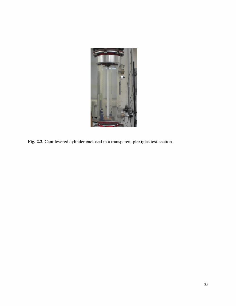
35
Fig. 2.2. Cantilevered cylinder enclosed in a transparent plexiglas test-section.
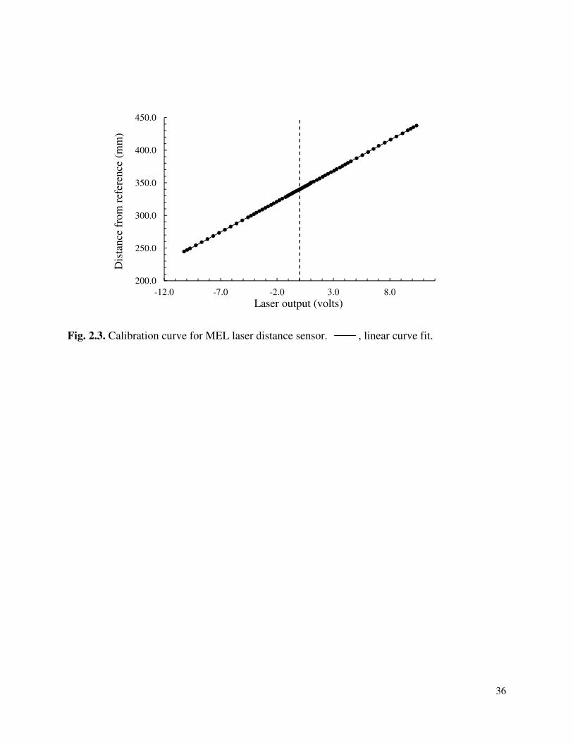
36
Fig. 2.3. Calibration curve for MEL laser distance sensor. , linear curve fit.
200.0
250.0
300.0
350.0
400.0
450.0
-12.0 -7.0 -2.0 3.0 8.0
Dis
tance
fro
m r
efer
ence
(m
m)
Laser output (volts)
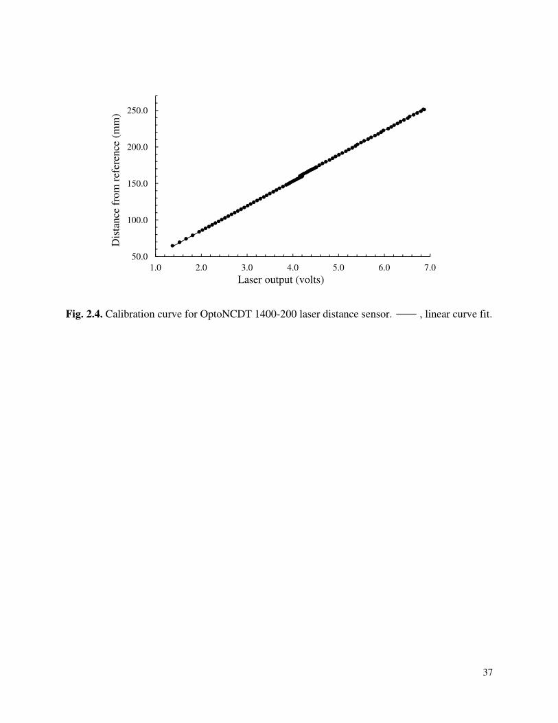
37
Fig. 2.4. Calibration curve for OptoNCDT 1400-200 laser distance sensor. , linear curve fit.
50.0
100.0
150.0
200.0
250.0
1.0 2.0 3.0 4.0 5.0 6.0 7.0
Dis
tance
fro
m r
efer
ence
(m
m)
Laser output (volts)
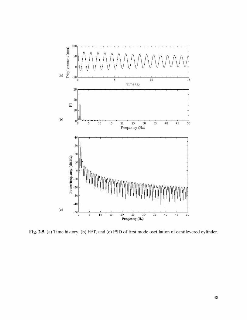
38
Fig. 2.5. (a) Time history, (b) FFT, and (c) PSD of first mode oscillation of cantilevered cylinder.
(a)
(b)
(c)
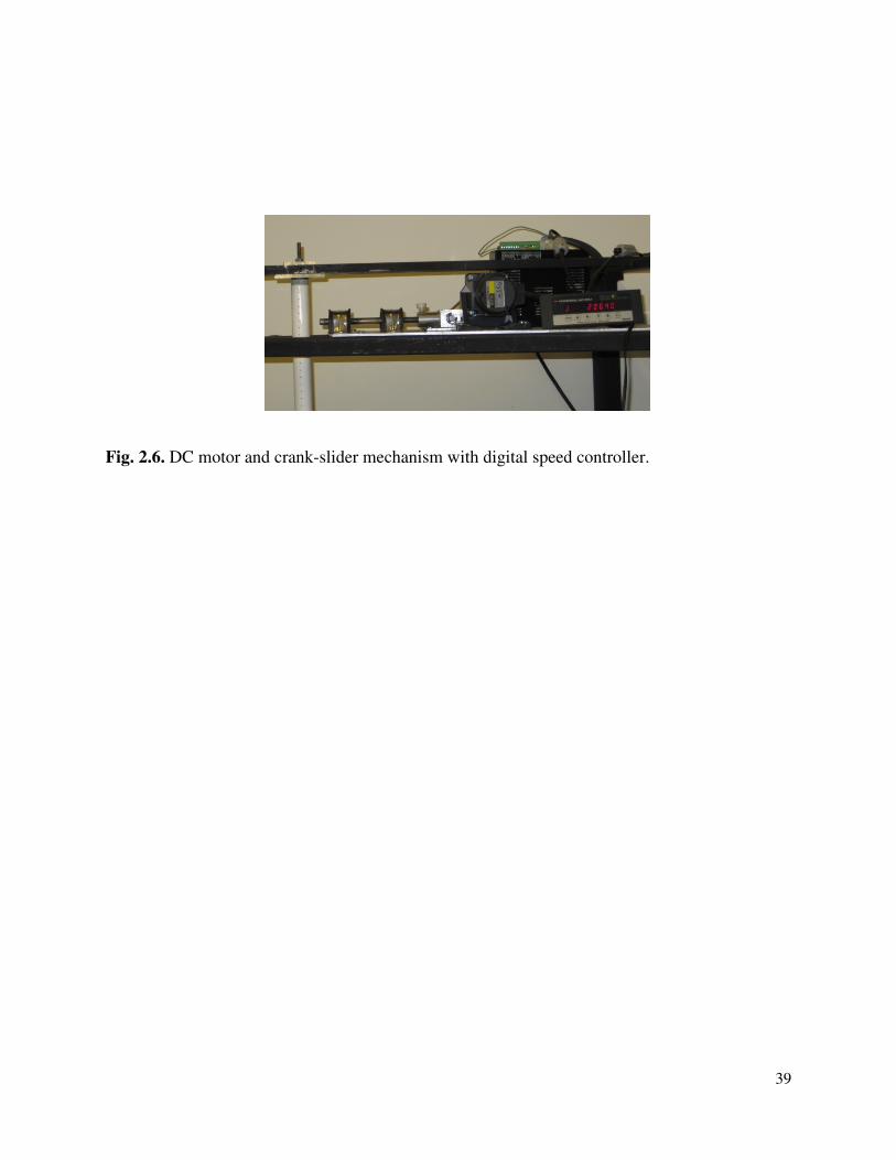
39
Fig. 2.6. DC motor and crank-slider mechanism with digital speed controller.
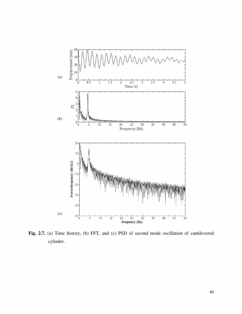
40
Fig. 2.7. (a) Time history, (b) FFT, and (c) PSD of second mode oscillation of cantilevered
cylinder.
(a)
(b)
(c)
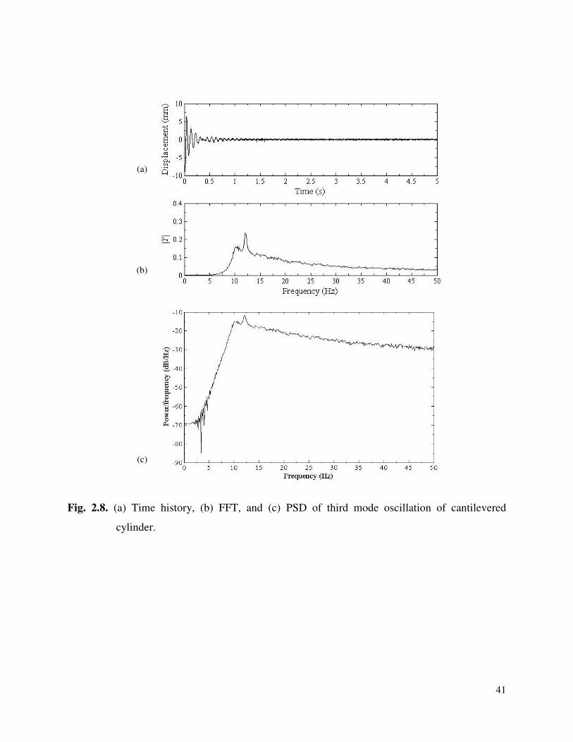
41
Fig. 2.8. (a) Time history, (b) FFT, and (c) PSD of third mode oscillation of cantilevered
cylinder.
(c)
(a)
(b)
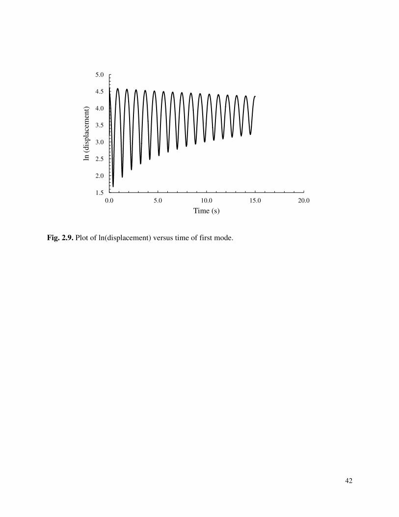
42
Fig. 2.9. Plot of ln(displacement) versus time of first mode.
1.5
2.0
2.5
3.0
3.5
4.0
4.5
5.0
0.0 5.0 10.0 15.0 20.0
ln (
dis
pla
cem
ent)
Time (s)
43
Fig. 2.10. Pitot-static tube and mercury manometer set-up for flow velocity calibration.
44
Fig. 2.11. Plot of height of mercury column versus ATR141 readings. , linear curve fit.
0.0
0.5
1.0
1.5
2.0
2.5
3.0
3.5
4.0
4.5
0.0 50.0 100.0 150.0
Hei
ght
of
Hg c
olu
mn (
in)
ATR141 readings
45
Fig. 2.12. Plot of flow velocity versus ATR141 readings. , polynomial curve fit.
0.0
1.0
2.0
3.0
4.0
5.0
6.0
0.0 20.0 40.0 60.0 80.0 100.0 120.0 140.0 160.0
Flo
w v
eloci
ty (
m/s
)
ATR141 reading
46
Fig. 2.13. Plot of flow velocity versus pump rotational speed. , linear curve fit.
0.0
1.0
2.0
3.0
4.0
5.0
6.0
0.0 200.0 400.0 600.0 800.0 1000.0 1200.0 1400.0 1600.0
Flo
w v
eloci
ty (
m/s
)
Pump r.p.m.
47
Fig. 2.14. (a) Histogram with normal velocity distribution; (b) mean velocity probability plot at
radial distance of 0.0452 m.
0.0
5.0
10.0
15.0
20.0
25.0
1.5 1.7 1.9 2.1 2.3
Per
cent
count
(%)
Velocity (m/s)
(a)
(b)
48
Fig. 2.15. (a) Histogram with normal velocity distribution; (b) mean velocity probability plot at
radial distance of 0.0119 m.
0.0
1.0
2.0
3.0
4.0
5.0
6.0
7.0
8.0
1.0 1.5 2.0 2.5 3.0
Per
cent
count
(%)
Velocity (m/s)
(a)
(b)
49
Fig. 2.16. Turbulent velocity profile inside the test-section. , LDA data; , mean flow
velocity; , polynomial curve fit of LDA data.
0.0
0.5
1.0
1.5
2.0
2.5
0.00 0.02 0.04 0.06 0.08
Flo
w v
eloci
ty (
m/s
)
Distance from the channel wall (m)
50
Fig. 2.17. Turbulent velocity profile obtained from the Flowlite system and logarithmic log law.
, LDA data; , logarithmic log law data; , mean flow velocity;
, polynomial curve fit of LDA data; , polynomial curve fit of logarithmic
log law.
0.0
0.5
1.0
1.5
2.0
2.5
0.00 0.02 0.04 0.06 0.08
Flo
w v
eloci
ty (
m/s
)
Distance from the channel wall (m)
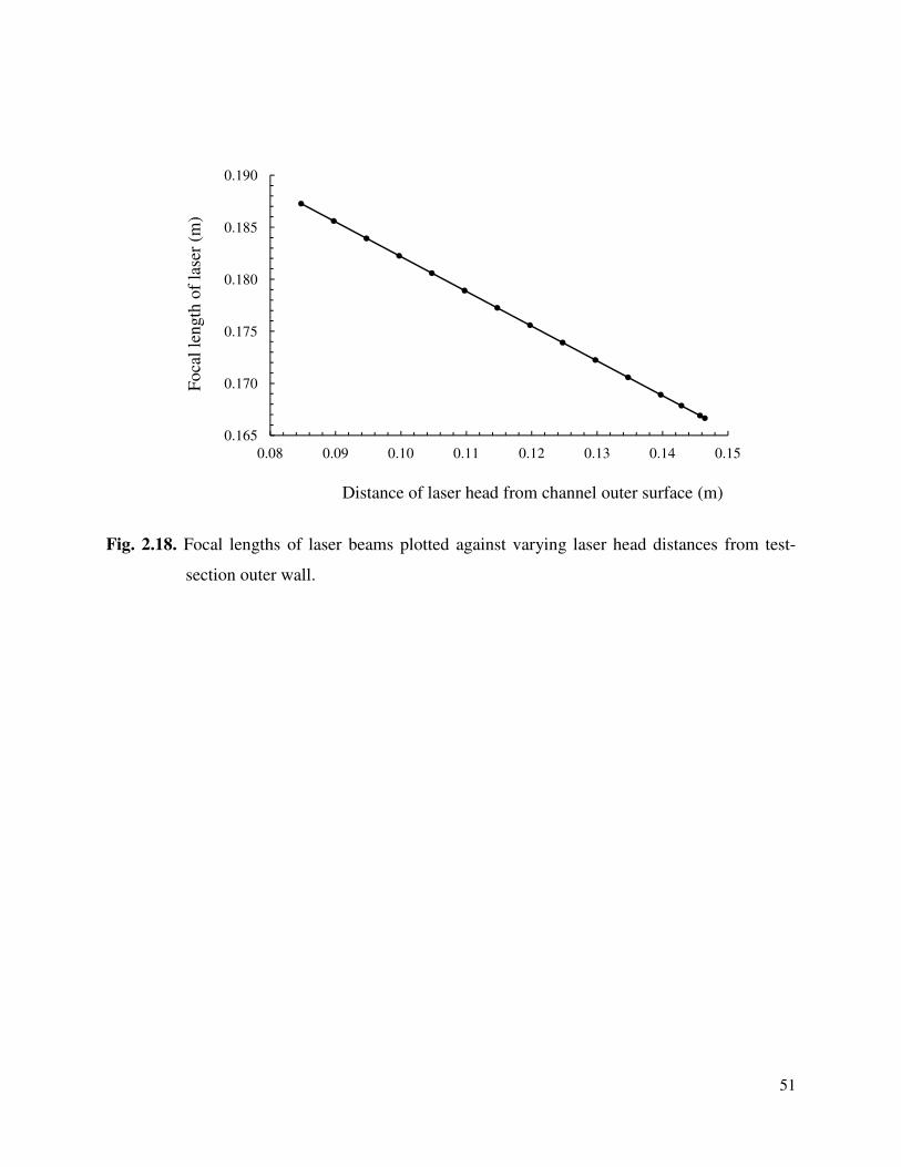
51
Fig. 2.18. Focal lengths of laser beams plotted against varying laser head distances from test-
section outer wall.
0.165
0.170
0.175
0.180
0.185
0.190
0.08 0.09 0.10 0.11 0.12 0.13 0.14 0.15
Foca
l le
ngth
of
lase
r (m
)
Distance of laser head from channel outer surface (m)
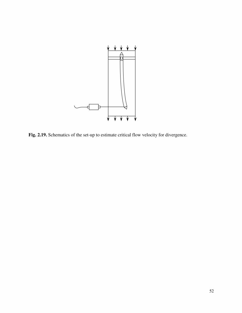
52
Fig. 2.19. Schematics of the set-up to estimate critical flow velocity for divergence.
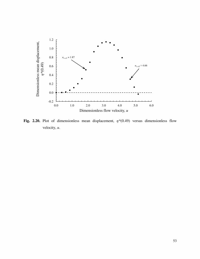
53
Fig. 2.20. Plot of dimensionless mean displacement, η*(0.49) versus dimensionless flow
velocity, u.
-0.2
0.0
0.2
0.4
0.6
0.8
1.0
1.2
0.0 1.0 2.0 3.0 4.0 5.0 6.0
Dim
ensi
onle
ss m
ean d
ispla
cem
ent,
η*(0
.49)
Dimensionless flow velocity, u
ucr,d1 = 1.87
ucr,d2 ≈ 4.66
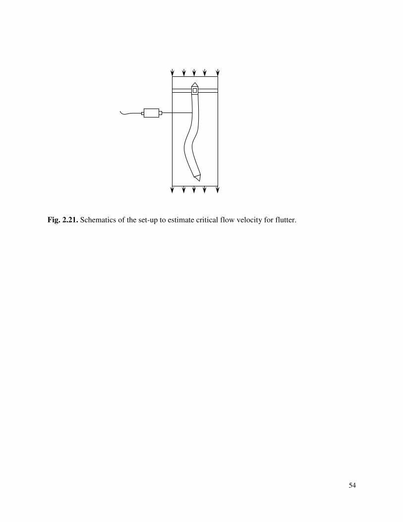
54
Fig. 2.21. Schematics of the set-up to estimate critical flow velocity for flutter.
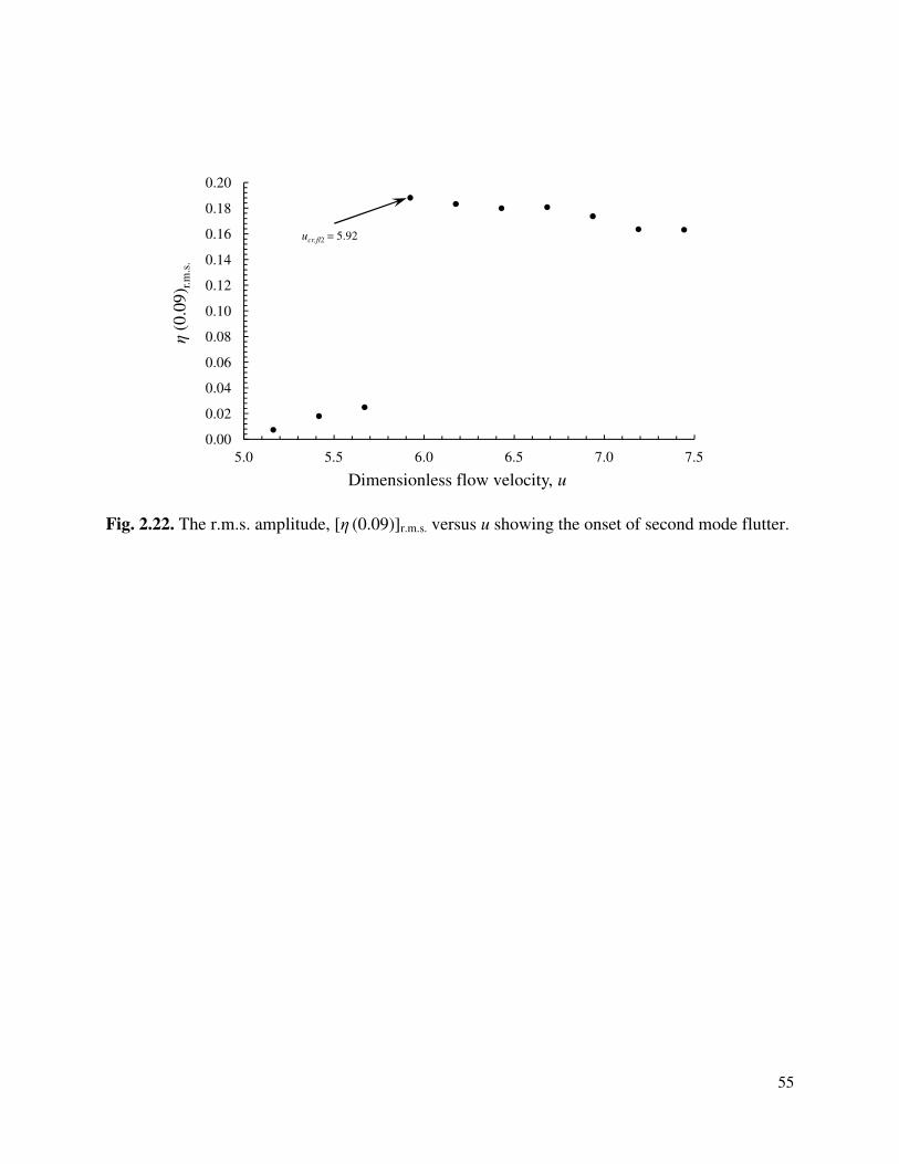
55
Fig. 2.22. The r.m.s. amplitude, [η (0.09)]r.m.s. versus u showing the onset of second mode flutter.
0.00
0.02
0.04
0.06
0.08
0.10
0.12
0.14
0.16
0.18
0.20
5.0 5.5 6.0 6.5 7.0 7.5
η(0
.09) r
.m.s
.
Dimensionless flow velocity, u
ucr,fl2 = 5.92
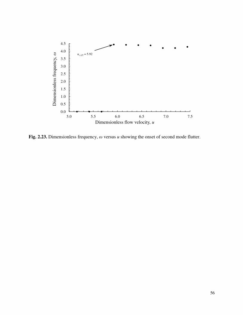
56
Fig. 2.23. Dimensionless frequency, ω versus u showing the onset of second mode flutter.
0.0
0.5
1.0
1.5
2.0
2.5
3.0
3.5
4.0
4.5
5.0 5.5 6.0 6.5 7.0 7.5
Dim
ensi
onle
ss f
requen
cy, ω
Dimensionless flow velocity, u
ucr,fl2 = 5.92
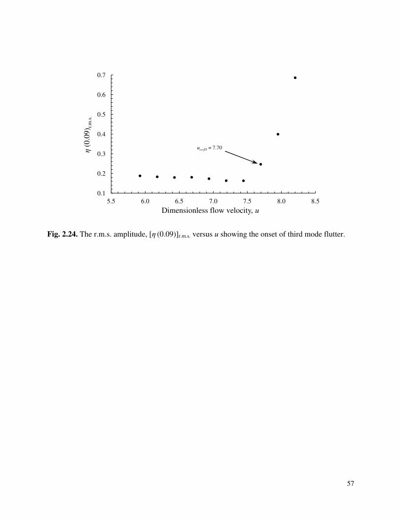
57
Fig. 2.24. The r.m.s. amplitude, [η (0.09)]r.m.s. versus u showing the onset of third mode flutter.
0.1
0.2
0.3
0.4
0.5
0.6
0.7
5.5 6.0 6.5 7.0 7.5 8.0 8.5
η(0
.09) r
.m.s
.
Dimensionless flow velocity, u
ucr,fl3 = 7.70
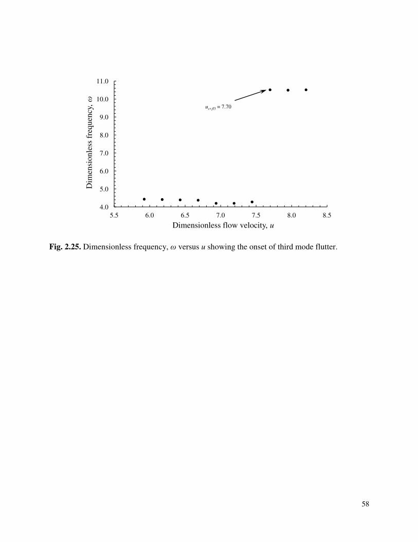
58
Fig. 2.25. Dimensionless frequency, ω versus u showing the onset of third mode flutter.
4.0
5.0
6.0
7.0
8.0
9.0
10.0
11.0
5.5 6.0 6.5 7.0 7.5 8.0 8.5
Dim
ensi
onle
ss f
requen
cy, ω
Dimensionless flow velocity, u
ucr,fl3 = 7.70
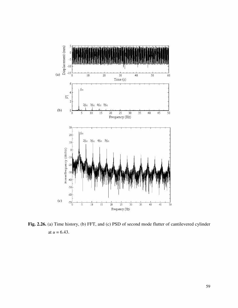
59
Fig. 2.26. (a) Time history, (b) FFT, and (c) PSD of second mode flutter of cantilevered cylinder
at u = 6.43.
(a)
(b)
(c)
ffl2
2ffl2 3ffl2 4ffl2 5ffl2
ffl2
2ffl2 3ffl2 4ffl2 5ffl2
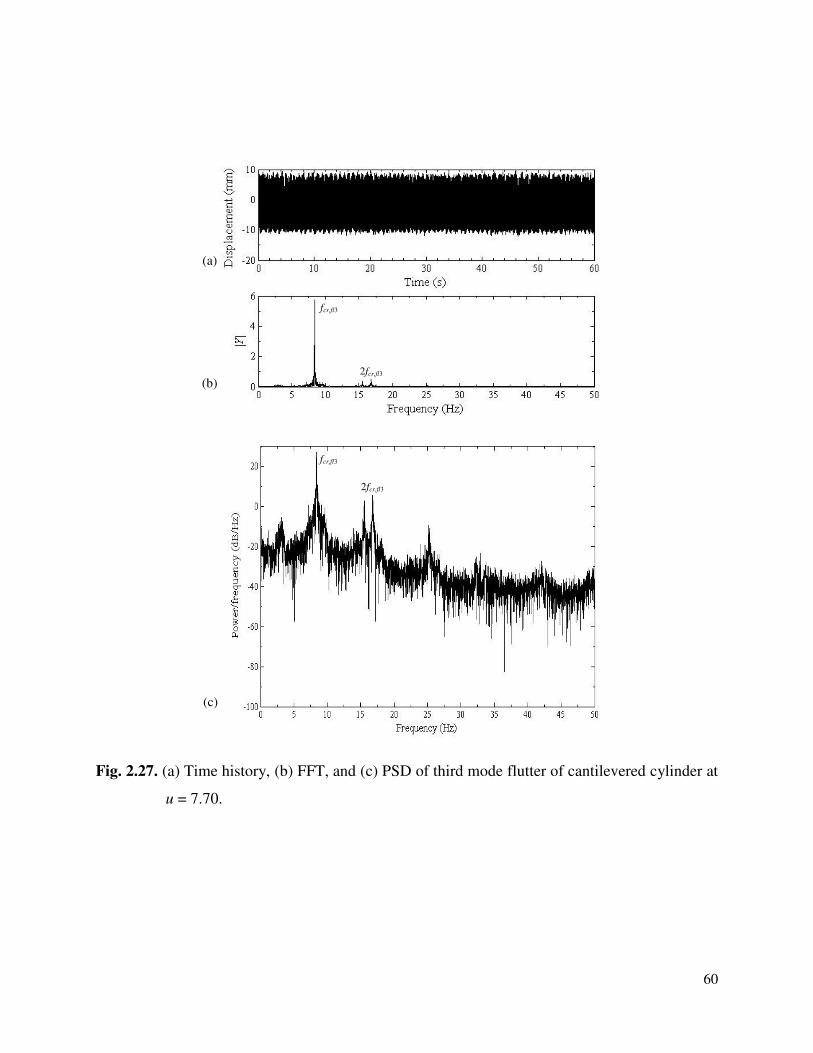
60
Fig. 2.27. (a) Time history, (b) FFT, and (c) PSD of third mode flutter of cantilevered cylinder at
u = 7.70.
(a)
(b)
(c)
fcr,fl3
2fcr,fl3
fcr,fl3
2fcr,fl3
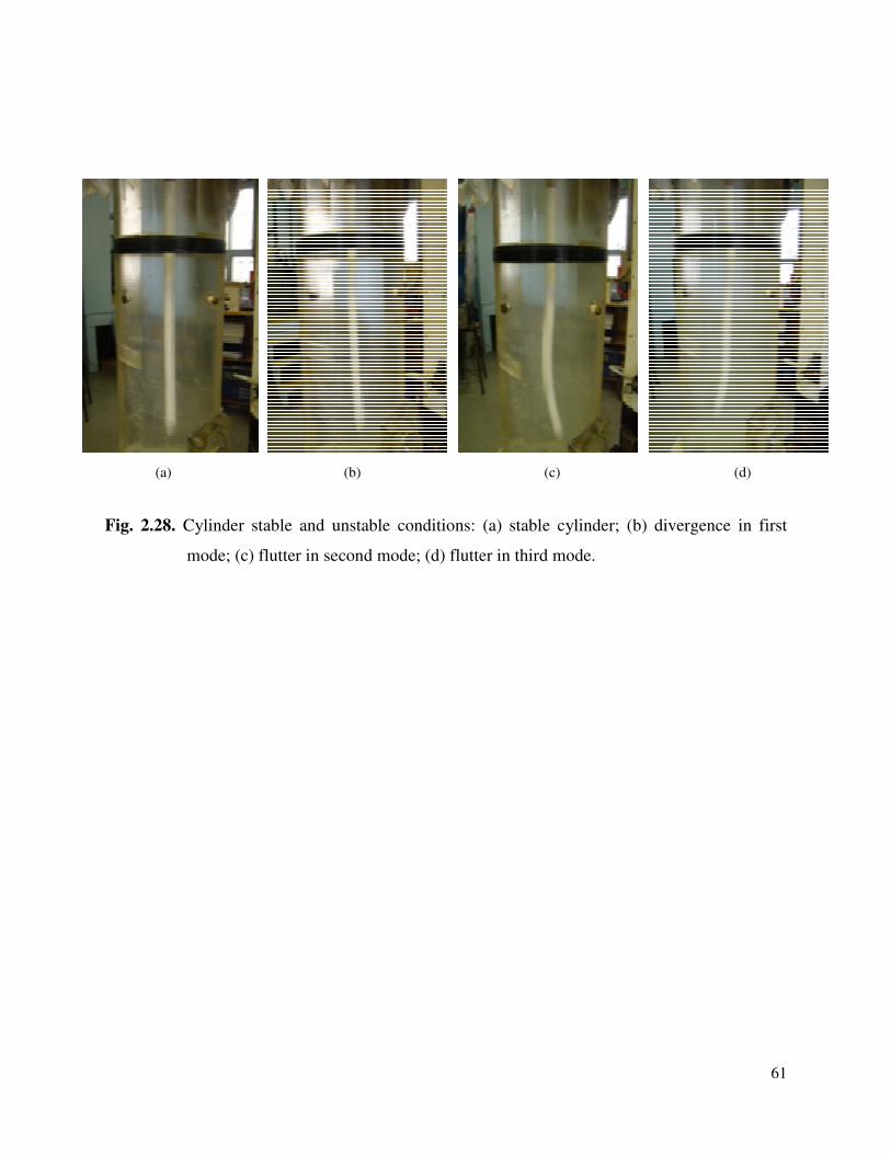
Fig. 2.28. Cylinder stable and unstable conditions: (a) stable cylinder; (b) divergence in first
mode; (c) flutter in second mode; (d) flutter in third mode.
(a)
Cylinder stable and unstable conditions: (a) stable cylinder; (b) divergence in first
mode; (c) flutter in second mode; (d) flutter in third mode.
(b) (c)
61
Cylinder stable and unstable conditions: (a) stable cylinder; (b) divergence in first
(d)
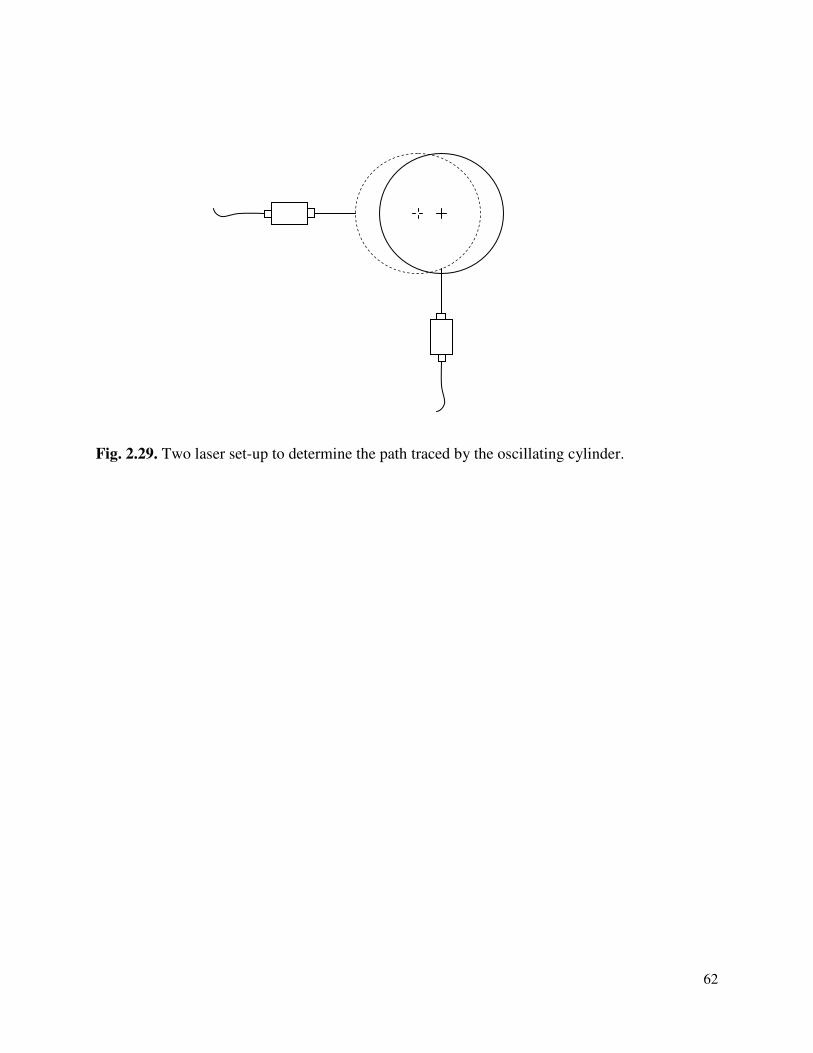
62
Fig. 2.29. Two laser set-up to determine the path traced by the oscillating cylinder.
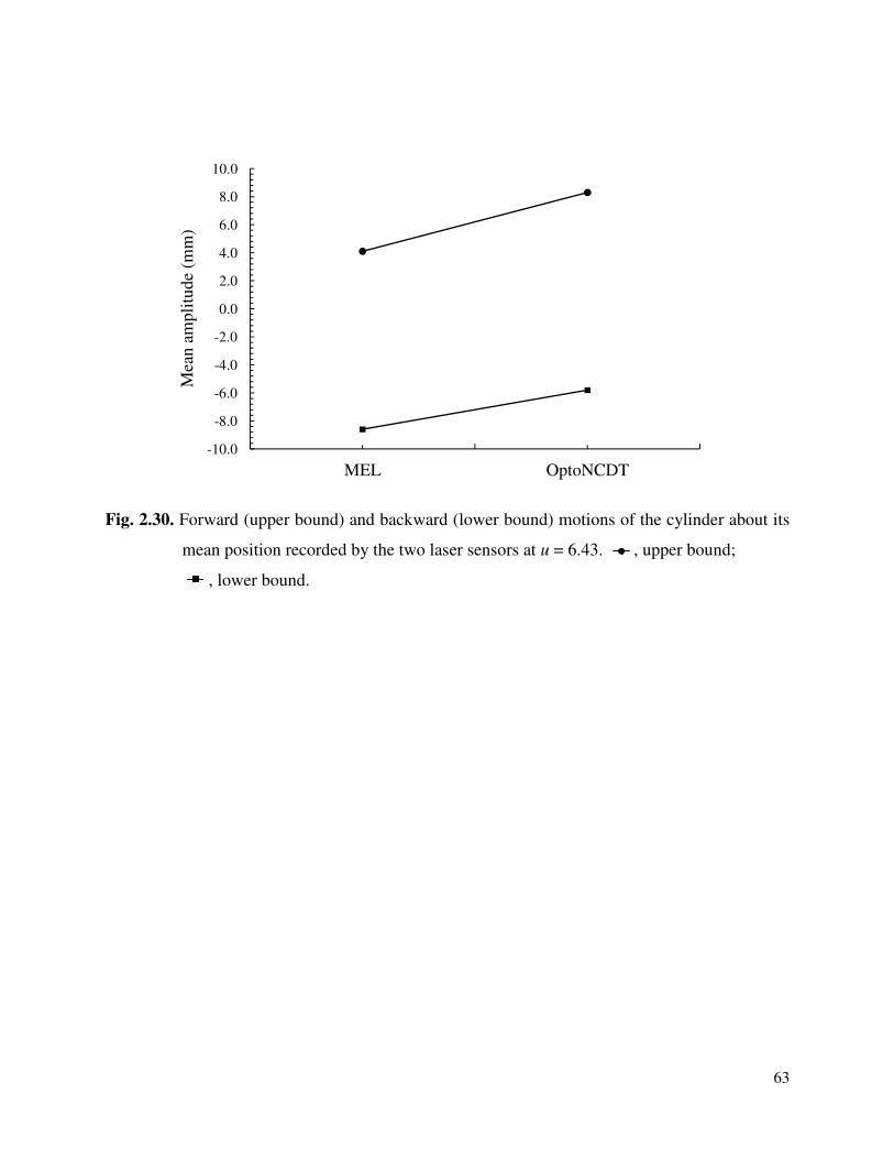
63
Fig. 2.30. Forward (upper bound) and backward (lower bound) motions of the cylinder about its
mean position recorded by the two laser sensors at u = 6.43. , upper bound;
, lower bound.
-10.0
-8.0
-6.0
-4.0
-2.0
0.0
2.0
4.0
6.0
8.0
10.0
MEL OptoNCDT
Mea
n a
mpli
tude
(mm
)
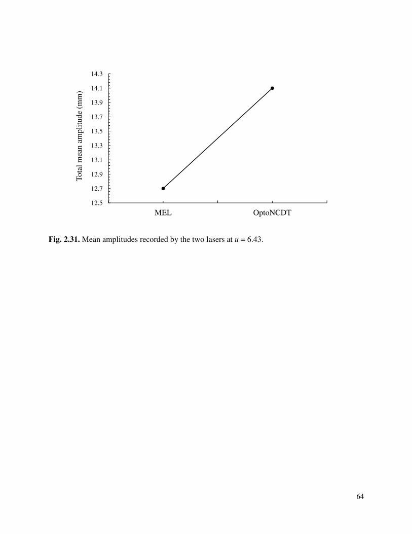
64
Fig. 2.31. Mean amplitudes recorded by the two lasers at u = 6.43.
12.5
12.7
12.9
13.1
13.3
13.5
13.7
13.9
14.1
14.3
MEL OptoNCDT
Tota
l m
ean a
mpli
tude
(mm
)
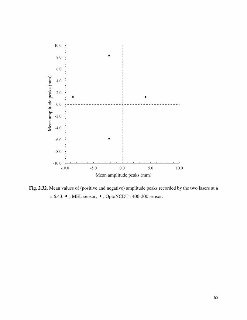
65
Fig. 2.32. Mean values of (positive and negative) amplitude peaks recorded by the two lasers at u
= 6.43. , MEL sensor; , OptoNCDT 1400-200 sensor.
-10.0
-8.0
-6.0
-4.0
-2.0
0.0
2.0
4.0
6.0
8.0
10.0
-10.0 -5.0 0.0 5.0 10.0
Mea
n a
mpli
tude
pea
ks
(mm
)
Mean amplitude peaks (mm)
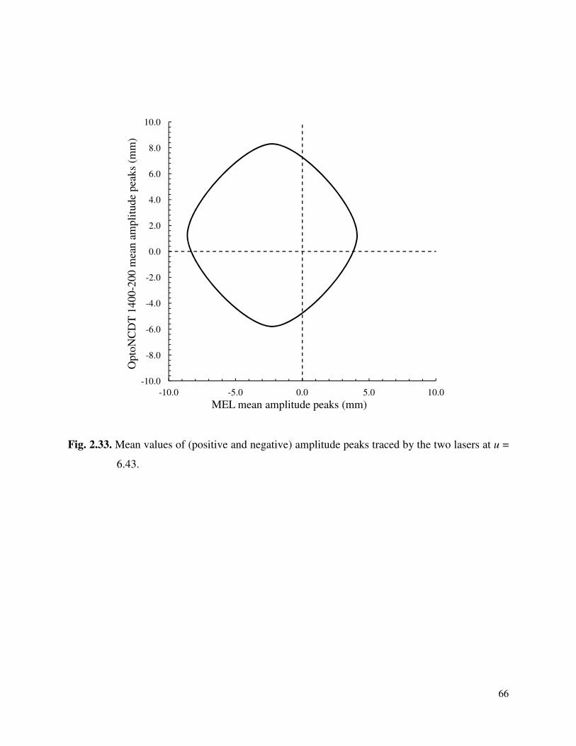
66
Fig. 2.33. Mean values of (positive and negative) amplitude peaks traced by the two lasers at u =
6.43.
-10.0
-8.0
-6.0
-4.0
-2.0
0.0
2.0
4.0
6.0
8.0
10.0
-10.0 -5.0 0.0 5.0 10.0
Opto
NC
DT
1400-2
00 m
ean a
mpli
tude
pea
ks
(mm
)
MEL mean amplitude peaks (mm)
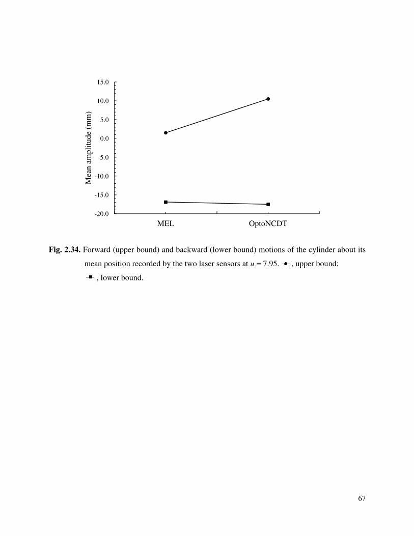
67
Fig. 2.34. Forward (upper bound) and backward (lower bound) motions of the cylinder about its
mean position recorded by the two laser sensors at u = 7.95. , upper bound;
, lower bound.
-20.0
-15.0
-10.0
-5.0
0.0
5.0
10.0
15.0
MEL OptoNCDT
Mea
n a
mpli
tude
(mm
)
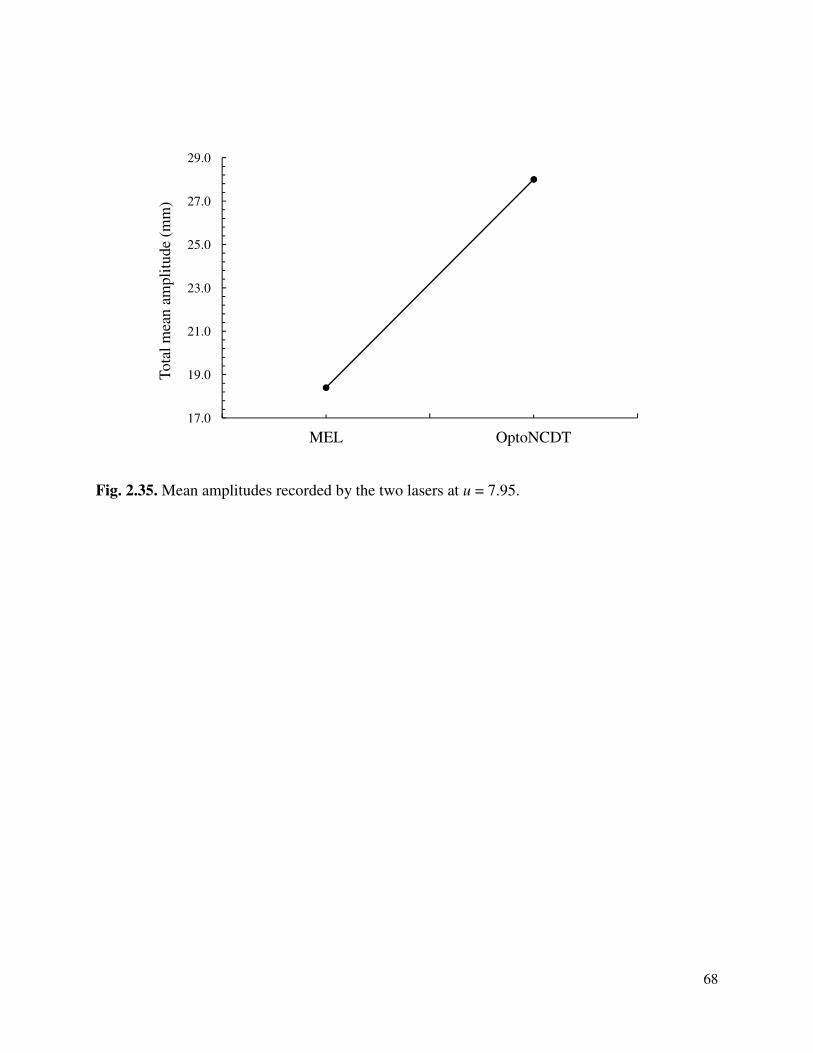
68
Fig. 2.35. Mean amplitudes recorded by the two lasers at u = 7.95.
17.0
19.0
21.0
23.0
25.0
27.0
29.0
MEL OptoNCDT
Tota
l m
ean a
mpli
tude
(mm
)
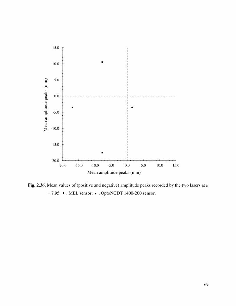
69
Fig. 2.36. Mean values of (positive and negative) amplitude peaks recorded by the two lasers at u
= 7.95. , MEL sensor; , OptoNCDT 1400-200 sensor.
-20.0
-15.0
-10.0
-5.0
0.0
5.0
10.0
15.0
-20.0 -15.0 -10.0 -5.0 0.0 5.0 10.0 15.0
Mea
n a
mpli
tude
pea
ks
(mm
)
Mean amplitude peaks (mm)
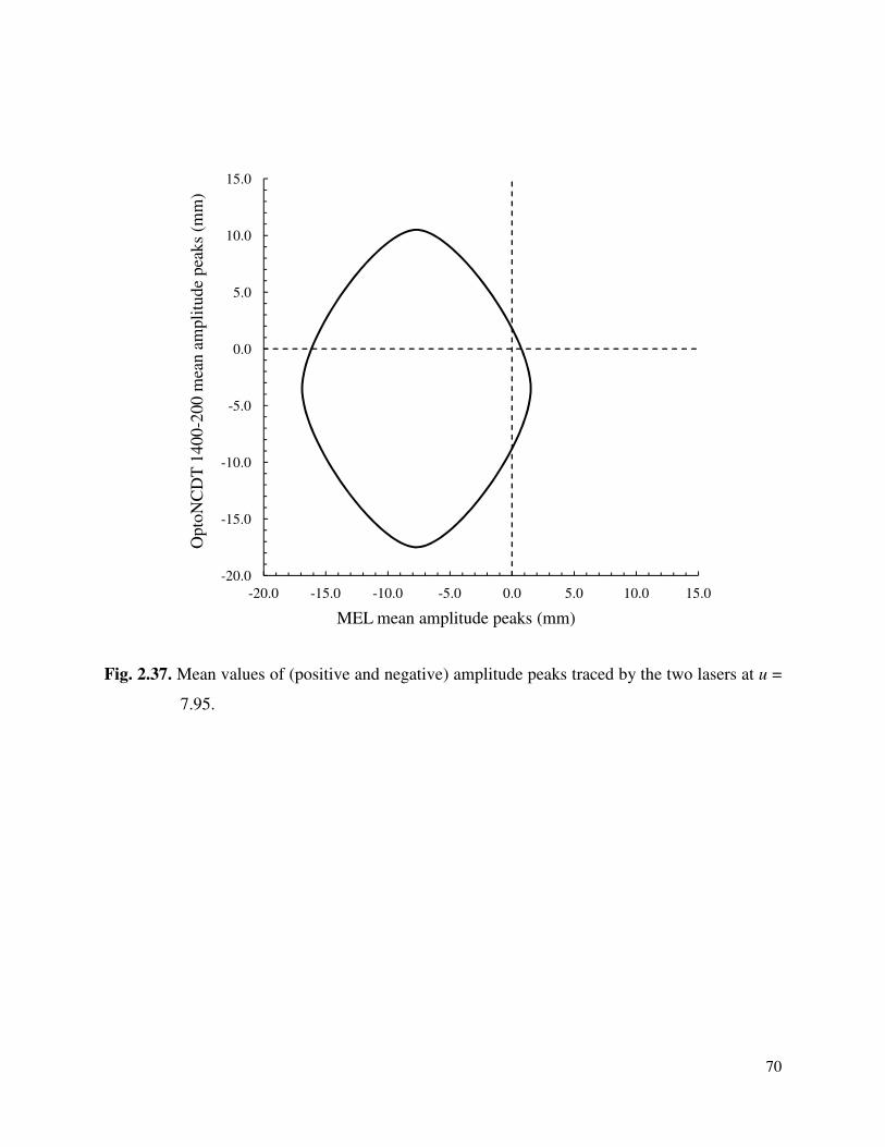
70
Fig. 2.37. Mean values of (positive and negative) amplitude peaks traced by the two lasers at u =
7.95.
-20.0
-15.0
-10.0
-5.0
0.0
5.0
10.0
15.0
-20.0 -15.0 -10.0 -5.0 0.0 5.0 10.0 15.0
Opto
NC
DT
1400-2
00 m
ean a
mpli
tude
pea
ks
(mm
)
MEL mean amplitude peaks (mm)
Chapter 3
Linear Analysis
3.1. Introduction
In the previous theoretical studies on cylindrical system in axial flow with different lengths and
support boundary conditions (Paїdoussis 1966a, 1973; Paїdoussis et al. 1980a; De Langre et al.
2007), the details of which are given in Chapter 1, they formulated the various fluid forces such
as the inviscid forces, viscous forces, and hydrostatic or pressure forces acting on the cylinder.
As a matter of fact, some of the viscous forces are semi-empirical and involve fluid force
coefficients such as longitudinal and normal viscous coefficients, base drag coefficient, and zero-
flow normal force coefficient. In most of the above cited work, they considered equal values for
the longitudinal and normal viscous force coefficients, and considered the base drag coefficient
varying linearly with the end-shape factor f. Hence there is need to re-evaluate these force
coefficients based on the present problem and incorporate in the linear model. It is expected that
the implementation of these calculated coefficients in the linear model will enable the model to
better describe the dynamics of the system.
In addition to obtaining these force coefficients, this chapter also gives an account of the
linear dynamics of a vertical cantilevered flexible cylinder in axial uniform water and air flows.
In this connection, the effect of confinement on the dynamics of the cylindrical system, both in
water and air flows, is also presented. The effect of confinement on the system with the
calculated force coefficients is then presented. The present model results with the previously
reported force coefficients are then compared with those by Paїdoussis (1973) in order to
establish the adequacy of the present solution method. In addition, the present results with
previously used and presently calculated force coefficients are also compared together to see
how these coefficients affect the overall dynamics of the system. Finally, the model results for
water and air flows are compared together to understand the dynamics of the system in different
flow media.
72
3.2. Problem Description
The system under consideration consists of a flexible cylindrical body of radius R, uniform
circular cross-sectional area A, length L, flexural rigidity EI, and mass per unit length m, and
centrally located in a rigid channel of radius Rch as shown in Fig. 3.1 (a). The rigid channel
contains an incompressible fluid of density ρ flowing with uniform flow velocity U parallel to
the axis of the cylinder. The undeformed cylinder axis coincides with the x-axis, and since the
system is vertical, the x-axis is along the same direction of gravitational force. The cylinder is
considered to have cantilevered boundary conditions. The cylinder is generally fitted with an
ogival end-piece at the downstream free end and considered to be short relative to the overall
length of the cylinder as shown in Fig. 3.1 (b). Furthermore, the fluid is assumed to be contained
by boundaries sufficiently distant from the cylinder to have negligible influence on its motion.
The present problem of the dynamics of flexible cylinder in axial flow is a typical FSI problem.
The basic assumptions made for the cylinder and for the fluid are that (a) the fluid is
incompressible, (b) the mean fluid flow velocity is constant, (c) the cylinder is slender, so that
Euler-Bernoulli beam theory remains applicable, (d) although the deflections of the cylinder may
be large, strains are small, and (e) the cylinder centreline is inextensible (Paїdoussis 2004).
3.3. Linear Equation of Motion
Let us consider small lateral motions of the cylinder about its equilibrium position at rest as
shown in Fig. 3.1 (a). Various fluid forces act on the cylinder, the relations of which are
determined as follows: the inviscid hydrodynamic force per unit length, FA, is determined based
on the theory developed by Lighthill (1960); the viscous forces in the normal and longitudinal
direction, FN and FL, respectively, are determined based on Taylor’s work (1952); the hydrostatic
forces in the x- and y- direction, Fpx abd Fpy, respectively, are determined by considering an
element, δx, of the cylinder undergoing small oscillations, y(x, t). The equation of motion of
cylinder, given by Paїdoussis (2004), can be written as
73
( )( )[ ]( )
( )
2
2
22
2
2
4
4*
12
1
2
11
12
1
21
x
y
CUDxL
gAm
D
DCDU
ApT
yx
Ut
Ax
yIE
tE
b
h
T
∂
∂
−+
−
−
−+
+
+−+
−
∂
∂+
∂
∂+
∂
∂
+
∂
∂
δρδ
ρ
ρνδ
χρ
( ) ,02
1
2
1
2
12
22 =
∂
∂+
∂
∂
+−+
∂
∂+
∂
∂+
∂
∂+
t
ym
x
y
D
DCDUgAm
t
yDC
x
yU
t
yDUC
h
NDN ρρρρ (3.1)
where δ = 0 indicates that the downstream end of the cylinder is free to slide axially, and δ = 1 if
the supports do not allow axial extension (Paїdoussis 2004). In eq. (3.1), E is Young’s Modulus,
E* is the corresponding viscoelastic constant, I is the second moment of area, T is externally
imposed uniform tension, ν is Poisson’s ratio, p is the mean value of pressure, p at x = ½ L, CT
and CN are the tangential and normal friction coefficients, respectively, Cb is the base drag
coefficient, CD is form drag coefficient, and m is the mass of the cylinder per unit length. E* is
complex. The real part relates to the elastic behavior of the material and defines stiffness. The
imaginary component relates to the material’s viscous behaviour and defines the energy
dissipation ability of the material. Mathematically, it can be defined as
( ) φεσ ioo eiEEE =+= 21
*. The complete derivation of the linear equation of motion for a
cylinder in axial flow may be found in Paїdoussis (2004).
3.3.1. Boundary Conditions
A set of generalized boundary conditions for cylinders with supported ends is given by
Paїdoussis (2004) as
0 ,03
3
==+∂
∂xatyk
x
yEI o (3.2a)
0 ,02
2
==∂
∂−
∂
∂xat
x
yc
x
yEI o (3.2b)
Lxatykx
yEI L ==−
∂
∂ ,0
3
3
(3.3a)
Lxatx
yc
x
yEI L ==
∂
∂+
∂
∂ ,0
2
2
(3.3b)
74
where, ko and kL are translational spring constants and co and cL rotational ones, for x = 0 and x =
L, respectively. From the above relations, the standard boundary conditions can be extracted
accordingly as ko, kL, co, cL are either zero or infinity.
In the case of a free downstream end, a more general boundary condition is considered to
tackle cases of an ogival free end. The final form obtained is:
0=∂
∂=
x
yy , at x = 0 (3.4)
0)(2
2
3
3
2
2
=∂
∂+−
∂
∂+
∂
∂+
∂
∂=
∂
∂
t
yxfMm
x
yU
t
yfMU
x
yEI
x
ye at x = L , (3.5)
where
( ) AMdxxAA
x
L
lL
e χρ== ∫−
,1
; (3.6)
f is the end-shape factor, which determines the slenderness of the end shape. Its value approaches
1 for an ideally slender end and 0 for a perfectly blunt end. M is the added (virtual) mass of the
fluid per unit length and m is the mass of the cylinder per unit length. χ is defined in Chapter 2. A
complete derivation of this boundary condition is given by Paїdoussis (2004).
3.4. Dimensionless Parameters
In order to render the linear partial differential equation (3.1) and the ogival end-piece boundary
conditions (eq. (3.5)) dimensionless, the following relations are used:
( )( )
EI
gLAm
mA
A
L
E
mAE
I
Am
EI
L
t
L
y
L
x 3
2
*21
21
2 , , , , ,
ργ
ρ
ρβ
ρα
ρτηξ
−=
+=
+=
+===
TTNNff
h
CcCcCcD
Dh
EI
ALpUL
EI
Au
D
L
EI
LT
πππ
ρε
4 ,
4 ,
4 , , , , ,
221
2
=====Π
===Γ
L
xLC
EI
AcCc e
eDbb =
== χ
ρ
ππ ,
4 ,
4 21
. (3.7)
The equation of motion and the boundary conditions for a cantilevered cylinder are thus
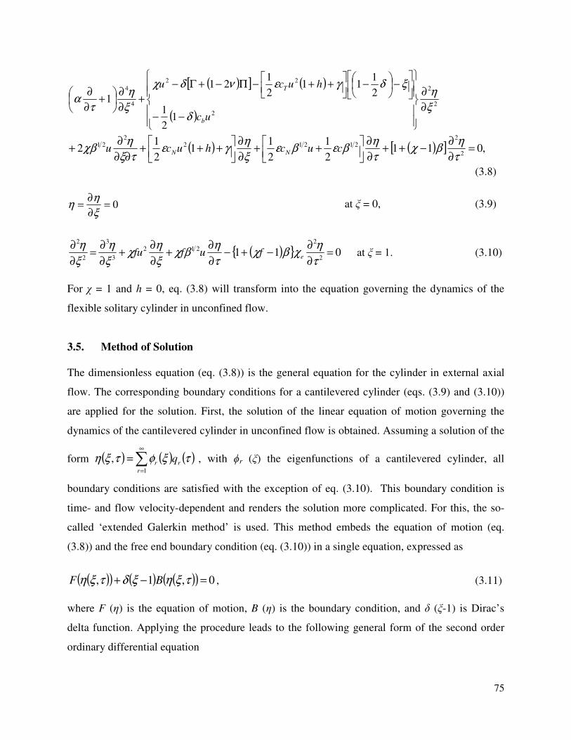
75
( )[ ] ( )
( )2
2
2
22
4
4
12
1
2
111
2
121
1ξ
η
δ
ξδγενδχ
ξ
η
τα
∂
∂
−−
−
−
++−Π−+Γ−
+∂
∂
+
∂
∂
uc
hucu
b
T
( ) ( )[ ] ,0112
1
2
11
2
12
2
221212
221 =
∂
∂−++
∂
∂
++
∂
∂
+++
∂∂
∂+
τ
ηβχ
τ
ηβεβε
ξ
ηγε
τξ
ηχβ cuchucu NN
(3.8)
0=∂
∂=
ξ
ηη at ξ = 0, (3.9)
( ) 0112
2212
3
3
2
2
=∂
∂−+−
∂
∂+
∂
∂+
∂
∂=
∂
∂
τ
ηχβχ
τ
ηβχ
ξ
ηχ
ξ
η
ξ
ηefuffu at ξ = 1. (3.10)
For χ = 1 and h = 0, eq. (3.8) will transform into the equation governing the dynamics of the
flexible solitary cylinder in unconfined flow.
3.5. Method of Solution
The dimensionless equation (eq. (3.8)) is the general equation for the cylinder in external axial
flow. The corresponding boundary conditions for a cantilevered cylinder (eqs. (3.9) and (3.10))
are applied for the solution. First, the solution of the linear equation of motion governing the
dynamics of the cantilevered cylinder in unconfined flow is obtained. Assuming a solution of the
form ( ) ( ) ( )∑∞
=
=1
,r
rr q τξφτξη , with ϕr (ξ) the eigenfunctions of a cantilevered cylinder, all
boundary conditions are satisfied with the exception of eq. (3.10). This boundary condition is
time- and flow velocity-dependent and renders the solution more complicated. For this, the so-
called ‘extended Galerkin method’ is used. This method embeds the equation of motion (eq.
(3.8)) and the free end boundary condition (eq. (3.10)) in a single equation, expressed as
( )( ) ( ) ( )( ) 0,1, =−+ τξηξδτξη BF , (3.11)
where F (η) is the equation of motion, B (η) is the boundary condition, and δ (ξ-1) is Dirac’s
delta function. Applying the procedure leads to the following general form of the second order
ordinary differential equation
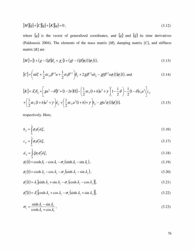
76
[ ] [ ] [ ] 0=++ qKqCqM &&& , (3.12)
where q is the vector of generalized coordinates, and q& and q&& its time derivatives
(Paїdoussis 2004). The elements of the mass matrix [M], damping matrix [C], and stiffness
matrix [K] are
[ ] ( )[ ] ( ) ( ) ( )111111 jrerj fM φφβχχδβχ −++−+= , (3.13)
[ ] ( ) ( )1122
1
2
1 212121214
jrrjrjNr ufubcucC φφβχχβδβεβεαλ −+
++= , and (3.14)
[ ] ( ) ( ) ( ) rjbTrjr cucuhcuK
−−
−
++−Π−+Γ−+= 2224 1
2
1
2
111
2
121 δδγενδχδλ
( ) ( ) ( ) ( ),1112
11
2
1 222
jrrjNrjT fubhucduhc φφχγεγε ′−
+++
+++ (3.15)
respectively. Here,
,
1
0
∫ ′= ξφφ db jrrj (3.16)
,
1
0
∫ ′′= ξφφ dc jrrj (3.17)
,
1
0
∫ ′′= ξφξφ dd jrrj (3.18)
( ) ( )rrrrrr λλσλλφ sinsinhcoscosh1 −−−= , (3.19)
( ) ( )jjjjjj λλσλλφ sinsinhcoscosh1 −−−= , (3.20)
( ) ( )[ ]jjrjjjj λλσλλλφ coscoshsinsinh1 −−+=′ , (3.21)
( ) ( )[ ]jjrjjjj λλσλλλφ sinsinhcoscosh1
2 +−+=′′ , (3.22)
rr
rrr
λλ
λλσ
coscosh
sinsinh
+
−= , (3.23)
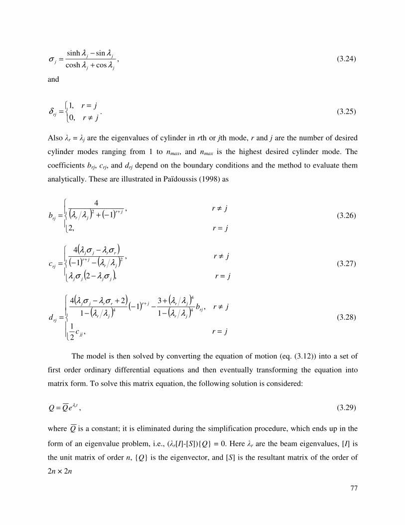
77
jj
jj
jλλ
λλσ
coscosh
sinsinh
+
−= , (3.24)
and
≠
==
jr
jrrj
,0
,1δ . (3.25)
Also λr = λj are the eigenvalues of cylinder in rth or jth mode, r and j are the number of desired
cylinder modes ranging from 1 to nmax, and nmax is the highest desired cylinder mode. The
coefficients brj, crj, and drj depend on the boundary conditions and the method to evaluate them
analytically. These are illustrated in Paїdoussis (1998) as
( ) ( )
=
≠−+=
+
jr
jrb
jr
jrrj
,2
,1
42
λλ (3.26)
( )( ) ( )
( )
=−
≠−−
−
=+
jr
jrc
jjjj
jr
jr
rrjj
rj
,2
,1
42
σλσλ
λλ
σλσλ
(3.27)
( )( )
( )( )( )
=
≠−
+−−
−
+−
=
+
jrc
jrb
d
jj
rj
jr
jrjr
jr
rrjj
rj
,2
1
,1
31
1
244
4
4λλ
λλ
λλ
σλσλ
(3.28)
The model is then solved by converting the equation of motion (eq. (3.12)) into a set of
first order ordinary differential equations and then eventually transforming the equation into
matrix form. To solve this matrix equation, the following solution is considered:
treQQ
λ= , (3.29)
where Q is a constant; it is eliminated during the simplification procedure, which ends up in the
form of an eigenvalue problem, i.e., (λr[I]-[S])Q = 0. Here λr are the beam eigenvalues, [I] is
the unit matrix of order n, Q is the eigenvector, and [S] is the resultant matrix of the order of
2n × 2n
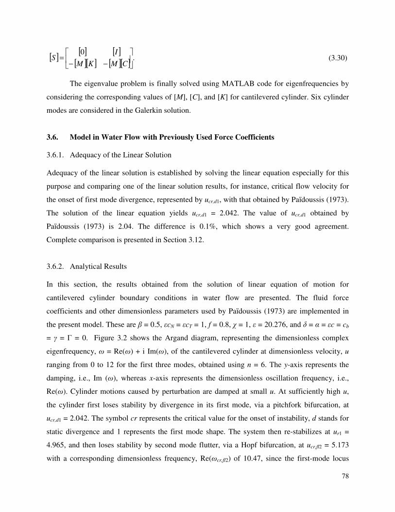
78
[ ][ ] [ ]
[ ][ ] [ ][ ].
0
−−=
CMKM
IS (3.30)
The eigenvalue problem is finally solved using MATLAB code for eigenfrequencies by
considering the corresponding values of [M], [C], and [K] for cantilevered cylinder. Six cylinder
modes are considered in the Galerkin solution.
3.6. Model in Water Flow with Previously Used Force Coefficients
3.6.1. Adequacy of the Linear Solution
Adequacy of the linear solution is established by solving the linear equation especially for this
purpose and comparing one of the linear solution results, for instance, critical flow velocity for
the onset of first mode divergence, represented by ucr,d1, with that obtained by Paїdoussis (1973).
The solution of the linear equation yields ucr,d1 = 2.042. The value of ucr,d1 obtained by
Paїdoussis (1973) is 2.04. The difference is 0.1%, which shows a very good agreement.
Complete comparison is presented in Section 3.12.
3.6.2. Analytical Results
In this section, the results obtained from the solution of linear equation of motion for
cantilevered cylinder boundary conditions in water flow are presented. The fluid force
coefficients and other dimensionless parameters used by Paїdoussis (1973) are implemented in
the present model. These are β = 0.5, εcN = εcT = 1, f = 0.8, χ = 1, ε = 20.276, and δ = α = εc = cb
= γ = Γ = 0. Figure 3.2 shows the Argand diagram, representing the dimensionless complex
eigenfrequency, ω = Re(ω) + i Im(ω), of the cantilevered cylinder at dimensionless velocity, u
ranging from 0 to 12 for the first three modes, obtained using n = 6. The y-axis represents the
damping, i.e., Im (ω), whereas x-axis represents the dimensionless oscillation frequency, i.e.,
Re(ω). Cylinder motions caused by perturbation are damped at small u. At sufficiently high u,
the cylinder first loses stability by divergence in its first mode, via a pitchfork bifurcation, at
ucr,d1 = 2.042. The symbol cr represents the critical value for the onset of instability, d stands for
static divergence and 1 represents the first mode shape. The system then re-stabilizes at ur1 =
4.965, and then loses stability by second mode flutter, via a Hopf bifurcation, at ucr,fl2 = 5.173
with a corresponding dimensionless frequency, Re(ωcr,fl2) of 10.47, since the first-mode locus
79
enters the unstable region at this critical flow velocity while Re(ω) (the real part of the complex
eigenfrequency) remains positive. It then re-stabilizes at ur2 = 8.677, but, before that, it loses
stability again via Hopf bifurcation at ucr,fl3 = 8.311 in the third mode by flutter. Re(ωcr,fl3) at this
critical velocity is 32.46. It is worth reiterate that divergence is a static instability with no
frequency whereas flutter is a dynamic instability with finite frequency.
Figures 3.3 and 3.4 show the dimensionless oscillation frequency, i.e., the real part of the
complex eigenfrequency, and damping, i.e., the imaginary part of the complex eigenfrequency,
respectively, for the first three cylinder modes as function of the dimensionless flow velocity u
for a cantilevered cylinder. For the values of u in the range 0 ≤ u ≤ ucr,d1, the real part of
eigenfrequency continues to decrease until, at a certain flow velocity, the eigenfrequency
becomes purely imaginary, i.e., Re(ω) becomes zero. As u continues to increase, Im(ω) becomes
negative and this is the critical value of u, i.e., ucr,d1 at which the system loses its stability by
divergence in its first mode. At an even higher velocity, i.e., ucr,d1 ≤ u ≤ ucr,fl3, the system
undergoes second and third mode flutter with non-zero values of Re(ωcr,fl), as shown in Figs. 3.3
and 3.4.
3.7. Model in Air Flow
3.7.1. Analytical Results
In this section, the results obtained from the solution of linear equation of motion for a
cantilevered cylinder in air flow are presented. The generation and inclusion of the model
subjected to axial air flow in this chapter is motivated as a limiting case by the motion of a long
train with the last carriage having a tapered end inside a tunnel. The motion of the train in
stationary air inside the tunnel produces the same effects of fluid forces on the train as for a
stationary train subjected to axial air flow inside the tunnel. Cantilevered cylinder model is
considered in air flow since this model is also going to be developed and simulated in other
modeling software and then compared with the analytical results presented in this section. In
order to make the code run for air flow, the value of mass ratio, β is the parameter to modify. It is
dimensionless number and is defined as
mA
A
+=
ρ
ρβ , (3.31)
80
as given in Paїdoussis (2004). Its value for air is 1.074×10⁻³
. Other input parameters are kept the
same as for the cantilevered cylinder model in water flow. Figure 3.5 shows the Argand diagram,
representing the dimensionless complex eigenfrequency, ω = Re(ω) + i Im(ω), of the
cantilevered cylinder as a function of the dimensionless velocity, u, ranging from 0 to 12 for the
first three modes in air flow. Cylinder motions are damped at low flow velocities. At sufficiently
high flow velocity, the complex eigenfrequency of the first mode becomes purely imaginary,
bifurcating on the Im (ω)-axis with Re(ω) = 0. At ucr,d1 = 2.042, one of its branches becomes
negative leading to the onset of divergence in first mode via a pitchfork bifurcation. As the flow
velocity increases, the system losses stability in the second mode via a Hopf bifurcation at ucr,fl2
= 3.470 with dimensionless frequency, Re(ωcr,fl2) = 13.57. It is seen in the figure that with
increasing flow velocity, the second mode in the unstable region bifurcates on the Im (ω)-axis at
ucr,d2 = 4.965 marking divergence in the second mode. Later, the cylinder develops divergence in
the third mode at ucr,d3 = 9.541. In the present model, u = 4.965 is marked as the beginning of the
second zone of divergence.
A similar trend of the re-occurrence of divergence at high flow velocities for very small β
was indicated by Semler et al. (2002). They solved the linear equation of motion with
cantilevered boundary conditions for 0 < β < 1. They observed that for β < 0.38, the system never
re-stabilizes after divergence, but goes to second and higher mode flutter. On the basis of their
results, they established a value of u = 9.6 representing the second zone of divergence. The
difference between the flow velocity commencing the second zone of divergence in the present
model (u = 4.965) and the one (u = 9.6) established by Semler et al. (2002) is due to different
values of εcN (0.5), εcT (0.5), and cb (0.3) used by them, as compared to those used in the present
model (εcN = 1, εcN = 1, and cb = 0). Figures 3.6 and 3.7 show the dimensionless oscillation
frequency and damping for the first three cylinder modes as function of the dimensionless flow
velocity u for the cantilevered cylinder in air flow.
3.8. Effect of Confinement
3.8.1. Model in Water Flow
The effect of confinement on the critical value of u for the onset of divergence and flutter of
cylinder in water flow is considered. It is recalled that the confinement factor is
81
−
+=
22
22
DD
DD
ch
chχ . (3.32)
Using eq. (3.32), values of χ are varied from 1.01 to 2.00. These values are obtained by
keeping the cylinder diameter, D, fixed while reducing the channel diameter. Another useful
parameter associated with confinement is α, the ratio of channel to cylinder diameters,
.D
Dch=α (3.33)
Table 3.1 shows the values of α corresponding to those of χ. Higher values of α signify
low confinement and vice versa. The critical values of the flow velocity for the onset of
divergence and flutter vary with confinement, as shown in Figs. 3.8 - 3.10. With increasing
confinement, viscous effects become more pronounced and the streamwise pressure drop
acquires considerable value. This results in the divergence of the cylinder occurring earlier at
lower velocity, as shown in Fig. 3.8. A similar trend is observed in second and third mode flutter
instabilities as shown in Figs 3.9 and 3.10, respectively.
3.8.2. Model in Air Flow
Next, the effect of confinement on the critical value of u for the onset of divergence and flutter of
cylinder in air flow is analyzed. Similar to the case for water flow, values of confinement factor,
χ, are varied from 1.01 to 2.00. The results of the critical values of flow velocity for the onset of
divergence and flutter varying with confinement are shown in Figs. 3.11 and 3.12, respectively.
The general trend in both the figures show the occurrences of first mode divergence and second
mode flutter at decreasing critical flow velocities with increasing confinement. This can be
attributed to viscous effects and the stream-wise pressure drop becoming more pronounced with
increasing confinement.
3.9. Force Coefficients
Equation (3.8) governs the dynamics of the flexible cylindrical system. Force coefficients in the
equation, i.e., the longitudinal viscous coefficient, cT, normal viscous coefficient, cN, base drag
coefficient, cb, and zero-flow normal coefficient, c play vital role in the energy transfer and
hence the system dynamics. Therefore, determining these force coefficients is imperative. These
82
are expected to be more precisely representing the fluid forces affecting the cylindrical system
dynamics. Hence, these force coefficients, once calculated, are going to be used in the linear
model instead of the previously used ones by Paїdoussis (1973). This section provides a step-by-
step procedure to calculate these coefficients for a given fluid and model geometry, and
discusses the factors affecting these coefficients.
3.9.1. Longitudinal Viscous Coefficient, cT
Viscous forces acting on slender inclined cylinders are discussed by Taylor (1952) in relation to
the swimming of long narrow animals such as snakes, eels, and marine worms. He idealized the
motion of these animals in water producing propulsion by considering the equilibrium of slender
flexible cylinders having bending waves traveling down the cylinder at constant amplitude and
speed in water. He formulated specifically the viscous fluid forces in transverse (N) and
longitudinal (L) directions acting on the flexible smooth and rough cylinders inclined at certain
angles to the flow direction. As limiting cases of a rough cylinder, he presented the expressions
of transverse and longitudinal viscous forces for string like cylinders and cylinders with thin
disks or plates set at right angles to the cylinder axis. He symbolized the force coefficients
associated to the form and friction drag by [CD]p and Cf, respectively.
In case of cylinder surface roughness, Taylor noticed that the boundary layer does not
remain laminar and that the viscous forces rely on the nature of surface roughness (Paїdoussis
2004). He proposed the longitudinal viscous force per unit length, FL as
iCDUF fL cos2
1 2ρ= , (3.34)
where D is the cylinder diameter, Cf is the coefficient associated with friction drag for a cylinder
in cross-flow, defining i as
( ) ( )[ ]Utyxyi ∂∂+∂∂= −− 11 tantan . (3.35)
For small motions, eq. (3.34) may be linearized and, using eq. (3.35), the viscous force
may be represented by
TL CDUF 2
2
1ρ= , (3.36)
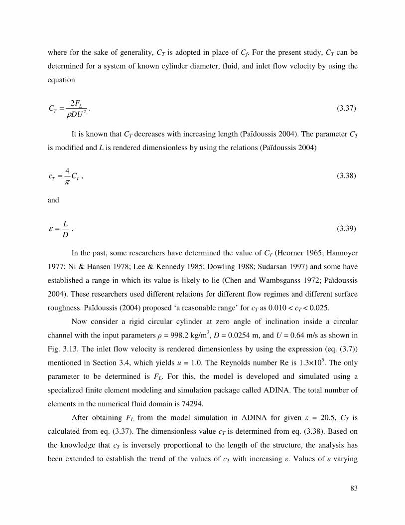
83
where for the sake of generality, CT is adopted in place of Cf. For the present study, CT can be
determined for a system of known cylinder diameter, fluid, and inlet flow velocity by using the
equation
2
2
DU
FC L
Tρ
= . (3.37)
It is known that CT decreases with increasing length (Paїdoussis 2004). The parameter CT
is modified and L is rendered dimensionless by using the relations (Paїdoussis 2004)
TT Ccπ
4= , (3.38)
and
D
L=ε . (3.39)
In the past, some researchers have determined the value of CT (Heorner 1965; Hannoyer
1977; Ni & Hansen 1978; Lee & Kennedy 1985; Dowling 1988; Sudarsan 1997) and some have
established a range in which its value is likely to lie (Chen and Wambsganss 1972; Paїdoussis
2004). These researchers used different relations for different flow regimes and different surface
roughness. Paїdoussis (2004) proposed ‘a reasonable range’ for cT as 0.010 < cT < 0.025.
Now consider a rigid circular cylinder at zero angle of inclination inside a circular
channel with the input parameters ρ = 998.2 kg/m3, D = 0.0254 m, and U = 0.64 m/s as shown in
Fig. 3.13. The inlet flow velocity is rendered dimensionless by using the expression (eq. (3.7))
mentioned in Section 3.4, which yields u = 1.0. The Reynolds number Re is 1.3×10⁵. The only
parameter to be determined is FL. For this, the model is developed and simulated using a
specialized finite element modeling and simulation package called ADINA. The total number of
elements in the numerical fluid domain is 74294.
After obtaining FL from the model simulation in ADINA for given ε = 20.5, CT is
calculated from eq. (3.37). The dimensionless value cT is determined from eq. (3.38). Based on
the knowledge that cT is inversely proportional to the length of the structure, the analysis has
been extended to establish the trend of the values of cT with increasing ε. Values of ε varying
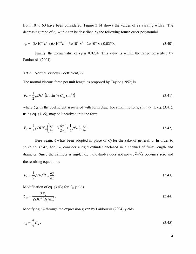
84
from 10 to 60 have been considered. Figure 3.14 shows the values of cT varying with ε. The
decreasing trend of cT with ε can be described by the following fourth order polynomial
0259.0102103106103 4253647 +×−×−×+×−= −−−− εεεεTc . (3.40)
Finally, the mean value of cT is 0.0234. This value is within the range prescribed by
Paїdoussis (2004).
3.9.2. Normal Viscous Coefficient, cN
The normal viscous force per unit length as proposed by Taylor (1952) is
( )iCiCDUF DpfN
22 sinsin2
1+= ρ , (3.41)
where CDp is the coefficient associated with form drag. For small motions, sin i << 1, eq. (3.41),
using eq. (3.35), may be linearized into the form
t
yDC
x
yU
t
yDUCF
DNN∂
∂+
∂
∂+
∂
∂= ρρ
2
1
2
1. (3.42)
Here again, CN has been adopted in place of Cf for the sake of generality. In order to
solve eq. (3.42) for CN, consider a rigid cylinder enclosed in a channel of finite length and
diameter. Since the cylinder is rigid, i.e., the cylinder does not move, ty ∂∂ becomes zero and
the resulting equation is
dx
dyCDUF NN
2
2
1ρ= . (3.43)
Modification of eq. (3.43) for CN yields
( )dxdyDU
FC N
N 2
2
ρ= . (3.44)
Modifying CN through the expression given by Paїdoussis (2004) yields
NN Ccπ
4= . (3.45)
85
Despite the consensus of researchers’ view that cN ≠ cT at least for solitary cylinders,
some have considered cN = cT for their research work (Paїdoussis 1966a 1973; Triantafyllou and
Chryssostomidis 1985). Different values and ranges of cN are found in the literature (Ortloff and
Ives 1969; Chen and Wambsganss 1972; Lee and Kennedy 1985; Dowling 1988). Paїdoussis
(2004) proposed a range of cN well suited to the pertaining research cases, in general as 0.005 <
cN < 0.040.
The known input parameters of the model are ρ = 998.2 kg/m3, D = 0.0254 m, and U =
0.64 m/s. The corresponding dimensionless inlet flow velocity u and Reynolds number Re are
1.0 and 1.3×10⁵, respectively. In order to find the normal viscous force per unit length FN, the
cylinder needs to be inclined at an angle θ to the longitudinal axis of the channel, since FN does
not exist at zero angle of inclination. By doing this, the transverse inviscid hydrodynamic force
or lift force also comes into play and becomes a part of the normal component of the viscous
force; hence its effect should be removed. This is done by subtracting the inviscid force from the
viscous force,
force inviscidforce viscous −=F . (3.46)
The normal component of the resultant force F is the normal viscous force per unit
length, FN = F sin θ. The model is developed and simulated in ADINA to find FN. The total
number of element in the numerical fluid domain is 71279. The cylinder with different angles of
inclination to the fluid flow θ = 5o, 10
o, 15
o, 20
o and slenderness factors, ε = 5, 10, 15, 20, 30, 40,
50 are considered. The ratio dxdy is the slope of the angle of inclination. The model with
inclined cylinder is shown in Fig. 3.15. The mean value of FN for each θ has been substituted
into eq. (3.44) to obtain CN. The final mean value of cN is 0.0041. It is slightly lower than the
minimum suggested value by Paїdoussis (2004), but still within acceptable range as used by
other researchers.
Figure 3.16 shows the variation of FN with ε at different angles of inclination of the
cylinder with respect to channel axis. It is obvious from the figure that, with increasing ε, FN also
increases depicting that normal viscous force per unit length is more pronounced for longer or
wider cylinders. A similar trend is shown in Fig. 3.17, in which FN has been plotted against θ at
different values of ε. Increasing the angle of inclination of the structure enhances the contribution
of the normal viscous force component per unit length, i.e., FN in the overall viscous force.
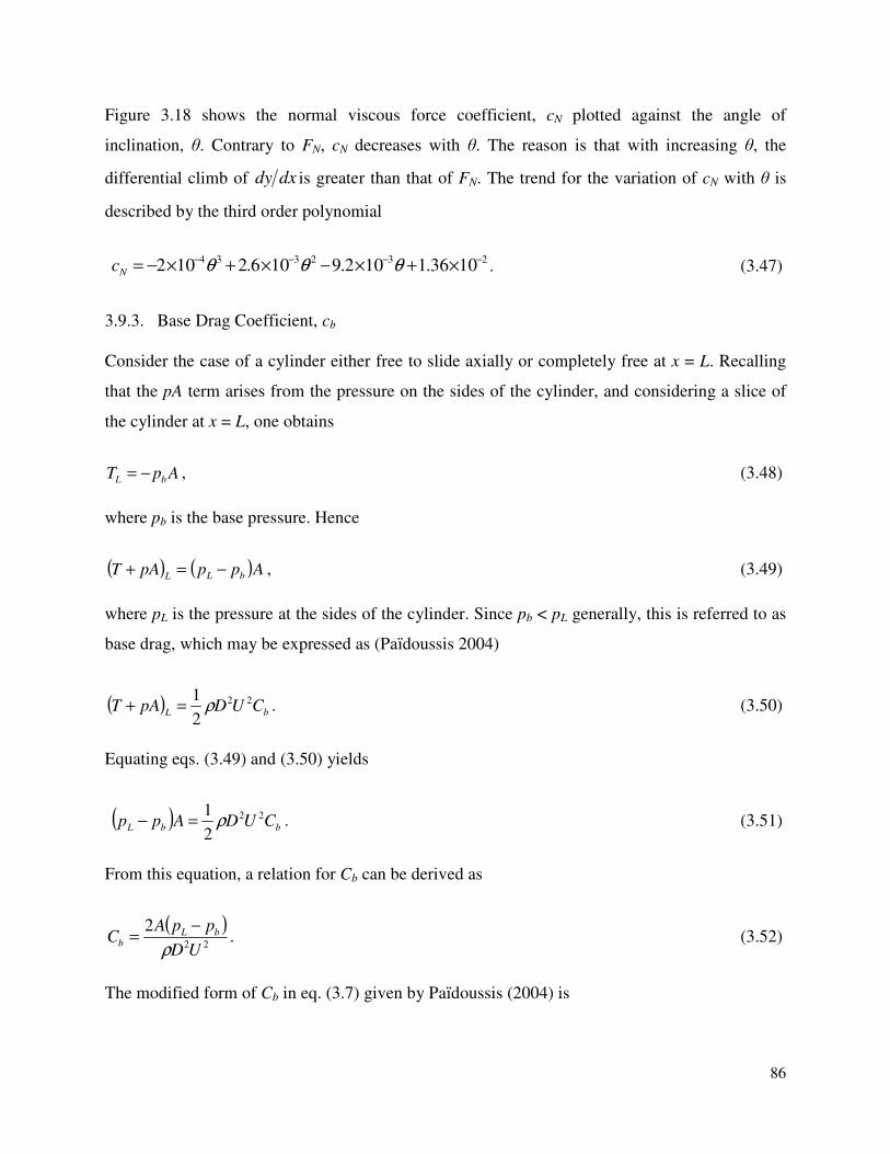
86
Figure 3.18 shows the normal viscous force coefficient, cN plotted against the angle of
inclination, θ. Contrary to FN, cN decreases with θ. The reason is that with increasing θ, the
differential climb of dxdy is greater than that of FN. The trend for the variation of cN with θ is
described by the third order polynomial
232334 1036.1102.9106.2102 −−−− ×+×−×+×−= θθθNc . (3.47)
3.9.3. Base Drag Coefficient, cb
Consider the case of a cylinder either free to slide axially or completely free at x = L. Recalling
that the pA term arises from the pressure on the sides of the cylinder, and considering a slice of
the cylinder at x = L, one obtains
ApT bL −= , (3.48)
where pb is the base pressure. Hence
( ) ( )ApppAT bLL−=+ , (3.49)
where pL is the pressure at the sides of the cylinder. Since pb < pL generally, this is referred to as
base drag, which may be expressed as (Paїdoussis 2004)
( )bL
CUDpAT 22
2
1ρ=+ . (3.50)
Equating eqs. (3.49) and (3.50) yields
( ) bbL CUDApp 22
2
1ρ=− . (3.51)
From this equation, a relation for Cb can be derived as
( )22
2
UD
ppAC bL
bρ
−= . (3.52)
The modified form of Cb in eq. (3.7) given by Paїdoussis (2004) is
87
bb Ccπ
4= . (3.53)
Many researchers have calculated the base drag coefficient cb for various base- and
forebody-shapes in the past (Hoerner 1965; Idel’ chik 1966; Blevins 1984). Based on the
formulation of Hoerner (1965), Paїdoussis (2004) obtained cb = 0.21 for a blunt end forebody
and 1.17 for a hemispherical end with no forebody. Based on the past obtained values of cb,
Paїdoussis (2004) suggested a reasonable range as 0.1 < cb < 0.7.
Consider eq. (3.52) with known input parameters A = 5.0671×10⁻⁴
m2, ρ = 998.2 kg/m
3,
and D = 0.0254 m. The parameters such as pL and pb are determined by developing a rigid
cylinder model at zero angle of inclination in ADINA as shown in Fig. 3.19. The total number of
elements in the numerical fluid domain is 73483. Although Fig. 3.19 is similar to Fig. 3.13 but
included for the sake of the representation of the model to determine pressures independent of
the previous sections. Simulations are performed for U (m/s) = 0.321, 0.640, 0.960, 1.280, 1.603
and ε = 5, 10, 15, 20, 30, 40, 50. The corresponding dimensionless flow velocities u are 0.5, 1.0,
1.5, 2.0, 2.5 and Reynolds numbers Re are 6.5×10⁴, 1.3×10
5, 1.9×10
5, 2.6×10
5, 3.2×10
5.The
values of pL and pb for each U and ε are substituted in eq. (3.52) to obtain Cb. The corresponding
modified values of cb are obtained by substituting the values of Cb in eq. (3.53). Finally, the
mean value of cb obtained is 0.2024, which is well within the suggested range by Paїdoussis
(2004).
Figure 3.20 shows the base drag coefficient, cb, plotted against ε for different values of
dimensionless flow velocity u. The general trend shows that with growing ε at a certain flow
velocity u, cb decreases. The possible reason for this trend is that, due to boundary layer
development along the length of the cylinder, the average pressure at the sides of the cylinder
decreases for larger ε, causing the difference between pL and pb to decrease. The eventual result
comes in the form of reduced cb. Figure 3.21 shows cb versus u at different values of ε.
Increasing the flow velocity, u at certain ε causes the average pressure at the sides of the cylinder
to increase and eventually leads to widening the gap between the value of pL and pb. This causes
the value of cb to increase. In Fig. 3.20, a peculiar peak in the value of cb at ε = 1.5 is quite
obvious. From the results, it is observed that the base pressure first starts decreasing with
increasing ε. From ε = 10 to 15, a sudden drop in the value of pb is observed. After that pb starts
increasing. (pL - pb), which is a major parameter in the determination of cb results in a higher
88
value at ε =1.5 due that sudden drop. It might be a threshold value of ε after that the base
pressure starts increasing. But still the exact reason is not clear. Figure 3.22 shows the plot of
average cb versus u depicting this increasing trend.
It is important to note that all the plots in Sections 3.9.1, 3.9.2, and 3.9.3 cannot have
smooth lines as the calculations involve the results from the ADINA simulations, which can be
considered as numerical experiments generating discrete values.
3.9.4. Zero-Flow Normal Coefficient, c
Recalling eq. (3.42), the second term stands for a linear mean contribution of the quadratic
viscous forces at no fluid flow velocity. This term is retained, since all other viscous force terms
disappear at U = 0 (Chen and Wambsganss 1972). Here, CD is not dimensionless (Paїdoussis
2004); it has the units of velocity. The final form of eq. (3.42) thus obtained is
t
yDCF D
∂
∂= ρ
2
1. (3.54)
The drag coefficient for a long cylinder oscillating in quiescent viscous fluid has been
discussed by Paїdoussis (1998). The viscous force per unit length is found to be given by
Ω−=
dt
dzACF
dρ , (3.55)
where z is the displacement, Ω the radian frequency, ρ the fluid density, A the cylinder cross-
sectional area, and Cd the drag coefficient. Comparing eqs. (3.54) and (3.55) gives the expression
for CD as
dDCDC Ω
=
2
π. (3.56)
In order to render CD dimensionless, Paїdoussis (2004) derived the following expression
DLCEI
Ac
214
=
ρ
π. (3.57)
89
Paїdoussis (2004) considered two cases in order to establish reasonable range of c. He
obtained a lower value of c equal to 0.008 by considering a cylinder made of metal and a higher
value equal to 0.06 by considering an elastomer cylinder. Sinyavskii et al. (1980) derived the
expression for Cd as
( )
,1
12222
3
c
cd
StkC
γ
γ
−
+= (3.58)
where γc is the confinement parameter given by the expression
,ch
cR
R=γ (3.59)
where R and Rch are the cylinder and channel radii, respectively. Consider the case with no
confinement. In this case, γc = 0 and the resulting expression for Cd obtained is
.22
StkCd = (3.60)
This is the same expression derived by Batchelor (1967); Stk is Stokes number given by
.2
k
RStk
ν
Ω= (3.61)
In order to calculate Ω, the expression given by Paїdoussis (2004) is used, which is
2
21
LEI
mAΩ
+=
ρω , (3.62)
where ω is the dimensionless complex frequency and m is the mass of cylinder per unit length.
Re-ordering of eq. (3.62) gives
21
2
+=Ω
mA
EI
L ρ
ω. (3.63)

90
In order to determine ω, a MATLAB code to solve the linear equation of motion for a
cantilevered cylinder with system parameters D = 0.0254 m, ρ = 998.2 kg/m3, E = 2.76×10
6 Pa, I
= 2.0432×10⁻⁸
m4, L = 0.52 m, νk = 1.004×10
-6 m
2/s, and m = 0.5675 kg/m are employed. These
parameters match the experimental ones. The iterative solution starts by considering an initial
guess for c equal to zero in the code. From the solution, ω at the critical value of cylinder second
mode instability, i.e., flutter, is obtained; ω is the real part of the complex eigenfrequency. The
value of ω is substituted in eq. (3.63) to obtain Ω, which is, in turn, put in eq. (3.61) to get St.
Hereafter, eqs. (3.60), (3.56) and (3.57) are used in order to obtain the value of c. The obtained
value of c is plugged in the MATLAB code to obtain new values of ω, Ω, Stk, Cd, CD, and finally
c. This procedure is repeated until a converged value of c is obtained. From the above mentioned
procedure, the value of c thus obtained is 0.0510, which is within the range 0.008 ≤ c ≤ 0.060,
proposed by Paїdoussis (2004).
3.10. Model in Water Flow with Presently Calculated Force Coefficients
3.10.1. Adequacy of the Linear Solution
Adequacy of the linear solution with the presently calculated force coefficients is established by
solving the linear equation especially for this purpose and comparing the critical flow velocity
for the onset of first mode divergence, ucr,d1, with the experimental one. The solution of the linear
equation yields ucr,d1 = 1.904. The measured critical flow velocity, ucr,d1, in experiments is 1.87
(Chapter 2). The difference is 1.81%, which is in good agreement.
3.10.2. Analytical Results
The presently obtained force coefficients are substituted in the linear equation of motion for
cantilevered flexible cylinder in water flow and solved using MATLAB code. The values of
these force coefficients and other parameters are: β = 0.5, εcN = 0.0852, εcT = 0.4857, f = 0.8, χ =
1, εc = 1.0571, cb = 0.2024, ε = 20.7283, γ = 1.23, and δ = α = Γ = 0. The results (Fig. 3.23) show
that cylinder motions if caused by perturbation are damped at small u. As velocity is increased,
the complex frequency becomes purely imaginary with zero frequency but remains positive,
indicating that the cylinder displacement is damped. At sufficiently high u, however, the cylinder
first loses stability by divergence in its first mode, via a pitchfork bifurcation, at ucr,d1 = 1.904.
91
The critical velocity ucr,d1 is marked by the imaginary branch of the complex frequency
becoming negative along the Im(ω)-axis at zero frequency. At higher flow velocity, the cylinder
re-stabilizes in its first mode at ur1 = 5.237. Before u1 is reached, the cylinder second mode in
stable region bifurcates on Im(ω)-axis at u2,0 = 4.921. The dimensionless flow velocity u2,0
signifies the velocity corresponding to zero frequency of the second mode-shape locus along
positive Im(ω)-axis in the stable region. At slightly higher velocity, u1,2 = 5.243, the positive
branches of the first and second mode loci coalesce and leave the axis at a point where Im(ω) >
0, indicating the motions damped out. Soon after, at ucr,fl1,2 = 5.278, the imaginary branches of
the couple mode loci become negative, i.e., Im(ω) < 0, at a finite frequency, indicating the onset
of coupled-mode flutter. The corresponding value of Re(ωcr,fl1,2) is equal to 3.92. The cylinder
does not become unstable in the third mode, even at higher velocities as high as u = 12. Figures
3.24 and 3.25 show the frequency and damping plotted against the dimensionless velocity u.
3.11. Effect of Confinement
Next, the effect of confinement on the critical value of u for the onset of divergence and flutter of
cantilevered cylinder in water flow is analyzed with the presently calculated force coefficients
substituted in the model’s MATLAB code. The results of the critical values of flow velocity for
the onset of divergence and coupled-mode flutter varying with confinement are shown in Figs.
3.26 and 3.27, respectively for 1.01 ≤ χ ≤ 2.00. With increasing confinement, viscous effects
become more pronounced and the stream wise pressure drop acquires considerable value. This
results in the divergence and coupled-mode flutter of the cylinder occurring earlier with
increasing flow velocity.
3.12. Comparison of the Results
The results using the previously used force coefficients (Paїdoussis 1973) are compared with
those of Paїdoussis (1973). Paїdoussis (1973) solved the equations of motion by considering a
solution of the form
( ) ( ) ωτξτξη ieY=, . (3.64)
92
For a cantilevered cylinder, he expanded Y(ξ) in terms of a power series in ξ. The procedure to
solve the present model has already been described above. Table 3.2 shows the comparison of
cantilevered cylinder results with those of Paїdoussis (1973). Results are in good agreement.
Table 3.3 presents the comparison of cantilevered cylinder critical velocities and the
corresponding dimensionless frequencies with previously used force coefficients by Paїdoussis
(1973) and presently calculated ones. With the presently calculated force coefficients, lower ucr,d1
are obtained than with the previous force coefficients; also coupled-mode flutter is obtained
instead of a single mode flutter. The reason can be understood by considering the effects of f and
cb on the dynamics of the cylinder. According to theory, decreasing f stabilizes the system for
divergence, while increasing cb destabilizes it. Since the model with the present force
coefficients has same value of f (0.8) and a higher value of cb (0.2024) than the one with previous
coefficients (cb = 0.0), the results suggest that the effect of cb makes the cylinder statically
unstable at lower ucr,d1. For flutter, theory predicts that decreasing f and increasing cb both have a
stabilizing effect. This is exactly what is observed in the table with ucr,fl1,2 being higher for the
model with present coefficients. Third mode flutter is not observed for the model with present
force coefficients. Since the results show, in general, a higher critical flow velocity for flutter,
this may lead to the occurrence of third mode flutter at a dimensionless flow velocity higher than
u = 12, which is the maximum velocity used in the code. The results of the linear model for the
cantilevered cylindrical system with the presently calculated force coefficients demonstrate
similar dynamics as observed in the experiments, especially the coalesced first mode divergence
and second mode flutter as the coupled-mode flutter (combination of the two modes leads to an
asymmetric response also observed in Figs. 2.32 and 2.33 in Chapter 2). Hence, it can be stated
that the linear model with the presently calculated force coefficients predicts the dynamics of the
system better than the one with the previously used force coefficients.
Table 3.4 presents the comparison of critical velocities of cantilevered cylinder in water
and air flows employing the previous force coefficients. Considering the models in water and air
flows, it is seen that ucr,d1 is the same for both models, which means that divergence is
independent of β, as observed by Paїdoussis (2004). However, a drop in ucr,fl2 for the model in air
flow can be seen. This is due to the inherent lower viscous damping of air. This also enables the
cylinder in air flow to oscillate with higher frequency. In addition, the cylinder does not develop
third mode flutter in air flow up to the maximum dimensionless flow velocity, i.e., u = 12, used
93
in the code. It may be inferred that the energy transfer from air to the cylinder is not sufficient
enough to excite it in third mode.
3.13. Summary
In this chapter, after the general introduction of the problem under consideration, two-
dimensional linear equations of motion, governing the cantilevered cylinder dynamics, in
dimensional and dimensionless forms, and the methods of solution were presented followed by
the solutions of the models in water flow using the MATLAB code. The mass ratio was then
modified for the cantilevered cylinder case in air flow. Effects of confinement on the dynamics
of cantilevered cylinder in water and air flows were then studied. Force coefficients present in
the equation of motion were then recalculated based on the present geometrical and flow
parameters matching the experimental ones, and with the presently calculated coefficients, the
equations of motion were solved again for the cantilevered cylinder model using MATLAB
code. Finally, the model results were compared with the ones available in the literature and with
each other.
First, the general equation of motion with the boundary conditions for cantilevered
cylinder was presented followed by its dimensionless form. In order to transform or simplify the
two-dimensional fourth order linear Partial Differential Equations (PDE) into second order
Ordinary Differential Equation (ODE), extended Galerkin method was used due to its time
dependent free end boundary condition. The ODE was further simplified to a first order
eigenvalue problem. It was then solved for a range of flow velocities using a MATLAB code and
the respective results were presented. The present code for cantilevered cylinder was then run for
air flow by modifying the mass ratio, β, and the results were presented. Results pertaining to the
effects of confinement on the critical velocities for cantilevered cylinder in water and air flows
were later presented.
Force coefficients such as longitudinal viscous coefficient, cT, normal viscous coefficient,
cN, base drag coefficient, cb, and zero-flow normal coefficient, c, were recalculated based on the
present physical parameters matching the experiment conditions. After substituting the presently
calculated coefficients in the MATLAB code, solution for the cantilevered cylinder in water flow
was obtained. Similarly, the effect of confinement on the critical velocities for cantilevered
cylinder was then presented.
94
Finally, three sets of comparison were done. The first set compared the critical flow
velocities for cantilevered cylinder obtained in the present model by using the previously used
force coefficients with the ones in the literature. The second set compared the critical flow
velocities using the previous force coefficients with the ones obtained by using the present force
coefficients. The third set compared the critical flow velocities for the cantilevered cylinder in
water flow with the ones in air flow.
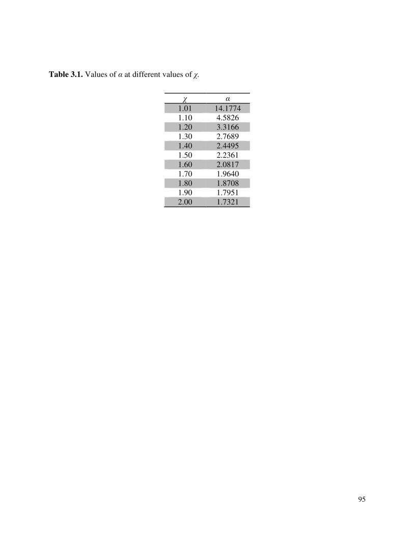
95
Table 3.1. Values of α at different values of χ.
χ α
1.01 14.1774
1.10 4.5826
1.20 3.3166
1.30 2.7689
1.40 2.4495
1.50 2.2361
1.60 2.0817
1.70 1.9640
1.80 1.8708
1.90 1.7951
2.00 1.7321
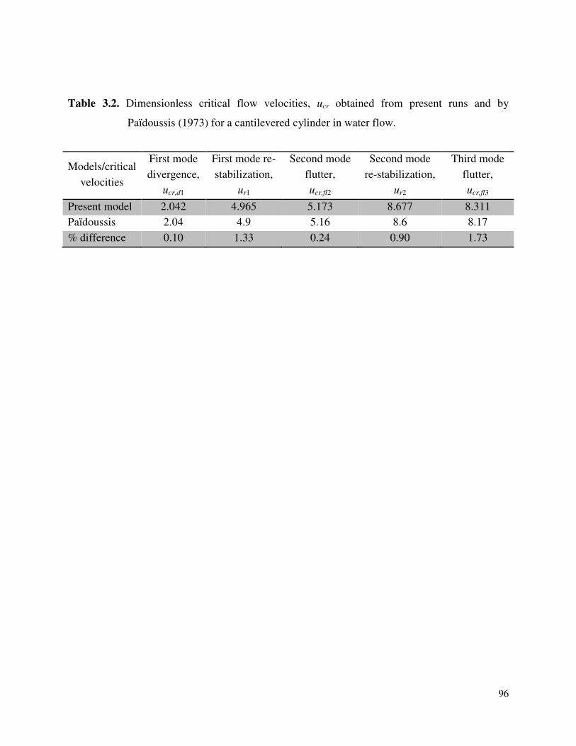
96
Table 3.2. Dimensionless critical flow velocities, ucr obtained from present runs and by
Paїdoussis (1973) for a cantilevered cylinder in water flow.
Models/critical
velocities
First mode
divergence,
ucr,d1
First mode re-
stabilization,
ur1
Second mode
flutter,
ucr,fl2
Second mode
re-stabilization,
ur2
Third mode
flutter,
ucr,fl3
Present model 2.042 4.965 5.173 8.677 8.311
Paїdoussis 2.04 4.9 5.16 8.6 8.17
% difference 0.10 1.33 0.24 0.90 1.73
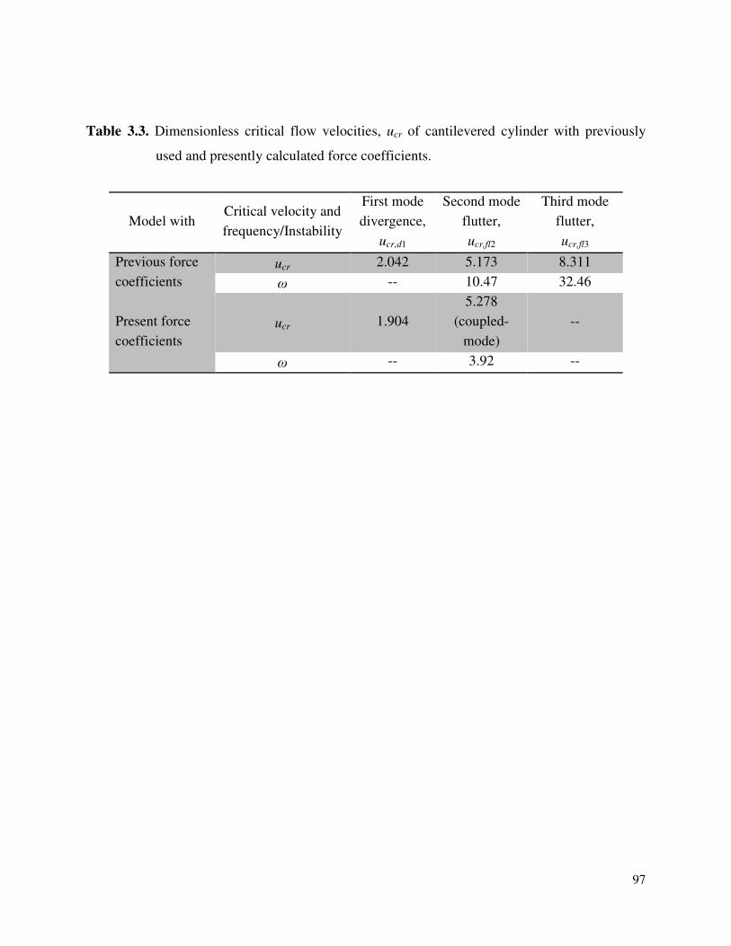
97
Table 3.3. Dimensionless critical flow velocities, ucr of cantilevered cylinder with previously
used and presently calculated force coefficients.
Model with Critical velocity and
frequency/Instability
First mode
divergence,
ucr,d1
Second mode
flutter,
ucr,fl2
Third mode
flutter,
ucr,fl3
Previous force
coefficients
ucr 2.042 5.173 8.311
ω -- 10.47 32.46
Present force
coefficients
ucr 1.904
5.278
(coupled-
mode)
--
ω -- 3.92 --
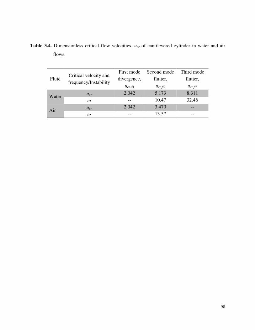
98
Table 3.4. Dimensionless critical flow velocities, ucr of cantilevered cylinder in water and air
flows.
Fluid Critical velocity and
frequency/Instability
First mode
divergence,
ucr,d1
Second mode
flutter,
ucr,fl2
Third mode
flutter,
ucr,fl3
Water ucr 2.042 5.173 8.311
ω -- 10.47 32.46
Air ucr 2.042 3.470 --
ω -- 13.57 --

99
Fig. 3.1. (a) Schematic diagram of a flexible cylinder in a confined vertical axial flow (b)
Diagrammatic view of a cantilevered cylinder in axial flow in the test-section of a
circulating system.
Flexible cantilevered cylinder
Rch
R
U
g
(a) (b)
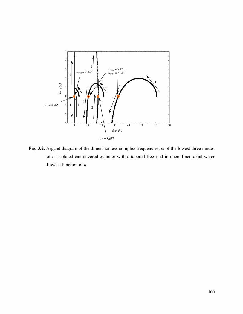
100
Fig. 3.2. Argand diagram of the dimensionless complex frequencies, ω of the lowest three modes
of an isolated cantilevered cylinder with a tapered free end in unconfined axial water
flow as function of u.
ur2 = 8.677
ucr,fl2 = 5.173;
ucr,fl3 = 8.311
2
2
3
3
1
1
1
1 2
2
ucr,d1 = 2.042
ur1 = 4.965
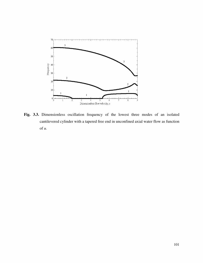
101
Fig. 3.3. Dimensionless oscillation frequency of the lowest three modes of an isolated
cantilevered cylinder with a tapered free end in unconfined axial water flow as function
of u.
1 1
1
2
2
3
3
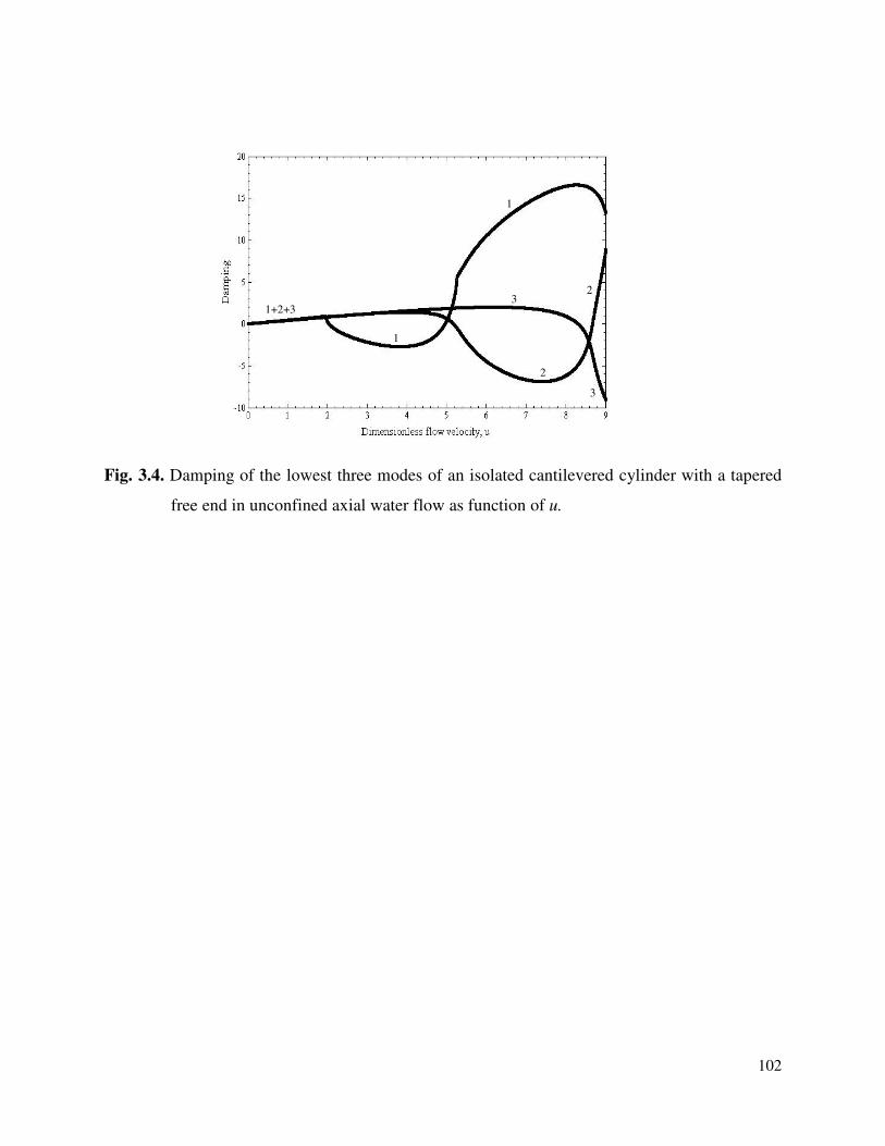
102
Fig. 3.4. Damping of the lowest three modes of an isolated cantilevered cylinder with a tapered
free end in unconfined axial water flow as function of u.
3
3
1
1
2
2
1+2+3
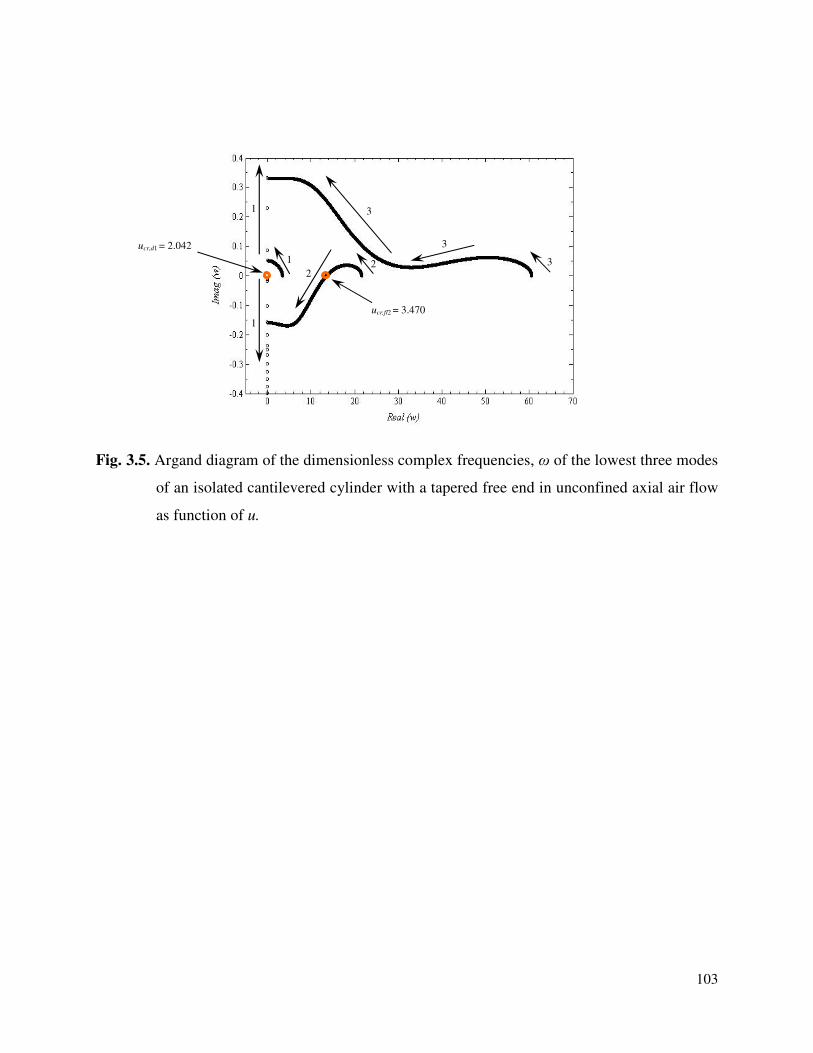
103
Fig. 3.5. Argand diagram of the dimensionless complex frequencies, ω of the lowest three modes
of an isolated cantilevered cylinder with a tapered free end in unconfined axial air flow
as function of u.
2 2
1
1
1
3
3
ucr,fl2 = 3.470
3
ucr,d1 = 2.042
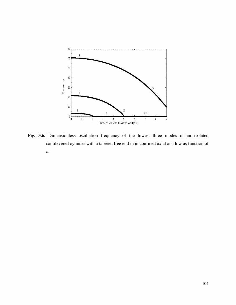
104
Fig. 3.6. Dimensionless oscillation frequency of the lowest three modes of an isolated
cantilevered cylinder with a tapered free end in unconfined axial air flow as function of
u.
2
1 1
2 1+2
3
3
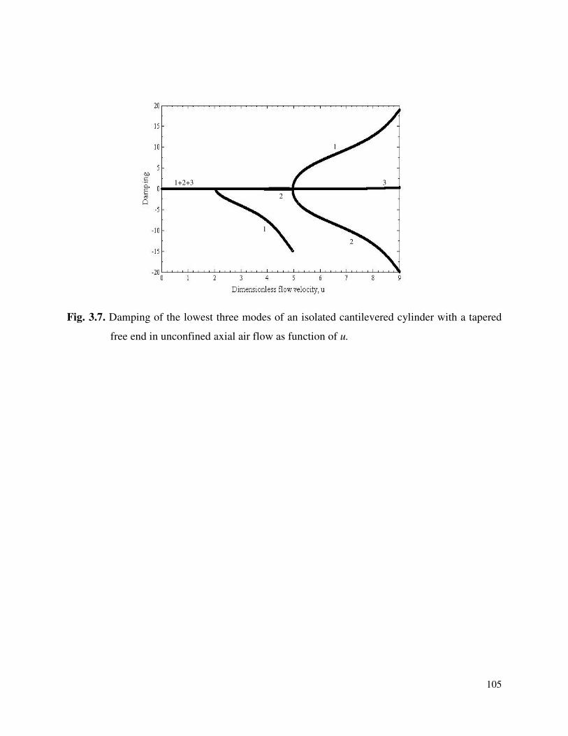
105
Fig. 3.7. Damping of the lowest three modes of an isolated cantilevered cylinder with a tapered
free end in unconfined axial air flow as function of u.
3
2
2
1
1
1+2+3
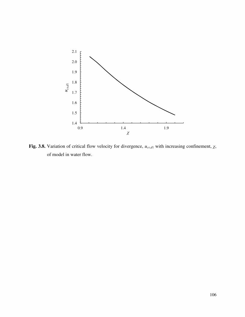
106
Fig. 3.8. Variation of critical flow velocity for divergence, ucr,d1 with increasing confinement, χ,
of model in water flow.
1.4
1.5
1.6
1.7
1.8
1.9
2.0
2.1
0.9 1.4 1.9
ucr,
d1
χ
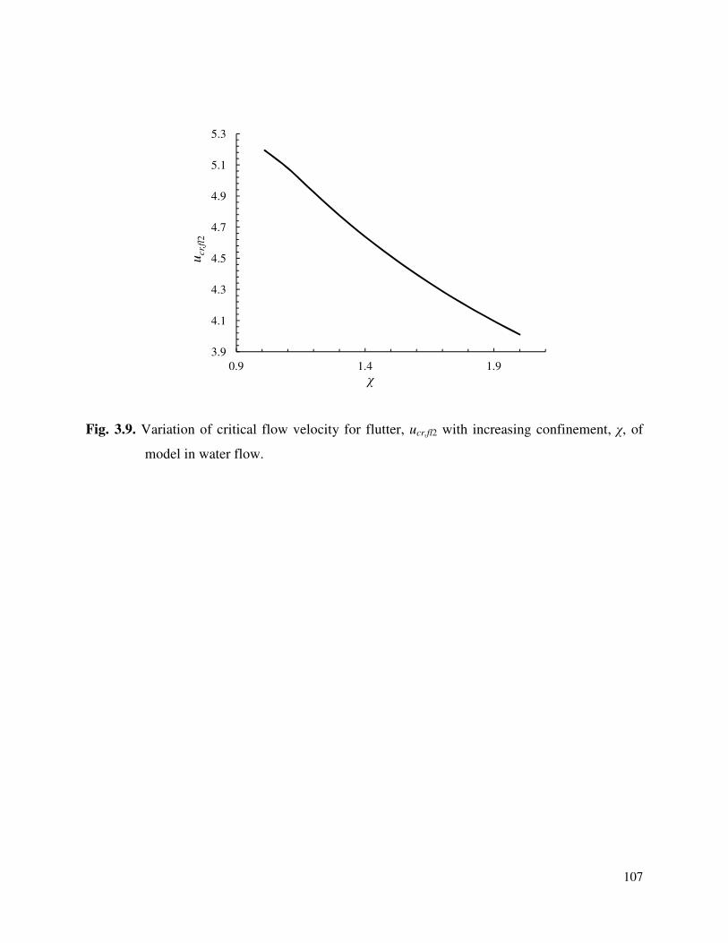
107
Fig. 3.9. Variation of critical flow velocity for flutter, ucr,fl2 with increasing confinement, χ, of
model in water flow.
3.9
4.1
4.3
4.5
4.7
4.9
5.1
5.3
0.9 1.4 1.9
ucr,
fl2
χ
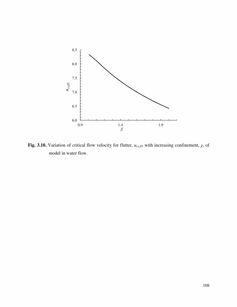
108
Fig. 3.10. Variation of critical flow velocity for flutter, ucr,fl3 with increasing confinement, χ, of
model in water flow.
6.0
6.5
7.0
7.5
8.0
8.5
0.9 1.4 1.9
ucr,
fl3
χ
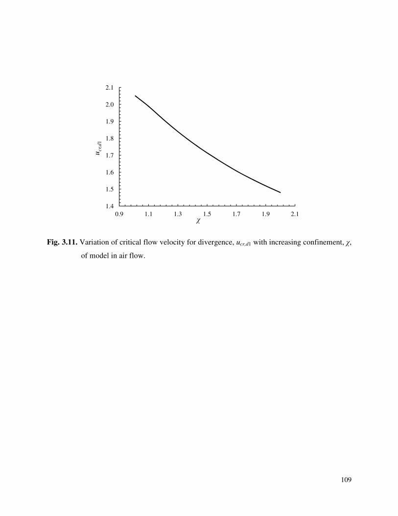
109
Fig. 3.11. Variation of critical flow velocity for divergence, ucr,d1 with increasing confinement, χ,
of model in air flow.
1.4
1.5
1.6
1.7
1.8
1.9
2.0
2.1
0.9 1.1 1.3 1.5 1.7 1.9 2.1
ucr,
d1
χ
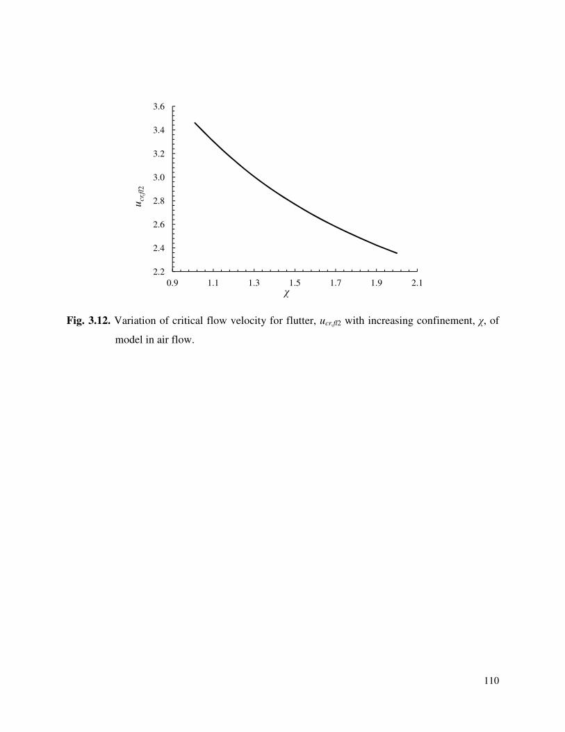
110
Fig. 3.12. Variation of critical flow velocity for flutter, ucr,fl2 with increasing confinement, χ, of
model in air flow.
2.2
2.4
2.6
2.8
3.0
3.2
3.4
3.6
0.9 1.1 1.3 1.5 1.7 1.9 2.1
ucr,
fl2
χ
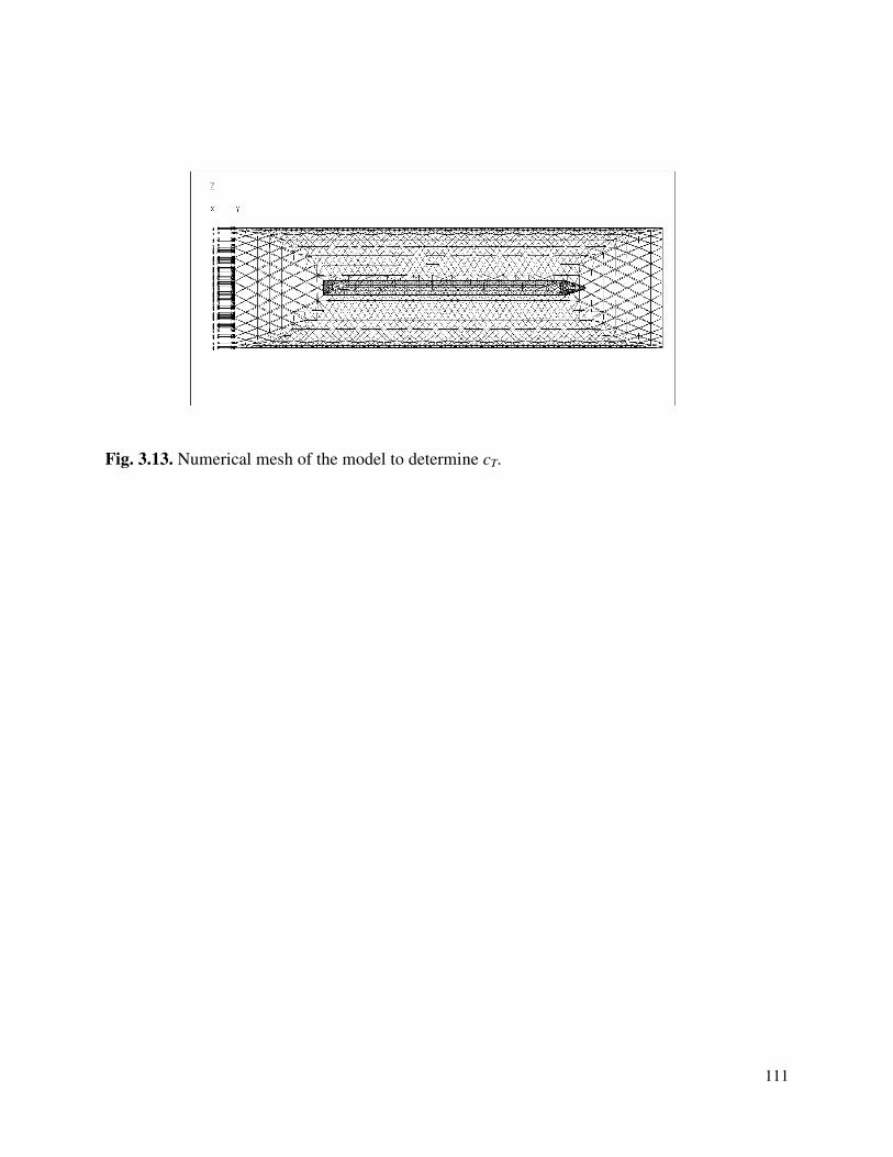
111
Fig. 3.13. Numerical mesh of the model to determine cT.
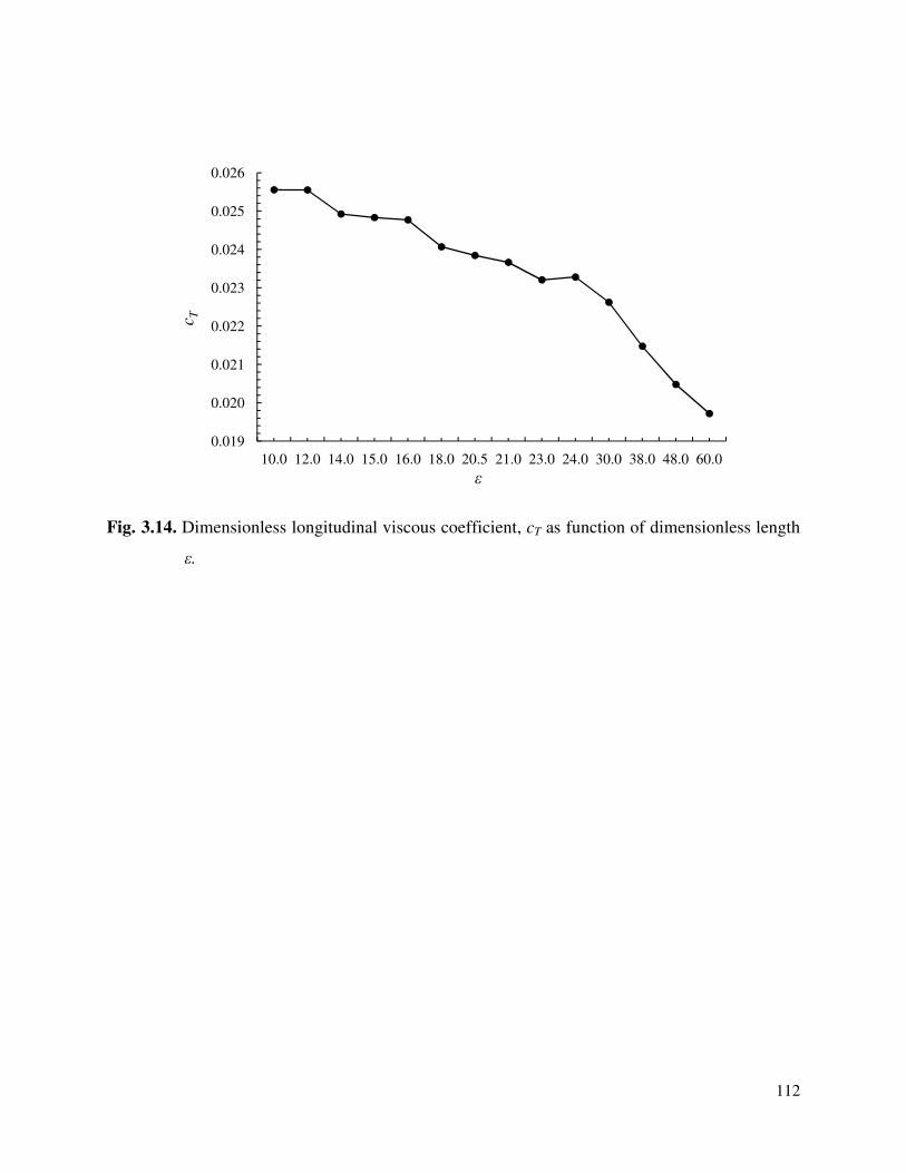
112
Fig. 3.14. Dimensionless longitudinal viscous coefficient, cT as function of dimensionless length
ε.
0.019
0.020
0.021
0.022
0.023
0.024
0.025
0.026
10.0 12.0 14.0 15.0 16.0 18.0 20.5 21.0 23.0 24.0 30.0 38.0 48.0 60.0
c T
ε
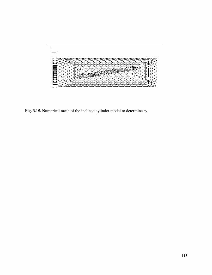
113
Fig. 3.15. Numerical mesh of the inclined cylinder model to determine cN.
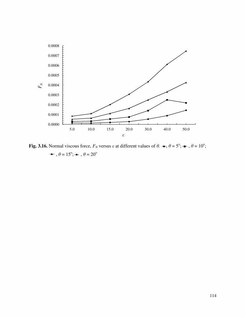
114
Fig. 3.16. Normal viscous force, FN versus ε at different values of θ. , θ = 5o; , θ = 10
o;
, θ = 15o; , θ = 20
o
0.0000
0.0001
0.0002
0.0003
0.0004
0.0005
0.0006
0.0007
0.0008
5.0 10.0 15.0 20.0 30.0 40.0 50.0
FN
ε
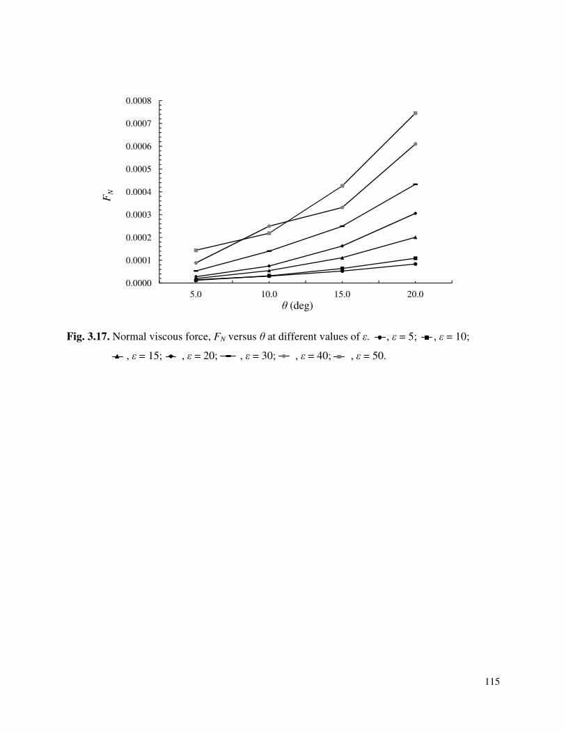
115
Fig. 3.17. Normal viscous force, FN versus θ at different values of ε. , ε = 5; , ε = 10;
, ε = 15; , ε = 20; , ε = 30; , ε = 40; , ε = 50.
0.0000
0.0001
0.0002
0.0003
0.0004
0.0005
0.0006
0.0007
0.0008
5.0 10.0 15.0 20.0
FN
θ (deg)
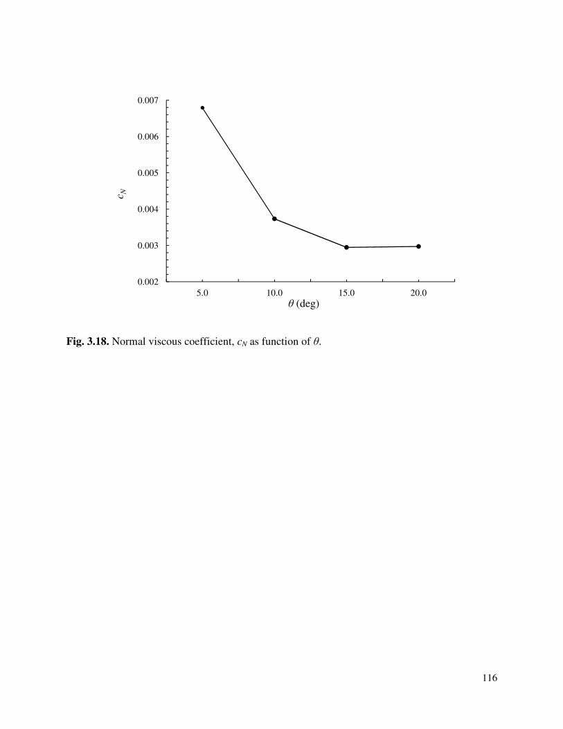
116
Fig. 3.18. Normal viscous coefficient, cN as function of θ.
0.002
0.003
0.004
0.005
0.006
0.007
5.0 10.0 15.0 20.0
c N
θ (deg)
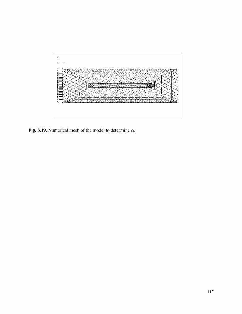
117
Fig. 3.19. Numerical mesh of the model to determine cb.

118
Fig. 3.20. Base drag coefficient, cb versus ε at different values of u. , u = 0.5; , u = 1.0;
, u = 1.5; , u = 2.0; , u = 2.5
0.10
0.15
0.20
0.25
0.30
5.0 10.0 15.0 20.0 30.0 40.0 50.0
c b
ε
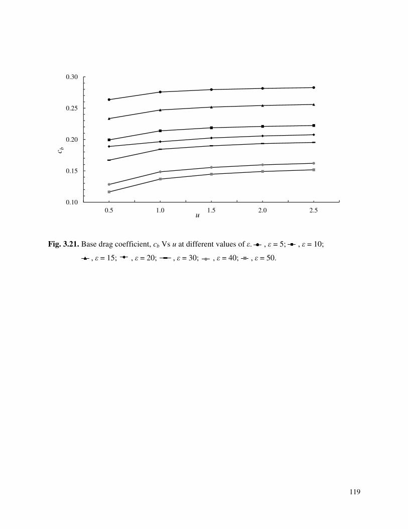
119
Fig. 3.21. Base drag coefficient, cb Vs u at different values of ε. , ε = 5; , ε = 10;
, ε = 15; , ε = 20; , ε = 30; , ε = 40; , ε = 50.
0.10
0.15
0.20
0.25
0.30
0.5 1.0 1.5 2.0 2.5
c b
u
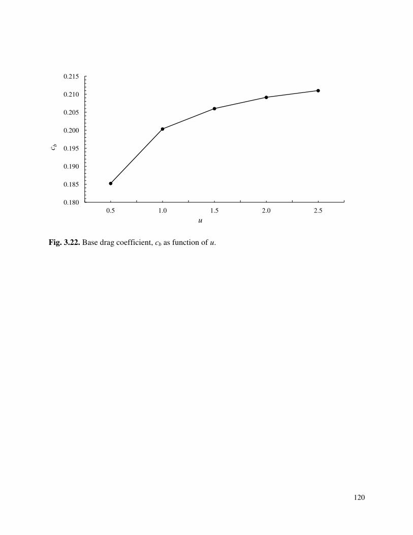
120
Fig. 3.22. Base drag coefficient, cb as function of u.
0.180
0.185
0.190
0.195
0.200
0.205
0.210
0.215
0.5 1.0 1.5 2.0 2.5
c b
u
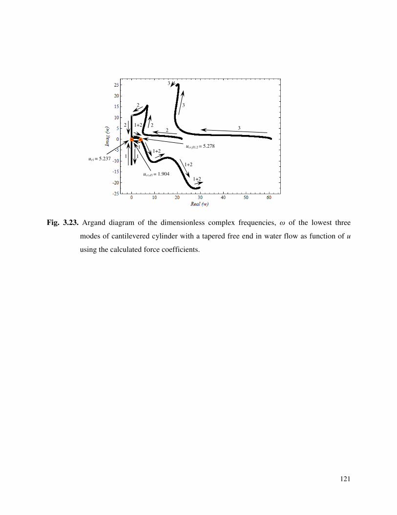
121
Fig. 3.23. Argand diagram of the dimensionless complex frequencies, ω of the lowest three
modes of cantilevered cylinder with a tapered free end in water flow as function of u
using the calculated force coefficients.
1
1 1
2 2
2
2 3
3
3
1+2
1+2
1+2
1+2 ucr,d1 = 1.904
ur1 = 5.237
ucr,fl1,2 = 5.278
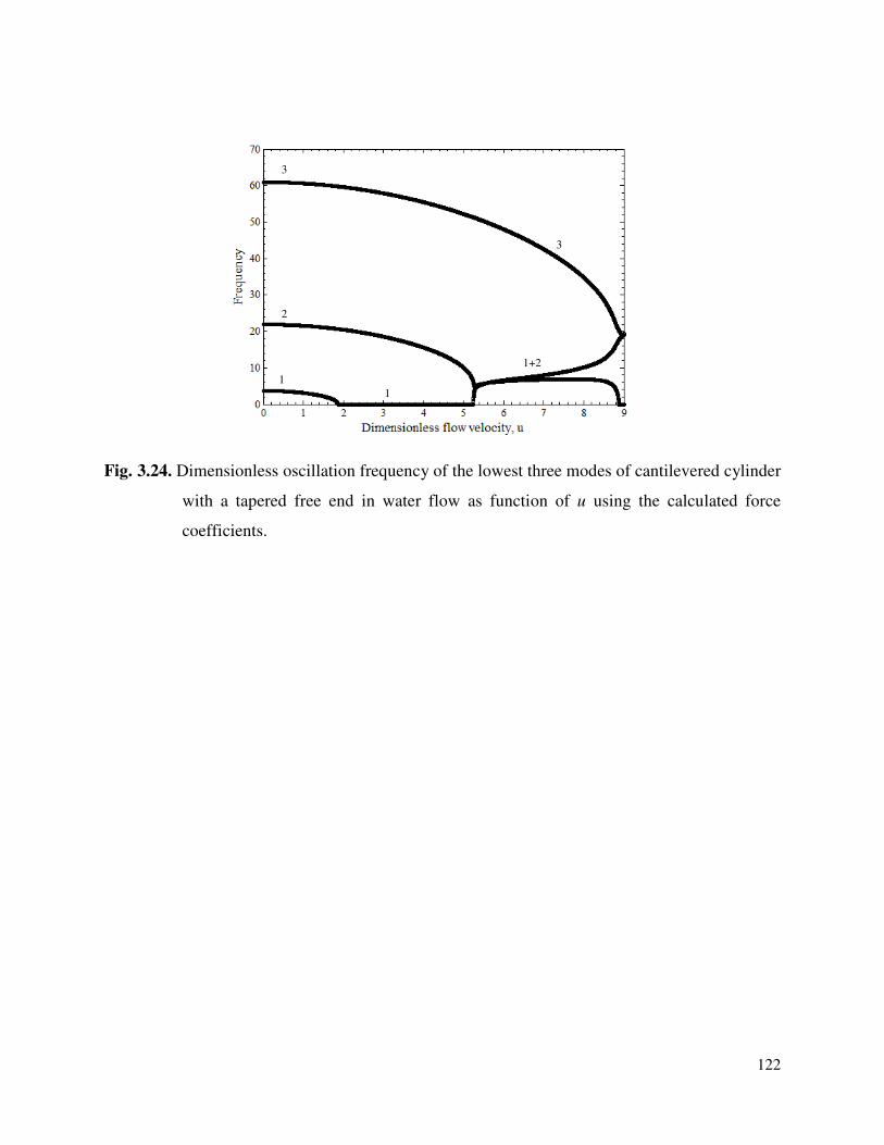
122
Fig. 3.24. Dimensionless oscillation frequency of the lowest three modes of cantilevered cylinder
with a tapered free end in water flow as function of u using the calculated force
coefficients.
1
1
2
3
3
1+2
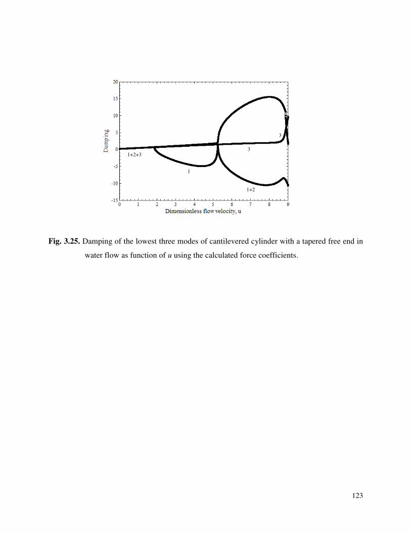
123
Fig. 3.25. Damping of the lowest three modes of cantilevered cylinder with a tapered free end in
water flow as function of u using the calculated force coefficients.
3
3
1+2
1
1+2+3
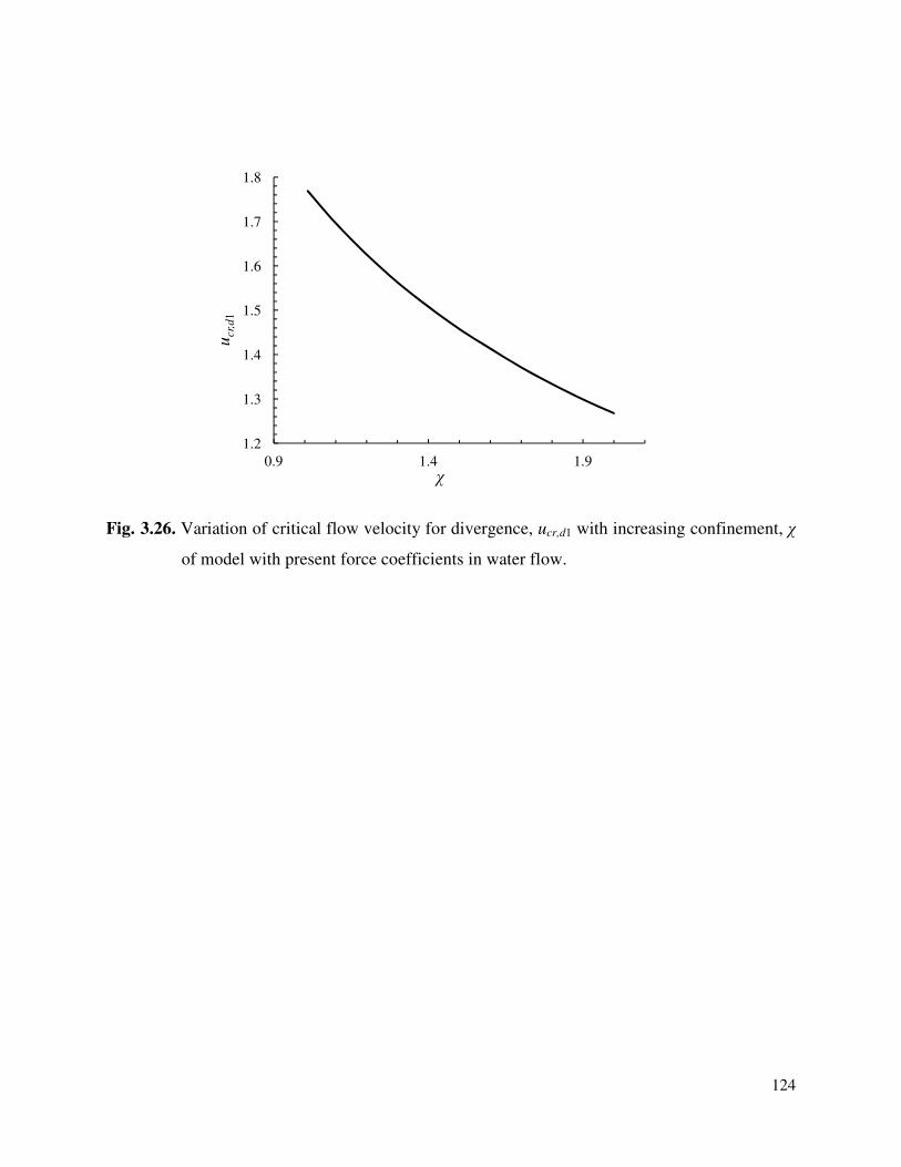
124
Fig. 3.26. Variation of critical flow velocity for divergence, ucr,d1 with increasing confinement, χ
of model with present force coefficients in water flow.
1.2
1.3
1.4
1.5
1.6
1.7
1.8
0.9 1.4 1.9
ucr,
d1
χ
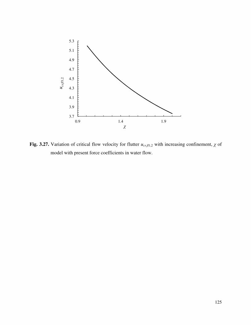
125
Fig. 3.27. Variation of critical flow velocity for flutter ucr,fl1,2 with increasing confinement, χ of
model with present force coefficients in water flow.
3.7
3.9
4.1
4.3
4.5
4.7
4.9
5.1
5.3
0.9 1.4 1.9
ucr,
fl1
,2
χ
Chapter 4
Nonlinear Analysis
4.1. Introduction
As established earlier, a linear model can reliably predict the first point of instability of a flexible
cylinder in axial flow, which is most of the time divergence (a static instability). The post-
divergence dynamics of the cylinder, however, has to be confirmed through a nonlinear model
(Paїdoussis 1998, 2004; Modarres-Sadeghi 2006). It is also noted in the previous research work,
presented in Chapter 1, utilizing the nonlinear models to describe the system dynamics of
flexible slender cylinder in axial flow (Paїdoussis et al. 2002; Modarres-Sadeghi 2005, 2007), the
force coefficients were either chosen from a reasonable range or determined based on some
simple relations. Therefore, there is a need to solve the nonlinear equation with the force
coefficients, calculated in Chapter 3, incorporated in it in order to predict the nonlinear dynamics
of the system.
In this Chapter, the dynamic response of a cantilevered cylinder in water flow, is studied
again, this time a described by a nonlinear equation of motion. The system under consideration is
similar to one studied in Chapter 3. The un-deformed cylinder axis coincides with the x-axis. The
cantilevered cylinder is fitted with an ogival end-piece at the free end and considered to be short
relative to the overall length of the cylinder. Furthermore, the fluid is supposed to be contained
by boundaries sufficiently distant from the cylinder to have negligible influence on its motion.
Similar assumptions are considered as in Chapter 3. First, the nonlinear model results are
obtained by utilizing the force coefficients and other input parameters used by Semler et al.
(2002). This is done so as to establish the adequacy of the present numerical method used for the
solution by comparing the obtained results with those by Semler et al. (2002). Secondly, the
presently calculated force coefficients from Chapter 3 are employed in the nonlinear equation
and solved. Finally, the results obtained from the present work with previous and presently
calculated force coefficients are compared with each other in order to see the effect of the force
coefficients on the overall dynamics of the system.
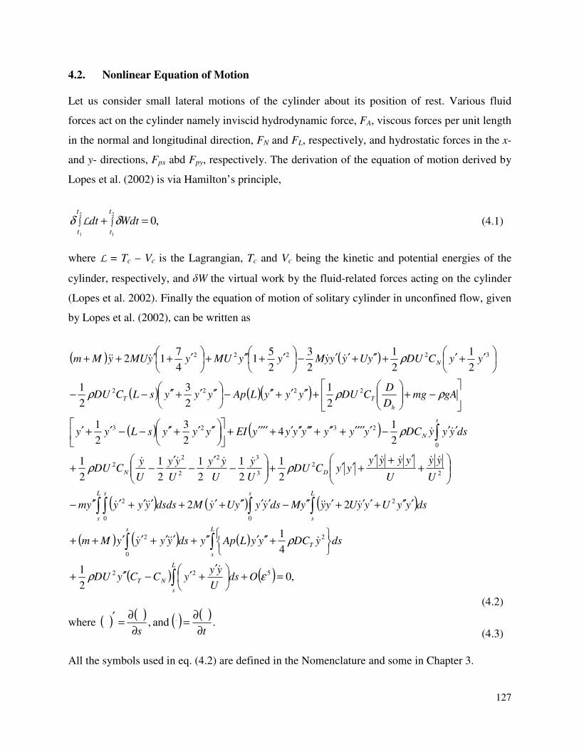
127
4.2. Nonlinear Equation of Motion
Let us consider small lateral motions of the cylinder about its position of rest. Various fluid
forces act on the cylinder namely inviscid hydrodynamic force, FA, viscous forces per unit length
in the normal and longitudinal direction, FN and FL, respectively, and hydrostatic forces in the x-
and y- directions, Fpx abd Fpy, respectively. The derivation of the equation of motion derived by
Lopes et al. (2002) is via Hamilton’s principle,
,02
1
2
1
=+ ∫∫t
t
t
t
Wdtdt δδ L (4.1)
where L = Tc – Vc is the Lagrangian, Tc and Vc being the kinetic and potential energies of the
cylinder, respectively, and δW the virtual work by the fluid-related forces acting on the cylinder
(Lopes et al. 2002). Finally the equation of motion of solitary cylinder in unconfined flow, given
by Lopes et al. (2002), can be written as
( ) ( )
( ) ( )( )
( ) ( )
( ) ( ) ( )
( ) ( ) ( )
( ) ( ) ,02
1
4
1
22
2
1
2
1
2
1
2
1
2
1
2
14
2
3
2
1
2
1
2
3
2
1
2
1
2
1
2
3
2
51
4
712
522
2
0
2
2
0 0
2
2
2
3
32
2
22
0
2323
2222
32222
∫
∫∫
∫∫ ∫ ∫
∫
=+
′+′−′′+
+′′′′′+′′+′′++
′′′+′′+′′′−′′′′+′+′′+′′′−
+
′+′+′′+
−
′−
′−+
′′−′′′′′+′′+′′′′′′+′′′′+
′′′+′′−−′+′
−+
+′′′+′′−
′′′+′′−−
′+′+′′+′′−
′+′′+
′+′++
L
s
NT
L
s
T
s
L
s
L
s
s s
DN
s
N
h
TT
N
OdsU
yyyCCyDU
dsyDCyyLApydsyyyyMm
dsyyUyyUyyyMdsyyyUyMdsdsyyyym
U
yy
U
yyyyyyCDU
U
y
U
yy
U
yy
U
yCDU
dsyyyDCyyyyyyyEIyyysLyy
gAmgD
DCDUyyyLApyyysLCDU
yyCDUyUyyyMyyMUyyMUyMm
ερ
ρ
ρρ
ρ
ρρρ
ρ
&
&&&&
&&&&&&&&
&&&&&&&&
&&
&&&&&
(4.2)
where ( ) ( ) ( ) ( ). and , .
ts ∂
∂=
∂
∂=
′
(4.3)
All the symbols used in eq. (4.2) are defined in the Nomenclature and some in Chapter 3.
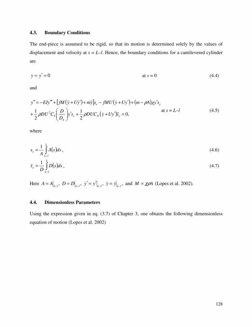
128
4.3. Boundary Conditions
The end-piece is assumed to be rigid, so that its motion is determined solely by the values of
displacement and velocity at s = L–l. Hence, the boundary conditions for a cantilevered cylinder
are
0=′= yy at s = 0 (4.4)
and
( )[ ] ( ) ( )
( ) ,02
1
2
1 2 =′++′
+
′−+′+−+′++′′′−=′′
eNe
h
T
ee
syUyDUCsyD
DCDU
sygAmyUyfMUsymyUyfMyEIy
&
&&&&&&
ρρ
ρ
at s = L–l (4.5)
where
( )∫−
=L
lL
e dssAA
s1
, (4.6)
( )∫−
=L
lL
e dssDD
s1
, (4.7)
Here AMyyyyDDAAlLlLlLlL
χρ==′=′==−−−−
and , , , , && (Lopes et al. 2002).
4.4. Dimensionless Parameters
Using the expression given in eq. (3.7) of Chapter 3, one obtains the following dimensionless
equation of motion (Lopes et al. 2002)
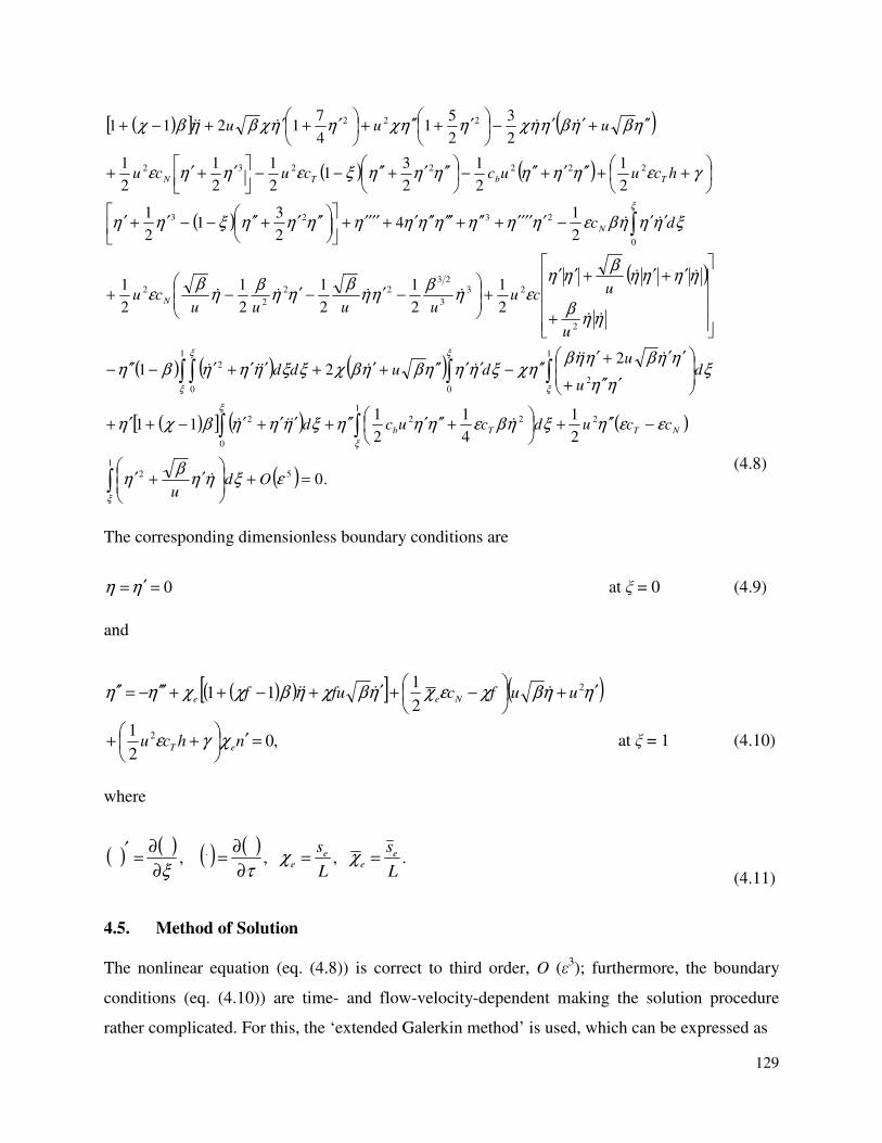
129
( )[ ] ( )
( ) ( )
( )
( )
( ) ( ) ( )
( )[ ] ( ) ( )
( ) .0
2
1
4
1
2
111
221
2
1
2
1
2
1
2
1
2
1
2
14
2
31
2
1
2
1
2
1
2
31
2
1
2
1
2
1
2
3
2
51
4
71211
5
1
2
2
1
22
0
2
1
20
1
0
2
2
23
3
2322
2
2
0
2323
2222232
222
=+
′+′
−′′+
+′′′′′+′′+′−+′+
′′′+
′′+′′′−′′′′+′+′′+′−′′−
+
′+′+′′
+
−′−′−+
′′−′′′′′+′′+′′′′′′+′′′′+
′′′+′′−−′+′
++′′′+′′−
′′′+′′−−
′+′+
′′+′′−
′+′′+
′+′+−+
∫
∫∫
∫∫∫ ∫
∫
εξηηβ
η
εεηξηβεηηηξηηηβχη
ξηη
ηηβηηβηχξηηηβηβχξξηηηβη
ηηβ
ηηηηβ
ηηεη
βηη
βηη
βη
βε
ξηηηβεηηηηηηηηηηξηη
γεηηηηηηξεηηε
ηβηβηηχηηχηηχβηβχ
ξ
ξ
ξ
ξ
ξ
ξ
ξ
ξ
Odu
ccudcucd
du
ududd
u
ucuuuuu
cu
dc
hcuuccucu
uuu
NTTb
N
N
TbTN
&
&&&&
&&&&&&&&
&&
&&
&&&&
&&
&&&&&
(4.8)
The corresponding dimensionless boundary conditions are
0=′=ηη at ξ = 0 (4.9)
and
( )( )[ ] ( )ηηβχεχηβχηβχχηη ′+
−+′+−++′′′−=′′ 2
2
111 uufcfuf Nee
&&&&
,02
1 2 =′
++ nhcu eT χγε at ξ = 1 (4.10)
where
( ) ( ) ( ) ( ). , , ,
.
L
s
L
s ee
ee ==
∂
∂=
∂
∂=
′χχ
τξ (4.11)
4.5. Method of Solution
The nonlinear equation (eq. (4.8)) is correct to third order, O (ε3); furthermore, the boundary
conditions (eq. (4.10)) are time- and flow-velocity-dependent making the solution procedure
rather complicated. For this, the ‘extended Galerkin method’ is used, which can be expressed as
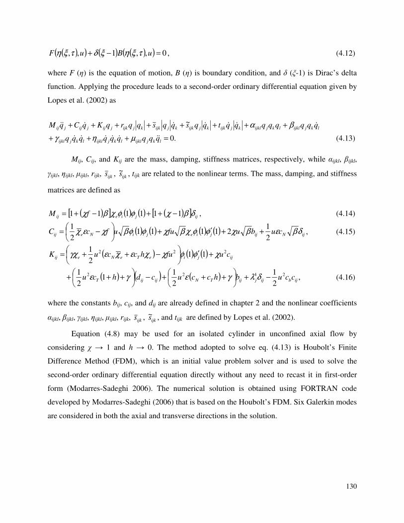
130
( )( ) ( ) ( )( ) 0,,1,, =−+ uBuF τξηξδτξη , (4.12)
where F (η) is the equation of motion, B (η) is boundary condition, and δ (ξ-1) is Dirac’s delta
function. Applying the procedure leads to a second-order ordinary differential equation given by
Lopes et al. (2002) as
lkjijkllkjijklkjijkkjijkkjijkkjijkjijjijjij qqqqqqqqtqqsqqsqqrqKqCqM &&&&&&&& βα ++++++++ ~
.0=+++ lkjijkllkjijkllkjijkl qqqqqqqqq &&&&&&& µηγ (4.13)
Mij, Cij, and Kij are the mass, damping, stiffness matrices, respectively, while αijkl, βijkl,
γijkl, ηijkl, µijkl, rijk, ijks , ijks~ , tijk are related to the nonlinear terms. The mass, damping, and stiffness
matrices are defined as
( )[ ] ( ) ( ) ( )[ ] ijjieij fM δβχφφχβχ 111111 −++−+= , (4.14)
( ) ( ) ( ) ( ) ijNijjiejiNeij cubufuufcC δβεβχφφχβχφφβχεχ2
121111
2
1++′+
−= , (4.15)
( ) ( ) ( ) ijjieTeNeij cufuhccuK 222 112
1χφφχχεχεγχ +′
−++=
( ) ( ) ( ) ,2
1
2
11
2
1 2422
ijbijjijTNijijT ccubhccucdhcu −+
+++−
+++ δλγεγε (4.16)
where the constants bij, cij, and dij are already defined in chapter 2 and the nonlinear coefficients
αijkl, βijkl, γijkl, ηijkl, µijkl, rijk, ijks , ijks~ , and tijk are defined by Lopes et al. (2002).
Equation (4.8) may be used for an isolated cylinder in unconfined axial flow by
considering χ → 1 and h → 0. The method adopted to solve eq. (4.13) is Houbolt’s Finite
Difference Method (FDM), which is an initial value problem solver and is used to solve the
second-order ordinary differential equation directly without any need to recast it in first-order
form (Modarres-Sadeghi 2006). The numerical solution is obtained using FORTRAN code
developed by Modarres-Sadeghi (2006) that is based on the Houbolt’s FDM. Six Galerkin modes
are considered in both the axial and transverse directions in the solution.
131
4.6. Model in Water Flow with Previously Used Force Coefficients
4.6.1. Adequacy of the Nonlinear Solution
Adequacy of the nonlinear solution is established by solving the nonlinear equation especially
for this purpose and comparing the critical flow velocity for the onset of first mode divergence,
ucr,d1, with that obtained by Semler et al. (2002). The solution of the nonlinear equation yields
ucr,d1 = 2.18. The value of ucr,d1 obtained by Semler et al. (2002) is 2.10. The difference is 3.8%,
which may be considered acceptable. Complete comparison is presented in Section 4.8.
4.6.2. Results
First, the results obtained with the force coefficients and other dimensionless parameters
implemented in the nonlinear equation of motion, previously used by Semler et al. (2002), are
presented. These are β = 0.47, f = 0.7, cN = 0.0244, cT = 0.0244, cb = 0.3, cd1 = 0.0, χ = 1, and ε ≈
20.47. The results are obtained in the dimensionless flow velocity range of 0 ≤ u ≤ 8.0. It is
known that for linear theory to be applicable for post-divergence dynamics, the motion must be
small in the vicinity of the equilibrium state. No such condition is required for nonlinear theory.
Therefore, nonlinear theory unconditionally gives reasonably accurate dynamical behaviour of
the system. Figure 4.1 illustrates the typical bifurcation diagram of the generalized coordinate, q1
versus the dimensionless flow velocity, u. The critical flow velocity for the onset of static
instability, i.e., divergence, with the help of the parameters such as the generalized coordinates
and dimensionless displacements describing the state of the system sometimes is difficult to
identify precisely. The reason is that the divergence does not occur abruptly but evolves
gradually from the equilibrium state of the system. But in this case, looking at Fig. 4.1, it seems
to be very clear. The value of q1 remains essentially zero until at ucr,d1 = 2.18, it becomes non-
zero, i.e., a pitchfork bifurcation occurs and the system loses stability by divergence in first
mode; q1 then increases with u. For u ≈ 3.2, q1 begins to decrease, reaches zero, and then
becomes negative over a small range of u. Before q1 crosses the horizontal axis, the mode shape
of the system is transformed from first mode shape to second mode at ucr,d2 ≈ 4.4. This value is
approximate since the transformation is not abrupt but gradual and it is very difficult to precisely
1 Semler et al. (2002) used the symbol cd to represent zero-flow normal coefficient. In the present work,
the same parameter is represented by the symbol c, as also indicated in Chapter 3.
132
locate the critical velocity. The negative q1 indicates that the second mode shape is enhanced to
the extent that q1 crosses the equilibrium position, i.e., the horizontal axis. Subsequently, at ur2 =
5.41, the system is re-stabilized over a short range of u. At ucr,fl2 = 5.55, the solution loses
stability again through a Hopf bifurcation, which results in flutter in the second mode. At higher
flow velocity, the solution shows in first increasing and then decreasing q1. There might be some
unstable solutions beyond ucr,fl2, but the FDM code only gives stable solutions.
The results are obtained using 100,000 sample points in 100 dimensionless time units, τ.
Figure 4.2 shows the time history and phase-plane plot of the system at u = 1.9. Both figures are
obtained by plotting q1 and q1 against τ ≤ 16 since a stable solution is obtained even before this
time and there is no need to extend it up to τ = 100. Both plots clearly demonstrate a stable
system; the system returning to equilibrium position after initial perturbation. Figure 4.3 shows
the time history, phase-plane plot, and the mode shape at u = 2.6. All three plots clearly
demonstrate that the system has undergone a static instability, i.e., divergence. The saddle point
is shifted to a new location. Figure 4.4 demonstrate second-mode shape divergence of the system
at u = 5.0 with the help of time history, phase-plane plot, and mode shape. The dynamically
unstable system in second mode flutter is shown in Fig. 4.5 at u = 6.3 with the help of time
history, Fast Fourier Transform (FFT), Power Spectral Density (PSD), phase-plane plot,
Poincaré map, and the mode shape. The phase-plane plot is obtained by plotting q1 versus q1; q1
is the derivative of q1 with respect to the dimensionless time τ. The Poincaré map is obtained by
plotting q1 versus q1 whenever the time derivative of second generalized coordinate, q2 = 0. The
system oscillates around the original equilibrium position demonstrating periodic response. This
is confirmed by the phase-plane plot showing, eventually, a stable limit cycle and the Poincaré
map showing all the data points located at only two positions. It means that whenever the
condition of q2 = 0 is met, q1 is located at the same positions in the upper and lower halves of the
periodic oscillation cycles with the same corresponding q1 in one or the other direction. The
negative and positive values of q1 and q1 are based on the sign convention for differentiation.
The initial transient response is omitted in the Poincaré map. The flutter frequency, ffl2, is 1.89
Hz. 3ffl2 is a multiple of the fundamental frequency as shown by PSD in Fig. 4.5 (c).
133
4.7. Model in Water Flow with Presently Calculated Force Coefficients
4.7.1. Adequacy of the Nonlinear Solution
Adequacy of the nonlinear solution with the presently calculated force coefficients is established
by solving the nonlinear equation especially for this purpose and comparing the critical flow
velocity for the onset of first mode divergence, ucr,d1, with the experimental one. The solution of
the nonlinear equation yields ucr,d1 = 1.89. The measured critical flow velocity, ucr,d1, in
experiments is 1.87 (Chapter 2). The difference is 1.07%, which is in good agreement.
4.7.2. Results
The force coefficients, calculated in Chapter 3, are going to be used in the nonlinear model
instead of the previously used ones by Semler et al. (2002) since these are calculated based on
the parameters of the cantilevered cylinder case under investigation and represent more precisely
the fluid forces acting on the cylindrical system. The results thus obtained with these presently
calculated force coefficients are presented in this section. To remind the reader, these force
coefficients are longitudinal viscous coefficient, cT = 0.0234 [cT = 0.0244], normal viscous
coefficient, cN = 0.0041 [cN = 0.0244], base drag coefficient, cb = 0.2024 [cb = 0.3], and zero
flow normal coefficient, c = 0.0510 [cd = 0.0], with the coefficients used previously by Semler et
al. (2002) shown in square brackets. Other parameters are β = 0.5, f = 0.8, γ = 1.23, and χ = 1.
The dimensionless cylinder length, ε is equal to 20.7283. The results are obtained for the
dimensionless flow velocity range of 0 ≤ u ≤ 7.2. Six Galerkin modes are used in the solution. In
this case too, the first bifurcation is clear and the onset of first point of instability can be obtained
without much difficulty, as can be seen in Fig. 4.6, which illustrates the typical bifurcation
diagram of the generalized coordinate, q1 against the dimensionless flow velocity, u. The system
first losses stability by first mode divergence via pitchfork bifurcation at ucr,d1 = 1.89. This is
shown by the increase in q1. With increasing flow velocity, the plot shows an ascend in q1. Later,
q1 start to descend at u = 2.9 and eventually crosses the equilibrium position and becomes
negative at 4.76 < u < 4.77. Before this happens, the first mode divergence transforms gradually
into second mode at ucr,d2 ≈ 4.4. The system again returns to equilibrium state at ur2 = 5.25. This
is indicated by q1 becoming zero. The system remains stable over a short range of u and then
becomes dynamically unstable by coupled-mode flutter at ucr,fl1,2 = 5.29. This coupled-mode
134
flutter involves first and second cylinder modes and is observed in the forthcoming results. At u
> 7.2, unstable solutions also co-exist and the dynamics of the system becomes more intricate.
These results also are obtained using 100,000 sample points in 100 dimensionless time
units, τ. Figure 4.7 shows the time history and phase-plane plot of the system at u = 1.8. Both
figures are obtained by plotting q1 and q1 against τ ≤ 16 since a stable solution is obtained even
before this time and there is no need to extend it up to τ = 100. Both plots clearly demonstrate a
stable system; the system returning to equilibrium position after initial perturbation. Figure 4.8
shows the diverged system in first mode with the help of time history, phase-plane plot, and the
mode shape at u = 2.6. Figure 4.9 shows the diverged system in second mode at u = 5.1. In Figs
4.8 (b) and 4.9 (b), q1 moves to new fixed points, i.e., saddle points. Dynamic instability of the
system is shown with the help of time history, FFT, PSD, phase-plane plot, Poincaré map, and
the mode shape in Fig. 4.10 at u = 5.8. The flutter frequency at this flow velocity is, ffl1,2 = 1.95
Hz. 3ffl1,2 is the multiple of the fundamental frequency as shown in Fig. 4.10 (c). The phase-plane
plot, as shown in Fig. 4.10 (d), depicts a stable limit cycle. The Poincaré map, as shown in Fig.
4.10 (e), confirms periodic motion of the system. The coalesced first and second modes are
observed in the mode shape of the system presented in Fig. 4.10 (f). It means the cylinder
oscillates in its second mode around a diverged position leading to an asymmetric response.
4.8. Comparison of the Results
The results in terms of critical velocities obtained in present work are compared with those
obtained by Semler et al. (2002) in Table 4.1. The present results are obtained by solving the
nonlinear equation of motion numerically using Houbolt’s FDM, whereas Semler et al. used two
different numerical schemes namely FDM and AUTO. The software AUTO is based on a
collocation method. It is adapted to solving continuation and bifurcation problems for differential
equations. The small difference in the results is due to different numerical schemes used. In other
words, the difference is attributed to numerical error of the schemes. Overall, the agreement is
good.
The models employing previously used and presently calculated force coefficients are
compared in Table 4.2, which shows a salient difference in the post-divergence dynamics
depicting coupled-mode flutter in the model employing the presently calculated force
coefficients, i.e., the system oscillates in second beam mode around first beam mode buckled
135
position. In other words, the first and second modes coalesce and leave the axis with finite q1
indicating the onset of coupled-mode flutter. Other observation is that the divergence of the
system with present force coefficients occur at lower ucr,d1 (13.3 % lower) and ucr,fl1,2 (4.68 %
lower) than with previous ones. It can be reasoned by looking at the values of the present force
coefficients and establishing how these affect the dynamics of the system. It is noticed that the
presently calculated force coefficients cT, cN, and cb are smaller, whereas the coefficient c is
bigger than the previous ones. These present values affect the system by reducing its damping
and stiffness through eqs. (4.15) and (4.16). The eventual result is that the system diverges in
first mode and oscillates in second mode at relatively lower critical flow velocities, ucr,d1 and
ucr,f1,2, respectively. The results of the nonlinear model with the presently calculated force
coefficients demonstrate similar dynamics as observed in the experiments, especially the
combined first mode divergence and second mode flutter as the coupled-mode flutter (such type
of flutter leads to an asymmetric response, as shown in Fig. 4.10(f) and also observed in Figs.
2.32 and 2.33 in Chapter 2). Hence, it can be inferred that the nonlinear model with the presently
calculated force coefficients predicts the dynamics of the system better than the one with the
previously used force coefficients.
4.9. Summary
In this chapter, the nonlinear equation of motion, governing the dynamics of cantilevered
cylinder and derived by Lopes et al. (2002), was solved numerically using Finite Difference
method (FDM). Six Galerkin modes were used for the solution. The downstream free end of the
cylinder was terminated by an ogival end-piece. Two cases were studied; one with the previously
used force coefficients and the other with the presently calculated ones. Results were obtained
for a velocity range of 0 ≤ u ≤ 8.0 and 0 ≤ u ≤ 7.2 for the cases with previous and present force
coefficients, respectively.
The first case showed that the system first lost stability by first mode divergence. At
higher flow velocity, the divergence transformed form first-mode shape to second-mode shape.
As the velocity increased further, the system stabilized by returning to the equilibrium position
for a short range of flow velocity. Then it lost stability by second mode flutter. Results showed
that the flutter exhibited periodic response. The second case (present force coefficients) showed
more or less the same system dynamics with an eminent difference that the post-divergence
136
flutter was in fact of the coupled-mode type, i.e., the combination of first divergence and second
mode flutter. This chapter presented the results in view of the fact established earlier in the work
by Paїdoussis (2004) that nonlinear theory predicts the post-divergence dynamics of the system
more accurately than the linear theory.
Finally, the results obtained by the present work with previously used force coefficients
were compared with those by Semler et al. (2002) and then with the ones using the presently
calculated coefficients. The first comparison showed reasonable agreement.
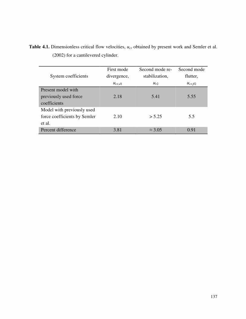
137
Table 4.1. Dimensionless critical flow velocities, ucr obtained by present work and Semler et al.
(2002) for a cantilevered cylinder.
System coefficients
First mode
divergence,
ucr,d1
Second mode re-
stabilization,
ur2
Second mode
flutter,
ucr,fl2
Present model with
previously used force
coefficients
2.18 5.41 5.55
Model with previously used
force coefficients by Semler
et al.
2.10 > 5.25 5.5
Percent difference 3.81 ≈ 3.05 0.91
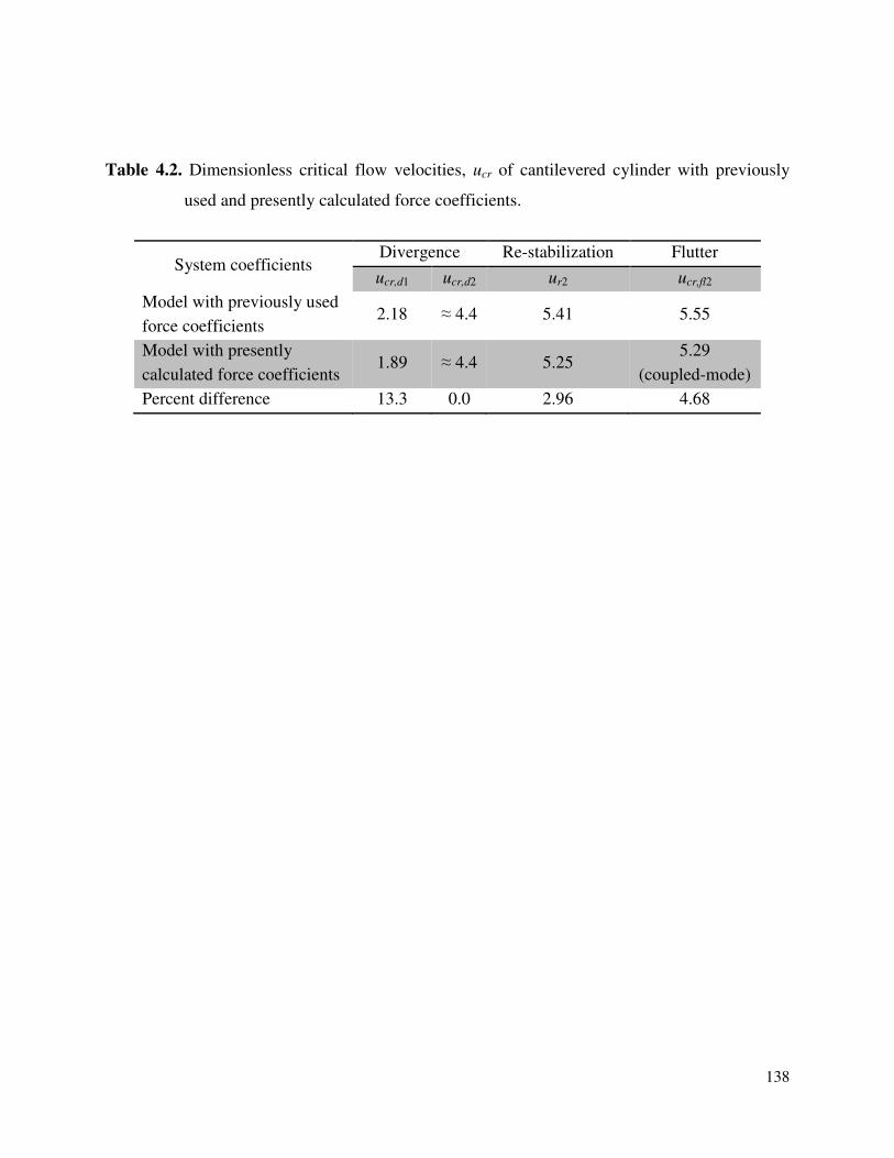
138
Table 4.2. Dimensionless critical flow velocities, ucr of cantilevered cylinder with previously
used and presently calculated force coefficients.
System coefficients Divergence Re-stabilization Flutter
ucr,d1 ucr,d2 ur2 ucr,fl2
Model with previously used
force coefficients 2.18 ≈ 4.4 5.41 5.55
Model with presently
calculated force coefficients 1.89 ≈ 4.4 5.25
5.29
(coupled-mode)
Percent difference 13.3 0.0 2.96 4.68
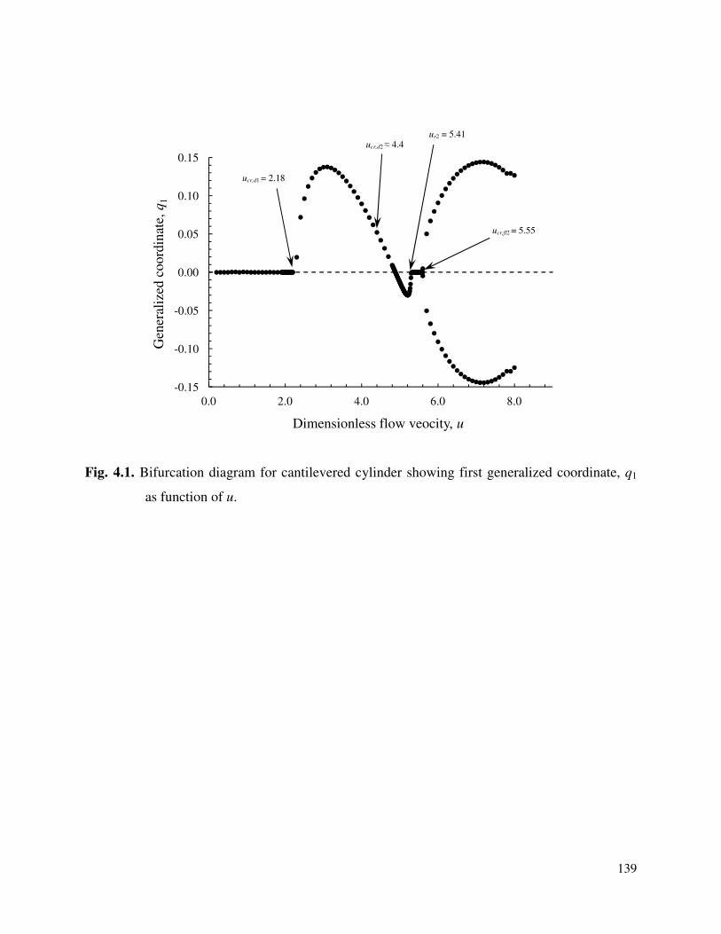
139
Fig. 4.1. Bifurcation diagram for cantilevered cylinder showing first generalized coordinate, q1
as function of u.
-0.15
-0.10
-0.05
0.00
0.05
0.10
0.15
0.0 2.0 4.0 6.0 8.0
Gen
eral
ized
coord
inat
e, q
1
Dimensionless flow veocity, u
ucr,d1 = 2.18
ur2 = 5.41
ucr,fl2 = 5.55
ucr,d2 ≈ 4.4
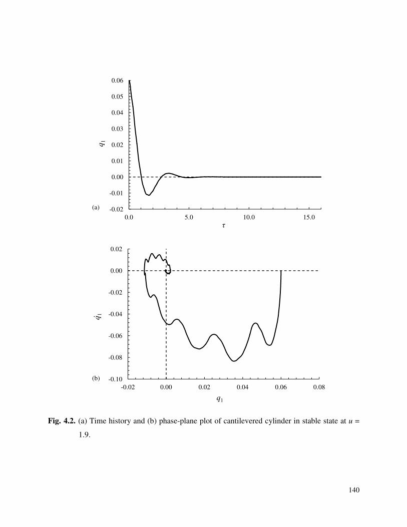
140
Fig. 4.2. (a) Time history and (b) phase-plane plot of cantilevered cylinder in stable state at u =
1.9.
-0.10
-0.08
-0.06
-0.04
-0.02
0.00
0.02
-0.02 0.00 0.02 0.04 0.06 0.08
q1
q1
-0.02
-0.01
0.00
0.01
0.02
0.03
0.04
0.05
0.06
0.0 5.0 10.0 15.0
q1
τ
(a)
(b)
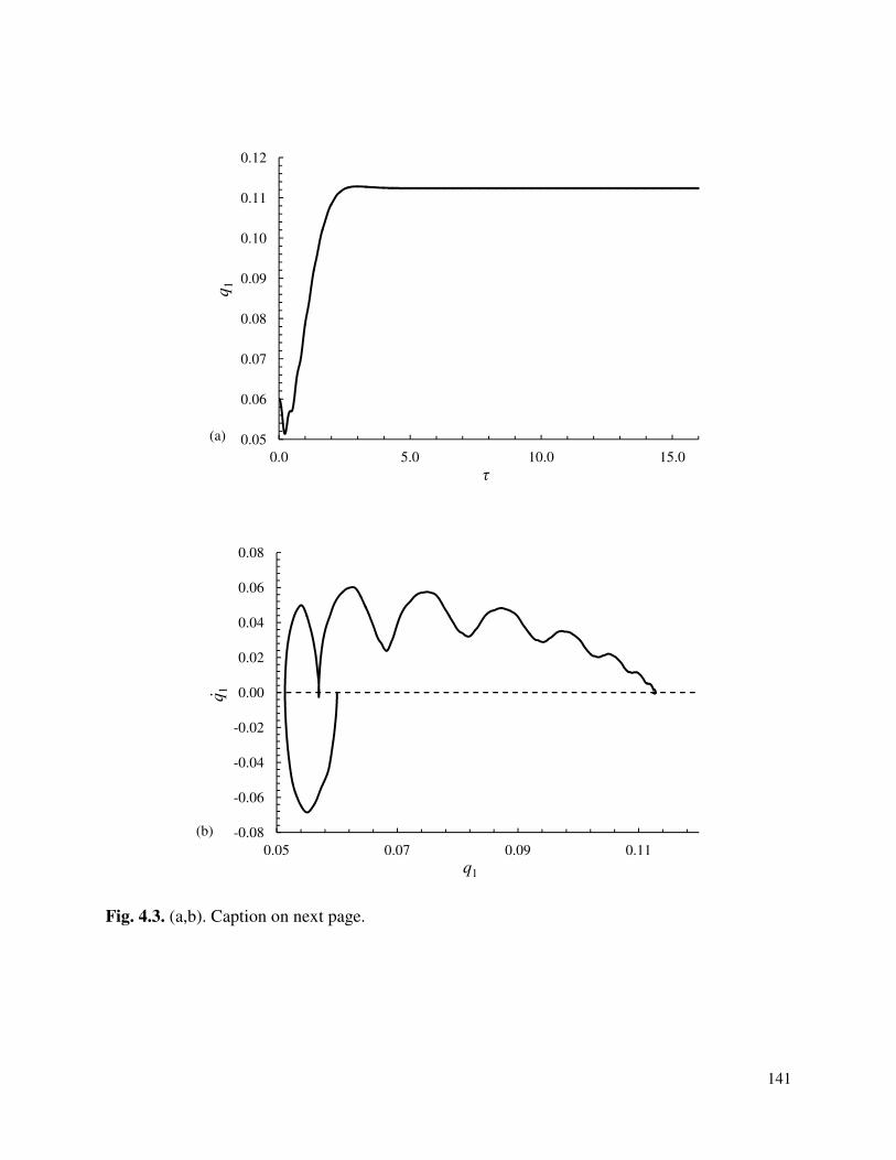
141
Fig. 4.3. (a,b). Caption on next page.
0.05
0.06
0.07
0.08
0.09
0.10
0.11
0.12
0.0 5.0 10.0 15.0
q1
τ
-0.08
-0.06
-0.04
-0.02
0.00
0.02
0.04
0.06
0.08
0.05 0.07 0.09 0.11
q1
q1
(a)
(b)
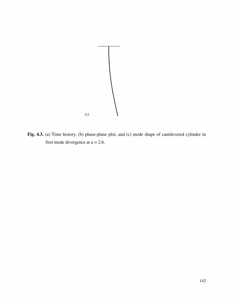
142
Fig. 4.3. (a) Time history, (b) phase-plane plot, and (c) mode shape of cantilevered cylinder in
first mode divergence at u = 2.6.
-3.00E-01 2.00E-01
(c)
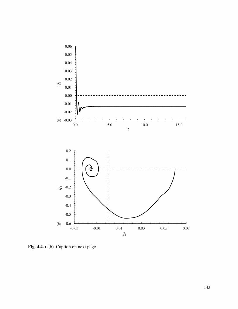
143
Fig. 4.4. (a,b). Caption on next page.
-0.03
-0.02
-0.01
0.00
0.01
0.02
0.03
0.04
0.05
0.06
0.0 5.0 10.0 15.0
q1
τ
-0.6
-0.5
-0.4
-0.3
-0.2
-0.1
0.0
0.1
0.2
-0.03 -0.01 0.01 0.03 0.05 0.07
q1
q1
(a)
(b)
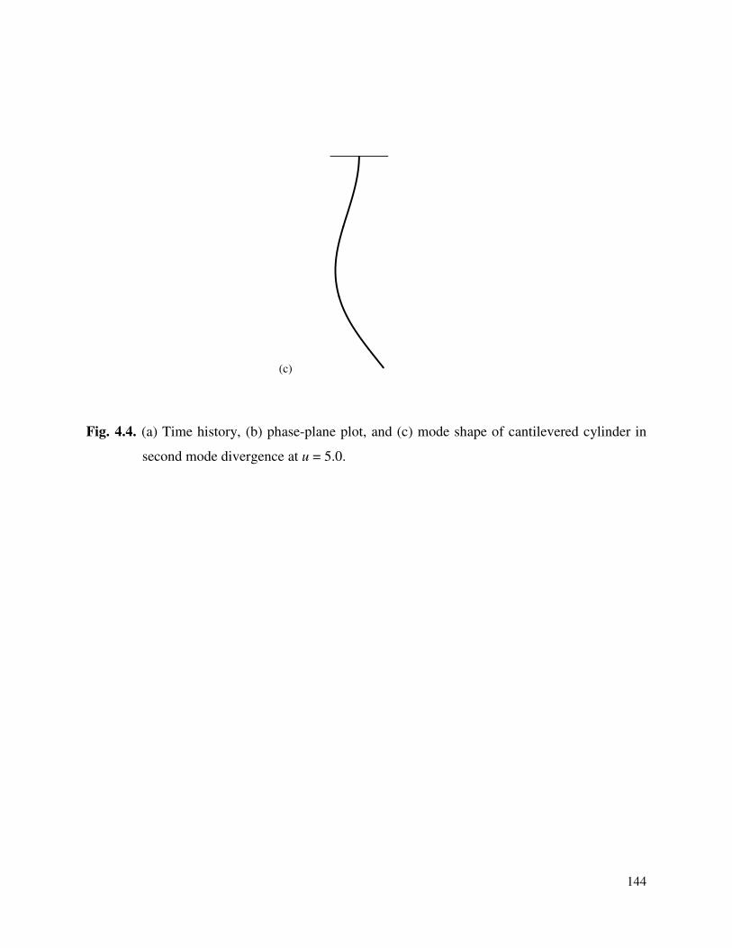
144
Fig. 4.4. (a) Time history, (b) phase-plane plot, and (c) mode shape of cantilevered cylinder in
second mode divergence at u = 5.0.
-8.00E-022.00E-02
(c)
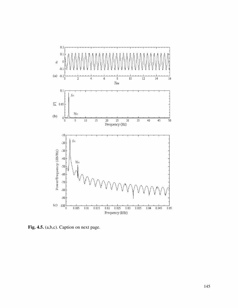
Fig. 4.5. (a,b,c). Caption on next page.
(b)
(a)
(c)
ffl2
3ffl2
ffl2
3ffl2
b,c). Caption on next page.
145
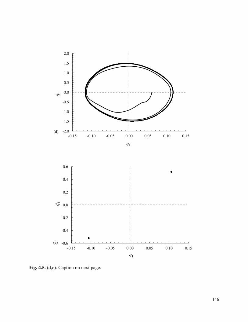
146
Fig. 4.5. (d,e). Caption on next page.
-0.6
-0.4
-0.2
0.0
0.2
0.4
0.6
-0.15 -0.10 -0.05 0.00 0.05 0.10 0.15
q1
q1
-2.0
-1.5
-1.0
-0.5
0.0
0.5
1.0
1.5
2.0
-0.15 -0.10 -0.05 0.00 0.05 0.10 0.15
q1
q1
(d)
(e)
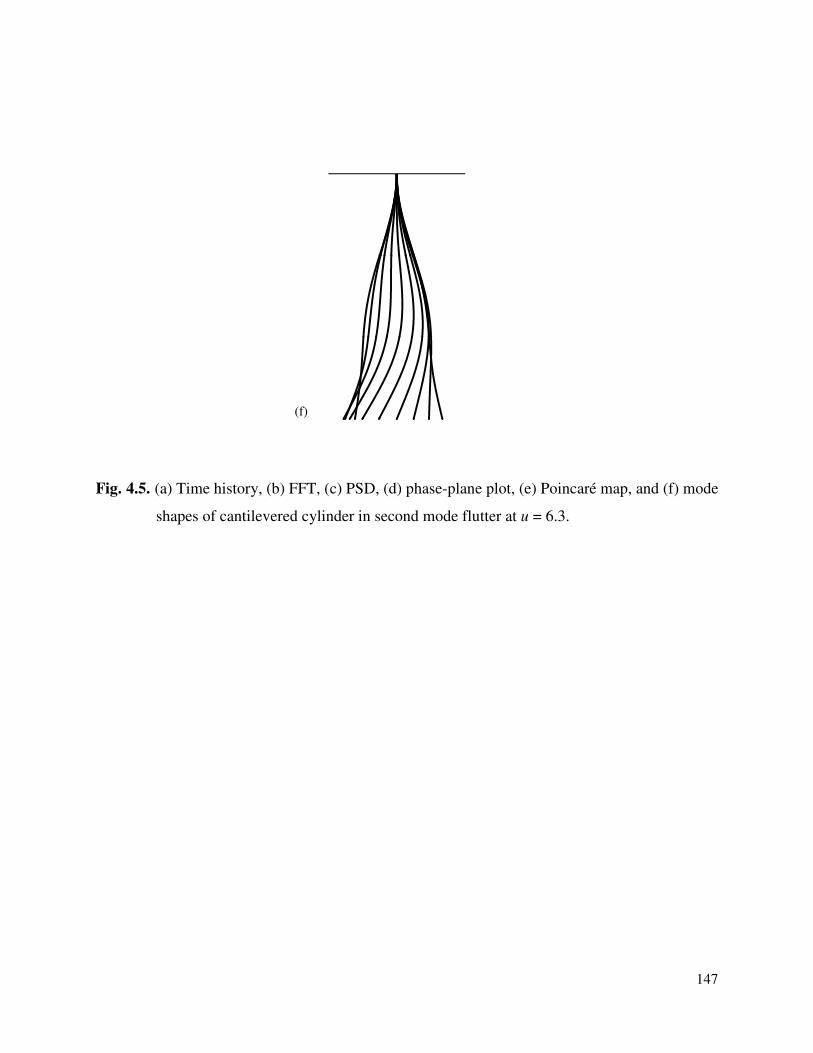
147
-3.00E-01 2.00E-01
Fig. 4.5. (a) Time history, (b) FFT, (c) PSD, (d) phase-plane plot, (e) Poincaré map, and (f) mode
shapes of cantilevered cylinder in second mode flutter at u = 6.3.
(f)
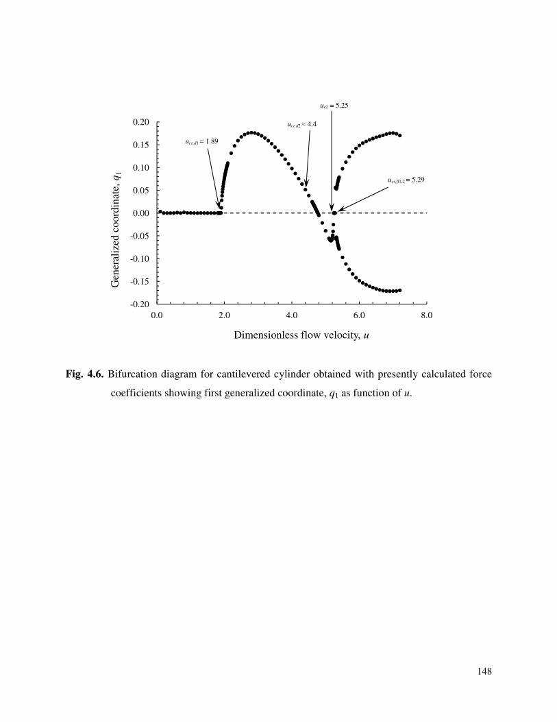
148
Fig. 4.6. Bifurcation diagram for cantilevered cylinder obtained with presently calculated force
coefficients showing first generalized coordinate, q1 as function of u.
-0.20
-0.15
-0.10
-0.05
0.00
0.05
0.10
0.15
0.20
0.0 2.0 4.0 6.0 8.0
Gen
eral
ized
coord
inat
e, q
1
Dimensionless flow velocity, u
ucr,d1 = 1.89
ur2 = 5.25
ucr,fl1,2 = 5.29
ucr,d2 ≈ 4.4
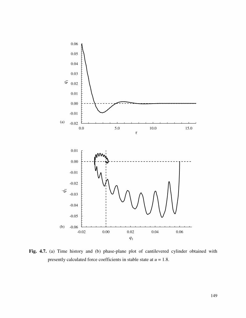
149
Fig. 4.7. (a) Time history and (b) phase-plane plot of cantilevered cylinder obtained with
presently calculated force coefficients in stable state at u = 1.8.
-0.02
-0.01
0.00
0.01
0.02
0.03
0.04
0.05
0.06
0.0 5.0 10.0 15.0
q1
τ
-0.06
-0.05
-0.04
-0.03
-0.02
-0.01
0.00
0.01
-0.02 0.00 0.02 0.04 0.06
q1
q1
(b)
(a)
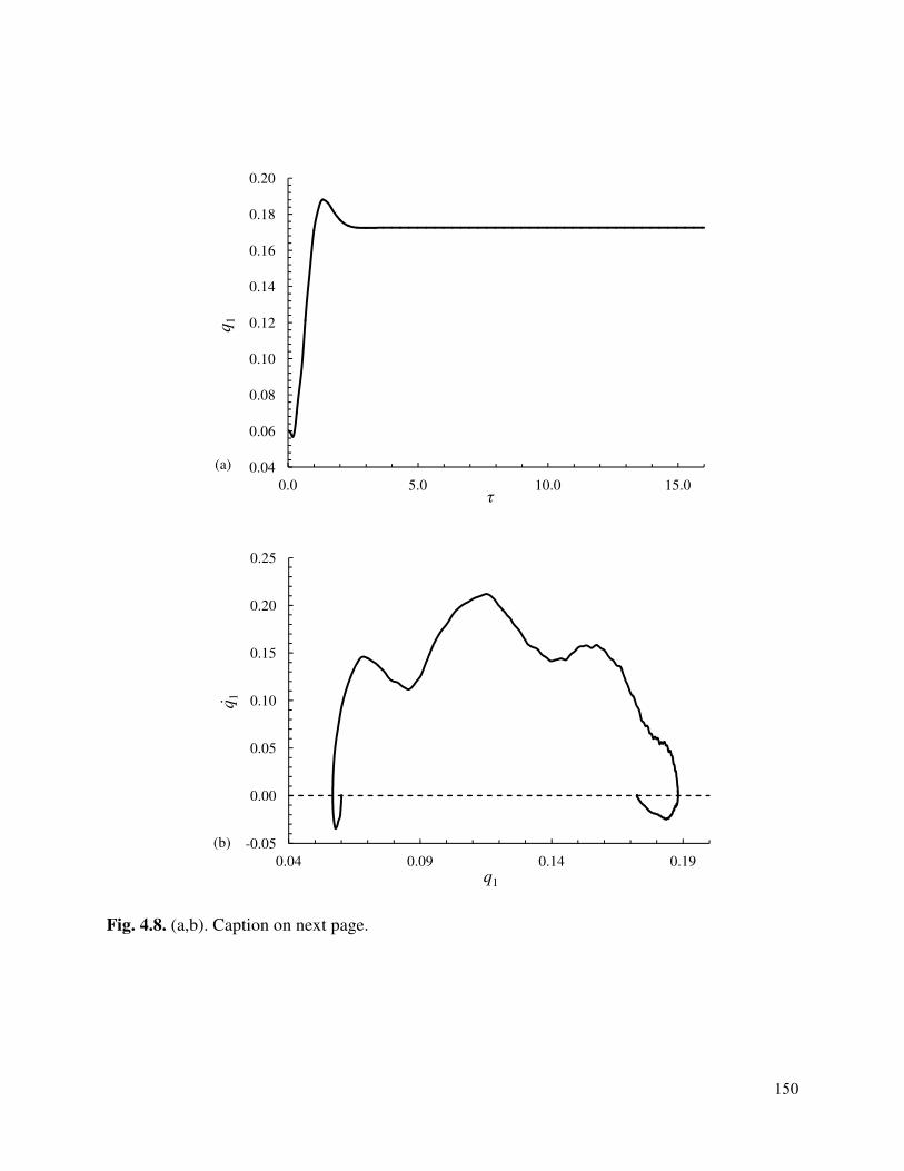
150
Fig. 4.8. (a,b). Caption on next page.
0.04
0.06
0.08
0.10
0.12
0.14
0.16
0.18
0.20
0.0 5.0 10.0 15.0
q1
τ
(a)
-0.05
0.00
0.05
0.10
0.15
0.20
0.25
0.04 0.09 0.14 0.19q1
q1
(b)
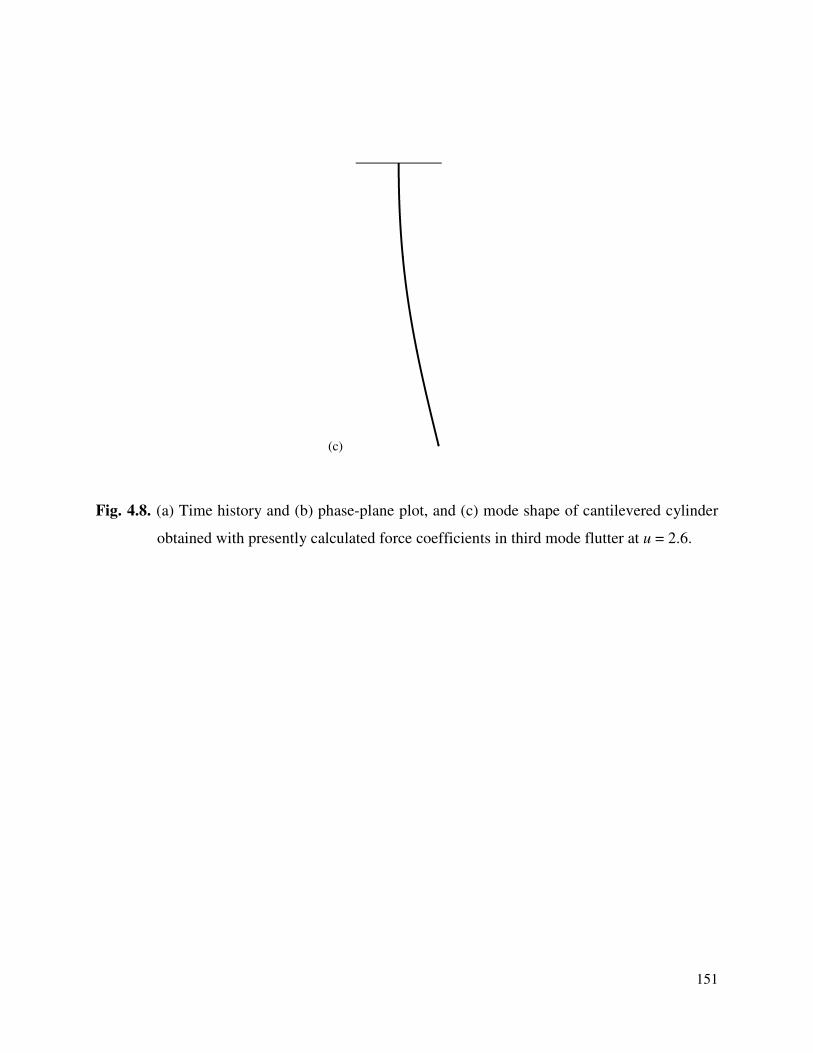
151
Fig. 4.8. (a) Time history and (b) phase-plane plot, and (c) mode shape of cantilevered cylinder
obtained with presently calculated force coefficients in third mode flutter at u = 2.6.
-4.50E-015.00E-02
(c)
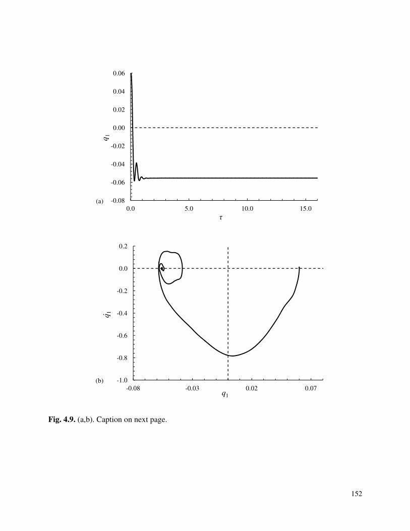
152
Fig. 4.9. (a,b). Caption on next page.
-0.08
-0.06
-0.04
-0.02
0.00
0.02
0.04
0.06
0.0 5.0 10.0 15.0
q1
τ
-1.0
-0.8
-0.6
-0.4
-0.2
0.0
0.2
-0.08 -0.03 0.02 0.07q1
q1
(a)
(b)
153
-1.20E-01 8.00E-02
Fig. 4.9. (a) Time history, (b) phase-plane plot, and (c) mode shape of cantilevered cylinder
obtained with presently calculated force coefficients in third mode flutter at u = 5.1.
(c)
Fig. 4.10. (a,b,c). Caption on next page.
(a)
(b)
(c)
ffl1,2
3ffl1,2
ffl1,2
3ffl1,2
(a,b,c). Caption on next page.
154
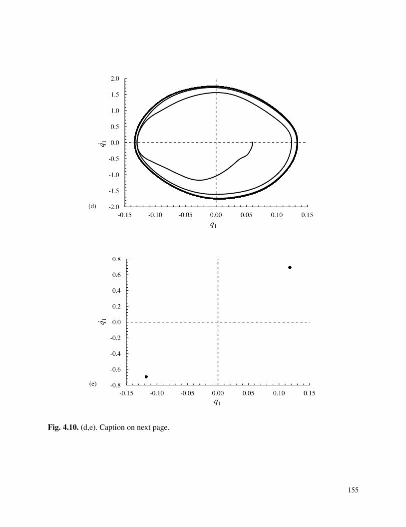
155
Fig. 4.10. (d,e). Caption on next page.
-2.0
-1.5
-1.0
-0.5
0.0
0.5
1.0
1.5
2.0
-0.15 -0.10 -0.05 0.00 0.05 0.10 0.15
q1
q1
(d)
-0.8
-0.6
-0.4
-0.2
0.0
0.2
0.4
0.6
0.8
-0.15 -0.10 -0.05 0.00 0.05 0.10 0.15
q1
q1
(e)
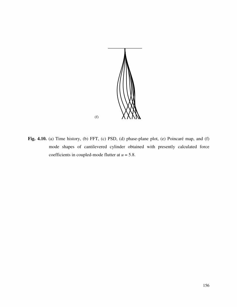
156
Fig. 4.10. (a) Time history, (b) FFT, (c) PSD, (d) phase-plane plot, (e) Poincaré map, and (f)
mode shapes of cantilevered cylinder obtained with presently calculated force
coefficients in coupled-mode flutter at u = 5.8.
-3.00E-01 2.00E-01
(f)
Chapter 5
Numerical Simulations
5.1. Introduction
In all the practical applications and previously conducted experiments relevant to flexible slender
cylindrical structures in axial flow, mentioned in Chapter 1, the dynamical behaviour observed is
three-dimensional. Not only this but the path described by the cylinder end was observed in one
of the experiments (Paїdoussis et al. 2002) to be orbital instead of circular. Lack of knowledge to
account for the three-dimensional behaviour, especially the non-symmetry found in the cylinder
motion, important for the safe operation of the engineering and health delivery processes, is the
motivation behind the present work, which is aimed at developing a three-dimensional coupled
nonlinear model for a confined flexible cylindrical structure in axial flow in an FEM based
modelling and simulation package called ADINA.
In addition to the solutions of the linear and nonlinear equations of motion obtained by
the analytical and numerical techniques, respectively, ADINA is also utilized to solve the
problem under investigation. ADINA is a finite element analysis solver and Simulation software
package for various physics and engineering applications, especially multiphysics or coupled
phenomena such as Fluid-Structure Interaction (FSI). ADINA offers FSI capabilities in one
single program for the solution of problems where the fluids are fully coupled to general
structures that can undergo highly nonlinear response due to large deformations, contact with the
surrounding boundaries, and temperature-dependency. A fully coupled fluid-structure interaction
means that the response of the solid is strongly affected by the response of the fluid, and vice
versa. From the fluid point of view, the Navier-Stokes flow can be incompressible, slightly
compressible, low-speed or high-speed compressible. From the structural point of view, all
available element types can be used (i.e. shell, two-dimensional and three-dimensional solid,
beam, iso-beam, contact surfaces, etc.) as well as all available material models. Once any part of
the computational domain deforms, the Eulerian description of the fluid flow is no longer
applicable. Therefore, ADINA solves the governing equations of fluid flow using an Arbitrary-
Lagrangian-Eulerian (ALE) formulation (ADINA 2012). One of the benefits in developing the
ADINA model is that it gives three-dimensional visualization of the results.
158
5.2. Validation of ADINA
To check the adequacy of ADINA, results from the well known benchmark problems are
compared with the experimental and numerical results obtained previously by other
investigators. If the results obtained from ADINA show good agreement with the previous
results, then it will be considered fit to be used for further analysis. Therefore, the following four
different models were developed: (a) two-dimensional pipe flow model; (b) backward facing step
mode; (c) point load deflection model; (d) three-dimensional point load deflection model.
5.2.1. Two-Dimensional Pipe Flow Model
The validation of ADINA is commenced with a very fundamental fluid mechanics boundary
layer model, i.e., a two-dimensional pipe flow model. Two parameters, the length of the pipe
required to achieve fully developed flow, i.e., the entrance length, and the pressure drop, ∆p
across the pipe of given length. The model of a horizontal pipe of diameter, Dch = 0.05 m is
generated in ADINA. Water enters the pipe from the left at a uniform flow velocity, v = 0.01
m/sec as shown in Fig. 5.1. Standard Temperature and pressure (STP) conditions of water are
considered. The resulting Reynolds number Re, is 500, indicating laminar flow. The flow profile
is checked across the cross-sections of the pipe along its length. The distance from the pipe
entrance at which a fully developed parabolic flow profile is obtained is marked as the entrance
length, Lent. The resulting dimensionless value, Lent/Dch, comes out to be 29.8. Then, the standard
relation for the entrance length in laminar pipe flow is considered (Shaughnessy et al. 2005)
Re06.0=ch
ent
D
L. (5.1)
For a Re of 500, the dimensionless entrance length, Lent/Dch, is 30. The difference between the
ADINA and theoretical result is 0.67 %.
In order to determine the pressure drop, ∆p, in a two-dimensional pipe of given length, a
similar model with the same flow parameters as used for the entrance length is considered in
ADINA. The length of the pipe Lch is prescribed as 1 m. Simulation of the model in ADINA
gives ∆p of 0.126 Pa. The standard relation of pressure drop across a pipe is given by
(Shaughnessy et al. 2005)
159
2
221 k
ch
chD
v
D
Lf
pp=
−
ρ (5.2)
or
,2
2k
ch
chD
v
D
Lfp
ρ=∆ (5.3)
where fD is the Darcy-Weisbach friction coefficient. For laminar flow, it is equal to 64/Re. For a
flow velocity of 0.01 m/s, the theoretical value of ∆p obtained from eq. (5.3) is equal to 0.128
Pa. The difference between ADINA and theoretical values is 1.56 %.
5.2.2. Backward Facing Step Model
The validity of ADINA is further verified by comparing the results for backward facing step in a
rectangular duct model with the experimental and numerical results. The model developed in
ADINA is shown in Fig. 5.2. Flow enters the inlet from left. Flow separation occurs right after
the flow passes over the backward facing step of height sh. It reattaches to the duct bottom wall
after a certain distance x. Therefore, the parameter selected for comparison is the reattachment
length x of the fluid flow with the duct wall. Figure 5.3 shows the flow velocity profile
development with the help of velocity vectors and velocity contours on the duct cross-sections
along the length of the duct.
The first comparison is carried out with the results of Nie and Armaly (2003). They
performed numerical simulations for incompressible three-dimensional laminar forced
convection flow adjacent to backward facing step in a rectangular duct in order to examine the
reattachment region of the separated flow on the stepped wall. They selected the dimensions of
the duct in such a way that the flow at the inlet section of the duct (x/sh = -2) was not affected
significantly by the sudden expansion in the geometry at the step, and the flow at the exit section
(x/sh = 50) was fully developed. It was also insured through measurements that the flow was
laminar and steady for Reynolds number less than 600. Considering Re = 400, they obtained the
dimensionless reattachment length, x/sh = 7.6. Similar initial and boundary condition have been
adopted in the ADINA model. The dimensionless reattachment length, x/sh thus obtained is 7.5.
The difference is 1.32 %.
160
The other comparison is with the experimental result of the same parameter, i.e., flow
reattachment length, obtained by Williams and Baker (1996). They considered a three-
dimensional backward facing step model and ran numerical simulations at different Reynolds
number, Re to compare with the work of Armaly et al. (1983). For Re = 800, they obtained the
dimensionless reattachment length, x/sh = 14. Simulating the same model in ADINA gives value
of x/sh = 13.122. The difference is 6.27 %.
5.2.3. Point Load Deflection Model
ADINA has also been tested for the purely structural mechanics part. A two-dimensional
horizontal beam model of length, lbeam = 1 m, height, b = 0.02, infinite width, subjected to a
vertical concentrated point load, W = 1 N at the tip of the beam is generated in ADINA as shown
in Fig. 5.4. The beam material is steel with modulus of elasticity, E = 2.07×10¹¹
Pa and second
moment of area, I = 1.33×10⁻⁸
m4. The beam tip deflects 1.20773×10
-4 m downwards. Increasing
the point load to 300 N results in a tip deflection of 3.623×10⁻²
m. The relation of maximum
beam deflection under a concentrated point load at the tip is given by (Ryder 1969)
.3
3
maxEI
Wlbeam−=δ (5.4)
The negative sign signifies downward deflection, in negative y-direction. Substituting the
parameters of the ADINA beam model, values of δmax = 1.21×10⁻⁴
m and 3.632×10⁻²
m for point
loads of 1 N and 300 N, respectively, are obtained. The corresponding differences between
theory and ADINA are 0.19 % and 0.25 %, respectively.
5.2.4. Three-Dimensional Point Load Deflection Model
A horizontal circular flexible silicone rubber of cylinder length, l = 0.483 m, diameter, D =
0.0254 m, modulus of elasticity, E = 2.76×10⁶ Pa, and second moment of area, I = 2.0435×10
-8
m4 subjected to a vertical concentrated tip load, W = 0.1 N, in the negative y-direction is
considered. The model generated in ADINA is shown in Fig. 5.5. The maximum deflection of
the cylinder end, δmax, thus obtained is 6.61×10⁻²
m. Making use of eq. (5.4) and substituting in
the same parameters, δmax thus obtained is 6.66×10⁻²
m. The discrepancy between theory and
ADINA is 0.75 %.
161
The good agreement displayed in the above validation tests between ADINA and
analytical results have built up confidence that the ADINA model can safely be used to develop,
simulate, and analyze the FSI model of the problem under consideration in this thesis.
5.3. Model Description
The three-dimensional FSI flexible cantilevered cylinder model is generated in ADINA in its two
modules namely ADINA CFD and ADINA Structures. Dealing first with the fluid part of the
model in ADINA CFD, a circular channel of diameter, Dch = 0.203 m and length, Lch = 0.77 m is
generated. Then the outlines of the cylinder and the upstream supports are generated. The
cylinder outline serves as an FSI boundary across which the information of fluid forces and solid
motion/deformation is passed and the support outline serves as rigid wall. The fluid domain of
the FSI model is first descritized. This is done by dividing the surfaces of the fluid domain into
segments ranging from 10 to 60, resulting in a mesh density of around 5.6×10⁶ elements/m
3. An
unstructured mesh is then generated by the option available in the software. This creates the
meshed fluid domain as shown in Fig. 5.6 (a). For model’s solid part in ADINA Structures, the
cylinder and the upstream support are generated in such a way that the physical surfaces of these
structures match the surfaces of the same in the model’s fluid part. In a similar way, the cylinder
surface is set as the FSI boundary whereas the support as a rigid wall. This matching consistency
ensures two-way continuity of information flow across the boundaries and helps ADINA to
develop coupling between the fluid and solid domains. The cylinder material is silicone rubber,
with modulus of elasticity, E = 2.76×10⁶ Pa, flexural rigidity, EI = 5.6391×10
-2 N m
2, density, ρ
= 1120 kg/m3, diameter, D = 0.0254 m, and length, L = 0.52 m. The cylinder is terminated by a
conical end-piece of length, l = 0.037 m and end-shape factor, f ≈ 0.48; the procedures to
calculate f is given in Appendix A. The upstream support consists of four perpendicular arms.
These are designed in such a way as to keep the flow past the support as streamlined as possible.
The material of the support is taken as steel with E = 2.0×10¹¹
Pa. The solid domain of the FSI
model is then descritized. This is done by dividing the surfaces of the solid domain into the same
number of segments as the fluid domain surfaces in order to match the nodes on all the common
surfaces of both the domains. The resulting mesh density of solid domain obtained is around
7.8×10⁷ elements/m
3. Similar to fluid domain, an unstructured mesh is generated. The meshed
solid domain is shown in Fig. 5.6 (b). The values of χ (defined in Chapter 2) and α (defined in

162
Chapter 3) for the present model are equal to 1.03 and 7.99, respectively. As indicated earlier,
the value of χ arrow 1 (Chapter 2) and α >> 1 (Chapter 3) indicates the case of an unconfined
flow. Therefore, the present model, as pointed out by the values of χ and α, is essentially the case
of an unconfined flow.
ADINA simulations are carried out for two different fluids, namely water and air.
Different dynamics of the cylinder is obtained for the two fluids. A model without the upstream
support arms is also generated and simulated for velocities beyond the critical velocity for flutter
in water flow and for the entire velocity range in air flow as shown in Fig 5.7. The faces of the
model are divided into segments ranging from 5 to 30 resulting in mesh densities of around
5.2×10⁵ and 7.2×10
6 elements/m
3 in CFD and solid parts, respectively. Such mesh densities also
produce reasonable results. The results of both simulations are presented and compared
hereunder.
5.4. CFL Condition
The Courant–Friedrichs–Lewy (CFL) condition is a necessary condition for convergence while
solving certain partial differential equations numerically. It arises in the numerical analysis of
time-marching schemes, when these are used for the numerical solution. The time step must be
less than a certain time in many time-marching computer simulations; otherwise the simulation
will produce incorrect results. The CFL condition is commonly prescribed for those terms of
the finite-difference approximation of general partial differential equations, which model
the advection phenomenon (Courant et al. 1967). The Courant number, in fact, reflects the
portion of a cell that a fluid particle will traverse by advection in one time step. For a one-
dimensional case, the CFL has the form
,maxCx
tUC ≤
∆
∆= (5.5)
where U is the dimensional flow velocity, ∆t is the time step, ∆x is the length interval, and C is
the Courant number. Cmax is the maximum value of Courant number that helps in determining the
minimum value of time step. The value of Cmax changes with the method used to solve the
discretized equation. If a time-marching solver is used, then typically Cmax = 1. ∆t can be
determined by re-adjusting eq. (5.5) as
163
.U
xCt
∆=∆ (5.6)
Since C = 1, the equation becomes
.U
xt
∆=∆ (5.7)
The simulation has been run for flow velocities up to 6.41 m/s. In order to obtain one
consistent value of ∆t for the entire simulation, a mean value of flow velocity is considered, i.e.,
U = 3.21 m/s; the corresponding dimensionless velocity is u = 5.0. With the unstructured mesh
in both fluid and solid domains, the minimum and maximum length intervals, ∆x, are found to be
0.0039 m and 0.0425 m, respectively. Substituting U and the terminal values of ∆x in eq. (5.7)
gives 0.001 ≤ ∆t ≤ 0.01 s. It is good to have a value of ∆t close to the lower limit especially at the
initial stages of the simulation and cylinder higher frequency modes, because of the conditions
being unsteady and developing, and changes in the parameters taking place mode rapidly. But
limitations are imposed on the use of the value of ∆t smaller than a certain limit. The reason
being that for a three-dimensional model, smaller ∆t increases the simulation time many folds
and makes the size of the output file beyond the capabilities of many powerful systems with
large memories. For this reason, ∆t = 0.01 s is selected.
5.5. Model in Water Flow
5.5.1. Adequacy of the Numerical Solution
Adequacy of the numerical solution is established by simulating the numerical model especially
for this purpose and comparing the critical flow velocity for the onset of first mode divergence,
ucr,d1, with the experimental one. The results of the numerical model yield ucr,d1 = 1.80. The
measured critical flow velocity, ucr,d1, in experiments is 1.87 (Chapter 2). The difference is 3.74
%, which may be considered acceptable.
5.5.2. Numerical Results
First, the flexible cantilevered cylinder model is considered in water flow. The physical
properties of water at Standard Temperature and Pressure (STP) are input in ADINA. A flow
164
velocity range of 0.064 ≤ U ≤ 8.97 m/s is utilized for the simulation runs. The relation used to
render the flow velocity dimensionless is
,
21
ULEI
Au
=
ρ (5.8)
as given by Paїdoussis (2004). Substituting the input parameters simplifies the relation as u =
1.56 U, which gives the corresponding dimensionless velocity range as 0.1 ≤ u ≤ 14.0. Utilizing
the relation for Re gives its range as 1.3×10⁴ ≤ Re ≤ 1.81×10
6. The k-ω turbulence model is used
for water flow.
Figure 5.8 shows the dimensionless mean cylinder tip displacement, η*(1) = ȳ(L)/D, as a
function of u. The figure illustrates the dynamics of the cylinder up to static instability, i.e.,
divergence. It is also clear from the figure that divergence does not develop abruptly. Therefore,
it becomes rather difficult to locate the critical velocity for divergence, precisely. For this reason,
a rougher but reliable criterion of η*(1) surpassing a threshold is used. This threshold is
arbitrarily chosen as η*(1) = 0.023. Physically, this criterion corresponds to about twice the
cylinder diameter. At ucr,d1 = 1.80, η*(1) surpasses the threshold and thus marks the onset of
divergence in its first mode as shown in Fig 5.9 (a). At higher flow velocities, the cylinder
amplitude varies; later, gradually the first mode divergence transforms into second mode at ucr,d2
≈ 4.30 as shown in Fig. 5.9 (b). The second mode divergence is based on visual inspection. The
results are shown in Table 5.1. As the flow velocity increases, one expects the cylinder to
become dynamically unstable with relatively large amplitude oscillations or flutter, which has
been observed previously by Paїdoussis et al. (2002) and Semler et al. (2002) in their analytical
and experimental work at 5.16 ≤ u ≤ 5.5. In fact, reaching the same or even higher values of u
does not produce any flutter in the cylinder in the ADINA simulations, as can be seen in Figs
5.10 (b) and (c). A possible reason might be due to the inherent numerical damping imposed in
ADINA on the solid that damps out the higher mode oscillations.
ADINA employs a conditionally stable algorithm. A conditionally stable algorithm
necessitates that the size of the time step used be inversely proportional to the highest frequency
of the system. In fact, this is a strict limitation, as accuracy in the lower modes can be attained
with time steps which are very large compared with the period of the highest mode. When only
low mode response is of interest, it is often advantageous for an algorithm to have some form of
165
numerical dissipation or damping, which stabilizes the numerical integration scheme by damping
out the unwanted high frequency modes (Hilber et al. 1977). As for ADINA, numerical damping
works well at lower mode static instabilities but introduces a substantial damping effect on the
higher modes, which is not desirable. This inherent unwanted damping effect makes the cylinder
remain in the second mode buckled shape at u ≈ 5.10 as shown in Fig. 5.10 (a); it remains there
for the supposedly post-flutter velocities, u = 5.5 and 5.6 (Figs. 5.10 (b) and (c)). At further
higher dimensionless flow velocity of 8.0, the cylinder develops third mode shape but the
dynamic response is still damped as shown in Fig. 5.10 (d) by the same damping present in the
algorithm. For this velocity and all higher velocities, the upstream support arms are removed in
order to nullify any of their possible effects on the dynamics of the cylinder. A practical way to
reduce its contribution in the overall system damping as much as possible at higher frequency
modes is to decrease the time step. By doing so, the ADINA simulation becomes very expensive
in terms of simulation execution time (it could reach up to a couple of weeks) and size of the
output file (it might reach up to 100 Gigabyte). There are no powerful computing systems at
hand, which can open and post-process the output data of files of such size. For this reason, no
attempt is made to use very small ∆t in the model to handle the numerical damping and obtain
second and third cylinder mode flutter.
In addition to the inherent numerical damping imposed on the system in the software,
it is important to also look into physical aspect such as vortex-induced vibration. Blevins (1990)
explains the underlying physics generating structural vibration subjected to vortex shedding as:
“As a fluid particle flows toward the leading edge of a cylinder, the pressure in the fluid particle
rises from the free stream pressure to the stagnation pressure. The high fluid pressure near the
leading edge impels flow about the cylinder as boundary layers develop about both sides.
However, the high pressure is not sufficient to force the flow about the back of the cylinder at
high Reynolds numbers. Near the widest section of the cylinder, the boundary layers separate
from each side of the cylinder surface and form two shear layers that trail aft in the flow and
bound the wake. Since the innermost portion of the shear layers, which is in contact with the
cylinder, moves much more slowly than the outermost portion of the shear layers, which is in
contact with the free flow, the shear layers roll into the near wake, where they fold on each other
and coalesce into discrete swirling vortices. A regular pattern of vortices, called a vortex street,
trails aft in the wake. The vortices interact with the cylinder and they are the source of the effects
166
called vortex-induced vibration”. Therefore, velocity and pressure contours are obtained at the
cross-sections 0.71 m (7.5 cylinder diameters downstream of cylinder free end) and 0.715 m (7.7
cylinder diameters downstream of cylinder free end) from the channel inlet at dimensionless
turbulent flow velocities u = 5.6 and 8.0, respectively. These contours are shown in Figs. 5.11
and 5.12. Both figures clearly show low velocity and high pressure in the wake region and
relatively high velocity and low pressure in the swirling flow on either sides of the channel
centreline. The apparent swirling flow seems to be part of the vortices. These vortices at the
same cross-sections at both the flow velocities are monitored throughout the simulation but no
vortex shedding advancing with time in either case is detected. This might also be another reason
for the system to have no oscillations because of the absence of vortex shedding. From these
results, a strong need is felt to verify experimentally the presence of vortex shedding in the
present model and to see whether it contributes to the cylinder dynamics.
One of the effective experimental methods to observe the vortex shedding is the particle
Image Velocimetry (PIV). Through PIV, the velocity field across the channel cross-section at
different times can be obtained. It measures the velocity field by taking images shortly after each
other and calculating the distance individual particles travelled within the time intervals. From
the known time difference and the measured displacements, the velocity of each particle is
calculated. This experimental method is beyond the scope of the present investigation and can be
done later as a separate investigation.
5.6. Model in Air Flow
5.6.1. Numerical Results
In addition to the simulations in water flow, the flexible cantilevered cylinder model has also
been considered in air flow. The slender cylinder subjected to air flow is the limiting case of a
practical application of a long train with the last carriage having a tapered end inside a tunnel.
The physical properties of air at Standard Temperature and Pressure (STP) are input in ADINA.
A velcity range of 5 ≤ U ≤ 65 m/s is utilized for the simulations. Substitution of the input
parameters in eq. (5.8) yields u = 0.054 U, so that the corresponding dimensionless velocity
range as 0.27 ≤ u ≤ 3.51. Utilizing the expression for Re gives its range 6.715×10⁴ ≤ Re ≤
8.73×10⁵. The k-ω turbulence model is used for air flow. It is noticeable that the dimensional
167
velocity corresponding to a dimensionless value of, say, u = 3.51 for air is far higher than its
counterpart for water. This is because the relation to render the velocity dimensionless involves
the density of fluid, and water is about 1000 times denser than air. The multiplying factor of the
velocity conversion relation in the case of water is 28.9 times larger than of air. As indicated in
Section 5.3, a cantilevered cylinder model without upstream support arms is used for simulation
in air flow. The reason for that is to eliminate any slight possibility of flow disturbance from the
support arms, especially at higher flow velocities at which flutter may possibly occur.
Figure 5.13 shows the dimensionless mean cylinder tip displacement, η*(1), as a function
of u. The figure illustrates the dynamics of the cylinder up to static instability, i.e., divergence.
Similar to the model in water flow, the cylinder tip magnitudes are very small and the onset of
divergence is gradual. Therefore, a threshold is arbitrarily chosen as η*(1) = 0.04. Any
displacement surpassing this value marks the onset of divergence, which is achieved at ucr,d1 =
1.62. Figure 5.14 (a) shows the orthographic and isometric views of the cylinder first mode. At
higher flow velocities, the cylinder amplitude varies and later, gradually, the first mode
divergence evolves into second mode shape at ucr,d2 ≈ 3.02. The diverged second mode of the
cylinder is shown in Fig. 5.14 (b). The same results are also presented in Table 5.2.
The onset of flutter is identified by obtaining the r.m.s. amplitude, η(1)r.m.s., of the
cylinder end-piece tip response and the PSDs of the vibration signal at increasing flow velocities.
Figure 5.15 shows a typical diagram of η(1)r.m.s. versus u, used to locate flutter. The steep rise of
η(1)r.m.s. before ucr,fl2 does not correspond to a stable solution; the oscillations seem to be in
transition phase. Therefore, any of these values cannot be considered for the flutter critical
velocity. A stable solution for the Hopf bifurcation is obtained at ucr,fl2 = 3.20, which leads to
flutter in the second mode. The reduction in amplitude, after a high of 0.0362 D is reached,
reflects gradual changes in modal shape with increasing u. η(1)r.m.s. values are also tabulated in
Table 5.3. Figure 5.16 shows the PSDs of the vibration signal at u = 1.08, 3.08, and 3.20. Figures
5.16 (a) and (b) show PSDs before first mode divergence and after second mode divergence,
respectively, and display no dominant frequency; whereas Fig. 5.16 (c) shows the PSD at the
onset of second mode flutter and displays a dominant frequency, fcr,fl2 = 3.52 Hz. The
corresponding dimensionless value (ωcr,fl2 = 18.96) is obtained from the expression given in
Paїdoussis (2004).

168
5.7. Comparison of the Results
The critical velocities marking the onset of static and dynamic instabilities of the models in water
and air flow are compared in Table 5.4. Third mode flutter for the model in air flow is not
obtained due to the system’s limitations. The word ‘static’ in the case of the water flow model is
included to indicate inability of the software to exhibit oscillations due to the damping effect as
already explained. The numerical model in air flow shows lower ucr,d1, ucr,d2, and ucr,fl2 than their
counterparts for the model in water flow. One of the possible reasons for the lower ucr,d1 for the
numerical model in air flow is the criterion of the threshold value chosen to mark the onset of
divergence, which can vary based on the judgment. For all the models, the second mode
divergence is evolved from the first mode before the onset of flutter. Since ucr,fl2 for the
numerical model in air flow is lower than for the models in water flow, this makes the ucr,d2 for
the numerical model lower too. The reason for the lower ucr,f2 for the numerical model in air flow
is due to the inherent lower viscous damping of air, as also indicated in Chapter 3. It is also
observed in both the numerical models that the cylinder displacement and oscillation magnitudes
for the entire velocity range are minuscule. It seems that the negative damping of the system
somehow does not increase considerably in ADINA resulting in small magnitudes of cylinder
motion. The numerical and analytical model results in terms of the critical flow velocities for the
onset of instabilities for water and air flows are compared in Chapter 6.
5.8. Summary
In this chapter, after the introduction of the numerical simulation software ADINA, it was
validated followed by the determination of CFL condition for numerical stability. The
cantilevered cylinder in axial flow was then modeled in ADINA FSI and simulated to study its
dynamics in water and air flows. Finally, the two models were compared.
The chapter started with the general introduction of ADINA and its solution capabilities
in various multiphysics phenomena. The software was then validated by developing two-
dimensional pipe model, backward facing step model, point load deflection model, and three-
dimensional point load deflection model in ADINA and comparing their results with the
experimental and theoretical results found in the literature. All showed reasonable agreements.
169
CFL condition was also utilized to determine the time step range necessary for numerical
stability.
The problem under consideration, i.e., cantilevered cylinder in axial flow was modeled in
ADINA with the dimensions and input parameters nearly equal to the experimental values. Two
such models one with upstream support arms and finer mesh and the other without the support
arms and coarser mesh were developed with both models having cylinder downstream ends
terminated by end-pieces. The model was first simulated in water flow and the mean
displacements of cylinder tip at increasing velocities were recorded. Unfortunately, the
simulations could show only the static instability, i.e., divergence in first and second modes even
at velocities beyond ucr,fl2 determined by experiments. Possible explanation is given in Section
5.5. The model without support arms was them simulated in air flow. Mean values of cylinder
dimensionless tip displacements and their r.m.s. values plotted against dimensionless flow
velocities, u, helped determining the critical velocities for divergence, ucr,d1 and ucr,d2 and flutter,
ucr,fl2, respectively. Finally, the models in water and air flows were compared for critical flow
velocities and the results revealed that the critical flow velocities for the model in air flow were
lower than the one in water flow.
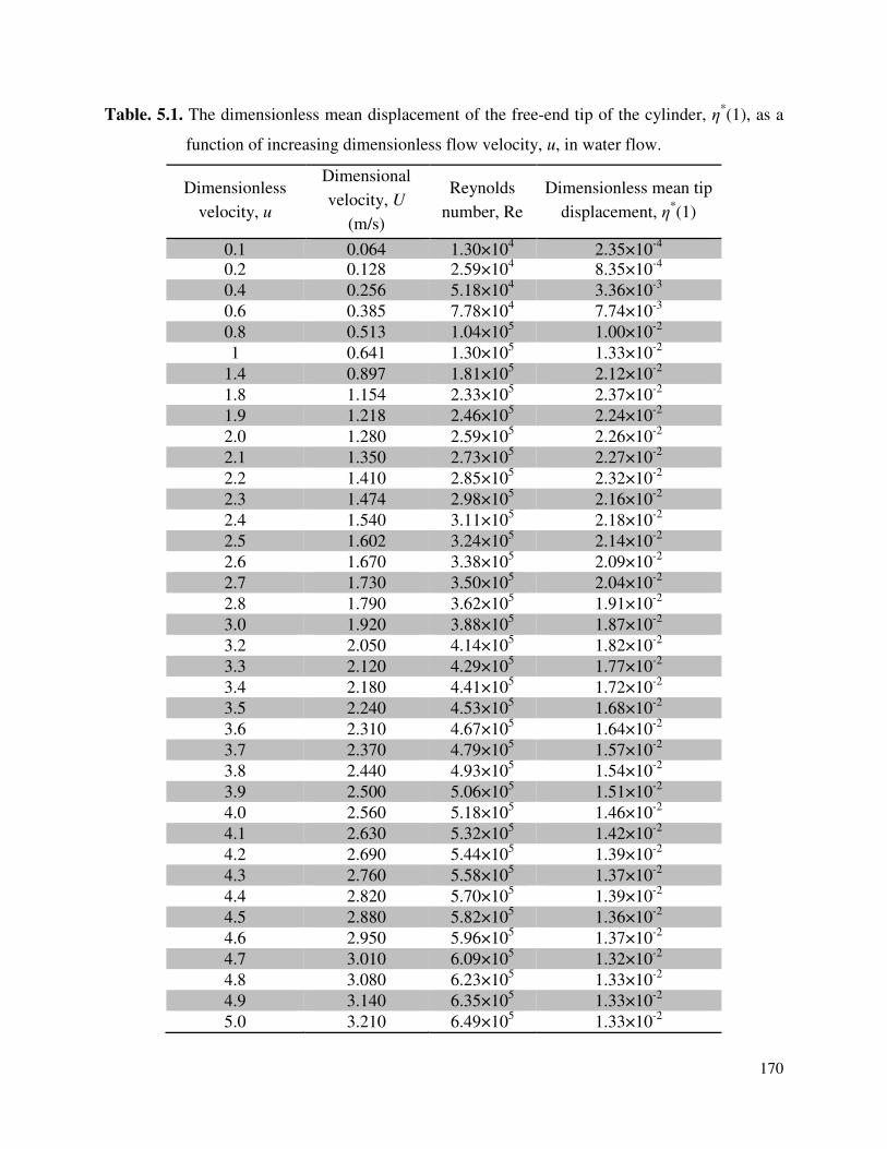
170
Table. 5.1. The dimensionless mean displacement of the free-end tip of the cylinder, η*(1), as a
function of increasing dimensionless flow velocity, u, in water flow.
Dimensionless
velocity, u
Dimensional
velocity, U
(m/s)
Reynolds
number, Re
Dimensionless mean tip
displacement, η*(1)
0.1 0.064 1.30×10⁴ 2.35×10
-4
0.2 0.128 2.59×10⁴ 8.35×10
-4
0.4 0.256 5.18×10⁴ 3.36×10
-3
0.6 0.385 7.78×10⁴ 7.74×10
-3
0.8 0.513 1.04×10⁵ 1.00×10
-2
1 0.641 1.30×10⁵ 1.33×10
-2
1.4 0.897 1.81×10⁵ 2.12×10
-2
1.8 1.154 2.33×10⁵ 2.37×10
-2
1.9 1.218 2.46×10⁵ 2.24×10
-2
2.0 1.280 2.59×10⁵ 2.26×10
-2
2.1 1.350 2.73×10⁵ 2.27×10
-2
2.2 1.410 2.85×10⁵ 2.32×10
-2
2.3 1.474 2.98×10⁵ 2.16×10
-2
2.4 1.540 3.11×10⁵ 2.18×10
-2
2.5 1.602 3.24×10⁵ 2.14×10
-2
2.6 1.670 3.38×10⁵ 2.09×10
-2
2.7 1.730 3.50×10⁵ 2.04×10
-2
2.8 1.790 3.62×10⁵ 1.91×10
-2
3.0 1.920 3.88×10⁵ 1.87×10
-2
3.2 2.050 4.14×10⁵ 1.82×10
-2
3.3 2.120 4.29×10⁵ 1.77×10
-2
3.4 2.180 4.41×10⁵ 1.72×10
-2
3.5 2.240 4.53×10⁵ 1.68×10
-2
3.6 2.310 4.67×10⁵ 1.64×10
-2
3.7 2.370 4.79×10⁵ 1.57×10
-2
3.8 2.440 4.93×10⁵ 1.54×10
-2
3.9 2.500 5.06×10⁵ 1.51×10
-2
4.0 2.560 5.18×10⁵ 1.46×10
-2
4.1 2.630 5.32×10⁵ 1.42×10
-2
4.2 2.690 5.44×10⁵ 1.39×10
-2
4.3 2.760 5.58×10⁵ 1.37×10
-2
4.4 2.820 5.70×10⁵ 1.39×10
-2
4.5 2.880 5.82×10⁵ 1.36×10
-2
4.6 2.950 5.96×10⁵ 1.37×10
-2
4.7 3.010 6.09×10⁵ 1.32×10
-2
4.8 3.080 6.23×10⁵ 1.33×10
-2
4.9 3.140 6.35×10⁵ 1.33×10
-2
5.0 3.210 6.49×10⁵ 1.33×10
-2
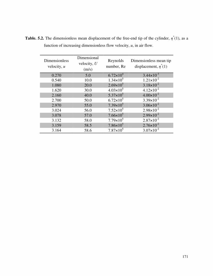
171
Table. 5.2. The dimensionless mean displacement of the free-end tip of the cylinder, η*(1), as a
function of increasing dimensionless flow velocity, u, in air flow.
Dimensionless
velocity, u
Dimensional
velocity, U
(m/s)
Reynolds
number, Re
Dimensionless mean tip
displacement, η*(1)
0.270 5.0 6.72×10⁴ 3.44×10
-3
0.540 10.0 1.34×10⁵ 1.21×10
-2
1.080 20.0 2.69×10⁵ 3.18×10
-2
1.620 30.0 4.03×10⁵ 4.12×10
-2
2.160 40.0 5.37×10⁵ 4.00×10
-2
2.700 50.0 6.72×10⁵ 3.39×10
-2
2.970 55.0 7.39×10⁵ 3.06×10
-2
3.024 56.0 7.52×10⁵ 2.98×10
-2
3.078 57.0 7.66×10⁵ 2.99×10
-2
3.132 58.0 7.79×10⁵ 2.87×10
-2
3.159 58.5 7.86×10⁵ 2.76×10
-2
3.164
58.6 7.87×10
5 3.07×10
-2
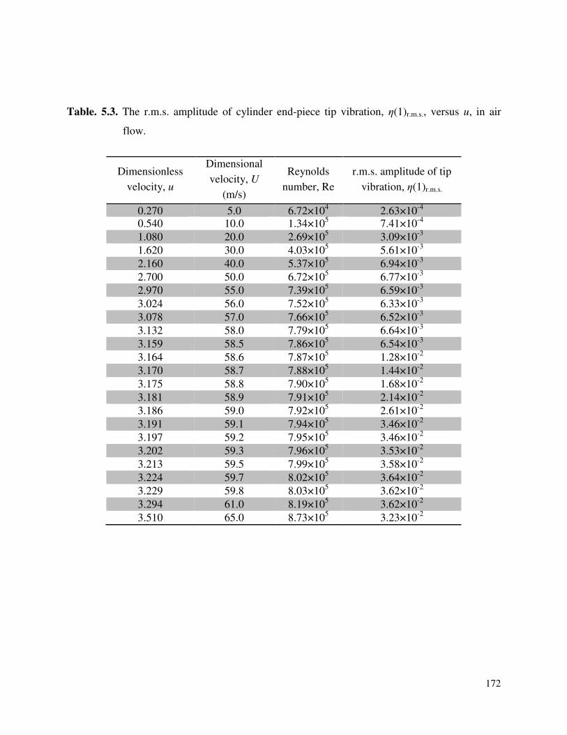
172
Table. 5.3. The r.m.s. amplitude of cylinder end-piece tip vibration, η(1)r.m.s., versus u, in air
flow.
Dimensionless
velocity, u
Dimensional
velocity, U
(m/s)
Reynolds
number, Re
r.m.s. amplitude of tip
vibration, η(1)r.m.s.
0.270 5.0 6.72×10⁴ 2.63×10
-4
0.540 10.0 1.34×10⁵ 7.41×10
-4
1.080 20.0 2.69×10⁵ 3.09×10
-3
1.620 30.0 4.03×10⁵ 5.61×10
-3
2.160 40.0 5.37×10⁵ 6.94×10
-3
2.700 50.0 6.72×10⁵ 6.77×10
-3
2.970 55.0 7.39×10⁵ 6.59×10
-3
3.024 56.0 7.52×10⁵ 6.33×10
-3
3.078 57.0 7.66×10⁵ 6.52×10
-3
3.132 58.0 7.79×10⁵ 6.64×10
-3
3.159 58.5 7.86×10⁵ 6.54×10
-3
3.164 58.6 7.87×10⁵ 1.28×10
-2
3.170 58.7 7.88×10⁵ 1.44×10
-2
3.175 58.8 7.90×10⁵ 1.68×10
-2
3.181 58.9 7.91×10⁵ 2.14×10
-2
3.186 59.0 7.92×10⁵ 2.61×10
-2
3.191 59.1 7.94×10⁵ 3.46×10
-2
3.197 59.2 7.95×10⁵ 3.46×10
-2
3.202 59.3 7.96×10⁵ 3.53×10
-2
3.213 59.5 7.99×10⁵ 3.58×10
-2
3.224 59.7 8.02×10⁵ 3.64×10
-2
3.229 59.8 8.03×10⁵ 3.62×10
-2
3.294 61.0 8.19×10⁵ 3.62×10
-2
3.510 65.0 8.73×10⁵ 3.23×10
-2
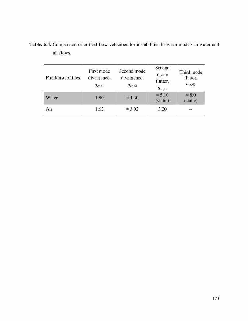
173
Table. 5.4. Comparison of critical flow velocities for instabilities between models in water and
air flows.
Fluid/instabilities
First mode
divergence,
ucr,d1
Second mode
divergence,
ucr,d2
Second
mode
flutter,
ucr,fl2
Third mode
flutter,
ucr,fl3
Water 1.80 ≈ 4.30 ≈ 5.10
(static)
≈ 8.0
(static)
Air 1.62 ≈ 3.02 3.20 --
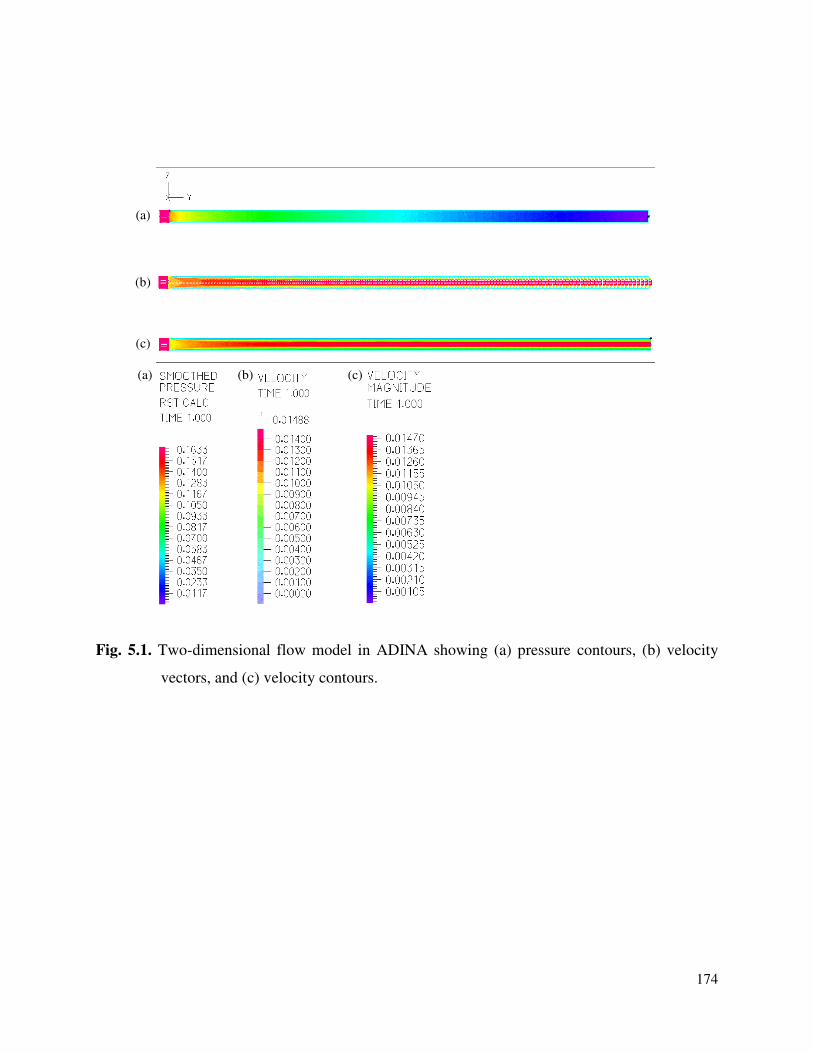
174
Fig. 5.1. Two-dimensional flow model in ADINA showing (a) pressure contours, (b) velocity
vectors, and (c) velocity contours.
(b)
(b) (a)
(a)
(c)
(c)
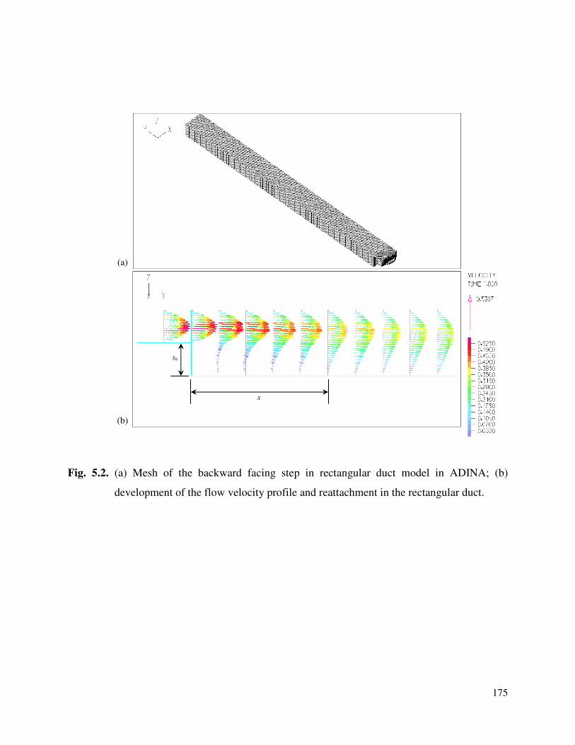
175
Fig. 5.2. (a) Mesh of the backward facing step in rectangular duct model in ADINA; (b)
development of the flow velocity profile and reattachment in the rectangular duct.
(a)
(b)
x
sh
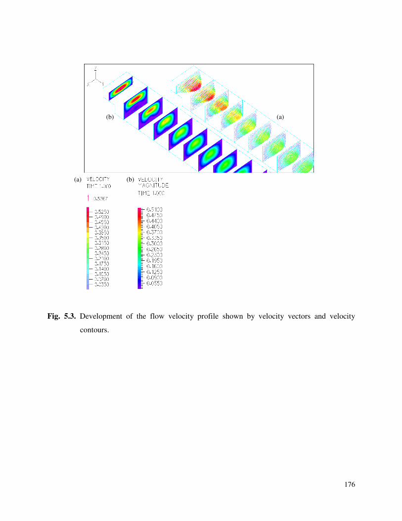
176
Fig. 5.3. Development of the flow velocity profile shown by velocity vectors and velocity
contours.
(b)
(b) (a)
(a)
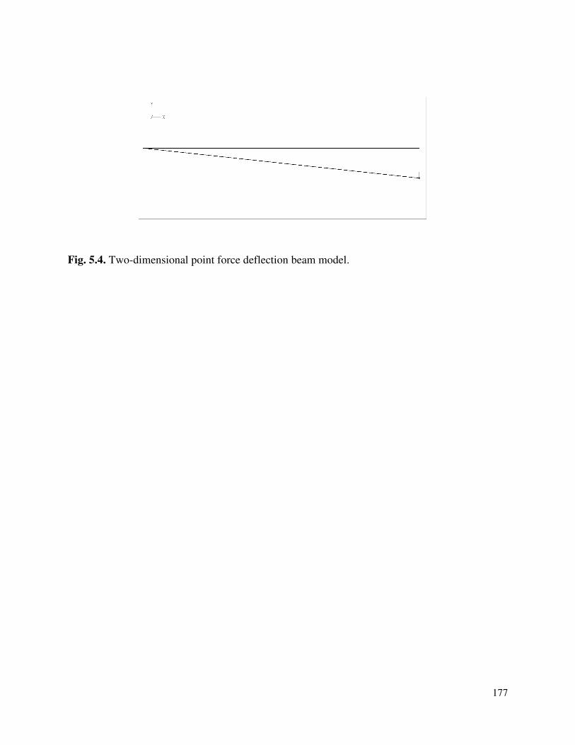
177
Fig. 5.4. Two-dimensional point force deflection beam model.
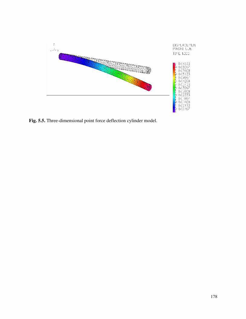
178
Fig. 5.5. Three-dimensional point force deflection cylinder model.
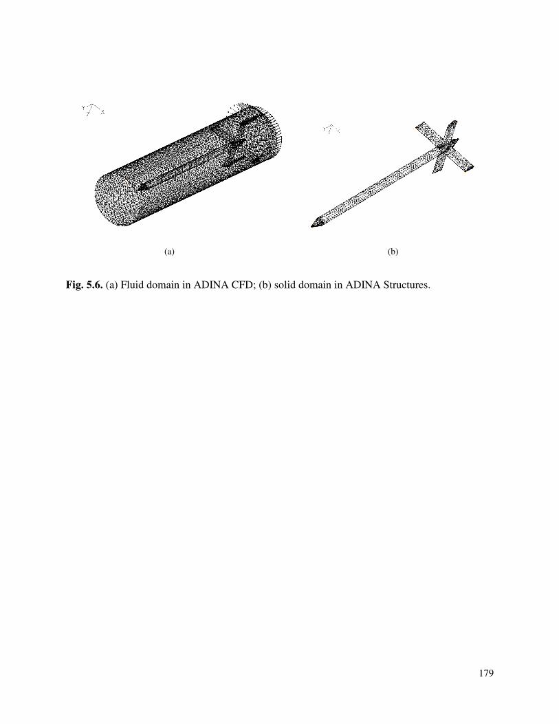
179
Fig. 5.6. (a) Fluid domain in ADINA CFD; (b) solid domain in ADINA Structures.
(a) (b)
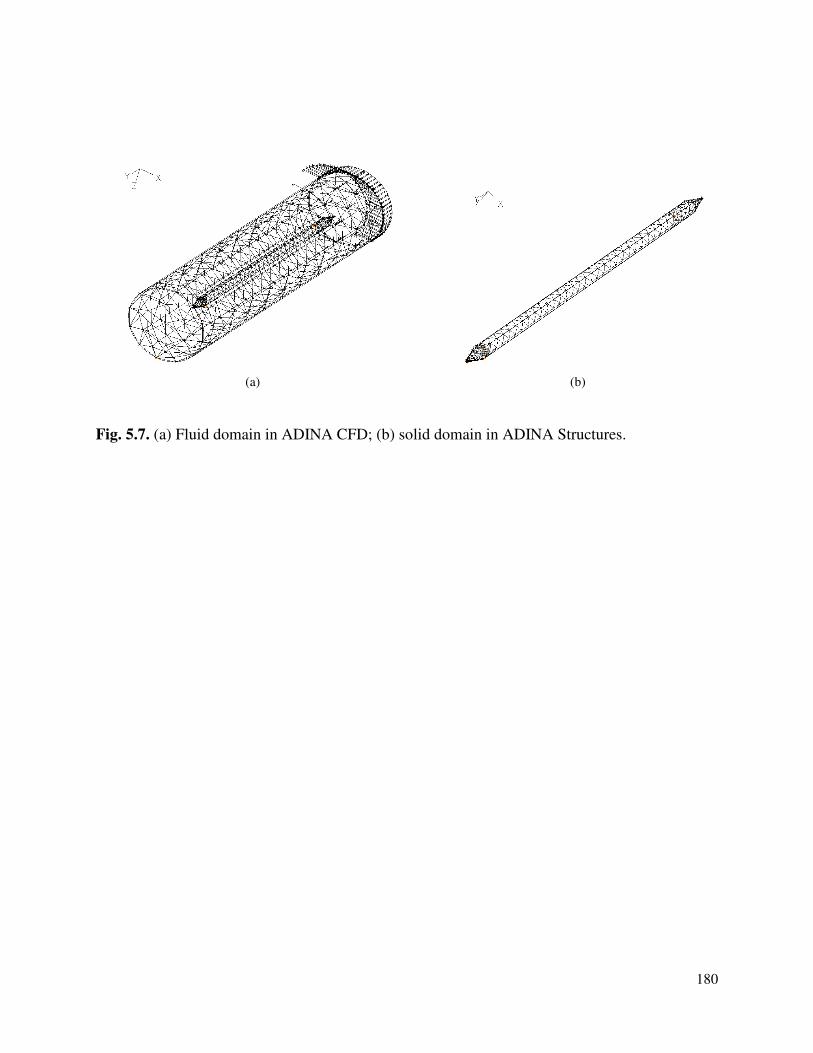
180
Fig. 5.7. (a) Fluid domain in ADINA CFD; (b) solid domain in ADINA Structures.
(a) (b)
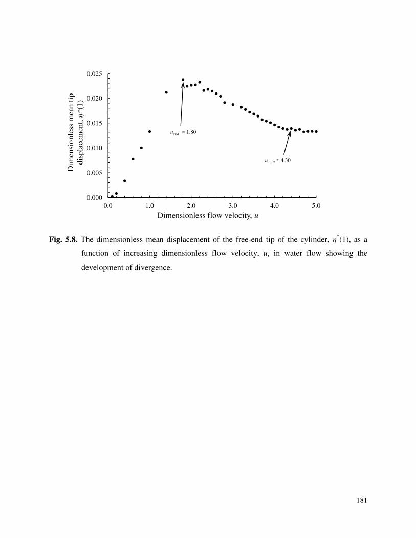
181
Fig. 5.8. The dimensionless mean displacement of the free-end tip of the cylinder, η*(1), as a
function of increasing dimensionless flow velocity, u, in water flow showing the
development of divergence.
0.000
0.005
0.010
0.015
0.020
0.025
0.0 1.0 2.0 3.0 4.0 5.0
Dim
ensi
onle
ss m
ean t
ip
dis
pla
cem
ent,
η*(1
)
Dimensionless flow velocity, u
ucr,d1 = 1.80
ucr,d2 ≈ 4.30
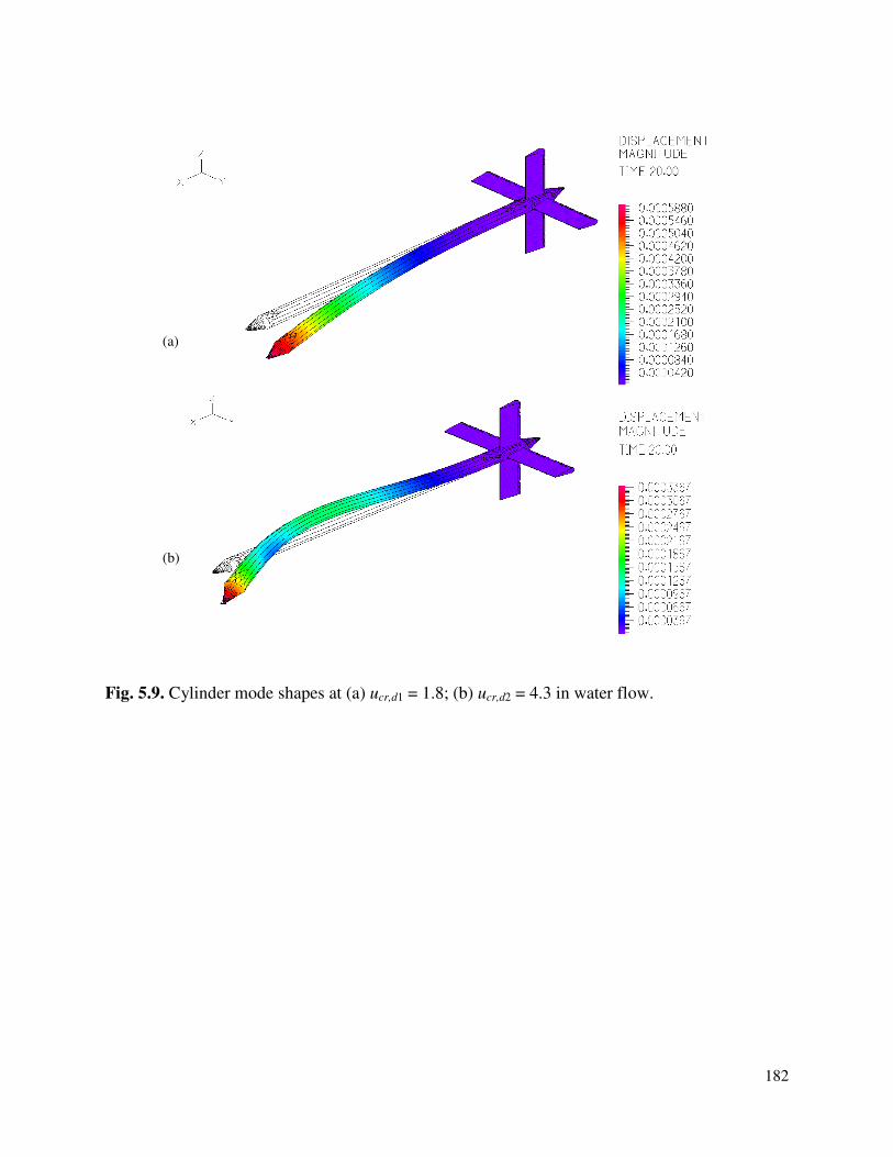
182
Fig. 5.9. Cylinder mode shapes at (a) ucr,d1 = 1.8; (b) ucr,d2 = 4.3 in water flow.
(a)
(b)
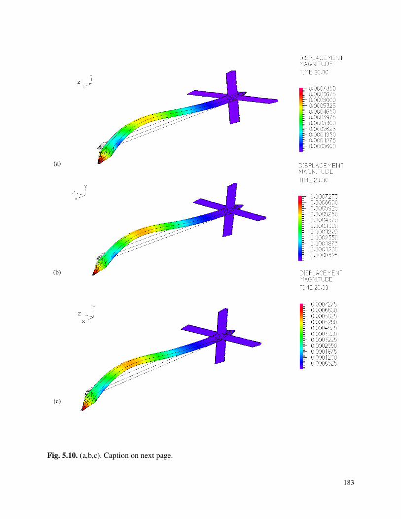
183
Fig. 5.10. (a,b,c). Caption on next page.
(b)
(c)
(a)
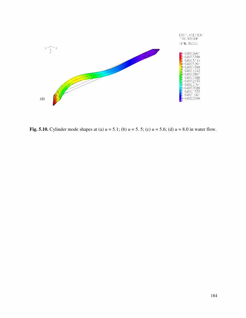
184
Fig. 5.10. Cylinder mode shapes at (a) u = 5.1; (b) u = 5. 5; (c) u = 5.6; (d) u = 8.0 in water flow.
(d)
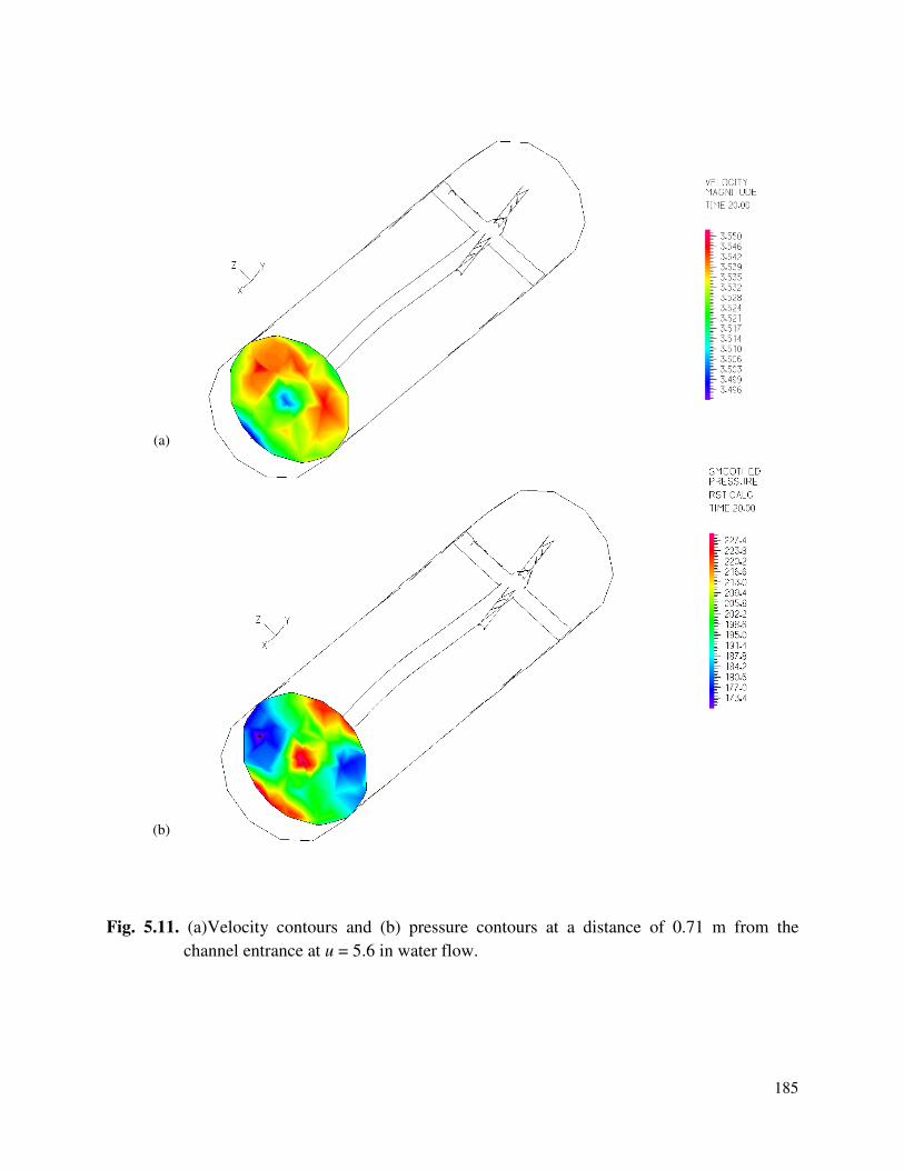
185
Fig. 5.11. (a)Velocity contours and (b) pressure contours at a distance of 0.71 m from the
channel entrance at u = 5.6 in water flow.
(a)
(b)
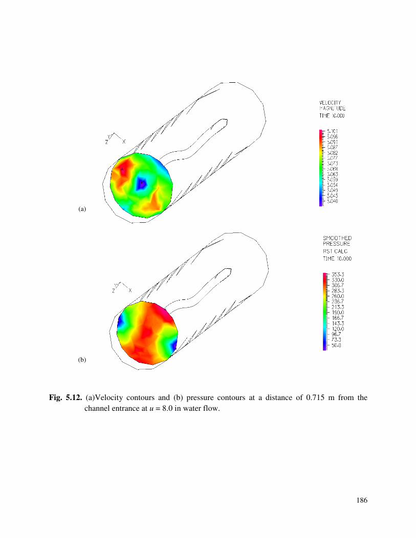
186
Fig. 5.12. (a)Velocity contours and (b) pressure contours at a distance of 0.715 m from the
channel entrance at u = 8.0 in water flow.
(a)
(b)
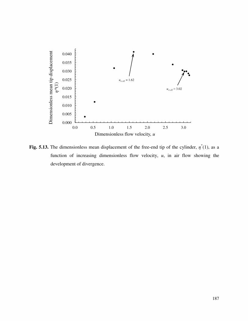
187
Fig. 5.13. The dimensionless mean displacement of the free-end tip of the cylinder, η*(1), as a
function of increasing dimensionless flow velocity, u, in air flow showing the
development of divergence.
0.000
0.005
0.010
0.015
0.020
0.025
0.030
0.035
0.040
0.0 0.5 1.0 1.5 2.0 2.5 3.0
Dim
ensi
onle
ss m
ean t
ip d
ispla
cem
ent
η*(1
)
Dimensionless flow velocity, u
ucr,d1 = 1.62
ucr,d2 ≈ 3.02
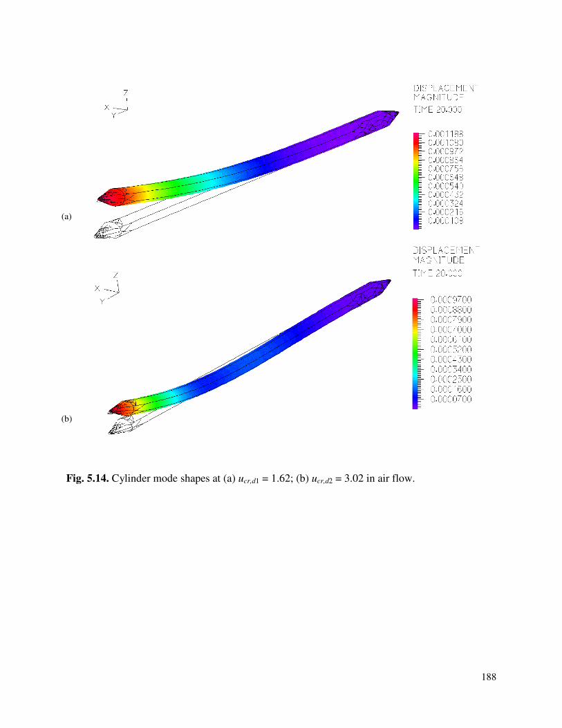
188
Fig. 5.14. Cylinder mode shapes at (a) ucr,d1 = 1.62; (b) ucr,d2 = 3.02 in air flow.
(b)
(a)
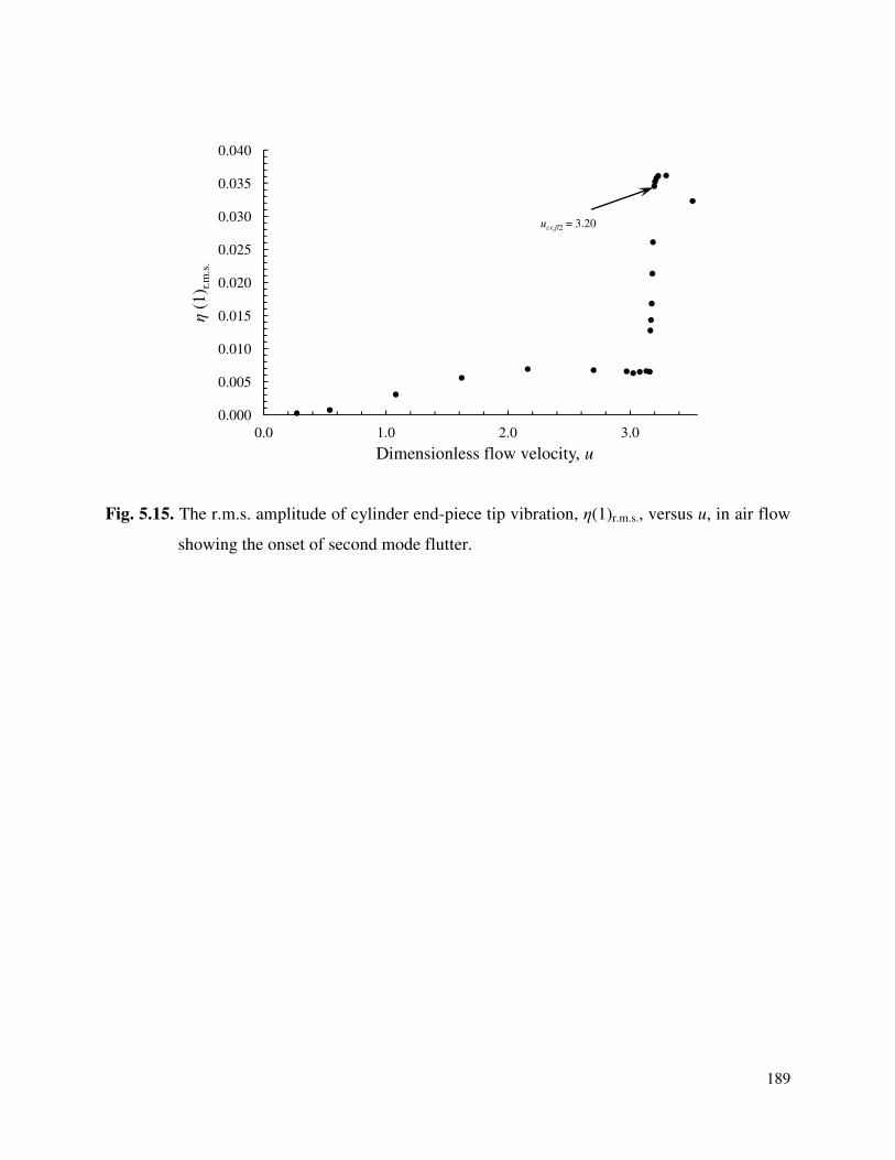
189
Fig. 5.15. The r.m.s. amplitude of cylinder end-piece tip vibration, η(1)r.m.s., versus u, in air flow
showing the onset of second mode flutter.
0.000
0.005
0.010
0.015
0.020
0.025
0.030
0.035
0.040
0.0 1.0 2.0 3.0
η(1
) r.m
.s.
Dimensionless flow velocity, u
ucr,fl2 = 3.20
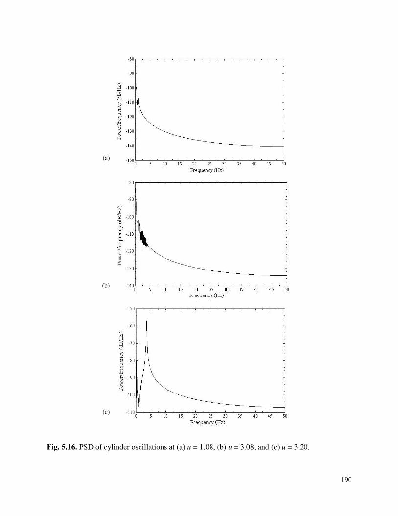
190
Fig. 5.16. PSD of cylinder oscillations at (a) u = 1.08, (b) u = 3.08, and (c) u = 3.20.
(b)
(a)
(c)
Chapter 6
Comparison of the Models
6.1. Introduction
In this chapter, the results in terms of critical flow velocities for the onset of static and dynamic
instabilities obtained from linear and nonlinear models, experiments and the numerical model in
water and air flows using the previously used and presently calculated force coefficients are
compared with each other. All the models are run for a cantilevered cylinder with an end-piece at
the downstream end. Experiments were conducted in a vertical test-section water tunnel. The
comparison gives a good picture of the dynamics of cantilevered cylinders in axial flow
investigated by different models and helps to understand the phenomena better by reasoning any
discrepancies present in the results.
6.2. Comparison of the Linear and the Nonlinear Models in Water and Air Flows with
Previously Used Force Coefficients
The results of linear and nonlinear models employing the force coefficients previously used by
Paїdoussis (1973) are compared with each other in this section. The results of the linear and
nonlinear models employing the previous force coefficients are presented and discussed in
Chapters 2 and 3, respectively. Table 6.1 shows these results in terms of critical flow velocities
for the onset of static and dynamic instabilities. Qualitatively, quite similar dynamical behaviors
of the cylinder are observed in the linear and nonlinear solutions subjected to water flow with the
exception of the evolution of second mode divergence not observed in the linear model. Third
mode flutter is not observed in the nonlinear results but one can expect it to occur after the flow
velocity, i.e., u = 7.70. For the linear model in air flow, third mode flutter is not observed. It may
be inferred that the energy transfer from air to the cylinder is not sufficient to excite the cylinder
in third mode.
Quantitatively, for models in water flow, the linear model exhibits higher critical flow
velocity for first mode divergence, ucr,d1, i.e., 2.042 as compared to 1.95 for the nonlinear one,
whereas nonlinear model shows higher ucr,fl2, i.e., 5.18 as compared to 5.173 for the linear one.
The overall maximum deviation is not more than 4.7 %. Linear model in air flow has the same
192
ucr,d1, whereas lower ucr,fl2 than the one in water flow. These observations are explained in
Chapter 3. Finally, the results of the model in air flow show the occurrence of second mode
divergence at ucr,d2 > ucr,fl2. This late occurrence of second mode divergence is explained in
Chapter 3. The comparison of the model results in water flow is also illustrated in Fig. 6.1.
6.3. Comparison of the Models in Water and Air Flows with Presently Calculated Force
Coefficients
The results from linear and nonlinear models, experiments, and numerical models in water flow
are compared in this section. In addition, numerical model results in air flow are also presented.
All the results, in this section, are obtained by employing the presently calculated force
coefficients. The present force coefficients are calculated using a three-dimensional model
generated in ADINA based on the input parameters matching those of experiments, meaning that
the coefficients represent closely the experiment conditions. That is why the results of
experiments and numerical model of ADINA are included in the comparison here in this section.
Table 6.2 shows these results in terms of critical flow velocities for the onset of static and
dynamic instabilities. Qualitatively, the linear and nonlinear models show coupled-mode flutter.
For both models, third mode flutter is not observed. One possible reason is that the linear model
becomes less accurate in predicting the dynamics well especially at high flow velocities, whereas
the nonlinear model solution becomes unstable at such high velocities to predict third mode
flutter. In addition, linear model does not show the transformation of first mode divergence into
the second mode. Also, second mode flutter is not observed in the numerical model; the reason
being the inherent numerical damping imposed on the cylinder, damping out the oscillations. For
the numerical model in air flow, third mode flutter is not observed up to the flow velocity, u =
3.51. It is expected to observe it as the flow velocity increases further but at flow velocities
higher than 3.51, the solution becomes more prone to becoming numerically unstable and the
program crashes.
Quantitative comparison show that ucr,d1 for models in water flow show good agreement
with discrepancies up to 3.74 %. The critical flow velocities, ucr,d2, for the models are reasonably
close with the maximum deviation up to 7.7 %. The critical flow velocities for coupled-mode
flutter, i.e., ucr, fl1,2, for the linear and nonlinear models are in good agreement with each other.
However, ucr, fl2 from experiments differs substantially. For experiments and numerical model,
193
ucr,d1 is obtained by arbitrarily choosing a threshold value of η*(1). The numerical model in air
flow shows lower ucr,d1, ucr,d2, and ucr,fl2 than their counterparts for the models in water flow. This
is explained in Chapter 5. The comparison of the model results in water flow is also illustrated in
Fig. 6.2.
It is known that the cantilevered cylinder is a non-conservative system. Such a system is
an open dissipative system, which means that mechanical energy may enter or leave the system.
The state of the system depends on how the system is subjected to the forces such as the inviscid
non-conservative and frictional forces. The frictional forces transform a small part of the
mechanical energy of the system such as the kinetic energy into heat, which leaves the system
and is lost. Therefore, the mechanical energy is not conserved when non-conservative forces are
present. The dynamics of the cantilevered cylinder depends on how these forces are formulated
and solved. The linear model of such cantilevered system has these forces formulated by
considering only the linear terms, making it less accurately predictive specifically in the post-
divergence velocity range. In nonlinear cylinder model, these forces are formulated, more
accurately by considering the nonlinear terms too, making it a better predictive tool for the
dynamics than the linear model. The numerically simulated model in ADINA is also nonlinear
with relatively less control on the formulation of the forces and any modification in the model
equation. Experiments, on the other hand, have no simplifying assumptions. The numerical
schemes employed to solve the nonlinear and the numerical models also have some inherent
numerical error, which cannot be totally eliminated. Also, the linear and nonlinear models
account for the fluid forces in two-dimensions only, whereas the ADINA simulations and the
experiments consider the fluid forces in all three-dimensions. In addition, for the experiments,
the onset of divergence is not abrupt and the values chosen for the onset of flutter depend on the
increments of fluid velocity chosen for data recording. Hence, the above factors can possibly
explain the small discrepancies present in the model results.
The linear equation solution does not give the displacement amplitudes directly; rather
the results are in terms of the complex eigenfrequencies and the instabilities are identified by the
imaginary part. In the case of the nonlinear model, the results show the state of the system in
terms of the generalized coordinate, q1. However, in the case of the experiments and the
numerical model, the displacement is represented by η*, the mean dimensionless displacement or
ηr.m.s., the r.m.s. value of the dimensionless displacement. Experimental results show that ηr.m.s. of
194
second mode flutter either stays relatively constant or decreases with increasing flow velocity by
up to approximately 13 % at u = 7.4. Hence, it is observed that numerical model results show far
smaller values of η*(1) than those of experiments. A possible reason as explained earlier in
Chapter 5 is that the negative damping of the system somehow does not increase considerably in
ADINA, resulting in small magnitudes of cylinder motion.
The frequencies of flutter of the models are now compared. The linear model directly
provides the dimensionless frequency as the real part of the complex eigenfrequency, whereas
nonlinear and numerical models and experiments first provide the dimensional frequency, which
is rendered dimensionless by using eq. (3.62). The Experimental results show that dimensionless
second mode flutter frequency either stays relatively constant or decreases with increasing flow
velocity by up to approximately 5 % at u = 6.9, whereas the third mode flutter frequency stays
relatively constant with a minuscule variation of 0.2 %. It is observed that the dimensionless
frequencies obtained from linear model are far higher than the ones obtained from other models.
The reason is that the real part of the eigenfrequency is in fact the resonant frequency of the
system. On the other hand, the frequencies observed by experiments and nonlinear and numerical
models are the ones at which the system oscillates in that particular mode and flow velocity.
Lastly, observing the results of the linear and nonlinear models in water flow with
previous and present force coefficients reveal that for models with the present force coefficients,
divergence occurs earlier than for the models with the previous coefficients used by Paїdoussis
(1973). For flutter, the models with the present force coefficients show a coupled-mode flutter
occurring at higher critical flow velocity than that for the models with the previous coefficients.
This can be explained with the help of the end shape factor, f, and the base drag represented by
cb. As mentioned earlier in Chapter 3, a decrease in f and an increase in cb have opposing effects
on divergence while the same on flutter, i.e., decreasing f stabilizes the system for both
divergence and flutter, while increasing cb destabilizes and stabilizes for divergence and flutter,
respectively. Since the model with the present force coefficients has same f (0.8) and higher cb
(0.2024) than that with the previous force coefficients (cb = 0.0), we can say that the opposing
effect of increasing cb on divergence and flutter causes the system with the present force
coefficients to destabilize by divergence at lower ucr,d1 and by flutter at higher ucr,fl2. In addition
to this, the coalescing of first and second modes in the coupled-mode flutter also contributes in
the delay.
195
6.4. Summary
In this chapter, the critical velocities, ucr, obtained from linear and nonlinear models,
experiments, and numerical model in water and air flows using the previous and present force
coefficients were compared. Results from the models in water flow with the previous force
coefficients showed that linear and nonlinear models had the respective critical flow velocities
quite close to each other except that the nonlinear model could not go beyond u = 7.70 to show
third mode flutter because of numerical instability issues. The results of the models in water flow
with the present force coefficients showed reasonable agreement with each other except the
value of ucr,fl2 for experiments. In each of the linear and nonlinear models with present force
coefficients, a coupled-mode flutter was observed. In the numerical model and experiments, the
emergence of first mode divergence was not abrupt and some threshold had to be chosen to help
obtaining the critical flow velocities. The second mode divergence in nonlinear and numerical
models in water and air flows, and experiments in water flow was mainly based on visual
inspection. However, second and third mode flutters in the models could be precisely located
with the help of r.m.s. values of the dimensionless displacements and the frequencies of
oscillations. It was also noticed that for the linear models with the previous and the present force
coefficients, evolution of second mode divergence was not observed at all.
196
Table 6.1. Comparison of critical flow velocities of instability for different models in water and
air flows using previous force coefficients.
Fluid Models/instabilities
First mode
divergence,
ucr,d1
Second
mode
divergence,
ucr,d2
Second
mode
flutter,
ucr,fl2
Third
mode
flutter,
ucr,fl3
Water Linear 2.042 -- 5.173 8.311
Nonlinear 2.04 ≈ 4.40 5.18 --
Air Linear 2.042 4.965 3.470 --
197
Table 6.2. Comparison of critical flow velocities of instability for linear and nonlinear models in
water flow using present force coefficients.
Fluid Models/instabilities
First mode
divergence,
ucr,d1
Second mode
divergence,
ucr,d2
Second mode
flutter,
ucr,fl2
Third mode
flutter,
ucr,fl3
Water
Experimental 1.87 ≈ 4.66 5.92 7.70
Linear [prev.]
(impr. from prev.)
1.904 [2.04]
(80.12 %) --
5.278 [5.16]
(coupled-mode)
(15.51 %)
--
Nonlinear [prev.]
(impr. from prev.)
1.89 [2.10]
(91.30 %) ≈ 4.40
5.29 [5.5]
(coupled-mode)
(-50 %)
--
Numerical 1.80 ≈ 4.30 -- --
Air Numerical 1.62 ≈ 3.02 3.20 --
198
Fig. 6.1. Critical flow velocities, ucr versus the instabilities for different models in water flow
using previous force coefficients. , linear model; , nonlinear model.
1.0
2.0
3.0
4.0
5.0
6.0
7.0
8.0
9.0
1st mode div. 2nd mode div. 2nd mode flt. 3rd mode flt.
ucr
199
Fig. 6.2. Critical flow velocities, ucr versus the instabilities for different models in water flow
using present force coefficients. , experiments; , linear model; , nonlinear
model; , numerical model.
1.0
2.0
3.0
4.0
5.0
6.0
7.0
8.0
1st mode div. 2nd mode div. 2nd mode flt. 3rd mode flt.
ucr
Chapter 7
Conclusions
7.1. Overview
In this thesis, the nonlinear dynamics of a slender flexible cantilevered cylinder subjected to
external axial flow was studied, both theoretically and experimentally. An extensive literature
review in Chapter 1 revealed that a three-dimensional coupled nonlinear model for the flexible
cylinder had not been developed. The motivation behind the present research work was to
account for the three-dimensional nonlinear behaviour, important in the practical applications
such as nuclear power production, heat exchangers, undersea geological survey, and biomedical
science. In addition, the fluid force coefficients used previously by Paїdoussis (1973) and Semler
et al. (2002) were re-evaluated to find out if these coefficients actually were suitable for the
present model.
The objectives outlined in Chapter 1 were achieved by solving the linear and nonlinear
equations, simulating numerical models, and conducting experiments. Also, the force
coefficients were recalculated based on the present experimental input parameters and then
implemented in the linear and nonlinear equations. The linear and nonlinear equations, with
these presently calculated force coefficients incorporated, were then solved. In addition, the
effect of confinement on the dynamics of linear model was also investigated. To complement the
linear and nonlinear models, three-dimensional model of flexible cylinder with cantilevered
boundary conditions was developed in a Finite Element Method (FEM) based multiphysics
simulation software called ADINA. Finally, experiments were conducted and the results
obtained from analytical linear, nonlinear, and numerical models, all in water flow, were then
validated by comparing them with those from the experiments. The results showed reasonable
agreement. Some special runs of linear and numerical models were also conducted in air flow.
The model results were also compared with each other.
7.2. Summary of the Work
In the previous section, steps taken to achieve the objectives were mentioned briefly, while in
this section, a detailed enumeration is presented.
201
Series of experiments were conducted on the confined cantilevered cylinder in a vertical
test section of a water tunnel. Water flowed from top to bottom of the test section. The
downstream free end of the cylinder was fitted with a rigid ogival end-piece. The upstream end
was clamped to a central rigid cylindrical support with four perpendicular arms extending to the
wall of the test section. Before the experiments were conducted, the laser sensors, utilized to
record the displacements of the cylinder in the experiments, were calibrated for known linear
distances and their calibration curves were obtained. The essential parameters such as flexural
rigidity, EI, logarithmic decrements, δn, hysteretic damping constant, , and the dimensionless
viscoelastic damping constant, of the cylinder were then determined experimentally. The
flexural rigidity was determined by first exciting the cylinder in its first mode and finding out the
first mode natural frequency. Using this frequency and the set of expressions and table given by
Paїdoussis and Des Trois Maisons (1969), EI was calculated. In order to obtain the logarithmic
decrements, the cylinder was excited in its first, second, and third modes. The first mode
excitation was done the same way as done for EI. However, the second and third cylinder modes
were excited mechanically with the help of a crank-slider mechanism and hence the respective
natural frequencies were determined. The natural logarithm of the displacement data for each
mode was then plotted versus time and the slope of the decrement was calculated. Later dividing
the slopes by the respective frequencies led to δ1, δ2, and δ3. and were then calculated
using the expressions and the plots given by Paїdoussis and Des Trois Maisons (1969).
The controller ATR141 for the differential-pressure transducer (Huba-692) connected to
the Venturi flow meter on the main flow pipe and the centrifugal pump speed in terms of r.p.m.
were calibrated using a pitot-static tube and a mercury manometer. The pitot-static tube was
carefully inserted through the lower test section window to align its tip with the centre-line of the
test section. Its static and stagnation pressure ports were connected to the mercury column
manometer. In addition to this, readings of the pressure transducers across the Venturi meter,
fitted in the water tunnel, were also recorded with the help of the controller ATR141. The tunnel
was then run at given pump r.p.m. A calibration curve, establishing the relationship between the
ATR141 readings and the flow velocity, was finally obtained. The velocity profile inside the test
section was also obtained experimentally using Laser Doppler Anemometry (LDA). In order to
establish the velocity profile in close proximity to the test section wall, law of the wall for
turbulent flow was utilized. Finally, in order to determine ucr,d1 and ucr,d2, the laser beam was
*µ
*α
*µ *α
202
horizontally pointed on the cylinder near its downstream free end. Mean dimensionless
displacements were plotted against u and the critical velocities were determined by choosing a
threshold value. The critical flow velocities ucr,fl2 and ucr,fl3 were determined by placing the leaser
head horizontally near the cylinder upstream end. The r.m.s. values of the cylinder dimensionless
displacements led to distinct critical flow velocities for flutter. At the end, the path traced by the
cylinder was also mapped.
The calibration curves of the laser sensors were linear. The calibration curve of ATR141
readings and the flow velocity was of sixth order polynomial. The half-symmetric flow velocity
profile had some mismatching between the experiment and the theoretical values at y = 0.0029 m
due to the inherent experimental errors such as difficulty in controlling the uniform density of the
seeding particles in the flow, laser bean diffraction due to different fluid and solid media. In
addition to these, rounding off the data of both the experimental and theoretical results to some
significant figures also made the values differ from each other. The theoretical model did not
give the exact true values of velocity due to the imprecise usage of the relations in the viscous
sub-layers, which do not have distinct boundaries. While recording and observing the evolution
of cylinder displacements at increasing flow velocity, it was obvious that the onset of first and
second mode divergences were not abrupt. Therefore, a threshold value had to chosen, especially
for ucr,d1, which ensured significant displacements and hence could confidently be considered as
the onset of divergence. For flutter, the r.m.s. values of the dimensionless displacements showed
substantial variation of the values at the onsets of second and third mode flutters. The overall
response of the cylinder showed the onset of first instability by first mode divergence followed
by a gradual evolution into second mode divergence. The cylinder then lost stability again by
second mode flutter and later by third mode flutter. The path traced by the cylinder in both
second and third mode flutters was observed to be quasi-circular path. In third mode flutter, the
difference between the major and minor axes of the path was found to be more than in second
mode flutter, making the quasi-circular path more pronounced in the third mode flutter.
Linear equation of motion, derived by Paїdoussis (1973), was considered for a slender
flexible cylinder with cantilevered boundary conditions, having the downstream free end of the
cylinder terminated by an ogival end-piece. The equation was then simplified to second-order
Ordinary Differential Equation (ODE) and finally to an eigenvalue problem. In order to
accommodate the time- and flow velocity-dependent free end boundary condition, a procedure
203
namely the ‘extended Galerkin method’ was adopted. The eigenvalue problem was then coded in
MATLAB and solved, using six Galerkin modes, for the complex eigenfrequencies comprising
of the resonant frequency as its real part and the damping as its imaginary part. The force
coefficients previously used by Paїdoussis (1973) were used. The results in the form of critical
flow velocities for the onset of instabilities were obtained for water flow. The effect of
confinement on the cylinder dynamics was also studied. The solution of the equation in air flow
was also obtained. Furthermore, the fluid forces such as inviscid hydrodynamic forces, frictional
or viscous forces, and hydrostatic or pressure forces acting on the cantilevered cylinder were
considered and the associated viscous force coefficients such as longitudinal viscous coefficient,
cT, normal viscous coefficient, cN, base drag coefficient, cb, and zero-flow normal coefficient, c
were recalculated. The values of the present force coefficients were found to be within their
respective suitable ranges suggested by Paїdoussis (2004). These present force coefficients were
incorporated into the linear equation and obtained the results. The effect of confinement on the
dynamics of the cylinder with the present force coefficients was also investigated. Finally, the
present model results with previously available force coefficients were compared with those of
Paїdoussis (1973) who solved the equation by a different method. A comparison was also done
between the results obtained with the previous and present force coefficients and then between
the results with water and air flows.
The results for an isolated unconfined cantilevered cylinder showed that the free motions
were damped at small dimensionless flow velocity, u. At sufficiently high u, however, the
cylinder first loses stability by divergence in its first mode followed by re-stabilization and then
single second mode flutter. At further higher u, the model lost stability again by third mode
flutter. The results for the model in air flow showed that at sufficiently high u, it lost stability by
first mode divergence followed by second mode flutter. At further higher u, third mode flutter
did not occur rather second mode divergence and third mode divergence occurred. Increasing
confinement of the model in water flow resulted in a decrease in ucr,d1 as well as ucr,fl2. For the
model in air flow, increasing confinement resulted in the same trend as in water flow. The results
of the model with present force coefficients showed that with increasing u, the model first lost
stability by first mode divergence followed by re-stabilization. Later, it lost stability again by
coupled-mode flutter. The cylinder did not become unstable in the third mode. As for the effect
of confinement with present force coefficients, the model exhibited the same trend of ucr,d1 and
204
ucr,fl2 as observed in the model with previous force coefficients. The comparison of the results of
present model with the ones reported by Paїdoussis (1973), both having the previous force
coefficients, showed good agreement. Previous and present force coefficient results were also
compared. The results revealed that the model with the presently calculated force coefficients
exhibit similar dynamics as observed in the experiments, especially the coalesced first mode
divergence and second mode flutter as the coupled-mode flutter (combination of the two modes
leads to an asymmetric response also observed in Figs. 2.32 and 2.33 of Chapter 2). Hence, it can
be concluded that the linear model with the presently calculated force coefficients predicts the
dynamics of the system better than the one with the previously used ones. The comparison of
model in water flow with the one in air flow showed similar values of ucr,d1. However, ucr,fl2 for
the model in air flow was lower than that in water flow.
The nonlinear equation of motion, derived by Lopes et al. (2002), was considered for a
confined slender flexible cylinder with cantilevered boundary conditions, having the downstream
free end of the cylinder terminated by an ogival end-piece. Hamilton’s principle was utilized for
the derivation. Due to the time- and flow velocity-dependent free end boundary condition,
‘extended Galerkin method’ was used to transform the PDE into ODE. The force coefficients
previously used by Semler et al. (2002) were used. The obtained equation was then solved using
Houbolt’s Finite Difference Method (FDM) using a FORTRAN code. Six Galerkin modes were
considered in both the axial and transverse directions in the solution. The presently calculated
force coefficients were then incorporated into the nonlinear equation and the results sought.
It was observed in the results with the previous coefficients that with increasing u, the
cylinder first lost stability by first mode divergence followed by a gradual evolution into second
mode. The cylinder then re-stabilized for short range of u and again became unstable by second
mode flutter. Instability in third mode was not observed. The results of the present model were
compared with those obtained by Semler et al. (2002), both with previous force coefficients, and
showed good agreement. Finally, the present models with previous and present coefficients were
compared to understand how the force coefficients affect the critical flow velocities. The results
of the model with the present force coefficients showed similar sequence of instability
occurrences as for the model with the previously used force coefficients except that the former
model had higher critical flow velocities, typically 13.30 % and 4.68 % higher for divergence
and flutter, respectively, than the latter one.
205
A cantilevered cylinder model, possessing the same input parameters as for the model in
experiments, was developed in ADINA. The cylinder had its downstream free end terminated by
an end piece. The upstream support had two configurations one with the support arms and the
other without. The study started by first validating the software with the help of theoretical and
experimental results of the benchmark problems reported in the earlier work. The solution time
step range was them determined using the CFL condition. The simulations of the model were
first done in water flow followed by the simulations in air flow. The model in water flow had the
upstream support arms attached to the central rigid cylindrical support, whereas the model in air
flow was devoid of those. Finally, a comparison was done between both the models.
The results of all the benchmark problems obtained from ADINA were in good
agreement with the ones previously reported. The dynamics of the cylinder in water flow showed
that, with increasing flow velocity, the cylinder first lost stability by divergence in first mode
followed by the evolution of second mode. Flutter did not occur even at very high flow velocity.
The model without support arms in water flow was also tested to see if flutter occurs but the
results were the same. A possible reason might be due to the inherent numerical damping
imposed in ADINA on the solid that damped out the oscillations. The dynamics of the cylinder
in air flow was the same except that in this case the second mode flutter was actually observed.
The value of ucr,fl2 was decided based on the r.m.s. values of the dimensionless amplitudes of the
cylinder, which was sustained over sufficient period of time. Finally, the models in water and air
flow were compared. It was observed that all critical velocities in air flow were lower than their
counterparts in water flow.
The results in the form of the critical flow velocities of linear and nonlinear models,
experiments, and numerical model in water and air flows using the previous and present force
coefficients were compared with each other. It was noticed that for the linear model in water
flow, evolution of second mode divergence was not observed at all. The results of the models in
water flow with the present force coefficients showed reasonable agreement with each other
except the value of ucr,fl2 for experiments. In each of the linear and nonlinear models with present
force coefficients, a coupled-mode flutter was observed. In the numerical model and
experiments, the emergence of first mode divergence was not abrupt and some threshold had to
be chosen to help obtaining the critical flow velocities. The second mode divergence for
nonlinear and numerical models in water and air flows, and experiments in water flow was
206
mainly based on visual inspection. However, second and third mode flutter in the models could
be precisely located with the help of r.m.s. values of the dimensionless displacements and the
frequencies of oscillations. The results, overall, showed reasonable agreement.
7.3. Suggestions for Future Work
The main goal of this thesis was to investigate the dynamics of a cantilevered cylinder in water
and air flows with the help of analytical and numerical models, supported by experiments. Due
to the wide scope of the present research work, some suggestions for future research in the same
area can be given.
There is little or no work done on the experiments pertaining to investigating the
dynamics of a slender flexible cylinder in confined axial flow. Confinement can be achieved
either by considering the cylinder in the presence of adjacent cylinders or in close proximity to
the flow-containing channel. It is known that with increased confinement, pressure drop is
clearly not negligible and viscous effects of fluid on the cylinder and on the flow channel
become more pronounced. In fact, confinement case is often present in many practical
applications such as nuclear fuel rods bundled together, heat exchanger tubes, and angioplasty.
Therefore, it is worth investigating this area with different boundary conditions such as
cantilevered, pinned-pinned, and clamped-clamped.
Eccentricity is encountered in many applications possessing enclosed slender cylinders.
In angioplasty, it is almost impossible to keep the slender flexible catheter concentric inside the
artery. Also, in the drilling operations of oil and gas wells, mud is pumped from a surface mud
tank via the drill pipe (several kilometers in length), through nozzles in the rotating drill bit, and
back to the mud tank through the annular space between the well bore wall and the drill pipe. It
is extremely difficult to keep the drill pipe concentric inside the well bore. Since mud flows
upward out of the well bore, any eccentricity present in the annulus can induce motion in the drill
pipe and can seriously affect the drilling operation. Therefore, it is important to investigate, both
experimentally and theoretically, how the dynamical behavior of the slender flexible cylinder is
affected by eccentricity. With eccentricity, the eccentric annulus causes the fluid forces acting on
the cylinder to be non-symmetric and, therefore, an appropriate coordinate system must be
adopted to resolve these forces. A bipolar coordinate system is the most suitable for this purpose.
207
The other way to account for the eccentricity was adopted by Mateescu et al. (1994), who used a
coordinate transformation factor to account for the circumferential variation of the annulus.
It is also worth investigating the combined effects of confinement and eccentricity on the
response of a slender flexible cylindrical system placed inside a channel subjected to axial flow,
both experimentally and theoretically. Both cases (confinement and eccentricity), combined, are
expected to restrict the motion of the cylinder.
It is also suggested to investigate other boundary conditions for the flexible cylindrical
structure such as clamped-pinned as limiting case, both experimentally and theoretically. The
above mentioned boundary conditions can be swapped or the flow direction reversed to see if
there is any variation in the response of the cylinder from the first condition.
References
ADINA. 2012. ADINA Research and Development. Massachusetts:
http://www.adina.com/index.shtml.
AML Oceanographic. 2013. Seismic Array. Sidney:
http://www.amloceanographic.com/Technical-Demo/Seismic-Array_2.
Armaly, B.F., Durst, F., Pereira, J.C.F., and Schönung, B. 1983. Experimental and theoretical
investigation of backward-facing step flow. Journal of Fluid Mechanics 127, 473-496.
Batchelor, G.K. 1967. An Introduction to Fluid Dynamics. Cambridge: Cambridge University
Press.
Ben-Gal, Y., Weisz, G., Collins, M.B., Genereux, P., Dangas, G.D., Teirstein, P.S., Singh, V.P.,
Rabbani, L.E., Kodali, S.K., Sherman, W., Leon, M.B., and Moses, J.W. 2010. Dual catheter
technique for the treatment of severe coronary artery perforations. Catheterization and
Cardiovascular Interventions 75 (5), 708-712.
Blevins, R.D. 1984. Applied Fluid Dynamic Handbook. New York: Van Nostrand Reinhold.
Blevins, R.D. 1990. Flow-Induced Vibration 2
nd Edition. Malabar: Krieger Publishing company.
Bungartz, H. and Schäfer, M. eds. 2006. Fluid-Structure Interaction: Modelling, Simulation,
Optimization. Berlin, Heidelberg: Springer Verlag.
Chen, S.S. 1978. Cross-flow induced vibrations of heat exchanger tube banks. Nuclear
Engineering and Design 47, 67-86.
Chen, Y.N. 1970a. Turbulence-induced instability of fuel rods in parallel flow. Sulzer Technical
Review, Special Issue, 72-84.
Chen, Y.N. 1970b. Flow-Induced Vibration in Heat Exchangers, p. 57. New York: ASME.
Chen, S.S. and Wambsganss, M.W. 1972. Parallel-flow-induced vibration of fuel rods. Nuclear
Engineering and Design 18, 253-278.
Cook, R.D., Malcus, D.S., and Plesha, M.E. 1989. Concepts and Applications of Finite Element
Analysis. New York: Wiley.
209
Courant, R., Friedrichs, K, and Lewy, H. 1967. On the partial difference equations of
mathematical physics. IBM Journal of Research and Development 11 (2), 215-234.
Dantec Dynamics. 2004. Flowlite Installation and User’s Guide. Skovlunde.
De Langre, E., Paїdoussis, M.P., Doare, O., and Modarres-Sadeghi, Y. 2007. Flutter of long
flexible cylinders in axial flow. Journal of Fluid Mechanics 571, 371-389.
Dowling, A.P. 1988. The dynamics of towed flexible cylinders. Part 1: neutrally buoyant
elements. Journal of Fluid Mechanics 187, 507-532.
Drain, L.E. 1980. The Laser Doppler Technique. New York: John Wiley & Sons.
Fujita, K. and Ohkuma, A. 2010. Effect of structural and fluid characteristics on dynamic
stability of an elastic beam subjected to axial flow in a narrow passage. Proceedings of
ASME 2010 3rd
joint US-European Fluids Engineering Summer Meeting and 8th
International Conference on Nanochannels, Microchannels, and Minichannels FEDSM2010-
ICNMM2010, Montreal, Canada.
Fujita, K. and Shintani, A. 1999. Flow-induced vibration of the elastic rod due to axial flow:
Unstable phenomena of continuous flexible rod as the axisymmetric body. ASME Flow
Induced Vibration, PVP 389, 199-206.
Fujita, K. and Shintani, A. 2001. Axial leakage flow-induced vibration of the elastic rod as the
axisymmetric continuous flexible beam. Journal of Pressure Vessel Technology 123, 421-
428.
Fujita, K., Morikazu, H., and Shintani, A. 2007. A consideration on pre-and post-instability of an
axisymmetric elastic beam subjected to axial leakage flow. Journal of Fluids and Structures
23, 463-478.
Gagnon, J.O. and Paїdoussis, M.P. 1994a. Fluid coupling characteristics and vibration of
cylinder clusters in axial flow. Part 1: Theory. Journal of Fluids and Structures 8, 257-291.
Gagnon, J.O. and Paїdoussis, M.P. 1994b. Fluid coupling characteristics and vibration of
cylinder clusters in axial flow. Part 2: Experiments. Journal of Fluids and Structures 8, 293-
324.
210
Gorman, D.J. 1969. The Role of Turbulence in the Vibration of Reactor Fuel Elements in Liquid
Flow. Atomic Energy of Canada Report AECL-3371.
Gorman, D.J. 1971. An analytical and experimental investigation of the vibration of cylindrical
reactor fuel elements in two-phase parallel flow. Nuclear Science and Engineering 44 (3),
277-290.
Hannoyer, M.J. 1977. Instabilities of Slender, Tapered Tubular Beams Induced by Internal and
External Axial Flow. Ph. D. Thesis, McGill University, Montreal, Canada.
Hannoyer, M.J. and Paїdoussis, M.P. 1978. Instabilities of tubular beams simultaneously
subjected to internal and external axial flows. ASME Journal of Mechanical Design 100,
328-336.
Hawthorne, W.R. 1961. The early development of the Dracone flexible barge. Proceedings of the
Institution of Mechanical Engineers 175, 52-83.
Hilber, H.M., Hughes, T.J.R., and Tayler, R.L. 1977. Improved numerical dissipation for time
integration algorithms in structural dynamics. Earthquake Engineering and Structural
Dynamics 5, 283-292.
Hoerner, S.F. 1965. Fluid Dynamic Drag, 2
nd Edition. Brick Town, New Jersey: Hoerner Fluid
Dynamics.
Idel’chik, I.E. 1966. Handbook of Hydraulic Resistance. Translated from Russian, AEC-tr-6630,
Springfield, VA: United States Department of Commerce. Also 1986, New York:
Hemisphere.
Kaneko, S., Nakamura, T., Inada, F., and Kato, M. 2008. Flow-Induced Vibrations:
Classifications and Lessons from Practical Experiences. Amsterdam, Boston, London:
Elsevier.
Ko, P.L. 1997. Wear of power plant components due to impact and sliding. Applied Mechanics
Reviews 50, 387-411.
Langthjem, M.A. and Nakamura, T. 2007. Influence of swirl on the stability of a rod in annular
leakage flow. Journal of Fluids and Structures 23, 329-337.
211
Langthjem, M.A., Morita, H., Nakamura, T., and Nakano, M. 2006. A flexible rod in annular
leakage flow: Influence of turbulence and equilibrium offset, and analysis of instability
mechanisms. Journal of Fluids and Structures 22, 617-645.
Lee, D. and Kennedy, R.M. 1985. A numerical treatment of a mixed type dynamic motion
equation arising from a towed acoustic antenna in the ocean. Computers & Mathematics with
Applications 11, 807-816.
Li, D.-W, Kaneko, S., and Hayama, S. 2002. A study on annular leakage-flow-induced
vibrations. Journal of Fluids and Structures 16 (7), 909-930.
Lighthill, M.J. 1960. Note on the swimming of slender fish. Journal of Fluid Mechanics 9, 305-
317.
Lopes, J.L., Paїdoussis, M.P., and Semler, C. 2002. Linear and nonlinear dynamics of
cantilevered cylinders in axial flow. Part 2: The equations of motion. Journal of Fluids and
Structures 16 (6), 715-737.
Mateescu, D. and Paїdoussis, M.P. 1985. The unsteady potential flow in an axially variable
annulus and its effect on the dynamics of the oscillating rigid center-body. Journal of Fluids
Engineering 107, 421-427.
Mateescu, D. and Paїdoussis, M.P. 1987. Unsteady viscous effects on the annular-flow-induced
instabilities of a rigid cylindrical body in a narrow duct. Journal of Fluids and Structures 1,
197-215.
Matlab help file 2010. MATLAB 64 bit version 7.10.0.499.
Miller, S.L. and Childers, D.G. 2004. Probability and Random Processes: with Applications to
Signal processing and Communications. Boston: Elsevier Academic Press. Modarres- Sadeghi, Y. 2006. Nonlinear Dynamics of a Slender Flexible Cylinder to Axial Flow.
Ph. D. Thesis, McGill University, Montreal, Canada.
Modarres-Sadeghi, Y., Paїdoussis, M.P., and Semler, C. 2005. A nonlinear model or an
extensible slender flexible cylinder subjected to axial flow. Journal of Fluids and Structures
21, 609-627.
212
Modarres-Sadeghi, Y., Paїdoussis, M.P., and Semler, C. 2007. The nonlinear behavior of a
slender flexible cylinder pinned or clamped at both ends and subjected to axial flow.
Computers and Structures, 85, 1121-1133.
Morgan, R.A. and Walser, E. 2010. Handbook of Angioplasty and Stenting Procedures. London:
Springer-Verlag.
Naudascher, E. and Rockwell, D. 1990. Flow-Induced Vibrations – An Engineering Guide (C)
Movement-Induced Excitation, Sonderforschungsbereich 210, “Strömungsmechanische
Bemessungsgrundlagen für Bauwerke” SFB 210/A/65, Universität Karlsruhe.
Naudascher, E. and Rockwell, D. 1994. Flow-Induced Vibrations: An Engineering Guide.
Rotterdam: A. A. Balkema.
Ni, C.C. and Hansen, R.J. 1978. An experimental study of the flow-induced motions of a flexible
cylinder in axial flow. ASME Journal of Fluids Engineering 100, 389-394.
Nie, J.H. and Armaly, B.F. 2003. Reattachment of three-dimensional flow adjacent to backward-
facing step. Transactions of the ASME 125, 422-428.
Ortloff, C.R. and Ives, J. 1969. On the dynamic motion of a thin flexible cylinder in a viscous
stream. Journal of Fluid Mechanics 38, 713-720.
Paїdoussis, M.P. 1966a. Dynamics of flexible slender cylinders in axial flow. Part 1: Theory.
Journal of Fluid Mechanics 26, 717-736.
Paїdoussis, M.P. 1966b. Dynamics of flexible slender cylinders in axial flow. Part 2:
Experiments. Journal of Fluid Mechanics 26, 737-751.
Paїdoussis, M.P. 1973. Dynamics of cylindrical structures subjected to axial flow. Journal of
Sound and Vibration 29 (3), 365-385.
Paїdoussis, M.P. 1974. The dynamical behavior of cylindrical structures in axial flow. Annals of
Nuclear Science and Engineering 1, 83-106.
Paїdoussis, M.P. 1979. The dynamics of clusters of flexible cylinders in axial flow: Theory and
experiments. Journal of Sound and Vibration 65 (3), 391-417.
213
Paїdoussis, M.P. 1980. Flow-Induced Vibrations in Nuclear Reactors and Heat Exchangers
Practical Experiences and State of Knowledge. Berlin, Heidelberg, New York: Springer
Verlag.
Paїdoussis, M.P. 1981. Fluidelastic vibration of cylinder arrays in axial and cross flow: State of
the art. Journal of Sound and Vibration 76 (3), 329-360.
Paїdoussis, M.P. 1983. A review of flow-induced vibrations in reactors and reactor components.
Nuclear Engineering and Design 78 (1), 31-60.
Paїdoussis, M.P. 1987. Flow-induced instabilities of cylindrical structures. Applied Mechanics
Reviews 40 (2), 163-175.
Paїdoussis, M.P. 1993. 1992 Calvin Rice lecture: Some curiosity-driven research in fluid
structure interactions and its current applications. Transactions of the ASME 115, 2-14.
Paїdoussis, M.P. 1998. Fluid-Structure Interactions: Slender Structures and Axial Flow, Vol. 1.
London: Elsevier Academic Press.
Paїdoussis, M.P. 2004. Fluid-Structure Interactions: Slender Structures and Axial Flow, Vol. 2.
London: Elsevier Academic Press.
Paїdoussis, M.P. 2008. The canonical problem of the fluid-conveying pipe and radiation of the
knowledge gained to other dynamics problems across applied mechanics. Journal of Sound
and Vibration 310, 462-492.
Paїdoussis, M.P. and Curling, Ll.R. 1985. An analytical model for vibration of clusters of
flexible cylinders in turbulent axial flow. Journal of Sound and Vibration 98, 493-517.
Paїdoussis, M.P. and Pettigrew, M.J. 1979. Dynamics of flexible cylinders in Axisymmetrically
confined axial flow. Journal of Applied Mechanics 46, 37-44.
Paїdoussis, M.P. and Suss, S. 1977. Stability of a cluster of flexible cylinders in bounded axial
flow. Journal of Applied Mechanics 44, 401-408.
Paїdoussis, M.P., Chaubernard, J.P., Genadry, M.R., and El Barbir, K.N. 1983b. Dynamics of a
cluster of flexibly interconnected cylinders. Part 2: In axial flow. Journal of Applied
Mechanics 50, 429-435.
214
Paїdoussis, M.P., El Barbir, K.N., Genadry, M.R., and Chaubernard, J.P. 1983a. Dynamics of a
cluster of flexibly interconnected cylinders. Part 1: In vacuum. Journal of Applied Mechanics
50, 421-428.
Paїdoussis, M.P., Grinevich, E., Adamovic, D., and Semler, C. 2002. Linear and nonlinear
dynamics of cantilevered cylinders in axial flow. Part 1: physical dynamics. Journal of
Fluids and Structures 16 (6), 691-713.
Paїdoussis, M.P., Issid, N.T., and Tsui, M. 1980a. Parametric resonance oscillations of flexible
slender cylinders in harmonically perturbed axial flow. Part 1: Theory. Journal of Applied
Mechanics 47, 709-714.
Paїdoussis, M.P., Issid, N.T., and Tsui, M. 1980b. Parametric resonance oscillations of flexible
slender cylinders in harmonically perturbed axial flow. Part 2: Experiments. Journal of
Applied Mechanics 47, 715-719.
Paїdoussis, M.P., Mateescu, D., and Sim, W.G. 1990. Dynamics and stability of a flexible
cylinder in a narrow coaxial cylindrical duct subjected to annular flow. Journal of Applied
Mechanics 57, 232-240.
Pao, H.P. 1970. Dynamical stability of a towed thin flexible cylinder. AIAA Journal of
Hydronautics 4, 144-150.
Pope, S.B. 2000. Turbulent Flows. New York: Cambridge University Press.
Quinn, E.P. 1962. Vibration of Fuel Rods in Parallel Flow. U.S. Atomic Energy Commission
Report GEAP-4059.
Reavis, J.R. 1967. WVI-Westinghouse vibration correlation for maximum fuel-element
displacement in parallel flow. Transactions of the American Nuclear Society 10, 369-371.
Reavis, J.R. 1969. Vibration correlation for maximum fuel-element displacement in parallel
turbulent flow. Nuclear Science and Engineering 38 (1), 63-69.
Rinaldi, S. 2009. Experiments on the dynamics of cantilevered pipes subjected to internal and/or
external axial flow. M. Eng Thesis, McGill University.
215
Ryder, G.H. 1969. Strength of Materials, 3rd
Edition. Hong Kong: English Language Book
Society/Macmillan.
Schlichting, H. and Gersten, K. 2000. Boundary-Layer Theory, 8
th Edition. Berlin, Heidelberg,
New York: Springer Verlag.
Semler, C., Lopes, J.L., Augu, N., and Paїdoussis, M.P. 2002. Linear and nonlinear dynamics of
cantilevered cylinders in axial flow. Part 3: Nonlinear dynamics. Journal of Fluids and
Structures 16 (6), 739-759.
Shaughnessy Jr., E.J., Katz, I.M., and Schaffer, J.P. 2005. Introduction to Fluid Mechanics. New
York: Oxford University Press.
Sinyavskii, V.F., Fedotovskii, V.S. and Kukhtin, A.B. 1980. Oscillation of a cylinder in a
viscous liquid. Prikladnaya Mekhanika 16, 62-67.
Strang, G. 1994. Wavelets. American Scientist 82 (3), 250-255.
Sudarsan, K., Bhattacharyya, S.K., and Vendhan, C.P. 1997. An experimental study of
hydroelastic instability of flexible towed underwater cylindrical structures. Proceedings of
16th
OMAE Conference, Yokohama, Japan A, 73-80.
Tang, L. 2007. The dynamics of two-dimensional cantilevered flexible plates in axial flow and a
new energy-harvesting concept . Ph. D. Thesis, McGill University.
Taylor, G.I. 1952. Analysis of the swimming of long and narrow animals. Proceedings of the
Royal Society of London. Series A, Mathematical and Physical Sciences 214, 158-183.
Triantafyllou, G.S. and Chryssostomidis, C. 1985. Stability of a string in axial flow. ASME
Journal of Energy Resources Technology 107, 421-425.
Wang, L. and Ni, Q. 2009. Vibration of slender structures subjected to axial flow or axially
towed in quiescent fluid. Advances in Acoustics and Vibration 2009, 1-19.
White, F.M. 1974. Viscous Fluid Flow. London: McGraw-Hill, Inc.
White, F.M. 2003. Fluid Mechanics. New York: McGraw-Hill, Inc.
216
Williams, P.T. and Baker, A.J. 1996. Incompressible computational fluid dynamics and the
continuity constraint method for the three-dimensional Navier-Stokes equations. Numerical
heat transfer, Part B 29, 137-273.
Yeh, Y. and Cummins, H.Z. 1964. Localized fluid flow measurements with He-Ne laser
spectrometer. Applied Physics Letters 4 (10), 176-178.
Zdravkovich, M.M. 2003. Flow around Circular Cylinders, Applications, Vol. 2. Oxford:
Oxford University Press.
Appendix A
A.1. Determination of End-Shape Factor, f
In the experiment, the cantilevered cylinder downstream end is fitted with an ogival end-piece.
Paїdoussis (1966b, 2002) investigated, experimentally and theoretically, the effect of the end-
piece shape on the cylinder instability pattern. He found both experimentally and theoretically
that transforming the end-piece from a well streamlined shape to a blunt shape stabilizes the
system for both divergence and flutter. He characterised the perfectly streamlined shape by the
end-shape factor, f = 1 and the perfectly blunt one by f = 0. Since the shape of the end-pieces
represented by the end-shape factor, f, it becomes important to find the value of f both for
theoretical models and experiments. Hannoyer and Paїdoussis (1978) proposed the expression
( ),
4
422
2
ioe
e
DDs
sf
−+= (A.1)
where se is the axial variation in the end-piece cross-sectional area. se is dimensional quantity and
has the unit of length, i.e., m; Di and Do being the inner and outer diameters of a pipe conveying
fluid, respectively. In order to render eq. (A.1) dimensionless, the expressions
,L
see =χ (A.2)
,oD
L=ε (A.3)
and
o
i
D
D=δ (A.4)
are used (Paїdoussis 2004). Do is the external diameter of a pipe or cylinder. The dimensionless
form thus obtained is
( ).
14
4222
22
δχε
χε
−+=
e
ef (A.5)
218
For a cylinder, 0=δ and ( )2
io DD − in eq. (A.1) is replaced by 2
oD . Hence, the dimensional and
dimensionless expressions for a cylinder become
.14
4
4
422
22
22
2
+=
+=
e
e
oe
e
Ds
sf
χε
χε (A.6)
The end-piece used in the experiments resembles closest to an ellipsoidal shape. Hence, for an
ellipsoidal end-piece, Paїdoussis (2004) defined se as
.3
2lse = (A.7)
Here, l is the length of the end-piece. Do is the same as D as used in the present case as both
represent the external diameter of the cylinder. For the present experiments, the parameters
involved in determining f are L = 0.5265 m, Do = 0.0254 m, and l = 0.03462 m. Substituting the
values in the above expressions gives f = 0.8. This value of f is also going to be used in the linear
and nonlinear models.