1

THREE-DIMENSIONAL PHOTOACOUSTIC TOMOGRAPHY AND ITS APPLICATION TO DETECTION OF JOINT DISEASES IN THE HAND

By

YAO SUN

A DISSERTATION PRESENTED TO THE GRADUATE SCHOOL OF THE UNIVERSITY OF FLORIDA IN PARTIAL FULFILLMENT

OF THE REQUIREMENTS FOR THE DEGREE OF DOCTOR OF PHILOSOPHY

UNIVERSITY OF FLORIDA

2010

2

© 2010 Yao Sun

3

To my wife, Xiaorong Li;

My mom and my dad; And all who have been supportive to me in my life

4

ACKNOWLEDGMENTS

First, I would like to thank Professor Huabei Jiang, who provided this great

education opportunity to me. I appreciate the full financial support and precious advice I

have received from Professor Jiang during my study for the PhD degree. His broad

views and deep understandings on the research subjects guided me all through this

research. His awareness to timetable and duty priorities, and his persistence to

research objectives deeply impressed me. What I have learned and experienced in

Professor Jiang’s lab will definitely benefit my future career and life.

Secondly, my thanks go to my academic committee members: Dr. David Gilland,

Dr. Rosalind Sadleir, and Dr. Sihong Song. Their comments and suggestions were very

helpful to my study and research. Their valuable time spent on reading my dissertation

is highly appreciated.

Thirdly, I would like to thank Dr. Eric S. Sobel, an associate professor in the

College of Medicine at University of Florida. As our clinical research partner, Dr. Sobel

helps us to recruit sufficient patients with osteoarthritis. And I would like to thank the

research assistant professors in our lab, Dr. Qizhi Zhang and Dr. Zhen Yuan, for

valuable discussions on experiments and computations, respectively.

Last but not least, I would like to take this opportunity to express my thanks to Lei

Xi, Qiang Wang, Lei Yao, Yiyong Tan, Ruixin Jiang, Alexandria Grubbs, Xiaoping Liang,

Lu Yin, Lijun Ji, Bo Wang, and all members in our biomedical optics lab for their

assistance and the great time we spent together.

5

TABLE OF CONTENTS page

ACKNOWLEDGMENTS.................................................................................................. 4

LIST OF TABLES............................................................................................................ 7

LIST OF FIGURES.......................................................................................................... 8

LIST OF ABBREVIATIONS........................................................................................... 12

ABSTRACT ................................................................................................................... 13

CHAPTER

1 BACKGROUND AND SIGNIFICANCE ................................................................... 16

1.1 Introduction to Photoacoustic Tomography....................................................... 16 1.2 Overview of Osteoarthritis................................................................................. 18

2 RECONSTRCUTION ALGORITHM IN PAT ........................................................... 24

2.1 Finite Element Based Reconstruction Algorithm in PAT ................................... 24 2.1.1 Forward Modeling in Acoustically Homogenous Media ......................... 26 2.1.2 Inverse Modeling and Nonlinear Optimization in PAT Reconstruction .. 27 2.1.3 Regularization in PAT Reconstruction................................................... 30 2.1.4 Simulation in PAT Reconstruction ......................................................... 33

2.2 Computing Strategies in PAT Reconstruction................................................... 33 2.2.1 Adjoin Sensitivity Method ...................................................................... 34 2.2.2 Dual Meshing Scheme .......................................................................... 34 2.2.3 Partial Reconstruction in Region of Interest .......................................... 37 2.2.4 Parallel Computing Technique .............................................................. 39

3 PRE-INVESTIGATION OF 3-D PAT SYSTEM WITH TISSUE PHANTOM STUDY 47

3.1 Tissue Mimicking Phantom ............................................................................... 48 3.2 System Description and Experiments ............................................................... 49 3.3 Methods ............................................................................................................ 50 3.4 Results and Discussion..................................................................................... 52

4 IMAGING FINGER JOINTS IN-VIVO WITH 3-D PAT IN A SPHERICAL SCAN..... 63

4.1 System Development and Description .............................................................. 63 4.1.1 Fiber Guided Near Infrared Lighting ...................................................... 64 4.1.2 Arrangement for Hand and Finger Placement....................................... 65 4.1.3 Signal Detecting in a Spherical Scanning Geometry ............................. 65 4.1.4 Units Control and Data Acquisition System........................................... 67

6

4.2 In-vivo Experiments .......................................................................................... 67 4.3 Methods ............................................................................................................ 68 4.4 Results and Discussion..................................................................................... 69

5 CLINCAL EXAMINATION OF OA PATIENTS WITH 3-D PAT................................ 79

5.1 Enhancement in 3-D PAT Approach ................................................................. 80 5.1.1 Ultrasound Detection Array ................................................................... 81 5.1.2 Multiple Channel Data Acquisition......................................................... 83 5.1.3 Quantitative 3-D PAT with 3-D Photon Diffusion Model ........................ 83 5.1.4 Tissue-like Phantom Test...................................................................... 84

5.2 Patients and Clinical Data................................................................................. 85 5.3 Results.............................................................................................................. 86 5.4 Discussion ........................................................................................................ 89

6 IN-VIVO IMAGIING of CHROMOPHORE CONCENTRATIONS in FINGER JOINTS WITH MULTISPECTRAL 3-D PAT.......................................................... 100

6.1 Methods .......................................................................................................... 102 6.2 In-vivo Experiments ........................................................................................ 104 6.3 Results and Discussion................................................................................... 105

7 CONCLUSION AND FUTHER WORK.................................................................. 115

7.1 Conclusion ...................................................................................................... 115 7.2 Future Studies ................................................................................................ 116

7.2.1 Evaluation of 3-D PAT in OA Detection with Small Clinical Samples .. 116 7.2.2 In-vivo Detection of Rheumatoid Arthritis in the Hand......................... 116 7.2.3 Recover Acoustic Property Together with Optical Properties by PAT

Approach ........................................................................................... 117

LIST OF REFERENCES ............................................................................................. 121

BIOGRAPHICAL SKETCH.......................................................................................... 128

7

LIST OF TABLES

Table page 3-1 Phantoms used in the pre-investigation of 3-D PAT system............................... 56

5-1 Averaged absorption coefficient and size of joint tissues for 2 OA and 4 normal joints ....................................................................................................... 99

8

LIST OF FIGURES

Figure page 1-1 Schematic of photoacoustic effect. ..................................................................... 23

2-1 The reconstructed images for simulated finger joint (a) coronal section slice along X=0mm (b) cross section slice along Z=15mm. ........................................ 42

2-2 Geometry of the absorbed energy interpolation at fine node i in 2-D case (a) and in 3-D case (b), and the calculation of the Jacobian matrix element in the effective integration zone (c). ............................................................................. 42

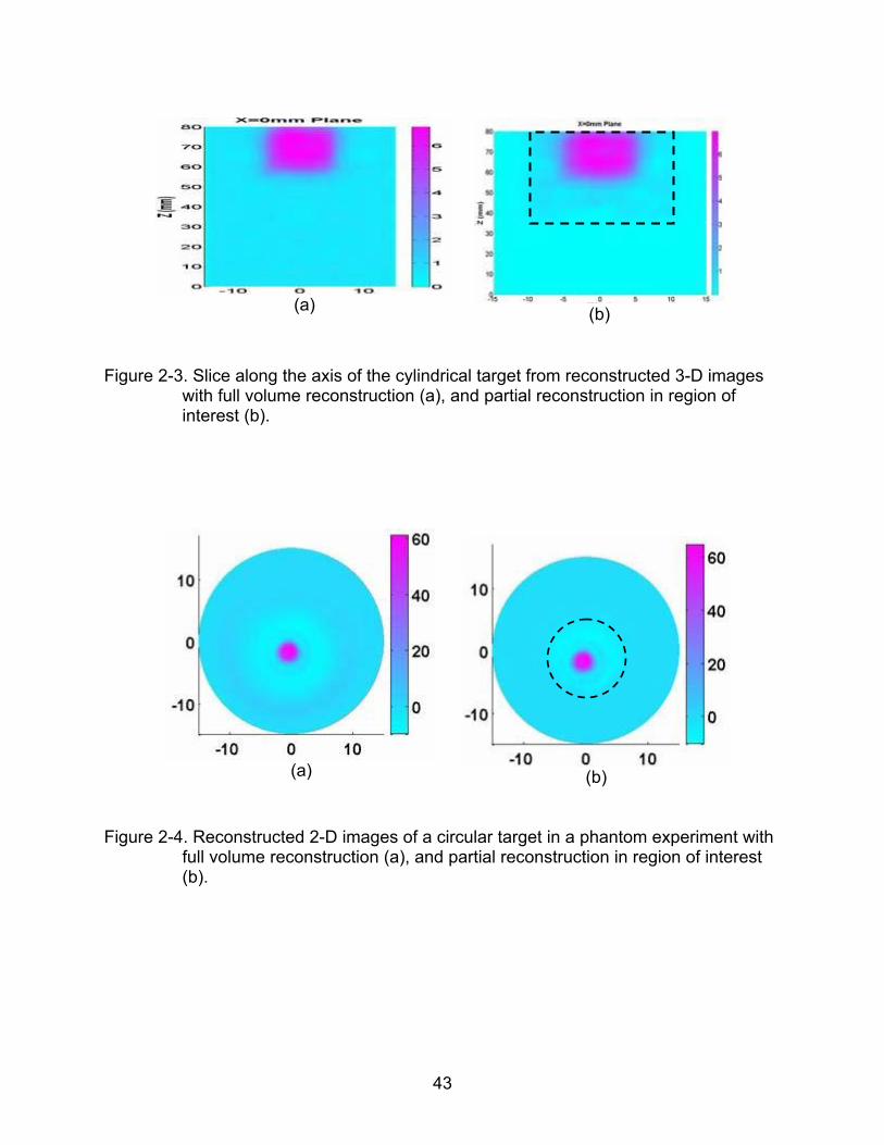
2-3 Slice along the axis of the cylindrical target from reconstructed 3-D images with full volume reconstruction (a), and partial reconstruction in region of interest (b). ......................................................................................................... 43

2-4 Reconstructed 2-D images of a circular target in a phantom experiment with full volume reconstruction (a), and partial reconstruction in region of interest (b). ...................................................................................................................... 43

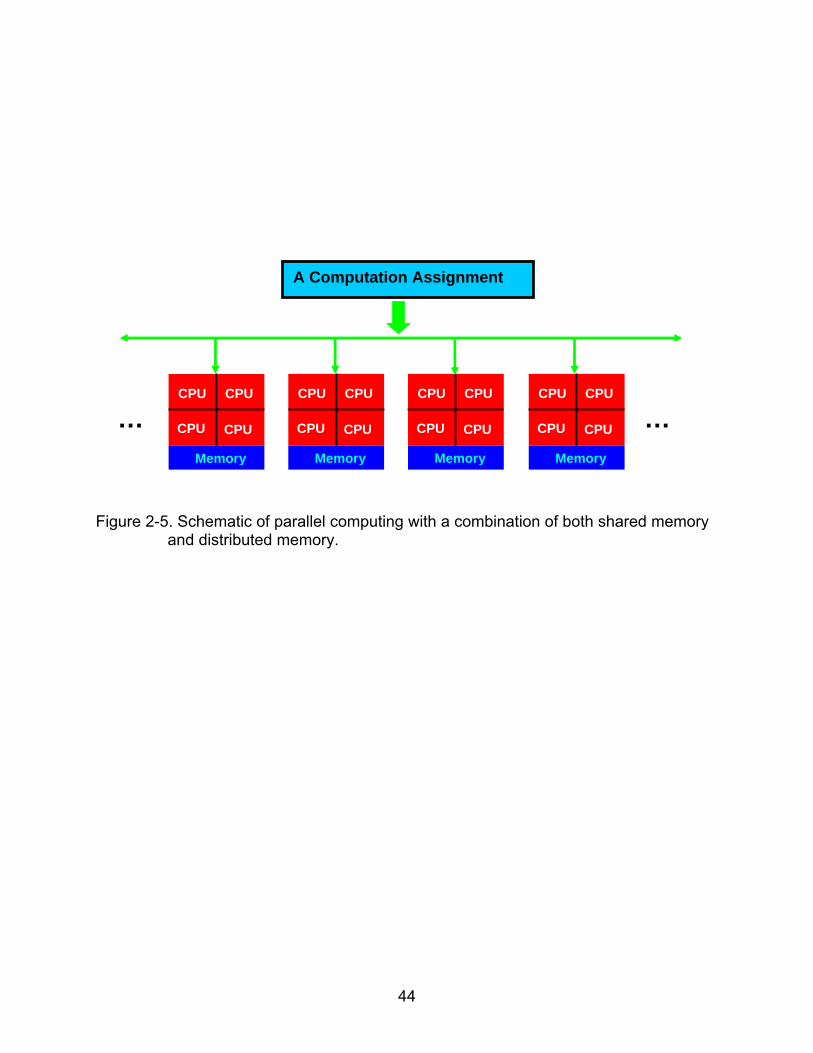
2-5 Schematic of parallel computing with a combination of both shared memory and distributed memory. ..................................................................................... 44

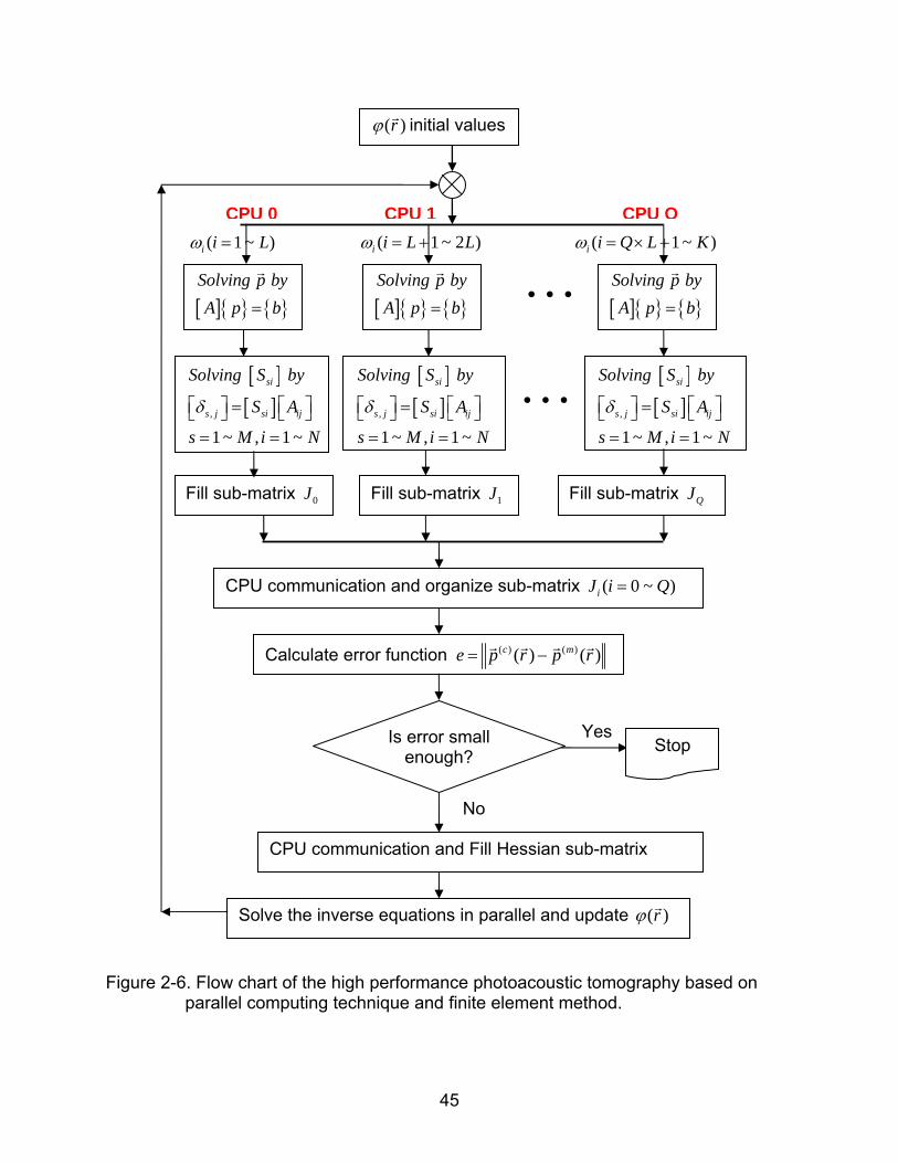
2-6 Flow chart of the high performance photoacoustic tomography based on parallel computing technique and finite element method.................................... 45

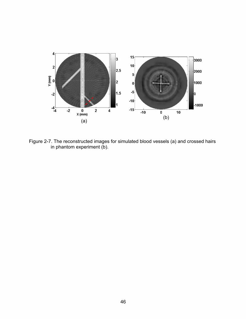
2-7 The reconstructed images for simulated blood vessels (a) and crossed hairs in phantom experiment (b).................................................................................. 46

3-1 Schematic of two potential cylindrical scanning geometries of finger joints imaging in 3-D PAT. ........................................................................................... 57

3-2 A slice through the axis of the reconstructed finger joint scanned by a cylindrical geometry shown in Figure 3-1(b) ....................................................... 57

3-3 Schematic of the three-dimensional photoacoustic imaging system................... 58

3-4 Schematic of the scanning arc/path in the XY plane. ......................................... 58

3-5 Reconstructed absorbed energy density images in the coronal (z=0mm), sagittal (x=0mm) and cross (y=4mm) sections for a joint-like phantom with 1mm thick cartilage in cylindrical (a) and spherical (b) scanning geometries, and with 2mm thick cartilage in spherical scanning geometry (c). ...................... 59

3-6 Reconstructed absorption coefficient images (coronal section) for the phantom with 1mm (a) and 2mm (b) thick cartilage............................................ 60

9

3-7 The recovered absorption coefficient distributions along a transect (x=0mm) for the images shown in Figure 3-6. ................................................................... 60

3-8 Reconstructed absorbed energy density images in the coronal (z=0mm), sagittal (x=0mm) and cross (y=4mm) sections for a joint-like phantom where the absorption coefficient of cartilage was 0.015 (a), 0.025 (b), 0.03 (c) and 0.04 (d) mm-1. ..................................................................................................... 61

3-9 Reconstructed absorption coefficient images (coronal section) for the phantom with an absorption coefficient of cartilage of 0.015 (a), 0.025 (b), 0.03 (c) and 0.04 mm-1 (d). ................................................................................. 62

3-10 The recovered absorption coefficient distributions along a transect (x=0mm) for the images shown in Figure 3-9. ................................................................... 62

4-1 Schematic of the 3-D spherical scanning PAT system for finger joint imaging. .. 72

4-2 Test of lighting beam with a cylindrical phantom (a), a line phantom (b), and a pencil lead (c). .................................................................................................... 72

4-3 Photograph of the arrangement for hand and finger Placement. ........................ 73

4-4 Schematic of the spherical scanning geometry (a), circular locus L1 (b) and L2 (c). ................................................................................................................. 73

4-5 Reconstruction mesh and possible model mismatch of 2-D circular scanning (a) and 3-D spherical scanning (b). .................................................................... 74

4-6 Bubble level gauge (a) and homemade marker cap (b) for calibration of mechanical errors in the photoacoustic spherical scanner. ................................ 74

4-7 A selected coronal section from the reconstructed 3-D image (absorbed energy density) at Z=-5mm (a), and MRI (coronal section) from a similar joint (b).. ..................................................................................................................... 75

4-8 A selected coronal section from the recovered absorption coefficient image at Z=-5mm (a), and its profile along the cut line X=-2mm (b). ................................ 75

4-9 A selected cross section from the reconstructed 3-D image (absorbed energy density) at Y=7mm (a), and MRI (cross section) from a similar joint (b).. ........... 76

4-10 A selected cross section from the recovered absorption coefficient image at Y=7mm (a), and its profile along cut lines 1 (b) and 2 (c), respectively. ............. 76

4-11 Cross section images (absorbed energy density) at Y=-2.5mm (a), Y=0mm (b), Y=3mm (c), Y=5mm (d), Y=7mm (e) and Y=9mm (f).. ................................. 77

10

4-12 Coronal section images (absorbed energy density) at Z=-5mm (a), Z=-3.5mm (b), Z=1mm (c) and Z=4.5mm (d). ...................................................................... 78

5-1 Photograph of the transducer array/finger interface of the three-dimensional photoacoustic tomography system used for the current study............................ 92

5-2 Geometry of the detector array........................................................................... 92

5-3 An example of possible mismatches between the center of the detector array (marked as O) and the rotary center of the rotary stage R2 (marked as O’)....... 93

5-4 Alignment variations (a) and spectrum differences in impulse responses of four selected transducer elements in the ultrasound detecting array.................. 93

5-5 Block diagram of the multiple-channel 3-D PAT system..................................... 94

5-6 The central values of the 16 channels in PCIAD1650 card (a) and Labview control interface (b) in multiple-channel 3-D PAT system................................... 95

5-7 Reconstructed optical absorption coefficient images in the coronal (z=0.0mm) and sagittal (x=0mm) sections as well as in 3-D view for a joint-like phantom where the absorption coefficient of “cartilage” was 0.01 (a) and 0.03mm-1 (b). (c) shows the recovered absorption coefficient distributions along a transect crossing the “bones” and “cartilage” (x=0.5mm) for the images in coronal section . ................................................................................. 96

5-8 Photographic schematic of the coronal (a) and sagittal (b) sections for the finger joint imaging. ............................................................................................ 97

5-9 Recovered images at selected coronal (a) / sagittal (b) planes for case 1 (Healthy). ............................................................................................................ 97

5-10 Recovered images at selected coronal (a) / sagittal (b) planes for case 5 (OA).................................................................................................................... 98

6-1 Absorption spectra of oxy-hemoglobin (HbO2), deoxy-hemoglobin (Hb) and water (H2O) in biological tissues....................................................................... 110

6-2 Homemade 3-D positioning ruler. ..................................................................... 110

6-3 Recovered optical absorption maps in coronal section (a) and sagittal section (b) of an in-vivo finger joint for light source in six wavelengths. ........................ 111

6-4 Concentrations of oxy-hemoglobin (a) and deoxy-hemoglobin (b) in M , and the water content (c) at coronal section (z=-8mm) and sagittal section (x=-1mm) of examined finger joint from an OA patient. .......................................... 112

11

6-5 Concentrations of oxy-hemoglobin (a) and deoxy-hemoglobin (b) in M , and the water content (c) at coronal section (z=2mm) and sagittal section (x=-0.5mm) of examined finger joint from a healthy subject ................................... 113

6-6 Average Concentrations of oxy-hemoglobin(HbO2), total hemoglobin (Total-Hb) and the oxygen saturation (SO2) in finger joint bones (a) and in joint cavity (b). .......................................................................................................... 114

7-1 Reconstructed images at selected sagittal (a) / coronal (b) planes for an in-vivo PIP joint..................................................................................................... 119

7-2 Simulation geometry to recover ultrasound speed with PAT method. (a) is the simulation geometry of optical contrasts; (b) is the simulation geometry of ultrasound contrasts; ........................................................................................ 119

7-3 Reconstructed optical contrast images (A) and ultrasound speed images (B) at 1st iteration (a), 3rd iteration (b) and 5th iteration (c)....................................... 120

12

LIST OF ABBREVIATIONS

2-D Two-dimensional

3-D Three-dimensional

CT Computed tomography

DOT Diffuse Optical Tomography

DIP Distal Interphalangeal

FE Finite Element

MRI Magnetic Resonance Imaging

NIR Near-infrared

OA Osteoarthritis

PAT Photoacoustic Tomography

PIP Proximal Interphalangeal

qPAT Quantitative Photoacoustic Tomography

RA Rheumatoid Arthritis

US Ultrasonography

13

Abstract of Dissertation Presented to the Graduate School of the University of Florida in Partial Fulfillment of the Requirements for the Degree of Doctor of Philosophy

THREE-DIMENSIONAL PHOTOACOUSTIC TOMOGRAPHY AND ITS APPLICATION

TO DETECTION OF JOINT DISEASES IN THE HAND

By

Yao Sun

August 2010

Chair: Huabei Jiang Major: Biomedical Engineering

This thesis research presents the study of three-dimensional (3-D) photoacoustic

tomography (PAT) and its application for the first time to detection of osteoarthritis (OA)

in the hand. PAT is an emerging non-ionizing, non-invasive imaging modality that can

visualize high optical contrast in biological tissues with high ultrasound resolution.

Compared with other imaging modalities that have been conventionally used or recently

investigated to visualize the structural abnormalities in the finger joints with OA, the 3-D

PAT approach studied in this dissertation not only provides high-resolution anatomical

structures, but also offers quantitative tissue optical property as well as physiological /

functional information including concentrations of oxy-hemoglobin (HbO2), deoxy-

hemoglobin (Hb) and water (H2O) that could be used to detect OA in an early stage.

In this study, a 3-D high performance PAT reconstruction algorithm is developed

based on parallel computing technique and finite element method. The optimal detector

performance and scanning geometry for 3-D photoacoustic imaging of the finger joints

are investigated with considerable phantom experiments. The results of phantom

experiments show that a spherical scanning geometry appears to provide improved

spatial solution over a cylindrical scanning geometry, and that 1mm thick “cartilage” can

14

be accurately differentiated from the “bones” with a 1 MHz transducer in a spherical

scanning geometry. In addition, the absorption coefficient of the “cartilage” can be

effectively recovered when this optical property varied from 0.015mm-1 to 0.04mm-1. A

3-D PAT system in a spherical scanning geometry has been constructed and optimized

for in-vivo examination of human finger joints. A distal interphalangeal (DIP) joint from a

female healthy subject was photoacoustically examined by our 3-D PAT system, and

major anatomical structures of the examined DIP joint along with the side arteries were

clearly reconstructed in high quality, where joint space was well differentiated from

surrounding finger phalanges. The performance of the 3-D PAT system was further

improved with an ultrasound detection array composed of eight 1 MHz transducers and

a 16-channel pulse/receive board. The 8-channel 3-D PAT system was carefully

calibrated with controlled tissue phantom experiments, and is capable of completing a

finger joint examination within 5 minutes (at single optical wavelength).

The 3-D PAT reconstruction algorithm and scanning system developed has also

been applied to a pilot clinical study aiming to test the possibility of detecting OA in the

hand joints using 3-D PAT. In this pilot clinical study, seven subjects (two OA patients

and five healthy controls) were enrolled and photoacoustically examined. The image

quality of the reconstructed finger joints was greatly improved with the 8-channel 3-D

PAT system, and apparent differences, in both the reconstructed size of the joint space

and the absorption coefficient of the joint cavity, has been observed between the OA

and normal joints. The successful results obtained suggest the possibility of 3-D PAT as

a potential clinical tool for early detection of OA in the finger joints. Major chromophore

concentrations (HbO2 and Hb) of in-vivo finger joints have also been quantitatively

15

imaged using multispectral 3-D PAT approach with six optical wavelengths from 730nm

to 880nm. The multispectral results obtained further confirmed that the 3D PAT

approach implemented in this thesis research is able to differentiate OA from normal

joints.

While we target the detection of OA as a testing base for validating the single- and

multi-spectral 3-D PAT approaches developed in this thesis research, many aspects of

our work are fundamental to imaging in general. For example, the 3-D PAT approaches

implemented are applicable to other biomedical problems such as rheumatoid arthritis

(RA) detection and functional brain imaging.

16

CHAPTER 1 BACKGROUND AND SIGNIFICANCE

1.1 Introduction to Photoacoustic Tomography

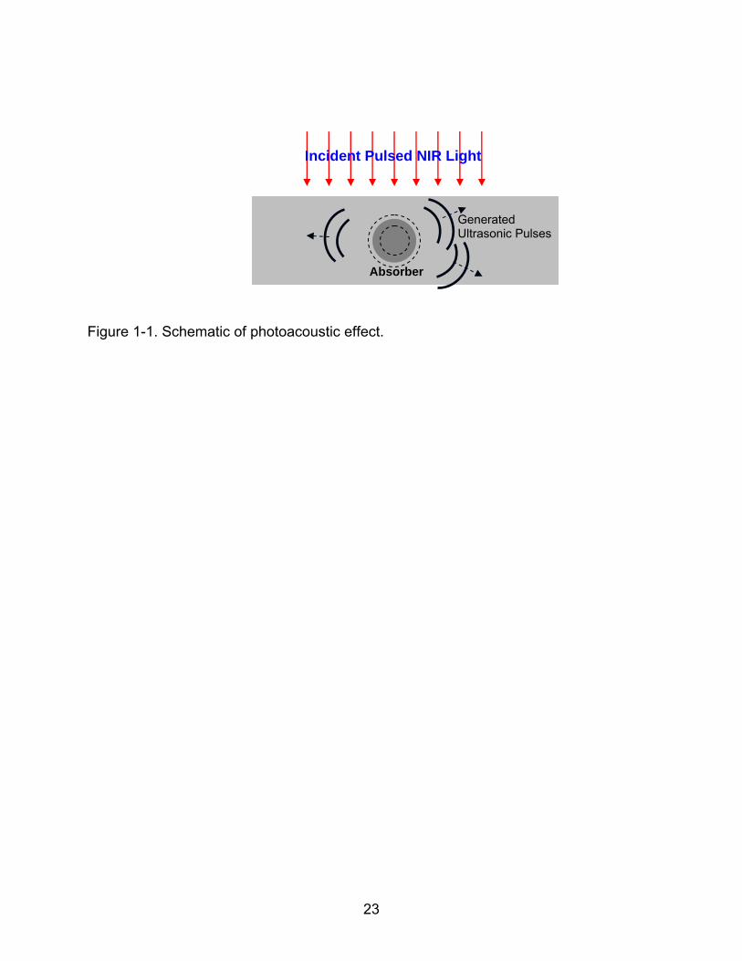
Photoacoustic tomography (PAT), also referred as optoacoustic tomography

(OAT), is an emerging non-ionizing and non-invasive imaging modality in the field of

biomedical imaging based on the physical principal of photoacoustic effect, where light

energy is converted into acoustic energy due to optical absorption and localized thermal

expansion in biological tissues as shown in the schematic of photoacoustic effect in

Figure 1-1. In photoacoustic tomography in biomedicine, pulsed laser beam with

duration in nanoseconds is delivered into biological tissues, and some of the delivered

energy will be absorbed and converted into heat, leading to transient thermoelastic

expansion and thus wideband ultrasonic emission. The generated ultrasonic waves

(~MHz) are then detected by ultrasonic transducers to form images.

As a hybridized imaging technique between optical imaging modality and

ultrasound imaging modality, PAT combines both high optical contrast and high

ultrasound resolution in a single modality. Studies have shown that optical absorption

contrast between tumor and normal tissues in the breast can be as high as 3:1 in near-

infrared region due to the significantly increased vascularity in the tumors.1-3 Significant

absorption contrast between diseased and normal joints has also been observed in the

hand with osteoarthritis (OA) and rheumatoid arthritis (RA).4-7 For example, for an

osteoarthritic joint, the ratio of its cartilage absorption coefficient to that of the

associated bone is increased by 40% relative to the healthy joints. Unfortunately, the

high optical contrast in biological tissues was poorly imaged in the pure optical imaging

methodologies, since optical scattering in soft tissues degrades spatial resolution

17

significantly with depth. For example, for imaging depth greater than ~1mm, the spatial

resolution provided by optical diffusion tomography is no better than 3mm. With PAT

technique, the high optical absorption contrast in biological tissues is recovered by

measuring the megahertz acoustic pressure wave with ultrasound detectors. Since

ultrasound scattering is two to three orders of magnitude weaker than optical scattering

in biological tissues, photoacoustic tomography is capable of providing significantly

improved yet depth-independent spatial resolution over all-optical imaging techniques

such as diffusion optical tomography (DOT).

Thus far, PAT has shown its potential to detect breast cancer, to assess vascular

and skin diseases, to monitor epilepsy in small animals, to image finger joints, to sound

out fluorescent proteins, and to evaluate exogenous contrast agents in molecular

imaging.8-24 Recent studies further demonstrated the possibility for PAT to image hard

tissues such as bones and associated soft tissues.25-27 In these studies, rat tail joint or

cadaver human finger joints were imaged and gold nanoparticles were used as contrast

agent to help diagnose / monitor RA disease.

While simplified 2-D PAT detection geometries and reconstruction algorithms have

been used in most of the previous studies, light scattering and pressure wave

propagation in tissue is inherently 3-D, and 2-D approximation to a real 3-D problem (2-

D reconstruction model with 2-D detecting geometry surrounding 3-D targets) will

inevitably bring errors, blurring and missing structures in the reconstructed 2-D images.

Besides that, the structures of the examined biological tissues remain unidentified in

sections other than the detecting plane, which may be important in some biomedicine

cases. For example, a finger joint from a human subject is highly irregular in its

18

volumetric structure. Although it seemed that tissues around proximal interphalangeal

(PIP) and distal interphalangeal (DIP) joints were well differentiated in reported 2-D

cross-sectional images of a photoacoustically examined cadaver human finger 25, some

tissue structures shown in the obtained 2-D cross sectional images were not in

agreement with those from histological photographs due to the collapse of the signals

from the entire 3-D joint structures into the 2-D cross-sectional imaging planes. While

RA disease can be diagnosed from the cross section images alone, it is known that the

coronal and sagittal section images of the finger joints are necessary for OA diagnosis

which is impossible for 2-D PAT. Thus, full volumetric image reconstruction is essential

to capture the joint tissues completely and accurately for diagnosis of both OA and RA.

Although studies on conventional PAT have focused on obtaining high resolution

anatomical structure of biological tissues by imaging absorbed optical energy density

(i.e., the product of the intrinsic absorption coefficient and the external optical fluence or

photon density), PAT is also capable of providing the intrinsic absorption coefficient

distribution when a light transport model is combine with conventional PAT method.28-34

Moreover, physiological / functional information such as oxygen saturation or the

concentration of hemoglobin, to which optical absorption is very sensitive, can also be

effectively recovered in high resolution when multispectral light is used.35-42 These

intrinsic tissue properties may be important for accurate diagnostic decision-making in

early stage of diseases.

1.2 Overview of Osteoarthritis

Osteoarthritis (OA) is the most common degenerative joint disease, affecting tens

of millions of Americans and involves over 500,000 individuals for joint replacement

annually in the United States.43-44

19

Primary OA commonly affects small joints in the hand, including the distal

interphalangeal (DIP) joints and the proximal interphalangeal (PIP), and large weight-

bearing joints in the hips and knees. Although knee and hip OA bear most responsibility

for the burden of OA, hand OA may be a marker of a systemic predisposition toward

OA; incidence study of OA further revealed that the second DIP joint is most frequently

affected (57% in women, 37% in men) among all the joints in the hand.45

Pain, stiffness, tenderness, joint enlargement and limitation of motion are the

typical symptoms and signs of OA, and the pathological features of OA include erosion

of articular cartilage and associated bony changes.46 Synovial effusion and associated

enhanced blood vessel growth may be occasionally observed as well in OA joints,

although it may not be as severe as that in joints affected by rheumatoid arthritis (RA).

Thus far, clinical examination remains the principal approach to OA diagnosis,

relying on symptoms and signs OA patients suffered as well as experience of arthritis

physicians. Imaging techniques, including standard x-ray radiography, computed

tomography (CT), ultrasonography and magnetic resonance imaging (MRI), have been

conventionally used or investigated to visualize the physiologic/anatomic abnormalities

in the joint cavity when OA has been established.47-54 However, all these available

imaging techniques are used only as supplemental methods in OA diagnosis, especially

in hand OA, either because they are insensitive to the abnormal changes in the OA joint

cavity or because they are too costly to be used as a routine examination method. For

example, plain radiographs are able to visualize structural abnormality in the bone

compartment (joint space narrowing and osteophyte formation) in joint cavity with high

spatial resolution when OA has been well established, however they are insensitive to

20

changes in soft tissues (cartilage, synovial fluid, etc) and therefore incapable of

capturing the primary features when OA is establishing in earlier stage.

As such, sensitive and affordable imaging methods are urgently needed for the

detection of OA, especially in early stages. Moreover, the progress of effective imaging

methods in OA diagnosis may at the same time accelerate the advancement of medical

therapies for OA, which are currently effective to relieve OA symptoms or prevent the

worsening of OA to a certain degree and yet of limited effectiveness in modifying OA.

Up to now, no disease-modifying OA drugs (DMOADs) has been approved. The

development of the DMOADs may benefit greatly from the progress of imaging methods

in OA diagnosis, where sensitive imaging techniques can serve as surrogate markers

for clinically meaningful outcomes to economically and efficiently validate the candidate

DMOADs.43

New imaging techniques based on near-infrared (NIR) light, including pure-optical

imaging techniques and photoacoustic tomography (PAT), have been recently studied

to image finger joints and to effectively detect joint diseases. 4-7,25, 55 The high “color”

contrast (absorption coefficient) provided by diseased biological tissues (as high as 3:1

between tumor and normal tissues; > 40% increase in absorption for osteoarthritic

cartilage compared to normal cartilage), has made NIR based imaging techniques a

promising modality for early disease detection.2-3 While optical imaging techniques are

able to detect the highly sensitive optical absorption / scattering abnormalities

associated with soft tissues (cartilage, synovial fluid, etc) in OA and RA joints, its spatial

resolution is relatively low (about 3~5mm). Compared to all-optical imaging techniques,

PAT is able to visualize the same optical absorption contrast with significantly improved

21

spatial resolution (0.5mm or better, adjustable with ultrasound frequency) for deep-

tissue imaging. For example, tendon, aponeurosis, volar plate, subcutaneous tissue,

phalanx and other tissues around DIP joints were well differentiated in high resolution

when a cadaver human finger was photoacoustically scanned in cross section with a

10MHz transducer.

In this study, we develop a full 3-D PAT approach (high performance 3-D PAT

reconstruction algorithm and a 3-D PAT system in spherical scanning geometry), aiming

to study finger joints imaging and detect osteoarthritis disease in the hand. The high

performance 3-D PAT reconstruction algorithm is based on parallel computing

technique and the finite element method, which is validated phantom experiments. The

feasibility, the optimal detector performance, and the optimal scanning geometry for 3-D

photoacoustic finger joints imaging were pre-investigated with a series of finger-joint

phantom experiments.56 A 3-D PAT system in a spherical scanning geometry has then

been constructed and optimized for in-vivo examination of human finger joints, and the

distal interphalangeal (DIP) joint from a human volunteer was imaged.57 The

performance of the 3-D PAT system has been further improved with an ultrasound

detection array composed of eight 1 MHz PZT transducers and a 16-channel

pulse/receive PCI board. The 3-D PAT system with eight detecting channels was

carefully calibrated with controlled tissue phantom experiments, and is capable of

completing a finger joint examination within 5 minutes (at single optical wavelength).

Seven subjects (two OA patients and five healthy controls) enrolled in our study from

2008 to 2009 were photoacoustically examined with our 8-channel 3-D PAT system.58

Major chromophore concentrations (HbO2, Hb) of in-vivo finger joints were further

22

quantitatively imaged by using multispectral 3-D PAT approach with six optical

wavelengths from 730nm to 880nm.59

23

Figure 1-1. Schematic of photoacoustic effect.

Incident Pulsed NIR Light

Absorber

Generated Ultrasonic Pulses

24

CHAPTER 2 RECONSTRCUTION ALGORITHM IN PAT

Thus far, several algorithms have been implemented to effectively reconstruct

photoacoustic images from measured acoustic waves, such as backprojection, Fourier

transform, P-transform, k-wave method and statistical approaches.60-64 While others rely

on analytical solutions to the photoacoustic wave equation in a regularly shaped

imaging domain and assume acoustical homogeneity in biological media, finite element

based algorithm seems provide unrivaled advantage to accommodate tissue

heterogeneity and geometric irregularity as well as allow complex boundary conditions

and source representations.65-67 Moreover, acoustic property in the biological tissues is

able to be recovered simultaneously with optical property by finite element based

algorithm, when acoustic heterogeneity is taken in consideration in photoacoustic wave

equation. In the following section, we will introduce the finite element based algorithm in

photoacoustic tomography in detail.

2.1 Finite Element Based Reconstruction Algorithm in PAT

For pulse mode PA generation propagating in soft tissues at room temperature,

the thermal diffusion and electrostrictive effects can be ignored. Therefore, only

considering the thermal expansion mechanism, the acoustic field by the PA generation

in tissue is described by the following wave equation:

22

2 2

1( , ) ( , )

P

p r t H r tc t C t

(2.1)

Where c is the speed of acoustic wave in the tissue; ( , )p r t

is the acoustic pressure;

is the thermal expansion coefficient; Cp is the specific heat at constant pressure; and

25

( , )H r t

is the heating function defined as thermal energy per time and volume absorbed

in the tissue.

Assuming the laser light is a delta function in time and uniformly irradiated on the

surface of the tissue, and the heating function ( , )H r t

can be written as the product of

spatial absorption function ( )r

and the temporal illumination as the form of delta

function ( )t , we can write equation (2.1) as

)()(),(1

2

2

22 tr

tCtrp

tc P

(2.2)

Taking the Fourier transform of the above equation (2.2) in the temporal domain,

we have the following Helmholtz equation:

2 2 ( )( , ) ( , )

p

c rP r k P r ik

C

(2.3)

Where k is the acoustic wave number defined as /k c , 2 f .

Although the acoustic speed c can be considered as a constant if we assume the

biological tissues are acoustically homogenous, it is indeed a variable quality in realistic

biological tissues. For variable acoustic speed in biological tissues, we can re-write

equation (2.3) as the following equation, in a reference of a constant acoustic speed in a

coupling medium

2 20

( )( , ) (1 ) ( , )

p

c rP r k P r ik

C

(2.4)

Where 2 20 / ( ) 1c c r

Choose j as the set of basis functions, and then the weighted weak form of

equation (2.4) can be stated as:

26

2 20

( )(1 ) 0j jV V

p

c rP k P dV ik dV

C

(2.5)

Expanding ( , )P r and ( )r

as the sum of complex coefficients multiplied by the

basis functions:1

N

i iiP p

,

1

N

i ii

,

1

N

k ki

the finite element discretization

of equation (2.5) can be written as the following linear equations:

A p b (2.6)

Where 2

2 20 0 2

( ) ( )jij j i j i k k j i j iV V V

A dV k dV k dV ds

0

1

N

i i j iViP

cb ik dV

C

TNpppp ,,, 21

And the following absorbing boundary conditions have been applied:

2

2ˆ

PP n P

(2.7)

Where

0

200

/1

8/32/3

ki

kiik

;

0

20

/1

2/

ki

ki

and is the angular coordinate at a

radial position .

2.1.1 Forward Modeling in Acoustically Homogenous Media

Although the acoustic speed c is indeed a variable quality in realistic biological

tissues, we may assume that the biological tissues are acoustically homogenous for

simplicity in some cases and consider the acoustic speed as a constant in interested

biological tissues during the process of image reconstruction. In these cases, equations

(2.6) can be simplified as the following equations

27

A p b (2.8)

Where 2

20 2

( )jij j i j i j iV V

A k ds

0

1

N

i i j i ViP

cb ik

C

TNpppp ,,, 21

In photoacoustic tomography with the assumption of acoustical homogeneity in

biological tissues, equation (2.8) serves as the forward model to compute the spatial

variation of acoustic pressure wave (external observable) based on a given optical

property distribution, or to compute the updated acoustic pressure wave in space based

on a initial guess or iterative value of an optical property distribution in image

reconstruction.

2.1.2 Inverse Modeling and Nonlinear Optimization in PAT Reconstruction

In the inverse problem of PAT reconstruction, the optical absorption distribution

(ultrasound source term in ultrasound propagation equation) was estimated given the

governing photoacoustic equations, boundary conditions, and measurements of the

pressure wave on the detecting locations (external observable). Gauss-Newton iterative

scheme combined with Marquardt and Tikhonov regularizations has been pursued in

our research to obtain stable inverse solution to the PA equation. This approach uses

the hybrid regularizations-based method to update an initial (guess) optical absorption

distribution iteratively to minimize an objective function composed of a weighted sum of

the squared difference between computed and measured data for all frequencies.

Unlike forward problem in PAT where the stiffness matrix A is well-conditioned and

the solution is well-defined, inverse problem in PAT has to estimate the spatial tissue

28

properties with limited observables on the boundary and most commonly results in ill-

posed situation, yielding meaningless solutions in image reconstruction. In ill-posed

situation, solutions in inverse problem may be non-unique, non-existent or unstable (a

tiny perturbation in the measurement results in large differences in the solution).68 To

improve the conditioning of the problem and enable a numerical solution in inverse

modeling, Tikhonov regularization was used to find an optimized solution in inverse

problem by minimizing the following modified objective function

2 2( ) ( )c mF p p

(2.9)

Where the second term is an added penalizing factor with a weighting in a Euclidean

distance referenced to , and is set equal to the parameter distribution at the

previous iteration ( )i for simplicity in Levenberg-Marquardt algorithm.

At the thi iteration, we assume that the Taylor’s expansion of the objective function

( )F around ( )i can be expressed as

( )( ) ( ) ( ) ( ) 2( )

( ) ( ) ( )( ) ( )2

ii i i iFH

F F F

(2.10)

Where ( )( )iF

and ( )( )iFH are the first and second order derivative

At the minimum of the objective function ( )F , we have stationary point where the

following identity is satisfied

( )0

dF

d

(2.11)

Substituting (2.10) into (2.11) and ignoring the derivatives higher than second

order, we have the following Gauss-Newton iterative scheme

1( 1) ( ) ( ) ( )( ) ( )i i i iFH F

(2.12)

29

Consider the regularized objective function given in equation (2.9), where ( )i

,

we have the first and second order derivative of the objective function ( )F

( )( )( ) 2 ( ) 2 ( )

cc m idp

F p pd

( ) ( )( ) 2 2

c c

F

dp dpH

d d

(2.13)

Combining the above first and second order derivative of the objective

function ( )F with the Gauss-Newton iterative scheme (2.12), we have the iterative

equation

( 2 ) ( )T m cJ J J T I χ p p

(2.14)

Where the Jacobian matrix J is defined over total M detecting locations as

1 1 1

1 2

2 2 2

1 2

1 2

N

N

M M M

N

p p p

p p p

J

p p p

1 2, , ,Tc c c c

Mp p p p

1 2, , ,Tm m m m

Mp p p p

( 1) ( )1 2, , ,

Ti iN χ χ χ

(2.15)

Since p

is a linear function of from the linear equation set (2.8), we can calculate

jkJ by applying partial differentiation on equation (2.8) with respect to k ,

30

( ) ( )ij j ij j

k k

A p B

, 0

ij jS iP

cB ik dS

C

(2.16)

ijA and ijB are independent on k , and j k ij since j and k are independent

variable if j k , therefore we have

ij jk ij jk ikA J B B (2.17)

In photoacoustic tomography, the final equation (2.14) with Jacobian matrix

determined in equation (2.17) is the core of the inverse computation to update the

optical property distribution from an initial estimate. In each iterative step, it compares

the measured with the solved observables, which is the acoustic pressure wave for

different frequencies obtained via the forward model (2.8) and current estimate of the

optical property distribution, and solves the inverse problem by nonlinear optimization

equation (2.14) to obtain a new estimate of the optical property distribution. This

procedure is iteratively repeated until optimal least-squares fit of computed and

measured acoustic data is reached.

2.1.3 Regularization in PAT Reconstruction

The purpose of introducing the Tikhonov regularization on the Hessian matrix H is

to ensure the diagonal dominance and enable a stable numerical solution in inverse

procedure. However, the optimal weighting factor is problem-specific and sometime

quite difficult to determine. An effective approach for choosing optimal weighting

factor is to iteratively modify its value based on the trace of the Hessian matrix and the

relative least-square error rele at each iterative step: 69

([ ])Trele trace J J (2.18)

Where is an empirical coefficient. We normally use 0.5 in our PAT problem.

31

Since the weighting factor relies on rele which iteratively decreases, the value of

and the regularization effect will be reduced at each iterative step. The variation of

in each step allows more accurate image to be revealed as the iterations progress,

while a blurred image is initially reconstructed with large at the start of the iterations.

The empirical coefficient is carefully chosen so that the image can be accurately

reconstructed with iterations while stability to a numerical solution is ensured at the

same time.

Although weighting factor defined as identify (2.18) in Tikhonov regularization

enable the stable numerical solution in inverse problem, the Gauss-Newton iterative

scheme may experience problem in iterative convergence since the approximation

(2.10) of Gauss-Newton iterative scheme are iteratively valid only near the minimum

(actual solution). If the initial estimates are far from the actual solution, Gauss-Newton

iterative scheme may have difficulty in convergence.

Other than Gauss-Newton iterative scheme, gradient descent, also referred as

steepest descent, relies barely on the initial estimates although it may exhibit oscillation

around the minimum and the convergent process is slow,68 since the first order

derivative of objective function is used in gradient descent instead of second order

derivative used in Gauss-Newton iterative scheme. The real-valued objective function

( )F decreases fastest from a given estimate along the direction of the negative

gradient of ( )F at the given estimate, and hence the iterative algorithm for gradient

descent is given by

( 1) ( 1) ( ) ( )( )i i i iF

(2.19)

Where ( )i is a positive value used as iterative step size.

32

Considering ( )( )iF

given by equation (2.13) from Tikhonov regularized objective

function (2.9), we have the following iterative algorithm for gradient descent

1( ) ( )2

T m cJ χ p p

(2.20)

Comparing the gradient descent method given in (2.20) and the Gauss-Newton

iterative scheme given in (2.14), we may see some similarity between them. With a

hybrid technique proposed in Levenberg-Marquardt method, we can use a steering

factor to switch between the Gauss-Newton iterative scheme and gradient descent

method. The final update equation can be written as

( ) ( )T m cJ J J T I I χ p p

(2.21)

Where is a weighting factor used in Tikhonov regularization to relieve the ill-posedness

of the inverse problem; is a steering factor introduced in Levenberg-Marquardt

method to balance the convergent ability and the convergent speed.

When the steering factor is very big, the term J JT can be ignored and equation

(2.21) shows the iterative behavior of gradient descent method shown in equation

(2.20). When is small, then equation (2.21) reduces to equation (2.14) and exhibits

the behavior of Gauss-Newton iterative scheme. So practically, the value of is

chosen iteratively by the following rules:

1) The steering factor is initially set with a big value so that the initial estimates

can be chosen with less caution with the gradient descent behavior shown in (2.21).

2) In each iterative step, the steering factor reduces by a given ratio (such as

10) to accelerate the convergence process if the objective function decreases.

Otherwise, the steering factor is increased by a given ratio.

33

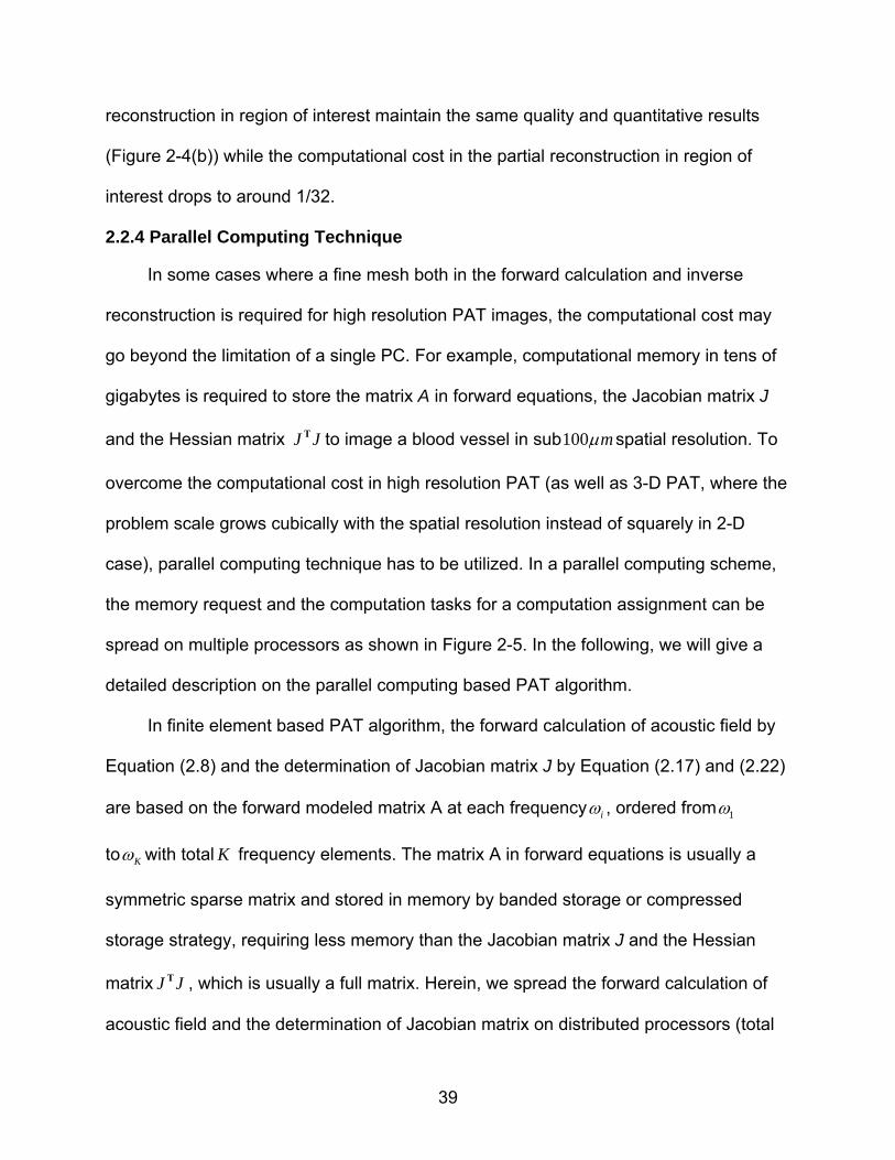
2.1.4 Simulation in PAT Reconstruction

The reconstruction algorithm developed for 3-D PAT is tested with simulated finger

joints, where a cylindrically simulated finger with a 2.5mm thickness “cartilage”

sandwiched between two bones is buried in background. The absorbed energy contrast

between the simulated cartilage and the bones is assumed as 3:1, and the two bones

are 10mm in diameter.

The mesh for algorithm testing is a cylindrical mesh with total 14784 tetrahedral

elements and 2907 nodes, which is generated from a 2-D triangle mesh slice layer by

layer. Each layer of the total 17 layered cylindrical mesh has 308 elements and 171

nodes, with layer interval 1.25mm in the axial direction (Z axis). The coronal section and

the cross section of the reconstructed finger joint from simulated data are shown in

Figure 2-1, where the actual shape of the simulated finger joint is outlined with black

dash lines. From the reconstructed finger joint, we can see the bones and the cartilage

are recovered with great quality. The structure and the size of the bones and the

cartilage are in great agreement with the actual shape and size of the simulated bones

and the cartilage. And the absorbed energy contrast between the simulated cartilage

and the bones is also recovered with high accuracy. The results shown in this

simulation validate the reconstruction algorithm of 3-D PAT for further finger joint

imaging.

2.2 Computing Strategies in PAT Reconstruction

In finite element based PAT reconstruction, the major task is solving the forward

equations (2.8), the Jacobian matrix (2.17) and the inverse equations (2.14), which are

normally time / memory costly depending on the scales of the linear system of equation

(the total number N of finite element nodes). As the scale increase, the cost in

34

computational memory and time grows dramatically, which may go beyond the

computation limitation of a single PC. Herein, some efficient computing strategies have

been adopted to bring the high resolution PAT in full potential.

2.2.1 Adjoin Sensitivity Method

Normally only the pressure on the boundary nodes (total M nodes) is observable,

therefore, in the calculation of jkJ , only det( ), 1, 2, ,j s s M is useful for updating

in

the inverse equation (2.14). Considering the Jacobian matrix defined in equation (2.17),

we have

1

, ,sk s j jk s j ij ik si ikJ J A B S B

(2.22)

Where ,s j is defined as , 1s j for det( )j s , otherwise , 0s j ; and siS can be

calculated from ,s j si ijS A

It is worth to note that 0ikB if node i and k belong to different element as

shown in equation (2.16). As a result, we only need sum up the contribution of the

nodes in elements contain node k , even though the sum index i in siS varies from 1

to N .

2.2.2 Dual Meshing Scheme

In finite element based reconstruction algorithm, spatial sampling rate (mesh

density) that is used to discretize the target region is critical and greatly determines the

computational costs and the resolution of the reconstructed images. For example, the

rapid spatial variation in the field of acoustic pressure wave (megahertz frequencies)

governed by the photoacoustic wave equation demands high mesh resolution

(typically /10 , is the ultrasound wavelength) with finely discretized mesh in order to

35

maintain forward calculation accuracy of the acoustic pressure field in the media.

However a finely discretized mesh with increased spatial sampling rate, and hence the

total numbers of mesh nodes, will inevitably results in dramatically growing

computational cost, which almost grows squarely and cubically with the total mesh

number in the forward calculation of the acoustic pressure and the inverse image

reconstruction of unknown absorbed energy profiles (or absorption coefficient profiles),

respectively. At the same time, the unknown absorbed energy profiles to be

reconstructed in PAT are relatively uniform and hence representable with fewer mesh

nodes (degrees-of-freedom). To balance the accuracy required for the calculation of the

acoustic pressure wave and the cost of computation, dual-mesh scheme seems an

optimal solution in the finite element based PAT algorithm, where a dense mesh is used

in the forward calculation of the acoustic pressure and a relatively coarse mesh is used

in the inverse image reconstruction. 71

Implementation of the dual mesh scheme affects two components of the

reconstruction algorithm:71-73 (1) the forward calculation of the acoustic pressure field in

the media at each iteration, where the updated absorbed energy profile to be used in

the forward calculation is defined on the coarse mesh while the forward calculation is

based on the fine mesh, and (2) calculation of the Jacobian matrix that is used to

update the estimates of the absorbed energy profile during the inverse image

reconstruction.

To calculate the acoustic pressure field in the media with the updated absorbed

energy defined on the coarse mesh, interpolation process is required to get the

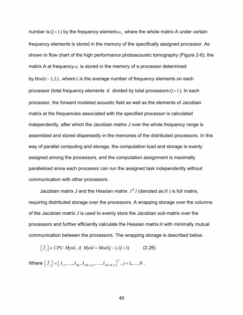
absorbed energy profile over the fine mesh from the coarse mesh. Assume that the thi

36

fine mesh node is inside the coarse mesh L , as shown in Figure 2-2(a) for a simplified

2-D case and Figure 2-2(b) for a 3-D case, the absorption energy value i at the thi fine

mesh node can be interpolated by the following formula

1

( )p

n n

N

i L L in

r

(2.23)

Where nL is the absorbed energy value at each node of the coarse mesh L , pN is the

number of the element nodes. 3pN for 2-D triangle mesh, and 4pN for 3-D

tetrahedral mesh.

For a certain pair of coarse/fine mesh, the interpolation coefficient ( )nL ir

is

always a constant, and therefore can be pre-calculated and stored in a mesh related file

before the reconstruction process, which saves the time of re-computing during each

iteration step.

With the dual mesh scheme, the elements of the Jacobian matrix will be calculated

by

0, jij ik ik kS i

k P

p cA B B ik dS

C

(2.24)

Where k is the node on the coarse mesh, k is the basis function centered on node k in

this mesh, and the integration is still performed over the elements in the fine mesh.

Since k and i are the basis functions defined over the coarse mesh and fine mesh,

respectively, the integration kernel k i is non zero only in the overlapping zone of the

coarse mesh the coarse node k belongs to, and the fine mesh the fine node i belongs

to. Complications arise from the integration when the fine mesh spans more than one

coarse element. To simplifying this problem, we can generate the fine mesh from the

37

coarse mesh by splitting the coarse elements into fine elements so that each fine mesh

resides entirely within one coarse mesh element as shown in Figure 2-2(c).

2.2.3 Partial Reconstruction in Region of Interest

Unlike optical tomography which is an inverse field problem to quantitatively

reverse the optical scattering / absorption properties in the media by measuring the

transported light arriving optical detectors from light sources, photoacoustic tomography

is indeed an inverse source problem. In photoacoustic tomography, the goal is to trace

the ultrasound sources (optical absorbers excited by near-infrared pulse) by measuring

the ultrasound field on a boundary with pre-known ultrasound properties in the media.

The particular feature of this imaging technique gives us an inspiration that we may

confine our inverse reconstruction in the region of interest that may contain the

ultrasound sources, which could greatly reduce the computation cost in the inverse

procedure.

To confine our inverse reconstruction in the region of interest, a slight adjustment

on the inverse equation is required where inverse Equation (2.14) is rewritten as

( 2 ) ( )T m cJ J J T I χ p p (2.25)

Where the new Jacobian matrix J is defined as

1 1 1

1 2

2 2 2

1 2

1 2

K

K

M M M

K

p p p

p p p

J

p p p

38

The new Jacobian matrix J is therefore a first order derivative of the ultrasound

pressure at each detecting location to the unknown optical absorbed energy (the

intensities of ultrasound sources) at each finite element node within the region of

interest, which includes total K finite element nodes.

The partial reconstruction is tested by simulation, where a cylindrical target (10mm

in diameter with 20mm height) is embedded in a cylindrical background. The contrast

between the target and the background is 7:1. The section image along the axis of the

cylindrical target from the reconstructed 3-D images with full volume reconstruction is

shown in Figure 2-3(a), where total 2907 nodes in the whole volume are involved in the

inverse reconstruction. At the same time, the cylindrical target is reconstructed with

partial reconstruction in region of interest, which is a small cylindrical volume containing

the cylindrical target. The region of interest include total 801 nodes and is outlined with

dash black lines in the section image along the axis of the cylindrical target as shown in

Figure 2-3(b), which is a 2-D section image from the reconstructed 3-D images with

partial reconstruction in the region of interest. As observed from Figure 2-3(b), the

partial reconstruction in region of interest in our study obtained almost the same image

shown in Figure 2-3(a) with full volume reconstruction in term of structure and

quantitative values, while the computational cost in the partial reconstruction in region of

interest is only around 1/47 of the computational cost in full volume reconstruction.

The partial reconstruction is further validated with phantom experiment as shown

in Figure 2-4, where the full volume contains 1301 nodes and the region of interest

outlined with black dash line includes only 229 nodes. Compared with the reconstructed

images with full volume reconstruction (Figure 2-4(a)), images reconstructed with partial

39

reconstruction in region of interest maintain the same quality and quantitative results

(Figure 2-4(b)) while the computational cost in the partial reconstruction in region of

interest drops to around 1/32.

2.2.4 Parallel Computing Technique

In some cases where a fine mesh both in the forward calculation and inverse

reconstruction is required for high resolution PAT images, the computational cost may

go beyond the limitation of a single PC. For example, computational memory in tens of

gigabytes is required to store the matrix A in forward equations, the Jacobian matrix J

and the Hessian matrix J JT to image a blood vessel in sub100 m spatial resolution. To

overcome the computational cost in high resolution PAT (as well as 3-D PAT, where the

problem scale grows cubically with the spatial resolution instead of squarely in 2-D

case), parallel computing technique has to be utilized. In a parallel computing scheme,

the memory request and the computation tasks for a computation assignment can be

spread on multiple processors as shown in Figure 2-5. In the following, we will give a

detailed description on the parallel computing based PAT algorithm.

In finite element based PAT algorithm, the forward calculation of acoustic field by

Equation (2.8) and the determination of Jacobian matrix J by Equation (2.17) and (2.22)

are based on the forward modeled matrix A at each frequency i , ordered from 1

to K with total K frequency elements. The matrix A in forward equations is usually a

symmetric sparse matrix and stored in memory by banded storage or compressed

storage strategy, requiring less memory than the Jacobian matrix J and the Hessian

matrix J JT , which is usually a full matrix. Herein, we spread the forward calculation of

acoustic field and the determination of Jacobian matrix on distributed processors (total

40

number is 1Q ) by the frequency element i , where the whole matrix A under certain

frequency elements is stored in the memory of the specifically assigned processor. As

shown in flow chart of the high performance photoacoustic tomography (Figure 2-6), the

matrix A at frequency i is stored in the memory of a processor determined

by ( 1, )Mod i L , where L is the average number of frequency elements on each

processor (total frequency elements K divided by total processors 1Q ). In each

processor, the forward modeled acoustic field as well as the elements of Jacobian

matrix at the frequencies associated with the specified processor is calculated

independently, after which the Jacobian matrix J over the whole frequency range is

assembled and stored dispersedly in the memories of the distributed processors. In this

way of parallel computing and storage, the computation load and storage is evenly

assigned among the processors, and the computation assignment is maximally

parallelized since each processor can run the assigned task independently without

communication with other processors.

Jacobian matrix J and the Hessian matrix J JT (denoted as H ) is full matrix,

requiring distributed storage over the processors. A wrapping storage over the columns

of the Jacobian matrix J is used to evenly store the Jacobian sub-matrix over the

processors and further efficiently calculate the Hessian matrix H with minimally mutual

communication between the processors. The wrapping storage is described below.

, ( 1, 1)jJ CPU Myid if Myid Mod j Q

(2.26)

Where 1 ( 1) ( ), , , , , , 1, ,T

j j Mj M j M K jJ J J J J j N

.

41

With the wrapping storage of the Jacobian matrix J, the Hessian matrix H can be

calculated and stored by

1 2 , ( 1, 1)T

j j jH J J J J CPU Myid if Myid Mod j Q

(2.27)

Where 1 , , , 1, ,T

j j jjH H H j N

.

Because the Hessian matrix H is symmetric, we store only the upper triangle of the

Hessian matrix spread over the processors. In the calculation of element ijH ,

communication and data exchange may be involved among the distributed processors,

except that the vector jJ

and jJ

are both stored in the memory of the same

processor. Since the Hessian matrix is stored dispersedly, the inverse reconstruction

by Equation (2.14) requires a parallel solving method, where parallelized Cholesky

decomposition is used in our high performance PAT.

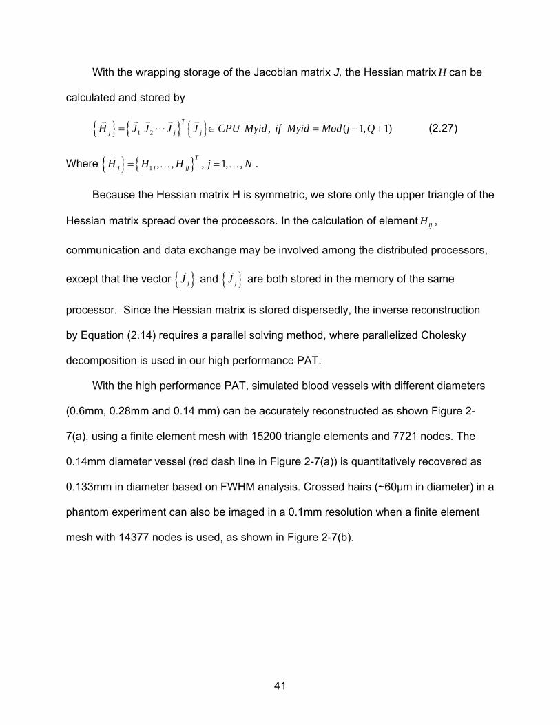
With the high performance PAT, simulated blood vessels with different diameters

(0.6mm, 0.28mm and 0.14 mm) can be accurately reconstructed as shown Figure 2-

7(a), using a finite element mesh with 15200 triangle elements and 7721 nodes. The

0.14mm diameter vessel (red dash line in Figure 2-7(a)) is quantitatively recovered as

0.133mm in diameter based on FWHM analysis. Crossed hairs (~60μm in diameter) in a

phantom experiment can also be imaged in a 0.1mm resolution when a finite element

mesh with 14377 nodes is used, as shown in Figure 2-7(b).

42

(a)

(b) Figure 2-1. The reconstructed images for simulated finger joint (a) coronal section slice

along X=0mm (b) cross section slice along Z=15mm.

(a)

(b)

(c)

Figure 2-2. Geometry of the absorbed energy interpolation at fine node i in 2-D case (a)

and in 3-D case (b), and the calculation of the Jacobian matrix element in the effective integration zone (c).

i

L1

L2

L3 L4

43

(a)

(b)

Figure 2-3. Slice along the axis of the cylindrical target from reconstructed 3-D images with full volume reconstruction (a), and partial reconstruction in region of interest (b).

(a)

(b)

Figure 2-4. Reconstructed 2-D images of a circular target in a phantom experiment with full volume reconstruction (a), and partial reconstruction in region of interest (b).

44

Figure 2-5. Schematic of parallel computing with a combination of both shared memory and distributed memory.

…CPU CPU

CPU CPU

Memory

CPU CPU

CPU CPU

Memory

CPU CPU

CPU CPU

Memory

CPU CPU

CPU CPU

Memory

…

A Computation Assignment

45

Figure 2-6. Flow chart of the high performance photoacoustic tomography based on parallel computing technique and finite element method.

( 1 ~ )i i Q L K ( 1 ~ 2 )i i L L

( )r initial values

( 1 ~ )i i L

Solving p by

A p b

,

1 ~ , 1 ~

si

s j si ij

Solving S by

S A

s M i N

Solving p by

A p b

Solving p by

A p b

,

1 ~ , 1 ~

si

s j si ij

Solving S by

S A

s M i N

CPU 0 CPU 1 CPU Q

Fill sub-matrix 0J Fill sub-matrix 1J Fill sub-matrix QJ

CPU communication and organize sub-matrix ( 0 ~ )iJ i Q

Calculate error function ( ) ( )( ) ( )c me p r p r

Is error small enough?

Stop Yes

No

CPU communication and Fill Hessian sub-matrix

Solve the inverse equations in parallel and update ( )r

,

1 ~ , 1 ~

si

s j si ij

Solving S by

S A

s M i N

46

(a)

(b)

Figure 2-7. The reconstructed images for simulated blood vessels (a) and crossed hairs in phantom experiment (b).

47

CHAPTER 3 PRE-INVESTIGATION OF 3-D PAT SYSTEM WITH TISSUE PHANTOM STUDY

In this section, we aim to systematically evaluate the possibility of 3-D

photoacoustic imaging of the finger joints, based on a series of tissue-like phantom

experiments. The 3-D structures and absorption coefficient images of the joint-

mimicking phantoms are obtained using finite element based PAT reconstruction

algorithm and its enhancement.

Among different 3-D scanning geometries, cylindrical scanning geometries (shown

in Figure 3-1) adopted from DOT seem straightforward and are easiest to implement,

however they give poor resolution along the cylindrical axis due to the limited aperture

size of a transducer. For example, a joint-like phantom with cartilage thickness in 1mm

was scanned by a 1MHz transducer in a cylindrical scanning geometry shown in Figure

3-1(a), and the joint space is missing in the reconstructed images as shown in Figure 3-

2. A transducer with small aperture size can theoretically offer enhanced resolution;

however, such a transducer often gives poor signal-to-noise ratio (SNR) with added

cost. Compared to a cylindrical scanning geometry, a spherical scanning geometry with

a modest size of transducer aperture may provide an optimal solution for 3-D imaging

as the spatial resolution with such a scanning depends little on the aperture size of the

transducer, especially around the center of the imaging zone. In this study, phantom

experiments based on both cylindrical scanning geometry and spherical scanning

geometry are conducted for comparison, the results of which show that spherical

scanning geometry provides obvious spatial resolution improvement over cylindrical

scanning geometry and might be suitable for finger joint imaging. The spherical

scanning geometry is adopted in further phantom experiments to systematically

48

evaluate the differentiability in controlled phantoms with varied thickness and varied

optical absorption values in “cartilage”.

3.1 Tissue Mimicking Phantom

To evaluate the reconstruction algorithm of 3-D PAT and the possibility of 3-D

photoacoustic imaging of the finger joints with phantom experiments, solid tissue

phantoms that well approximate optical characters of in-vivo finger joints are fabricated.

The solid tissue phantoms used here are made of Intralipid, India ink, distilled water and

agar powder, among which Intralipid acts as the optical scatter, India ink supplies color

contrast (optical absorber) and the agar (1%-2%) serves as the coagulator. The joint-

like tissue phantoms used in our experiments are optically well-characterized, in term of

the optical absorption/scattering coefficients. The highly purified agar powder (A-7049,

Sigma, USA) is dissolved in distilled water, and is liquefied after being boiled to the

melting temperature of 95oC with a regular microwave oven. The solution has to be

stirred continuously in order to obtain good uniformity in fabricated phantom while

cooling down to 40oC, when the solution must be poured into a mould and left there for

some time (normally about 10 minutes for 400mL solution) to reach a proper hardening

and stable optical properties. The optimal temperature for adding Intralipid and India ink

to the agar solution is around 60oC, although it is non-critical between 80oC and 40oC.

The detailed fabrication procedure and the performance in controlled optical properties

of the tissue phantom have been fully described before.74

The two phantom “bones” fabricated in our study to mimick real finger bones had:

a = 0.07mm-1, s =2.5mm-1 and a diameter of 6mm, and the “cartilage” between the

bones had: a = 0.015~0.04mm-1, s =1.5mm-1 and a thickness of 1 or 2mm, as shown

49

in Table 3-1. All the optical properties of the fabricated phantom are based on real finger

joints.

3.2 System Description and Experiments

The joint-like tissue phantom experiments in this study were conducted with a 3-D

PAT imaging system as shown in Figure 3-3, which is capable to scan the phantoms

along a cylindrical surface as well as along an equivalent spherical surface.

The Ti: Sapphire laser (LOTIS, Minsk, Belarus) generates a pulsed beam with a

pulse repetition rate of 10 Hz and a pulse width <10ns. The wavelength of the laser was

tunable from 600 to 950nm and was locked at 820nm in our experiments for deep

medium penetration. After the reflection mirror, the laser is then expanded by a lens and

a ground glass so that the phantom can be uniformly illuminated by an area source of

light. The laser energy used at the phantom surface was about 10mJ/cm2, which is far

below the safety standard of 22mJ/cm2.

To detect the acoustic field generated by the pulsed laser, 1 MHz transducer

(Valpey Fisher, Hopkinton, MA) was used. The transducer has a bandwidth of 80% at -

6dB and an aperture size of 6mm. To reduce the attenuation of the acoustic field, the

transducer and the phantom were all immersed in a water tank, in which the sound

speed was specified as 1495m/s.

During an experiment, the phantom was placed at the center of the rotary stage,

and the transducer was attached to the rotary stage via an arm having a length of

~20mm. To acquire the acoustic field along a cylindrically scanning surface, the

transducer was stepped along the Z axis as well as rotated along an arc facing the

center of the joint-like phantom in XY plane. In our experiments, the arc scanning in the

XY plane covered 300º around the phantom as shown in Figure 3-4, allowing the

50

collection of signals at 50 locations with a step interval of 6º; the linear scanning along

the Z axis permitted data collection at 650 positions along the cylindrical surface using

13 steps with an interval of 1mm.

For the spherical scanning mode, the arc scanning in the XY plane covered the

same 300º around the phantom as the cylindrical scanning, and the phantom was also

rotated along the Y axis so that the transducer was equivalently rotated around the

phantom. The phantom was rotated 15º per step along the Y axis until a full spherical

surface was covered, which allowed the data collection at 600 scanning positions.

The detected acoustic signals were amplified and filtered by a Pulser/Receiver

5058PR (Panametrics, Waltham, MA). The bandwidth of 5058PR ranges from 10kHz to

10MHz, and five scales from 0.01 to 1.0MHz are selectable in high pass filtering. The

preamplifier integrated in 5058PR is in 30dB gain and the gain of the 5058PR itself is

40/60dB with attenuation tunable from 0dB to 80dB in 1dB steps. The Labview

programming was used to control the entire data acquisition procedure.

3.3 Methods

Our finite element based 3-D PAT reconstruction algorithm and its enhancement

for extracting quantitative absorption includes two steps. The first is to obtain the 3-D

images of absorbed optical energy density through our 3-D PAT reconstruction

algorithm that is based on finite element solution to the photoacoustic wave equation in

frequency domain subject to the radiation or absorbing boundary conditions (BCs),

which is described in detail in Chapter 2. The second step is to recover the optical

absorption coefficient distribution using the photon diffusion model coupled with the

absorbed optical energy density images obtained from the first step.

51

In the first step, the 3-D PAT reconstruction algorithm uses the regularized Newton

iterative strategy to update an initial absorbed optical energy density distribution to

minimize an object function, which is composed of a weighted sum of the squared

difference between computed and measured acoustic data.

To recover the optical absorption coefficient from absorbed energy density, , the

photon diffusion equation as well as the Robin boundary conditions can be written in

consideration of a ,

D( r ) E( r ) ( r ) ( r ) S( r ) (3.1)

( ) ( ) ( ) ( ) ( )D r E r r n E r r (3.2)

Where ( ) 1/ ( )aE r r , ( )D r

is the diffusion coefficient, ( ) 1/ 3( ( ) ( ))a sD r r r and ( )s r is

the reduced scattering coefficients, is a boundary condition coefficient related to the

internal reflection at the boundary, and S( r ) is the incident point or distributed source

term. For the inverse computation, the so-called Tikhonov-regularization sets up a

weighted term as well as a penalty term in order to minimize the squared differences

between computed and measured absorbed energy density values,

2 2

0( ) ( ) ( )[ ( ) ( )]c oMin r r r r r

Φ Φ L E E (3.3)

Where L is the regularization matrix or filter matrix, is the regularization parameter,

o o o o T1 2 N( , ,..., ) Φ and c c c c T

1 2 N( , ,..., ) Φ where oiΦ is the absorbed energy density

obtained from PAT, and ciΦ is the absorbed energy density computed from Equations.

(3.1) and (3.2), for i=1, 2…, N locations within the entire PAT reconstruction domain.

The initial estimate of absorption coefficient can be updated based on iterative Newton

method as follows with =1,

1( ) ( ) [ ( )]T T T o c E J J I L L J Φ Φ (3.4)

52

In addition to the usual Tikhonov regularization, the PAT image (absorbed optical

energy density) is used both as input data and as a priori structural information to

regularize the solution so that the ill-posedness associated with such inversion can be

reduced. The whole imaging zone is segmented by Amira (Indeed-Visual Concepts

GmbH, Berlin, Germany) into several sub-regions, and the segmented a priori spatial

information based on the PAT image can be incorporated into the iterative process

using Laplacian-type filter matrix, L ,

1

1/ ,

0 ,ij

if i j

L NN if i j one region

if i j diffrent region

(3.5)

Where NN is the total node number within one region or tissue; the optical absorption

coefficient distribution is then reconstructed through the iterative procedures described

by equation (3.1) and (3.3), where a priori spatial information from the PAT image is

incorporated in through the matrix L.

3.4 Results and Discussion

The 3-D images were reconstructed using a finite element mesh of 41323

tetrahedral elements and 7519 nodes which required around 120 minutes per iteration

for a total of 10 iterations on a computation cluster with 10 processors. Each of the

processors worked at 2.2GHz with 2GB memory.

The comparison between the cylindrical and spherical scanning geometries can be

made from the images shown in Figure 3-5a and Figure 3-5b for a typical joint-like

phantom with 1mm-thick cartilage. Figure 3-5a display the coronal, sagittal and cross

sections of the 3-D images from the reconstructed absorbed energy density distributions

with the cylindrical scanning, while Figure 3-5b show the corresponding sectional

images with the spherical scanning geometry. To compare the reconstructed images

53

with the phantom, the actual shape of the phantom is outlined in Figure 3-5 (Dashed

rectangular or circle). As can be observed from Figure 3-5a, the phantom structures in

the coronal section (XY plane) are well reconstructed, while both the structures in the

sagittal and cross sections (YZ and XZ planes) are clearly distorted especially for the

cross section. Here we see that the structures along the circular plane (XY plane) can

be recovered accurately and that the structures are erroneously stretched along the

cylindrical axis (Z axis). The images presented in Figure 3-5b with the spherical

scanning show clear improvement over that using the cylindrical scanning. We see that

there is almost no distortion along the Z axis especially for the cross section. These

images with the spherical scanning are quantitatively accurate in terms of the recovered

size, shape and location of the objects.

Since the spherical scanning gives us the best image quality for 3-D joint imaging,

the remaining results were all obtained based on this scanning geometry. Figure 3-5c

presents the coronal, sagittal and cross sections of the reconstructed 3-D absorbed

energy density for a joint-like phantom with 2mm-thick cartilage. It is observed from

Figure 3-5b and 3c that the structures along each section are well detected and that the

thickness of cartilage for both 1mm and 2mm cases are correctly recovered. The

recovered absorption coefficient images and their profiles along a transect in the sagittal

section are displayed in Figure 3-6 and 3-7, respectively. We see that the reconstructed

absorption coefficients of the bones and cartilage are quantitatively accurate relative to

their actual values. By estimating the full width at half maximum (FWHM) of the

absorption coefficient profiles, the recovered cartilage thickness was found to be

54

around 1.3 and 2.3mm, which are in good agreement with the actual object size of 1

and 2mm used in the experiments.

We also conducted experiments to evaluate the ability of resolving different optical

contrasts when the absorption coefficient of cartilage varied from 0.015 to 0.04 mm-1.

The reconstructed results from these experiments are shown in Figure 3-8, where

Figure 3-8a to 3-6d display the coronal, sagittal and cross sections of the reconstructed

3-D absorbed energy density when the cartilage had an absorption coefficient of 0.015

mm-1, 0.025 mm-1, 0.03mm-1 and 0.04 mm-1, respectively. We can observe that the

bones and cartilage are clearly distinguishable when the absorption contrast between

the bones and cartilage is large (Figure 3-8a and 3-8b) and that it is increasingly difficult

for these two types of structures to be separated (Figure 3-8c and 3-8d). The recovered

absorption coefficient images and their profiles along a transect in the sagittal section

are displayed in Figure 3-9 and Figure 3-10. We note that the absorption coefficient of

the cartilage is quantitatively recovered–it was found to be around 0.016, 0.026, 0.031

and 0.043 mm-1, which are in very good agreement with the actual values of 0.015,

0.025, 0.03 and 0.04 mm-1.

It is worth to note that homogeneous acoustic speed was assumed in this study

which is certainly an approximation to the possible heterogeneous acoustic medium

used in the experiments. Previous studies have shown that this assumption may

generate blurring in the reconstructed images. However, Compared to the blurring

effects from an inappropriate scanning geometry and detection configuration, the

blurring due to the assumption of homogeneous acoustic speed is significantly smaller,

especially for larger dimension targets. In addition, the blurring due to the assumption of

55

homogeneous acoustic speed can be eliminated by the use of advanced reconstruction

algorithms without such an assumption.

In summary, in this study we have shown that a spherical scanning geometry is

probably an optimal way for us to perform 3-D PAT imaging of the finger joints. Our

results also indicate that the joint-like structures and their absorption coefficients can be

quantitatively reconstructed using our 3-D PAT approach.

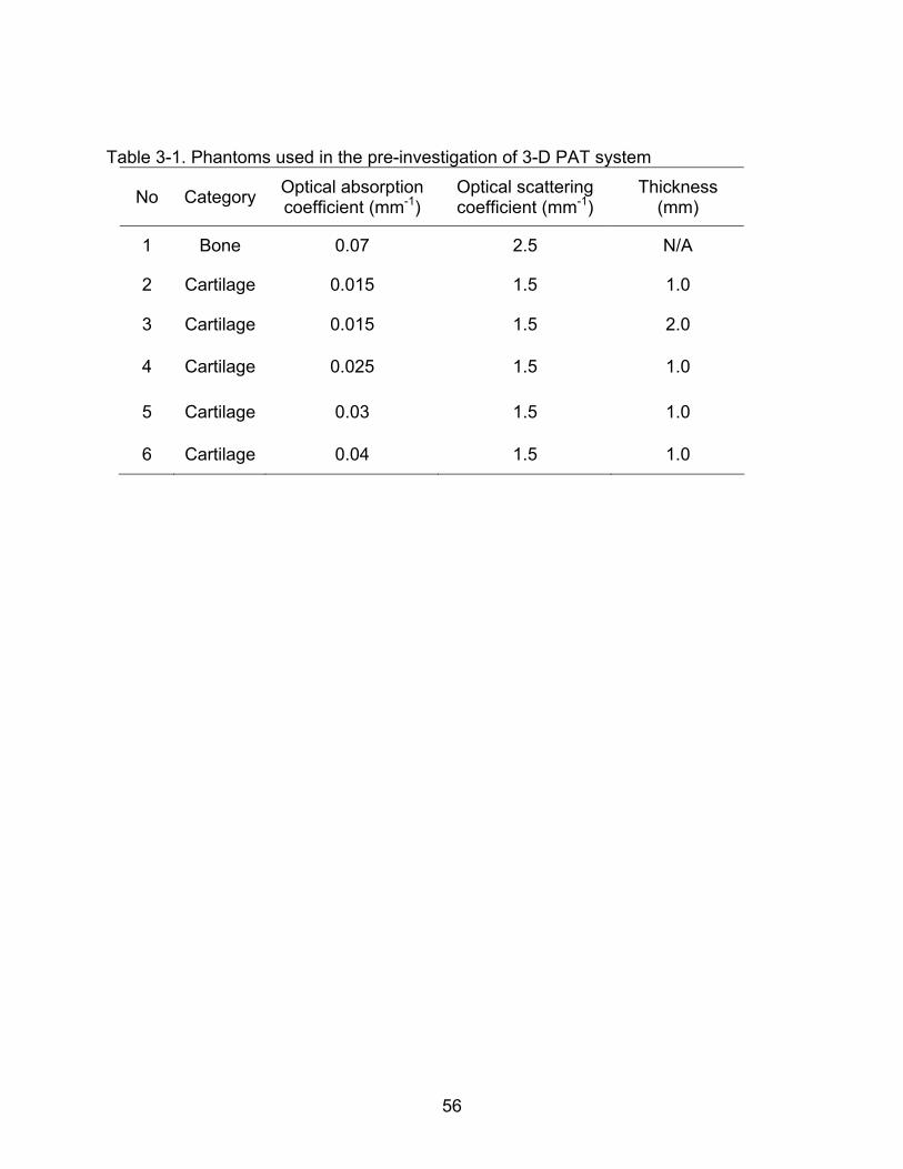
56

Table 3-1. Phantoms used in the pre-investigation of 3-D PAT system

No Category Optical absorption coefficient (mm-1)

Optical scattering coefficient (mm-1)

Thickness (mm)

1 Bone 0.07 2.5 N/A

2 Cartilage 0.015 1.5 1.0

3 Cartilage 0.015 1.5 2.0

4 Cartilage 0.025 1.5 1.0

5 Cartilage 0.03 1.5 1.0

6 Cartilage 0.04 1.5 1.0

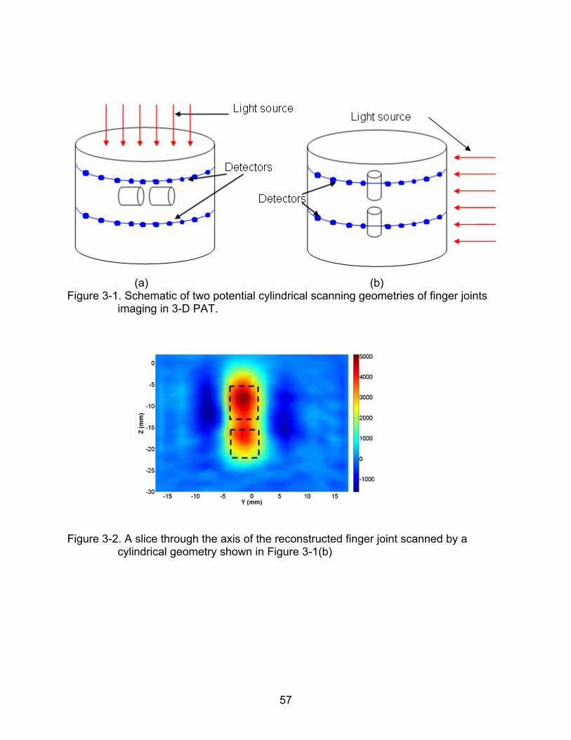
57

(a) (b) Figure 3-1. Schematic of two potential cylindrical scanning geometries of finger joints

imaging in 3-D PAT.

Figure 3-2. A slice through the axis of the reconstructed finger joint scanned by a

cylindrical geometry shown in Figure 3-1(b)

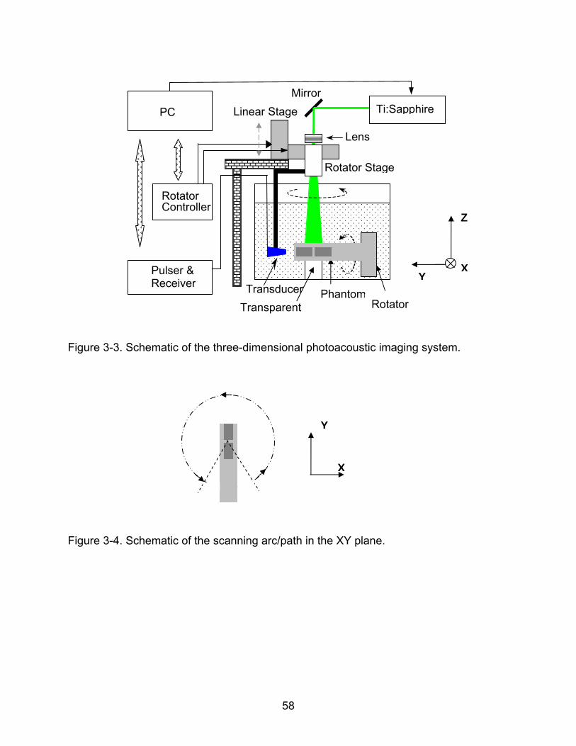
58

Figure 3-3. Schematic of the three-dimensional photoacoustic imaging system.

Figure 3-4. Schematic of the scanning arc/path in the XY plane.

PC

Rotator Stage

Mirror

Rotator Controller

Lens

Transducer

Pulser & Receiver

Phantom Rotator Transparent

Linear Stage

Z

YX

Ti:Sapphire

Y

X

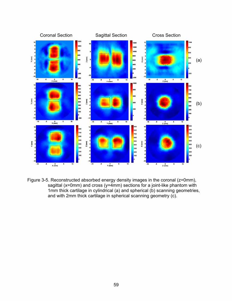
59

Coronal Section

Sagittal Section Cross Section

(a)

(b)

(c)

Figure 3-5. Reconstructed absorbed energy density images in the coronal (z=0mm),

sagittal (x=0mm) and cross (y=4mm) sections for a joint-like phantom with 1mm thick cartilage in cylindrical (a) and spherical (b) scanning geometries, and with 2mm thick cartilage in spherical scanning geometry (c).

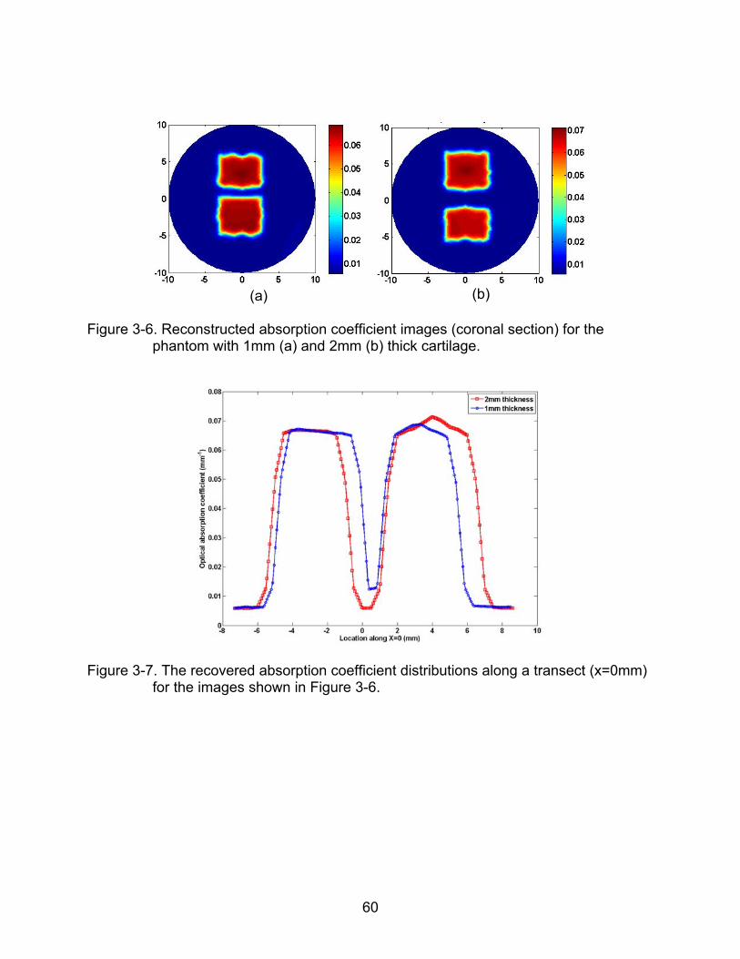
60

(a)

(b)

Figure 3-6. Reconstructed absorption coefficient images (coronal section) for the

phantom with 1mm (a) and 2mm (b) thick cartilage.

Figure 3-7. The recovered absorption coefficient distributions along a transect (x=0mm)

for the images shown in Figure 3-6.

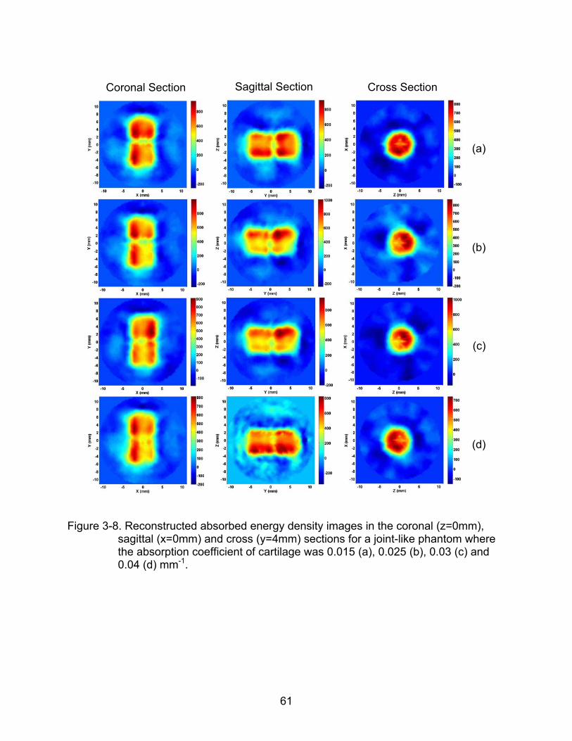
61

Coronal Section

Sagittal Section Cross Section

(a)

(b)

(c)

(d)

Figure 3-8. Reconstructed absorbed energy density images in the coronal (z=0mm),

sagittal (x=0mm) and cross (y=4mm) sections for a joint-like phantom where the absorption coefficient of cartilage was 0.015 (a), 0.025 (b), 0.03 (c) and 0.04 (d) mm-1.

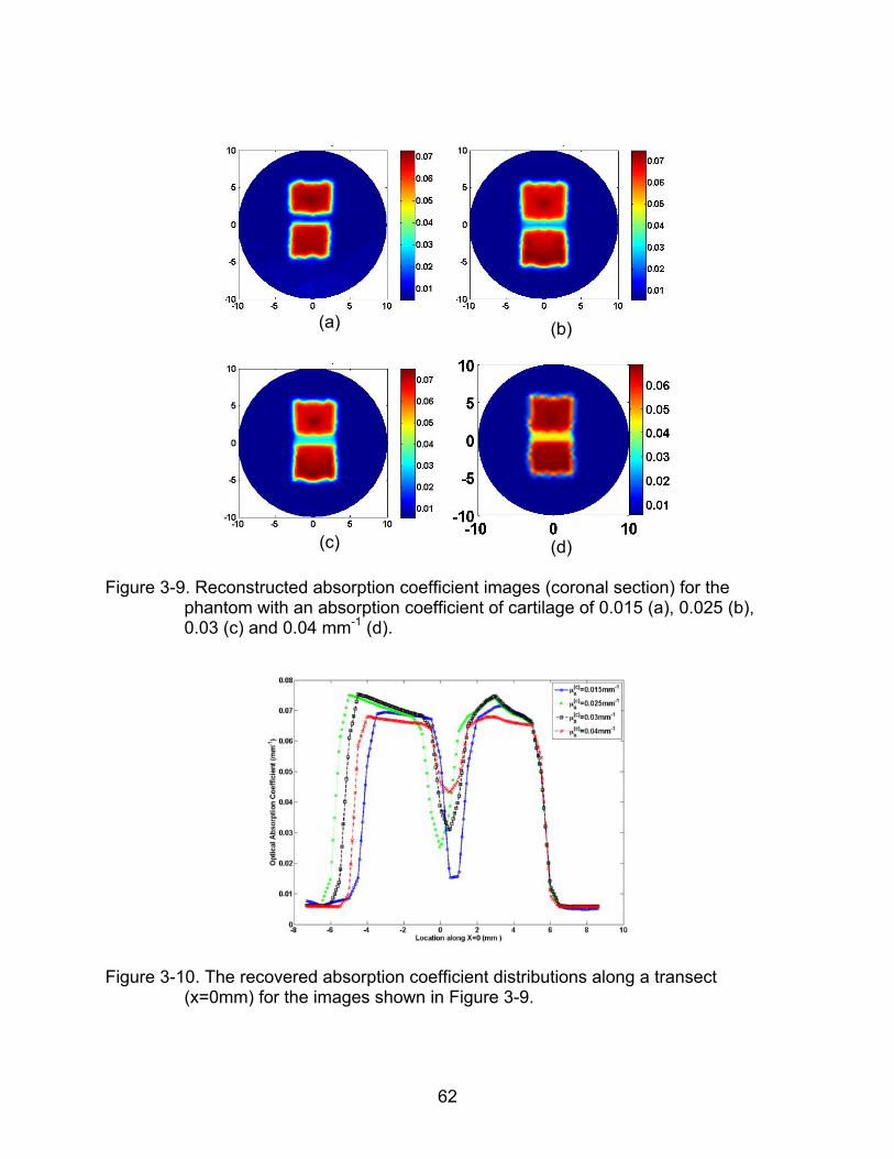
62

(a)

(b)

(c)

(d)

Figure 3-9. Reconstructed absorption coefficient images (coronal section) for the

phantom with an absorption coefficient of cartilage of 0.015 (a), 0.025 (b), 0.03 (c) and 0.04 mm-1 (d).

Figure 3-10. The recovered absorption coefficient distributions along a transect

(x=0mm) for the images shown in Figure 3-9.

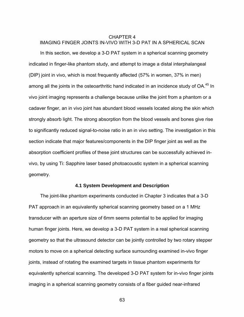
63

CHAPTER 4

IMAGING FINGER JOINTS IN-VIVO WITH 3-D PAT IN A SPHERICAL SCAN

In this section, we develop a 3-D PAT system in a spherical scanning geometry

indicated in finger-like phantom study, and attempt to image a distal interphalangeal

(DIP) joint in vivo, which is most frequently affected (57% in women, 37% in men)

among all the joints in the osteoarthritic hand indicated in an incidence study of OA.45 In

vivo joint imaging represents a challenge because unlike the joint from a phantom or a

cadaver finger, an in vivo joint has abundant blood vessels located along the skin which

strongly absorb light. The strong absorption from the blood vessels and bones give rise

to significantly reduced signal-to-noise ratio in an in vivo setting. The investigation in this

section indicate that major features/components in the DIP finger joint as well as the

absorption coefficient profiles of these joint structures can be successfully achieved in-

vivo, by using Ti: Sapphire laser based photoacoustic system in a spherical scanning

geometry.

4.1 System Development and Description

The joint-like phantom experiments conducted in Chapter 3 indicates that a 3-D

PAT approach in an equivalently spherical scanning geometry based on a 1 MHz

transducer with an aperture size of 6mm seems potential to be applied for imaging

human finger joints. Here, we develop a 3-D PAT system in a real spherical scanning

geometry so that the ultrasound detector can be jointly controlled by two rotary stepper

motors to move on a spherical detecting surface surrounding examined in-vivo finger

joints, instead of rotating the examined targets in tissue phantom experiments for

equivalently spherical scanning. The developed 3-D PAT system for in-vivo finger joints

imaging in a spherical scanning geometry consists of a fiber guided near-infrared

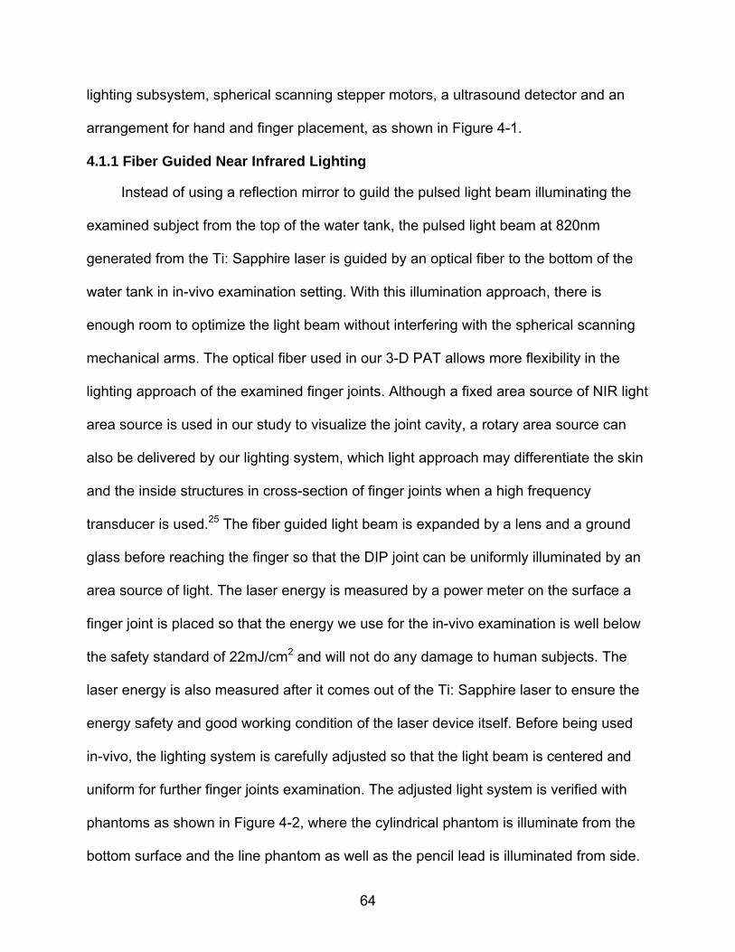
64

lighting subsystem, spherical scanning stepper motors, a ultrasound detector and an

arrangement for hand and finger placement, as shown in Figure 4-1.

4.1.1 Fiber Guided Near Infrared Lighting

Instead of using a reflection mirror to guild the pulsed light beam illuminating the

examined subject from the top of the water tank, the pulsed light beam at 820nm

generated from the Ti: Sapphire laser is guided by an optical fiber to the bottom of the

water tank in in-vivo examination setting. With this illumination approach, there is

enough room to optimize the light beam without interfering with the spherical scanning

mechanical arms. The optical fiber used in our 3-D PAT allows more flexibility in the

lighting approach of the examined finger joints. Although a fixed area source of NIR light

area source is used in our study to visualize the joint cavity, a rotary area source can

also be delivered by our lighting system, which light approach may differentiate the skin

and the inside structures in cross-section of finger joints when a high frequency

transducer is used.25 The fiber guided light beam is expanded by a lens and a ground

glass before reaching the finger so that the DIP joint can be uniformly illuminated by an

area source of light. The laser energy is measured by a power meter on the surface a

finger joint is placed so that the energy we use for the in-vivo examination is well below

the safety standard of 22mJ/cm2 and will not do any damage to human subjects. The

laser energy is also measured after it comes out of the Ti: Sapphire laser to ensure the

energy safety and good working condition of the laser device itself. Before being used

in-vivo, the lighting system is carefully adjusted so that the light beam is centered and

uniform for further finger joints examination. The adjusted light system is verified with

phantoms as shown in Figure 4-2, where the cylindrical phantom is illuminate from the

bottom surface and the line phantom as well as the pencil lead is illuminated from side.

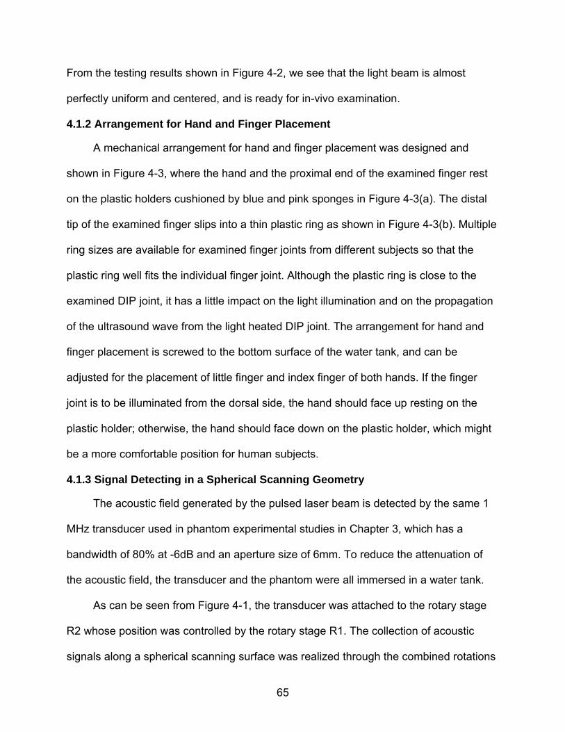
65

From the testing results shown in Figure 4-2, we see that the light beam is almost

perfectly uniform and centered, and is ready for in-vivo examination.

4.1.2 Arrangement for Hand and Finger Placement

A mechanical arrangement for hand and finger placement was designed and

shown in Figure 4-3, where the hand and the proximal end of the examined finger rest

on the plastic holders cushioned by blue and pink sponges in Figure 4-3(a). The distal

tip of the examined finger slips into a thin plastic ring as shown in Figure 4-3(b). Multiple

ring sizes are available for examined finger joints from different subjects so that the

plastic ring well fits the individual finger joint. Although the plastic ring is close to the

examined DIP joint, it has a little impact on the light illumination and on the propagation

of the ultrasound wave from the light heated DIP joint. The arrangement for hand and

finger placement is screwed to the bottom surface of the water tank, and can be

adjusted for the placement of little finger and index finger of both hands. If the finger

joint is to be illuminated from the dorsal side, the hand should face up resting on the

plastic holder; otherwise, the hand should face down on the plastic holder, which might

be a more comfortable position for human subjects.

4.1.3 Signal Detecting in a Spherical Scanning Geometry

The acoustic field generated by the pulsed laser beam is detected by the same 1

MHz transducer used in phantom experimental studies in Chapter 3, which has a

bandwidth of 80% at -6dB and an aperture size of 6mm. To reduce the attenuation of

the acoustic field, the transducer and the phantom were all immersed in a water tank.

As can be seen from Figure 4-1, the transducer was attached to the rotary stage

R2 whose position was controlled by the rotary stage R1. The collection of acoustic

signals along a spherical scanning surface was realized through the combined rotations

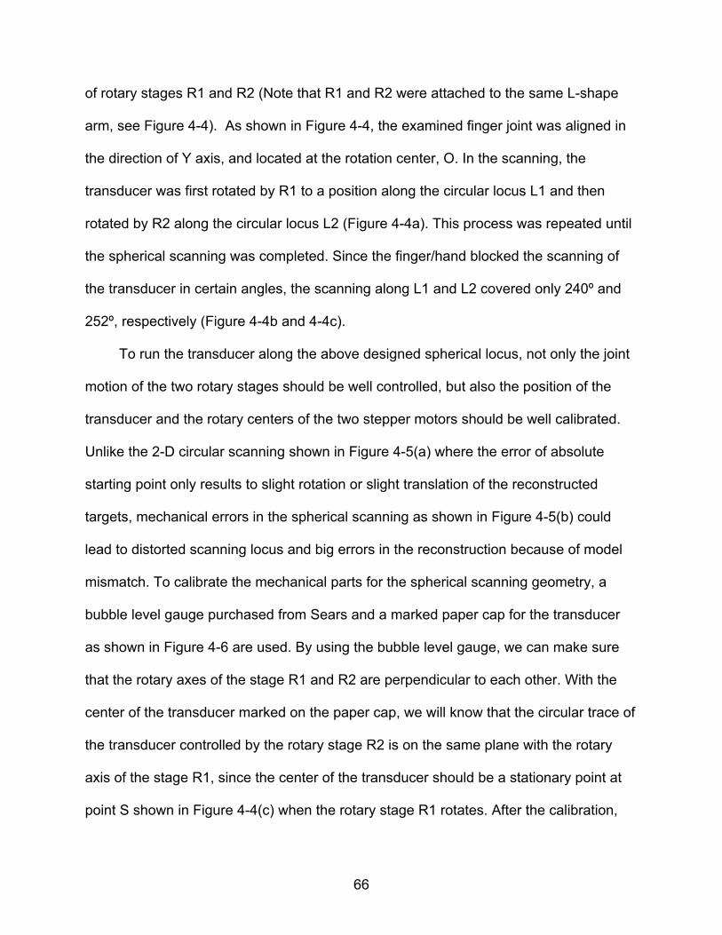
66

of rotary stages R1 and R2 (Note that R1 and R2 were attached to the same L-shape

arm, see Figure 4-4). As shown in Figure 4-4, the examined finger joint was aligned in

the direction of Y axis, and located at the rotation center, O. In the scanning, the

transducer was first rotated by R1 to a position along the circular locus L1 and then

rotated by R2 along the circular locus L2 (Figure 4-4a). This process was repeated until

the spherical scanning was completed. Since the finger/hand blocked the scanning of

the transducer in certain angles, the scanning along L1 and L2 covered only 240º and

252º, respectively (Figure 4-4b and 4-4c).

To run the transducer along the above designed spherical locus, not only the joint

motion of the two rotary stages should be well controlled, but also the position of the

transducer and the rotary centers of the two stepper motors should be well calibrated.

Unlike the 2-D circular scanning shown in Figure 4-5(a) where the error of absolute

starting point only results to slight rotation or slight translation of the reconstructed

targets, mechanical errors in the spherical scanning as shown in Figure 4-5(b) could

lead to distorted scanning locus and big errors in the reconstruction because of model

mismatch. To calibrate the mechanical parts for the spherical scanning geometry, a

bubble level gauge purchased from Sears and a marked paper cap for the transducer

as shown in Figure 4-6 are used. By using the bubble level gauge, we can make sure

that the rotary axes of the stage R1 and R2 are perpendicular to each other. With the

center of the transducer marked on the paper cap, we will know that the circular trace of

the transducer controlled by the rotary stage R2 is on the same plane with the rotary

axis of the stage R1, since the center of the transducer should be a stationary point at

point S shown in Figure 4-4(c) when the rotary stage R1 rotates. After the calibration,

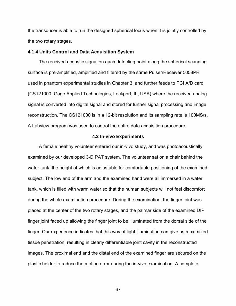
67

the transducer is able to run the designed spherical locus when it is jointly controlled by

the two rotary stages.

4.1.4 Units Control and Data Acquisition System

The received acoustic signal on each detecting point along the spherical scanning

surface is pre-amplified, amplified and filtered by the same Pulser/Receiver 5058PR

used in phantom experimental studies in Chapter 3, and further feeds to PCI A/D card

(CS121000, Gage Applied Technologies, Lockport, IL, USA) where the received analog

signal is converted into digital signal and stored for further signal processing and image

reconstruction. The CS121000 is in a 12-bit resolution and its sampling rate is 100MS/s.

A Labview program was used to control the entire data acquisition procedure.

4.2 In-vivo Experiments

A female healthy volunteer entered our in-vivo study, and was photoacoustically

examined by our developed 3-D PAT system. The volunteer sat on a chair behind the

water tank, the height of which is adjustable for comfortable positioning of the examined

subject. The low end of the arm and the examined hand were all immersed in a water

tank, which is filled with warm water so that the human subjects will not feel discomfort

during the whole examination procedure. During the examination, the finger joint was

placed at the center of the two rotary stages, and the palmar side of the examined DIP

finger joint faced up allowing the finger joint to be illuminated from the dorsal side of the

finger. Our experience indicates that this way of light illumination can give us maximized

tissue penetration, resulting in clearly differentiable joint cavity in the reconstructed

images. The proximal end and the distal end of the examined finger are secured on the

plastic holder to reduce the motion error during the in-vivo examination. A complete

68

scanning allowed the collection of signals at 387 positions along the spherical surface

which took about 40 minutes.

4.3 Methods

The collected photoacoustic signals in temporal domain were converted into

signals in frequency domain by Fourier Transforming for our finite element based 3-D

PAT reconstruction algorithm, which is based on finite element solution to the

photoacoustic wave equation in frequency domain subject to the radiation or absorbing

boundary conditions (BCs). The 3-D images of absorbed optical energy density were

reconstructed through our 3-D PAT reconstruction algorithm. The second step is to

recover the optical absorption coefficient distribution by using a forward fitting procedure

based on the photon diffusion model and the reconstructed absorbed optical energy

density images in the first step.29

The following photon diffusion equation as along with the Robin boundary

conditions can be used in the forward fitting procedure to recover the optical absorption

coefficient using the absorbed optical energy density reconstructed,

( ) ( ) ( ) ( ) ( )aD r r r r S r

(4.1)

ˆ( ) ( )D r n r

(4.2)

Where ( )r

is the photon density, ( ) ( ) / ( )ar r r

, ( )a r is the optical absorption

coefficient, ( )D r

is the diffusion coefficient, 1/(3( ))a sD and s is the reduced

scattering coefficients, is a boundary condition coefficient related to the internal

reflection at the boundary, and ( )S r

is the incident point or distributed source term.

To recover the optical absorption coefficient from the reconstructed absorbed

optical energy density from an initial distribution of ( )a r , the optical fluence ( )r

69

and the absorbed energy density ( )c are iteratively calculated through the photon

diffusion equation and ( ) ( )ca r

, respectively. If the error between and ( )c is

not small, then ( )a r is updated by ( ) ( ) / ( )a r r r

and the above procedure is

repeated until a small error between and ( )c is reached, resulting in a stable

quantitative distribution of ( )a r .

4.4 Results and Discussion

In this section, we present the in vivo 3-D reconstruction results and make

observations based on these results.

A coronal section of the reconstructed 3-D image (absorbed energy density) is

shown in Figure 4-7a, while a similar section of the DIP joint from a typical human finger

by MRI is given in Figure 4-7b for comparison. As can be observed from Figure 4-7a,

the cartilage/joint space is well differentiated from the adjacent distal phalanx (DP) and

intermediate phalanx (IP). The recovered absorption coefficient image and the

absorption coefficient profile along a transect X=-2mm corresponding to the coronal

slice shown in Figure 4-7a are displayed in Figure 4-8a and 4-8b, respectively. We see

that the absorption coefficient values of the phalanxes and cartilage/joint space are

quantitatively consistent with that reported in the literature. By estimating the full width

at half maximum (FWHM) of the absorption coefficient profiles, the recovered thickness

of cartilage/joint space was found to be 1.6mm, which is in agreement with the actual

size.

Figure 4-9a presents a cross section of the reconstructed 3-D image (absorbed

energy density). Again, a similar cross section of the DIP joint from a typical human

finger by MRI is shown in Figure 4-9b for comparison. Comparing both Figure 4-9a and

70

4-9b, it appears that several joint tissue types are visible including phalanx (PX), lateral

artery (LA) and median artery (MA), and tendon (TE). The recovered absorption

coefficient image and the absorption coefficient profiles along two transects are

displayed in Figure 4-10a to 4-10c. The first transect (line 1 in Figure 4-10a) goes

through the phalanx and tendon, while the second one (line 2 in Figure 4-10a) crosses

the tendon and two arteries. The recovered absorption coefficients of the phalanx,

tendon, median and lateral arteries were found to be 0.07mm-1, 0.074mm-1, 0.064mm-1

and 0.058mm-1, respectively. Again, these values are generally consistent with that

reported in the literature. We note that blurs around the two blood vessels are

noticeable (Figure 4-10a), largely due to the relatively low-frequency (1MHz) transducer

used in this study. We believe the resolution can be enhanced with a wideband

transducer having higher frequency (e.g., 5-10MHz) which will make the millimeter-

submillimeter sized arteries accurately imaged.

To view the volumetric structures of the tissues around the joint, a series of cross

and coronal section images are displayed in Figure 4-11 and 4-12, respectively. As

shown in Figure 4-11a to 1-11f, the phalanx is clearly visible in all the cross section

images from the proximal end (Y=-2.5mm) to the distal end (Y=9mm). The tendon is

differentiated from the phalanx (Figure 4-11a, 4-11e and 4-11f). The lateral artery is

visible almost in all the cross section images except for that shown in Figure 4-11f at the

distal end of the finger. The median artery is seen in Figure 4-11e and Figure 4-11f, and

weakly visible in Figure 4-11d. Other joint structures including the phalanges (DP and IP)

and the cartilage (CL) are clearly imaged from the coronal section images close to the

dorsal side of the finger (Figure 4-12a and 4-12b). Close to the palmar side of the finger,

71

the tendon and two arteries begin to show up (Figure 4-12c), and the two arteries

eventually become clearly visible (Figure 4-12d). Negative values are also observed in

the reconstructed absorbed energy density images. It is likely due to the homogenous

acoustic approximation (constant acoustic speed) to the actual heterogeneous acoustic

media of the finger joints and limited signal-to-noise ratio because of the strong light

scattering of joint tissues.

In summary, we have presented a 3-D PAT technique that is able to image finger

joints in vivo. Although it seems impossible for PAT to provide image quality (in terms of

spatial resolution) comparable to MRI for joint or breast imaging, PAT is capable of

obtaining absorption coefficient or functional information. In addition, PAT is portable

and low in cost. While our current experimental setup is not optimized, it allows us to

demonstrate the possibility of 3-D in vivo joint imaging for the first time. The results

obtained indicate that major joint structures and their absorption coefficients can be

quantitatively reconstructed using our 3-D PAT approach.

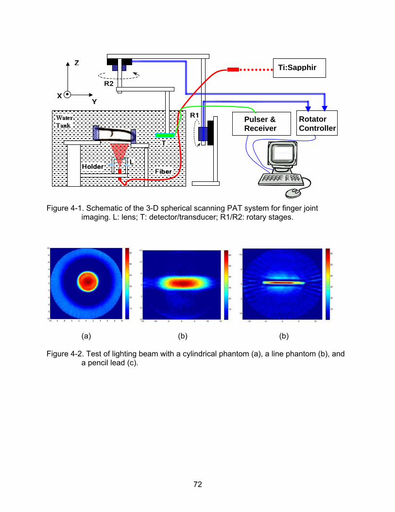
72

Figure 4-1. Schematic of the 3-D spherical scanning PAT system for finger joint imaging. L: lens; T: detector/transducer; R1/R2: rotary stages.

(a) (b) (b)

Figure 4-2. Test of lighting beam with a cylindrical phantom (a), a line phantom (b), and a pencil lead (c).

Z

YX

Pulser & Receiver

Rotator Controller

Ti:Sapphir

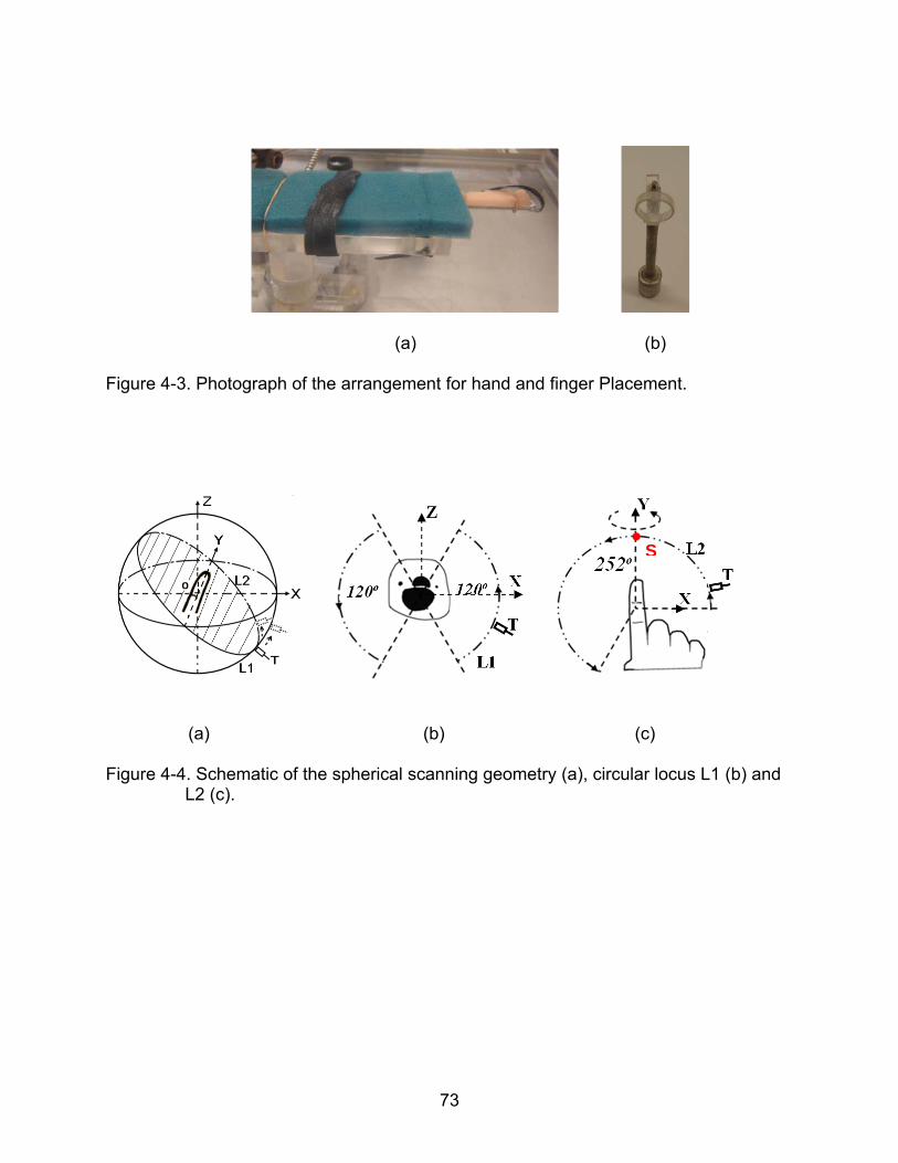
73

(a) (b)

Figure 4-3. Photograph of the arrangement for hand and finger Placement.

(a) (b) (c)

Figure 4-4. Schematic of the spherical scanning geometry (a), circular locus L1 (b) and

L2 (c).

S

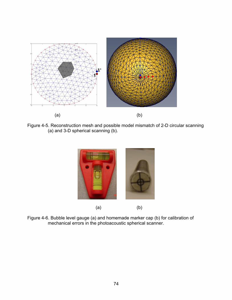
74

(a) (b)

Figure 4-5. Reconstruction mesh and possible model mismatch of 2-D circular scanning (a) and 3-D spherical scanning (b).

(a) (b)

Figure 4-6. Bubble level gauge (a) and homemade marker cap (b) for calibration of mechanical errors in the photoacoustic spherical scanner.

1’1

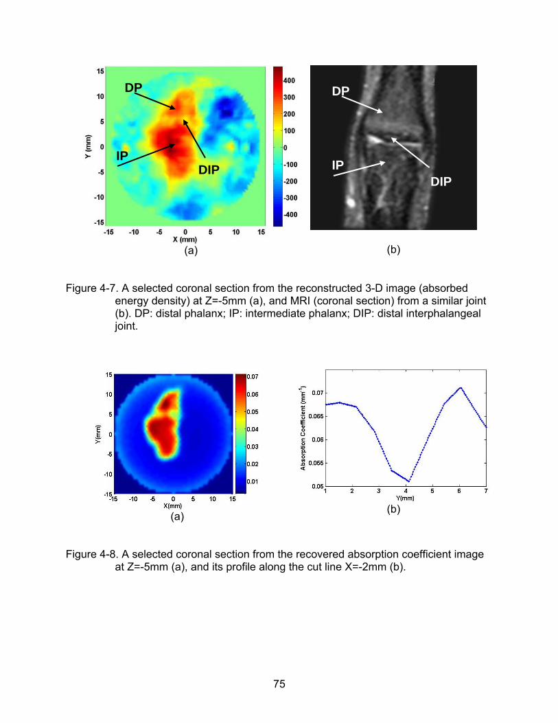
75

(a)

(b)

Figure 4-7. A selected coronal section from the reconstructed 3-D image (absorbed energy density) at Z=-5mm (a), and MRI (coronal section) from a similar joint (b). DP: distal phalanx; IP: intermediate phalanx; DIP: distal interphalangeal joint.

(a)

(b)

Figure 4-8. A selected coronal section from the recovered absorption coefficient image at Z=-5mm (a), and its profile along the cut line X=-2mm (b).

DP

IP DIP

DP

IP DIP

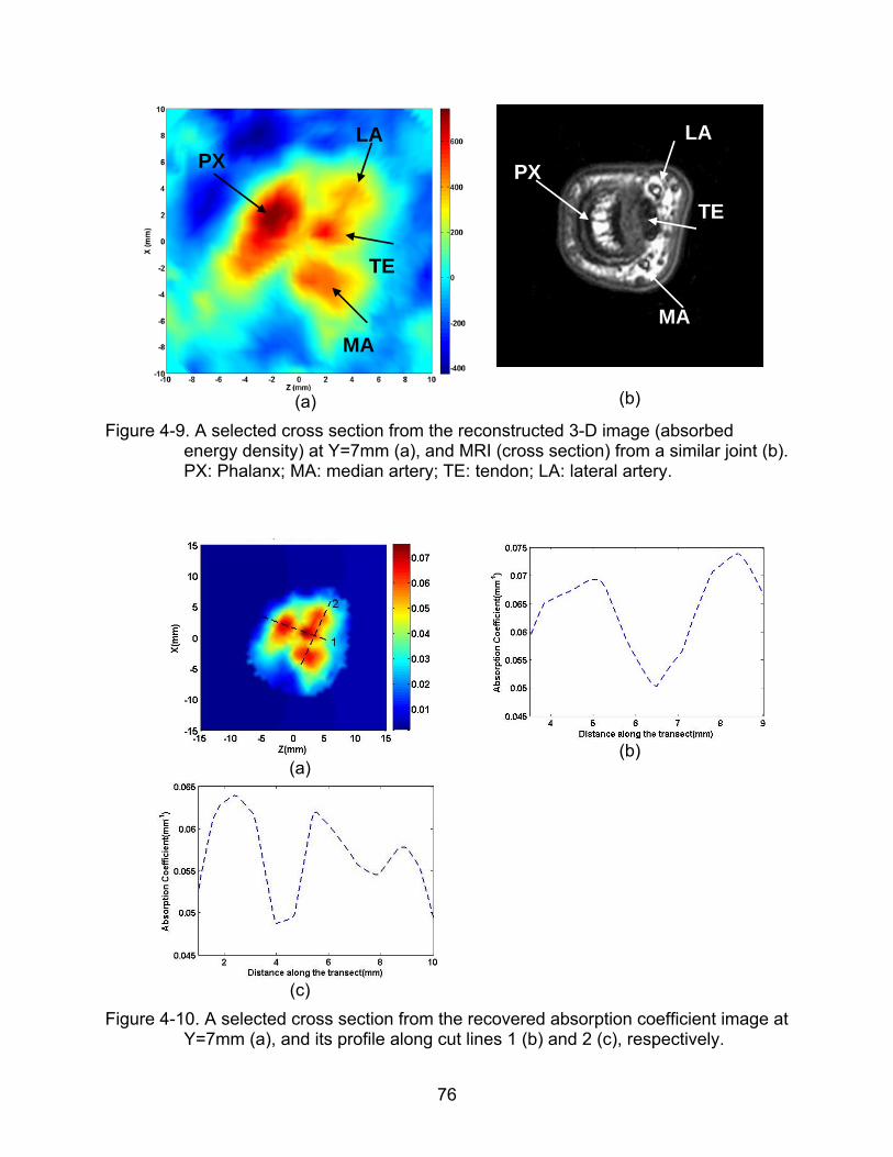
76

(a)

(b)

Figure 4-9. A selected cross section from the reconstructed 3-D image (absorbed energy density) at Y=7mm (a), and MRI (cross section) from a similar joint (b). PX: Phalanx; MA: median artery; TE: tendon; LA: lateral artery.

(a)

(b)

(c)

Figure 4-10. A selected cross section from the recovered absorption coefficient image at Y=7mm (a), and its profile along cut lines 1 (b) and 2 (c), respectively.

PX LA

MA

TE

PX

LA

MA

TE

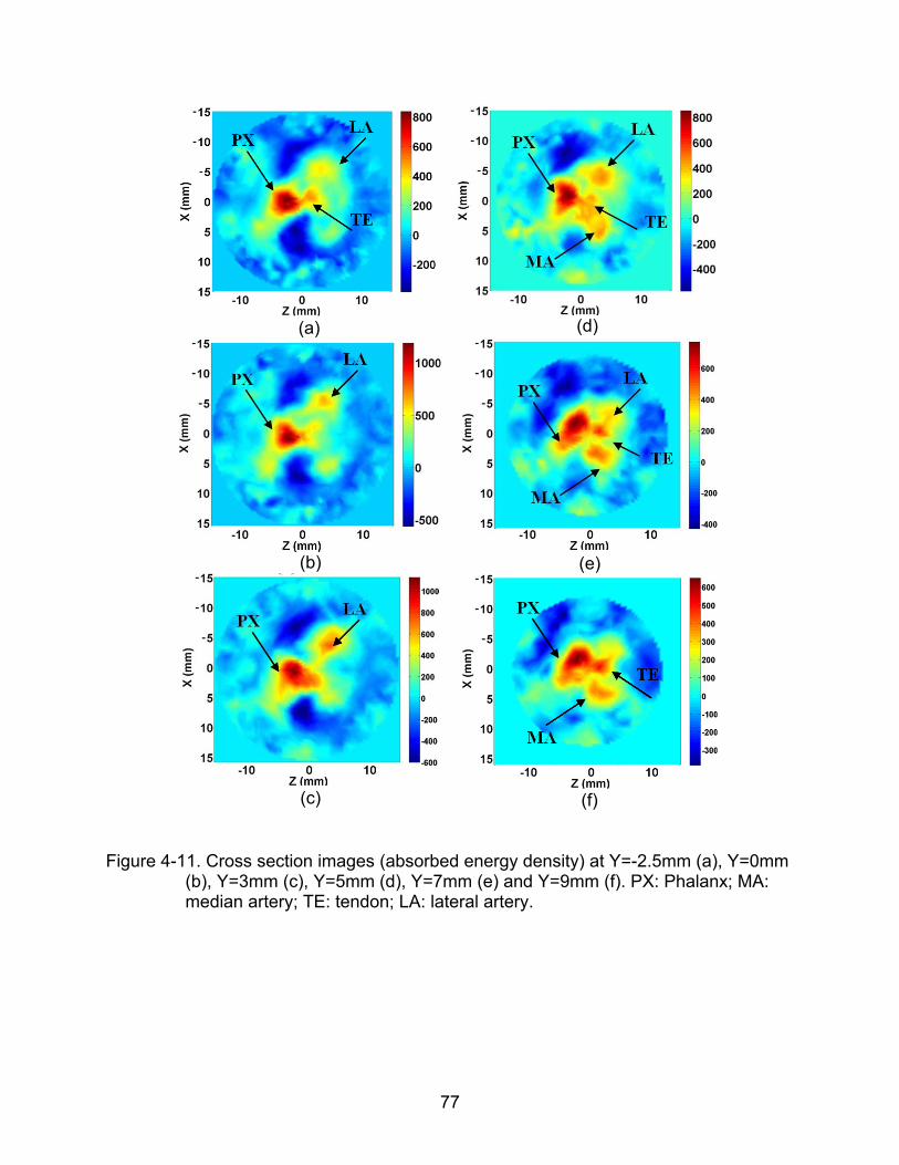
77

(a)

(d)

(b)

(e)

(c)

(f)

Figure 4-11. Cross section images (absorbed energy density) at Y=-2.5mm (a), Y=0mm (b), Y=3mm (c), Y=5mm (d), Y=7mm (e) and Y=9mm (f). PX: Phalanx; MA: median artery; TE: tendon; LA: lateral artery.

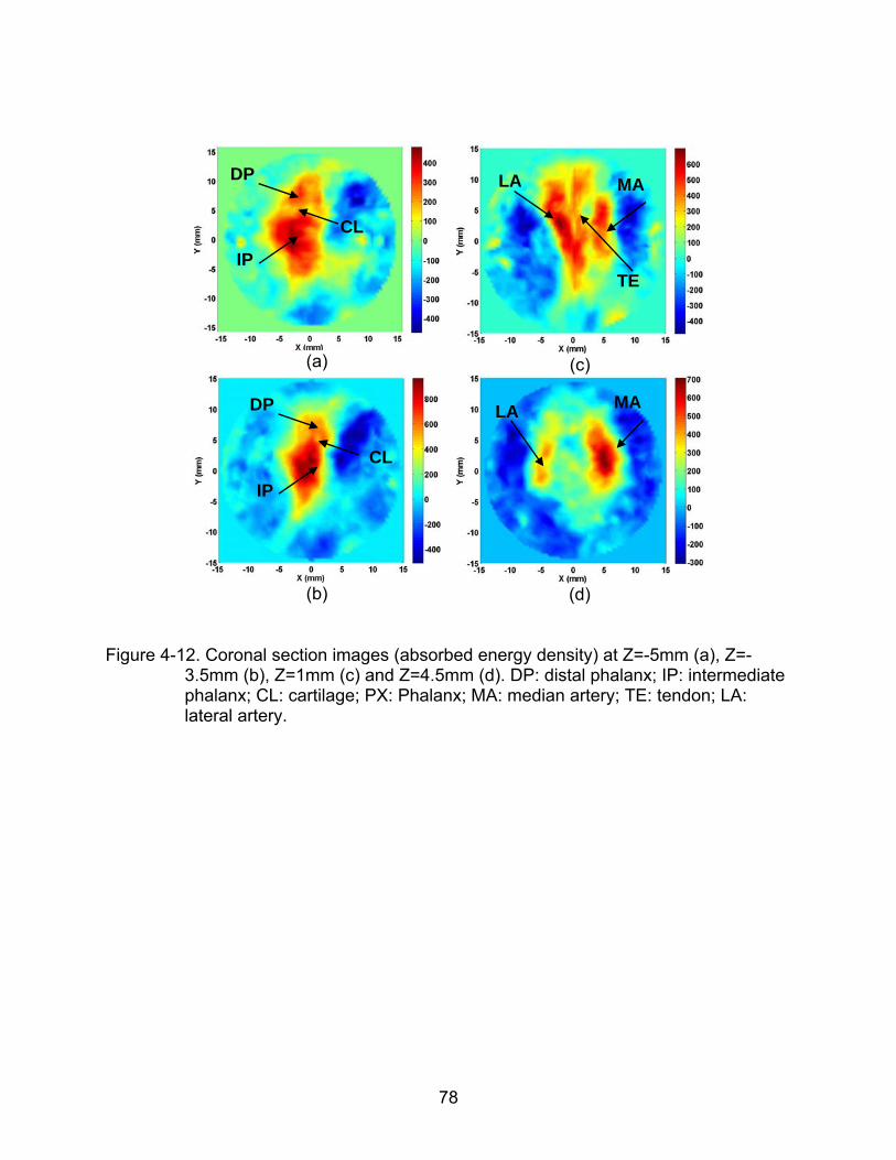
78

(a)

(c)

(b)

(d)

Figure 4-12. Coronal section images (absorbed energy density) at Z=-5mm (a), Z=-3.5mm (b), Z=1mm (c) and Z=4.5mm (d). DP: distal phalanx; IP: intermediate phalanx; CL: cartilage; PX: Phalanx; MA: median artery; TE: tendon; LA: lateral artery.

LA MA

DP

IP

CL

DP

IP

CL

LA MA

TE

79

CHAPTER 5 CLINCAL EXAMINATION OF OA PATIENTS WITH 3-D PAT

Osteoarthritis (OA) is the most common degenerative joint disease, which affects

tens of millions of Americans. Although knee and hip OA bear most responsibility for the

burden of OA, hand OA may be a marker of a systemic predisposition toward OA;

Incidence study of OA further revealed that the second DIP joint is most frequently

affected (57% in women, 37% in men) among all the joints in the hand.45

Thus far, clinical examination remains the principal approach of OA diagnosis,

relying on symptoms and signs OA patients suffered as well as experience of arthritis

physicians. Imaging techniques, including standard x-ray radiography, computed

tomography (CT), ultrasonography and magnetic resonance imaging (MRI), are used

only as supplemental methods in OA diagnosis, especially in hand OA, either because

they are insensitive to the abnormal changes in the OA joint cavity or because they are

too costly to be used as a routine examination method. As such, sensitive and

affordable imaging methods are urgently needed for the detection of OA, especially in

early stage. Moreover, the progress of effective imaging methods in OA diagnosis may

at the same time accelerate the advancement of medical therapies for OA, which are

currently effective to relief OA symptoms or prevent the worsening of OA in certain

degree and yet of limited effectiveness in modifying OA. Up to now, no approved

disease-modifying OA drugs (DMOADs) are available, development of which may

benefit greatly from the progress of imaging methods in OA diagnosis, where sensitive

imaging techniques can serve as surrogate markers for clinically meaningful outcomes

to economically and efficiently validate the candidate DMOADs.43

80

New imaging techniques based on near-infrared (NIR) light, including pure-optical

imaging techniques and photoacoustic tomography (PAT), has been recently studied to

image finger joints and to effectively detect joint diseases.4-7,25, 55-57 While optical

imaging techniques are able to detect the highly sensitive optical absorption / scattering

abnormalities associated with soft tissues (cartilage, synovial fluid, etc) in OA and RA

joints, its spatial resolution is relatively low (about 3~5mm). Compared to all-optical

imaging techniques, PAT is able to visualize the same optical absorption contrast with

significantly improved spatial resolution (0.5mm or better, adjustable with ultrasound

frequency) for deep-tissue imaging.

In this section, we take the advantage of the high spatial resolution provided by

PAT technique in imaging the optical absorption property, continue previous study in

finger joints imaging using 3-D PAT in a spherical scanning geometry, and present a

pilot clinical study of detecting OA using 3-D PAT on both osteoarthritis patients and

healthy controls.

5.1 Enhancement in 3-D PAT Approach

In the in-vivo finger joints imaging conducted in Chapter 5, a single 1MHz

transducer is used to receive the generated ultrasound signals, and then is feed into a

single channel signal processing unit (preamplifier, amplifier, filter, and A/D conversion).

The whole procedure of examination lasts about 40 minutes with single channel

detecting system, which is too long for OA patients. To speed up the examination

process, an ultrasound detection array together with multiple channel signal processing

unit is designed, calibrated and tested with tissue-like phantom experiments. With

multiple channel detection system, the examination of a finger joint can be completed in

5 minutes, allowing the collection of photoacoustic signals at 360 positions surrounding

81

the examined DIP joint. DIP finger joints from OA patients and healthy volunteers are

further imaged with our enhanced 3-D PAT system in a spherical scanning configuration,

which are comprised of a pulsed NIR light source as same as the one in in-vivo finger

joint imaging conducted in Chapter 4, a spherical scanning subsystem, and an

ultrasound detection array and associated data acquisition system as shown in Figure

5-1.

5.1.1 Ultrasound Detection Array

The ultrasound detection array (photograph shown in Figure 5-1 and the design

shown in Figure 5-2) is composed of eight 1 MHz transducers (Valpey Fisher,

Hopkinton, MA) arranged uniformly along a 210o circular arc. The transducer has a

bandwidth of 80% at -6dB and an aperture size of 6mm. The position and performance

of each transducer in the ultrasound array has to be calibrated carefully before

experimental study. Ideally, the rotation of ultrasound detecting array in certain degrees

in the plane where all the transducer elements are arranged should result in the overlap

of the positions and received acoustic signals between different transducer elements.

For example, positions and received signals from transducer T1, T2 until T7 after being

counterclockwise rotated in 30o (together with rotary stage R2) should coincide with

those from transducer T2, T3 until T8 shown in Figure 5-2 before the ultrasound

detecting array was rotated.

In calibrating the system errors in mechanical parts, the center of the ultrasound

detector array must coincide with the rotation axis of the rotary stage R2, and the plane

where all the transducer elements are securely arranged should be perpendicular with

the rotation axis of the rotary stage R2, so that the rotary motion of R2 will not cause

evident position error between transducer elements shown in Figure 5-3. After the

82

calibration between the center of the ultrasound detecting array and the rotary center of

the stage R2, the position of each transducer element has to be precisely aligned and

secured in the ultrasound detecting array so that each transducer element is in the

same distance from the center of the ultrasound detecting array. The position calibration

of each transducer element is conducted by measuring the pulse-echo response of the

each transducer element from a fixed reflection surface, as shown in Figure 5-4(a)

where pulse-echo responses of fours selected transducer elements are measured in

50MHz sampling rate. From the responses shown in Figure 5-4 (a), location variations

between the four transducer elements are observed and require fine alignment so that

the four pulse-echo responses are of the same flight of time (in the same dashed

vertical line as shown in Figure 5-4(a)). The alignment errors of the transducer elements

can be limited within 0.2mm (about 7 sampling points’ variation) by observing the above

pulse-echo responses. The sensitivities and impulse responses of the transducer

elements may also exhibit some differences, which result in the amplitude fluctuation

and slight spectrum shift shown in Figure 5-4(b). We measured the received acoustic

signals of each element on the same location with a well-controlled phantom experiment

and calculated the performance calibration coefficients of all the transducer elements,

which are used in the signal calibration of each experiment conducted with this system.

The same method as employed in Chapter 4 is used to calibrate the altitude of the

plane where all the transducer elements are securely arranged. With the marked cap

shown in Figure 4-6(b), the transducer elements can be finely elevated on the same

plane with the rotary axis of the stage R1 since the center of the transducer element at

point F shown in Figure 5-2 should be a stationary point when the stage R1 rotates.

83

5.1.2 Multiple Channel Data Acquisition

The detected acoustic signals were feed into preamplifiers and converted to digital

signals by an A/D board (PREAMP2-D and PCIAD1650, US Ultratek, Concord, CA), as

shown in the block diagram of the multiple-channel 3-D PAT system (Figure 5-5). Two

preamplifier sets (PREAMP2-D) are used in our 3-D PAT system, each including four

pre-amplifying channels. The preamplifier PREAMP2-D has a bandwidth from 20 KHz to

30MHz at -3dB, with a gain range from 10 to 60dB. The signal to Noise Ratio of the

preamplifier is 67dB. The PCI card PCIAD1650 consists of 16 pulse/receiver channels,

each of which is integrated with an amplifier (0 dB to 80 dB in 0.01dB increments) and a

signal filter (low pass from 5.9MHz to 48MHz, and high pass from 16 KHz to 4.8MHz).

The sampling rate of the PCIAD1650 is tunable from 390.625 KHz up to 50MHz (8

scales). The central values of the pulse/receiver channels have some variation as

shown in Figure 5-6(a), and require relative calibration between the detecting channels.

The multiple channels A/D board and the entire examination procedure are controlled

by a Labview interface shown in Figure 5-6(b), which include the initiation of step motor

controllers, procession of the spherical scanner(ultrasound detecting array),

communication between the interface with the PCIAD1650, and signal display/storage.

5.1.3 Quantitative 3-D PAT with 3-D Photon Diffusion Model

A forward fitting procedure based on the 3-D photon diffusion model and the

reconstructed 3-D absorbed optical energy density images in 3-D PAT is used to

recover the three-dimensional images of optical absorption coefficient distribution, which

is important for further quantitative analysis of the full joint. This forward fitting method

requires no segmentation and is relatively easy to implement. 29To recover the optical

absorption coefficient from the reconstructed absorbed optical energy density ( )r

from

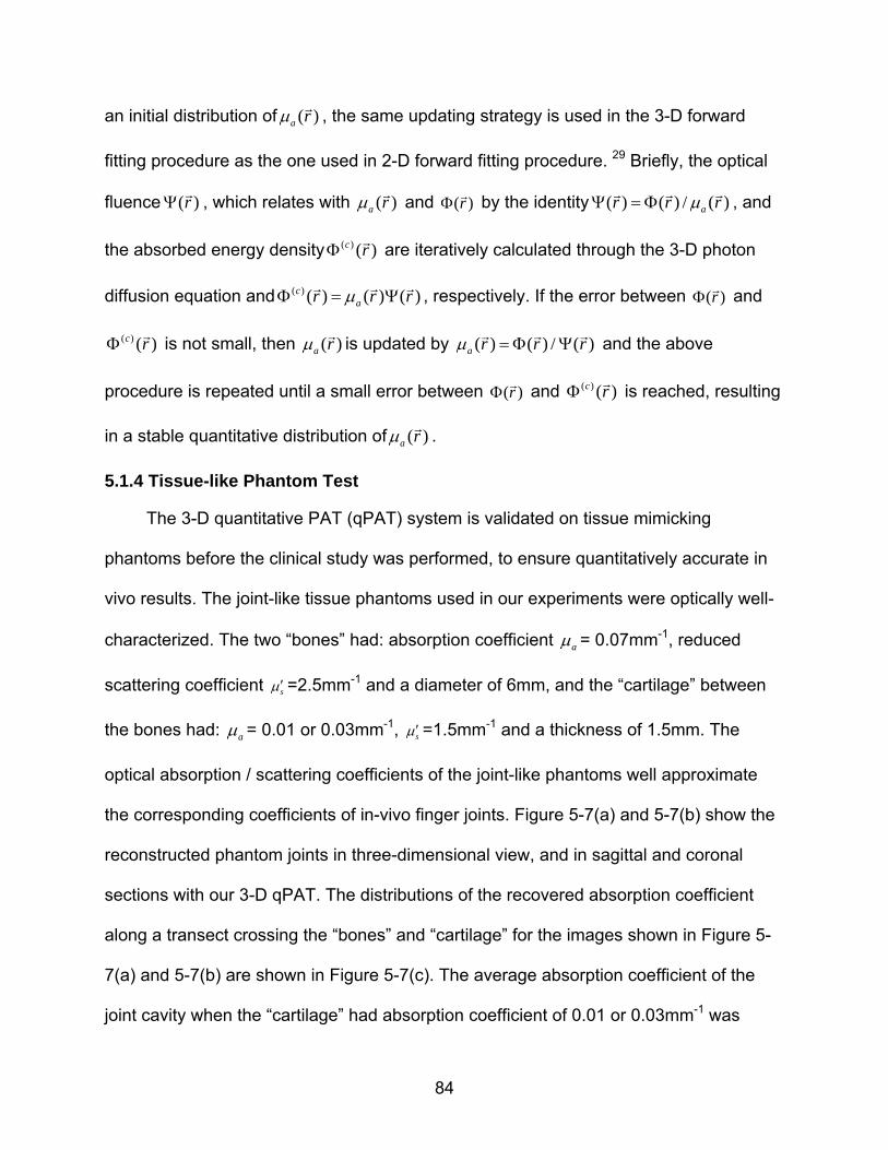
84

an initial distribution of ( )a r , the same updating strategy is used in the 3-D forward

fitting procedure as the one used in 2-D forward fitting procedure. 29 Briefly, the optical

fluence ( )r

, which relates with ( )a r and ( )r

by the identity ( ) ( ) / ( )ar r r

, and

the absorbed energy density ( ) ( )c r

are iteratively calculated through the 3-D photon

diffusion equation and ( ) ( ) ( ) ( )car r r

, respectively. If the error between ( )r

and

( ) ( )c r

is not small, then ( )a r is updated by ( ) ( ) / ( )a r r r

and the above

procedure is repeated until a small error between ( )r

and ( ) ( )c r

is reached, resulting

in a stable quantitative distribution of ( )a r .

5.1.4 Tissue-like Phantom Test

The 3-D quantitative PAT (qPAT) system is validated on tissue mimicking

phantoms before the clinical study was performed, to ensure quantitatively accurate in

vivo results. The joint-like tissue phantoms used in our experiments were optically well-

characterized. The two “bones” had: absorption coefficient a = 0.07mm-1, reduced

scattering coefficient s=2.5mm-1 and a diameter of 6mm, and the “cartilage” between

the bones had: a = 0.01 or 0.03mm-1, s=1.5mm-1 and a thickness of 1.5mm. The

optical absorption / scattering coefficients of the joint-like phantoms well approximate

the corresponding coefficients of in-vivo finger joints. Figure 5-7(a) and 5-7(b) show the

reconstructed phantom joints in three-dimensional view, and in sagittal and coronal

sections with our 3-D qPAT. The distributions of the recovered absorption coefficient

along a transect crossing the “bones” and “cartilage” for the images shown in Figure 5-

7(a) and 5-7(b) are shown in Figure 5-7(c). The average absorption coefficient of the

joint cavity when the “cartilage” had absorption coefficient of 0.01 or 0.03mm-1 was

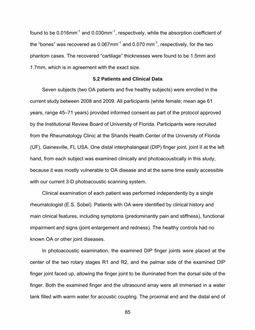
85

found to be 0.016mm-1 and 0.030mm-1, respectively, while the absorption coefficient of

the “bones” was recovered as 0.067mm-1 and 0.070 mm-1, respectively, for the two

phantom cases. The recovered “cartilage” thicknesses were found to be 1.5mm and

1.7mm, which is in agreement with the exact size.

5.2 Patients and Clinical Data

Seven subjects (two OA patients and five healthy subjects) were enrolled in the

current study between 2008 and 2009. All participants (white female; mean age 61

years, range 45–71 years) provided informed consent as part of the protocol approved

by the Institutional Review Board of University of Florida. Participants were recruited

from the Rheumatology Clinic at the Shands Health Center of the University of Florida

(UF), Gainesville, FL USA. One distal interphalangeal (DIP) finger joint, joint II at the left

hand, from each subject was examined clinically and photoacoustically in this study,

because it was mostly vulnerable to OA disease and at the same time easily accessible

with our current 3-D photoacoustic scanning system.

Clinical examination of each patient was performed independently by a single

rheumatologist (E.S. Sobel). Patients with OA were identified by clinical history and

main clinical features, including symptoms (predominantly pain and stiffness), functional

impairment and signs (joint enlargement and redness). The healthy controls had no

known OA or other joint diseases.

In photoacoustic examination, the examined DIP finger joints were placed at the

center of the two rotary stages R1 and R2, and the palmar side of the examined DIP

finger joint faced up, allowing the finger joint to be illuminated from the dorsal side of the

finger. Both the examined finger and the ultrasound array were all immersed in a water

tank filled with warm water for acoustic coupling. The proximal end and the distal end of

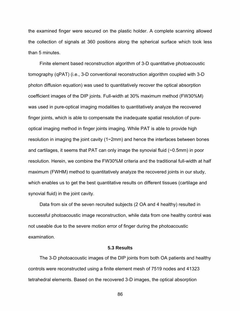
86

the examined finger were secured on the plastic holder. A complete scanning allowed

the collection of signals at 360 positions along the spherical surface which took less

than 5 minutes.

Finite element based reconstruction algorithm of 3-D quantitative photoacoustic

tomography (qPAT) (i.e., 3-D conventional reconstruction algorithm coupled with 3-D

photon diffusion equation) was used to quantitatively recover the optical absorption

coefficient images of the DIP joints. Full-width at 30% maximum method (FW30%M)

was used in pure-optical imaging modalities to quantitatively analyze the recovered

finger joints, which is able to compensate the inadequate spatial resolution of pure-

optical imaging method in finger joints imaging. While PAT is able to provide high

resolution in imaging the joint cavity (1~2mm) and hence the interfaces between bones

and cartilages, it seems that PAT can only image the synovial fluid (~0.5mm) in poor

resolution. Herein, we combine the FW30%M criteria and the traditional full-width at half

maximum (FWHM) method to quantitatively analyze the recovered joints in our study,

which enables us to get the best quantitative results on different tissues (cartilage and

synovial fluid) in the joint cavity.

Data from six of the seven recruited subjects (2 OA and 4 healthy) resulted in

successful photoacoustic image reconstruction, while data from one healthy control was

not useable due to the severe motion error of finger during the photoacoustic

examination.

5.3 Results

The 3-D photoacoustic images of the DIP joints from both OA patients and healthy

controls were reconstructed using a finite element mesh of 7519 nodes and 41323

tetrahedral elements. Based on the recovered 3-D images, the optical absorption

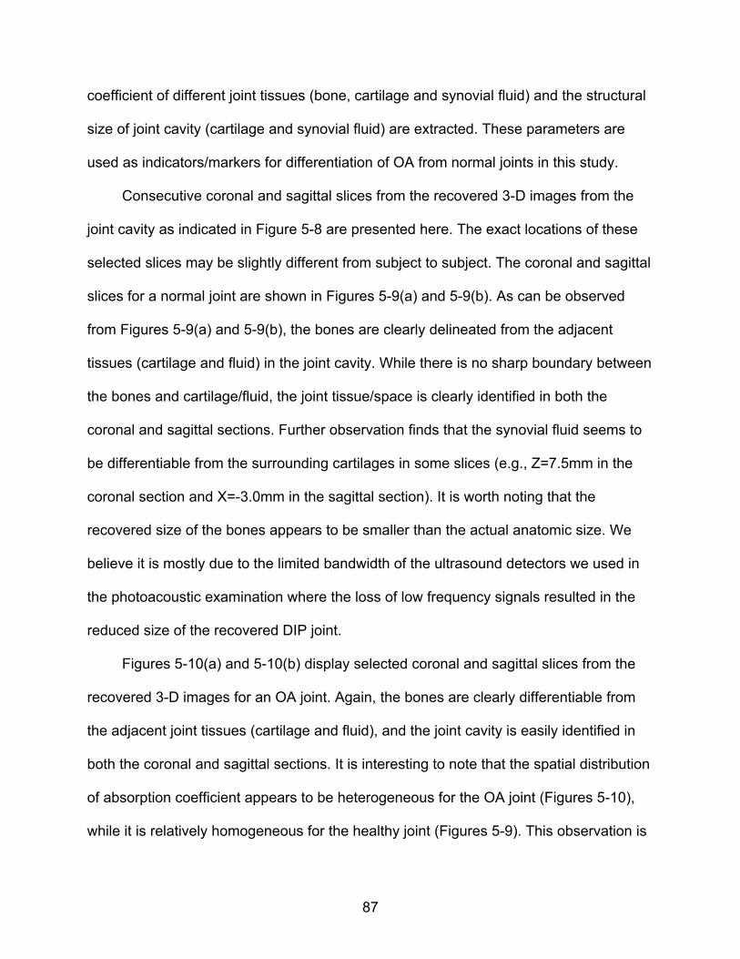
87

coefficient of different joint tissues (bone, cartilage and synovial fluid) and the structural

size of joint cavity (cartilage and synovial fluid) are extracted. These parameters are

used as indicators/markers for differentiation of OA from normal joints in this study.

Consecutive coronal and sagittal slices from the recovered 3-D images from the

joint cavity as indicated in Figure 5-8 are presented here. The exact locations of these

selected slices may be slightly different from subject to subject. The coronal and sagittal

slices for a normal joint are shown in Figures 5-9(a) and 5-9(b). As can be observed

from Figures 5-9(a) and 5-9(b), the bones are clearly delineated from the adjacent

tissues (cartilage and fluid) in the joint cavity. While there is no sharp boundary between

the bones and cartilage/fluid, the joint tissue/space is clearly identified in both the

coronal and sagittal sections. Further observation finds that the synovial fluid seems to

be differentiable from the surrounding cartilages in some slices (e.g., Z=7.5mm in the

coronal section and X=-3.0mm in the sagittal section). It is worth noting that the

recovered size of the bones appears to be smaller than the actual anatomic size. We

believe it is mostly due to the limited bandwidth of the ultrasound detectors we used in

the photoacoustic examination where the loss of low frequency signals resulted in the

reduced size of the recovered DIP joint.

Figures 5-10(a) and 5-10(b) display selected coronal and sagittal slices from the

recovered 3-D images for an OA joint. Again, the bones are clearly differentiable from

the adjacent joint tissues (cartilage and fluid), and the joint cavity is easily identified in

both the coronal and sagittal sections. It is interesting to note that the spatial distribution

of absorption coefficient appears to be heterogeneous for the OA joint (Figures 5-10),

while it is relatively homogeneous for the healthy joint (Figures 5-9). This observation is

88

consistent with the findings from the previous optical imaging study. Compared with the

healthy joint (Figures 5-9), the joint space narrowing seems apparent for the OA joint

(Figures 5-10).

The average absorption coefficient and structural size of joint tissues for all the

subjects are calculated and presented in Tables 5-1. We note from Table 1 that the

recovered absorption coefficient of the diseased synovial fluid ranges from 0.022 to

0.023mm-1, while it is below 0.017mm-1 (0.0089 to 0.017mm-1) for the normal fluid.

Difference between OA joints and healthy controls is also apparent, in terms of the

absorption coefficient of the synovial fluid in the joint cavity. The difference is more

striking when the ratio of the absorption coefficient of the synovial fluid to that of the

bone is considered (0.58~0.63 for OA joints verse 0.25~0.46 for normal joints). For the

diseased cartilage, the absorption coefficient (0.026~0.028mm-1) is generally larger than

that of normal joints (0.015~0.024mm-1). The ratio of the absorption coefficient of the

cartilage to that of the bone further confirms the difference between OA and normal

joints (0.72~0.76 for OA joints verse 0.43~0.61 for normal joints).

We also note from Table 1 that the measured thickness of the synovial fluid for OA

joints ranges from0.3 to 0.5mm, with a mean value of 0.4mm, whereas the range of this

size for healthy joints is from 0.4 to 0.9mm, with a mean a mean value of 0.67mm. For

the diseased cartilage, the measured thickness ranges from 0.4 to 0.5 mm, with a mean

value of 0.45mm, whereas the range of this size for healthy joints is from 0.5 to 0.8 mm,

with a mean value of 0.675mm. Compared with the normal joints, the dimensional

narrowing of both synovial fluid and cartilage is obvious for OA joints. A more obvious

difference is observed in the thickness of the joint cavity (synovial fluid and cartilage)

89

between OA and normal joints (1.1~1.5mm for OA joints verse 1.7~2.5mm for healthy

joints), where the observable joint space narrowing for OA joints is in agreement with

the findings from x-ray radiography.

5.4 Discussion

In this study, for the first time we in vivo imaged distal interphalangeal (DIP) joints

and associated osteoarthritis in sub-mm resolution using our three-dimensional

quantitative photoacoustic tomography (qPAT) approach. Apparent differences, in both

the reconstructed size and optical absorption coefficient of the joint cavity, are observed

between osteoarthritic and normal joints. The photoacoustic imaging of the joints offers

a spatial resolution comparable to x-ray radiography, and has the potential to be further

enhanced when larger amount of transducer elements and higher frequency

transducers are used. The joint space narrowing observed photoacoustically is in

agreement with the findings from x-ray radiography, and the observed optical changes

associated with diseased joints are in consistent with documented biological roots. For

example, it is known that with the onset of OA, the synovial membrane/fluid in articular

cavity becomes increasingly turbid and has an enhanced vascularization.75 The

increased turbidity and vascularization would accompany increased optical absorption

coefficient (as well as optical scattering coefficient) in the diseased synovial

membrane/fluid. In fact, this optical increase can be as large as 100% at certain

wavelengths in the NIR region. 76-77 In addition, there is increasing evidence that OA is

a disease involving a metabolic dysfunction of bone.78-79 It is likely that this metabolic

dysfunction of bone, often associated with high metabolism of subchondral bone, will

cause changes in its tissue optical absorption due to the changes in oxygenation, Hb,

HbO2 and water content.

90

An ultrasound array composed of eight 1MHz transducers was used in the current

study, which was sufficient to image the abnormalities in the joint cavity and the

adjacent bones where cartilage erosion has been generally believed to be the major

cause of OA disease. By using 1MHz transducers, the joint cavity can be clearly

identified and be measured. As shown previously in photoacoustic imaging of cadaver

joints,25 PAT was capable of imaging other interesting joint structures as well, including

volar plate, tendon and aponeurosis when a high frequency transducer was used. In a

recent study of whole-body mouse imaging using 3-D PAT,80 both relatively large

organs such as liver, kidney and spleen, and small structures such as spinal cords,

ovarian vessel, abdominal aorta and femoral veins were clearly imaged when multi-

scale wavelet filter was used along with a 64-element 3.1MHz ultrasound array. With

these advancements, we believe that our 3-D PAT approach can be further improved to

capture other interesting joint tissues such as ligaments, tendon and synovium in

addition to the articular cavity and the bones. This adds the potential for our 3-D PAT

technique to detect OA that is initiated by these other joint tissues.81, 82

It is also worth to note that PAT imaging is governed by ultrasound propagation

behavior in tissue while ultrasound signals are excited by optical pulses. For simplicity,

in this study we have assumed an acoustically homogenous medium in image

reconstruction. The actual inhomogeneous nature of joint tissues will definitely affect the

ultrasound propagation behavior in computation. In this case an advanced

reconstruction algorithm considering acoustical heterogeneity is needed for improved

image reconstruction. Such an advanced algorithm can also reconstruct tissue acoustic

properties such as ultrasound speed in addition to tissue optical properties.38, 65 While

91

the advanced reconstruction algorithm requires increased computation cost, the

recovered tissue acoustic properties together with tissue optical properties and

anatomical structure of joints tissues will offer more accurate detection of OA disease.

For example, decrease of ultrasound speed and increase of ultrasound attenuation has

been observed in osteoarthritic cartilage.83, 84

In summary, this study represents the first attempt to in vivo detect osteoarthritis in

the finger joints using three-dimensional quantitative photoacoustic tomography. We

show that apparent differences, in both the reconstructed size of the joint space and the

absorption coefficient of the joint cavity, exist between OA and normal joints. The results

reported here suggest the possibility of 3-D qPAT as a potential clinical tool for early

detection OA in the finger joints. As an emerging imaging technique, the advantages of

3-D qPAT for early detection of OA lie in its capability of quantitatively imaging optical

absorption, acoustical properties, and physiological/functional parameters such as

oxygenation and water content as well as revealing joint abnormality in high resolution.

In addition, PAT is portable and low in cost, and hence may play an important role in

long term monitoring of OA.

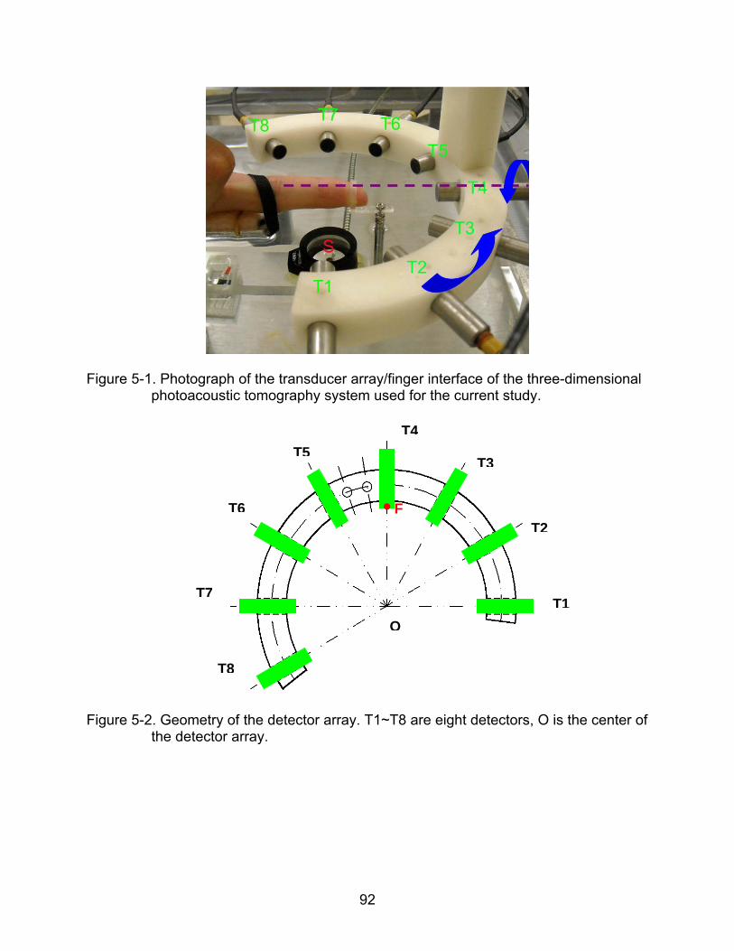
92

Figure 5-1. Photograph of the transducer array/finger interface of the three-dimensional photoacoustic tomography system used for the current study.

Figure 5-2. Geometry of the detector array. T1~T8 are eight detectors, O is the center of the detector array.

O

T1

T2

T3

T4

T5

T6

T7

T8

F

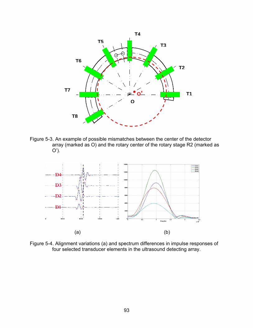
93

Figure 5-3. An example of possible mismatches between the center of the detector array (marked as O) and the rotary center of the rotary stage R2 (marked as O’).

(a) (b)

Figure 5-4. Alignment variations (a) and spectrum differences in impulse responses of four selected transducer elements in the ultrasound detecting array.

O

T1

T2

T3

T4

T5

T6

T7

T8

O’

D1

D2

D3

D4

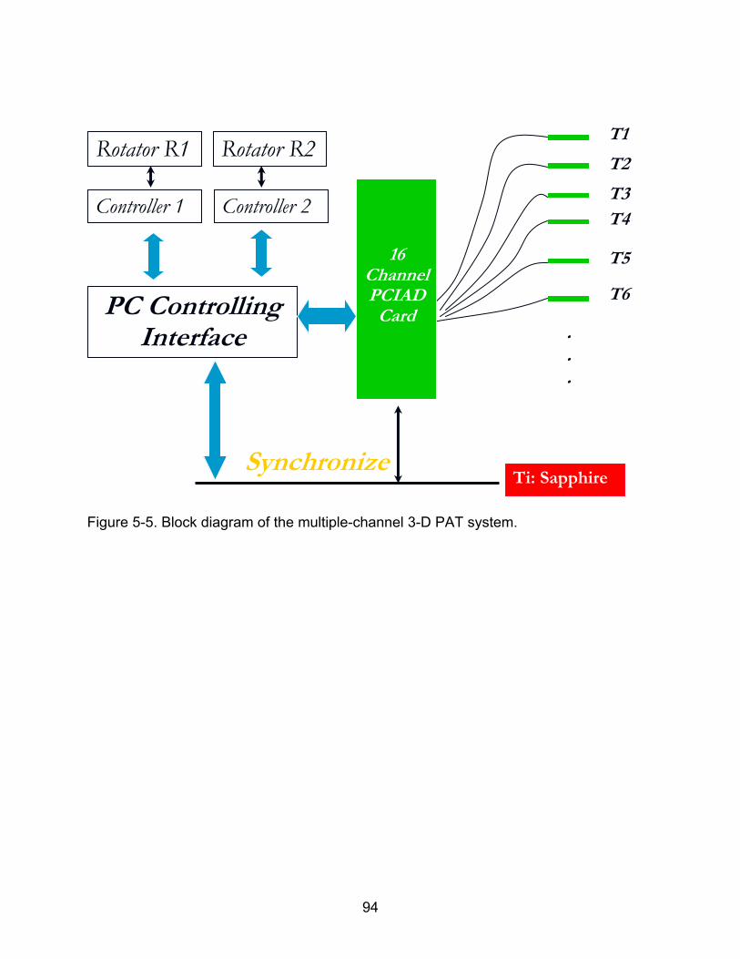
94

Figure 5-5. Block diagram of the multiple-channel 3-D PAT system.

PC Controlling Interface

Rotator R2 Rotator R1

16 ChannelPCIAD

Card

T1

T2

T3 T4

T5

T6

Ti: SapphireSynchronize

.

.

.

Controller 1 Controller 2

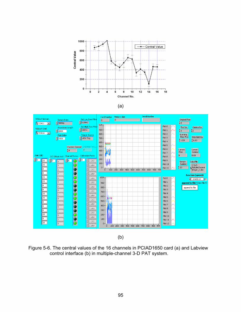
95

(a)

(b)

Figure 5-6. The central values of the 16 channels in PCIAD1650 card (a) and Labview control interface (b) in multiple-channel 3-D PAT system.

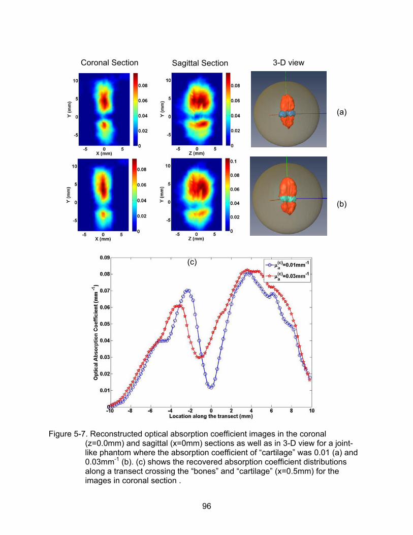
96

Coronal Section

Sagittal Section 3-D view

(a)

(b)

Figure 5-7. Reconstructed optical absorption coefficient images in the coronal

(z=0.0mm) and sagittal (x=0mm) sections as well as in 3-D view for a joint-like phantom where the absorption coefficient of “cartilage” was 0.01 (a) and 0.03mm-1 (b). (c) shows the recovered absorption coefficient distributions along a transect crossing the “bones” and “cartilage” (x=0.5mm) for the images in coronal section .

(c)

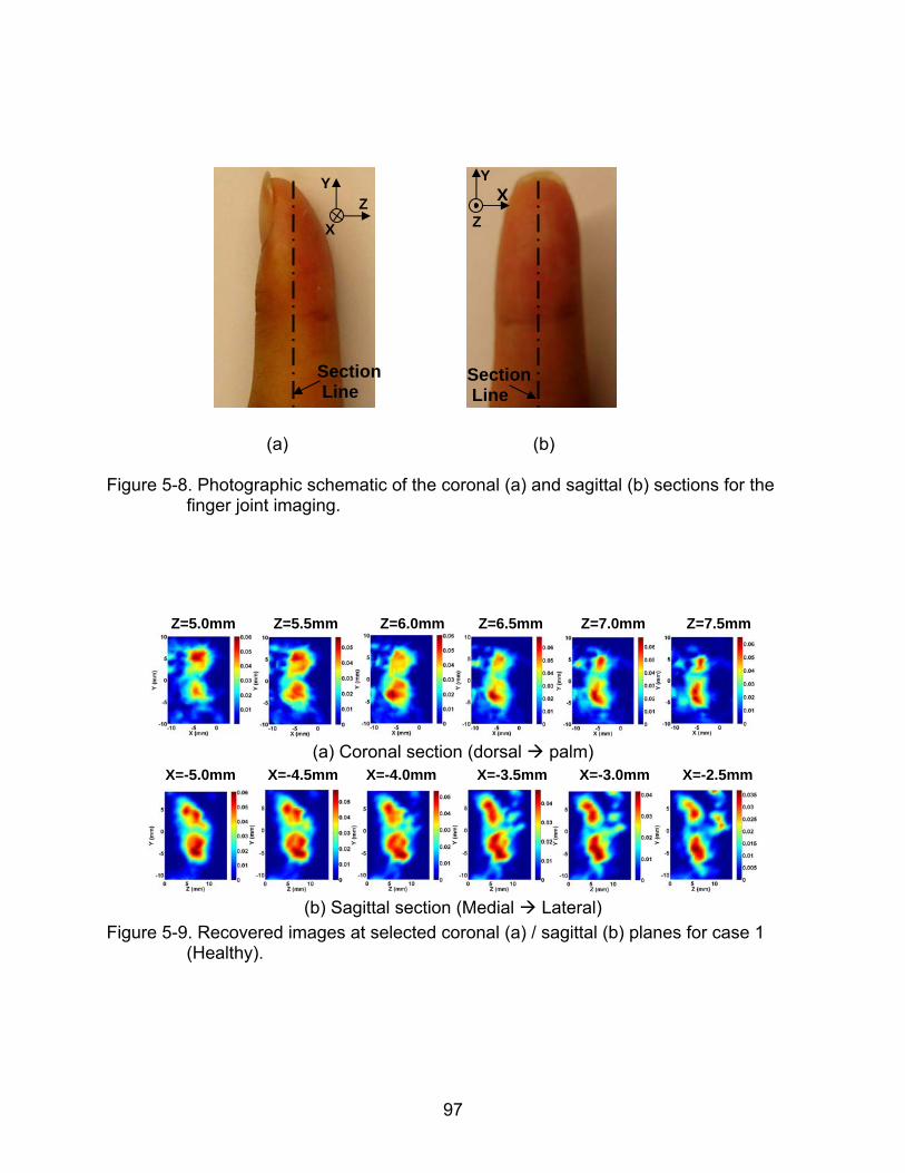
97

(a) (b) Figure 5-8. Photographic schematic of the coronal (a) and sagittal (b) sections for the

finger joint imaging.

Z=5.0mm Z=5.5mm Z=6.0mm Z=6.5mm Z=7.0mm Z=7.5mm

(a) Coronal section (dorsal palm)

X=-5.0mm X=-4.5mm X=-4.0mm X=-3.5mm X=-3.0mm X=-2.5mm

(b) Sagittal section (Medial Lateral)

Figure 5-9. Recovered images at selected coronal (a) / sagittal (b) planes for case 1 (Healthy).

Y Z

X

YX

Z

Section Line

Section Line

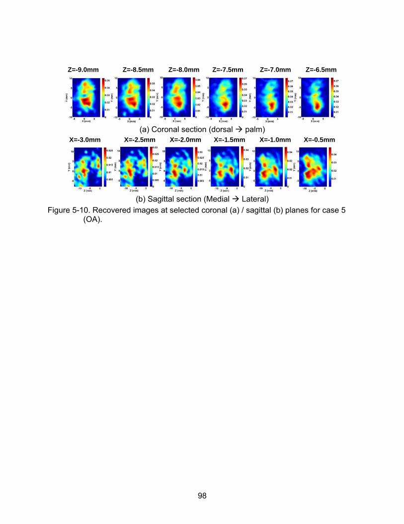
98

Z=-9.0mm Z=-8.5mm Z=-8.0mm Z=-7.5mm Z=-7.0mm Z=-6.5mm

(a) Coronal section (dorsal palm)

X=-3.0mm X=-2.5mm X=-2.0mm X=-1.5mm X=-1.0mm X=-0.5mm

(b) Sagittal section (Medial Lateral)

Figure 5-10. Recovered images at selected coronal (a) / sagittal (b) planes for case 5 (OA).

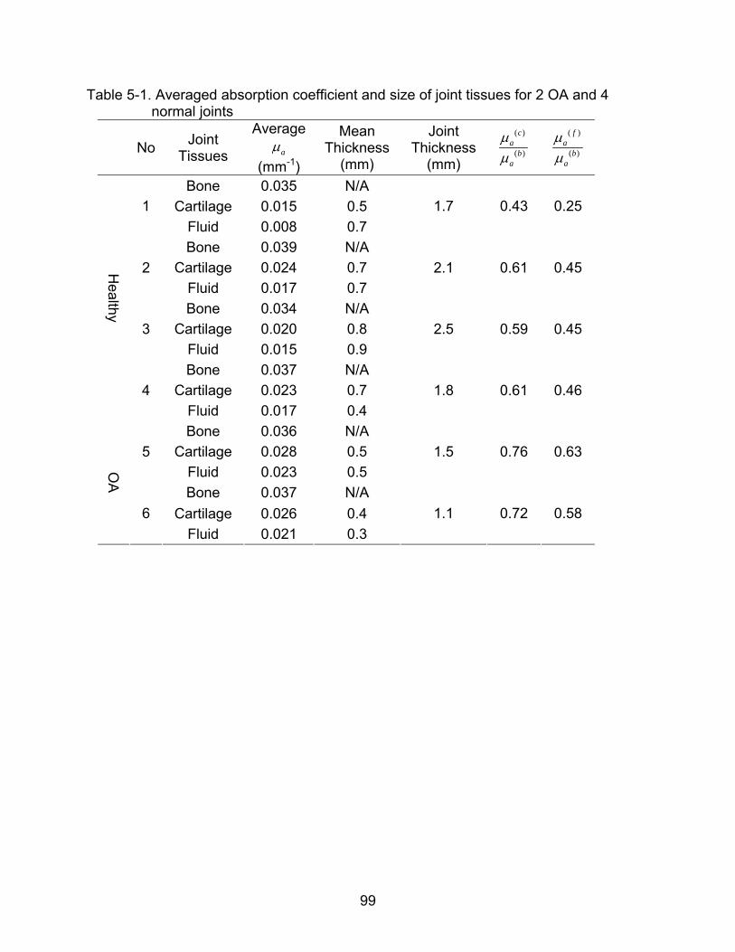
99

Table 5-1. Averaged absorption coefficient and size of joint tissues for 2 OA and 4 normal joints

No Joint

Tissues

Average

a

(mm-1)

Mean Thickness

(mm)

Joint Thickness

(mm)

( )

( )

ca

ba

( )

( )

fa

ba

Bone 0.035 N/A

Cartilage 0.015 0.5 1

Fluid 0.008 0.7

1.7 0.43 0.25

Bone 0.039 N/A

Cartilage 0.024 0.7 2

Fluid 0.017 0.7

2.1 0.61 0.45

Bone 0.034 N/A

Cartilage 0.020 0.8 3

Fluid 0.015 0.9

2.5 0.59 0.45

Bone 0.037 N/A

Cartilage 0.023 0.7

Healthy

4

Fluid 0.017 0.4

1.8 0.61 0.46

Bone 0.036 N/A

Cartilage 0.028 0.5 5

Fluid 0.023 0.5

1.5 0.76 0.63

Bone 0.037 N/A

Cartilage 0.026 0.4

OA

6

Fluid 0.021 0.3

1.1 0.72 0.58

100

CHAPTER 6 IN-VIVO IMAGIING OF CHROMOPHORE CONCENTRATIONS IN FINGER JOINTS

WITH MULTISPECTRAL 3-D PAT

Since last decade, near-infrared spectroscopy and NIR based multispectral

imaging techniques (such as diffuse optical tomography) has emerged as promising

methods to noninvasively image or measure tissue chromophores and associated

hemodynamics in living tissues. In those techniques, concentration distributions of

physiologically / functionally significant tissue chromophores (such as oxy-hemoglobin ,

deoxy-hemoglobin, water, lipid) and their variations due to disease development,

metabolic changes, cerebral hemorrhage, and brain activity can be measured or imaged

by taking the advantage of the absorption spectra of different tissue chromophores.85-94

Thus far, studies has shown that the measurement of these tissue chromophores and

their physiological / functional changes are of great significance both in basic science

(such as neuroscience, molecular imaging of small animals) and clinical applications

(such as breast cancer detection and classification). For example, the concentrations of

oxy-hemoglobin and deoxy-hemoglobin in breast tumors are found to be higher than

normal tissues.96

In recently years, multispectral photoacoustic tomography (PAT) has been

investigated aiming to quantify these same tissue chromophores and the oxygenation

for molecular imaging and functional imaging with high spatial resolution, which can be

as high as sub100 m for several mm penetration depths in highly resolved PAT

images.35-42 Although the challenges remain since the conventional PAT images are the

distributions of absorbed optical energy density and not actual images of the absorption

coefficients that can be immediately ready for quantitative spectroscopic analysis,35

101

several models have been proposed and developed to quantitatively resolve the tissue

chromophores with multispectral PAT.36-40 For example, maps of optical absorption

coefficients can be recovered when the traditional PAT is couple with a photon diffusion

model under certain assumptions, such as pre-known scattering property or wavelength

dependency of the scattering property in the medium. The recovered maps of optical

absorption coefficients in multi-wavelengths further go through spectroscopic analysis

for quantitatively resolved concentrations of the tissue chromophores. Some groups

made further attempts to in-vivo measure the concentrations of oxy-hemoglobin and

deoxy-hemoglobin within blood vessels in a human finger,41 and to image the

hemoglobin and oxygenation in a rat brain,42 although more accurate results require

more accurate models of multispectral PAT.

In this section, our goal is to advance the application of multispectral PAT to in-

vivo imaging of chromophore concentrations in finger joints. Although previous studies

focused on 2-D modeled multispectral PAT, a multispectral 3-D PAT approach is used

in our study, which is more accurate and is essential to capture the full volumetric

structures in high resolved PAT images with less artifacts and blurring than an approach

with 2-D approximation, particularly for tissues with high structural heterogeneity (such

as finger joints). Optical wavelengths from 730nm to 880nm are used in our

multispectral 3-D PAT approach since studies have indicated that multispectral light with

wavelengths located on the two sides of 805nm is required to distinguish the

concentrations of oxy-hemoglobin and deoxy-hemoglobin from the combined optical

absorption values.97

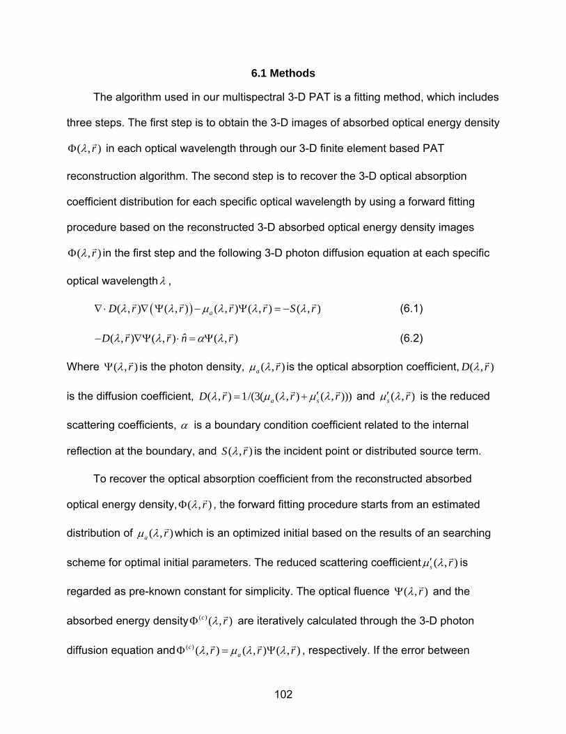
102

6.1 Methods

The algorithm used in our multispectral 3-D PAT is a fitting method, which includes

three steps. The first step is to obtain the 3-D images of absorbed optical energy density

( , )r

in each optical wavelength through our 3-D finite element based PAT

reconstruction algorithm. The second step is to recover the 3-D optical absorption

coefficient distribution for each specific optical wavelength by using a forward fitting

procedure based on the reconstructed 3-D absorbed optical energy density images

( , )r

in the first step and the following 3-D photon diffusion equation at each specific

optical wavelength ,

( , ) ( , ) ( , ) ( , ) ( , )aD r r r r S r

(6.1)

ˆ( , ) ( , ) ( , )D r r n r

(6.2)

Where ( , )r

is the photon density, ( , )a r is the optical absorption coefficient, ( , )D r

is the diffusion coefficient, ( , ) 1/(3( ( , ) ( , )))a sD r r r

and ( , )s r is the reduced

scattering coefficients, is a boundary condition coefficient related to the internal

reflection at the boundary, and ( , )S r is the incident point or distributed source term.

To recover the optical absorption coefficient from the reconstructed absorbed

optical energy density, ( , )r

, the forward fitting procedure starts from an estimated

distribution of ( , )a r which is an optimized initial based on the results of an searching

scheme for optimal initial parameters. The reduced scattering coefficient ( , )s r is

regarded as pre-known constant for simplicity. The optical fluence ( , )r

and the

absorbed energy density ( ) ( , )c r

are iteratively calculated through the 3-D photon

diffusion equation and ( ) ( , ) ( , ) ( , )car r r

, respectively. If the error between

103

( , )r

and ( ) ( , )c r

is not small for a specific optical wavelength, then the

current ( , )a r is updated by ( , ) ( , ) / ( , )a r r r

and the above procedure is

repeated until a small error between ( , )r

and ( ) ( , )c r

is reached, resulting in a

stable quantitative distribution of ( , )a r .

A third step is to recover the concentrations of major tissue chromophores (oxy-

hemoglobin, deoxy-hemoglobin, and water) from the resolved optical absorption

coefficients maps at each wavelength, based on the absorption spectra of these tissue

chromophores and the following Beer’s law in consideration of the optical absorption

contributions from L chromophores.

1

( , ) ( ) ( )L

a i ii

r c r

(6.3)

Where ( )ic r

is the concentration of thi chromophore in the unit of molar ( / )M mole L ;

( )i is the absorption extinction coefficient of the thi chromophore at wavelength . The

chromophores number 2L for the recovery of two tissue chromophores (oxy-

hemoglobin, deoxy-hemoglobin) in our study, which comprise the major contributions to

the optical absorption in the wavelength region we used.

To recover the concentrations of these tissue chromophores, an inverse equation

is used, which is written as the following

ˆ ˆ ˆ( ) ( )aJ J c r J r T TI

(6.4)

Where ˆ ( )ij j iJ ; the elements ( )c r

and ( )a r are ( )jc r

and ( , )a i r

, respectively.

is a regularization factor to stabilize the inverse solution.

104

6.2 In-vivo Experiments

The in-vivo experiments are conducted by our 3-D PAT system described in detail

in Chapter 5, which are comprised of a pulsed NIR light source with wavelength tunable

from 600nm to 950nm, a spherical scanning subsystem, an ultrasound detection array

and associated data acquisition system. Six optical wavelengths from 730nm to 880nm

(730, 760, 805, 825, 850 and 880nm) are chosen for the multispectral 3-D PAT scanner,

which may give the improved distinguishability between HbO2 and Hb. Both the

ultrasound array and the examined finger are immersed in a water tank, which is filled

with warm water, for minimized ultrasound attenuation. During the examination, the

palmar side of the examined DIP finger joint faced up at the center of the two rotary

stages R1 and R2, allowing the finger joint to be illuminated from the dorsal side of the

finger. The collection of the acoustic signals at 360 locations along the spherical

scanning surface surrounding the examined DIP joint requires about 5 minutes in each

wavelength, and the entire procedure of multispectral 3-D photoacoustic examination

lasts for about 30 minutes. Again, the proximal end and the distal end of the examined

finger are secured on the plastic holder to reduce the motion error during the entire in-

vivo examination procedure. To reduce the impact of possible motion errors on our

multispectral PAT, our multispectral 3-D PAT scanner operates in the following

wavelength order: 730nm, 805nm, 850nm, 880nm, 825nm, 760nm. A homemade 3-D

positioning ruler (Figure 6-2) is used to check the location of the examined finger joint

before and after the whole examination procedure, to eliminate failed examinations with

obvious finger motion during the examination procedure.

Seven subjects (two OA patients and five healthy subjects) entered the current

study between 2008 and 2009. All participants (white female; mean age 61 years, range

105

45–71 years) provided informed consent as part of the protocol approved by the

Institutional Review Board of University of Florida. One distal interphalangeal (DIP)

finger joint, joint II at the left hand, from each subject was examined clinically and

photoacoustically in this study, because it was mostly vulnerable to OA disease and at

the same time easily accessible with our current multispectral 3-D PAT scanner. Clinical

examination of each patient was performed independently by a single rheumatologist

(E.S. Sobel). The healthy controls had no known OA or other joint diseases.

Four of the seven recruited subjects (two OA patients and two healthy controls)

completed the whole procedure of 3-D multispectral photoacoustic scanning resulted in

successful photoacoustic image reconstruction and quantitative measurement of oxy-

hemoglobin and deoxy-hemoglobin in our study.

6.3 Results and Discussion

The 3-D photoacoustic images of the DIP joints from all four human subjects were

reconstructed by using a spherical mesh of 7519 finite element nodes and 41323

tetrahedral elements. The optical absorption maps of reconstructed DIP joints are

further recovered under each optical wavelength by coupling reconstructed 3-D

photoacoustic images (deposited optical absorption energy) of the examined DIP joints

with 3-D photon diffusion model. Among the six optical wavelengths where the DIP

joints are reconstructed and their optical absorption maps are quantitatively recovered,

three optical wavelengths are selected, based on the relatively structural consistencies

of the recovered optical absorption maps, for further spectroscopic analysis to

quantitatively resolve the concentrations of HbO2 and Hb.

Figure 6-3(a) and 6-3(b) are the recovered optical absorption maps in coronal

section and sagittal section, respectively, of an in-vivo finger joint at wavelengths from

106

730nm to 880nm. As can be observed in Figure 6-3(a) and 6-3(b), the joint tissue/space

is differentiated from the adjacent bones in the coronal and/or sagittal sections at

several optical wavelengths (760nm, 805nm, 850nm and 880nm). Relatively structural

consistencies of the recovered optical absorption maps are observed between the

wavelengths in 760nm, 805nm and 850nm, which are selected to further quantitatively

resolve the tissue chromophore concentrations. The reason that the joint tissue/space is

missing or fused with the adjacent bones at some optical wavelengths (such as 730nm

and 825nm) are most likely due to motion error during the 30 minutes examination

procedure, although an optimized wavelength order is followed in our 3-D multispectral

PAT scanning. We believe that the motion error and the structural inconsistencies of the

recovered optical absorption maps at some wavelengths can be significantly reduced by

using an ultrasound array integrated with much more ultrasound detectors (for example,

64 detector elements as being used in high resolution whole-body mouse imaging).80

The quantitatively resolved concentrations of HbO2 and Hb from a typical OA

finger joint, which is the same finger joint shown in Figure 6-3, are displayed in Figure 6-

4. The concentrations of HbO2 (Figure 6-4(a)) in different joint tissues are clearly

differentiated in high resolution both in coronal section and sagittal section, and it is

relatively higher in the bones than in the joint cavity. Figure 6-4(b) shows the

concentrations of Hb both in coronal section and sagittal section, where the joint cavity

is differentiated from the adjacent phalanges in the sagittal section and is barely

identifiable in the coronal section. We believe that the relatively poor quality of the

resolved Hb concentration images in coronal section is most likely due to the relatively

low quality image at the wavelength 760nm, where the absorption spectrum of Hb has a

107

high peak and motion error may have happened during the 3-D multispectral PAT

scanning.

Figure 6-5 shows the quantitatively resolved concentrations of HbO2 and Hb from

a typical healthy finger joint. Again, the structure of joint space is clearly identified in the

images of each resolved chromophore, and the concentrations of HbO2 and Hb in the

joint cavity are found to be relatively lower than that in the adjacent phalanges. In

comparison with the OA finger joint shown in Figure 6-4, the joint cavity in healthy

subjects seems more distinctive.

For all the four examined in-vivo finger joints, the average concentrations of oxy-

hemoglobin (HbO2), totoal hemoglobin (Total-Hb) and the oxygen saturation (SO2) and

H2O) in the joint cavity and the adjacent bones are calculated and presented in Figure

6-6. As can be observed from Figure 6-6(a), the average concentrations of HbO2 and

Total-Hb in the finger phalanges are in the range from 44 to 58 M , and from 68 to

96 M , respectively. The quantitatively resolved concentration levels of HbO2 and

Total-Hb are in agreement with the measurements by diffuse near-Infrared

spectroscopy. 98 Further observations indicate a difference in the levels of total-Hb

between finger phalanges with OA disease and healthy phalanges, which are in range

of 86 ~ 96 M and 68 ~ 69 M , respectively. The finding of enhanced hemoglobin levels

in OA joints has the pathologic roots revealed by previous studies, where angiogenesis

has been observed in diseased tissues. The oxygen saturations of the four in-vivo

finger joints are observed from 58% to 66% in the finger phalanges, while finger

phalanges with OA disease seems to have lower oxygen saturations levels (55%~60%)

than healthy phalanges (65%~66%). Hypoxia in osteoarthritic phalanges has been

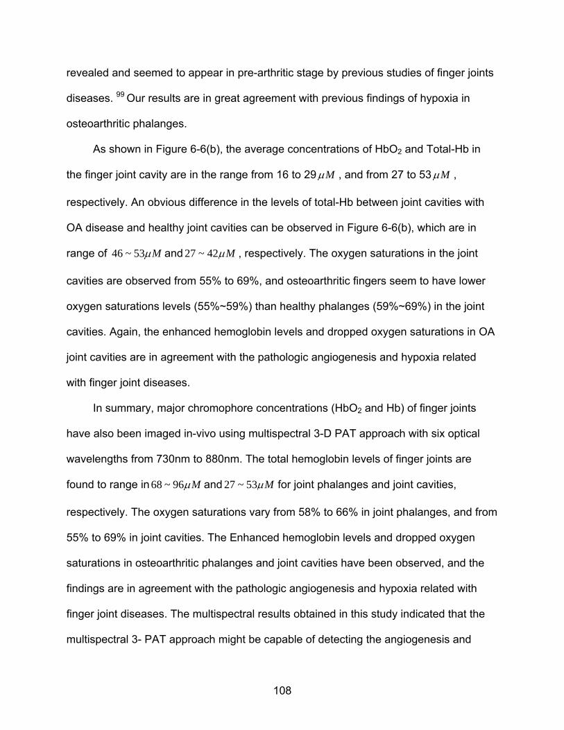
108

revealed and seemed to appear in pre-arthritic stage by previous studies of finger joints

diseases. 99 Our results are in great agreement with previous findings of hypoxia in

osteoarthritic phalanges.

As shown in Figure 6-6(b), the average concentrations of HbO2 and Total-Hb in

the finger joint cavity are in the range from 16 to 29 M , and from 27 to 53 M ,

respectively. An obvious difference in the levels of total-Hb between joint cavities with

OA disease and healthy joint cavities can be observed in Figure 6-6(b), which are in

range of 46 ~ 53 M and 27 ~ 42 M , respectively. The oxygen saturations in the joint

cavities are observed from 55% to 69%, and osteoarthritic fingers seem to have lower

oxygen saturations levels (55%~59%) than healthy phalanges (59%~69%) in the joint

cavities. Again, the enhanced hemoglobin levels and dropped oxygen saturations in OA

joint cavities are in agreement with the pathologic angiogenesis and hypoxia related

with finger joint diseases.

In summary, major chromophore concentrations (HbO2 and Hb) of finger joints

have also been imaged in-vivo using multispectral 3-D PAT approach with six optical

wavelengths from 730nm to 880nm. The total hemoglobin levels of finger joints are

found to range in 68 ~ 96 M and 27 ~ 53 M for joint phalanges and joint cavities,

respectively. The oxygen saturations vary from 58% to 66% in joint phalanges, and from

55% to 69% in joint cavities. The Enhanced hemoglobin levels and dropped oxygen

saturations in osteoarthritic phalanges and joint cavities have been observed, and the

findings are in agreement with the pathologic angiogenesis and hypoxia related with

finger joint diseases. The multispectral results obtained in this study indicated that the

multispectral 3- PAT approach might be capable of detecting the angiogenesis and

109

hypoxia in pre-arthritic stage of OA disease, and is promising as a potential clinical tool

for early detection OA in the finger joints.

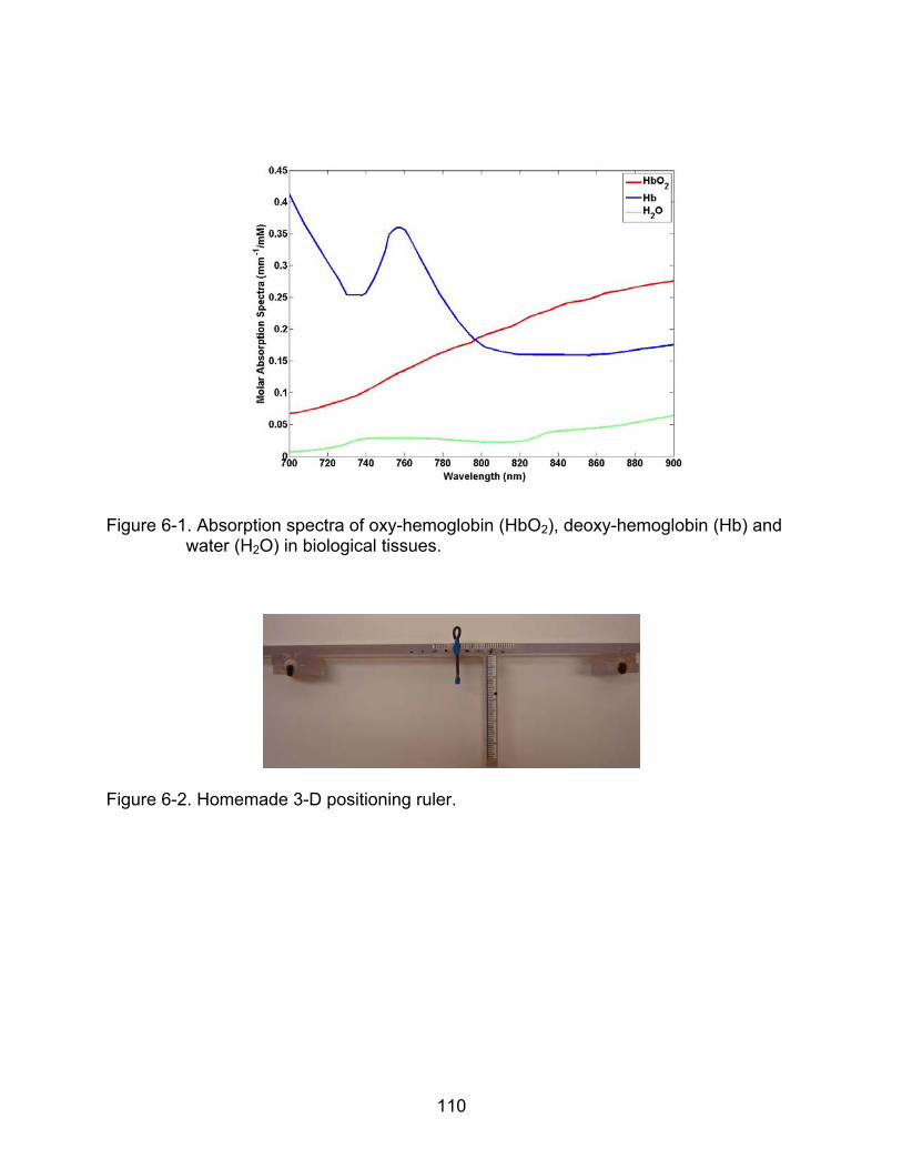
110

Figure 6-1. Absorption spectra of oxy-hemoglobin (HbO2), deoxy-hemoglobin (Hb) and water (H2O) in biological tissues.

Figure 6-2. Homemade 3-D positioning ruler.

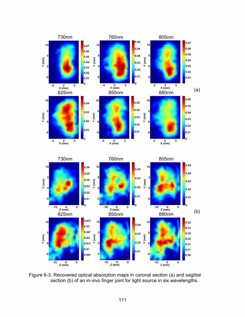
111

730nm

760nm 805nm

825nm

850nm 880nm (a)

730nm

760nm 805nm

825nm 850nm 880nm (b)

Figure 6-3. Recovered optical absorption maps in coronal section (a) and sagittal

section (b) of an in-vivo finger joint for light source in six wavelengths.

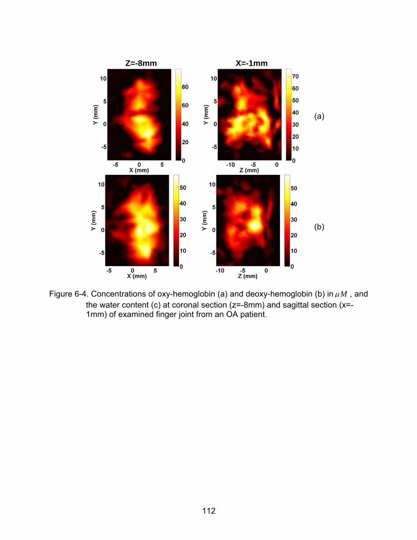
112

Z=-8mm

X=-1mm

(a)

(b)

Figure 6-4. Concentrations of oxy-hemoglobin (a) and deoxy-hemoglobin (b) in M , and

the water content (c) at coronal section (z=-8mm) and sagittal section (x=-1mm) of examined finger joint from an OA patient.

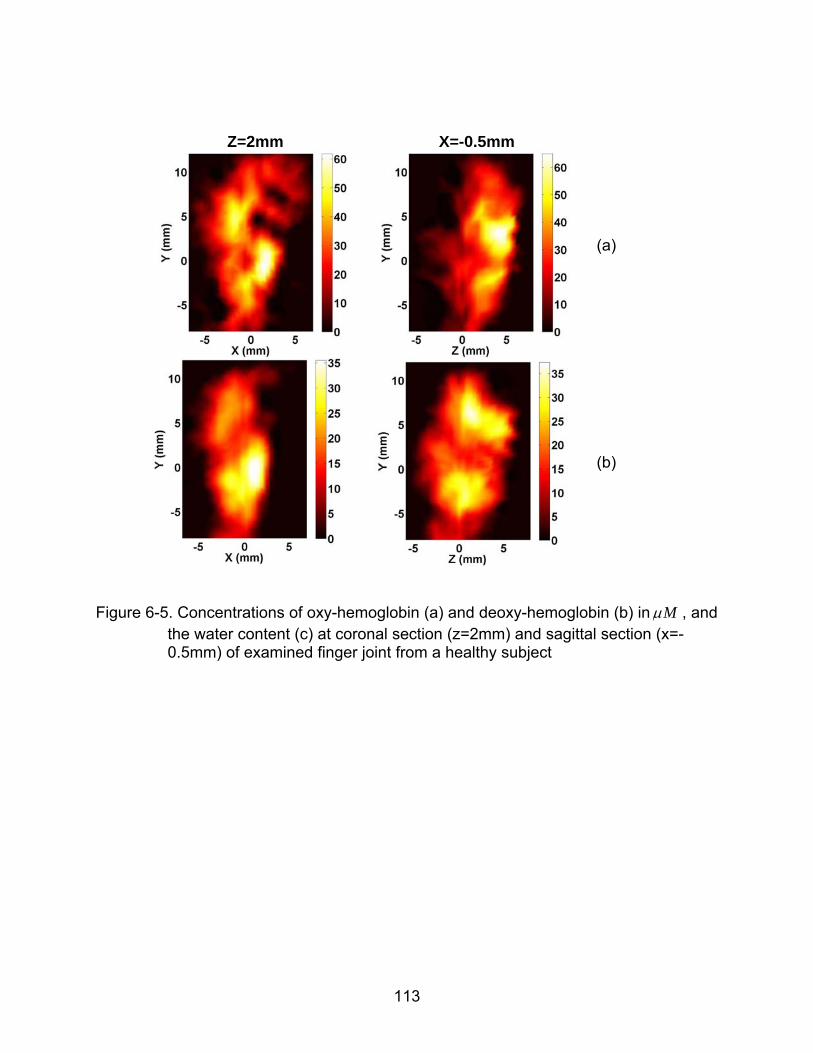
113

Z=2mm

X=-0.5mm

(a)

(b)

Figure 6-5. Concentrations of oxy-hemoglobin (a) and deoxy-hemoglobin (b) in M , and

the water content (c) at coronal section (z=2mm) and sagittal section (x=-0.5mm) of examined finger joint from a healthy subject

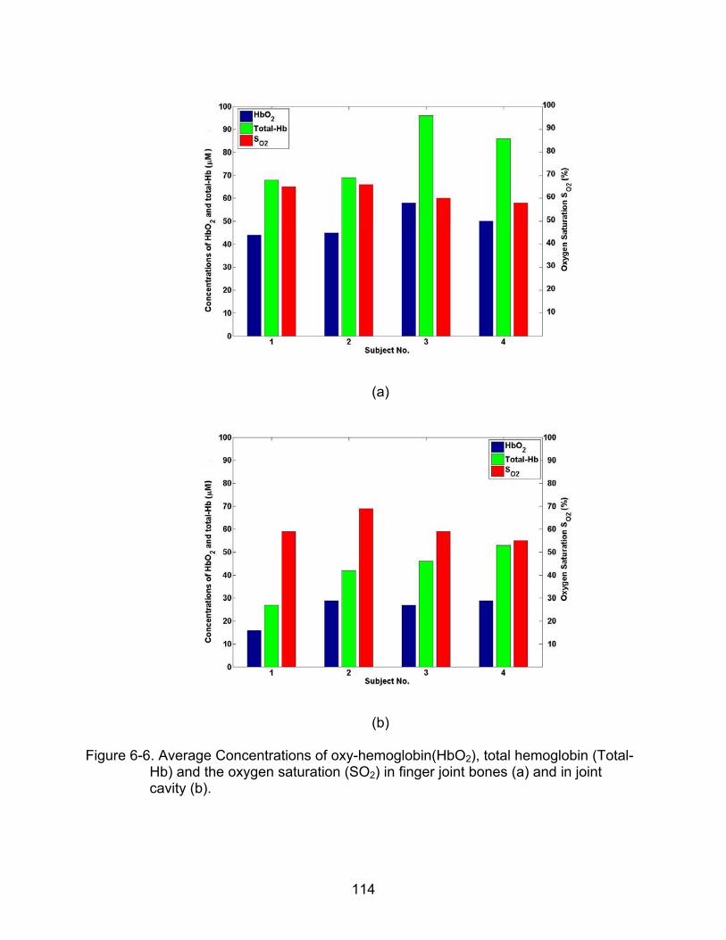
114

(a)

(b)

Figure 6-6. Average Concentrations of oxy-hemoglobin(HbO2), total hemoglobin (Total-Hb) and the oxygen saturation (SO2) in finger joint bones (a) and in joint cavity (b).

115

CHAPTER 7 CONCLUSION AND FUTHER WORK

7.1 Conclusion

In this dissertation, we have investigated the feasibilities of 3-D PAT approach to

image in-vivo finger joints and to detect the OA disease in the hand. Also multispectral

3-D PAT is studied to measure the major tissue chromophore concentrations (HbO2, Hb

and H2O) of in-vivo finger joints.

Results based on finger-like phantom experiments, in-vivo finger joint imaging and

clinical cases study show that 3-D PAT in a spherical scanning geometry is able to

image in-vivo finger joints in high resolution and is promising to detect the finger OA in

the hand. Major anatomical structures of an examined distal interphalangeal (DIP) joint

along with the side arteries are clearly imaged, where joint space is well differentiated

from surrounding finger phalanges. Seven subjects enrolled in our study are

photoacoustically examined with our 8-channel 3-D PAT system, and apparent

differences, in both the reconstructed size of the joint space and the absorption

coefficient of the joint cavity, are observed between OA and normal joints. Major

chromophore concentrations (HbO2, Hb) of in-vivo finger joints are quantitatively imaged

by using 3-D multispectral PAT approach with six optical wavelengths from 730nm to

880nm, and the quantitative results are consistent with previous studies.

As our studies indicate, the parallel computing technique, 3-D PAT approach in a

spherical scanning geometry, efficient optical lighting method and calibrated multiple

ultrasound detecting system are essential for effective finger joints reconstruction, OA

detection and chromophores recovery. An ultrasound detecting system with much more

detectors is expected to further improve the images quality and quantitative results.

116

Although the image quality (in terms of spatial resolution) provided by our 3-D PAT

seems not comparable to MRI, our 3-D PAT is able to obtain optical absorption

coefficient and physiological / functional information of the joint tissues (cartilage, fluid,

phalanges, etc) in higher spatial resolution over pure optical techniques. In addition,

PAT is portable and low in cost. While our current 3-D PAT approach is not optimized, it

allows us to demonstrate the possibility of 3-D in in-vivo finger joint imaging and clinical

cases study of osteoarthritis for the first time, which suggests the possibility of 3-D PAT

as a potential clinical tool for early detection of OA in the finger joints.

7.2 Future Studies

7.2.1 Evaluation of 3-D PAT in OA Detection with Small Clinical Samples

The ultimate goal of this dissertation and our study is to detect OA joints from

normal joints at an early stage. The advancement of the 3-D PAT both in the hardware

and algorithms introduced in this dissertation serve the goal, and studies on limited

clinical OA cases have already indicated that it is promising to detect the finger

osteoarthritis in the hand by imaging abnormal rise of the optical absorption coefficients

in joint cavity (cartilage and synovial fluid) and the narrowing of the joint space with3-D

PAT. However further evaluation with small clinical samples plays a key role to validate

our methods, where the specificity and sensitivity of the 3-D PAT in the detection of OA

patients will be investigated.

7.2.2 In-vivo Detection of Rheumatoid Arthritis in the Hand

Rheumatoid arthritis is another common joint disease, which is characterized as

inflamed joint. Although the 3-D PAT is initially developed to image DIP joint for

detection of OA disease in the hand, it is adjustable for PIP joint imaging and RA

disease detection in the hand. Compared to the DIP joint imaging, PIP joint imaging

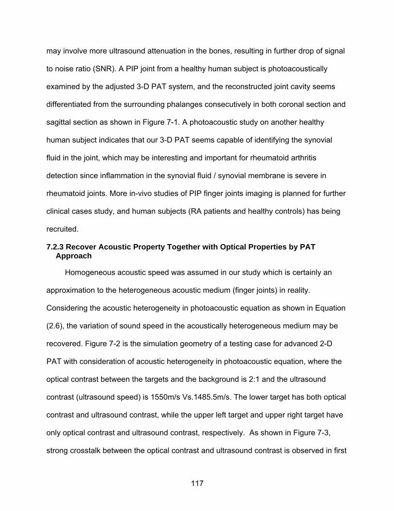
117

may involve more ultrasound attenuation in the bones, resulting in further drop of signal

to noise ratio (SNR). A PIP joint from a healthy human subject is photoacoustically

examined by the adjusted 3-D PAT system, and the reconstructed joint cavity seems

differentiated from the surrounding phalanges consecutively in both coronal section and

sagittal section as shown in Figure 7-1. A photoacoustic study on another healthy

human subject indicates that our 3-D PAT seems capable of identifying the synovial

fluid in the joint, which may be interesting and important for rheumatoid arthritis

detection since inflammation in the synovial fluid / synovial membrane is severe in

rheumatoid joints. More in-vivo studies of PIP finger joints imaging is planned for further

clinical cases study, and human subjects (RA patients and healthy controls) has being

recruited.

7.2.3 Recover Acoustic Property Together with Optical Properties by PAT Approach

Homogeneous acoustic speed was assumed in our study which is certainly an

approximation to the heterogeneous acoustic medium (finger joints) in reality.

Considering the acoustic heterogeneity in photoacoustic equation as shown in Equation

(2.6), the variation of sound speed in the acoustically heterogeneous medium may be

recovered. Figure 7-2 is the simulation geometry of a testing case for advanced 2-D

PAT with consideration of acoustic heterogeneity in photoacoustic equation, where the

optical contrast between the targets and the background is 2:1 and the ultrasound

contrast (ultrasound speed) is 1550m/s Vs.1485.5m/s. The lower target has both optical

contrast and ultrasound contrast, while the upper left target and upper right target have

only optical contrast and ultrasound contrast, respectively. As shown in Figure 7-3,

strong crosstalk between the optical contrast and ultrasound contrast is observed in first

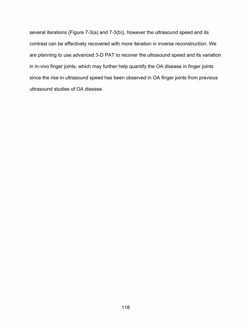
118

several iterations (Figure 7-3(a) and 7-3(b)), however the ultrasound speed and its

contrast can be effectively recovered with more iteration in inverse reconstruction. We

are planning to use advanced 3-D PAT to recover the ultrasound speed and its variation

in in-vivo finger joints, which may further help quantify the OA disease in finger joints

since the rise in ultrasound speed has been observed in OA finger joints from previous

ultrasound studies of OA disease.

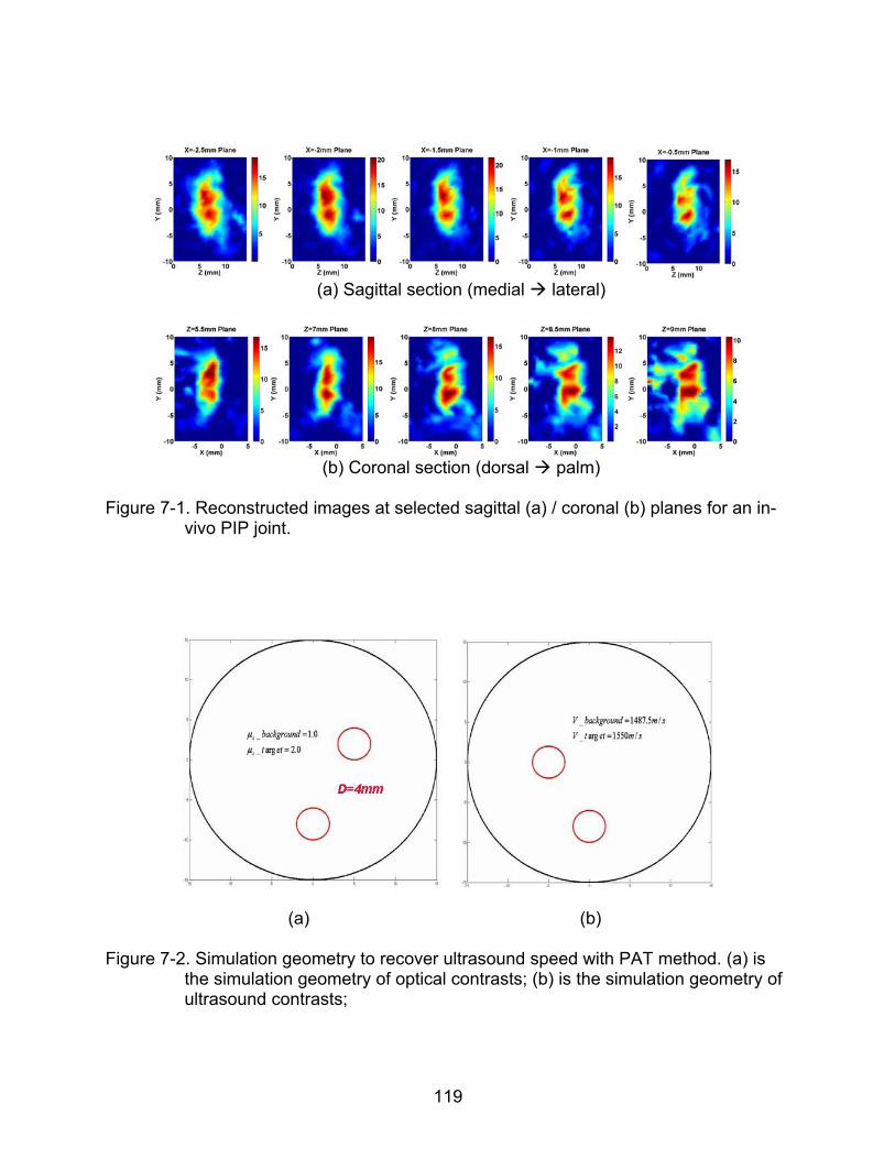
119

(a) Sagittal section (medial lateral)

(b) Coronal section (dorsal palm)

Figure 7-1. Reconstructed images at selected sagittal (a) / coronal (b) planes for an in-

vivo PIP joint.

(a) (b)

Figure 7-2. Simulation geometry to recover ultrasound speed with PAT method. (a) is the simulation geometry of optical contrasts; (b) is the simulation geometry of ultrasound contrasts;

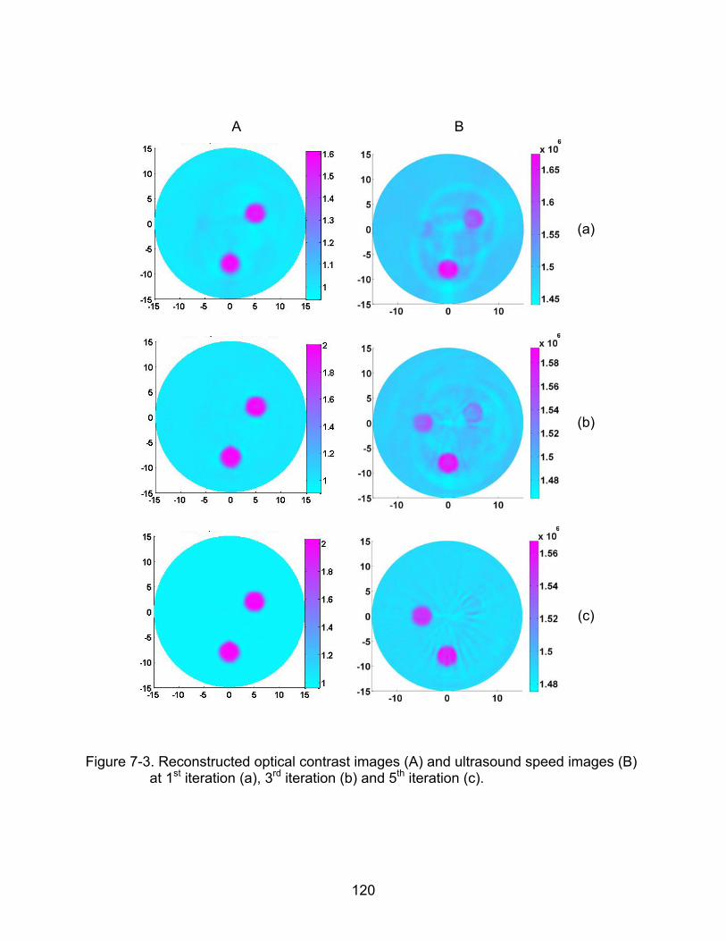
120

A B

(a)

(b)

(c)

Figure 7-3. Reconstructed optical contrast images (A) and ultrasound speed images (B) at 1st iteration (a), 3rd iteration (b) and 5th iteration (c).

121

LIST OF REFERENCES

1. H. Jiang, N. Iftimia, Y. Xu, J. Eggert, L. Fajardo, and K. Klove, “Near-infrared optical imaging of the breast with model-based reconstruction,” Acad. Radiol. 9, 186–194 (2002).

2. X. Gu, Q. Zhang, M. Bartlett, L. Schutz, L. Fajardo, and H. Jiang, “Differentiation of cysts from solid tumors in the breast with diffuse optical tomography,” Acad. Radiol. 11, 53–60 (2004).

3. A. E. Cerussi, A. Berger, F. Bevilacqua, N. Shah, D. Jakubowski, J. Butler, R. Holcombe, and B. Tromberg, “Sources of absorption and scattering contrast for nearinfrared optical mammography,” Acad. Radiol. 8, 211–218 (2001).

4. A. H. Hielscher, A. D. Klose, A. K. Scheel, B. Moa-Anderson, M. Backhaus, U. J. Netz, et al, “Sagittal laser optical tomography for imaging of rheumatoid finger joints,” Phys. Med. Biol. 49, 1147–1163 (2004).

5. A. Pifferi, A. Torricelli, P. Taroni, A. Bassi, E. Chikoidze, E. Giambattistelli, “Optical biopsy of bone tissue: a step toward the diagnosis of bone pathologies,” J. Biomed. Opt. 9, 474–480 (2004).

6. Z. Yuan, Q. Zhang, H. Jiang, “3D diffuse optical tomography imaging of osteoarthritis: Initial results in finger joints,” J. Biomed. Opt. 12, 034001 (2007).

7. A. K. Scheel, M. Backhaus, A. D. Klose, B. Moa-Anderson, U. J. Netz, K. G. Hermann, et al, “First clinical evaluation of sagittal laser optical tomography for detection of synovitis in arthritic finger joints,” Ann. Rheum. Dis. 64, 239–245 (2005).

8. A. A. Oraevsky, A. A. Karabutov and S. V. Solomatin, “Laser optoacoustic imaging of breast cancer in vivo,” Proc. SPIE 4526, 6–11 (2001).

9. S. Manohar, A. Kharine, J. C. G. van Hespen, W. Steenbergen and T. G. van Leeuwen, “Photoacoustic mammography laboratory prototype: imaging of breast tissue phantoms,” Phys. Med. Biol. 50, 2543–2557(2005).

10. R. G. M. Kollkman, J. H. G. M. Klaessens, E. Hondebrink, J. C. W. Hopman, F. F. M. de Mul, W. Steenbergen, J. M. Thijssen and T. G. V. Leeuwen, “Photoacoustic determination of blood vessel diameter,” Phys. Med. Biol. 49, 4745–4756(2004).

11. R. I. Siphanto, K. K. Thumma, R. G. M. Kolkman, T. G. van Leeuwen, F. F. M. de mul, J.W. van Neck, L.N.A. van Adrichem, and W. Steenbergen, “Serial noninvasive photoacoustic imaging of neovascularization in tumor angiogenesis,” Opt. Express 13, 8995 (2005).

12. S. Yang, D. Xing, Q. Zhou, L. Xiang and Y. Lao, “Functional imaging of cerebrovascular activities in small animals using high-resolution photoacoustic tomography,” Med. Phys. 34, 3294–3301 (2007).

13. X. Wang, Y. Pang, G. Ku, X. Xie, G. Stoica, and L. V. Wang, “Noninvasive laser-induced photoacoustic tomography for structural and functional in vivo imaging of the brain,” Nat. Biotechnol. 21, 803–806 (2003).

122

14. E. Z. Zhang, J. Laufer and P. Beard, “Three dimensional photoacoustic imaging of vascular anatomy in small animals using an optical detection system,” Proc. SPIE 6437, 643710S (2007).

15. A. A. Karabutov, E. Savateeva, A. Oraevsky, “Imaging of layered structures in biological tissues with opto-acoustic front surface transducer,” Proc. SPIE 3601, 284–295 (1999).

16. C. G. A. Hoelen, F. F. M. de Mul, R. Pongers, and A. Dekker, “Three-dimensional photoacoustic imaging of blood vessels in tissue,” Opt. Lett. 23, 648–650 (1998).

17. J. A. Viator, G. Au, G. Paltauf, S. Jacques, S. Prahl, H. Ren, Z. Chen, J. Nelson, “Clinical testing of a photoacoustic probe for port wine stain depth determination,” Lasers Surg. Med. 30, 141–148 (2002).

18. S. Y. Emelianov, P. Li and M. O’Donnell, “Photoacoustics for molecular imaging and therapy,” Phys. Today. 05, 34–39 (2009).

19. D. Razansky, M. Distel, C. Vinegoni, R. Ma, N. Perrimon, R. W. Ko¨ster and V. Ntziachristos, “Multispectral opto-acoustic tomography of deep-seated fluorescent proteins in vivo,” Nat. Photonics 3, 379–379 (2009).

20. H. F. Zhang, K. Maslov, G. Stoica and L. V. Wang, “Functional photoacoustic microscopy for high-resolution and noninvasive in vivo imaging,” Nat. Biotechnol. 24, 848–851 (2006).

21. H. F. Zhang, K. Maslov, G. Stoica and L. V. Wang, “In vivo imaging of subcutaneous structures using functional photoacoustic microscopy,” Nat. Protoc. 2, 797–804 (2007).

22. A. D. L. Zerda, C. Zavaleta, S. Keren, et al., ”Carbon nanotubes as photoacoustic molecular imaging agents in living mice,” Nat. Nanotechnol. 3, 557–562 (2008).

23. L. S. Boucharda, M. S. Anwarb, G. L. Liu, et al., ”Picomolar sensitivity MRI and photoacoustic imaging of cobalt nanoparticles,” PNAS 106, 4085–4089 (2009).

24. Q. Zhang, Z. Liu, P. R. Carney, Z. Yuan, H. Chen, S. N Roper and H. Jiang, “Non-invasive imaging of epileptic seizures in vivo using photoacoustic tomography,” Phys. Med. Biol. 53, 1921–1931 (2008).

25. X. Wang, D. L. Chamberland, D. A. Jamadar, “Noninvasive photoacoustic tomography of human peripheral joints toward diagnosis of inflammatory arthritis,” Opt. Lett. 32, 3002–3004 (2007).

26. D. L. Chamberland, X. Wang, B. J. Roessler, “Photoacoustic tomography of carrageenan-induced arthritis in a rat model,” J. Biomed. Opt. 13, 011005 (2008).

27. D. L. Chamberland, A. Agarwal, N. Kotov, J. B. Fowlkes, P. L Carson and X. Wang, “Photoacoustic tomography of joints aided by an Etanercept-conjugated gold nanoparticle contrast agent-an ex vivo preliminary rat study,” Nanotechnology 19, 095101 (2008).

28. J. Ripoll, V. Ntziachristos, “Quantitative point source photoacoustic inversion formulas for scattering and absorbing medium,” Phys. Rev. E 71, 031912 (2005).

123

29. Z. Yuan, H. Jiang, “Quantitative photoacoustic tomography: recovery of optical absorption coefficient map of heterogeneous medium,” Appl. Phys. Lett. 88, 231101 (2006).

30. B. Cox, S. Arridge, K. Kostli and P. Beard, “2D quantitative photoacoustic image reconstruction of absorption distributions in scattering medium using a simple iterative method,” Appl. Opt. 45, 1866–1875 (2006).

31. L. Yao, Y. Sun, and H. Jiang, “Quantitative photoacoustic tomography based on the radiative transfer equation,” Opt. Lett. 34, 1765–1767 (2009).

32. L. Yin, Q. Wang, Q. Zhang, H. Jiang, “ Tomographic imaging of absolute optical absorption coefficient in turbid medium using combing photoacoustic and diffusing light measurements,” Opt. Lett. 32, 2556–2558 (2007).

33. L. Yao, Y. Sun, and H. Jiang, “Transport-based quantitative photoacoustic tomography: Simulations and experiments,” Phys. Med. Biol. 55, 1917–1934 (2010).

34. Z. Yuan, Q. Wang, H. Jiang, “Reconstruction of optical absorption coefficient maps of heterogeneous media by photoacoustic tomography coupled with diffusion equation based regularized Newton Method,” Opt. Express 15, 18076–18081 (2007).

35. B. T. Cox, J. G. Laufer and P. C. Beard, “The challenges for quantitative photoacoustic imaging,” Proc. SPIE 717713, 717713–1–9 (2009).

36. J. Laufer, D. Delpy, C. Elwell and P. Beard, “Quantitative spatially resolved measurement of tissue chromophore concentrations using photoacoustic spectroscopy: application to the measurement of blood oxygenation and haemoglobin concentration,” Phys. Med. Biol. 52, 141–168 (2007).

37. B. T. Cox, S. R. Arridge, and P. C. Beard, “Estimating chromophore distributions from multiwavelength photoacoustic images,” J. Opt. Soc. Am. A 26, 443–455 (2009).

38. Z. Yuan and H. Jiang, “Simultaneous recovery of tissue physiological and acoustic properties and the criteria for heterogeneous media by quantitative photoacoustic tomography,” Opt. Lett. 34, 1714–1716 (2009).

39. Z. Yuan and H. Jiang, “Quantitative photoacoustic tomography,” Phil. Trans. R. Soc. A 367, 3043–3054 (2009).

40. J. Laufer, B. Cox, E. Zhang, and P. Beard, “Quantitative determination of chromophore concentrations from 2D photoacoustic images using a nonlinear model-based inversion scheme,” Appl. Opt. 10, 1219–1233 (2010).

41. J. Laufer, E. Zhang, P. Beard, “Quantitative in vivo measurements of blood oxygen saturation using multiwavelength photoacoustic imaging,” Proc. SPIE 6437, 64371Z–1–9 (2007).

42. X. Wang, X. Xie, G. Ku, and L. V. Wang, “Noninvasive imaging of hemoglobin concentration and oxygenation in the rat brain using high-resolution photoacoustic tomography,” J. Biomed. Opt. 11, 024015–1–9 (2006).

124

43. C. V. Oddis, “New Perspective on Osteoarthritis,” Am. J. Med. 100 2A, 10S–15S (1996).

44. R. W. Moskowitz, R. D. Altman, M. C. Hochberg, J. A. Buchwalter, V. M. Goldberg, “Osteoarthritis: diagnose and medical/surgical management,” Lippincott Williams & Wilkins, Philadelphia, USA (2007).

45. P. Sarzi-Puttini, M. A. Cimmino, R. Scarpa, R. Caporali, F. Parazzini, A. Zaninelli, et al, “Osteoarthritis: an overview of the disease and its treatment strategies,” Semin. Arthritis. Rheum. 35, 1–10 (2005).

46. S. B. Abramson, M. Attur, Y. Yazici, ”Prospect for disease modification in osteoarthritis,” Nat. Clin. Prat. Rheumatol. 2, 304–312 (2006).

47. P. Peloschek, G. Langs, M. Weber, J. Sailer, M. Reisegger, H. Imhof, H. Bischol, F. Kainberger, “An automatic model-based system for joint space measurements on hand radiographs: Initial experience,” Radiology 243, 855–862 (2007).

48. J. T. Sharp, “Assessment of radiographic abnormalities in rheumatoid arthritis: what have we accomplished and where should we go from here,” J. Rheumatol. 22, 1787–1791 (1995).

49. T. Nishii, H. Tanaka, N. Sugano, H. Miki, M. Takao, H. Yoshikawa, “Disorders of acetabular labrum and articular cartilage in hip hysplasia: evaluation using isotropic high-resolution CT arthrography with sequential radial reformation,” Osteoarthritis. Cart. 15, 251–57 (2007).

50. H. I. Keen, R. J. Wakefield, A. J. Grainger, E. M. A. Hensor, P. Emery, P. G. Conaghan, “An Ultrasonographic Study of Osteoarthritis of the Hand: Synovitis and Its Relationship to Structural Pathology and Symptoms,” Arthritis. and Rheumatism. 59, 1756–1763 (2008).

51. J. Chao and K. Kalunian, “Ultrasonography in osteoarthritis: recent advances and prospects for the future,” Current Opinion in Rheumatology 20, 560–564 (2008).

52. J. A. Tyler, P. J. Watson, H. L. Herrod, M. Robson, L. D. Hall, “Detection and monitoring of progressive cartilage degenerationof osteoarthritic cartilage by MRI,” Acta. Orthoped. Scand. Suppl 266, 130–138 (1995).

53. H. Sugimoto, A. Takeda, K. Hyodoh, “Early-stage rheumatoid arthritis: Prospective study of the effectiveness of MR imaging for diagnosis,” Radiology 216, 569–575 (2000).

54. H. Sugimoto, A. Takeda, J. Masuyama, M. Furuse, “Early-stage rheumatoid arthritis: diagnostic accuracy of MR imaging,” Radiology 198, 185–192 (1996).

55. Z. Yuan, Q. Zhang, E. Sobel, H. Jiang, ”Tomographic x-ray guided three-dimensional diffuse optical tomography of osteoarthritis in the finger joints,” J. Biomed. Opt. 13, 044006 (2008).

56. Y. Sun, and H. Jiang, “Quantitative three-dimensional photoacoustic tomography of the finger joints: Phantom studies in a spherical scanning geometry,” Phys. Med. Biol. 54, 5457-5467 (2009)

125

57. Y. Sun, E. Sobel and H. Jiang, “Quantitative three-dimensional photoacoustic tomography of the finger joints: an in-vivo study,” J. Biomed. Opt. 14, 064002–1–5 (2009).

58. Y. Sun, E. Sobel and H. Jiang, “First assessment of three-dimensional quantitative photoacoustic tomography for in vivo detection of osteoarthritis in the finger joints,” Radiology (under review).

59. Y. Sun, E. Sobel and H. Jiang, “In vivo imaging of chromophore concentrations in finger joints by three-dimensional multispectral photoacoustic tomography,” Opt. Exp. (under submission).

60. K. P. Kostli, M. Frenz, H. Bebie, and H. P. Weber, “Temporal backward projection of optoacoustic pressure transients using Fourier transform methods,” Phys. Med. Biol. 46, 1863–1872 (2001).

61. C. G. A. Hoelen, F. F. de Mul, R. Pongers, and A. Dekker, “Three dimensional photoacoustic imaging of blood vessels in tissue,” Opt. Lett. 23, 648–650 (1998).

62. P. Y. Liu, “The P-transform and photoacoustic image reconstruction,” Phys. Med. Biol. 43, 667–674 (1998).

63. Y. V. Zhulina, “Optical statistical approach to optoacoustic image reconstruction,” Appl. Opt. 39, 5971–5977 (2000).

64. K. P. Kostli, D. Frauchiger, J. Niederhauser, G. Paltauf, H. Weber, and M. Frenz, “Optoacoustic imaging using a three-dimensional reconstruction algorithm,” IEEE J. Sel. Top. Quantum Electron. 7, 918–923 (2001).

65. H. Jiang, Z. Yuan, and X. Gu, “Spatially varying optical and acoustic property reconstruction using finite-element-based photoacoustic tomography,” J. Opt. Soc. Am. A. 23, 878–888 (2006).

66. Z. Yuan, Q. Zhang, H. Jiang, “Simultaneous reconstruction of acoustic and optical properties of heterogeneous media by quantitative photoacoustic tomography,” Opt. Exp. 14, 6749–6754 (2006).

67. Z. Yuan and H. Jiang, “Three-dimensional finite-element-based photoacoustic tomography: Reconstruction algorithm and simulations,” Med. Phys. 34, 538–546 (2007).

68. Q. Fang, “Computational Methods for Microwave Medical Imaging,” PhD dissertation, Dartmouth College (2004).

69. K. D. Paulsen, P. M. Meaney, and L. Gilman, “Alternative Breast Imaging: Four Model-Based Approaches,” Springer Science+Business Media (2005).

70. K. D. Paulsen and H. Jiang, “Spatially varying optical property reconstruction using a finite element diffusion equation approximation,” Med. Phys. 22, 691–701 (1995).

71. K. D. Paulsen, “A Dual Mesh Scheme for Finite Element Based Reconstruction Algorithms,” IEEE Trans. Med. Imag. 14, 504–514 (1995).

126

72. H. Jiang, K. D. Paulseny, U. L. Osterbergy and M. S. Pattersonz, “Improved continuous light diffusion imaging in single- and multi-target tissue-like phantoms,” Phys. Med. Biol. 43, 675–693 (1998).

73. X. Gu, Y. Xu, and H. Jiang, “Mesh-based enhancement schemes in diffuse optical tomography,” Med. Phys. 30, 861–869 (2003).

74. R. Cubeddu, A. Pifferi, P. Taroni, A. Torricelli and G. Valentini, “A solid tissue phantom for photon migration studies,” Phys. Med. Biol. 42, 1971–1979 (1997).

75. A. D. Meisel, P.G. Bullough, “Atlas of Osteoarthritis,” Gower Medical Publishing, New York (1984).

76. J. Beuthan, V. Prapavat, R. Naber, O. Minet, G. Muller, “Diagnostic of inflammatory rheumatic diseases with photon density waves,” Proc. SPIE 2676, 43–53 (1996).

77. V. Prapavat, W. Runge, J. Mans, A. Krause, J. Beuthan, G. Muller, “The development of a finger joint phantom for the optical simulation of early inflammatory rheumatic changes,” Biomedizinische. Technik. 42, 319–326 (1997).

78. J. Mansell, et al, “Bone, not cartilage, should be the major focus in osteoarthritis,” Nat. Clin. Prat. Rheumatol. 3, 306–307 (2007).

79. L. Knott, A. Bailey, ”Collagen cross-links in mineralizing tissues: a review of their chemistry, function and clinical relevance,” Bone 22, 181–187 (1998).

80. H. Brecht, R. Su, M. Fronheiser, S. A. Ermilov, A. Conjusteau, A. A. Oraevsky, “Whole-body three-dimensional optoacoustic tomography system for small animals,” J. Biomed. Opt. 064007, 064007–1–8 (2009).

81. A. L. Tan, H. Toumi, M. Benjamin, A. J. Grainger, S. F. Tanner, P. D. Emery, D. McGonagle, “Combined high-resolution magnetic resonance imaging and histological examination to explore the role of ligaments and tendons in the phenotypic expression of early hand osteoarthritis,” Ann. Rheum. Dis. 65, 1267–1272 (2006).

82. K. D. Brandt, E. L. Radin, P. A. Dieppe, L. van de Putte, “Yet more evidence that osteoarthritis is not a cartilage disease,” Ann. Rheum. Dis. 65, 1261–1264 (2006).

83. S. L. Myers, K. Dines, D. A. Brandt, K. D. Brandt, M. E. Albrecht, “Experimental assessment by high frequency ultrasound of articular cartilage thickness and osteoarthritic changes,” J. Rheumatol. 22, 109–116 (1995).

84. G. A. Joiner, E. R. Bogoch, K. P. Pritzker, M. D. Buschmann, A. Chevrier, F. S. Foster, “High frequency acoustic parameters of human and bovine articular cartilage following experimentally-induced matrix degradation,” Ultrason. Imaging 23, 106–116 (2001).

85. F. F. Jobsis, ‘‘Noninvasive, infrared monitoring of cerebral and myocardial oxygen sufficiency and circulatory parameters,’’ Science 198, 1264–1267 (1977).

86. M. S. Patterson, B. Chance, and B. C. Wilson, “Time resolved reflectance and transmittance for the noninvasive measurement of tissue optical properties,” Appl. Opt. 28, 2331–2336 (1989).

127

87. M. Tamura, O. Hazeki, S. Nioka, B. Chance, and D. Smith,"Simultaneous Measurements of Tissue Oxygen Concentration and Energy State by Near-Infrared and Nuclear Magnetic Resonance Spectroscopy," Adv. Exp. Med. Biol. 222, 359–63 (1988).

88. M. Cope and D. T. Delpy, "System for Long-Term Measurement of Cerebral Blood and Tissue Oxygenation on Newborn Infants by Near Infrared Transillumination," Med. Biol. Eng. Comput. 26, 289–294 (1988).

89. P. W. McCormick, M. Stewart, M. G. Goetting, M. Dujovny, G. Lewis, and J. I. Ausman, ‘‘Noninvasive cerebral optical spectroscopy for monitoring cerebral oxygen delivery and hemodynamics,’’ Crit. Care. Med. 19, 89–97 (1991).

90. S. P. Gopinath, C. S. Robertson, R. G. Grossman, and B. Chance, ‘‘Nearinfrared spectroscopic localization of intracranial hematomas,’’ J. Neurosurg. 79, 43–47 (1993).

91. T. Kato, A. Kamei, S. Takashima, and T. Ozaki, ‘‘Human visual cortical function during photic stimulation monitoring by means of near-infrared spectroscopy,’’ J. Cereb. Blood. Flow. Metab. 13, 516–520 (1993).

92. B. Chance, Z. Zhuang, C. UnAh, C. Alter, and L. Lipton, ‘‘Cognitionactivated low-frequency modulation of light absorption in human brain,’’ Proc. Natl. Acad. Sci. U.S.A. 90, 3770–3774 (1993).

93. A. Villringer, J. Planck, C. Hock, L. Schleinkofer, and U. Dirnagl, ‘‘Near infrared spectroscopy (NIRS): a new tool to study hemodynamic changes during activation of brain function in human adults,’’ Neurosci. Lett. 154, 101–104 (1993).

94. Y. Hoshi and M. Tamura, ‘‘Dynamic multichannel near-infrared opticalimaging of human brain activity,’’ J. Appl. Physiol. 75, 1842–1846 (1993).

95. A. Yodh, B. Chance, “Spectroscopy and imaging with diffusing light,” Phys. Today 48, 34–40 (1995).

96. S. Srinivasan, B. W. Pogue, S. D. Jiang, H. Dehghani, C. Kogel, S. Soho, J. J. Gibson, T. D. Tosteson, S. P. Poplack and K. D. Paulsen, “Interpreting hemoglobin and water concentration, oxygen saturation, and scattering measured in vivo by near-infrared breast tomography,” Proc. Natl. Acad. Sci. USA 100, 12349–12354 (2003).

97. Y. Yamashita, A. Maki, and H. Koizumi, “Wavelength dependence of the precision of noninvasive optical measurement of oxy-, deoxy-, and total-hemoglobin concentration,” Med. Phys. 28, 1108–1114 (2001).

98. B. W. Pogue, S. P. Poplack, T. O. McBride, W. A. Wells, K. S. Osterman, U. L. Osterberg, K. D. Paulsen, “Quantitative Hemoglobin Tomography with Diffuse Near-Infrared Spectroscopy: Pilot Results in the Breast,” Radiology 218, 261–266 (2001).

99. C. H. Jeon, J. K. Ahn, J. Y. Chai, H. J. Kim, E. K. Bae, S. H. Park, E. Y. Cho, H. S. Cha, K. S. Ahn, E. M. Koh, “Hypoxia appears at pre-arthritic stage and shows co-localization with early synovial inflammation in collagen induced arthritis,” Clin. Exp. Rheumatol. 26, 646–648 (2008).

128

BIOGRAPHICAL SKETCH

Yao Sun received his B.S. in electrical engineering from Northeast Institute of

Electric Power in July 2000 and his M.S. in physics, with specialty in acoustics, from

Tsinghua University in 2003. After two years’ study in the PhD program of physics at

Washington State University, he decided to devote himself to the society of biomedical

engineering and entered The University of Florida in July 2005 for his PhD education in

biomedical engineering. His research focused on high performance photoacoustic

tomography and its application to the imaging of finger joints and detection of

osteoarthritis in the hand.