Three-dimensional subgridding algorithm for FDTD

422 IEEE TRANSACTIONS ON ANTENNAS AND PROPAGATION, VOL. 45, NO. 3, MARCH 1997

Three-Dimensional SubgriddingAlgorithm for FDTD

Michal Okoniewski,Member, IEEE,Ewa Okoniewska, and Maria A. Stuchly,Fellow, IEEE

Abstract—In many computational problems solved using thefinite-difference time-domain (FDTD) technique, there is a needto model selected volumes with higher resolution than the wholecomputational space. An efficient algorithm has been developedfor this purpose that provides the mesh refinement by the factorof two in each direction. The algorithm can be used in two-dimensional (2-D) and three-dimensional (3-D) problems andprovides for subgridding in both space and time. Performanceof the 3-D algorithm was tested in waveguides and resonators.A high accuracy and efficiency were observed in all test caseswith insignificant (of an order of �60 dB) reflections from meshinterfaces. Practical applications of the algorithm in the analysesof a resonator with a dielectric rod and of a cellular phonebehavior in the vicinity of the operator head are also reported.

Index Terms—FDTD methods.

I. INTRODUCTION

T HE finite-difference time-domain (FDTD) technique hasbeen widely and effectively used to solve a broad range of

electromagnetic problems [1], [2]. In some of those problems,a greatly improved accuracy of the solution can be obtainedif a finer discretization is used in specific regions of thecomputational space. Frequently, the electric or magnetic (orboth fields) have large gradients within a limited volume, orsometimes only in one direction. Examples of such casesrange from the vicinity of current sources to sharp edgesand corners of conductive and dielectric objects to a small-dimension transmission line connected to an antenna radiatinginto free space with a scatterer. A straightforward approach ofusing a sufficiently fine mesh throughout the whole compu-tational space invariably requires exceedingly large computerresources.

A few methods of obtaining a more refined mesh in asubregion have previously been reported. They can be dividedinto three main categories, namely: 1) sequential computations;2) subgridding in space only (graded mesh); and 3) subgrid-ding in space and time (local mesh refinement). The earliestmethod, sequential computations involves computation in theentire computational domain using a coarse grid, followed byrecomputation in a limited volume using a finer grid [3]. Thefields from the coarse grid simulation are used as boundaryvalues in the fine mesh computation. Subgridding in space onlyis relatively easy to implement, and allows for graded meshes

Manuscript received March 20, 1996; revised September 23, 1996. Thiswork was supported by the National Sciences and Engineering ResearchCouncil of Canada, BC Hydro, and TransAlta Utilities.

The authors are with the Department of Electrical and Computer Engineer-ing, University of Victoria, Victoria, BC, V8W 3P6, Canada.

Publisher Item Identifier S 0018-926X(97)02291-6.

and various grid steps in different directions [4]. The truncationerror of this method is of the first order, and the methodis second-order convergent [5]. With a relatively simple im-provement, the method can be made second-order accurate [6].This method has been used in solutions of various problems(e.g., [6], [7]). The method, however, has two limitations.First, the numerical dispersion varies considerably with thedensity of the mesh, as recently analyzed [8], and second, thecomputational efficiency of the method is compromised by theneed to use the time step corresponding to the smallest gridthroughout the computational space.

Implementations of subgridding in two dimensions, andlimited in three dimensions in space and time in selectedsubdomains, have previously been reported [9]–[11]. Thismethod is interesting, as high efficiency can be achievedas the time step is set for each mesh separately. Also, thechange in numerical dispersion properties in different meshesis relatively small. The resolution in a subregion can beincreased fourfold by the linear interpolation of the electricfield and time and space averaging of the electric and magneticfield [9]. However, a test of a rectangular waveguide witha thin metal plate has indicated a relatively large numericalerror due to the abrupt mesh size change. This has resultedin a relatively large error in the computed parameters, butmuch smaller than for a course mesh [9]. A similar schemehas been used with subgridding by a factor of two and threeand quadratic interpolation [10]. A modification to the latterscheme has been proposed, whereby using a wave equation tocalculate missing field values, the computational cost (memoryand CPU time) is reduced without a sacrifice of accuracy.Relatively high reflections due to the subgridding of the orderof 0.5–1% have been reported for a waveguide operating inTE mode, and analyzed in two dimensions [11]. A formalanalysis (in two dimensions) of convergence properties ofalgorithms belonging to this class has recently been performedby Monk [12].

The objective of the work presented in this paper has beento develop a practical three-dimensional (3-D) subgriddingalgorithm that is optimized to ensure as smooth (reflection-less) a transition as possible, and to fully characterize itsperformance under various conditions with the emphasis on anumerical rather than analytical approach. In our method, themesh density is increased by a factor of two (can be recursive),and the fine mesh is shifted in space with respect to the coarsemesh. This arrangement of the two meshes has been selectedafter an extensive testing of reflections from other schemes.Various algorithms and interpolation techniques have been

0018–926X/97$10.00 1997 IEEE

OKONIEWSKI et al.: THREE-DIMENSIONAL SUBGRIDDING ALGORITHM FOR FDTD 423

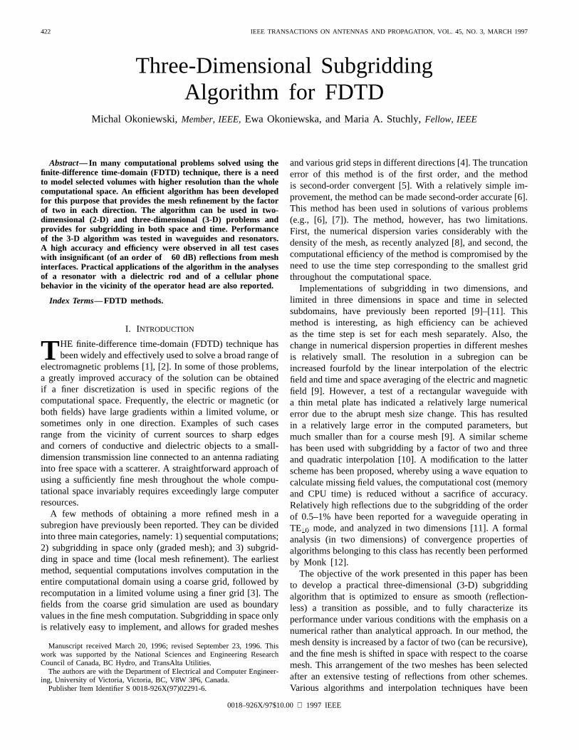
Fig. 1. The overlapping meshes adopted in the subgridding algorithm. Notethat coarse and fine meshes are offset inz direction. Gray region indicatesoverlapping pulsing mesh area.

evaluated. A pulsing, overlapping scheme of computations ofthe electric and magnetic fields in time and space for the twomeshes has been found to yield the best results. The greatestemphasis has been placed on a smooth transition between thecoarse and fine meshes. To achieve this, extrapolation in timeand interpolation in time and space are used, both accurateto the second order. The boundary of the two grids is usuallypositioned in a homogeneous region of the structure where thefield components and their derivatives have smooth behavior.Very low reflections (below 60 dB) can be obtained in a wide-frequency range, and the accuracy of computations can besignificantly increased without an excessive increase in thecomputational burden. The algorithm can also be used forheterogeneous interfaces with somewhat increased reflections.

II. SUBGRIDDING ALGORITHM

The following conditions guided the development of thealgorithm.

• The same stability condition should be used throughoutthe problem space.

• To minimize the reflections from the fine mesh, smallscaling factors and a sequence of subgrids, rather than anabrupt transition into much finer mesh, should be used.

As the first step of our development of a subgriddingalgorithm, we considered various mesh layouts and sub-gridding algorithms, including, for a two-dimensional (2-D)case, those previously reported in the literature. A number ofschemes produced good results in two dimesnions, but their3-D counterparts were of inferior quality and often sufferedfrom instability problems. We decided to base our algorithmon interpolation/extrapolation rather than on interpolation andwave equation, as in [9] and [10]. This approach was selected

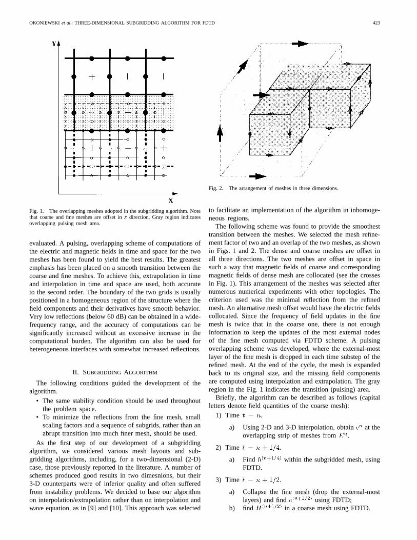
Fig. 2. The arrangement of meshes in three dimensions.

to facilitate an implementation of the algorithm in inhomoge-neous regions.

The following scheme was found to provide the smoothesttransition between the meshes. We selected the mesh refine-ment factor of two and an overlap of the two meshes, as shownin Figs. 1 and 2. The dense and coarse meshes are offset inall three directions. The two meshes are offset in space insuch a way that magnetic fields of coarse and correspondingmagnetic fields of dense mesh are collocated (see the crossesin Fig. 1). This arrangement of the meshes was selected afternumerous numerical experiments with other topologies. Thecriterion used was the minimal reflection from the refinedmesh. An alternative mesh offset would have the electric fieldscollocated. Since the frequency of field updates in the finemesh is twice that in the coarse one, there is not enoughinformation to keep the updates of the most external nodesof the fine mesh computed via FDTD scheme. A pulsingoverlapping scheme was developed, where the external-mostlayer of the fine mesh is dropped in each time substep of therefined mesh. At the end of the cycle, the mesh is expandedback to its original size, and the missing field componentsare computed using interpolation and extrapolation. The grayregion in the Fig. 1 indicates the transition (pulsing) area.

Briefly, the algorithm can be described as follows (capitalletters denote field quantities of the coarse mesh):

1) Time .

a) Using 2-D and 3-D interpolation, obtain at theoverlapping strip of meshes from .

2) Time .

a) Find within the subgridded mesh, usingFDTD.

3) Time .

a) Collapse the fine mesh (drop the external-mostlayers) and find using FDTD;

b) find in a coarse mesh using FDTD.


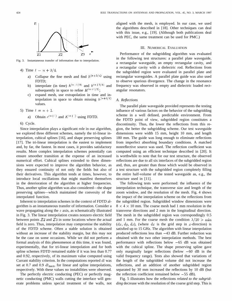
Fig. 3. Instantaneous transfer of information due to interpolation.

4) Time .

a) Collapse the fine mesh and find usingFDTD;

b) interpolate (in time) and andsubsequently in space to refine ;

c) expand mesh, use extrapolation in time and in-terpolation in space to obtain missingvalues.

5) Time .

a) Obtain and using FDTD.

6) Cycle.

Since interpolation plays a significant role in our algorithm,we explored three different schemes, namely the tri-linear in-terpolation, cubical splines [16], and shape preserving splines[17]. The tri-linear interpolation is the easiest to implementand, by far, the fastest. In most cases, it provides satisfactoryresults. More complex interpolation schemes potentially canensure smoother transition at the expense of an increasednumerical effort. Cubical splines extended to three dimen-sions were expected to improve the algorithm behavior, asthey ensured continuity of not only the fields but also oftheir derivatives. This algorithm tends at times, however, tointroduce local oscillations that might manifest themselvesin the deterioration of the algorithm at higher frequencies.Thus, another spline algorithm was also considered—the shapepreserving splines—which maintained the convexity of theinterpolated function.

Inherent to interpolation schemes in the context of FDTD al-gorithm is an instantaneous transfer of information. Consider awave propagating along theaxis, as schematically illustratedin Fig. 3. The linear interpolation creates nonzero electric fieldbetween points and in some locations where the actualfield is zero. Thus, interpolation may compromise the stabilityof the FDTD scheme. Often a stable solution is obtainedwithout an increase of the stability margin, but this may notbe the case on some occasions. While we did not perform aformal analysis of this phenomenon at this time, it was found,experimentally, that for tri-linear interpolation and for bothspline schemes FDTD remained stable if it was less than 0.77and 0.92, respectively, of its maximum value computed usingCurrant stability criterion. In the computations reportedwasset at 0.7 and 0.9 , for linear and spline interpolations,respectively. With these values no instabilities were observed.

The perfectly electric conducting (PEC) or perfectly mag-netic conducting (PMC) walls cutting the interface will gen-erate problems unless special treatment of the walls, not

aligned with the mesh, is employed. In our case, we usedthe algorithms described in [18]. Other techniques can dealwith this issue, e.g., [19]. (Although both publications dealwith PEC, the same treatment can be used for PMC.)

III. N UMERICAL EVALUATION

Performance of the subgridding algorithm was evaluatedin the following test structures: a parallel plate waveguide,a rectangular waveguide, an empty rectangular cavity, anda rectangular cavity with a dielectric rod. Reflections fromthe subgridded region were evaluated in parallel plate andrectangular waveguides. A parallel plate guide was also usedto observe spurious divergence. The change in the resonancefrequency was observed in empty and dielectric loaded rect-angular resonators.

A. Reflections

The parallel plate waveguide provided represents the testinginfluence of various factors on the behavior of the subgriddingscheme in a well defined, predictable environment. Fromthe FDTD point of view, subgridded region constitutes adiscontinuity. Thus, the lower the reflections from this re-gion, the better the subgridding scheme. Our test waveguidedimensions were width 15 mm, height 10 mm, and length180 mm. The guide was long enough to eliminate reflectionsfrom imperfect absorbing boundary conditions. A matchednonreflective source was used. The reflection coefficient wascomputed using an efficient technique described in [20]. Itis worthwhile to note that for our test structure, the observedreflections are due to all six interfaces of the subgridded regionand, thus, are greater than those which would be observed ina test structure with the subgridded region completely fillingthe entire half-volume of the tested waveguide as, e.g., thestructure used in [11].

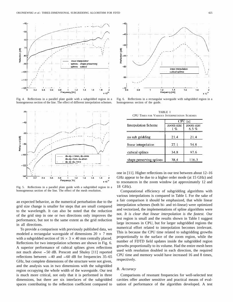
The following tests were performed: the influence of theinterpolation technique, the transverse size and length of thezoom window, and the resolution of the mesh. Fig. 4 showsthe impact of the interpolation scheme on the reflections fromthe subgridded region. Subgridded window dimensions were8 4 10 mm. The coarse mesh had 1 mm resolution in thetransverse directions and 2 mm in the longitudinal direction.The mesh in the subgridded region was correspondingly 0.5and 1 mm. For the coarse mesh the condition( ), (where is the grid step in -direction) issatisfied up to 15 GHz. The algorithm with linear interpolationproduced reflections less than43 dB. Further reduction wasobtained with the two other interpolation methods. The bestperformance with reflections below 65 dB was obtainedwith the cubical spline. The shape preserving spline gaveonly marginally larger reflections (below 60 dB in thevalid frequency range). Tests also showed that variations ofthe length of the subgridded volume did not increase thereflections, and an addition of another subgridded regionseparated by 30 mm increased the reflections by 10 dB (butthe reflection coefficient remained below55 dB).

Fig. 5 illustrates how the reflectionsrelated to the subgrid-dingdecrease with the resolution of the coarse grid step. This is


Fig. 4. Reflections in a parallel plate guide with a subgridded region in ahomogeneous section of the line. The effect of different interpolation schemes.

Fig. 5. Reflections in a parallel plate guide with a subgridded region in ahomogeneous section of the line. The effect of the mesh resolution.

an expected behavior, as the numerical perturbation due to thegrid size change is smaller for steps that are small comparedto the wavelength. It can also be noted that the reductionof the grid step in one or two directions only improves theperformance, but not to the same extent as the grid reductionin all directions.

To provide a comparison with previously published data, wemodeled a rectangular waveguide of dimensions 207 mmwith a subgridded section of 16 3 40 mm centrally placed.Reflections for two interpolation schemes are shown in Fig. 6.A superior performance of cubical splines gives reflectionsnot much above 50 dB. Prescott and Shuley [11] reportedreflections between 40 and 60 dB for frequencies 35–65GHz, but complete dimensions of the structure were not given,and the analysis was in two dimensions with the subgriddedregion occupying the whole width of the waveguide. Our testis much more critical, not only that it is performed in threedimensions, but there are six interfaces of the subgriddedspaces contributing to the reflection coefficient compared to

Fig. 6. Reflections in a rectangular waveguide with subgridded region in ahomogeneous section of the guide.

TABLE ICPU TIMES FOR VARIOUS INTERPRETATION SCHEMES

one in [11]. Higher reflections in our test between about 12–16GHz appear to be due to a higher order mode (at 15 GHz) andto resonances in the zoom window (at approximately 12 and18 GHz).

Computational efficiency of subgridding algorithms withvarious interpolations is compared in Table I. For the sake ofa fair comparison it should be emphasized, that while linearinterpolation schemes (both bi- and tri-linear) were optimizedand vectorized, the implementations of spline algorithms werenot. It is clear that linear interpolation is the fastest.Ourtest region is small and the results shown in Table I suggestlarge increases in CPU, but for larger subgridded regions thenumerical effort related to interpolation becomes irrelevant.This is because the CPU time related to subgridding growthsproportionally to the surface of the zoom region, while thenumber of FDTD field updates inside the subgridded regiongrowths proportionally to its volume. Had the entire mesh beenused with resolution doubled in each direction, the requiredCPU time and memory would have increased 16 and 8 times,respectively.

B. Accuracy

Comparisons of resonant frequencies for well-selected testcavities offer another sensitive and practical means of eval-uation of performance of the algorithm developed. A test


(a) (b) (c)

(d) (e) (f)

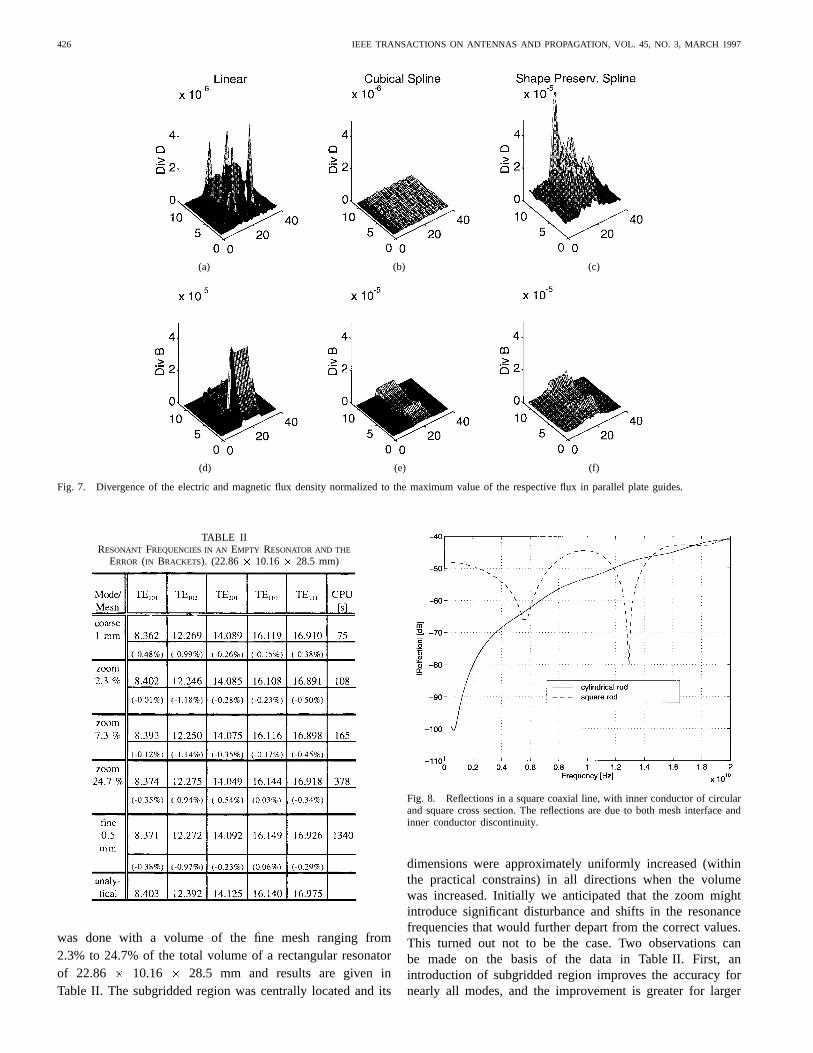
Fig. 7. Divergence of the electric and magnetic flux density normalized to the maximum value of the respective flux in parallel plate guides.

TABLE IIRESONANT FREQUENCIES IN AN EMPTY RESONATOR AND THE

ERROR (IN BRACKETS). (22.86� 10.16� 28.5 mm)

was done with a volume of the fine mesh ranging from2.3% to 24.7% of the total volume of a rectangular resonatorof 22.86 10.16 28.5 mm and results are given inTable II. The subgridded region was centrally located and its

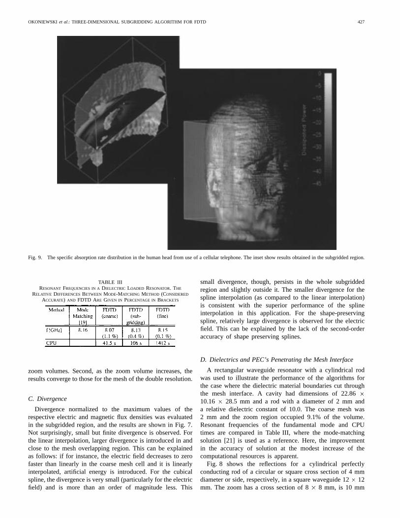
Fig. 8. Reflections in a square coaxial line, with inner conductor of circularand square cross section. The reflections are due to both mesh interface andinner conductor discontinuity.

dimensions were approximately uniformly increased (withinthe practical constrains) in all directions when the volumewas increased. Initially we anticipated that the zoom mightintroduce significant disturbance and shifts in the resonancefrequencies that would further depart from the correct values.This turned out not to be the case. Two observations canbe made on the basis of the data in Table II. First, anintroduction of subgridded region improves the accuracy fornearly all modes, and the improvement is greater for larger


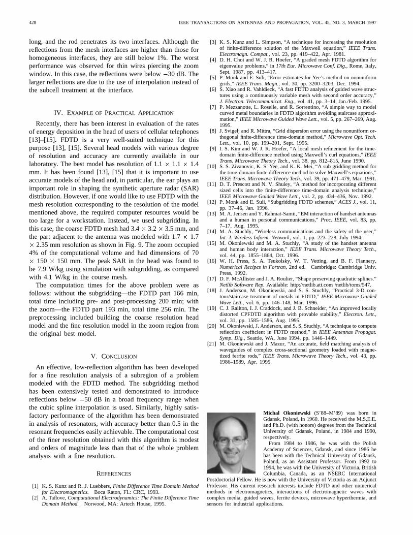
Fig. 9. The specific absorption rate distribution in the human head from use of a cellular telephone. The inset show results obtained in the subgridded region.

TABLE IIIRESONANT FREQUENCIES IN A DIELECTRIC LOADED RESONATOR. THE

RELATIVE DIFFERENCESBETWEEN MODE-MATCHING METHOD (CONSIDERED

ACCURATE) AND FDTD ARE GIVEN IN PERCENTAGE IN BRACKETS

zoom volumes. Second, as the zoom volume increases, theresults converge to those for the mesh of the double resolution.

C. Divergence

Divergence normalized to the maximum values of therespective electric and magnetic flux densities was evaluatedin the subgridded region, and the results are shown in Fig. 7.Not surprisingly, small but finite divergence is observed. Forthe linear interpolation, larger divergence is introduced in andclose to the mesh overlapping region. This can be explainedas follows: if for instance, the electric field decreases to zerofaster than linearly in the coarse mesh cell and it is linearlyinterpolated, artificial energy is introduced. For the cubicalspline, the divergence is very small (particularly for the electricfield) and is more than an order of magnitude less. This

small divergence, though, persists in the whole subgriddedregion and slightly outside it. The smaller divergence for thespline interpolation (as compared to the linear interpolation)is consistent with the superior performance of the splineinterpolation in this application. For the shape-preservingspline, relatively large divergence is observed for the electricfield. This can be explained by the lack of the second-orderaccuracy of shape preserving splines.

D. Dielectrics and PEC’s Penetrating the Mesh Interface

A rectangular waveguide resonator with a cylindrical rodwas used to illustrate the performance of the algorithms forthe case where the dielectric material boundaries cut throughthe mesh interface. A cavity had dimensions of 22.8610.16 28.5 mm and a rod with a diameter of 2 mm anda relative dielectric constant of 10.0. The coarse mesh was2 mm and the zoom region occupied 9.1% of the volume.Resonant frequencies of the fundamental mode and CPUtimes are compared in Table III, where the mode-matchingsolution [21] is used as a reference. Here, the improvementin the accuracy of solution at the modest increase of thecomputational resources is apparent.

Fig. 8 shows the reflections for a cylindrical perfectlyconducting rod of a circular or square cross section of 4 mmdiameter or side, respectively, in a square waveguide 1212mm. The zoom has a cross section of 88 mm, is 10 mm


long, and the rod penetrates its two interfaces. Although thereflections from the mesh interfaces are higher than those forhomogeneous interfaces, they are still below 1%. The worstperformance was observed for thin wires piercing the zoomwindow. In this case, the reflections were below30 dB. Thelarger reflections are due to the use of interpolation instead ofthe subcell treatment at the interface.

IV. EXAMPLE OF PRACTICAL APPLICATION

Recently, there has been interest in evaluation of the ratesof energy deposition in the head of users of cellular telephones[13]–[15]. FDTD is a very well-suited technique for thispurpose [13], [15]. Several head models with various degreeof resolution and accuracy are currently available in ourlaboratory. The best model has resolution of 1.11.1 1.4mm. It has been found [13], [15] that it is important to useaccurate models of the head and, in particular, the ear plays animportant role in shaping the synthetic aperture radar (SAR)distribution. However, if one would like to use FDTD with themesh resolution corresponding to the resolution of the modelmentioned above, the required computer resources would betoo large for a workstation. Instead, we used subgridding. Inthis case, the coarse FDTD mesh had 3.43.2 3.5 mm, andthe part adjacent to the antenna was modeled with 1.71.7

2.35 mm resolution as shown in Fig. 9. The zoom occupied4% of the computational volume and had dimensions of 70

150 150 mm. The peak SAR in the head was found tobe 7.9 W/kg using simulation with subgridding, as comparedwith 4.1 W/kg in the course mesh.

The computation times for the above problem were asfollows: without the subgridding—the FDTD part 166 min,total time including pre- and post-processing 200 min; withthe zoom—the FDTD part 193 min, total time 256 min. Thepreprocessing included building the coarse resolution headmodel and the fine resolution model in the zoom region fromthe original best model.

V. CONCLUSION

An effective, low-reflection algorithm has been developedfor a fine resolution analysis of a subregion of a problemmodeled with the FDTD method. The subgridding methodhas been extensively tested and demonstrated to introducereflections below 50 dB in a broad frequency range whenthe cubic spline interpolation is used. Similarly, highly satis-factory performance of the algorithm has been demonstratedin analysis of resonators, with accuracy better than 0.5 in theresonant frequencies easily achievable. The computational costof the finer resolution obtained with this algorithm is modestand orders of magnitude less than that of the whole problemanalysis with a fine resolution.

REFERENCES

[1] K. S. Kunz and R. J. Luebbers,Finite Difference Time Domain Methodfor Electromagnetics. Boca Raton, FL: CRC, 1993.

[2] A. Taflove,Computational Electrodynamics: The Finite Difference TimeDomain Method. Norwood, MA: Artech House, 1995.

[3] K. S. Kunz and L. Simpson, “A technique for increasing the resolutionof finite-difference solution of the Maxwell equation,”IEEE Trans.Electromagn. Compat.,vol. 23, pp. 419–422, Apr. 1981.

[4] D. H. Choi and W. J. R. Hoefer, “A graded mesh FDTD algorithm foreigenvalue problems,” in17th Eur. Microwave Conf. Dig., Rome, Italy,Sept. 1987, pp. 413–417.

[5] P. Monk and E. Suli, “Error estimates for Yee’s method on nonuniformgrids,” IEEE Trans. Magn.,vol. 30, pp. 3200–3203, Dec. 1994.

[6] S. Xiao and R. Vahldieck, “A fast FDTD analysis of guided wave struc-tures using a continuously variable mesh with second order accuracy,”J. Electron. Telecommunicat. Eng.,vol. 41, pp. 3–14, Jan./Feb. 1995.

[7] P. Mezzanotte, L. Roselle, and R. Sorrentino, “A simple way to modelcurved metal boundaries in FDTD algorithm avoiding staircase approxi-mation,” IEEE Microwave Guided Wave Lett., vol. 5, pp. 267–269, Aug.1995.

[8] J. Svigelj and R. Mittra, “Grid dispersion error using the nonuniform or-thogonal finite-difference time-domain method,”Microwave Opt. Tech.Lett., vol. 10, pp. 199–201, Sept. 1995.

[9] I. S. Kim and W. J. R. Hoefer, “A local mesh refinement for the time-domain finite-difference method using Maxwell’s curl equations,”IEEETrans. Microwave Theory Tech.,vol. 38, pp. 812–815, June 1990.

[10] S. S. Zivanovic, K. S. Yee, and K. K. Mei, “A sub gridding method forthe time-domain finite difference method to solve Maxwell’s equations,”IEEE Trans. Microwave Theory Tech.,vol. 39, pp. 471–479, Mar. 1991.

[11] D. T. Prescott and N. V. Shuley, “A method for incorporating differentsized cells into the finite-difference time-domain analysis technique,”IEEE Microwave Guided Wave Lett., vol. 2, pp. 434–436, Nov. 1992.

[12] P. Monk and E. Suli, “Subgridding FDTD schemes,”ACES J.,vol. 11,pp. 37–46, Jan. 1996.

[13] M. A. Jensen and Y. Rahmat-Samii, “EM interaction of handset antennasand a human in personal communications,”Proc. IEEE, vol. 83, pp.7–17, Aug. 1995.

[14] M. A. Stuchly, “Wireless communications and the safety of the user,”Int. J. Wireless Inform. Network, vol. 1, pp. 223–228, July 1994.

[15] M. Okoniewski and M. A. Stuchly, “A study of the handset antennaand human body interaction,”IEEE Trans. Microwave Theory Tech.,vol. 44, pp. 1855–1864, Oct. 1996.

[16] W. H. Press, S. A. Teukolsky, W. T. Vetting, and B. F. Flannery,Numerical Recipes in Fortran, 2nd ed. Cambridge: Cambridge Univ.Press, 1992.

[17] D. F. McAllister and J. A. Roulier, “Shape preserving quadratic splines.”Netlib Software Rep.Available: http://netlib.att.com /netlib/toms/547.

[18] J. Anderson, M. Okoniewski, and S. S. Stuchly, “Practical 3-D con-tour/staircase treatment of metals in FDTD,”IEEE Microwave GuidedWave Lett., vol. 6, pp. 146–148, Mar. 1996.

[19] C. J. Railton, I. J. Craddock, and J. B. Schneider, “An improved locallydistorted CPFDTD algorithm with provable stability,”Electron. Lett.,vol. 31, pp. 1585–1586, Aug. 1995.

[20] M. Okoniewski, J. Anderson, and S. S. Stuchly, “A technique to computereflection coefficient in FDTD method,” inIEEE Antennas Propagat.Symp. Dig.,Seattle, WA, June 1994, pp. 1446–1449.

[21] M. Okoniewski and J. Mazur, “An accurate, field matching analysis ofwaveguides of complex cross-sectional geometry loaded with magne-tized ferrite rods,”IEEE Trans. Microwave Theory Tech.,vol. 43, pp.1986–1989, Apr. 1995.

Michal Okoniewski (S’88–M’89) was born inGdansk, Poland, in 1960. He received the M.S.E.E.and Ph.D. (with honors) degrees from the TechnicalUniversity of Gdansk, Poland, in 1984 and 1990,respectively.

From 1984 to 1986, he was with the PolishAcademy of Sciences, Gdansk, and since 1986 hehas been with the Technical University of Gdansk,Poland, as an Assistant Professor. From 1992 to1994, he was with the University of Victoria, BritishColumbia, Canada, as an NSERC International

Postdoctorial Fellow. He is now with the University of Victoria as an AdjunctProfessor. His current research interests include FDTD and other numericalmethods in electromagnetics, interactions of electromagnetic waves withcomplex media, guided waves, ferrite devices, microwave hyperthermia, andsensors for industrial applications.


Ewa Okoniewska received the M.S.E.E. degreefrom Technical University of Gdansk, Poland, in1984.

From 1986 to 1992, she was with the Techni-cal University of Gdansk, Poland. In 1993, shejoined the University of Victoria, British Columbia,Canada. Her research interests include microwavehyperthermia and bio-electromagnetics.

Maria A. Stuchly, (M’71–SM’76–F’91) receivedthe M.Sc. degree in electrical engineering fromWarsaw Technical University, Poland, in 1962, andthe Ph.D. degree in electrical engineering from thePolish Academy of Sciences, Warsaw, in 1970.

Between the years of 1962 and 1970, she waswith the Warsaw Technical University, Poland, andthe Institute of the Polish Academy of Sciences.After immigrating to Canada during 1970, her firstposition was with the University of Manitoba. In1976 she became employed by the Bureau of Ra-

diation and Medical Devices in Health and Welfare, Ottawa, Canada as aResearch Scientist. During 1978 she became associated with the ElectricalEngineering Department at the University of Ottawa, Canada, as an AdjunctProfessor, and from 1990 to 1991 she was a Funding Director of the Institute ofMedical Engineering, at the same university. In 1992 she joined the Universityof Victoria as a Visiting Professor with the Department of Electrical andComputer Engineering, and since January 1994, she has been a Professorand Industrial Research Chairholder, funded by the Natural Sciences andEngineering Research Council of Canada, BC Hydro, and Trans Alta Utilities.

Dr. Stuchly was President of the Bioelectromagnetic Society, the Chairmanof the International URSI Commission K “Electromagnetics in Biology andMedicine” (1991 to 1993), and was elected Vice-President of InternationalURSI in 1996.

Documents

Three-dimensional subgridding algorithm for FDTD