Embed Size (px)
Citation preview
Theoretical Computer Science 485 (2013) 69–84
Contents lists available at SciVerse ScienceDirect
Theoretical Computer Science
journal homepage: www.elsevier.com/locate/tcs
Tight complexity bounds for FPT subgraph problemsparameterized by the clique-width✩
Hajo Broersma a, Petr A. Golovach b,∗, Viresh Patel ca Faculty of EEMCS, University of Twente, P.O. Box 217, 7500 AE Enschede, The Netherlandsb Department of Informatics, University of Bergen, P.O. Box 7803, 5020 Bergen, Norwayc School of Mathematics, Birmingham University, Edgbaston, Birmingham, B15 2TT, UK
a r t i c l e i n f o
Article history:Received 11 July 2012Received in revised form 26 February 2013Accepted 4 March 2013Communicated by V.Th. Paschos
Keywords:Parameterized complexityClique-widthExponential Time Hypothesis
a b s t r a c t
We give tight algorithmic lower and upper bounds for some double-parameterizedsubgraph problems when the clique-width of the input graph is one of the parameters.Let G be an arbitrary input graph on n vertices with clique-width at most w. We prove thefollowing results.
• The Dense (Sparse) k-Subgraph problem, which asks whether there exists an inducedsubgraph of G with k vertices and at least q edges (at most q edges, respectively), canbe solved in time kO(w)
· n, but it cannot be solved in time 2o(w log k)· nO(1) unless the
Exponential Time Hypothesis (ETH) fails.• The d-Regular Induced Subgraph problem, which asks whether there exists a
d-regular induced subgraph of G, and the Minimum Subgraph of Minimum Degree atleast d problem, which asks whether there exists a subgraph of G with k vertices andminimum degree at least d, can be solved in time dO(w)
· n, but they cannot be solved intime 2o(w log d)
· nO(1) unless ETH fails.
© 2013 Elsevier B.V. All rights reserved.
1. Introduction
The notion of clique-width introduced by Courcelle and Olariu [13] (we refer the reader to the survey [23] for furtherinformation on differentwidth parameters) has nowbecome one of the fundamental parameters in Graph Algorithms.Manyproblemswhich are hard on general graphs can be solved efficientlywhen the input is restricted to graphs of bounded clique-width. Themeta-theorem of Courcelle, Makowsky, and Rotics [12] states that all problems expressible inMS1-logic are fixedparameter tractable (FPT), when parameterized by the clique-width of the input graph (see the books of Downey and Fellows[17] and Flum and Grohe [20] for a detailed treatment of parameterized complexity). In other words, this theorem showsthat any problem expressible in MS1-logic can be solved for graphs of clique-width at most w in time f (w) · |I|O(1), where|I| is the size of the input and f is a computable function depending on the parameter w only. Here, the superexponentialfunction f is defined by a logic formula, and it grows very fast.
The basic method for constructing algorithms for graphs of bounded clique-width is to use dynamic programming alongan expression tree (the definition is given in Section 2). Computing clique-width is an NP-hard problem [19], but it can beapproximated and a corresponding expression tree can be constructed in FPT-time [22,31]. In our paper it is always assumed
✩ Preliminary extended abstract of this paper appeared in the proceedings of IPEC 2011.∗ Corresponding author. Tel.: +47 55584385.
E-mail addresses: [email protected] (H. Broersma), [email protected] (P.A. Golovach), [email protected] (V. Patel).
0304-3975/$ – see front matter© 2013 Elsevier B.V. All rights reserved.http://dx.doi.org/10.1016/j.tcs.2013.03.008
70 H. Broersma et al. / Theoretical Computer Science 485 (2013) 69–84
that an expression tree is given. In this case dynamic programming algorithms can be relatively efficient: usually single-exponential in the clique-width. A natural question to ask iswhether the running times of such algorithms are asymptoticallyoptimal up to some reasonable complexity conjectures.
The Exponential Time Hypothesis (ETH) [24] asserts that there does not exist an algorithm for solving 3-SAT runningin time 2o(n) on a formula with n variables; this is equivalent to the parameterized complexity conjecture that FPT =
M[1] [16,20]. The Exponential Time Hypothesis has proved to be an effective tool for establishing tight complexity boundsfor parameterized problems. We refer the reader to the survey by Lokshtanov, Marx and Saurabh [27] for an overview ofthe field and mention here only some results related to our paper. Chen et al. [7–9] showed that there is no algorithm fork-Clique running in time f (k)no(k), for n-vertex graphs, unless ETH fails (on the other hand it is easily seen that k-Clique canbe solved in time nO(k)). The lower bound on the k-Clique problem can be extended to some other parameterized problemsvia linear FPT-reductions [8,9]. In particular, for problems parameterized by clique-width, Fomin et al. [21] proved thatMax-Cut and Edge Dominating Set cannot be solved in time f (w)no(w) on n-vertex graphs of clique-width at mostw, unless ETHcollapses. Lokshtanov, Marx and Saurabh [28] considered several FPT problems solvable in time 2O(k log k)
· |I|O(1) and showedthat a 2o(k log k)
· |I|O(1)-time algorithm for these problems would violate ETH. To do this, they introduced special restrictedversions of some basic problems like k-Clique on graphs with k2 vertices (and with some other restrictions) and provedthat these problems cannot be solved in time 2o(k log k)
· kO(1) unless ETH collapses. These results open the possibility ofestablishing algorithmic lower bounds for natural problems. We use this approach to prove asymptotically tight bounds forsome double-parameterized subgraph problems when the clique-width of the input graph is one of the parameters. Theseresults give the first known bounds for such types of problems parameterized by clique-width.
First, we consider the Dense k-Subgraph problem (also known as the k-Cluster problem). This problem asks whether,given a graph G and positive integers k and q, there exists an induced subgraph of G with k vertices and at least q edges.Clearly, Dense k-Subgraph is NP-hard since it is a generalization of the k-Clique problem. It remains NP-hard, even whenrestricted to comparability graphs, bipartite graphs and chordal graphs [11], as well as on planar graphs [25]. Polynomialalgorithms were given for cographs, split graphs [11], and for graphs of bounded tree-width [25]. Considerable work hasbeen done on approximation algorithms for this problem [3,4,14,18,26].
Next, we consider some degree-constrained subgraph problems. The objective in such problems is to find a subgraphsatisfying certain lower or upper bounds on the degree of each vertex. Typically it is necessary to either check the existenceof a subgraph satisfying the degree constraints or tominimize (maximize) someparameter (usually the size of the subgraph).
The d-Regular Subgraph problem,which askswhether a given graph contains a d-regular subgraph, has been intensivelystudied. We mention here only some complexity results. Chvátal et al. [10] proved that this problem is NP-complete ford = 3. It was shown that the problem with d = 3 remains NP-complete for planar bipartite graphs with maximum degreefour, and that when d ≥ 3, it is NP-complete even for bipartite graphs with maximum degree at most d + 1. Some furtherresults were given in [6,32–34]. We consider a variant of this problem called d-Regular Induced Subgraph, where weask whether a given graph G contains a d-regular induced subgraph. This variant of the problem has also been studied. Inparticular, the parameterized complexity of different variants of the problemwas considered byMoser and Thilikos [30] andby Mathieson and Szeider [29]. Observe that, trivially, d-Regular Induced Subgraph can be solved in polynomial time ford ≤ 2, and it easily follows from the known hardness results for d-Regular Subgraph that d-Regular Induced Subgraph isNP-complete for any fixed d ≥ 3.
In [2] Amini et al. introduced the Minimum Subgraph of Minimum Degree at least d problem. This problem askswhether, given a graph G and positive integers d and k, there exists a subgraph of Gwith atmost k vertices andminimumde-gree at least d. The parameterized complexity of the problemwas considered in [2]. Some other hardness and approximationresults can be found in [1].
Our main results and the organization of the paper. In Section 2 we give some basic definitions and some preliminary results.In Section 3 we consider the Dense k-Subgraph and Sparse k-Subgraph problems. The Sparse k-Subgraph problem is dualto Dense k-Subgraph and it asks whether, given a graph G and positive integers k and q, there exists an induced subgraphof G with k vertices and at most q edges. We prove that these problems can be solved in time kO(w)
· n for n-vertex graphsof clique-width at most w if an expression tree of width w is given, but they cannot be solved in time 2o(w log k)
· nO(1) unlessETH fails even if an expression tree of width w is included in the input. In Sections 4 and 5 we consider the d-RegularInduced Subgraph and Minimum Subgraph of Minimum Degree at least d problems respectively. We construct dynamicprogramming algorithms which solve these problems in time dO(w)
· n for n-vertex graphs of clique-width at most w if anexpression tree of width w is given, and then prove that these problems cannot be solved in time 2o(w log d)
· nO(1) unless ETHfails even if an expression tree of width w is provided. We conclude the paper with some open problems.
2. Definitions and preliminary results
Graphs. We consider finite undirected graphs without loops or multiple edges. The vertex set of a graph G is denoted byV (G) and its edge set by E(G). A set S ⊆ V (G) of pairwise adjacent vertices is called a clique. For v ∈ V (G), EG(v) denotes theset of edges incident with v. The degree of a vertex v is denoted by dG(v). For a non-negative integer d, a graph G is calledd-regular if all vertices of G have degree d. For a graph G, the incidence graph of G is the bipartite graph I(G) with vertex
H. Broersma et al. / Theoretical Computer Science 485 (2013) 69–84 71
set V (G) ∪ E(G) such that v ∈ V (G) and e ∈ E(G) are adjacent if and only if v is incident with e in G. We denote by G thecomplement of a graph G, i.e. the graph with vertex set V (G) such that any two distinct vertices are adjacent in G if and onlyif they are non-adjacent in G. For a set of vertices S ⊆ V (G), G[S] denotes the subgraph of G induced by S, and by G − S wedenote the graph obtained from G by the removal of all the vertices of S, i.e. the subgraph of G induced by V (G) \ S.
Clique-width. Let G be a graph, and let w be a positive integer. A w-graph is a graph whose vertices are labeled by integersfrom {1, 2, . . . , w}. We call the w-graph consisting of exactly one vertex v labeled by some integer i from {1, 2, . . . , w}
an initial w-graph. The clique-width cwd(G) is the smallest integer w such that G can be constructed by means of repeatedapplication of the following four operations: (1) introduce: construction of an initial w-graph with vertex v labeled by i(denoted by i(v)), (2) disjoint union (denoted by ⊕), (3) relabel: changing the labels of each vertex labeled i to j (denoted byρi→j) and (4) join: joining all vertices labeled by i to all vertices labeled by j by edges (denoted by ηi,j).
An expression tree of a graph G is a rooted tree T of the following form.
• The nodes of T are of four types: i, ⊕, η and ρ.• Introduce nodes i(v) are leaves of T , and they correspond to initial w-graphs with vertices v, which are labeled i.• A union node ⊕ stands for a disjoint union of graphs associated with its children.• A relabel node ρi→j has one child and is associated with thew-graph resulting from the relabeling operation ρi→j applied
to the graph corresponding to the child.• A join node ηi,j has one child and is associatedwith thew-graph resulting from the join operation ηi,j applied to the graph
corresponding to the child.• The graph G is isomorphic to the graph associated with the root of T (with all labels removed).
The width of the tree T is the number of different labels appearing in T . If a graph G has cwd(G) ≤ w then it is possibleto construct a rooted expression tree T of G with width w. Given a node X of an expression tree, the graph GX is the graphformed by the subtree of the expression tree rooted at X .
Parameterized reductions. We refer the reader to the books [17,20] for a detailed treatment of parameterized complexity.Here we only define the notion of parameterized (linear) reduction, which is the main tool for establishing our results. Forparameterized problems A, B, we say that A is (uniformly many:1) FPT-reducible to B if there exist functions f , g : N → N, aconstant α ∈ N and an algorithm Φ which transforms an instance (x, k) of A into an instance (x′, g(k)) of B in time f (k)|x|αso that (x, k) ∈ A if and only if (x′, g(k)) ∈ B. The reduction is called linear if g(k) = O(k).
Capacitated domination. For our reductions we use a variant of the Capacitated Dominating Set problem. Theparameterized complexity of this problem, with the tree-width of the input graph being the parameter, was consideredin [5,15].
A red–blue capacitated graph is a pair (G, c), where G is a bipartite graph with a vertex bipartition into sets R and B, andc : R → N is a capacity function such that 1 ≤ c(v) ≤ dG(v) for every vertex v ∈ R. The vertices of the set R are called red andthe vertices of B are called blue. A set S ⊆ R is called a capacitated dominating set if there is a domination mapping f : B → Swhich maps every vertex in B to one of its neighbors such that the total number of vertices mapped by f to any vertex v ∈ Sdoes not exceed its capacity c(v). We say that for a vertex v ∈ S, vertices in the set f −1(v) are dominated by v. The Red–BlueCapacitated Dominating Set (or Red–Blue CDS) problem asks whether, given a red–blue capacitated graph (G, c) and apositive integer k, there exists a capacitated dominating set S for G containing at most k vertices. A capacitated dominatingset S ⊆ R is called saturated if there is a domination mapping f which saturates all vertices of S, that is, |f −1(v)| = c(v)for each v ∈ S. The Red–Blue Exact Saturated Dominating Set problem (Red–Blue Exact Saturated CDS) takes a red–blue capacitated graph (G, c) and a positive integer k as an input and asks whether there exists a saturated capacitateddominating set with exactly k vertices.
The next proposition immediately follows from the results proved in [21].
Proposition 1. The Red–Blue CDS and Red–Blue Exact Saturated CDS problems cannot be solved in time f (w) · no(w), wheren is the number of vertices of the input graph G and w is the clique-width of the incidence graph I(G), unless ETH fails, even if anexpression tree of width w for I(G) is given.
The proof of Proposition 1 uses the result of Chen et al. [7–9] that there is no algorithm for k-Clique (finding a cliqueof size k) running in time f (k) · no(k) unless there exists an algorithm for solving 3-SAT running in time 2o(n) on a formulawith n variables. Proposition 1 was proved via a linear reduction from the k-Multi-Colored Clique problem (see [5,21]).The k-Multi-Colored Clique problem asks for a given k-partite graph G = (V1 ∪ · · · ∪ Vk, E), where V1, . . . , Vk are sets ofthe k-partition, whether there is a k-clique in G. It should be noted that the construction of an expression tree of boundedwidth is part of the reduction and it is done in polynomial time. Lokshtanov, Marx and Saurabh [28] considered a specialrestricted variant of k-Multi-Colored Clique called k×k-Clique. In this variant of the problem |V1| = · · · = |Vk| = k. Theyproved the following.
Proposition 2 ([28]). The k × k-Clique problem cannot be solved in time 2o(k log k)· nO(1), where n is the number of vertices of
the input graph G, unless ETH fails.
72 H. Broersma et al. / Theoretical Computer Science 485 (2013) 69–84
By replacing k-Multi-Colored Clique by the k× k-Clique problem in the reductions used for the proof of Proposition 1,we obtain the following corollary.
Corollary 1. The Red–Blue CDS and Red–Blue Exact Saturated CDS problems cannot be solved in time 2o(w log n)·nO(1), where
n is the number of vertices of the input graph G and w is the clique-width of the incidence graph I(G), unless ETH fails, even if anexpression tree of width w for I(G) is given.
Observe that Corollary 1 gives a slightly stronger claim than Proposition 1: while o(w) · log n = o(w log n), it is not sothe other way around.
3. Sparse and Dense k-Subgraph problems
In this section we consider the Dense k-Subgraph and Sparse k-Subgraph problems. The aim of this section is the proofof the following theorem.
Theorem 1. The Sparse k-Subgraph problem can be solved in time kO(w)· n on n-vertex graphs of clique-width at most w if an
expression tree of width w is given, but it cannot be solved in time 2o(w log k)· nO(1) unless ETH fails, even if an expression tree of
width w is given.
Clearly, Sparse k-Subgraph and Dense k-Subgraph are dual, i.e. Sparse k-Subgraph is equivalent to Dense k-Subgraphfor the complement of the input graph. Since for any graph G, cwd(G) ≤ 2 · cwd(G) (see e.g. [13,35]), we can immediatelyget the following corollary.
Corollary 2. The Dense k-Subgraph problem can be solved in time kO(w)· n on n-vertex graphs of clique-width at most w if an
expression tree of width w is given, but it cannot be solved in time 2o(w log k)· nO(1) unless ETH fails, even if an expression tree of
width w is given.
3.1. Algorithmic upper bounds for Sparse k-Subgraph
We sketch a dynamic programming algorithm for solving Sparse k-Subgraph in time kO(w)· n on graphs of clique-width
at most w. The algorithm is based on the following observation.Let G be a graph with n vertices, and let T be an expression tree for G of width w. For a node X of T , let U1(X), . . . ,Uw(X)
be the sets of vertices of GX labeled 1, . . . , w, respectively. Recall that for a graph G, we are looking for an induced subgraphH on k vertices with at most q edges. For a node X of T , denote by HX the subgraph of GX induced by V (H) ∩ V (GX ) (it canhappen that V (H) ∩ V (GX ) = ∅). If X is an introduce node, then HX has no edges. If X is a relabel node, then the numberof edges of HX is the same as the number of edges of HY for the unique child Y of X . If X is a union node, then the numberof edges of HX is the sum of the numbers of edges of HY and HZ where Y and Z are the children of X . Finally, if X is a joinnode ηi,j, then |E(HX )| = |EY | + sisj where Y is the unique child of X and si, sj are the number of vertices of HX labeled i andj respectively in GX . It indicates that each partial solution for a node X can be encoded as the minimum number of edges ofan induced subgraph of GX that has exactly si vertices of Ui(X) for i ∈ {1, . . . , w}.
Nowwe describe formally what we store in the tables corresponding to the nodes in an expression tree. The table of datafor the node X contains entries which store a positive integer p ≤ q and a vector (s1, . . . , sw) of non-negative integers suchthat s = s1 + · · · + sw ≤ k for i ∈ {1, . . . , w}, for which p is the minimum number of edges of an induced subgraph H withs vertices such that for i ∈ {1, . . . , w}, si = |Ui(X) ∩ V (H)|. If X is the root node of T then G contains an induced subgraphwith k vertices and at most q edges if and only if the table for X contains an entry with the parameter p ≤ q and vector(s1, . . . , sw) such that s1 + · · · + sw = k.
We create and update the tables as follows.
Introduce Node: Tables for introduce nodes of T are constructed in a straightforward manner. Suppose that X = i(v) forv ∈ V (G) and i ∈ {1, . . . , w}. Then the table of data for the node X contains two entries with p = 0 and the vectors(s1, . . . , sw) such that sj = 0 for j ∈ {1, . . . , w}, j = i, si = 0 for the first entry and si = 1 for the second.
Relabel Node: Suppose that X is a relabel node ρi→j, and Y is a child of X . Then the table for X contains an entry with aninteger p and a vector (s1, . . . , sw) if and only if si = 0 and p is the minimum integer for which the table for Ycontains the entry with p and the vector (s′1, . . . , s
′w) such that
• sl = s′l for l ∈ {1, . . . , w}, l = i, j,• sj = s′i + s′j .
Union Node: Let X be a union node with children Y and Z . In this case the table for X contains an entry with p and a vector(s1, . . . , sw) if and only if p is theminimum integer for which the tables for Y and Z have the entries p′, (s′1, . . . , s
′w)
and p′′, (s′′1, . . . , s′′w) respectively, such that
• p = p′+ p′′,
• si = s′i + s′′i for i ∈ {1, . . . , w}.Join Node: Finally, suppose that X is a join node ηi,j with a child Y . It can be noted that the table for X has an entry p,
(s1, . . . , sw) if and only if p is the minimum integer for which the table for Y includes the entry p′, (s1, . . . , sw)where p = p′
+ sisj.
H. Broersma et al. / Theoretical Computer Science 485 (2013) 69–84 73
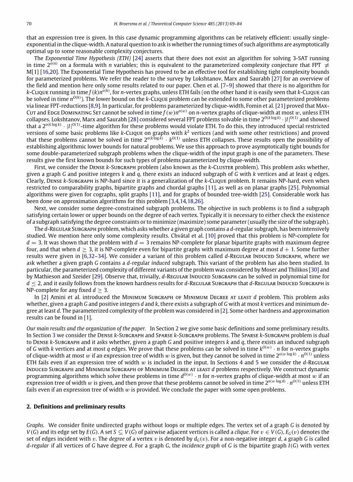
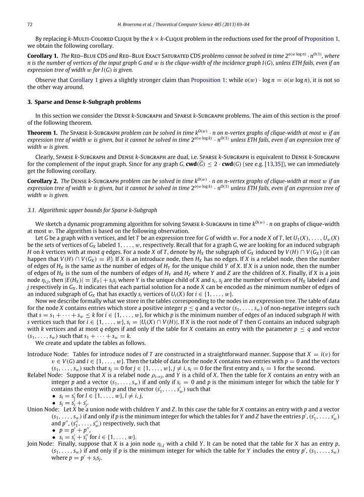
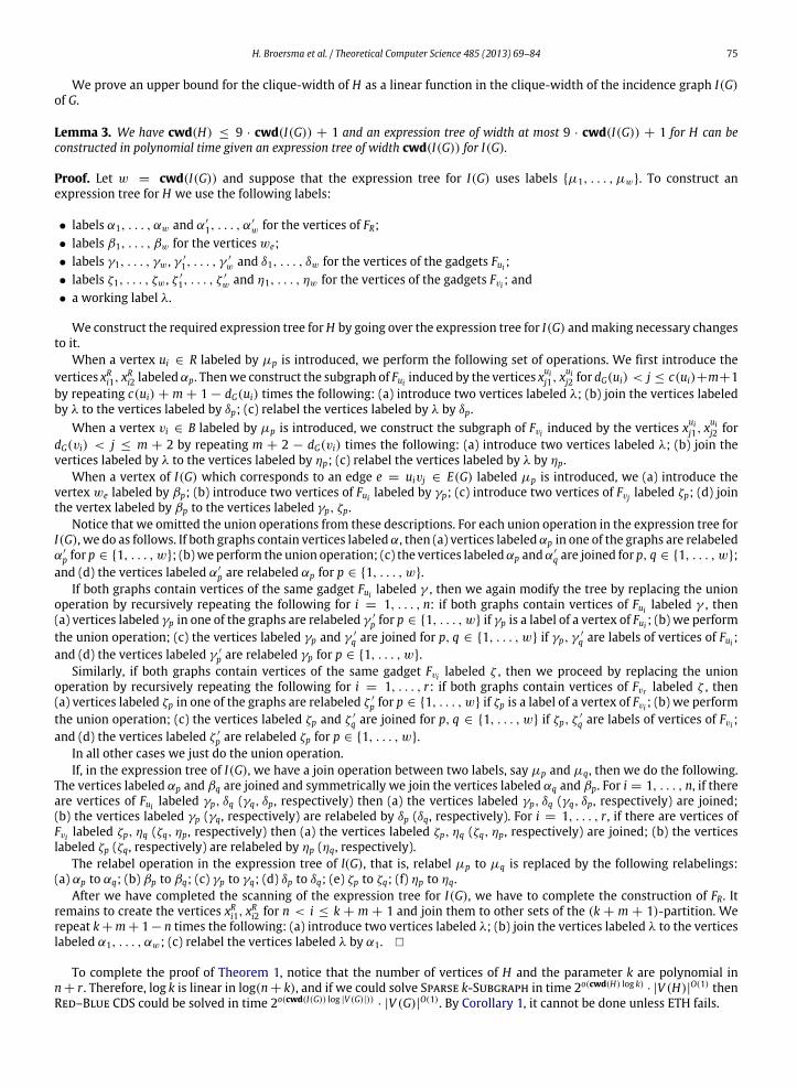
Fig. 1. Construction of H .
Correctness of the algorithm follows from the description of the procedure. Since for each X , the table for X contains atmost (k + 1)w vectors and for each vector only one value of the parameter p is stored, the algorithm runs in time kO(w)
· n.This proves that Sparse k-Subgraph can be solved in time kO(w)
· n on graphs of clique-width at most w.
3.2. Lower bounds
To prove our lower bounds we give a reduction from the Red–Blue CDS problem parameterized by the clique-width ofthe incidence graph of the input graph.
Construction. Let (G, c, k) be an instance of Red–Blue CDS with R = {u1, . . . , un} being the set of red vertices andB = {v1, . . . , vr} being the set of blue vertices. Letm be the number of edges of G. We assumewithout loss of generality thatG has no isolated vertices. Hence,m ≥ n, r .
First, we construct the auxiliary gadget F(l) for a positive integer l.
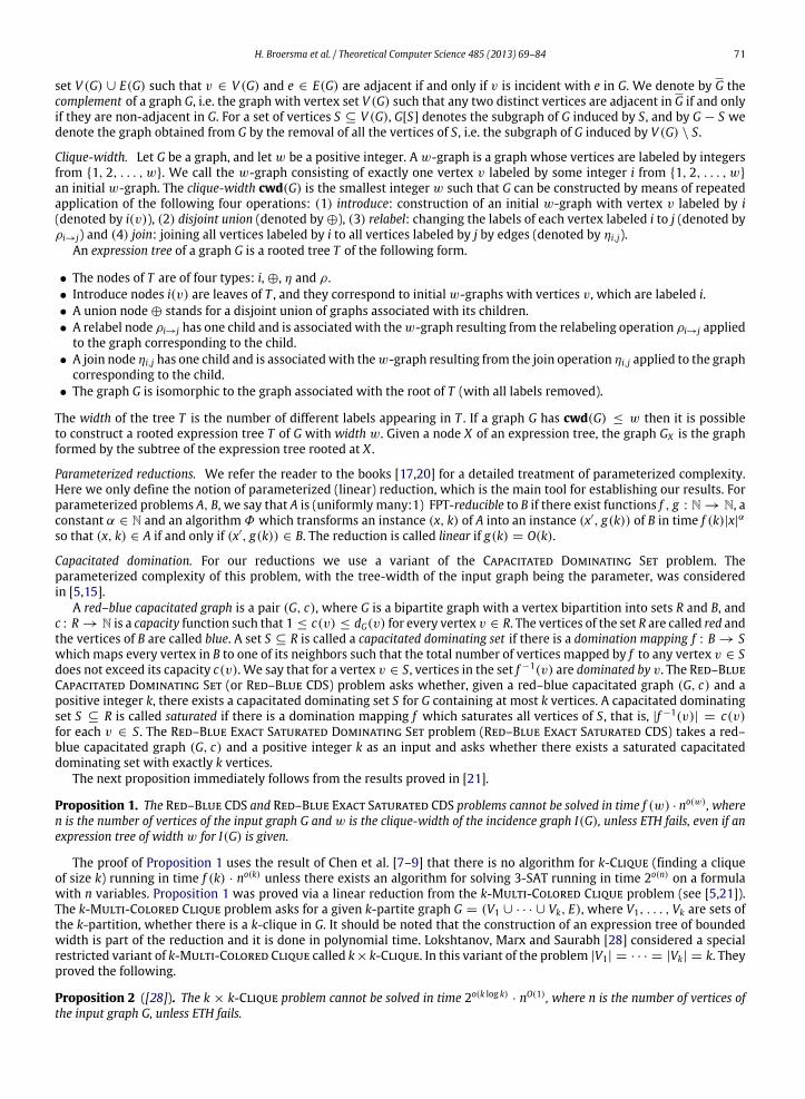
Auxiliary gadget F(l): Construct an l + m + 1-partite graph K2,...,2 and denote by xi1, xi2 the vertices of the i-th set of thepartition (see Fig. 1).
We need a technical lemma about properties of the gadget F(l).Lemma 1. Let J be a disjoint union of s copies F1, . . . , Fs of F(l1), . . . , F(ls), respectively for l1, . . . , ls ≥ 1, and let U ⊆ V (J).
• If |U| = 2s(m + 1) then |E(G[U])| ≥ 2sm(m + 1), and |E(G[U])| = 2sm(m + 1) if and only if U contains vertices of m + 1sets of the (li + m + 1)-partition of each copy of F(li).
• If |U| < 2s(m + 1) then 2sm(m + 1) − |E(G[U])| ≤ (2s(m + 1) − |U|) · 2m.• If |U| > 2s(m + 1) then |E(G[U])| − 2sm(m + 1) ≥ (|U| − 2s(m + 1)) · 2(m + 1).
Proof. For s = 1, the first claim follows immediately from the definition of F(l). Let s > 1. Suppose that U ⊆ V (J) contains2s(m + 1) vertices and the number of edges of J[U] is minimum. Let pi = V (Fi) ∩ U for i ∈ {1, . . . , s}. Since U induces asubgraph with the minimum number of edges, U contains vertices of ⌊pi/2⌋ sets of the (li + m + 1)-partition of each Fi.Assume that there are i, j ∈ {1, . . . , s} such that pi > 2(m+1) and pj < 2(m+1). Observe that there is a vertex u ∈ V (Fi)∩Uwhich is adjacent to at least 2(m+1) vertices ofU and there is a vertex v ∈ V (Fj)\U which is adjacent to atmost 2m verticesof U . Consider the set U ′
= (U \ {u}) ∪ {v}. Clearly, |E(J[U ′])| ≤ |E(J[U])| − 2(m + 1) + 2m < |E(J[U])|; this contradicts
our choice of U . Therefore pi = 2(m + 1).The second claim follows from the fact that if |U| < 2s(m+ 1) and G[U] has the minimum number of edges then we can
add 2s(m + 1) − |U| vertices of degree at most 2m. The third claim is proved by similar arguments. �
Reduction: Now we describe our reduction.
1. A copy of a gadget F(k) is constructed. Denote this graph by FR and let V (FR) = {xRi1, xRi2|1 ≤ i ≤ k + m + 1}.
2. For each i ∈ {1, . . . , n}, a copy of a gadget F(c(ui)) is created. Denote this graph by Fui and let V (Fui) = {xuij1, xuij2|1 ≤ j ≤
c(ui) + m + 1}.3. For each i ∈ {1, . . . , r}, a copy of a gadget F(1) is created. Denote this graph by Fvi and letV (Fvi) = {xvi
j1, xvij2|1 ≤ j ≤ m+2}.
4. For each e ∈ E(G), the vertex we is constructed.5. For each i ∈ {1, . . . , n}, let {e1, . . . , edi} = E(ui) for di = dG(ui). We consider the vertices we1 , . . . , wedi
; these verticesare joined by edges to the vertices xRi1, x
Ri2 of FR, and for each j ∈ {1, . . . , di}, wej is joined by edges to the vertices xuij1, x
uij2
of Fui .6. For each i ∈ {1, . . . , r}, let {e1, . . . , edi} = E(vi) for di = dG(vi). We consider the vertices we1 , . . . , wedi
and for eachj ∈ {1, . . . , di}, wej is joined by edges to the vertices xvi
j1, xvij2 of Fvi .
7. Create 2m + 1 vertices z1, . . . , z2m+1 and join them to all vertices we for e ∈ E(G).
Denote the obtained graph by H (see Fig. 1).The proof of correctness of the reduction is based on the next two lemmas.
Lemma 2. The red–blue graph G has a capacitated dominating set of size at most k if and only if H contains an induced subgraphwith 2(m + 1)(n + r + 1) + 2m + 1 + r vertices and at most 2m(m + 1)(n + r + 1) + r(2m + 1) edges.
74 H. Broersma et al. / Theoretical Computer Science 485 (2013) 69–84
Proof. Suppose that the red–blue graph G has a capacitated dominating set S of size at most k. Let f be a correspondingdomination mapping. We construct an induced subgraph Q of H as follows:
• Include all the vertices z1, . . . , z2m+1 in the set of vertices of Q .• For FR, selectm + 1 sets of the (k + m + 1)-partition {xRi1, x
Ri2} such that ui /∈ S and include these vertices in V (Q ).
• For each ui ∈ S, consider c ≤ c(ui) ≤ dG(ui) edges e1, . . . , ec ∈ E(ui) which are used for domination (i.e. for eachej = uivh, f (vh) = ui). Selectm + 1 sets of the (c(ui) + m + 1)-partition {xuij1, x
uij2} of Fui such that xuij1, x
uij2 are not adjacent
to we1 , . . . , wec and include these vertices in V (Q ).• For each ui ∈ R \ S, selectm+ 1 sets of the (c(ui) +m+ 1)-partition {xuij1, x
uij2} of Fui arbitrarily and include these vertices
in V (Q ).• For each vi ∈ B, let e = vif (vi) ∈ E(G). Select m + 1 sets of the (m + 2)-partition {xvi
j1, xvij2} of Fvi such that xvi
j1, xvij2 are not
adjacent to we and include these vertices in V (Q ).• For each vi ∈ B, include the vertex we for e = vif (vi) ∈ E(G) in Q .
It is straightforward to check that Q has 2m+ 1+ 2(m+ 1)(n+ r + 1) + r vertices and 2m(m+ 1)(n+ r + 1) + r(2m+ 1)edges.
Assume now that Q is an induced subgraph of H with 2(m + 1)(n + r + 1) + 2m + 1 + r vertices and the minimumnumber of edges, such that |E(Q )| ≤ 2m(m + 1)(n + r + 1) + r(2m + 1).
Claim 1. It can be assumed that z1, . . . , z2m+1 ∈ V (Q ).
Proof of Claim 1. Let Z = {z1, . . . , z2m+1} ∩ V (Q ) and suppose that |Z | < 2m+ 1. LetW = {we|e ∈ E(G)} ∩ V (Q ). Assumethat W = ∅. Suppose that |W | ≥ |Z |. Recall that m is the number of edges of G and, hence, |W | ≤ m. Then |Z | ≤ m and|{z1, . . . , z2m+1} \ Z | ≥ m + 1. Now we observe that the graph obtained from Q by the replacement of the vertices of Wby |W | vertices from {z1, . . . , z2m+1} \ Z contains less edges than Q and this contradicts our choice of Q . If |W | < |Z | thenthe graph obtained from Q by the replacement of a vertex u ∈ W by a vertex v ∈ {z1, . . . , z2m+1} \ Z has at most |E(Q )| −
|Z | + |W | − 1 < |E(Q )| edges and we again have a contradiction. Therefore W = ∅ and {z1, . . . , z2m+1} is an independentset in Q . Then the replacement of any 2m + 1 − |Z | vertices from V (Q ) \ Z by the vertices of {z1, . . . , z2m+1} \ Z does notincrease the number of edges. �
From now on we assume that z1, . . . , z2m+1 ∈ V (Q ).
Claim 2. The set V (Q ) contains 2(m+ 1)(n+ r + 1) vertices of the gadgets FR, Fu1 , . . . , Fun , Fv1 , . . . , Fvr and r vertices from theset {we|e ∈ E(G)}. Moreover, each of the gadgets FR, Fu1 , . . . , Fun , Fv1 , . . . , Fvr contains exactly 2(m + 1) vertices from m + 1sets of the partitions of the gadgets and the vertices from {we|e ∈ E(G)} ∩ V (Q ) are not adjacent to vertices of these gadgets inthe graph Q .
Proof of Claim 2. Let p be the number of vertices of Q in the gadgets FR, Fu1 , . . . , Fun , Fv1 , . . . , Fvr and let q be the numberof vertices in {we|e ∈ E(G)}.
Suppose that p < 2(m+1)(n+r+1). By the second claimof Lemma1,Q contains at least 2pm−2(n+r+1)(m+1)m edgesin the graphs FR, Fu1 , . . . , Fun , Fv1 , . . . , Fvr . Each of the q vertices we is adjacent to the vertices z1, . . . , z2m+1 in Q . Observethat p+q = 2(m+1)(n+r+1)+r . HenceQ contains at least 2m(m+1)(n+r+1)+(2m+1)m+(2(m+1)(n+r+1)−p) >2m(m + 1)(n + r + 1) + r(2m + 1) edges. This contradiction proves that p ≥ 2(m + 1)(n + r + 1).
Suppose now that p > 2(m + 1)(n + r + 1). We apply the third claim of Lemma 1 and conclude that Q has atleast (p − 2(n + r + 1)(m + 1))2(m + 1) + 2(n + r + 1)(m + 1)m = (r − q)2(m + 1) + 2(n + r + 1)(m + 1)medges. Recall that the q vertices we in Q are adjacent to the vertices z1, . . . , z2m+1 in Q . We have that Q contains at least(r−q)2(m+1)+2(n+r+1)(m+1)m+q(2m+1) = 2(n+r+1)(m+1)m+r(2m+1)+r−q > 2(n+r+1)(m+1)m+r(2m+1)edges. We conclude that p = 2(m + 1)(n + r + 1) and q = r .
Since p = 2(m+1)(n+ r +1) and q = r , Q has at most 2m(m+1)(n+ r +1) edges different fromwezj. By the first claimof Lemma 1, Q has at least 2m(m+ 1)(n+ r + 1) edges in the gadgets FR, Fu1 , . . . , Fun , Fv1 , . . . , Fvr . Hence the vertices from{we|e ∈ E(G)} ∩ V (Q ) are not adjacent to the vertices of these gadgets in the graph Q . Also by the same claim, each of thegadgets FR, Fu1 , . . . , Fun , Fv1 , . . . , Fvr contains exactly 2(m + 1) vertices of them + 1 sets of the partitions of the graph. �
Now we can complete the proof of the lemma.The graph Q has r vertices from the set {we|e ∈ E(G)}. Consider a gadget Fvi constructed for the vertex vi ∈ B. The
graph Q contains 2(m+ 1) vertices in Fvi which constitutem+ 1 sets in the (m+ 2)-partition of this graph. Hence only theunique vertex we, for e ∈ EG(vi), non-adjacent to the vertices of Fvi in Q can be included in V (Q ). It follows that for eachi ∈ {1, . . . , r}, exactly one vertex we is included in V (Q ). We define the mapping f : B → R by setting f (vi) = uj such thatwe ∈ V (Q ) for e = viuj. Now observe that 2(m+ 1) vertices of the graph FR inm+ 1 sets of the (k+m+ 1)-partition are inV (Q ). Thus, exactly k sets of vertices from {we|e ∈ EG(u1)}, . . . , {we|e ∈ EG(un)} are non-adjacent to all the vertices of FR inQ . We construct the set S ⊂ R by including in it vertices ui ∈ R for which {we|e ∈ EG(ui)} has this property. Clearly, |S| = k.Each we ∈ V (Q ) is included in one of the sets {we|e ∈ EG(ui)} for ui ∈ S. It remains to observe that each set {we|e ∈ EG(ui)}can only contain at most c(ui) vertices, namely those that are non-adjacent to the 2(m+1) vertices of Q in Fui . We concludethat S is a capacitated dominating set in the red–blue graph G and f is a dominating mapping for S. �
H. Broersma et al. / Theoretical Computer Science 485 (2013) 69–84 75
We prove an upper bound for the clique-width of H as a linear function in the clique-width of the incidence graph I(G)of G.
Lemma 3. We have cwd(H) ≤ 9 · cwd(I(G)) + 1 and an expression tree of width at most 9 · cwd(I(G)) + 1 for H can beconstructed in polynomial time given an expression tree of width cwd(I(G)) for I(G).
Proof. Let w = cwd(I(G)) and suppose that the expression tree for I(G) uses labels {µ1, . . . , µw}. To construct anexpression tree for H we use the following labels:
• labels α1, . . . , αw and α′
1, . . . , α′w for the vertices of FR;
• labels β1, . . . , βw for the vertices we;• labels γ1, . . . , γw , γ ′
1, . . . , γ′w and δ1, . . . , δw for the vertices of the gadgets Fui ;
• labels ζ1, . . . , ζw , ζ ′
1, . . . , ζ′w and η1, . . . , ηw for the vertices of the gadgets Fvi ; and
• a working label λ.
We construct the required expression tree forH by going over the expression tree for I(G) andmaking necessary changesto it.
When a vertex ui ∈ R labeled by µp is introduced, we perform the following set of operations. We first introduce thevertices xRi1, x
Ri2 labeledαp. Thenwe construct the subgraph of Fui induced by the vertices xuij1, x
uij2 for dG(ui) < j ≤ c(ui)+m+1
by repeating c(ui) + m + 1 − dG(ui) times the following: (a) introduce two vertices labeled λ; (b) join the vertices labeledby λ to the vertices labeled by δp; (c) relabel the vertices labeled by λ by δp.
When a vertex vi ∈ B labeled by µp is introduced, we construct the subgraph of Fvi induced by the vertices xuij1, xuij2 for
dG(vi) < j ≤ m + 2 by repeating m + 2 − dG(vi) times the following: (a) introduce two vertices labeled λ; (b) join thevertices labeled by λ to the vertices labeled by ηp; (c) relabel the vertices labeled by λ by ηp.
When a vertex of I(G) which corresponds to an edge e = uivj ∈ E(G) labeled µp is introduced, we (a) introduce thevertex we labeled by βp; (b) introduce two vertices of Fui labeled by γp; (c) introduce two vertices of Fvj labeled ζp; (d) jointhe vertex labeled by βp to the vertices labeled γp, ζp.
Notice that we omitted the union operations from these descriptions. For each union operation in the expression tree forI(G), we do as follows. If both graphs contain vertices labeledα, then (a) vertices labeledαp in one of the graphs are relabeledα′p for p ∈ {1, . . . , w}; (b)we perform the union operation; (c) the vertices labeledαp andα′
q are joined for p, q ∈ {1, . . . , w};and (d) the vertices labeled α′
p are relabeled αp for p ∈ {1, . . . , w}.If both graphs contain vertices of the same gadget Fui labeled γ , then we again modify the tree by replacing the union
operation by recursively repeating the following for i = 1, . . . , n: if both graphs contain vertices of Fui labeled γ , then(a) vertices labeled γp in one of the graphs are relabeled γ ′
p for p ∈ {1, . . . , w} if γp is a label of a vertex of Fui ; (b) we performthe union operation; (c) the vertices labeled γp and γ ′
q are joined for p, q ∈ {1, . . . , w} if γp, γ′q are labels of vertices of Fui ;
and (d) the vertices labeled γ ′p are relabeled γp for p ∈ {1, . . . , w}.
Similarly, if both graphs contain vertices of the same gadget Fvi labeled ζ , then we proceed by replacing the unionoperation by recursively repeating the following for i = 1, . . . , r: if both graphs contain vertices of Fvr labeled ζ , then(a) vertices labeled ζp in one of the graphs are relabeled ζ ′
p for p ∈ {1, . . . , w} if ζp is a label of a vertex of Fvi ; (b) we performthe union operation; (c) the vertices labeled ζp and ζ ′
q are joined for p, q ∈ {1, . . . , w} if ζp, ζ′q are labels of vertices of Fvi ;
and (d) the vertices labeled ζ ′p are relabeled ζp for p ∈ {1, . . . , w}.
In all other cases we just do the union operation.If, in the expression tree of I(G), we have a join operation between two labels, say µp and µq, then we do the following.
The vertices labeled αp and βq are joined and symmetrically we join the vertices labeled αq and βp. For i = 1, . . . , n, if thereare vertices of Fui labeled γp, δq (γq, δp, respectively) then (a) the vertices labeled γp, δq (γq, δp, respectively) are joined;(b) the vertices labeled γp (γq, respectively) are relabeled by δp (δq, respectively). For i = 1, . . . , r , if there are vertices ofFvi labeled ζp, ηq (ζq, ηp, respectively) then (a) the vertices labeled ζp, ηq (ζq, ηp, respectively) are joined; (b) the verticeslabeled ζp (ζq, respectively) are relabeled by ηp (ηq, respectively).
The relabel operation in the expression tree of l(G), that is, relabel µp to µq is replaced by the following relabelings:(a) αp to αq; (b) βp to βq; (c) γp to γq; (d) δp to δq; (e) ζp to ζq; (f) ηp to ηq.
After we have completed the scanning of the expression tree for I(G), we have to complete the construction of FR. Itremains to create the vertices xRi1, x
Ri2 for n < i ≤ k + m + 1 and join them to other sets of the (k + m + 1)-partition. We
repeat k+m+ 1− n times the following: (a) introduce two vertices labeled λ; (b) join the vertices labeled λ to the verticeslabeled α1, . . . , αw; (c) relabel the vertices labeled λ by α1. �
To complete the proof of Theorem 1, notice that the number of vertices of H and the parameter k are polynomial inn+ r . Therefore, log k is linear in log(n+ k), and if we could solve Sparse k-Subgraph in time 2o(cwd(H) log k)
· |V (H)|O(1) thenRed–Blue CDS could be solved in time 2o(cwd(I(G)) log |V (G)|))
· |V (G)|O(1). By Corollary 1, it cannot be done unless ETH fails.
76 H. Broersma et al. / Theoretical Computer Science 485 (2013) 69–84
4. Regular subgraph problem
In this section we consider the d-Regular Subgraph problem. The main aim is the proof of the following theorem.
Theorem 2. The d-Regular Induced Subgraph problem can be solved on n-vertex graphs of clique-width at most w in timedO(w)
· n if an expression tree of width w is given for the input graph, but it cannot be solved in time 2o(w log d)· nO(1) unless ETH
fails, even if an expression tree of width w is given.
The proof is given in the following two subsections.
4.1. Algorithmic upper bounds for d-Regular Induced Subgraph
We sketch a dynamic programming algorithm for solving d-Regular Induced Subgraph in time dO(w)· n on graphs of
clique-width at most w.Let G be a graph with n vertices, and let T be an expression tree for G of width w. Recall that for a node X of T , we
denote by GX the w-graph associated with this node. For a node X of T , let U1(X), . . . ,Uw(X) be the sets of vertices of GXlabeled 1, . . . , w, respectively. We are looking for an induced d-regular subgraph H of X . For a node X of T , denote by HX thesubgraph of GX induced by V (H) ∩ V (GX ) (it can happen that V (H) ∩ V (GX ) = ∅). We use the following observation.
If X is an introduce node, then HX has only vertices of degree 0 (or no vertices). If X is a relabel node, then the degreesof vertices of HX are the same as in HY for the unique child Y of X . If X is a union node, then the degree of HX are thedegrees of the corresponding vertices in HY and HZ where Y and Z are the children of X . Finally, if X is a join node ηi,j, thendHX (v) = dHY (v) + sj if v ∈ Ui(X) and dHX (v) = dHY (v) + si if v ∈ Uj(X) where Y is the unique child of X and si, sj are thenumber of vertices of HX labeled i and j respectively in GX . All other vertices have the same degrees as in GY . In particular, itimplies the following.
Observation 1. Let H be an induced d-regular subgraph of G. Then for any node X of the expression tree T , all vertices of HX fromthe set Ui(X) have the same degree (in H) for i ∈ {1, . . . , w}.
It indicates that each partial solution for a node X can be encoded by the degrees of vertices in each Ui(X) of an inducedsubgraph of GX that has exactly si vertices of Ui(X) for i ∈ {1, . . . , w}.
Nowwe describe formally what we store in the tables corresponding to the nodes in an expression tree. Let G be a graphwith n vertices and let T be an expression tree for G of width w. Recall that for a node X of T , we denote by GX the w-graphassociated with this node. We let U1(X), . . . ,Uw(X) be the sets of vertices of GX labeled 1, . . . , w respectively. The table ofdata for the node X stores pairs of integer vectors, (s1, . . . , sw) and (d1, . . . , dw), satisfying 0 ≤ si ≤ d + 1 and 0 ≤ di ≤ dfor all i ∈ {1, . . . , w}, and for which there is an induced subgraph H of GX such that for all i ∈ {1, . . . , w}
• di = dH(v) for all v ∈ V (H) ∩ Ui(X) (if V (H) ∩ Ui(X) = ∅ then it is assumed that this condition holds for all 0 ≤ di ≤ d),and
• si = min{|V (H) ∩ Ui(X)|, d + 1}.
If X is the root node of T (that is, G = GX ) then G contains a d-regular induced subgraph if and only if the table for X containsan entry with the vector (d1, . . . , dw) = (d, . . . , d).
Now we give the details of how we construct our tables and how we update them.
Introduce Node: Tables for introduce nodes of T are constructed in a straightforward manner. Suppose that X = i(v) forv ∈ V (G) and i ∈ {1, . . . , w}. Then the table of data for the node X contains the pairs of vectors (s1, . . . , sw) and(d1, . . . , dw) such that sj = 0 and 0 ≤ dj ≤ d for j ∈ {1, . . . , w}, j = i, and either si = 0 and 0 ≤ di ≤ d or si = 1and di = 0.
Relabel Node: Suppose that X is a relabel node ρi→j, and let Y be the child of X . Then the table for X contains a pair of vectors(s1, . . . , sw) and (d1, . . . , dw) if and only if si = 0, and the table for Y contains the entry (s′1, . . . , s
′w), (d′
1, . . . , d′w)
such that• sp = s′p and dp = d′
p for p ∈ {1, . . . , w}, p = i, j,• dj = d′
i = d′
j ,• sj = min{s′i + s′j, d + 1}.
Union Node: Let X be a union node with children Y and Z . In this case the table for X contains a pair of vectors (s1, . . . , sw)and (d1, . . . , dw) if and only if the tables for Y and Z have the pairs of vectors (s′1, . . . , s
′w), (d1, . . . , dw) and
(s′′1, . . . , s′′w), (d1, . . . , dw), respectively, such that si = min{s′i + s′′i , d + 1} for i ∈ {1, . . . , w}.
Join Node: Finally, suppose that X is a join node ηi,j with the child Y . The table for X has a pair of vectors (s1, . . . , sw) and(d1, . . . , dw) if and only if the table for Y includes a pair of vectors (s1, . . . , sw), (d′
1, . . . , d′w) such that
• d′p = dp for p ∈ {1, . . . , w}, p = i, j,
• di = d′
i + sj and dj = d′
j + si.
Correctness of the algorithm follows from the description and Observation 1. Since for each X , the table for X contains atmost (d + 2)2w pairs of vectors, the algorithm runs in time dO(w)
· n. This proves that d-Regular Induced Subgraph can besolved in time dO(w)
· n on graphs of clique-width at most w.
H. Broersma et al. / Theoretical Computer Science 485 (2013) 69–84 77
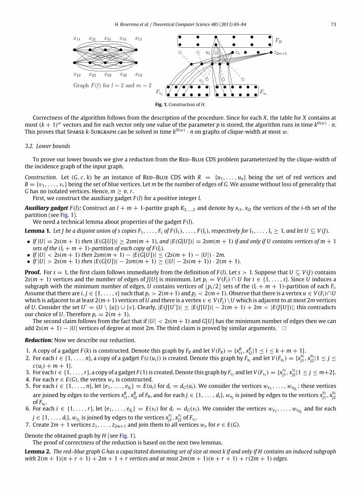
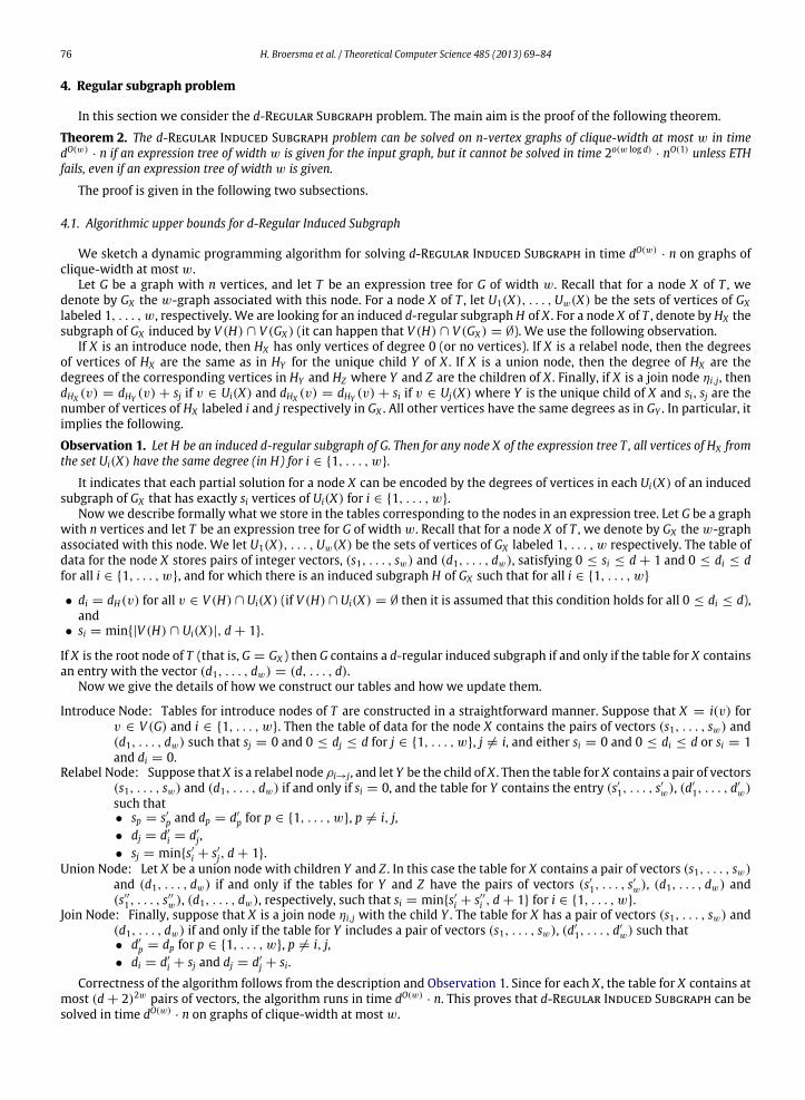
Fig. 2. Construction of H .
4.2. Algorithmic lower bounds for d-Regular Induced Subgraph
To prove our complexity lower bound, we give a reduction from the Red–Blue Exact Saturated CDS problem,parameterized by the clique-width of the incidence graph of the input graph, to the d-Regular Induced Subgraph problem.The proof is organized as follows: we first give a construction, then prove its correctness and finally bound the clique-widthof the transformed instance.
Construction. Let (G, c, k) be an instance of Red–Blue Exact Saturated CDS with R = {u1, . . . , un} being the set of redvertices and B = {v1, . . . , vr} being the set of blue vertices. Let d = n+ r +1 if n+ r is even and let d = n+ r +2 otherwise;notice that d is odd. We need an auxiliary gadget.
Auxiliary gadget F(x): Let x be a vertex.We construct d−12 copies of Kd+1, subdivide one edge of each copy, and glue (identify)
all these vertices of degree two into one vertex y. Finally we join x and y by an edge. We are going to attach gadgets F(x)to other parts of our construction through the vertex x. This vertex is called the root of F(x). The properties of F(x) that arerequired for our proof are summarized in the following simple lemma. The gadget F(x) for d = 5 is illustrated in Fig. 2.
Lemma 4.
• Let G′ be the graph obtained from a graph G with a vertex x by adding a copy of F(x). For any d-regular induced subgraph H ofG′, if any vertex of F(x) − x is included in H then V (F(x)) ⊆ V (H) and if x /∈ V (H) then V (F(x)) ∩ V (H) = ∅.
• We have cwd(F(x)) ≤ 4, and a 4-graph isomorphic to F(x) can be constructed in such a way that one label is used only forthe vertex x. Moreover it can be assumed that the construction starts from the vertex x with a given label α, and at the end allnon-root vertices are relabeled by a given label λ.
Proof. The first claim of the lemma follows immediately from the fact that all vertices of F(x) except x have degree d.To prove the second claim, let us note that F(x) is a cograph (i.e. a graph without induced paths on four vertices). It is
well-known that cographs have clique-width 2 (see e.g. [35]). It means that in fact cwd(F(x)) = 2. Clearly, by using twoadditional labels α and λ, we can get the desired 4-graph. �
Reduction: Now we describe our reduction. Recall that d = n + r + 1 if n + r is even and d = n + r + 2 otherwise. Lets = d − r − 1 and t = d − k − 1.
1. Vertices u1, . . . , un are created.2. A clique of size r with vertices v1, . . . , vr is constructed.3. For each edge e = uivj of G, a vertex we is added, joined by edges to ui and vj, and d − 2 copies of F(we) are constructed.4. A clique of size s with vertices a1, . . . , as is created, all vertices ai are joined to vertices v1, . . . , vr , and for each
i ∈ {1, . . . , s}, a copy of F(ai) is added.5. A vertex x is introduced and joined by edges to v1, . . . , vr and a1, . . . , as.6. A vertex y is added and joined by an edge to x, and k − 1 copies of F(y) are added.7. A clique of size t with vertices b1, . . . , bt is constructed, the vertex y is joined by edges to all vertices of the clique, and
for each j ∈ {1, . . . , t}, k copies of F(bi) are added.8. A vertex z is introduced and joined by edges to vertices y and b1, . . . , bt .9. For each i ∈ {1, . . . , n}, we let li = d − c(ui) − 1 and do the following:
– Add a vertex pi, join it to z by an edge, and construct c(ui) − 1 copies of F(pi).– Construct a clique of size li with vertices ci1, . . . , cili , join them to the vertex pi by edges, and for each j ∈ {1, . . . , li},
introduce c(ui) copies of F(cij).– Join the vertex ui to the vertices pi and ci1, . . . , cili by edges.
Denote the obtained graph by H . The construction of H is illustrated in Fig. 2.
Lemma 5. The red–blue graph G has an exact saturated capacitated dominating set of size k if and only if H contains an inducedd-regular subgraph.
78 H. Broersma et al. / Theoretical Computer Science 485 (2013) 69–84
Proof. Let S be an exact saturated capacitated dominating set of size k inG and let f be a corresponding dominationmapping.We construct an induced d-regular subgraph Q of H as follows:
• All the vertices v1, . . . , vr , a1, . . . , as, x, y, b1, . . . , bt and z are included in the set of vertices of Q .• For each ui ∈ S, all the vertices ui, ci1, . . . , cili and pi are included in the set of vertices of Q .• For each i ∈ {1, . . . , r}, the vertex we for e = vif (vi) ∈ E(G) is included in the set of vertices of Q .• For each gadget F(w) rooted at a vertex w ∈ V (H) such that w ∈ V (Q ), all the vertices of F(w) are included in Q .
It is straightforward to check that the subgraph of H induced by the vertices of Q is a d-regular graph.Assume now that Q is a d-regular induced subgraph of H . First we need some properties of Q .
Claim 3. All the vertices v1, . . . , vr , a1, . . . , as, x, y, b1, . . . , bt , z ∈ V (Q ).
Proof of Claim 3. Assume for the sake of contradiction that at least one vertex of the set {v1, . . . , vr , a1, . . . , as, x} is notin V (Q ). Then all the vertices a1, . . . , as, x, y are not in V (Q ) since they have degree d in H . Each vertex vi is adjacent toat most n vertices we and hence dH(vi) ≤ n + r + s ≤ d − 1 + s. Hence if a1, . . . , as /∈ V (Q ) then v1, . . . , vr /∈ V (Q ).Now we can conclude that all the vertices we cannot be vertices of Q and therefore u1, . . . , un /∈ V (Q ). Since y /∈ V (Q ),by the same arguments, b1, . . . , bt , z /∈ V (Q ), and if u1, . . . , un /∈ V (Q ) then all vertices pi and cij also cannot be includedin V (Q ). But this means that V (Q ) = ∅. We easily get the same conclusion if we assume that at least one vertex of the set{y, z, b1, . . . , bt} is not in V (Q ). �
Claim 4. There is a k-element set I ⊆ {1, . . . , n} such that for any i ∈ I , we have ui, ci1, . . . , cili , pi ∈ V (Q ), and for any i /∈ I ,we have ui, ci1, . . . , cili , pi /∈ V (Q ).
Proof of Claim 4. By Claim 3, we have y, b1, . . . , bt , z ∈ V (Q ). Hence z should be adjacent in Q to at least k other vertices,and therefore we have that exactly k vertices pi1 , . . . , pik ∈ V (Q ). Let I = {i1, . . . , ik}. It remains to observe that if pj ∈ V (Q )then pj, cj1, . . . , cjlj , uj ∈ V (Q ), and pj, cj1, . . . , cjlj , uj /∈ V (Q ) otherwise. �
By Claim 3, we have v1, . . . , vr , a1, . . . , as, x ∈ V (Q ). It follows that each vertex vi is adjacent to exactly one vertexwe in Q for some edge e = viuj ∈ E(G), and uj ∈ V (Q ) since dH(we) = d. By Claim 4, we have that exactly k verticesui1 , . . . , uik ∈ V (Q ). Also by this claim, uij , cij1, . . . , cij li , pij ∈ V (Q ) and hence each vertex uij should be adjacent to exactlyc(uij) verticeswe.We let S = {ui1 , . . . , uik} ⊆ R in the red–blue graphG anddefine amapping f : B → R by setting f (vi) = uj.It remains to observe that S is an exact saturated capacitated dominating set and f is a domination mapping for this set. �
Nowwe show that the clique-width of H is bounded from above by a linear function in the clique-width of the incidencegraph I(G) of G.
Lemma 6. We have that cwd(H) ≤ 3 · cwd(I(G)) + 6 and an expression tree of width at most 3 · cwd(I(G)) + 6 for H can beconstructed in polynomial time assuming we are given an expression tree of width cwd(I(G)) for I(G).
Proof. Letw = cwd(I(G)) and suppose that the expression tree for I(G) uses labels {α1, . . . , αw}. To construct an expressiontree for H we use the following additional labels:
• labels β1, . . . , βw and γ1, . . . , γw for the vertices v1, . . . , vr ;• a label δ for vertices pi;• working labels ζ1, ζ2 for the vertices a1, . . . , as, b1, . . . , bt , ci1, . . . , cili , x, y and z;• working labels η1, η2 for non-root vertices of gadgets F(w); and• a label λ for vertices of F(w) and for vertices that are not joined to other vertices in further stages of the construction.
We construct the required expression tree forH by going over the expression tree for I(G) andmaking necessary changesto it.
When a vertex ui ∈ R labeled by αp is introduced, we perform the following set of operations. We first introduce thevertex ui labeled αp. Then li vertices ci1, . . . , cili are created by repeating the following operations li times: (a) introduce avertex labeled ζ1; (b) join vertices labeled ζ1 to the vertices labeled αp and ζ2; (c) construct copies of F(cij) rooted at thisvertex using the labels η1, η2 as it is shown in Lemma 4 (recall that when a copy of F(ui) is constructed here and further,all the non-root vertices are relabeled by λ); (d) relabel vertices labeled ζ1 by ζ2. Finally, (a) the vertex pi labeled by δ1 isintroduced; (b) the vertex is joined to the vertices labeled αp and ζ2; (c) copies of F(pi) rooted at this vertex are constructed;(d) all the vertices labeled ζ2 are relabeled λ. We omit the union operations from our descriptions here and henceforth inany similar descriptions and assume that if some vertex is introduced then union is always performed.
When a vertex of I(G) that corresponds to an edge e ∈ E(G) labeled αp is introduced, we introduce the vertex we alsolabeled αp and add copies of F(we) rooted at this vertex.
When a vertex vi ∈ B labeled by αp is introduced, we introduce the vertex vi labeled βp.For each union operation in the expression tree for I(G), we do as follows. If both graphs contain vertices labeled β , then
(a) vertices labeled βp in one of the graphs are relabeled γp for p ∈ {1, . . . , w}; (b) we perform the union operation; (c) thevertices labeledβp and γq are joined for p, q ∈ {1, . . . , w}; and (d) the vertices labeled γp are relabeledβp for p ∈ {1, . . . , w}.If only one graph contains vertices labeled β then we just do the union operation.
H. Broersma et al. / Theoretical Computer Science 485 (2013) 69–84 79
If, in the expression tree of I(G), we have a join operation between two labels, say αp and αq, then we simulate this byapplying the join operations between the following: (a) αp and αq; (b) αp and βq; (c) βp and αq.
A relabel operation in the expression tree of I(G), say an operation relabeling αp to αq, is replaced by the followingrelabeling process: (a) αp to αq and (b) βp to βq.
After we have completed the scanning of the expression tree for I(G), we complete the construction of H . We createvertices a1, . . . , as by repeating the following operations s times: (a) introduce a vertex labeled ζ1; (b) join vertices labeledζ1 to the vertices labeled by labels βp for p ∈ {1, . . . , w} and ζ2; (c) construct copies of F(ai) rooted at this vertex usingthe labels η1, η2; (d) relabel vertices labeled ζ1 by ζ2. Then (a) the vertex x labeled by ζ1 is introduced; (b) it is joined toall the vertices labeled ζ2 and βp for p ∈ {1, . . . , w}; (c) all the vertices labeled ζ2 are relabeled by λ. Now (a) the vertex ylabeled by ζ2 is introduced; (b) copies of F(y) rooted at this vertex are added; (c) y is joined to the vertex x labeled ζ1; (c) allthe vertices labeled ζ1 are relabeled by λ. Then we create vertices b1, . . . , bt by repeating the following operations t times:(a) introduce a vertex labeled ζ1; (b) join vertices labeled ζ1 to vertices labeled ζ2; (c) construct copies of F(bi) rooted at thisvertex; (d) relabel vertices labeled ζ1 by ζ2. Finally we (a) introduce the vertex z labeled ζ1 and (b) join it to all the verticeslabeled by ζ2 or δ1. �
To conclude this part of the proof of Theorem 2, we observe that the number of vertices of H and the parameter d arepolynomial in n+ r , and therefore if we could solve d-Regular Induced Subgraph in time 2o(cwd(H) log d)
· |V (H)|O(1) then theRed–Blue Exact Saturated CDS could be solved in time 2o(cwd(I(G)) log |V (G)|))
· |V (G)|O(1). By Corollary 1, this cannot be doneunless ETH fails.
4.3. Variants of the d-Regular Induced Subgraph problem
We conclude this section by giving a corollary for some related problems. In the d-Regular Induced Subgraph problemwe ask about the existence of a d-regular induced subgraph for a given graph. It is possible to get similar results for somevariants of this problem. The Minimum d-Regular Induced Subgraph problem and the Maximum d-Regular InducedSubgraph problem are respectively the problems of finding a d-regular induced subgraph of minimum and maximum size.For the Counting d-Regular Induced Subgraph problem, we are interested in the number of induced d-regular subgraphsof the input graph. Using Theorem 2 we get the following corollary.Corollary 3. The Minimum d-Regular Induced Subgraph, Maximum d-Regular Induced Subgraph and Countingd-Regular Induced Subgraph problems can be solved on n-vertex graphs of clique-width at most w in time dO(w)
· n if anexpression tree of width w is given, but they cannot be solved in time 2o(w log d)
· nO(1) unless ETH fails, even if an expression treeof width w is given.Proof. To prove the algorithmic upper bounds, it is sufficient to modify the algorithm described for d-Regular InducedSubgraph. Particularly for Minimum d-Regular Induced Subgraph, each entry of the table of data for the node X shouldstore a positive integer p and pairs of vectors (s1, . . . , sw) and (d1, . . . , dw) of integers such that 0 ≤ si ≤ d + 1 and0 ≤ di ≤ d for i ∈ {1, . . . , w}, for which p is the number of vertices of an induced subgraph H of GX of minimum size suchthat for i ∈ {1, . . . , w}
• di = dH(v) for all v ∈ V (H) ∩ Ui(X) (observe that if V (H) ∩ Ui(X) = ∅ then it is assumed that this condition holds forany 0 ≤ di ≤ d), and
• si = min{|V (H) ∩ Ui(X)|, d + 1}.
For Maximum d-Regular Induced Subgraph and Counting d-Regular Induced Subgraph, the parameter p should be thenumber of vertices of an induced subgraph of maximum size and the number of subgraphs, respectively.
The lower bounds follow from Theorem 2 immediately. �
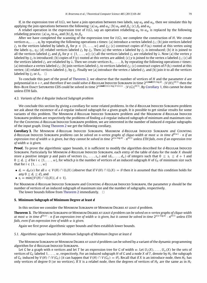
5. Minimum Subgraph of Minimum Degree at least d
In this section we consider theMinimum Subgraph of Minimum Degree at least d problem.Theorem 3. TheMinimum Subgraph ofMinimumDegree at least d problem can be solved on n-vertex graphs of clique-widthat most w in time dO(w)
· n if an expression tree of width w is given, but it cannot be solved in time 2o(w log d)· nO(1) unless ETH
fails, even if an expression tree of width w is given.Again we first prove algorithmic upper bounds and then establish lower bounds.
5.1. Algorithmic upper bounds for Minimum Subgraph of Minimum Degree at least d
TheMinimum Subgraph ofMinimumDegree at least d problem can be solved by a variant of the dynamic programmingalgorithm for d-Regular Induced Subgraph.
Let G be a graph with n vertices and let T be an expression tree for G of width w. Let U1(X), . . . ,Uw(X) be the sets ofvertices of GX labeled 1, . . . , w, respectively. For an induced subgraph H of G and a node X of T , denote by HX the subgraphof GX induced by V (H) ∩ V (GX ) (it can happen that V (H) ∩ V (GX ) = ∅). Recall that if X is an introduce node, then HX hasonly vertices of degree 0 (or no vertices). If X is a relabel node, then the degrees of vertices of HX are the same as in HY
80 H. Broersma et al. / Theoretical Computer Science 485 (2013) 69–84
for the unique child Y of X . If X is a union node, then the degree of HX are the degrees of the corresponding vertices in HYand HZ where Y and Z are the children of X . Finally, if X is a join node ηi,j, then dHX (v) = dHY (v) + sj if v ∈ Ui(X) anddHX (v) = dHY (v) + si if v ∈ Uj(X) where Y is the unique child of X and si, sj are the number of vertices of HX labeled i and jrespectively in GX . All other vertices have the same degrees as in GY . It shows that each partial solution for a node X can beencoded by the minimum degrees of vertices in each Ui(X) of an induced subgraph of GX that has exactly si vertices of Ui(X)for i ∈ {1, . . . , w}.
We describe formally what we store in the tables corresponding to the nodes in the expression tree. Let G be a graphwithn vertices and let T be an expression tree forG ofwidthw. LetU1(X), . . . ,Uw(X) be the sets of vertices ofGX labeled 1, . . . , w,respectively. Each entry of the table of data for the node X stores a positive integer p and pairs of vectors (s1, . . . , sw) and(d1, . . . , dw) of integers such that 0 ≤ si ≤ d and 0 ≤ di ≤ d for i ∈ {1, . . . , w}, for which p is the number of vertices of aninduced subgraph H of GX of minimum size such that for i ∈ {1, . . . , w}
• di = min{d,min{dH(v)|v ∈ V (H) ∩ Ui(X)}} (it is assumed that di = d if V (H) ∩ Ui(X) = ∅), and• si = min{|V (H) ∩ Ui(X)|, d}.
If X is the root node of T (that is, G = GX ) then G contains an induced subgraph of degree at least d with at most k verticesif and only if the table for X contains an entry with the parameter p ≤ k and vector (d1, . . . , dw) such that di ≥ d fori ∈ {1, . . . , w}.
Now we give the details of how we construct our tables and how we update them.
Introduce Node: Tables for introduce nodes of T are constructed in a straightforward manner. Suppose that X = i(v) forv ∈ V (G) and i ∈ {1, . . . , w}. Then the table of data for the node X contains the entries for p = 0 and p = 1.For p = 0, the table stores the pairs of vectors (s1, . . . , sw) and (d1, . . . , dw) such that sj = d and di = d forj ∈ {1, . . . , w}. For p = 1, the table contains the pairs of vectors (s1, . . . , sw) and (d1, . . . , dw) such that sj = dand di = d for j ∈ {1, . . . , w}, j = i, and si = 1, di = 0.
Relabel Node: Suppose that X is a relabel node ρi→j, and let Y be the child of X . Then the table for X contains an entry withan integer p and a pair of vectors (s1, . . . , sw) and (d1, . . . , dw) if and only if si = 0 and p is the minimum integerfor which the table for Y contains the entry with p and the vectors (s′1, . . . , s
′w), (d′
1, . . . , d′w) such that
• s′q = sq and d′q = dq for q ∈ {1, . . . , w}, q = i, j,
• di = min{d′
i, d′
j},• sj = min{s′i + s′j, d}.
Union Node: Let X be a union node with children Y and Z . In this case the table for X contains an entry with p and a pair ofvectors (s1, . . . , sw) and (d1, . . . , dw) if and only if p is the minimum integer for which the tables for Y and Z havethe entries p′, (s′1, . . . , s
′w), (d′
1, . . . , d′w) and p′′, (s′′1, . . . , s
′′w), (d′′
1, . . . , d′′w), respectively, such that
• p = p′+ p′′,
• di = min{d′
i, d′′
i } for i ∈ {1, . . . , w}, and• si = min{s′i + s′′i , d} for i ∈ {1, . . . , w}.
Join Node: Finally, suppose that X is a join node ηi,j with the child Y . It can be noted that the table for X has an entry p,(s1, . . . , sw), (d1, . . . , dw) if and only if p is the minimum integer for which the table for Y includes the entry p,(s1, . . . , sw), (d′
1, . . . , d′w) such that
• d′q = dq for q ∈ {1, . . . , w}, q = i, j,
• di = min{d′
i + sj, d} and dj = min{d′
j + si, d}.
Correctness of the algorithm follows from the description of the procedure.Since for each X , the table for X contains at most (d + 1)2w pairs of vectors and for each pair of vectors only one value of
the parameter p is stored, the algorithm runs in time dO(w)· n. This proves thatMinimum Subgraph of Minimum Degree at
least d can be solved in time dO(w)· n on graphs of clique-width at most w.
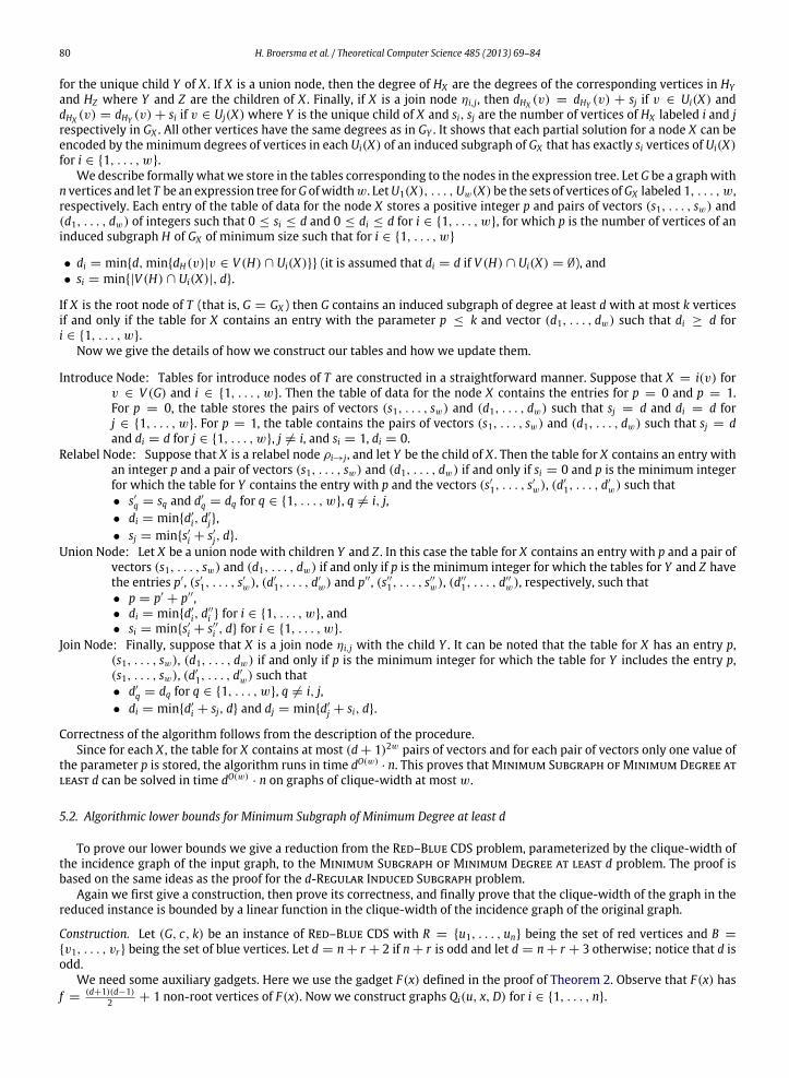
5.2. Algorithmic lower bounds for Minimum Subgraph of Minimum Degree at least d
To prove our lower bounds we give a reduction from the Red–Blue CDS problem, parameterized by the clique-width ofthe incidence graph of the input graph, to the Minimum Subgraph of Minimum Degree at least d problem. The proof isbased on the same ideas as the proof for the d-Regular Induced Subgraph problem.
Again we first give a construction, then prove its correctness, and finally prove that the clique-width of the graph in thereduced instance is bounded by a linear function in the clique-width of the incidence graph of the original graph.
Construction. Let (G, c, k) be an instance of Red–Blue CDS with R = {u1, . . . , un} being the set of red vertices and B =
{v1, . . . , vr} being the set of blue vertices. Let d = n + r + 2 if n + r is odd and let d = n + r + 3 otherwise; notice that d isodd.
We need some auxiliary gadgets. Here we use the gadget F(x) defined in the proof of Theorem 2. Observe that F(x) hasf =
(d+1)(d−1)2 + 1 non-root vertices of F(x). Now we construct graphs Qi(u, x,D) for i ∈ {1, . . . , n}.
H. Broersma et al. / Theoretical Computer Science 485 (2013) 69–84 81
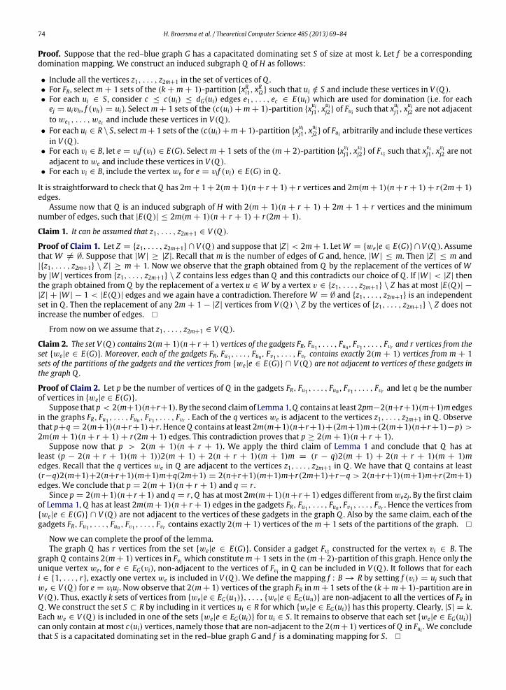
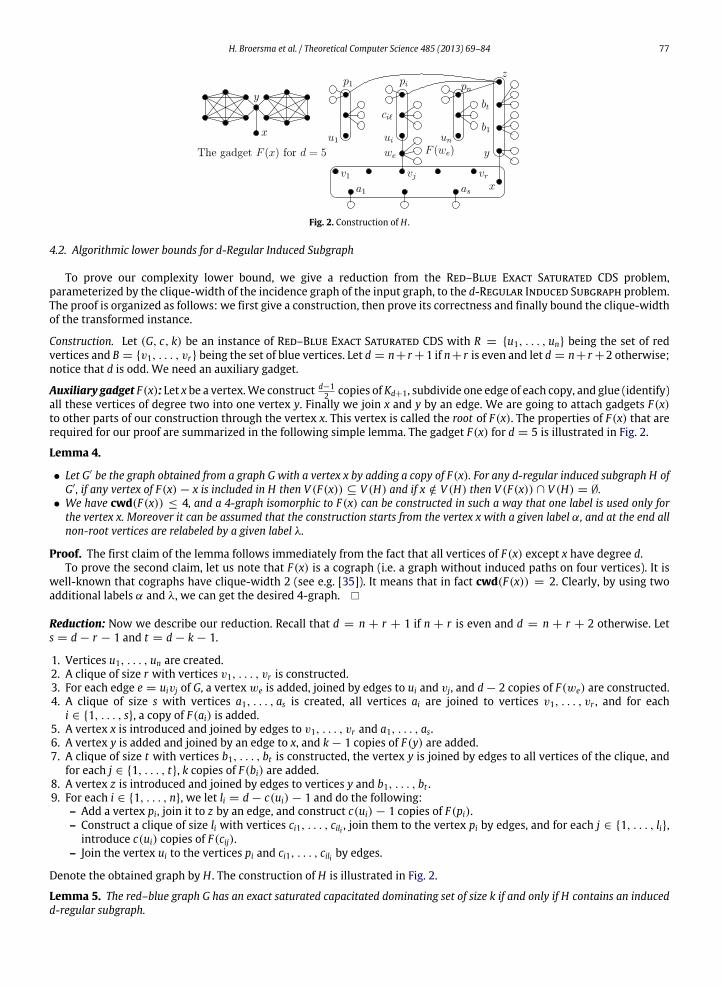
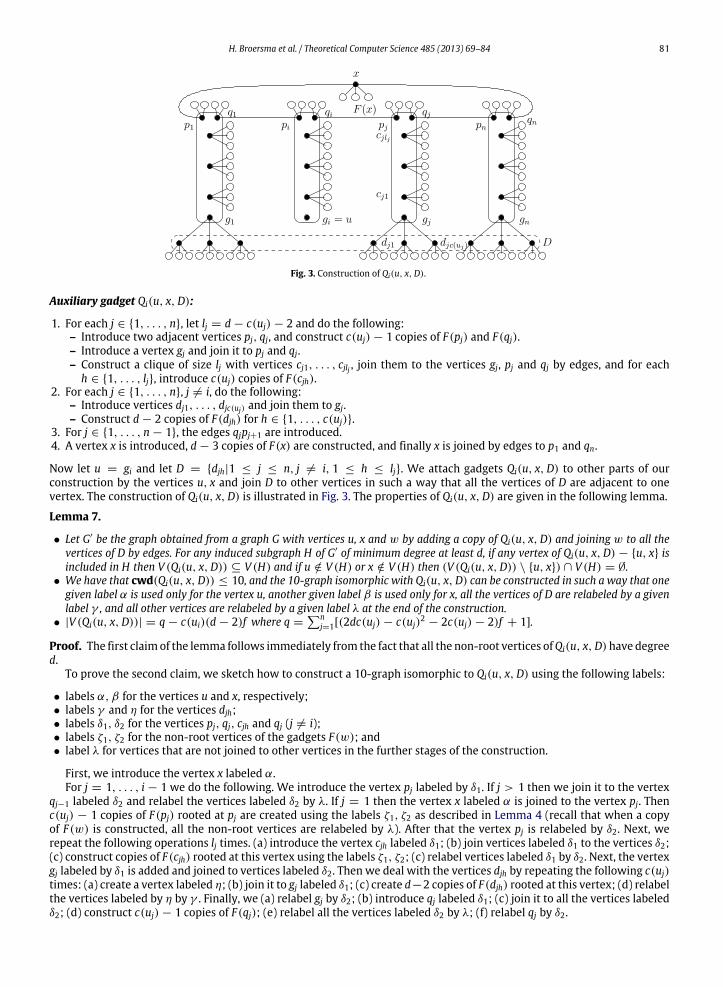
Fig. 3. Construction of Qi(u, x,D).
Auxiliary gadget Qi(u, x,D):
1. For each j ∈ {1, . . . , n}, let lj = d − c(uj) − 2 and do the following:– Introduce two adjacent vertices pj, qj, and construct c(uj) − 1 copies of F(pj) and F(qj).– Introduce a vertex gj and join it to pj and qj.– Construct a clique of size lj with vertices cj1, . . . , cjlj , join them to the vertices gj, pj and qj by edges, and for each
h ∈ {1, . . . , lj}, introduce c(uj) copies of F(cjh).2. For each j ∈ {1, . . . , n}, j = i, do the following:
– Introduce vertices dj1, . . . , djc(uj) and join them to gj.– Construct d − 2 copies of F(djh) for h ∈ {1, . . . , c(uj)}.
3. For j ∈ {1, . . . , n − 1}, the edges qjpj+1 are introduced.4. A vertex x is introduced, d − 3 copies of F(x) are constructed, and finally x is joined by edges to p1 and qn.
Now let u = gi and let D = {djh|1 ≤ j ≤ n, j = i, 1 ≤ h ≤ lj}. We attach gadgets Qi(u, x,D) to other parts of ourconstruction by the vertices u, x and join D to other vertices in such a way that all the vertices of D are adjacent to onevertex. The construction of Qi(u, x,D) is illustrated in Fig. 3. The properties of Qi(u, x,D) are given in the following lemma.
Lemma 7.
• Let G′ be the graph obtained from a graph G with vertices u, x and w by adding a copy of Qi(u, x,D) and joining w to all thevertices of D by edges. For any induced subgraph H of G′ of minimum degree at least d, if any vertex of Qi(u, x,D) − {u, x} isincluded in H then V (Qi(u, x,D)) ⊆ V (H) and if u /∈ V (H) or x /∈ V (H) then (V (Qi(u, x,D)) \ {u, x}) ∩ V (H) = ∅.
• We have that cwd(Qi(u, x,D)) ≤ 10, and the 10-graph isomorphic with Qi(u, x,D) can be constructed in such a way that onegiven label α is used only for the vertex u, another given label β is used only for x, all the vertices of D are relabeled by a givenlabel γ , and all other vertices are relabeled by a given label λ at the end of the construction.
• |V (Qi(u, x,D))| = q − c(ui)(d − 2)f where q =n
j=1[(2dc(uj) − c(uj)2− 2c(uj) − 2)f + 1].
Proof. The first claimof the lemma follows immediately from the fact that all the non-root vertices ofQi(u, x,D)have degreed.
To prove the second claim, we sketch how to construct a 10-graph isomorphic to Qi(u, x,D) using the following labels:
• labels α, β for the vertices u and x, respectively;• labels γ and η for the vertices djh;• labels δ1, δ2 for the vertices pj, qj, cjh and qj (j = i);• labels ζ1, ζ2 for the non-root vertices of the gadgets F(w); and• label λ for vertices that are not joined to other vertices in the further stages of the construction.
First, we introduce the vertex x labeled α.For j = 1, . . . , i − 1 we do the following. We introduce the vertex pj labeled by δ1. If j > 1 then we join it to the vertex
qj−1 labeled δ2 and relabel the vertices labeled δ2 by λ. If j = 1 then the vertex x labeled α is joined to the vertex pj. Thenc(uj) − 1 copies of F(pj) rooted at pj are created using the labels ζ1, ζ2 as described in Lemma 4 (recall that when a copyof F(w) is constructed, all the non-root vertices are relabeled by λ). After that the vertex pj is relabeled by δ2. Next, werepeat the following operations lj times. (a) introduce the vertex cjh labeled δ1; (b) join vertices labeled δ1 to the vertices δ2;(c) construct copies of F(cjh) rooted at this vertex using the labels ζ1, ζ2; (c) relabel vertices labeled δ1 by δ2. Next, the vertexgj labeled by δ1 is added and joined to vertices labeled δ2. Then we deal with the vertices djh by repeating the following c(uj)times: (a) create a vertex labeled η; (b) join it to gj labeled δ1; (c) create d−2 copies of F(djh) rooted at this vertex; (d) relabelthe vertices labeled by η by γ . Finally, we (a) relabel gj by δ2; (b) introduce qj labeled δ1; (c) join it to all the vertices labeledδ2; (d) construct c(uj) − 1 copies of F(qj); (e) relabel all the vertices labeled δ2 by λ; (f) relabel qj by δ2.
82 H. Broersma et al. / Theoretical Computer Science 485 (2013) 69–84
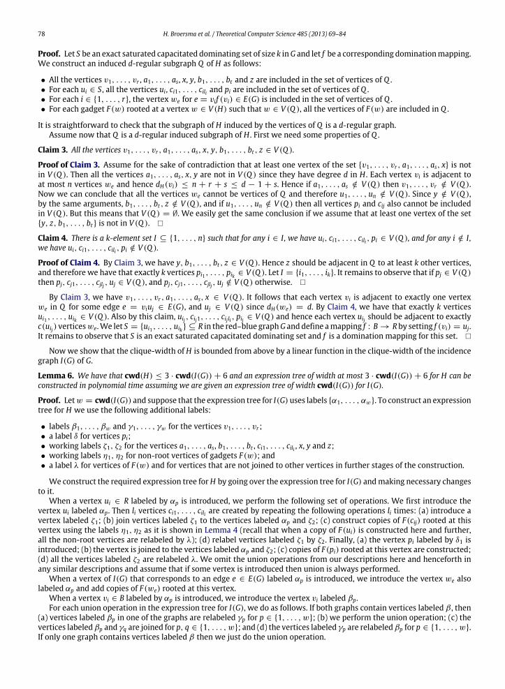
Fig. 4. Construction of H .
For j = i, we use almost the same operations. The only differences are that we label u = gi by β , we do not relabel it, wedo not repeat the operations described above for djh, and finally we join qi to the vertex labeled β . For j = i + 1, . . . , n, ourconstruction is the same as for j ∈ {1, . . . , i− 1}. The construction is concluded by joining x labeled by α to qn labeled by γ2and relabeling qn by λ.
The third claim of the lemma follows immediately from the description of Qi(u, x,D). �
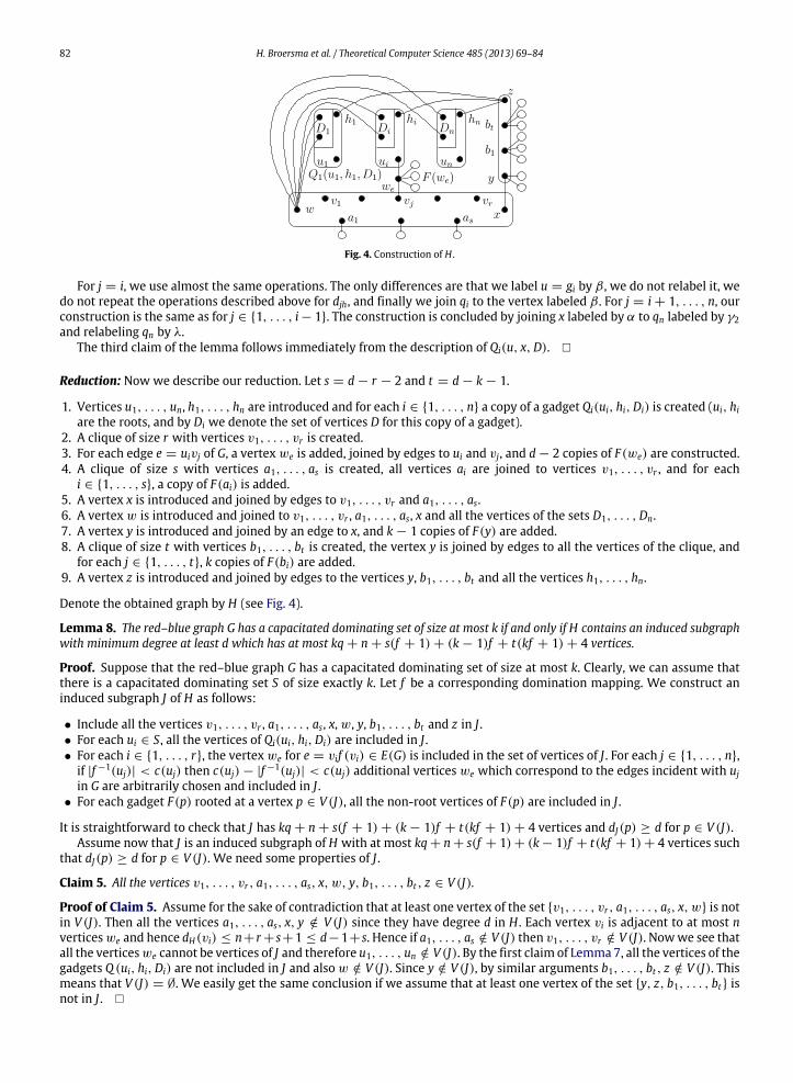
Reduction: Now we describe our reduction. Let s = d − r − 2 and t = d − k − 1.
1. Vertices u1, . . . , un, h1, . . . , hn are introduced and for each i ∈ {1, . . . , n} a copy of a gadget Qi(ui, hi,Di) is created (ui, hiare the roots, and by Di we denote the set of vertices D for this copy of a gadget).
2. A clique of size r with vertices v1, . . . , vr is created.3. For each edge e = uivj of G, a vertex we is added, joined by edges to ui and vj, and d − 2 copies of F(we) are constructed.4. A clique of size s with vertices a1, . . . , as is created, all vertices ai are joined to vertices v1, . . . , vr , and for each
i ∈ {1, . . . , s}, a copy of F(ai) is added.5. A vertex x is introduced and joined by edges to v1, . . . , vr and a1, . . . , as.6. A vertex w is introduced and joined to v1, . . . , vr , a1, . . . , as, x and all the vertices of the sets D1, . . . ,Dn.7. A vertex y is introduced and joined by an edge to x, and k − 1 copies of F(y) are added.8. A clique of size t with vertices b1, . . . , bt is created, the vertex y is joined by edges to all the vertices of the clique, and
for each j ∈ {1, . . . , t}, k copies of F(bi) are added.9. A vertex z is introduced and joined by edges to the vertices y, b1, . . . , bt and all the vertices h1, . . . , hn.
Denote the obtained graph by H (see Fig. 4).
Lemma 8. The red–blue graph G has a capacitated dominating set of size at most k if and only if H contains an induced subgraphwith minimum degree at least d which has at most kq + n + s(f + 1) + (k − 1)f + t(kf + 1) + 4 vertices.
Proof. Suppose that the red–blue graph G has a capacitated dominating set of size at most k. Clearly, we can assume thatthere is a capacitated dominating set S of size exactly k. Let f be a corresponding domination mapping. We construct aninduced subgraph J of H as follows:
• Include all the vertices v1, . . . , vr , a1, . . . , as, x, w, y, b1, . . . , bt and z in J .• For each ui ∈ S, all the vertices of Qi(ui, hi,Di) are included in J .• For each i ∈ {1, . . . , r}, the vertex we for e = vif (vi) ∈ E(G) is included in the set of vertices of J . For each j ∈ {1, . . . , n},
if |f −1(uj)| < c(uj) then c(uj) − |f −1(uj)| < c(uj) additional vertices we which correspond to the edges incident with ujin G are arbitrarily chosen and included in J .
• For each gadget F(p) rooted at a vertex p ∈ V (J), all the non-root vertices of F(p) are included in J .
It is straightforward to check that J has kq + n + s(f + 1) + (k − 1)f + t(kf + 1) + 4 vertices and dJ(p) ≥ d for p ∈ V (J).Assume now that J is an induced subgraph of H with at most kq + n + s(f + 1) + (k − 1)f + t(kf + 1) + 4 vertices such
that dJ(p) ≥ d for p ∈ V (J). We need some properties of J .
Claim 5. All the vertices v1, . . . , vr , a1, . . . , as, x, w, y, b1, . . . , bt , z ∈ V (J).
Proof of Claim 5. Assume for the sake of contradiction that at least one vertex of the set {v1, . . . , vr , a1, . . . , as, x, w} is notin V (J). Then all the vertices a1, . . . , as, x, y /∈ V (J) since they have degree d in H . Each vertex vi is adjacent to at most nverticeswe and hence dH(vi) ≤ n+ r+ s+1 ≤ d−1+ s. Hence if a1, . . . , as /∈ V (J) then v1, . . . , vr /∈ V (J). Nowwe see thatall the verticeswe cannot be vertices of J and therefore u1, . . . , un /∈ V (J). By the first claim of Lemma 7, all the vertices of thegadgets Q (ui, hi,Di) are not included in J and also w /∈ V (J). Since y /∈ V (J), by similar arguments b1, . . . , bt , z /∈ V (J). Thismeans that V (J) = ∅. We easily get the same conclusion if we assume that at least one vertex of the set {y, z, b1, . . . , bt} isnot in J . �
H. Broersma et al. / Theoretical Computer Science 485 (2013) 69–84 83
Claim 6. There is a k-element set I ⊆ {1, . . . , n} such that for any i ∈ I , V (Qi(ui, hi,Di)) ⊆ V (J), and for any i /∈ I , none of thevertices of Qi(ui, hi,Di) is included in J.Proof of Claim 6. By Claim 5, y, b1, . . . , bt , z ∈ V (J). Hence z is adjacent in J to at least k other vertices, and therefore thereare k′
≥ k vertices hi1 , . . . , hik′ in V (J). By the first claim of Lemma 7, all the vertices of Qij(uij , hij ,Dij) for j ∈ {1, . . . , k′} are
in J . Nowwe observe that for each j ∈ {1, . . . , k′}, at least c(uij) vertices we adjacent to uij should be included in J . Using the
third claim of Lemma 7, we conclude that J has at least k′q + n + s(f + 1) + (k − 1)f + t(kf + 1) + 4 vertices. So, k′= k
and we let I = {i1, . . . , ik′}. �
Now we complete the proof of the lemma. By Claim 5, we have that v1, . . . , vr , a1, . . . , as, x ∈ V (J). It follows that eachvertex vi is adjacent to at least one vertex we in J for some edge e = viuj ∈ E(G), and uj ∈ V (J) since dH(we) = d. We definea mapping f : B → R by setting f (vi) = uj. By Claim 6, exactly k vertices ui1 , . . . , uik ∈ V (J). We let S = {ui1 , . . . , uik} ⊆ Rin the red–blue graph G. Also by this claim, all the vertices of Qi1(ui1 , hi1 ,Di1), . . . ,Qik(uik , hik ,Dik) are included in V (J), andhence each vertex uij should be adjacent to at least c(uij) vertices we. Observe that if there is a vertex uij which is adjacentto more than c(uij) vertices we, then |V (J)| > kq + n + s(f + 1) + (k − 1)f + t(kf + 1) + 4. Therefore each vertex uij isadjacent to exactly c(uij) vertices we. This means that S is a capacitated dominating set and f is a domination mapping forthis set. �
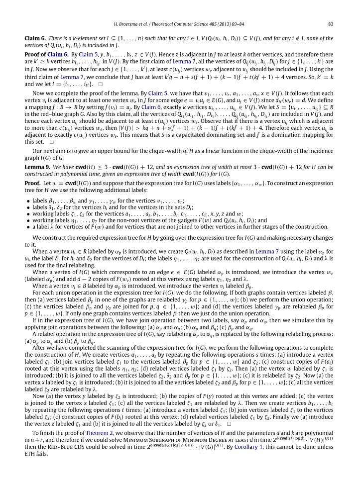
Our next aim is to give an upper bound for the clique-width of H as a linear function in the clique-width of the incidencegraph I(G) of G.Lemma 9. We have cwd(H) ≤ 3 · cwd(I(G)) + 12, and an expression tree of width at most 3 · cwd(I(G)) + 12 for H can beconstructed in polynomial time, given an expression tree of width cwd(I(G)) for I(G).Proof. Letw = cwd(I(G)) and suppose that the expression tree for I(G) uses labels {α1, . . . , αw}. To construct an expressiontree for H we use the following additional labels:
• labels β1, . . . , βw and γ1, . . . , γw for the vertices v1, . . . , vr ;• labels δ1, δ2 for the vertices hi and for the vertices in the sets Di;• working labels ζ1, ζ2 for the vertices a1, . . . , as, b1, . . . , bt , ci1, . . . , cili , x, y, z and w;• working labels η1, . . . , η7 for the non-root vertices of the gadgets F(w) and Qi(ui, hi,Di); and• a label λ for vertices of F(w) and for vertices that are not joined to other vertices in further stages of the construction.
We construct the required expression tree forH by going over the expression tree for I(G) andmaking necessary changesto it.
When a vertex ui ∈ R labeled by αp is introduced, we create Qi(ui, hi,Di) as described in Lemma 7 using the label αp forui, the label δ1 for hi and δ2 for the vertices of Di; the labels η1, . . . , η7 are used for the construction of Qi(ui, hi,Di) and λ isused for the final relabeling.
When a vertex of I(G) which corresponds to an edge e ∈ E(G) labeled αp is introduced, we introduce the vertex we(labeled αp) and add d − 2 copies of F(we) rooted at this vertex using labels η1, η2 and λ.
When a vertex vi ∈ B labeled by αp is introduced, we introduce the vertex vi labeled βp.For each union operation in the expression tree for I(G), we do the following. If both graphs contain vertices labeled β ,
then (a) vertices labeled βp in one of the graphs are relabeled γp for p ∈ {1, . . . , w}; (b) we perform the union operation;(c) the vertices labeled βp and γq are joined for p, q ∈ {1, . . . , w}; and (d) the vertices labeled γp are relabeled βp forp ∈ {1, . . . , w}. If only one graph contains vertices labeled β then we just do the union operation.
If in the expression tree of I(G), we have join operation between two labels, say αp and αq, then we simulate this byapplying join operations between the following: (a) αp and αq; (b) αp and βq; (c) βp and αq.
A relabel operation in the expression tree of I(G), say relabeling αp to αq, is replaced by the following relabeling process:(a) αp to αq and (b) βp to βq.
After we have completed the scanning of the expression tree for I(G), we perform the following operations to completethe construction of H . We create vertices a1, . . . , as by repeating the following operations s times: (a) introduce a vertexlabeled ζ1; (b) join vertices labeled ζ1 to the vertices labeled βp for p ∈ {1, . . . , w} and ζ2; (c) construct copies of F(ai)rooted at this vertex using the labels η1, η2; (d) relabel vertices labeled ζ1 by ζ2. Then (a) the vertex w labeled by ζ1 isintroduced; (b) it is joined to all the vertices labeled ζ2, δ2 and βp for p ∈ {1, . . . , w}; (c) it is relabeled by ζ2. Now (a) thevertex x labeled by ζ1 is introduced; (b) it is joined to all the vertices labeled ζ2 and βp for p ∈ {1, . . . , w}; (c) all the verticeslabeled ζ2 are relabeled by λ.
Now (a) the vertex y labeled by ζ2 is introduced; (b) the copies of F(y) rooted at this vertex are added; (c) the vertexis joined to the vertex x labeled ζ1; (c) all the vertices labeled ζ1 are relabeled by λ. Then we create vertices b1, . . . , btby repeating the following operations t times: (a) introduce a vertex labeled ζ1; (b) join vertices labeled ζ1 to the verticeslabeled ζ2; (c) construct copies of F(bi) rooted at this vertex; (d) relabel vertices labeled ζ1 by ζ2. Finally we (a) introducethe vertex z labeled ζ1 and (b) it is joined to all the vertices labeled by ζ2 or δ1. �
To finish the proof of Theorem 2, we observe that the number of vertices of H and the parameters d and k are polynomialin n+ r , and therefore if we could solveMinimum Subgraph ofMinimumDegree at least d in time 2o(cwd(H) log d)
· |V (H)|O(1)
then the Red–Blue CDS could be solved in time 2o(cwd(I(G)) log |V (G)|))· |V (G)|O(1). By Corollary 1, this cannot be done unless
ETH fails.
84 H. Broersma et al. / Theoretical Computer Science 485 (2013) 69–84
6. Conclusion
We established tight algorithmic lower and upper bounds for some double-parameterized subgraph problems when theclique-width of the input graph is one of the parameters. We believe that similar bounds could be given for other problems.
Another interesting task is to consider problems parameterized by other width-parameters. Throughout the paper, in allour results we assumed that an expression tree of the given width is part of the input. This is crucial, since – unlike the caseof tree-width – to date we are unaware of an efficient (FPT or polynomial) algorithm for computing an expression tree witha constant factor approximation of the clique-width. The algorithm given by Oum and Seymour in [31] provides a constantfactor approximation for another graph parameter – rank-width [23,31]. Hence, it is natural to ask whether it is possibleto establish tight algorithmic bounds for Dense k-Subgraph, d-Regular Induced Subgraph and Minimum Subgraph ofMinimum Degree at least d parameterized by the rank-width of the input graph. Also it would be interesting to considerproblems parameterized by the tree-width. For example, it can be shown that d-Regular Induced Subgraph andMinimumSubgraph of Minimum Degree at least d can be solved in time dO(t)
· n for n-vertex graphs of tree-width at most t . Is thisbound asymptotically tight?
Acknowledgment
The second author was supported by the European Research Council (ERC) via grant Rigorous Theory of Preprocessing,reference 267959.
References
[1] O. Amini, D. Peleg, S. Pérennes, I. Sau, S. Saurabh, On the approximability of some degree-constrained subgraph problems, Discrete Appl. Math. 160(2012) 1661–1679.
[2] O. Amini, I. Sau, S. Saurabh, Parameterized complexity of finding small degree-constrained subgraphs, J. Discrete Algorithms 10 (2012) 70–83.[3] S. Arora, D.R. Karger, M. Karpinski, Polynomial time approximation schemes for dense instances of NP-hard problems, J. Comput. Syst. Sci. 58 (1999)
193–210.[4] Y. Asahiro, K. Iwama, H. Tamaki, T. Tokuyama, Greedily finding a dense subgraph, J. Algorithms 34 (2000) 203–221.[5] H. L. Bodlaender, D. Lokshtanov, E. Penninkx, Planar capacitated dominating set is W [1]-hard, in: IWPEC, in: Lecture Notes in Computer Science,
vol. 5917, Springer, 2009, pp. 50–60.[6] F. Cheah, D.G. Corneil, The complexity of regular subgraph recognition, Discrete Appl. Math. 27 (1990) 59–68.[7] J. Chen, B. Chor, M. Fellows, X. Huang, D. Juedes, I.A. Kanj, G. Xia, Tight lower bounds for certain parameterized NP-hard problems, Inform. and Comput.
201 (2005) 216–231.[8] J. Chen, X. Huang, I.A. Kanj, G. Xia, On the computational hardness based on linear FPT-reductions, J. Comb. Optim. 11 (2006) 231–247.[9] J. Chen, X. Huang, I.A. Kanj, G. Xia, Strong computational lower bounds via parameterized complexity, J. Comput. Syst. Sci. 72 (2006) 1346–1367.
[10] V. Chvátal, H. Fleischner, J. Sheehan, C. Thomassen, Three-regular subgraphs of four-regular graphs, J. Graph Theory 3 (1979) 371–386.[11] D.G. Corneil, Y. Perl, Clustering and domination in perfect graphs, Discrete Appl. Math. 9 (1984) 27–39.[12] B. Courcelle, J.A. Makowsky, U. Rotics, Linear time solvable optimization problems on graphs of bounded clique-width, Theory Comput. Syst. 33 (2000)
125–150.[13] B. Courcelle, S. Olariu, Upper bounds to the clique width of graphs, Discrete Appl. Math. 101 (2000) 77–114.[14] E.D. Demaine, M.T. Hajiaghayi, K. Ichi Kawarabayashi, Algorithmic graph minor theory: Decomposition, approximation, and coloring, in: FOCS, IEEE
Computer Society, 2005, pp. 637–646.[15] M. Dom, D. Lokshtanov, S. Saurabh, Y. Villanger, Capacitated domination and covering: A parameterized perspective, in: IWPEC’08, in: Lecture Notes
in Computer Science, vol. 5018, Springer, 2008, pp. 78–90.[16] R.G. Downey, V. Estivill-Castro, M.R. Fellows, E. Prieto, F.A. Rosamond, Cutting up is hard to do: the parameterized complexity of k-cut and related
problems, Electron. Notes Theor. Comput. Sci. 78 (2003).[17] R.G. Downey, M.R. Fellows, Parameterized complexity, in: Monographs in Computer Science, Springer-Verlag, New York, 1999.[18] U. Feige, D. Peleg, G. Kortsarz, The dense k-subgraph problem, Algorithmica 29 (2001) 410–421.[19] M.R. Fellows, F.A. Rosamond, U. Rotics, S. Szeider, Clique-Width is NP-Complete, SIAM J. Discrete Math. 23 (2009) 909–939.[20] J. Flum, M. Grohe, Parameterized complexity theory, in: Texts in Theoretical Computer Science, in: An EATCS Series, Springer-Verlag, Berlin, 2006.[21] F.V. Fomin, P.A. Golovach, D. Lokshtanov, S. Saurabh, Algorithmic lower bounds for problems parameterized by clique-width, in: SODA, 2010,
pp. 493–502.[22] P. Hlinený, S.-Il Oum, Finding branch-decompositions and rank-decompositions, SIAM J. Comput. 38 (2008) 1012–1032.[23] P. Hlinený, S.-Il Oum, D. Seese, G. Gottlob, Width parameters beyond tree-width and their applications, Comput. J. 51 (2008) 326–362.[24] R. Impagliazzo, R. Paturi, F. Zane, Which problems have strongly exponential complexity? J. Comput. Syst. Sci. 63 (2001) 512–530.[25] J.M. Keil, T.B. Brecht, The complexity of clustering in planar graphs, J. Combin. Math. Combin. Comput. 9 (1991) 155–159.[26] G. Kortsarz, D. Peleg, On choosing a dense subgraph (extended abstract), in: FOCS, IEEE, 1993, pp. 692–701.[27] D. Lokshtanov, D. Marx, S. Saurabh, Lower bounds based on the Exponential Time Hypothesis, Bull. Eur. Assoc. Theor. Comput. Sci. EATCS 84 (2011)
41–71.[28] D. Lokshtanov, D. Marx, S. Saurabh, Slightly superexponential parameterized problems, in: SODA, ACM-SIAM, 2011, pp. 760–776.[29] L. Mathieson, S. Szeider, Editing graphs to satisfy degree constraints: A parameterized approach, J. Comput. Syst. Sci. 78 (2012) 179–191.[30] H. Moser, D.M. Thilikos, Parameterized complexity of finding regular induced subgraphs, J. Discrete Algorithms 7 (2009) 181–190.[31] S.-Il Oum, P. Seymour, Approximating clique-width and branch-width, J. Combin. Theory Ser. B 96 (2006) 514–528.[32] I.A. Stewart, Deciding whether a planar graph has a cubic subgraph is NP-complete, Discrete Math. 126 (1994) 349–357.[33] I.A. Stewart, Finding regular subgraphs in both arbitrary and planar graphs, Discrete Appl. Math. 68 (1996) 223–235.[34] I.A. Stewart, On locating cubic subgraphs in bounded-degree connected bipartite graphs, Discrete Math. 163 (1997) 319–324.[35] E. Wanke, k-NLC graphs and polynomial algorithms, Discrete Appl. Math. 54 (1994) 251–266.


![ON THE PARAMETERIZED COMPLEXITY OF APPROXIMATE …matematicas.uis.edu.co/.../files/p-approx-counting.pdf · 1.1. Parameterized Complexity. Parameterized complexity theory [5], [3]](https://img.pdfslide.net/doc/110x75/5fa9b6c0f3b3624d395da859/on-the-parameterized-complexity-of-approximate-11-parameterized-complexity-parameterized.jpg)