Int J Theor PhysDOI 10.1007/s10773-013-1950-3

Time-Canal Surfaces Around Biharmonic Particlesand Its Lorentz Transformationsin Heisenberg Space-Time

Talat Körpinar · Essin Turhan

Received: 16 August 2013 / Accepted: 3 December 2013© Springer Science+Business Media New York 2013

Abstract In this work, we introduce a new space-time using Heisenberg group and call thisspace as “Heisenberg space-time” . We give a geometrical description of time-canal sur-faces around timelike biharmonic particle in H4

1. Moreover, we obtain Lorentz transforma-tions this particles. Additionally, we illustrate our results. Finally, we characterize chargedbihamonic particles in electromagnetic fields on Heisenberg space-time.

Keywords Canal surface · Energy · Bienergy · Heisenberg group · Faraday tensor ·Lorentz transformations

1 Introduction

Canal surfaces are very useful for representing long thin objects, for instance, poles, 3Dfonts, brass instrument or internal organs of the body in solid modeling and CG/CAD/CAM.It includes natural quadrics (cylinder, cone and sphere), revolute quadrics, tori, pipes andDupin cyclide. the decomposition schemes of canal surfaces play an important role. Al-though quadrilateral/triangular subdivision is a general scheme to subdivide a general sur-face into a quadrilateral/triangular mesh, however, it is too general so that it becomes ineffi-cient when applied to canal surfaces directly. Canal surfaces possess some good geometricproperties and should have more efficient decomposition scheme than triangulation [6, 12–14, 25].

In general, the electromagnetic field tensor, expressed by a four-by-four matrix, is usedto describe the electromagnetic field intensity. This tensor provides a convenient expressionfor the Lorentz force and therefore can describe the evolution of a charged particle [1–5].

T. Körpinar (B)Department of Mathematics, Mus Alparslan University, 49250, Mus, Turkeye-mail: talatkorpinar@gmail.com

E. TurhanDepartment of Mathematics, Fırat University, 23119, Elazıg, Turkeye-mail: essin.turhan@gmail.com

Int J Theor Phys

Electromagnetic fluids in dynamical, strongly curved space-times play a central role inmany systems of current interest in relativistic astrophysics. The presence of magnetic fieldsmay destroy differential rotation in nascent neutron stars, form jets and influence disk dy-namics around black holes, affect collapse of massive rotating stars, etc. Many of these sys-tems are promising sources of gravitational radiation for detection by laser interferometers,[16–22].

Firstly, harmonic maps f : (M,g) −→ (N,h) between manifolds are the critical pointsof the energy

E(f ) = 1

2

∫M

e(f )vg, (1.1)

where vg is the volume form on (M,g) and

e(f )(x) := 1

2

∥∥df (x)∥∥2

T ∗M⊗f −1T N

is the energy density of f at the point x ∈ M .Critical points of the energy functional are called harmonic maps.The first variational formula of the energy gives the following characterization of har-

monic maps: the map f is harmonic if and only if its tension field τ(f ) vanishes identically,where the tension field is given by

τ(f ) = trace∇df. (1.2)

Secondly, as suggested by Eells and Lemaire in [7], we can define the bienergy of a mapf by

E2(f ) = 1

2

∫M

∥∥τ(f )∥∥2

vg, (1.3)

and say that is biharmonic if it is a critical point of the bienergy.Jiang derived the first and the second variation formula for the bienergy in [11], showing

that the Euler–Lagrange equation associated to E2 is

τ2(f ) = −J f(τ(f )

) = −�τ(f ) − traceRN(df, τ (f )

)df

= 0, (1.4)

where J f is the Jacobi operator of f . The equation τ2(f ) = 0 is called the biharmonicequation.

In this work, we introduce a new space-time using Heisenberg group and call this space as“Heisenberg space-time” . We give a geometrical description of time-canal surfaces aroundtimelike biharmonic particle in H4

1. Moreover we obtain Lorentz transformations this parti-cles. Additionally, we illustrate our results.

2 The Heisenberg Space-Time H41

Heisenberg group can be seen as the space R3 endowed with the following multipilcation:

(x, y, z)(x, y, z) =(

x + x, y + y, z + z − 1

2xy + 1

2xy

)

Int J Theor Phys

Heis3 is a three-dimensional, connected, simply connected and 2-step nilpotent Lie group,[23, 24].

The Riemannian metric g is given by

g = dx2 + dy2 + (dz − xdy)2.

The Lie algebra of Heisenberg group has an orthonormal basis

e1 = ∂

∂x, e2 = ∂

∂y+ x

∂

∂z, e3 = ∂

∂z, (2.1)

for which we have the Lie products

[e1, e2] = e3, [e2, e3] = [e3, e1] = 0

with

g(e1, e1) = g(e2, e2) = g(e3, e3) = 1.

Heisenberg group is three-dimensional and in a 3D coordinate system the length is givenby

s2 = x2 + y2 + (z − xy)2.

Now, we construct new Heisenberg space-time.The coordinate system on Heisenberg space-time be (ct, x, y, z).To adapt above formalism to Heisenberg space-time we need to replace the Riemannian

metric by the Heisenberg metric

gc = −c2dt2 + dx2 + dy2 + (dz − xdy)2, (2.2)

where c is light velocity in the vacuum.The Lie algebra of Heisenberg space-time has a basis

e1 = ∂

∂x, e2 = ∂

∂y+ x

∂

∂z, e3 = ∂

∂z, e4 = 1

c

∂

∂t, (2.3)

for which we have the Lie products

[e1, e2] = e3, [e2, e3] = [e3, e1] = [e4, e1] = [e4, e2] = [e4, e3] = 0

with

gc(e1, e1) = gc(e2, e2) = gc(e3, e3) = 1, gc(e4, e4) = −1, (2.4)

where c is light velocity in the vacuum.The space-time interval between the origin-event (0,0,0,0) and an event (x, y, z, t) is

s2 = x2 + y2 + (z − xy)2 − (ct)2.

Int J Theor Phys

3 Biharmonic Particles in the Heisenberg Space-Time H41

A “particle” in special relativity means a curve γ with a timelike unitary tangent vector,[17].

The timelike curve γ is called timelike Frenet curve if there exist three smooth functionsk1, k2, k3 on γ and smooth nonnull frame field {T,N,B1,B2} along the curve γ . Also, thefunctions k1, k2 and k3 are called the first, the second, and the third curvature function on γ ,respectively. For the timelike Frenet curve γ , the following Frenet formula is

⎡⎢⎢⎣

∇TT∇TN∇TB1

∇TB2

⎤⎥⎥⎦ =

⎡⎢⎢⎣

0 k1 0 0k1 0 k2 00 −k2 0 k3

0 0 −k3 0

⎤⎥⎥⎦

⎡⎢⎢⎣

TNB1

B2

⎤⎥⎥⎦ . (3.1)

Here, due to characters of Frenet vectors of the timelike curve, T,N,B1 and B2 aremutually orthogonal vector fields satisfying equations

gc(T,T) = −1, gc(N,N) = gc(B1,B1) = gc(B2,B2) = 1.

Theorem 3.1 [15] γ is a timelike biharmonic particle in H41 if and only if

k1k′1 = 0,

k21 − k2

2 = gc(R,N),

k′2 = gc(R,B1),

k2k3 = gc(R,B2),

(3.2)

where R = R(T,N)T.

4 Time-Canal Surfaces Around Biharmonic Particles in the HeisenbergSpace-Time H4

1

The envelope of a 1-parameter family of the 3-spheres in the Heisenberg space-time is calleda time-canal surface in the Heisenberg space-time. The particle formed by the centers of the3-spheres is called center particle of the time-canal surface. The radius of the time-canalsurface is the function r such that r(s) is the radius of the 3-sphere.

Theorem 4.1 Let Ct(s, u) be a time-canal surface around timelike biharmonic particle inHeisenberg space-time H4

1. Then, the equation of time-canal surface Ct(s, u) is given by

[1

f

[c2 − cosh2 E

] 12 sin[fs + f0] + f1 + r(s)r ′(s)

[c2 − cosh2 E

] 12 cos[fs + f0]

+R cosφ(u) sinϕ(u)1

k1

[c2 − cosh2 E

] 12 sin[fs + f0](−f+ sinhE)

+R sinφ(u) sinϕ(u)

[1

k2k1

[c2 − cosh2 E

] 12 (f− sinhE) cos[fs + f0]

(−f+ 1

2sinhE

)

− k1

k2

[c2 − cosh2 E

] 12 cos[fs + f0]

]+ R cosϕ(u)

(− f

k3k2k1

[c2 − cosh2 E

] 12 (f− sinhE)

Int J Theor Phys

× sin[fs + f0](

−f+ 1

2sinhE

)+ fk1

k3k2

[c2 − cosh2 E

] 12 sin[fs + f0]

+ 1

2

([c2 − cosh2 E

] 12 sin[fs + f0]

×[

1

2k2k1k3

[c2 − cosh2 E

](−f+ sinhE) − k1

k2sinhE

]+

[1

k2k1k3

[c2 − cosh2 E

] 12

× (f− sinhE) sinhE sin[fs + f0](

−f+ 1

2sinhE

)− k1

k2k3

[c2 − cosh2 E

] 12 sinhE

× sin[fs + f0]])

+ k2

k3k1

[c2 − cosh2 E

] 12 sin[fs + f0](−f+ sinhE)

)]e1

+[

− 1

f

[c2 − cosh2 E

] 12 cos[fs + f0] + f2 + r(s)r ′(s)

[c2 − cosh2 E

] 12 sin[fs + f0]

+R cosφ(u) sinϕ(u)1

k1

[c2 − cosh2 E

] 12 cos[fs + f0](f− sinhE)

+R sinφ(u) sinϕ(u)

[1

k2k1

[c2 − cosh2 E

] 12 (f− sinhE) sin[fs + f0]

(−f+ 1

2sinhE

)

− k1

k2

[c2 − cosh2 E

] 12 sin[fs + f0]

]

+R cosϕ(u)

(f

k3k2k1

[c2 − cosh2 E

] 12 (f− sinhE) cos[fs + f0]

(−f+ 1

2sinhE

)− fk1

k3k2

[c2 − cosh2 E

] 12 cos[fs + f0] − 1

2

([c2 − cosh2 E

] 12 cos[fs + f0]

×[

1

2k3k2k1

[c2 − cosh2 E

](−f+ sinhE) − k1

k3k2sinhE

]+

[1

k3k2k1

[c2 − cosh2 E

] 12

× (f− sinhE) sinhE cos[fs + f0](

−f+ 1

2sinhE

)− k1

k3k2

[c2 − cosh2 E

] 12 sinhE

× cos[fs + f0]])

+ k2

k3k1

[c2 − cosh2 E

] 12 cos[fs + f0](f− sinhE)

)]e2

+[

sinhEs+ 1

2f

[c2 − cosh2 E

][fs + f0] − 1

4f

[c2 − cosh2 E

]sin 2[fs + f0]

− f1

f

[c2 − cosh2 E

] 12 cos[fs + f0] + f3 −

[1

f

[c2 − cosh2 E

] 12 sin[fs + f0]

+ f1

][−1

f

[c2 − cosh2 E

] 12 cos[fs + f0] + f2

]+ r(s)r ′(s) sinhE

+R sinφ(u) sinϕ(u)

[1

2k2k1

[c2 − cosh2 E

](−f+ sinhE) − k1

k2sinhE

]

+ 1

2R cosϕ(u)

([1

k3k2k1

[c2 − cosh2 E

](f− sinhE) sin 2[fs + f0]

(−f+ 1

2sinhE

)

Int J Theor Phys

− k1

k3k2

[c2 − cosh2 E

]sin 2[fs + f0]

])]e3

+[

1

cs + f4 + cr(s)r ′(s) − cR sinφ(u) sinϕ(u)

k1

k2

]e4 (4.1)

where c is light velocity in the vacuum and f1, f2, f3, f4 are constants of integration and

R = r(s)

√1 + (

r ′(s))2

Proof Assume that the center curve of time-canal surface Ct(s, u) is a timelike biharmonicparticle and Ct denote a patch that parametrizes the envelope of the spheres defining thetime-canal surface.

Thus, it is seen that

Ct(s, u) = γ (s) +A1(s, u)T(s) +A2(s, u)N(s)

+A3(s, u)B1(s) +A4(s, u)B2(s), (4.2)

where A1, A2, A3 and A4 are differentiable on the interval on which γ is defined.Assume that γ is a timelike biharmonic particle in H4

1. Then, we have the followingequation

T = [c2 − cosh2 E

] 12 cos[fs + f0]e1 + [

c2 − cosh2 E] 1

2 sin[fs + f0]e2

+ sinhEe3 + ce4. (4.3)

From the covariant derivative of the vector field T is:

N = 1

k1

[c2 − cosh2 E

] 12 sin[fs + f0](−f+ sinhE)e1

+ 1

k1

[c2 − cosh2 E

] 12 cos[fs + f0](f− sinhE)e2. (4.4)

Hence,

∇TN =(

N ′1 + 1

2(T2N3 + T3N2)

)e1 +

(N ′

2 − 1

2(T1N3 + T3N1)

)e2

+(

N ′3 + 1

2(T1N2 − T2N1)

)e3 + N ′

4e4.

It is apparent that

∇TN = 1

k1

[c2 − cosh2 E

] 12 (f− sinhE) cos[fs + f0]

(−f+ 1

2sinhE

)e1

+ 1

k1

[c2 − cosh2 E

] 12 (f− sinhE) sin[fs + f0]

(−f+ 1

2sinhE

)e2

+(

1

2k1

[c2 − cosh2 E

](−f+ sinhE)

)e3. (4.5)

Int J Theor Phys

From Frenet equations, we have

B1(s) =[

1

k2k1

[c2 − cosh2 E

] 12 (f− sinhE) cos[fs + f0]

(−f+ 1

2sinhE

)

− k1

k2

[c2 − cosh2 E

] 12 cos[fs + f0]

]e1

+[

1

k2k1

[c2 − cosh2 E

] 12 (f− sinhE) sin[fs + f0]

(−f+ 1

2sinhE

)

− k1

k2

[c2 − cosh2 E

] 12 sin[fs + f0]

]e2

+[

1

2k2k1

[c2 − cosh2 E

](−f+ sinhE) − k1

k2sinhE

]e3 − k1

k2ce4. (4.6)

A further computation gives

B2 =(

− f

k3k2k1

[c2 − cosh2 E

] 12 (f− sinhE) sin[fs + f0]

(−f+ 1

2sinhE

)

+ fk1

k3k2

[c2 − cosh2 E

] 12 sin[fs + f0] + 1

2

([c2 − cosh2 E

] 12 sin[fs + f0]

×[

1

2k2k1k3

[c2 − cosh2 E

](−f+ sinhE) − k1

k2sinhE

]+

[1

k2k1k3

[c2 − cosh2 E

] 12

× (f− sinhE) sinhE sin[fs + f0](

−f+ 1

2sinhE

)− k1

k2k3

[c2 − cosh2 E

] 12 sinhE

× sin[fs + f0]])

+ k2

k3k1

[c2 − cosh2 E

] 12 sin[fs + f0](−f+ sinhE)

)e1

+(

f

k3k2k1

[c2 − cosh2 E

] 12 (f− sinhE) cos[fs + f0]

(−f+ 1

2sinhE

)

− fk1

k3k2

[c2 − cosh2 E

] 12 cos[fs + f0] − 1

2

([c2 − cosh2 E

] 12 cos[fs + f0]

×[

1

2k3k2k1

[c2 − cosh2 E

](−f+ sinhE) − k1

k3k2sinhE

]+

[1

k3k2k1

[c2 − cosh2 E

] 12

× (f− sinhE) sinhE cos[fs + f0](

−f+ 1

2sinhE

)− k1

k3k2

[c2 − cosh2 E

] 12 sinhE

× cos[fs + f0]])

+ k2

k3k1

[c2 − cosh2 E

] 12 cos[fs + f0](f− sinhE)

)e2

+ 1

2

([1

k3k2k1

[c2 − cosh2 E

](f− sinhE) sin 2[fs + f0]

(−f+ 1

2sinhE

)

− k1

k3k2

[c2 − cosh2 E

]sin 2[fs + f0]

])e3. (4.7)

Int J Theor Phys

Also, we have

γ (s) =[

1

f

[c2 − cosh2 E

] 12 sin[fs + f0] + f1

]e1 +

[−1

f

[c2 − cosh2 E

] 12 cos[fs + f0] + f2

]e2

+[

sinhEs+ 1

2f

[c2 − cosh2 E

][fs + f0] − 1

4f

[c2 − cosh2 E

]sin 2[fs + f0]

− f1

f

[c2 − cosh2 E

] 12 cos[fs + f0] + f3 −

[1

f

[c2 − cosh2 E

] 12 sin[fs + f0] + f1

]

×[−1

f

[c2 − cosh2 E

] 12 cos[fs + f0] + f2

]]e3 +

[1

cs + f4

]e4, (4.8)

where c is light velocity in the vacuum and f1, f2, f3, f4 are constants of integration.On the other hand, using definition of canal surface, we have

Ct(s, u) = γ (s) +A1(s, u)T(s) +A2(s, u)N(s) +A3(s, u)B1(s) +A4(s, u)B2(s),

g(Ct(s, u) − γ (s),Ct(s, u) − γ (s)

) = r2.(4.9)

Since Ct(s, u) − γ (s) is a normal vector to the time-canal surface, we get

g(Ct(s, u) − γ (s),Ct

s (s, u)) = 0.

Using now Eq. (4.9), we get

−A21(s) +A

22(s) +A

23(s) +A

24(s) = r2(s),

−A1(s)A′1(s) +A2(s)A

′2(s) +A3(s)A

′3(s) +A4(s)A

′4(s) = r(s)r ′(s).

(4.10)

When we differentiate Ct(s, u) with respect to s and use the Frenet formulas, we obtain

Cts (s, u) = (

1 +A′1 +A2k1

)T + (

A′2 + k1A1 −A3k2

)N

+ (A2k2 +A

′3 −A4k3

)B1 + (

A′4 +A3k3

)B2.

Combining Eq. (4.9) and Eq. (4.10) we have

A1 = rr ′.

A further computation gives

A22 +A

23 +A

24 = r2

(1 + (

r ′)2).

The solution of above equation can be written in the following form

A2(s, u) = r(s)

√1 + (

r ′(s))2

cosφ(u) sinϕ(u),

A3(s, u) = r(s)

√1 + (

r ′(s))2

sinφ(u) sinϕ(u),

A4(s, u) = r(s)

√1 + (

r ′(s))2

cosϕ(u).

Int J Theor Phys

Since,

Ct(s, u) = γ (s) + r(s)r ′(s)T(s) + r(s)

√1 + (

r ′(s))2

cosφ(u) sinϕ(u)N(s)

+ r(s)

√1 + (

r ′(s))2

sinφ(u) sinϕ(u)B1(s) + r(s)

√1 + (

r ′(s))2

cosϕ(u)B2(s).

Summing up Eq. (4.6), Eq. (4.7), and Eq. (4.8), we obtain the system Eq. (4.1). Thiscompletes the proof. �

Theorem 4.2 Let Ct(s, u) be a time-canal surface around timelike biharmonic particle inHeisenberg space-time H4

1. Then the parametric equations of time-canal surface Ct(s, u)

are given by

x =[

1

f

[c2 − cosh2 E

] 12 sin[fs + f0] + f1 + r(s)r ′(s)

[c2 − cosh2 E

] 12 cos[fs + f0]

+R cosφ(u) sinϕ(u)1

k1

[c2 − cosh2 E

] 12 sin[fs + f0](−f+ sinhE)

+R sinφ(u) sinϕ(u)

[1

k2k1

[c2 − cosh2 E

] 12 (f− sinhE) cos[fs + f0]

(−f+ 1

2sinhE

)

− k1

k2

[c2 − cosh2 E

] 12 cos[fs + f0]

]+ R cosϕ(u)

(− f

k3k2k1

[c2 − cosh2 E

] 12 (f− sinhE)

× sin[fs + f0](

−f+ 1

2sinhE

)+ fk1

k3k2

[c2 − cosh2 E

] 12 sin[fs + f0]

+ 1

2

([c2 − cosh2 E

] 12 sin[fs + f0]

[1

2k2k1k3

[c2 − cosh2 E

](−f+ sinhE) − k1

k2sinhE

]

+[

1

k2k1k3

[c2 − cosh2 E

] 12 (f− sinhE) sinhE sin[fs + f0]

(−f+ 1

2sinhE

)

− k1

k2k3

[c2 − cosh2 E

] 12 sinhE sin[fs + f0]

])

+ k2

k3k1

[c2 − cosh2 E

] 12 sin[fs + f0](−f+ sinhE)

)], (4.11)

y =[

− 1

f

[c2 − cosh2 E

] 12 cos[fs + f0] + f2 + r(s)r ′(s)

[c2 − cosh2 E

] 12 sin[fs + f0]

+R cosφ(u) sinϕ(u)1

k1

[c2 − cosh2 E

] 12 cos[fs + f0](f− sinhE)

+R sinφ(u) sinϕ(u)

[1

k2k1

[c2 − cosh2 E

] 12 (f− sinhE) sin[fs + f0]

(−f+ 1

2sinhE

)

− k1

k2

[c2 − cosh2 E

] 12 sin[fs + f0]

]+R cosϕ(u)

(f

k3k2k1

[c2 − cosh2 E

] 12 (f− sinhE)

× cos[fs + f0](

−f+ 1

2sinhE

)− fk1

k3k2

[c2 − cosh2 E

] 12 cos[fs + f0]

Int J Theor Phys

− 1

2

([c2 − cosh2 E

] 12 cos[fs + f0]

[1

2k3k2k1

[c2 − cosh2 E

](f− sinhE) − k1

k3k2sinhE

]

+[

1

k3k2k1

[c2 − cosh2 E

] 12 (f− sinhE) sinhE cos[fs + f0]

(−f+ 1

2sinhE

)

− k1

k3k2

[c2 − cosh2 E

] 12 sinhE cos[fs + f0]

])

+ k2

k3k1

[c2 − cosh2 E

] 12 cos[fs + f0](f− sinhE)

)],

z =[

sinhEs+ 1

2f

[c2 − cosh2 E

][fs + f0] − 1

4f

[c2 − cosh2 E

]sin 2[fs + f0]

− f1

f

[c2 − cosh2 E

] 12 cos[fs + f0] + f3 −

[1

f

[c2 − cosh2 E

] 12 sin[fs + f0]

+ f1

][−1

f

[c2 − cosh2 E

] 12 cos[fs + f0] + f2

]+ r(s)r ′(s) sinhE

+R sinφ(u) sinϕ(u)

[1

2k2k1

[c2 − cosh2 E

](−f+ sinhE) − k1

k2sinhE

]

+ 1

2R cosϕ(u)

([1

k3k2k1

[c2 − cosh2 E

](f− sinhE) sin 2[fs + f0]

(−f+ 1

2sinhE

)

− k1

k3k2

[c2 − cosh2 E

]sin 2[fs + f0]

])]

+[

1

f

[c2 − cosh2 E

] 12 sin[fs + f0] + f1 + r(s)r ′(s)

[c2 − cosh2 E

] 12 cos[fs + f0]

+R cosφ(u) sinϕ(u)1

k1

[c2 − cosh2 E

] 12 sin[fs + f0](−f+ sinhE)

+R sinφ(u) sinϕ(u)

[1

k2k1

[c2 − cosh2 E

] 12 (f− sinhE) cos[fs + f0]

(−f+ 1

2sinhE

)

− k1

k2

[c2 − cosh2 E

] 12 cos[fs + f0]

]+ R cosϕ(u)

(− f

k3k2k1

[c2 − cosh2 E

] 12 (f− sinhE)

× sin[fs + f0](

−f+ 1

2sinhE

)+ fk1

k3k2

[c2 − cosh2 E

] 12 sin[fs + f0]

+ 1

2

([c2 − cosh2 E

] 12 sin[fs + f0]

[1

2k2k1k3

[c2 − cosh2 E

](−f+ sinhE) − k1

k2sinhE

]

+[

1

k2k1k3

[c2 − cosh2 E

] 12 (f− sinhE) sinhE sin[fs + f0]

(−f+ 1

2sinhE

)

− k1

k2k3

[c2 − cosh2 E

] 12 sinhE sin[fs + f0]

])

+ k2

k3k1

[c2 − cosh2 E

] 12 sin[fs + f0](−f+ sinhE)

)]

[− 1

f

[c2 − cosh2 E

] 12 cos[fs + f0] + f2 + r(s)r ′(s)

[c2 − cosh2 E

] 12 sin[fs + f0]

Int J Theor Phys

+R cosφ(u) sinϕ(u)1

k1

[c2 − cosh2 E

] 12 cos[fs + f0](f− sinhE)

+R sinφ(u) sinϕ(u)

[1

k2k1

[c2 − cosh2 E

] 12 (f− sinhE) sin[fs + f0]

(−f+ 1

2sinhE

)

− k1

k2

[c2 − cosh2 E

] 12 sin[fs + f0]

]

+R cosϕ(u)

(f[c2 − cosh2 E] 1

2

k3k2k1(f− sinhE) cos[fs + f0]

(−f+ 1

2sinhE

)− fk1

k3k2

[c2 − cosh2 E

] 12 cos[fs + f0] − 1

2

([c2 − cosh2 E

] 12 cos[fs + f0]

×[

1

2k3k2k1

[c2 − cosh2 E

](−f+ sinhE) − k1

k3k2sinhE

]+

[1

k3k2k1

[c2 − cosh2 E

] 12

× (f− sinhE) sinhE cos[fs + f0](

−f+ 1

2sinhE

)− k1

k3k2

[c2 − cosh2 E

] 12 sinhE

× cos[fs + f0]])

+ k2

k3k1

[c2 − cosh2 E

] 12 cos[fs + f0](f− sinhE)

)],

t = 1

c

[1

cs + f4 + cr(s)r ′(s) − cR sinφ(u) sinϕ(u)

k1

k2

],

where c is light velocity in the vacuum and f1, f2, f3, f4 are constants of integration and

f= k1

[c2 − cosh2 E] 12

+ sinhE .

Proof Using Eq. (2.3) and Eq. (4.1), we have Eq. (4.11). Thus proof is complete. �

5 Lorentz Transformations of Time-Canal Surfaces in the HeisenbergSpace-Time H4

1

We can give parametrization of Lorentz transformations as follows. The notion of Lorentztransformations in the Heisenberg space-time is given analogous to that of Lorentz transfor-mations in Minkowski space-time. We obtain main result in the Heisenberg space-time asfollows:

For the relative orientation in space of the co-ordinate systems indicated in the diagram,this problem is solved by means of the equations:

x ′L = 1

k(x − vt),

y ′L = y,

z′L = z + 1

k

(xy(1 − k) − vyt

),

t ′L = 1

k

(t − v

c2x

).

(5.1)

Int J Theor Phys

This system of equations is known as the “Lorentz transformation” in the Heisenberg space-time.

Theorem 5.1 Let Ct(s, u) be a time-canal surface and around timelike biharmonic parti-cle in Heisenberg space-time H4

1. Then, the Lorentz transformations of time-canal surfaceCt(s, u) are

x ′L = 1

k

[1

f

[c2 − cosh2 E

] 12 sin[fs + f0] + f1 + r(s)r ′(s)

[c2 − cosh2 E

] 12 cos[fs + f0]

+R cosφ(u) sinϕ(u)1

k1

[c2 − cosh2 E

] 12 sin[fs + f0](−f+ sinhE)

+R sinφ(u) sinϕ(u)

[1

k2k1

[c2 − cosh2 E

] 12 (f− sinhE) cos[fs + f0]

(−f+ 1

2sinhE

)

− k1

k2

[c2 − cosh2 E

] 12 cos[fs + f0]

]

+ R cosϕ(u)

(− f

k3k2k1

[c2 − cosh2 E

] 12 (f− sinhE)

× sin[fs + f0](

−f+ 1

2sinhE

)+ fk1

k3k2

[c2 − cosh2 E

] 12 sin[fs + f0]

+ 1

2

([c2 − cosh2 E

] 12 sin[fs + f0]

[1

2k2k1k3

[c2 − cosh2 E

](−f+ sinhE) − k1

k2sinhE

]

+[

1

k2k1k3

[c2 − cosh2 E

] 12 (f− sinhE) sinhE sin[fs + f0]

(−f+ 1

2sinhE

)

− k1

k2k3

[c2 − cosh2 E

] 12 sinhE sin[fs + f0]

])

+ k2

k3k1

[c2 − cosh2 E

] 12 sin[fs + f0](−f+ sinhE)

)]

− v

c3k

[1

cs + f4 + cr(s)r ′(s) − cR sinφ(u) sinϕ(u)

k1

k2

], (5.2)

y ′L =

[− 1

f

[c2 − cosh2 E

] 12 cos[fs + f0] + f2 + r(s)r ′(s)

[c2 − cosh2 E

] 12 sin[fs + f0]

+R cosφ(u) sinϕ(u)1

k1

[c2 − cosh2 E

] 12 cos[fs + f0](f− sinhE)

+R sinφ(u) sinϕ(u)

[1

k2k1

[c2 − cosh2 E

] 12 (f− sinhE) sin[fs + f0]

(−f+ 1

2sinhE

)

− k1

k2

[c2 − cosh2 E

] 12 sin[fs + f0]

]+R cosϕ(u)

(f

k3k2k1

[c2 − cosh2 E

] 12 (f− sinhE)

× cos[fs + f0](

−f+ 1

2sinhE

)− fk1

k3k2

[c2 − cosh2 E

] 12 cos[fs + f0] − 1

2

([c2 − cosh2 E

] 12

× cos[fs + f0][

1

2k3k2k1

[c2 − cosh2 E

](f− sinhE) − k1

k3k2sinhE

]

+[

1

k3k2k1

[c2 − cosh2 E

] 12 (f− sinhE) sinhE cos[fs + f0]

(−f+ 1

2sinhE

)

Int J Theor Phys

− k1

k3k2

[c2 − cosh2 E

] 12 sinhE cos[fs + f0]

])

+ k2

k3k1

[c2 − cosh2 E

] 12 cos[fs + f0](f− sinhE)

)],

z′L =

[sinhEs+ 1

2f

[c2 − cosh2 E

][fs + f0] − 1

4f

[c2 − cosh2 E

]sin 2[fs + f0]

− f1

f

[c2 − cosh2 E

] 12 cos[fs + f0] + f3 −

[1

f

[c2 − cosh2 E

] 12 sin[fs + f0]

+ f1

][−1

f

[c2 − cosh2 E

] 12 cos[fs + f0] + f2

]+ r(s)r ′(s) sinhE

+R sinφ(u) sinϕ(u)

[1

2k2k1

[c2 − cosh2 E

](−f+ sinhE) − k1

k2sinhE

]

+ 1

2R cosϕ(u)

([1

k3k2k1

[c2 − cosh2 E

](f− sinhE) sin 2[fs + f0]

(−f+ 1

2sinhE

)

− k1

k3k2

[c2 − cosh2 E

]sin 2[fs + f0]

])]

+ [1

f

[c2 − cosh2 E

] 12 sin[fs + f0] + f1 + r(s)r ′(s)

[c2 − cosh2 E

] 12 cos[fs + f0]

+R cosφ(u) sinϕ(u)1

k1

[c2 − cosh2 E

] 12 sin[fs + f0](−f+ sinhE)

+R sinφ(u) sinϕ(u)

[1

k2k1

[c2 − cosh2 E

] 12 (f− sinhE) cos[fs + f0]

(−f+ 1

2sinhE

)

− k1

k2

[c2 − cosh2 E

] 12 cos[fs + f0]

]+ R cosϕ(u)

(− f

k3k2k1

[c2 − cosh2 E

] 12 (f− sinhE)

× sin[fs + f0](

−f+ 1

2sinhE

)+ fk1

k3k2

[c2 − cosh2 E

] 12 sin[fs + f0] + 1

2

([c2 − cosh2 E

] 12

× sin[fs + f0][

1

2k2k1k3

[c2 − cosh2 E

](−f+ sinhE) − k1

k2sinhE

]

+[

1

k2k1k3

[c2 − cosh2 E

] 12 (f− sinhE) sinhE sin[fs + f0]

(−f+ 1

2sinhE

)

− k1

k2k3

[c2 − cosh2 E

] 12 sinhE sin[fs + f0]

])

+ k2

k3k1

[c2 − cosh2 E

] 12 sin[fs + f0](−f+ sinhE)

)]

[− 1

f

[c2 − cosh2 E

] 12 cos[fs + f0] + f2 + r(s)r ′(s)

[c2 − cosh2 E

] 12 sin[fs + f0]

+R cosφ(u) sinϕ(u)1

k1

[c2 − cosh2 E

] 12 cos[fs + f0](f− sinhE)

Int J Theor Phys

+R sinφ(u) sinϕ(u)

[1

k2k1

[c2 − cosh2 E

] 12 (f− sinhE) sin[fs + f0]

(−f+ 1

2sinhE

)

− k1

k2

[c2 − cosh2 E

] 12 sin[fs + f0]

]

+R cosϕ(u)

(f[c2 − cosh2 E] 1

2

k3k2k1(f− sinhE) cos[fs + f0]

×(

−f+ 1

2sinhE

)− fk1

k3k2

[c2 − cosh2 E

] 12 cos[fs + f0] − 1

2

([c2 − cosh2 E

] 12 cos[fs + f0]

×[

1

2k3k2k1

[c2 − cosh2 E

](−f+ sinhE) − k1

k3k2sinhE

]+

[1

k3k2k1

[c2 − cosh2 E

] 12

× (f− sinhE) sinhE cos[fs + f0](

−f+ 1

2sinhE

)− k1

k3k2

[c2 − cosh2 E

] 12 sinhE

× cos[fs + f0]])

+ k2

k3k1

[c2 − cosh2 E

] 12 cos[fs + f0](f− sinhE)

)]

+ (1 − k)

k

[1

f

[c2 − cosh2 E

] 12 sin[fs + f0] + f1 + r(s)r ′(s)

[c2 − cosh2 E

] 12 cos[fs + f0]

+R cosφ(u) sinϕ(u)1

k1

[c2 − cosh2 E

] 12 sin[fs + f0](−f+ sinhE)

+R sinφ(u) sinϕ(u)

[1

k2k1

[c2 − cosh2 E

] 12 (f− sinhE) cos[fs + f0]

(−f+ 1

2sinhE

)

− k1

k2

[c2 − cosh2 E

] 12 cos[fs + f0]

]+ R cosϕ(u)

(− f

k3k2k1

[c2 − cosh2 E

] 12 (f− sinhE)

× sin[fs + f0](

−f+ 1

2sinhE

)+ fk1

k3k2

[c2 − cosh2 E

] 12 sin[fs + f0] + 1

2

([c2 − cosh2 E

] 12

× sin[fs + f0][

1

2k2k1k3

[c2 − cosh2 E

](−f+ sinhE) − k1

k2sinhE

]

+[

1

k2k1k3

[c2 − cosh2 E

] 12 (f− sinhE) sinhE sin[fs + f0]

(−f+ 1

2sinhE

)

− k1

k2k3

[c2 − cosh2 E

] 12 sinhE sin[fs + f0]

])

+ k2

k3k1

[c2 − cosh2 E

] 12 sin[fs + f0](−f+ sinhE)

)]

[− 1

f

[c2 − cosh2 E

] 12 cos[fs + f0] + f2 + r(s)r ′(s)

[c2 − cosh2 E

] 12 sin[fs + f0]

+R cosφ(u) sinϕ(u)1

k1

[c2 − cosh2 E

] 12 cos[fs + f0](f− sinhE)

+R sinφ(u) sinϕ(u)

[1

k2k1

[c2 − cosh2 E

] 12 (f− sinhE) sin[fs + f0]

(−f+ 1

2sinhE

)

Int J Theor Phys

− k1

k2

[c2 − cosh2 E

] 12 sin[fs + f0]

]+R cosϕ(u)

(f

k3k2k1

[c2 − cosh2 E

] 12 (f− sinhE)

× cos[fs + f0](

−f+ 1

2sinhE

)− fk1

k3k2

[c2 − cosh2 E

] 12 cos[fs + f0] − 1

2

([c2 − cosh2 E

] 12

× cos[fs + f0][

1

2k3k2k1

[c2 − cosh2 E

](f− sinhE) − k1

k3k2sinhE

]

+[

1

k3k2k1

[c2 − cosh2 E

] 12 (f− sinhE) sinhE cos[fs + f0]

(−f+ 1

2sinhE

)

− k1

k3k2

[c2 − cosh2 E

] 12 sinhE cos[fs + f0]

])

+ k2

k3k1

[c2 − cosh2 E

] 12 cos[fs + f0](f− sinhE)

)]

− v

k

[− 1

f

[c2 − cosh2 E

] 12 cos[fs + f0] + f2 + r(s)r ′(s)

[c2 − cosh2 E

] 12 sin[fs + f0]

+R cosφ(u) sinϕ(u)1

k1

[c2 − cosh2 E

] 12 cos[fs + f0](f− sinhE)

+R sinφ(u) sinϕ(u)

[1

k2k1

[c2 − cosh2 E

] 12 (f− sinhE) sin[fs + f0]

(−f+ 1

2sinhE

)

− k1

k2

[c2 − cosh2 E

] 12 sin[fs + f0]

]+R cosϕ(u)

(f

k3k2k1

[c2 − cosh2 E

] 12 (f− sinhE)

× cos[fs + f0](

−f+ 1

2sinhE

)− fk1

k3k2

[c2 − cosh2 E

] 12 cos[fs + f0] − 1

2

([c2 − cosh2 E

] 12

× cos[fs + f0][

1

2k3k2k1

[c2 − cosh2 E

](f− sinhE) − k1

k3k2sinhE

]

+[

1

k3k2k1

[c2 − cosh2 E

] 12 (f− sinhE) sinhE cos[fs + f0]

(−f+ 1

2sinhE

)

− k1

k3k2

[c2 − cosh2 E

] 12 sinhE cos[fs + f0]

])

+ k2

k3k1

[c2 − cosh2 E

] 12 cos[fs + f0](f− sinhE)

)]

× 1

c

[1

cs + f4 + cr(s)r ′(s) − cR sinφ(u) sinϕ(u)

k1

k2

],

t ′L = − 1

ck

[1

cs + f4 + cr(s)r ′(s) − cR sinφ(u) sinϕ(u)

k1

k2

]

− v

c2k

[1

f

[c2 − cosh2 E

] 12 sin[fs + f0] + f1 + r(s)r ′(s)

[c2 − cosh2 E

] 12 cos[fs + f0]

+R cosφ(u) sinϕ(u)1

k1

[c2 − cosh2 E

] 12 sin[fs + f0](−f+ sinhE)

Int J Theor Phys

+R sinφ(u) sinϕ(u)

[1

k2k1

[c2 − cosh2 E

] 12 (f− sinhE) cos[fs + f0]

(−f+ 1

2sinhE

)

− k1

k2

[c2 − cosh2 E

] 12 cos[fs + f0]

]+ R cosϕ(u)

(− f

k3k2k1

[c2 − cosh2 E

] 12 (f− sinhE)

× sin[fs + f0](

−f+ 1

2sinhE

)+ fk1

k3k2

[c2 − cosh2 E

] 12 sin[fs + f0] + 1

2

([c2 − cosh2 E

] 12

× sin[fs + f0][

1

2k2k1k3

[c2 − cosh2 E

](−f+ sinhE) − k1

k2sinhE

]

+[

1

k2k1k3

[c2 − cosh2 E

] 12 (f− sinhE) sinhE sin[fs + f0]

(−f+ 1

2sinhE

)

− k1

k2k3

[c2 − cosh2 E

] 12 sinhE sin[fs + f0]

])

+ k2

k3k1

[c2 − cosh2 E

] 12 sin[fs + f0](−f+ sinhE)

)],

where c is light velocity in the vacuum and f1, f2, f3, f4 are constants of integration and

f= k1

[c2 − cosh2 E] 12

+ sinhE .

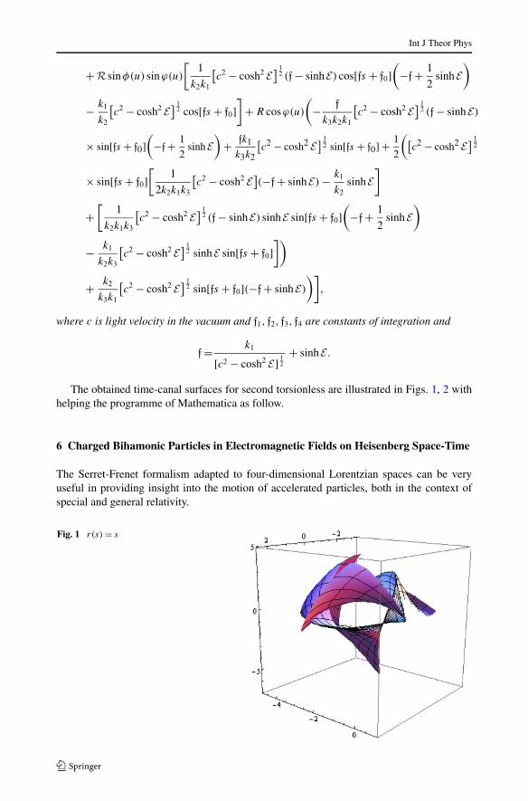
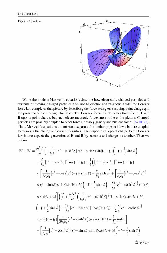
The obtained time-canal surfaces for second torsionless are illustrated in Figs. 1, 2 withhelping the programme of Mathematica as follow.

6 Charged Bihamonic Particles in Electromagnetic Fields on Heisenberg Space-Time

The Serret-Frenet formalism adapted to four-dimensional Lorentzian spaces can be veryuseful in providing insight into the motion of accelerated particles, both in the context ofspecial and general relativity.

Fig. 1 r(s) = s

Int J Theor Phys

Fig. 2 r(s) = tan s

While the modern Maxwell’s equations describe how electrically charged particles andcurrents or moving charged particles give rise to electric and magnetic fields, the Lorentzforce law completes that picture by describing the force acting on a moving point charge q inthe presence of electromagnetic fields. The Lorentz force law describes the effect of E andB upon a point charge, but such electromagnetic forces are not the entire picture. Chargedparticles are possibly coupled to other forces, notably gravity and nuclear forces [8–10, 26].Thus, Maxwell’s equations do not stand separate from other physical laws, but are coupledto them via the charge and current densities. The response of a point charge to the Lorentzlaw is one aspect; the generation of E and B by currents and charges is another. Then weobtain

B2 − E2 = m2c4

e2

(− f

k2k1

[c2 − cosh2 E

] 12 (f− sinhE) sin[fs + f0]

(−f+ 1

2sinhE

)

+ fk1

k2

[c2 − cosh2 E

] 12 sin[fs + f0] + 1

2

([c2 − cosh2 E

] 12 sin[fs + f0]

×[

1

2k2k1

[c2 − cosh2 E

](−f+ sinhE) − k1

k2sinhE

]+

[1

k2k1

[c2 − cosh2 E

] 12

× (f− sinhE) sinhE sin[fs + f0](

−f+ 1

2sinhE

)− k1

k2

[c2 − cosh2 E

] 12 sinhE

× sin[fs + f0]]))2

+ m2c4

e2

(f

k2k1

[c2 − cosh2 E

] 12 (f− sinhE) cos[fs + f0]

(−f+ 1

2sinhE

)− fk1

k2

[c2 − cosh2 E

] 12 cos[fs + f0] − 1

2

([c2 − cosh2 E

] 12

× cos[fs + f0][

1

2k2k1

[c2 − cosh2 E

](−f+ sinhE) − k1

k2sinhE

]

+[

1

k2k1

[c2 − cosh2 E

] 12 (f− sinhE) sinhE cos[fs + f0]

(−f+ 1

2sinhE

)

Int J Theor Phys

− k1

k2

[c2 − cosh2 E

] 12 sinhE cos[fs + f0]

]))2

+ 1

2

m2c4

e2

([1

k2k1

[c2 − cosh2 E

](f− sinhE) sin 2[fs + f0]

(−f+ 1

2sinhE

)

− k1

k2

[c2 − cosh2 E

]sin 2[fs + f0]

])2

+ m2c4

e2

[c2 − cosh2 E

](f− sinhE)2,

where c is light velocity in the vacuum and f1, f2, f3, f4 are constants of integration.

7 Conlusion

Biharmonic functions are utilized in many physical situations, particularly in fluid dynamicsand elasticity problems. Most important applications of the theory of functions of a complexvariable were obtained in the plane theory of elasticity and in the approximate theory ofplates subject to normal loading.

On the other hand, the electromagnetic field tensor, expressed by a four-by-four matrix,is used to describe the electromagnetic field intensity. This tensor provides a convenient ex-pression for the Lorentz force and therefore can describe the evolution of a charged particle.

In this paper, we introduce a new space-time using Heisenberg group and call thisspace as “Heisenberg space-time”. We give a geometrical description of time-canal surfacesaround timelike biharmonic particle in Heisenberg space-time H4

1. Moreover, we obtainLorentz transformations this particles.

Acknowledgements The authors would like to express their sincere gratitude to the referees for the valu-able suggestions to improve the paper.

References

1. Bossavit, A.: Differential forms and the computation of fields and forces in electromagnetism. Eur. J.Mech. B, Fluids 10, 474–488 (1991)

2. Caltenco, J.H., Linares, R., López-Bonilla, J.L.: Intrinsic geometry of curves and the Lorentz equation.Czechoslov. J. Phys. 52, 839–842 (2002)

3. Capovilla, R., Chryssomalakos, C., Guven, J.: Hamiltonians for curves. J. Phys. A, Math. Gen. 35, 6571–6587 (2002)

4. Carmeli, M.: Motion of a charge in a gravitational field. Phys. Rev. B 138, 1003–1007 (1965)5. Deschamps, G.A.: Exterior Differential Forms. Springer, Berlin (1970)6. Gray, A.: Modern Differential Geometry of Curves and Surfaces with Mathematica. CRC Press, Boca

Raton (1998)7. Eells, J., Lemaire, L.: A report on harmonic maps. Bull. Lond. Math. Soc. 10, 1–68 (1978)8. Einstein, A.: Relativity: The Special and General Theory. Henry Holt, New York (1920)9. Hehl, F.W., Obhukov, Y.: Foundations of Classical Electrodynamics. Birkhauser, Basel (2003)

10. Honig, E., Schucking, E., Vishveshwara, C.: Motion of charged particles in homogeneous electromag-netic fields. J. Math. Phys. 15, 774–781 (1974)

11. Jiang, G.Y.: 2-harmonic maps and their first and second variational formulas. Chin. Ann. Math., Ser. A7(4), 389–402 (1986)

12. Körpınar, T., Turhan, E.: On characterization of B-canal surfaces in terms of biharmonic B-slant helicesaccording to Bishop frame in Heisenberg group Heis3. J. Math. Anal. Appl. 382, 57–65 (2012)

13. Körpınar, T., Turhan, E., Asil, V.: Tangent Bishop spherical images of a biharmonic B-slant helix in theHeisenberg group Heis3. Iranian. J. Sci. Technol. Trans. A, Sci. 35, 265–271 (2012)

14. Körpınar, T., Turhan, E.: Tubular Surfaces Around Timelike Biharmonic Curves in Lorentzian Heisen-berg Group Heis3. Anal. Stiintifice Univ. Ovidius Const., Ser. Mat. 20(1), 431–445 (2012)

Int J Theor Phys

15. Körpınar, T., Turhan, E.: Time-tangent surfaces around biharmonic particles and its Lorentz transforma-tions in Heisenberg space-time. Int. J. Theor. Phys. 52, 4427–4438 (2013)

16. Möller, C.: In: The Theory of Relativity. Clarendon Oxford (1952)17. O’Neill, B.: Semi-Riemannian Geometry. Academic Press, New York (1983)18. Pina, E.: Lorentz transformation and the motion of a charge in a constant electromagnetic field. Rev.

Mex. Fis. 16, 233–236 (1967)19. Ringermacher, H.: Intrinsic geometry of curves and the Minkowski force. Phys. Lett. A 74, 381–383

(1979)20. Synge, J.L.: Relativity: The General Theory. North Holland, Amsterdam (1960)21. Synge, J.L.: Time-like helices in flat space-time. Proc. R. Ir. Acad., Sect. A 65, 27–41 (1967)22. Trocheris, M.G.: Electrodynamics in a rotating frame of reference. Philos. Mag. 7, 1143–1155 (1949)23. Turhan, E., Körpınar, T.: On characterization of timelike horizontal biharmonic curves in the Lorentzian

Heisenberg Group Heis3. Z. Naturforsch. A 65a, 641–648 (2010)24. Turhan, E., Körpınar, T.: Position vector of spacelike biharmonic curves in the Lorentzian Heisenberg

group Heis3. Anal. Stiintifice Univ. Ovidius Const., Ser. Mat. 19, 285–296 (2011)25. Turhan, E., Körpınar, T.: On characterization canal surfaces around timelike horizontal biharmonic

curves in Lorentzian Heisenberg group Heis3. Z. Naturforsch. A 66a, 441–449 (2011)26. Weber, J.: Relativity and Gravitation. Interscience, New York (1961)