Embed Size (px)
Citation preview
Machine learning: lecture 16
Tommi S. Jaakkola
MIT AI Lab
Topics
• Structured probability models
– Markov models
– Hidden markov models
Tommi Jaakkola, MIT AI Lab 2
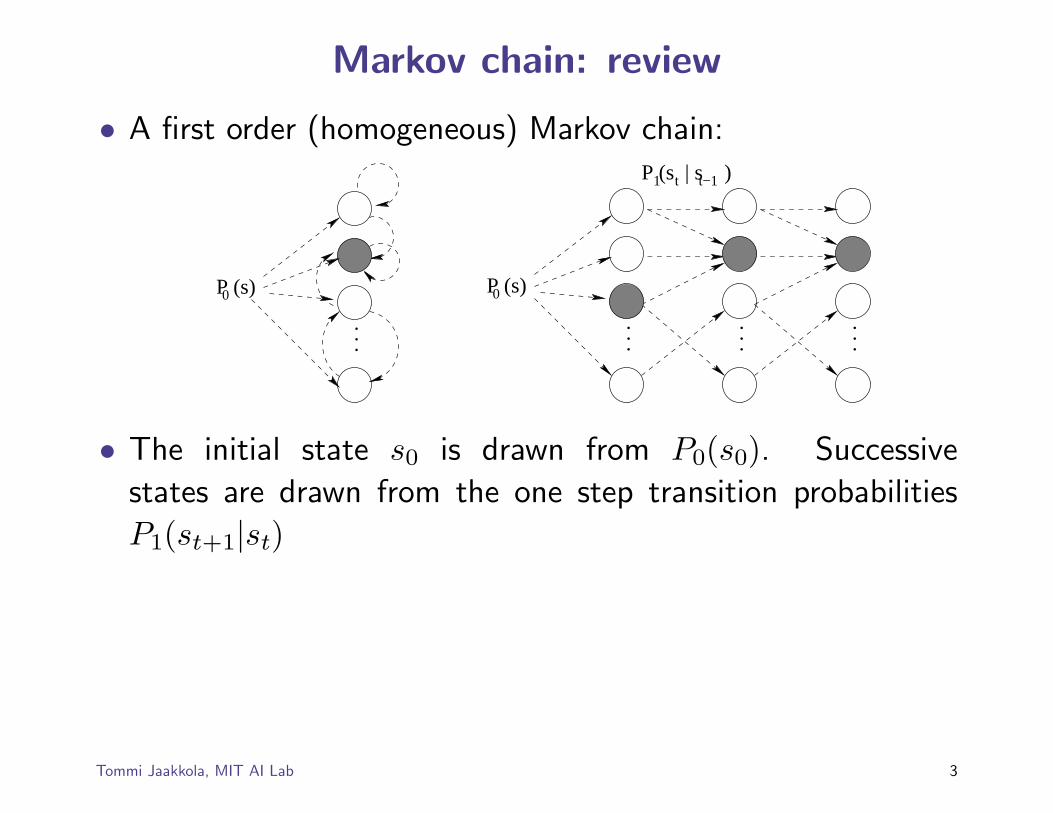
Markov chain: review
• A first order (homogeneous) Markov chain:
P (s)0
. . .
tP (s | s ) t−1
P (s)0
. . .
. . .
. . .
1
• The initial state s0 is drawn from P0(s0). Successive
states are drawn from the one step transition probabilities
P1(st+1|st)
Tommi Jaakkola, MIT AI Lab 3
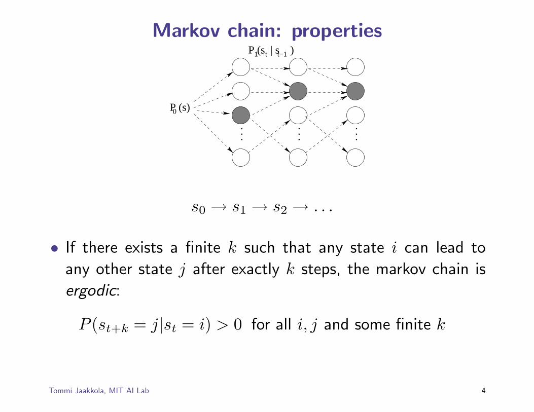
Markov chain: properties tP (s | s ) t−1
P (s)0
. . .
. . .
. . .
1
s0 → s1 → s2 → . . .
• If there exists a finite k such that any state i can lead to
any other state j after exactly k steps, the markov chain is
ergodic:
P (st+k = j|st = i) > 0 for all i, j and some finite k
Tommi Jaakkola, MIT AI Lab 4
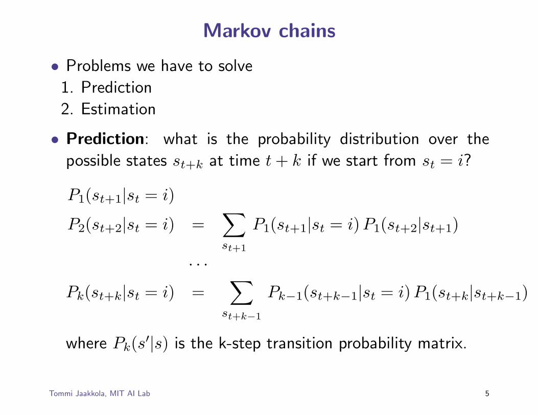
Markov chains
• Problems we have to solve
1. Prediction
2. Estimation
• Prediction: what is the probability distribution over the
possible states st+k at time t + k if we start from st = i?
P1(st+1|st = i)
P2(st+2|st = i) =∑st+1
P1(st+1|st = i) P1(st+2|st+1)
· · ·Pk(st+k|st = i) =
∑st+k−1
Pk−1(st+k−1|st = i) P1(st+k|st+k−1)
where Pk(s′|s) is the k-step transition probability matrix.
Tommi Jaakkola, MIT AI Lab 5
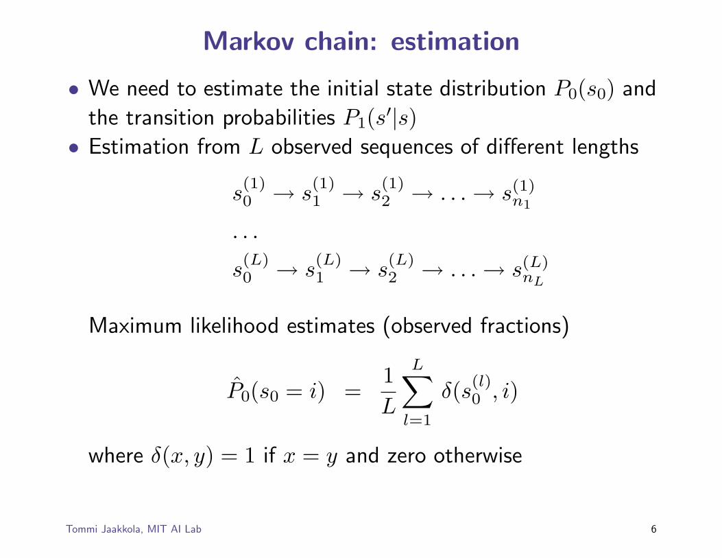
Markov chain: estimation
• We need to estimate the initial state distribution P0(s0) and
the transition probabilities P1(s′|s)• Estimation from L observed sequences of different lengths
s(1)0 → s
(1)1 → s
(1)2 → . . . → s(1)
n1
. . .
s(L)0 → s
(L)1 → s
(L)2 → . . . → s(L)
nL
Maximum likelihood estimates (observed fractions)
P̂0(s0 = i) =1L
L∑l=1
δ(s(l)0 , i)
where δ(x, y) = 1 if x = y and zero otherwise
Tommi Jaakkola, MIT AI Lab 6
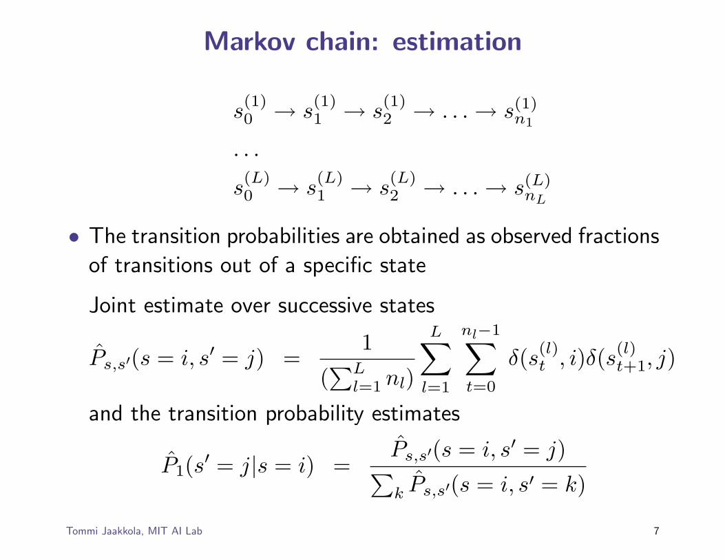
Markov chain: estimation
s(1)0 → s
(1)1 → s
(1)2 → . . . → s(1)
n1
. . .
s(L)0 → s
(L)1 → s
(L)2 → . . . → s(L)
nL
• The transition probabilities are obtained as observed fractions
of transitions out of a specific state
Joint estimate over successive states
P̂s,s′(s = i, s′ = j) =1
(∑L
l=1 nl)
L∑l=1
nl−1∑t=0
δ(s(l)t , i)δ(s(l)
t+1, j)
and the transition probability estimates
P̂1(s′ = j|s = i) =P̂s,s′(s = i, s′ = j)∑k P̂s,s′(s = i, s′ = k)
Tommi Jaakkola, MIT AI Lab 7
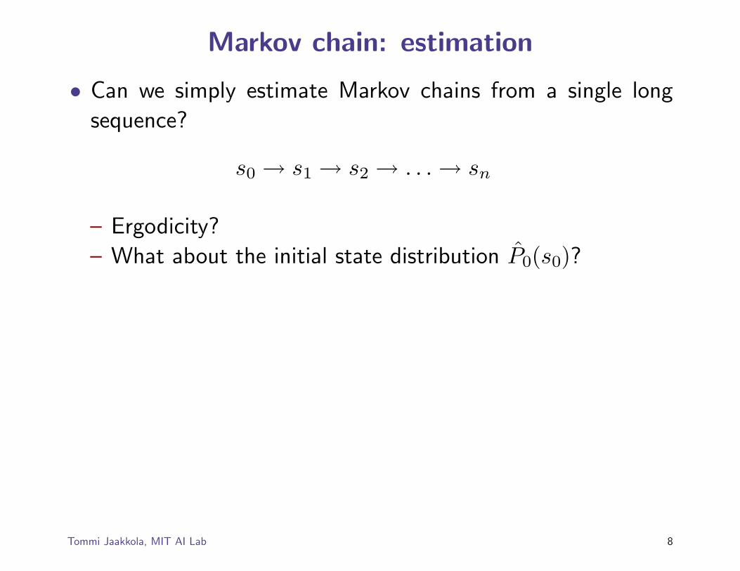
Markov chain: estimation
• Can we simply estimate Markov chains from a single long
sequence?
s0 → s1 → s2 → . . . → sn
– Ergodicity?
– What about the initial state distribution P̂0(s0)?
Tommi Jaakkola, MIT AI Lab 8
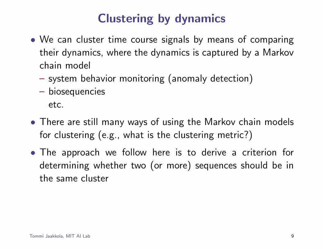
Clustering by dynamics
• We can cluster time course signals by means of comparing
their dynamics, where the dynamics is captured by a Markov
chain model
– system behavior monitoring (anomaly detection)
– biosequencies
etc.
• There are still many ways of using the Markov chain models
for clustering (e.g., what is the clustering metric?)
• The approach we follow here is to derive a criterion for
determining whether two (or more) sequences should be in
the same cluster
Tommi Jaakkola, MIT AI Lab 9
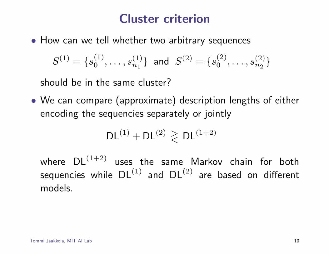
Cluster criterion
• How can we tell whether two arbitrary sequences
S(1) = {s(1)0 , . . . , s(1)
n1} and S(2) = {s(2)
0 , . . . , s(2)n2}
should be in the same cluster?
• We can compare (approximate) description lengths of either
encoding the sequencies separately or jointly
DL(1) + DL(2) >< DL(1+2)
where DL(1+2) uses the same Markov chain for both
sequencies while DL(1) and DL(2) are based on different
models.
Tommi Jaakkola, MIT AI Lab 10
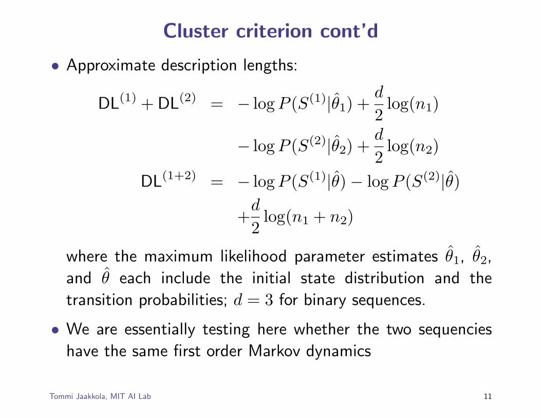
Cluster criterion cont’d
• Approximate description lengths:
DL(1) + DL(2) = − log P (S(1)|θ̂1) +d
2log(n1)
− log P (S(2)|θ̂2) +d
2log(n2)
DL(1+2) = − log P (S(1)|θ̂) − log P (S(2)|θ̂)
+d
2log(n1 + n2)
where the maximum likelihood parameter estimates θ̂1, θ̂2,
and θ̂ each include the initial state distribution and the
transition probabilities; d = 3 for binary sequences.
• We are essentially testing here whether the two sequencies
have the same first order Markov dynamics
Tommi Jaakkola, MIT AI Lab 11
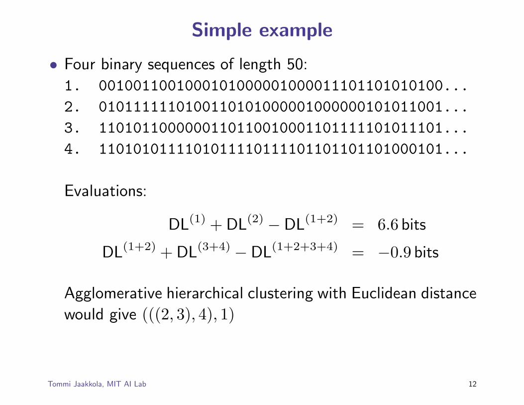
Simple example
• Four binary sequences of length 50:
1. 0010011001000101000001000011101101010100...2. 0101111110100110101000001000000101011001...3. 1101011000000110110010001101111101011101...4. 1101010111101011110111101101101101000101...
Evaluations:
DL(1) + DL(2) − DL(1+2) = 6.6 bits
DL(1+2) + DL(3+4) − DL(1+2+3+4) = −0.9 bits
Agglomerative hierarchical clustering with Euclidean distance
would give (((2, 3), 4), 1)
Tommi Jaakkola, MIT AI Lab 12
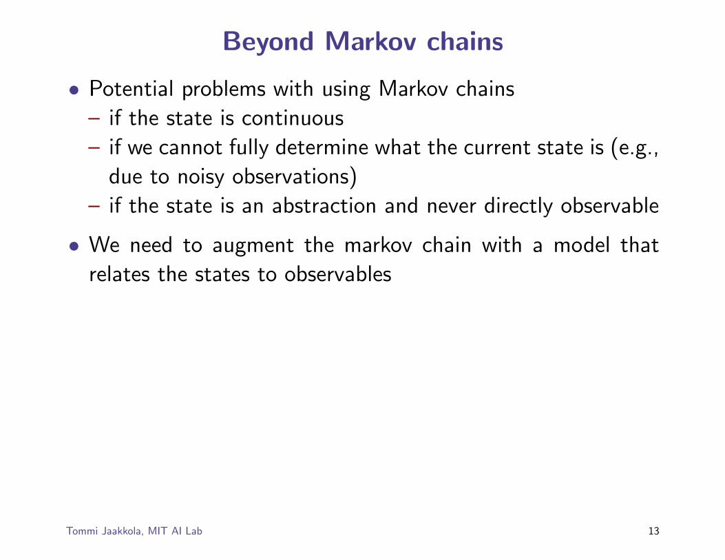
Beyond Markov chains
• Potential problems with using Markov chains
– if the state is continuous
– if we cannot fully determine what the current state is (e.g.,
due to noisy observations)
– if the state is an abstraction and never directly observable
• We need to augment the markov chain with a model that
relates the states to observables
Tommi Jaakkola, MIT AI Lab 13
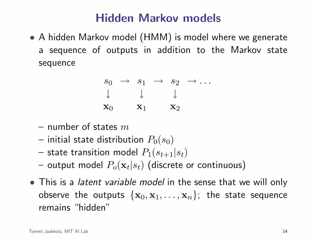
Hidden Markov models
• A hidden Markov model (HMM) is model where we generate
a sequence of outputs in addition to the Markov state
sequence
s0
↓x0
→ s1
↓x1
→ s2
↓x2
→ . . .
– number of states m
– initial state distribution P0(s0)– state transition model P1(st+1|st)– output model Po(xt|st) (discrete or continuous)
• This is a latent variable model in the sense that we will only
observe the outputs {x0,x1, . . . ,xn}; the state sequence
remains “hidden”
Tommi Jaakkola, MIT AI Lab 14
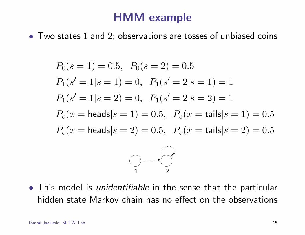
HMM example
• Two states 1 and 2; observations are tosses of unbiased coins
P0(s = 1) = 0.5, P0(s = 2) = 0.5
P1(s′ = 1|s = 1) = 0, P1(s′ = 2|s = 1) = 1
P1(s′ = 1|s = 2) = 0, P1(s′ = 2|s = 2) = 1
Po(x = heads|s = 1) = 0.5, Po(x = tails|s = 1) = 0.5
Po(x = heads|s = 2) = 0.5, Po(x = tails|s = 2) = 0.5
1 2
• This model is unidentifiable in the sense that the particular
hidden state Markov chain has no effect on the observations
Tommi Jaakkola, MIT AI Lab 15
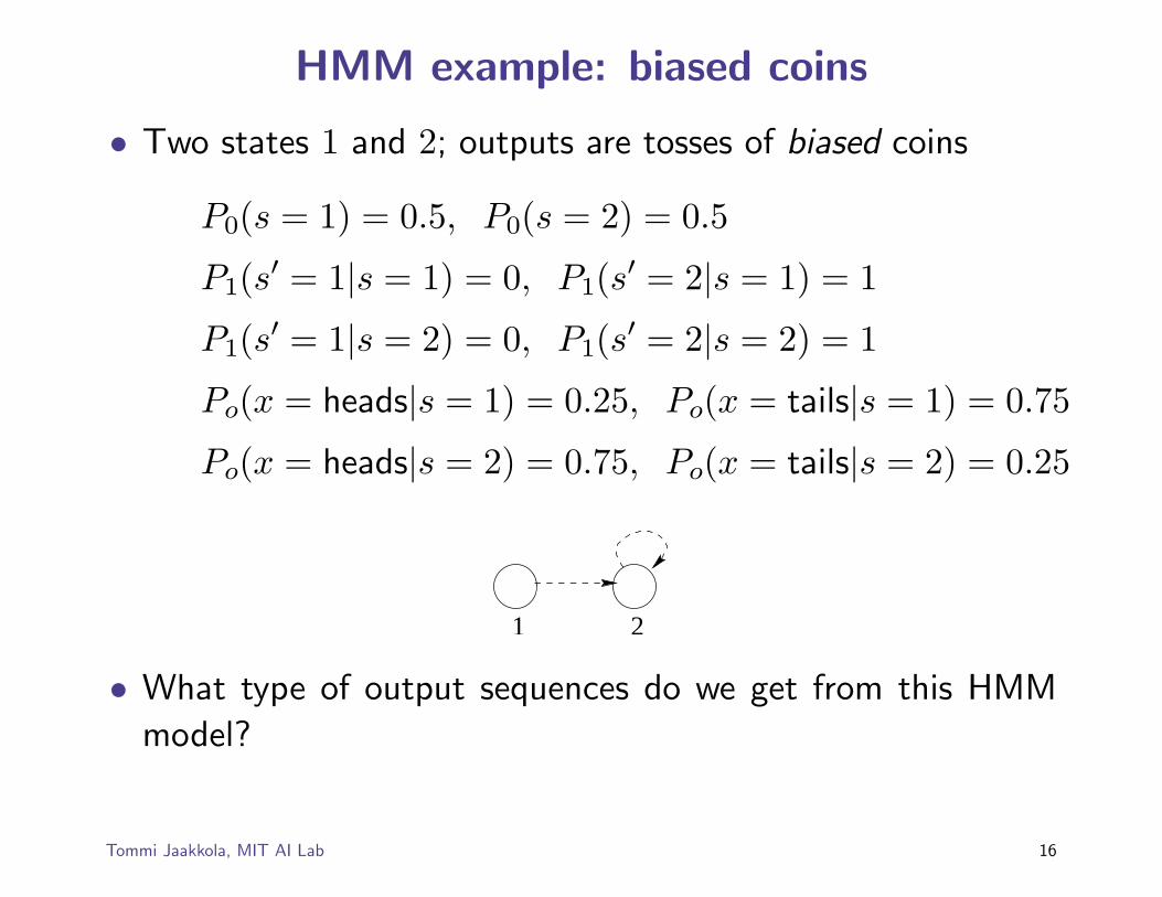
HMM example: biased coins
• Two states 1 and 2; outputs are tosses of biased coins
P0(s = 1) = 0.5, P0(s = 2) = 0.5
P1(s′ = 1|s = 1) = 0, P1(s′ = 2|s = 1) = 1
P1(s′ = 1|s = 2) = 0, P1(s′ = 2|s = 2) = 1
Po(x = heads|s = 1) = 0.25, Po(x = tails|s = 1) = 0.75
Po(x = heads|s = 2) = 0.75, Po(x = tails|s = 2) = 0.25
1 2
• What type of output sequences do we get from this HMM
model?
Tommi Jaakkola, MIT AI Lab 16
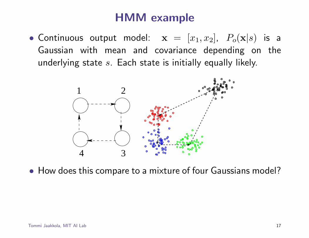
HMM example
• Continuous output model: x = [x1, x2], Po(x|s) is a
Gaussian with mean and covariance depending on the
underlying state s. Each state is initially equally likely.
1 2
34
• How does this compare to a mixture of four Gaussians model?
Tommi Jaakkola, MIT AI Lab 17
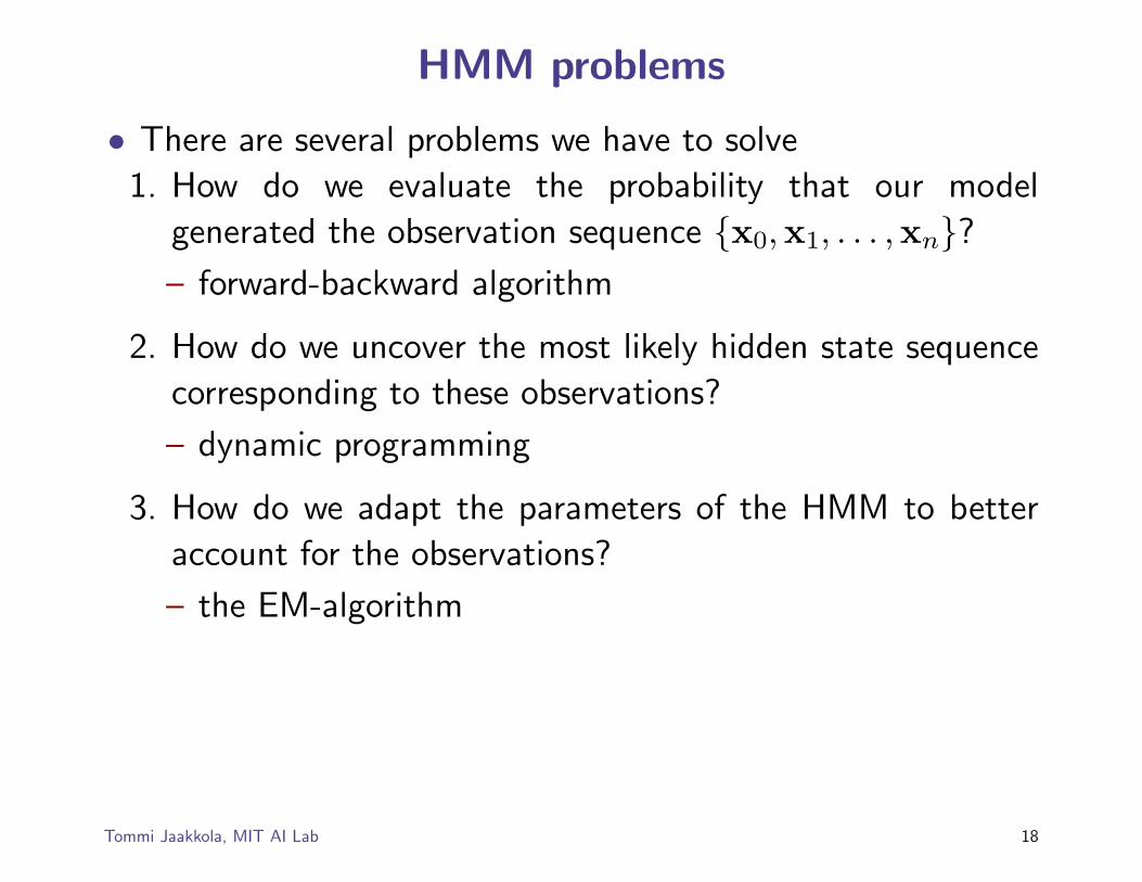
HMM problems
• There are several problems we have to solve
1. How do we evaluate the probability that our model
generated the observation sequence {x0,x1, . . . ,xn}?– forward-backward algorithm
2. How do we uncover the most likely hidden state sequence
corresponding to these observations?
– dynamic programming
3. How do we adapt the parameters of the HMM to better
account for the observations?
– the EM-algorithm
Tommi Jaakkola, MIT AI Lab 18
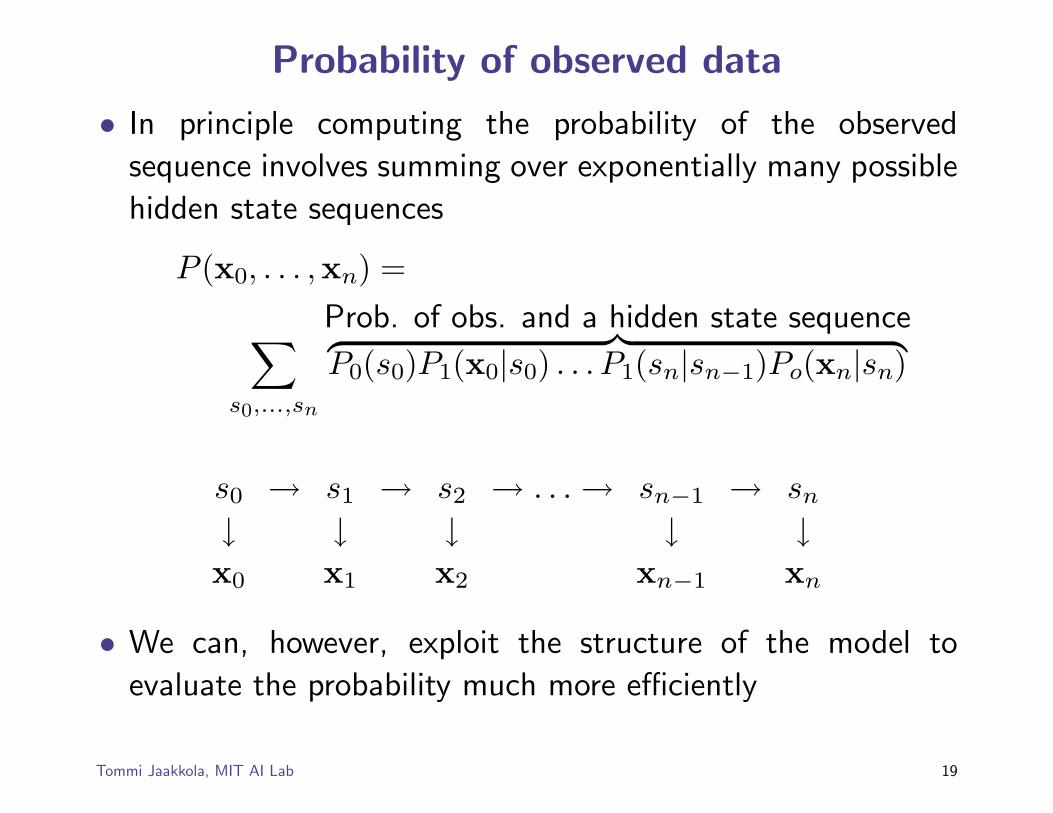
Probability of observed data
• In principle computing the probability of the observed
sequence involves summing over exponentially many possible
hidden state sequences
P (x0, . . . ,xn) =
∑s0,...,sn
Prob. of obs. and a hidden state sequence︷ ︸︸ ︷P0(s0)P1(x0|s0) . . . P1(sn|sn−1)Po(xn|sn)
s0
↓x0
→ s1
↓x1
→ s2
↓x2
→ . . . → sn−1
↓xn−1
→ sn
↓xn
• We can, however, exploit the structure of the model to
evaluate the probability much more efficiently
Tommi Jaakkola, MIT AI Lab 19
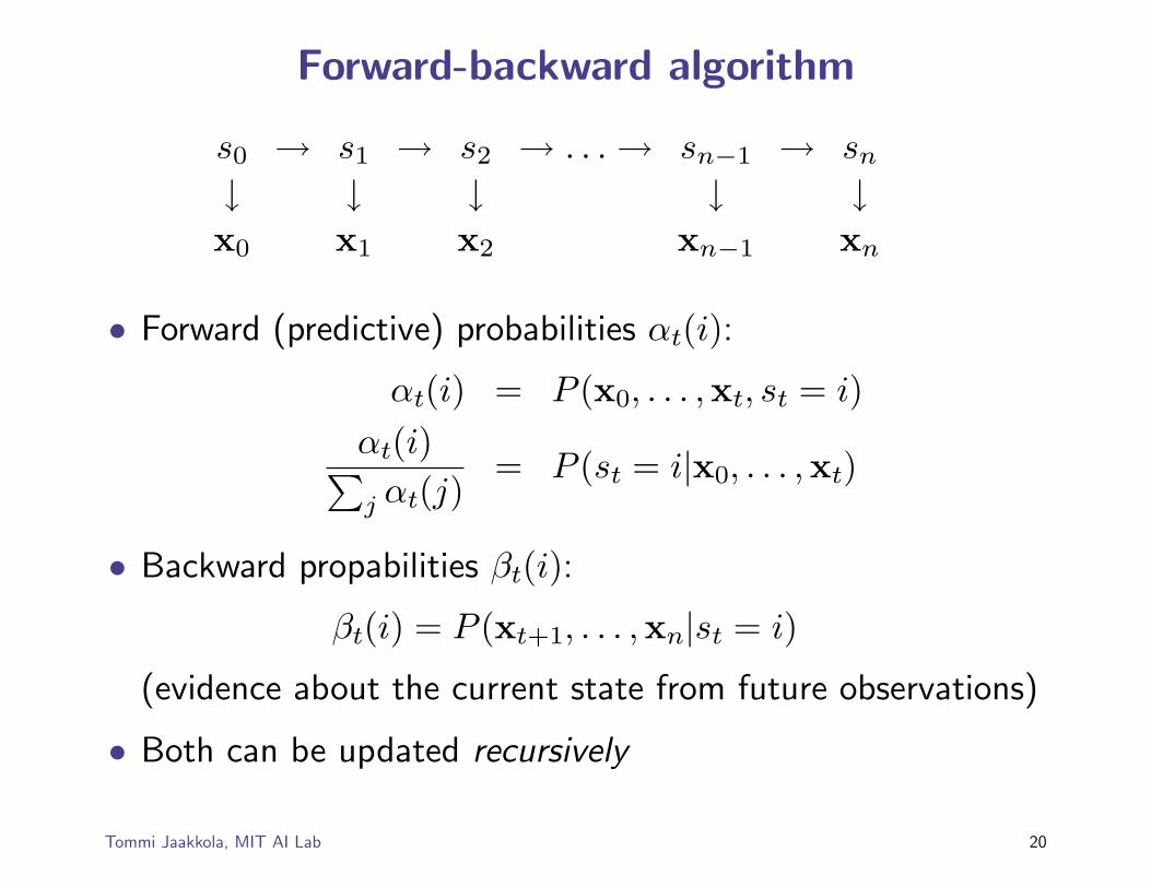
Forward-backward algorithm
s0
↓x0
→ s1
↓x1
→ s2
↓x2
→ . . . → sn−1
↓xn−1
→ sn
↓xn
• Forward (predictive) probabilities αt(i):
αt(i) = P (x0, . . . ,xt, st = i)αt(i)∑j αt(j)
= P (st = i|x0, . . . ,xt)
• Backward propabilities βt(i):
βt(i) = P (xt+1, . . . ,xn|st = i)
(evidence about the current state from future observations)
• Both can be updated recursively
Tommi Jaakkola, MIT AI Lab 20
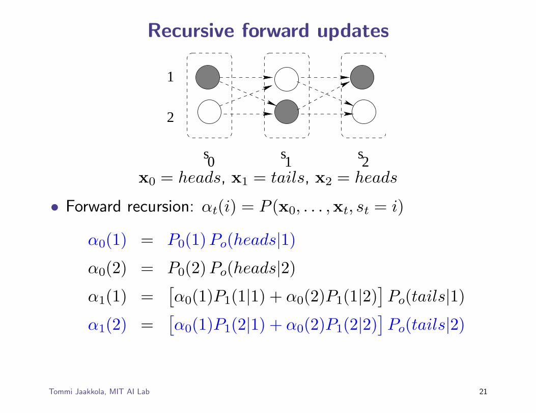
Recursive forward updates
s0 s2s1
1
2
x0 = heads, x1 = tails, x2 = heads
• Forward recursion: αt(i) = P (x0, . . . ,xt, st = i)
α0(1) = P0(1)Po(heads|1)
α0(2) = P0(2)Po(heads|2)
α1(1) =[α0(1)P1(1|1) + α0(2)P1(1|2)
]Po(tails|1)
α1(2) =[α0(1)P1(2|1) + α0(2)P1(2|2)
]Po(tails|2)
Tommi Jaakkola, MIT AI Lab 21
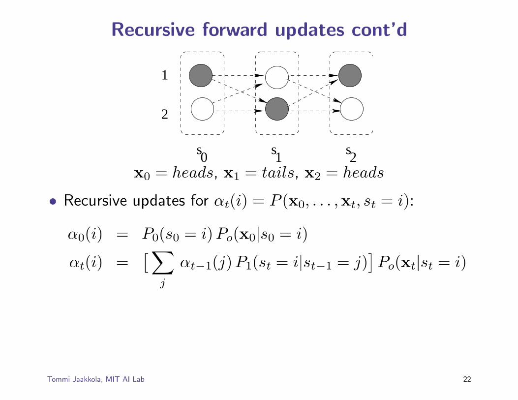
Recursive forward updates cont’d
s0 s2s1
1
2
x0 = heads, x1 = tails, x2 = heads
• Recursive updates for αt(i) = P (x0, . . . ,xt, st = i):
α0(i) = P0(s0 = i) Po(x0|s0 = i)
αt(i) =[∑
j
αt−1(j) P1(st = i|st−1 = j)]Po(xt|st = i)
Tommi Jaakkola, MIT AI Lab 22
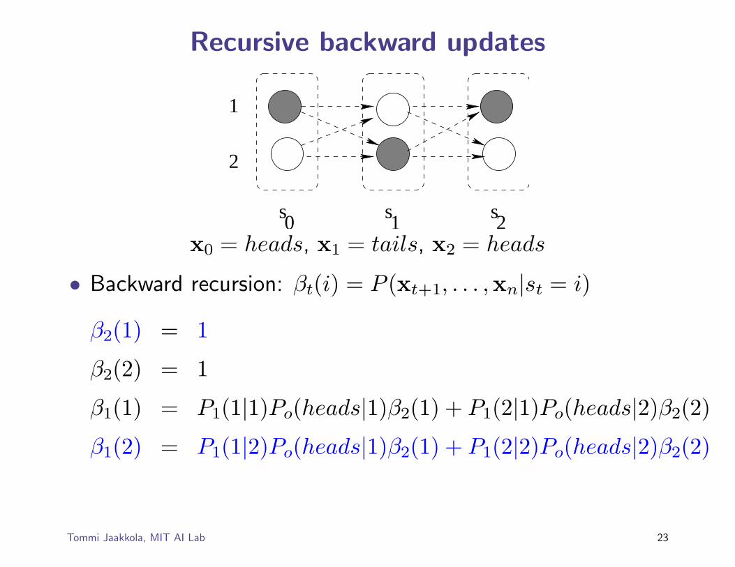
Recursive backward updates
s0 s2s1
1
2
x0 = heads, x1 = tails, x2 = heads
• Backward recursion: βt(i) = P (xt+1, . . . ,xn|st = i)
β2(1) = 1
β2(2) = 1
β1(1) = P1(1|1)Po(heads|1)β2(1) + P1(2|1)Po(heads|2)β2(2)
β1(2) = P1(1|2)Po(heads|1)β2(1) + P1(2|2)Po(heads|2)β2(2)
Tommi Jaakkola, MIT AI Lab 23
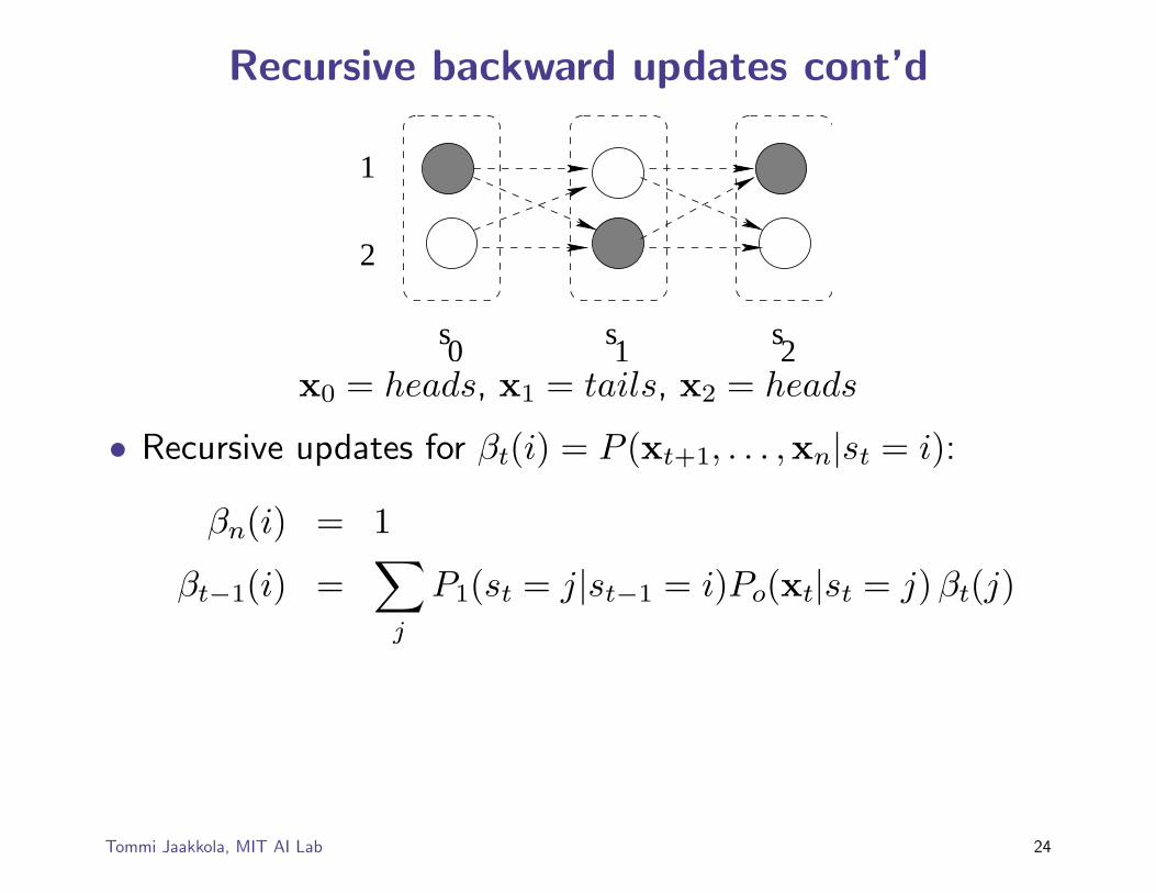
Recursive backward updates cont’d
s0 s2s1
1
2
x0 = heads, x1 = tails, x2 = heads
• Recursive updates for βt(i) = P (xt+1, . . . ,xn|st = i):
βn(i) = 1
βt−1(i) =∑
j
P1(st = j|st−1 = i)Po(xt|st = j) βt(j)
Tommi Jaakkola, MIT AI Lab 24