Embed Size (px)
Citation preview
DOI: 10.1007/s004530010002
Algorithmica (2000) 27: 5–20 Algorithmica© 2000 Springer-Verlag New York Inc.
Topology-Oriented Implementation—An Approach toRobust Geometric Algorithms
K. Sugihara,1 M. Iri, 2 H. Inagaki,3 and T. Imai4
Abstract. This paper presents an approach, called the “topology-oriented approach,” to numerically robustgeometric algorithms. In this approach, the basic part of the algorithm is described in terms of combinatorialand topological computation primarily; this description guarantees robustness of the algorithm because com-binatorial and topological computation is never contaminated with numerical errors. However, this part of thealgorithm is usually nondeterministic, the flow of processing containing many alternative branches. Hence,numerical computation is used in order to choose the branch that seems the most promising to lead to thecorrect answer. The algorithm designed in this way is robust and simple. The basic idea of this approach aswell as the basic properties of the resulting algorithms is shown with examples.
Key Words. Clipping a convex polyhedron, Line-segment Voronoi diagram, Robust implementation, Topo-logical consistency.
1. Introduction. There is a great gap betweentheoretically correctgeometric algo-rithms andpractically valid computer programs. This is mainly because actual com-putation contains numerical errors; these errors sometimes generate inconsistencies intopology and thus make computer programs fail.
To overcome this difficulty many approaches have been proposed. Roughly speaking,they can be classified into three categories according to how much they rely on thenumerical computation.
The approaches in the first category rely on the numerical computation “moderately.”They use inexact arithmetic, such as floating-point arithmetic, but they assume that theamount of error in the computation is bounded. On the basis of evaluation of the errors, thepredicates computed in the algorithm are divided into reliable and unreliable. The reliablepredicates are used positively while the unreliable ones are used carefully in order to avoidinconsistency. This category includes the hidden-variable approach [25], theε-geometryapproach [11], the approximate predicate approach [7], [8], the tolerance approach [33],[45], and other error-analysis approaches [5], [14], [15], [30]. In these approaches, in-dividual problems more or less require their own sophistications, but once they are im-plemented, they run fast because the floating-point arithmetic can be executed quickly.
1 Department of Mathematical Engineering and Information Physics, Graduate School of Engineering, Uni-versity of Tokyo, 7-3-1 Hongo, Bunkyo-ku, Tokyo 113-8656, Japan.2 Department of Information and System Engineering, Faculty of Science and Engineering, Chuo University,1-13-27 Kasuga, Bunkyo-ku, Tokyo 112-8551, Japan.3 Department of Information and Computer Engineering, Toyota National College of Technology, 2-1 Eisei-cho, Toyota-shi, Aichi 471-8525, Japan.4 Department of Design and Information Sciences, Wakayama University, 930 Sakaedani, Wakayama 640-8510, Japan.
Received December 12, 1996; revised June 1, 1998. Communicated by S. Fortune.
6 K. Sugihara, M. Iri, H. Inagaki, and T. Imai
The approaches in the second category rely on the numerical computation “com-pletely.” They use exact arithmetic such as integer arithmetic and thus always obtain cor-rect predicates. In the early days their primal interest was how to achieve exact arithmetic[10], [28], [40], [44], and how to cope with degeneracy [6], [43]. It is now considered astandard method to use multiple-precision arithmetic together with symbolic perturba-tion. This method seems promising because theoretical algorithms can be implementeddirectly. The main practical issue is how to decrease the cost of exact computation.
A typical technique is the floating-point filter, in which the predicates are first com-puted in floating-point arithmetic, and only when it turns out to be unreliable is exactarithmetic used [1], [9], [21], [38]. A more sophisticated version is an adaptive filterin which the precision of the filter is adjusted [31]. Methods to decrease the requiredprecision are also proposed. They include the basis-reduction technique [3], [4], themodular arithmetic techniques [2], [17], and the implicit representation technique [23].Because of these acceleration techniques, many geometric algorithms concerned withlow-degree objects such as lines and planes can be implemented into practically fastsoftware [24].
The approaches in the third category rely on numerical values the least. In other words,they aim at algorithms that are robust even if numerical errors are large. This categoryincludes the axiomatic approach [22], [29], in which numerical computation is done onlywhen it is not redundant; this approach is also called the parsimonious approach.
In this paper we present another approach to robustness belonging to the third cate-gory, which we call the “topology-oriented approach” or the “combinatorial-abstractionapproach.” In this approach the basic part of an algorithm is described in terms of com-binatorial and topological computation primarily, and numerical computation is used assecondary information. A remarkable point in this approach is that the inconsistencyissue is completely separated from the numerical error issue. We need not consider theamount of numerical errors when we construct the basic part of the robust algorithm; inthis sense the design process is simple.
We proposed the first idea of this approach in 1988 [39]. Since then we have beendeveloping this approach by applying the idea to many geometric problems, such asconstruction of various Voronoi/Delaunay diagrams in two and three dimensions [18]–[20], [27], [35], [41], [42], construction of three-dimensional convex hulls [26], [36],and intersection of convex polyhedra [37].
In what follows, we summarize the basic idea behind these works from a unifyingpoint of view, and thus try to clarify the general idea of the topology-oriented approach.
2. Robustness against Numerical Errors and Consistency in Topology.Let P bea geometric problem, and letf be a theoretical algorithm to solveP. By a “theoretical”algorithm, we mean an algorithm that is designed assuming precise arithmetic, namely,one whose correctness is based on the assumption that no numerical error takes place inthe computation.
The algorithmf can be considered a mapping from the set4(P) of all possible inputsto the setÄ(P) of all possible outputs. Each inputX ∈ 4(P) represents an instance ofthe problemP, and the corresponding outputf (X) ∈ Ä(P) is a solution of the probleminstance.
Topology-Oriented Implementation—An Approach to Robust Geometric Algorithms 7
Both the input and the output can be divided into the “combinatorial and/or topologicalpart” (“topological part” for short) and the “metric part.” We represent the topologicalpart by a subscript T and the metric part by a subscript M. More specifically, the inputX is divided into the topological partXT and the metric partXM, and the outputf (X)is divided into the topological partfT(X) and the metric partfM(X).
For example, suppose thatP is the problem of constructing the Voronoi diagramfor a finite number of given points in the plane. Then the topological partXT of theinput consists of a single integer to represent the numbern of points, and the metricpart XM is the set of then pairs of coordinates of the points:XT = {n} and XM ={x1, y1, . . . , xn, yn}. The topological partfT(X)of the output is the planar graph structureconsisting of the Voronoi vertices and the Voronoi edges, and the metric partfM(X)consists of the coordinates of the Voronoi vertices and the directions of the infiniteVoronoi edges.
For another example, suppose thatP is the problem of constructing the intersectionof two convex polyhedra in three-dimensional space. ThenXT consists of the incidencestructure among the vertices, the edges, and the faces of the two polyhedra, andXM
consists of the three-dimensional coordinates of the vertices and/or the coefficientsof the face equations. Similarly,fT(X) and fM(X) are the topological part and themetric part, respectively, of the polyhedron which is the intersection of the two inputpolyhedra.
Let f denote an actually implemented computer program to solveP. The programf may be a simple translation of the algorithmf into a programming language, or itmay be something more sophisticated aiming at robustness. The programf can also beconsidered a mapping from the input set to the output set. However, in actual situations,the program runs in finite-precision arithmetic, and consequently the behavior off isusually different from that off .
The programf is said to benumerically robust(or robustfor short) if f (X) is definedfor any inputX in 4(P). In other words,f is robust if it defines a total (not partial)function from4(P) to supersetÄ(P) ofÄ(P), i.e., if the program always carries out thetask, ending up with some output, neither entering into an endless loop nor terminatingabnormally.
The program f is said to betopologically consistent(or consistentfor short) iff is robust and fT(X) ∈ ÄT(P) for any X ∈ 4(P). In other words, f is consis-tent if the topological partfT(X) of the output coincides with the topological partfT(X′) of the correct solution of some instanceX′ (not necessarily equal toX) of theproblemP.
Our goal is to constructf that is at least robust and hopefully consistent.
3. Basic Idea. In the topology-oriented approach, we start with the following assump-tions.
ASSUMPTION1. Logical and combinatorial computations can be done correctly, whereasnumerical computations contain errors.
ASSUMPTION2. There is no a priori bound available on the amount of numerical errors.
8 K. Sugihara, M. Iri, H. Inagaki, and T. Imai
The readers might feel that Assumption 2 is too pessimistic, because a certain precisionis usually guaranteed in actual computation. However, we do not like to be pessimistic,but just want to show that, even if we do not rely on numerical results at all, we canstill design robust algorithms. As we show later, Assumption 2 necessarily separates therobustness issue from the error-analysis issue, and thus makes the design of the algorithmsimpler.
Suppose that we are given a geometric problemP together with a conventionalalgorithm f to solveP. We construct a robust implementationf of f in the followingthree steps.
Step I. Collect purely topological properties that should be satisfied by the solutions ofthe problemP and that can be checked efficiently. LetQ be the set of such properties.
By “purely topological properties” we mean those properties that can be representedby only combinatorial and/or topological terms, without referring to numerical values.On the other hand “can be checked efficiently” means that the computational cost forchecking the property is acceptable. For example, suppose that the algorithmf runs inO(n logn) time, andq is a topological property possessed by any solution of the problemP. If it is NP-hard to checkq, we should definitely not putq in Q. In general, whetherwe can putq in Q or not depends on the time allowed in applications.
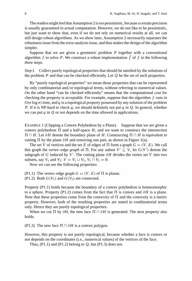
EXAMPLE 1 (Clipping a Convex Polyhedron by a Plane). Suppose that we are given aconvex polyhedron5 and a half-spaceH , and we want to construct the intersection5 ∩ H . Let ∂H denote the boundary plane ofH . Constructing5 ∩ H is equivalent tocutting5 by the plane∂H and removing one part, as shown in Figure 1(a).
The setV of vertices and the setE of edges of5 form a graphG = (V, E). We callthis graph thevertex–edge graphof 5. For any subsetV ′ ⊆ V , let G(V ′) denote thesubgraph ofG induced byV ′. The cutting plane∂H divides the vertex setV into twosubsets, sayV1 andV2: V = V1 ∪ V2, V1 ∩ V2 = ∅.
Now we can see the following properties:
(P1.1) The vertex–edge graphG = (V, E) of 5 is planar.(P1.2) BothG(V1) andG(V2) are connected.
Property (P1.1) holds because the boundary of a convex polyhedron is homeomorphicto a sphere. Property (P1.2) comes from the fact that5 is convex and∂H is a plane.Note that these properties come from the convexity of5 and the convexity is a metricproperty. However, both of the resulting properties are stated in combinatorial termsonly. Hence they are purely topological properties.
When we cut5 by ∂H, the new face5 ∩ ∂H is generated. The next property alsoholds.
(P1.3) The new face5 ∩ ∂H is a convex polygon.
However, this property is not purely topological, because whether a face is convex ornot depends on the coordinates (i.e., numerical values) of the vertices of the face.
Thus, (P1.1) and (P1.2) belong toQ, but (P1.3) does not.
Topology-Oriented Implementation—An Approach to Robust Geometric Algorithms 9
Step II. Describe the basic part of the algorithm only in terms of combinatorial andtopological computation in such a way that the properties inQ are guaranteed. Here weneed not consider degenerate cases.
Combinatorial and topological computations can always be done correctly, and hencewe can design this part of the algorithm without worrying about numerical errors. Wecall this part of the algorithm thetopological skeleton.
Note that numerical computation is not assumed to be exact, and hence we cannotdetect whether the input is degenerate. This is the reason why we ignore degeneratecases. The consequence of this are discussed in Section 5.
The topological skeleton designed in Step II does not specify the behavior of thealgorithm uniquely. It usually contains nondeterministic branches.
EXAMPLE 1 (continued). On the basis of properties (P1.1) and (P1.2), we can constructthe topological skeleton of the algorithm in the following way. The statements in bracketsare comments describing what we actually want to do, and the statements in parenthesesrefer to the example shown in Figure 1.
Fig. 1.Topological skeleton of the intersection operations.
10 K. Sugihara, M. Iri, H. Inagaki, and T. Imai
ALGORITHM 1 (Topological Skeleton for Intersection5 ∩ H ).
Input: Planar graphG = (V, E) [G is supposed to be the vertex–edge graph of5].Output: Planar graphG′ = (V ′, E′) [G′ is hopefully the vertex–edge graph of5 ∩ H ].Procedure:
1. DivideV into V1 andV2 in such a way that (P1.2) is satisfied [hopefully the verticesin V1 are outsideH and those inV2 are insideH ] (in Figure 1(b), the vertices inV1
are represented by solid circles).2. On each edge connectingV1 andV2, generate a new vertex (the vertices represented
by open circles in Figure 1(b)).3. Generate a new circuit passing through all the new vertices and separatingV1 from
V2 (the circuit represented by broken lines in Figure 1(b)).4. Remove the vertices inV1 and the edges incident to them; name the resulting graph
V ′, and report it (the graph in Figure 1(c)).
Note that in this algorithm numerical values are not referred to at all. Steps 2–4 aredeterministic. Only Step 1 is nondeterministic; there are in general many possible waysto divideV into V1 andV2. However, as far as (P1.2) is fulfilled, all the steps can be doneconsistently and the resulting graphG′ is planar.
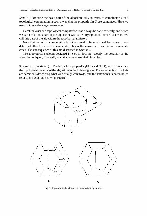
As shown in this example, the topological skeleton usually contains nondeterministicbranches. Hence in general the flow of processing can be represented by a rooted acyclicdirected graph as shown in Figure 2. The algorithm starts at the root node at the top, andgoes downward, choosing one of the branches nondeterministically at each node of thegraph; the algorithm terminates when it reaches one of the leaf nodes. This graph containsthe path reaching the correct solution ofP as shown by the bold path in the figure, but at
Fig. 2.Nondeterministic branches in the topological skeleton of a geometric algorithm.
Topology-Oriented Implementation—An Approach to Robust Geometric Algorithms 11
this moment we do not know which is the correct path because the topological skeletonis described only by combinatorial and topological computations. It should be noted,however, that in this graph any path from the root node represents a consistent behaviorof the algorithm in the sense that the topological properties inQ are preserved at allnodes.
Step III. Conduct numerical computations at each node of the tree in order to choosethe branch that is most likely to lead to the correct solution of the problemP.
Step III adds numerical information to the topological skeleton, and thus makes thebehavior of the algorithm deterministic. We denote the resulting implementation of thealgorithm by f .
EXAMPLE 1 (continued). We use the results of numerical computation in order to makeStep 1 in Algorithm 1 deterministic. More specifically, we add vertexv ∈ V to V1 if thenumerical computation tells us thatv is outsideH and the addition ofv to V1 does notviolate (P1.2).
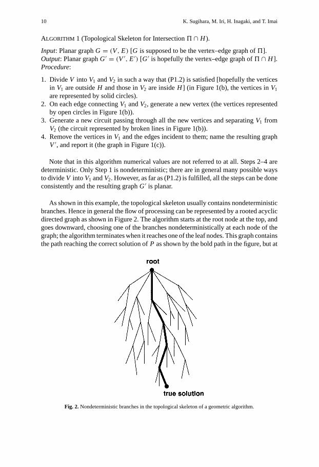
Figure 3 shows an example of the behavior of the computer program constructed inthis way. Figure 3(a) is the output of the program which cuts a large cube by many planestangent to a common paraboloid of revolution (there is no special reason in choosingthis surface; any convex smooth surface can be used similarly). All the floating-pointcomputations were done in single precision. The input is highly degenerated in thesense that many cutting planes have a common point of intersection. Figure 3(b) is thefigure around the degenerate vertex at the top (pointq in Figure 3(a)) magnified by
Fig. 3. Output of Algorithm 1 for degenerate input: (a) output, (b)!diagram around the degenerate vertex atthe top magnified by 5× 10⁵.
12 K. Sugihara, M. Iri, H. Inagaki, and T. Imai
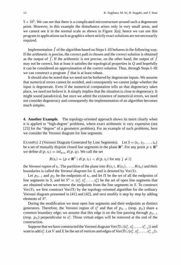
5×10⁵. We can see that there is a complicated microstructure around such a degeneratepoint. However, in this example the disturbance arises only in very small areas, andwe cannot see it in the normal scale as shown in Figure 3(a); hence we can use thisprogram in applications such as graphics where strictly exact solutions are not necessarilyrequired.
Implementationf of the algorithm based on Steps I–III behaves in the following way.If the arithmetic is precise, the correct path is chosen and the correct solution is obtainedas the output off . If the arithmetic is not precise, on the other hand, the output offmay not be correct, but at least it satisfies the topological properties inQ and hopefullyit can be considered an approximation of the correct solution. Thus, through Steps I–IIIwe can construct a programf that is at least robust.
It should also be noted that we need not be bothered by degenerate inputs. We assumethat numerical errors cannot be avoided, and consequently we cannot judge whether theinput is degenerate. Even if the numerical computation tells us that degeneracy takesplace, we need not believe it. It simply implies that the situation isclose todegeneracy. Itmight sound paradoxical, but once we admit the existence of numerical errors, we neednot consider degeneracy and consequently the implementation of an algorithm becomesmuch simpler.
4. Another Example. The topology-oriented approach shows its merit clearly whenit is applied to “high-degree’ problems, where exact arithmetic is very expensive (see[23] for the “degree” of a geometric problem). For an example of such problems, herewe consider the Voronoi diagram for line segments.
EXAMPLE 2 (Voronoi Diagram Generated by Line Segments). LetS= {s1, s2, . . . , sn}be a set of mutually disjoint closed line segments in the planeR2. For any pointp ∈ R2
we defined(p, si ) = infq∈si d(p,q). We call the set
R(si ) = {p ∈ R2 | d(p, si ) < d(p, sj ) for any j 6= i }theVoronoi regionof si . The partition of the plane intoR(s1), R(s2), . . . , R(sn) and theirboundaries is called theVoronoi diagramfor S, and is denoted by Vor(S).
Let p2i−1 and p2i be the endpoints ofsi , and let5 be the set of all the endpoints ofline segments inS, and letSo = {so
1, so2, . . . , s
on} be the set of open line segments that
are obtained when we remove the endpoints from the line segments inS. To constructVor(S), we first construct Vor(5) by the topology-oriented algorithm for the ordinaryVoronoi diagram presented in [41] and [42], and next modify it step by step by addingelements ofSo.
During the modification we treat open line segments and their endpoints as distinctgenerators. Therefore, the Voronoi region ofso
i and that ofp2i−1 (resp. p2i ) share acommon boundary edge; we assume that this edge is on the line passing throughp2i−1
(resp.p2i ) perpendicular tosoi . Those virtual edges will be removed at the end of the
construction.Suppose that we have constructed the Voronoi diagram Vor(5∪{so
1, so2, . . . , s
oi−1})and
want to addsoi . LetV andE be the set of vertices and edges of Vor(5∪{so
1, so2, . . . , s
oi−1}).
Topology-Oriented Implementation—An Approach to Robust Geometric Algorithms 13
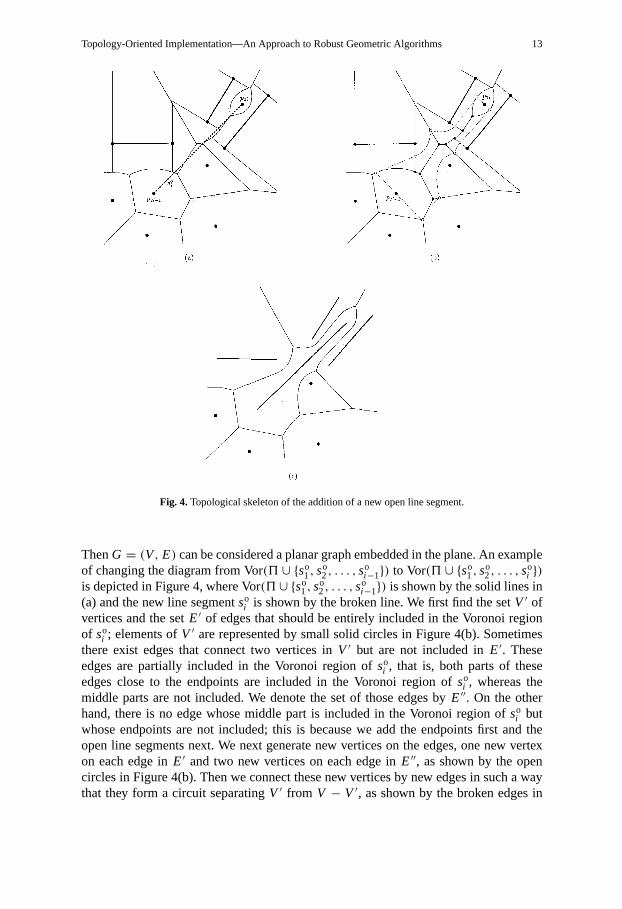
Fig. 4.Topological skeleton of the addition of a new open line segment.
ThenG = (V, E) can be considered a planar graph embedded in the plane. An exampleof changing the diagram from Vor(5 ∪ {so
1, so2, . . . , s
oi−1}) to Vor(5 ∪ {so
1, so2, . . . , s
oi })
is depicted in Figure 4, where Vor(5 ∪ {so1, s
o2, . . . , s
oi−1}) is shown by the solid lines in
(a) and the new line segmentsoi is shown by the broken line. We first find the setV ′ of
vertices and the setE′ of edges that should be entirely included in the Voronoi regionof so
i ; elements ofV ′ are represented by small solid circles in Figure 4(b). Sometimesthere exist edges that connect two vertices inV ′ but are not included inE′. Theseedges are partially included in the Voronoi region ofso
i , that is, both parts of theseedges close to the endpoints are included in the Voronoi region ofso
i , whereas themiddle parts are not included. We denote the set of those edges byE′′. On the otherhand, there is no edge whose middle part is included in the Voronoi region ofso
i butwhose endpoints are not included; this is because we add the endpoints first and theopen line segments next. We next generate new vertices on the edges, one new vertexon each edge inE′ and two new vertices on each edge inE′′, as shown by the opencircles in Figure 4(b). Then we connect these new vertices by new edges in such a waythat they form a circuit separatingV ′ from V − V ′, as shown by the broken edges in
14 K. Sugihara, M. Iri, H. Inagaki, and T. Imai
Figure 4(b). Finally we remove the vertices inV ′ and the edges incident to them asshown in Figure 4(c).
In this process, we can observe the following topological properties:
(P2.1) The subgraph(V ′, E′) is a tree (i.e., a connected graph without circuit).(P2.2) The subgraph(V ′, E′) contains a path connectingR(p2i−1) andR(p2i ).
The graph(V ′, E′) is connected because the Voronoi regionR(si ) is connected, and(V ′, E′) does not contain a circuit because none of the old Voronoi regions disappearsentirely whenso
i is added. Therefore, property (P2.1) holds. Property (P2.2) holds becausethe new line segmentso
i connectsp2i−1 and p2i . On the basis of these observations, wecan construct the topological skeleton of the above process in the following way.
ALGORITHM 2 (Topological Skeleton of the Voronoi Diagram for Line Segments).
Input: Planar graphG = (V, E) [G is supposed to be the graph of Vor(5 ∪ {so1, s
o2,
. . . , soi−1})]
Output: Planar graphG∗ = (V∗, E∗) [hopefully G∗ is the graph of Vor(5 ∪ {so1, s
o2,
. . . , soi })].
Procedure:
1. Select subsetsV ′ ⊆ V and E′ ⊆ E that satisfy (P2.1) and (P2.2) [V ′ and E′ aresupposed to be the set of vertices and that of edges that should be deleted completelyin the addition ofso
i ]. Let E′′ be the edges that connect two vertices inV ′ but are notincluded inE′.
2. Generate a new vertex on each edge inE′ and generate two new vertices on eachedge inE′′.
3. Generate a new circuit passing through all the new vertices and separatingV ′ fromV − V ′.
4. Remove the vertices inV ′ and the edges incident to them. Name the resulting graphG∗ = (V∗, E∗) and report it.
In this algorithm, Step 1 is nondeterministic. We use the result of numerical compu-tation in order to choose asV ′ the set of vertices that are most likely to be deleted in theaddition ofso
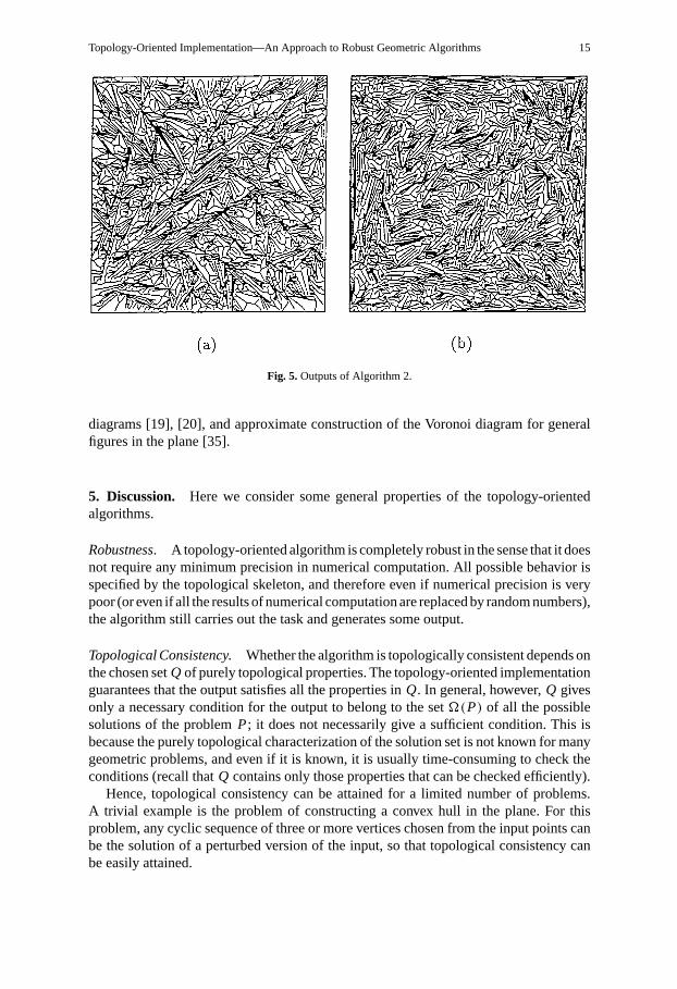
i . Thus, we can make Algorithm 2 deterministic.Figure 5 shows examples of the output of the computer program based on Algorithm 2.
The input set of line segments in Figure 5(a) was obtained in such a way that they weregenerated one by one at random and if they intersect the newer one was cut near thepoint of intersection. On the other hand, the input set of line segments in Figure 5(b)was obtained in such a way that first they were generated at random and next pairs ofmutually intersecting line segments were flipped until no intersection remains.
This method was extended to the construction of the Voronoi diagram for poly-gons [16].
There are many other examples of topology-oriented implementations of geomet-ric algorithms. They include the incremental construction of two-dimensional Voronoidiagrams [41], [42], the divide-and-conquer construction of two-dimensional Voronoidiagrams [27], construction of the three-dimensional convex hull [26], [36], construc-tion of line arrangements in the plane [34], construction of three-dimensional Voronoi
Topology-Oriented Implementation—An Approach to Robust Geometric Algorithms 15
Fig. 5.Outputs of Algorithm 2.
diagrams [19], [20], and approximate construction of the Voronoi diagram for generalfigures in the plane [35].
5. Discussion. Here we consider some general properties of the topology-orientedalgorithms.
Robustness. A topology-oriented algorithm is completely robust in the sense that it doesnot require any minimum precision in numerical computation. All possible behavior isspecified by the topological skeleton, and therefore even if numerical precision is verypoor (or even if all the results of numerical computation are replaced by random numbers),the algorithm still carries out the task and generates some output.
Topological Consistency. Whether the algorithm is topologically consistent depends onthe chosen setQ of purely topological properties. The topology-oriented implementationguarantees that the output satisfies all the properties inQ. In general, however,Q givesonly a necessary condition for the output to belong to the setÄ(P) of all the possiblesolutions of the problemP; it does not necessarily give a sufficient condition. This isbecause the purely topological characterization of the solution set is not known for manygeometric problems, and even if it is known, it is usually time-consuming to check theconditions (recall thatQ contains only those properties that can be checked efficiently).
Hence, topological consistency can be attained for a limited number of problems.A trivial example is the problem of constructing a convex hull in the plane. For thisproblem, any cyclic sequence of three or more vertices chosen from the input points canbe the solution of a perturbed version of the input, so that topological consistency canbe easily attained.
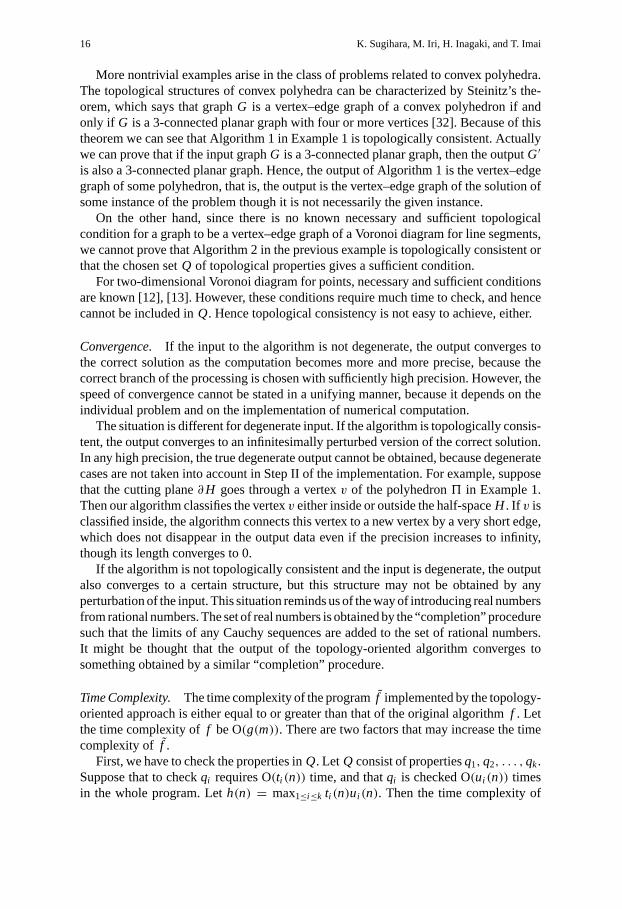
16 K. Sugihara, M. Iri, H. Inagaki, and T. Imai
More nontrivial examples arise in the class of problems related to convex polyhedra.The topological structures of convex polyhedra can be characterized by Steinitz’s the-orem, which says that graphG is a vertex–edge graph of a convex polyhedron if andonly if G is a 3-connected planar graph with four or more vertices [32]. Because of thistheorem we can see that Algorithm 1 in Example 1 is topologically consistent. Actuallywe can prove that if the input graphG is a 3-connected planar graph, then the outputG′
is also a 3-connected planar graph. Hence, the output of Algorithm 1 is the vertex–edgegraph of some polyhedron, that is, the output is the vertex–edge graph of the solution ofsome instance of the problem though it is not necessarily the given instance.
On the other hand, since there is no known necessary and sufficient topologicalcondition for a graph to be a vertex–edge graph of a Voronoi diagram for line segments,we cannot prove that Algorithm 2 in the previous example is topologically consistent orthat the chosen setQ of topological properties gives a sufficient condition.
For two-dimensional Voronoi diagram for points, necessary and sufficient conditionsare known [12], [13]. However, these conditions require much time to check, and hencecannot be included inQ. Hence topological consistency is not easy to achieve, either.
Convergence. If the input to the algorithm is not degenerate, the output converges tothe correct solution as the computation becomes more and more precise, because thecorrect branch of the processing is chosen with sufficiently high precision. However, thespeed of convergence cannot be stated in a unifying manner, because it depends on theindividual problem and on the implementation of numerical computation.
The situation is different for degenerate input. If the algorithm is topologically consis-tent, the output converges to an infinitesimally perturbed version of the correct solution.In any high precision, the true degenerate output cannot be obtained, because degeneratecases are not taken into account in Step II of the implementation. For example, supposethat the cutting plane∂H goes through a vertexv of the polyhedron5 in Example 1.Then our algorithm classifies the vertexv either inside or outside the half-spaceH . If v isclassified inside, the algorithm connects this vertex to a new vertex by a very short edge,which does not disappear in the output data even if the precision increases to infinity,though its length converges to 0.
If the algorithm is not topologically consistent and the input is degenerate, the outputalso converges to a certain structure, but this structure may not be obtained by anyperturbation of the input. This situation reminds us of the way of introducing real numbersfrom rational numbers. The set of real numbers is obtained by the “completion” proceduresuch that the limits of any Cauchy sequences are added to the set of rational numbers.It might be thought that the output of the topology-oriented algorithm converges tosomething obtained by a similar “completion” procedure.
Time Complexity. The time complexity of the programf implemented by the topology-oriented approach is either equal to or greater than that of the original algorithmf . Letthe time complexity off be O(g(m)). There are two factors that may increase the timecomplexity of f .
First, we have to check the properties inQ. Let Q consist of propertiesq1,q2, . . . ,qk.Suppose that to checkqi requires O(ti (n)) time, and thatqi is checked O(ui (n)) timesin the whole program. Leth(n) = max1≤i≤k ti (n)ui (n). Then the time complexity of
Topology-Oriented Implementation—An Approach to Robust Geometric Algorithms 17
the programf is O(g(n) + h(n)). Hence if O(h(n)) is greater than O(g(n)), the timecomplexity increases.
The above argument is much too simplified; actually that is true only whenf behaveslike f . Suppose that the input is far from degenerate and the arithmetic precision ishigh enough to compute all the predicates correctly. Thenf behaves likef , with theadditional cost for checking the properties inQ. Thus the above argument is true.
On the other hand, suppose that the input is relatively close to degenerate (or, equiv-alently, the precision in the arithmetic is relatively low). Thenf may behave quitedifferently from f because numerical errors often generate complicated microstructuressuch as shown in Figure 3(b). In that case, the time complexity of the actual programmay become larger than that of the theoretical algorithm. This is the second factor thatmay increase the time complexity. However, this happens only when the precision istoo poor to get a meaningful output. Usually the programf behaves like the originalalgorithm f with the additional cost of checking the topological properties.
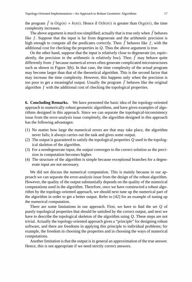
6. Concluding Remarks. We have presented the basic idea of the topology-orientedapproach to numerically robust geometric algorithms, and have given examples of algo-rithms designed in this approach. Since we can separate the topological-inconsistencyissue from the error-analysis issue completely, the algorithm designed in this approachhas the following advantages:
(1) No matter how large the numerical errors are that may take place, the algorithmnever fails; it always carries out the task and gives some output.
(2) The output is guaranteed to satisfy the topological propertiesQ used in the topolog-ical skeleton of the algorithm.
(3) For a nondegenerate input, the output converges to the correct solution as the preci-sion in computation becomes higher.
(4) The structure of the algorithm is simple because exceptional branches for a degen-erate input are not necessary.
We did not discuss the numerical computation. This is mainly because in our ap-proach we can separate the error-analysis issue from the design of the robust algorithm.However, the quality of the output substantially depends on the quality of the numericalcomputations used in the algorithm. Therefore, once we have constructed a robust algo-rithm by the topology-oriented approach, we should next tune up the numerical part ofthe algorithm in order to get a better output. Refer to [42] for an example of tuning upthe numerical computation.
There are some limitations in our approach. First, we have to find the setQ ofpurely topological properties that should be satisfied by the correct output, and next wehave to describe the topological skeleton of the algorithm usingQ. These steps are nottrivial. Actually the topology-oriented approach gives a “principle” for designing robustsoftware, and there are freedoms in applying this principle to individual problems; forexample, the freedom in choosing the properties and in choosing the ways of numericalcomputations.
Another limitation is that the output is in general an approximation of the true answer.Hence, this is not appropriate if we need strictly correct answers.
18 K. Sugihara, M. Iri, H. Inagaki, and T. Imai
However, in many cases we want just approximations. An example of such casesis computer graphics, where invisible errors are acceptable. Another example is thecase where the input itself is an approximation (for example, the application of theVoronoi diagram to dot-pattern analysis for the dots extracted from a digital image).Moreover, sometimes we have to abandon the correct answers because they require toomuch computational cost. Our approach is suitable in these cases. An example is theVoronoi diagram for line segments (Example 2). Another example is the approximateconstruction of the Voronoi diagrams for general figures [35].
Acknowledgments. The authors express their thanks to the three anonymous refereesand Dr. Steve Fortune for their valuable comments and suggestions, which improved thispaper very much.
References
[1] Benouamer, M., Michelucci, D., and Peroche, B., 1993: Error-free boundary evaluation using lazyrational arithmetic—a detailed implementation.Proceedings of the2nd Symposium on Solid Modelingand Applications, Montreal, May 1993, pp. 115–126.
[2] Bronnimann, H., Emiris, I. Z., Pan, V. Y., and Pion, S., 1997: Computing exact geometric predicatesusing modular arithmetic with single precision.Proceedings of the13th Annual ACM Symposium onComputational Geometry, Nice, June 1997, pp. 174–182.
[3] Bronnimann, H., and Yvinec, M., 1997: Efficient exact evaluation of signs of determinants.Proceedingsof the13th Annual ACM Symposium on Computational Geometry, Nice, June 1997, pp. 166–173.
[4] Clarkson, K. L., 1992: Safe and effective determinant evaluation.Proceedings of the33rd IEEE Sym-posium on Foundation of Computer Science, pp. 387–395.
[5] Dobkin, D., and Silver, D., 1988: Recipes for geometry and numerical analysis—Part 1, An empir-ical study.Proceedings of the4th Annual ACM Symposium on Computational Geometry, Urbana-Champaign, June 1988, pp. 93–105.
[6] Edelsbrunner, H., and M¨ucke, E. P., 1988: Simulation of simplicity—A technique to cope with degen-erate cases in geometric algorithms.Proceedings of the4th Annual ACM Symposium on ComputationalGeometry, Urbana-Champaign, June 1988, pp. 118–133.
[7] Fortune, S., 1989: Stable maintenance of point-set triangulations in two dimensions.Proceedings of the30th IEEE Symposium on Foundations of Computer Science, Research Triangle Park, October 1989,pp. 494–499.
[8] Fortune, S., 1995: Numerical stability of algorithms for 2D Delaunay triangulations.InternationalJournal of Computational Geometry and Applications, vol. 5, pp. 193–213.
[9] Fortune, S., and Van Wyk, C. J., 1996: Static analysis yields efficient exact integer arithmetic forcomputational geometry.ACM Transactions on Graphics, vol. 15, pp. 223–248.
[10] Greene, D. H., and Yao, F., 1986: Finite-resolution computational geometry.Proceedings of the27thIEEE Symposium on Foundations of Computer Science, Toronto, October 1986, pp. 143–152.
[11] Guibas, L., Salesin, D., and Stolfi, J., 1989: Epsilon geometry—building robust algorithms from im-precise calculations.Proceedings of the5th Annual ACM Symposium on Computational Geometry,Saarbr¨ucken, June 1989, pp. 208–217.
[12] Hiroshima, T., and Sugihara, K., 1996: Recognition of Delaunay graphs.Proceedings of the Korea–Japan Joint Workshop on Algorithms and Computation, Seoul, July 1996, pp. 102–109.
[13] Hodgson, C. D., Rivin, I., and Smith, W. D., 1992: A characterization of convex hyperbolic polyhedraand of convex polyhedra inscribed in the sphere.Bulletin of the American Mathematical Society, vol. 27,pp. 246–251.
[14] Hoffmann, C. M., 1989:Geometric & Solid Modeling. Morgan Kaufmann, San Mateo.
Topology-Oriented Implementation—An Approach to Robust Geometric Algorithms 19
[15] Hoffmann, C. M., Hopcroft, J., and Karasick, M., 1988: Towards implementing robust geometriccomputations.Proceedings of the4th Annual ACM Symposium on Computational Geometry, Urbana-Champaign, June 1988, pp. 106–117.
[16] Imai, T., 1996: A topology-oriented algorithm for the Voronoi diagram of polygons.Proceedings of the8th Canadian Conference in Computational Geometry, Ottawa, August 1996, pp. 107–112.
[17] Imai, T., 1996: How to get the sign of integers from their residuals.Abstracts of the9th Franco–JapanDays on Combinatorics and Optimization, p. 7.
[18] Imai, T., and Sugihara, K., 1994: A failure-free algorithm for constructing Voronoi diagrams of linesegments (in Japanese).Transactions of Information Processing Society of Japan, vol. 35, pp. 1966–1977.
[19] Inagaki, H., and Sugihara, K., 1994: Numerically robust algorithm for constructing constrained Delaunaytriangulation.Proceedings of the6th Canadian Conference on Computational Geometry, Saskatoon,August 1994, pp. 171–176.
[20] Inagaki, H., Sugihara, K., and Sugie, N., 1992: Numerically robust incremental algorithm for construct-ing three-dimensional Voronoi diagrams.Proceedings of the4th Canadian Conference on Computa-tional Geometry, St. John’s, August 1992, pp. 334–339.
[21] Karasick, M., Lieber, D., and Nackman, L. R., 1989: Efficient Delaunay triangulation using rationalarithmetic. IBM Report RC14455, IBM Thomas J. Watson Research Center, Yorktown Heights.
[22] Knuth, D. E., 1992:Axioms and Hulls. Lecture Notes in Computer Science, no. 606. Springer-Verlag,Berlin.
[23] Liotta, G., Preparata, F. P., and Tamassia, R., 1997: Robust proximity queries—an illustration of degree-driven algorithm design.Proceedings of the13th Annual ACM Symposium on Computational Geometry,pp. 156–165.
[24] Mehlhorn, K., and N¨aher, S., 1995: A platform for combinatorial and geometric computing.Communi-cations of the ACM, January 1995, pp. 96–102.
[25] Milenkovic, V., 1988: Verifiable implementations of geometric algorithms using finite precision arith-metic.Artificial Intelligence, vol. 37, pp. 377–401.
[26] Minakawa, T., and Sugihara, K., 1997: Topology-oriented vs. exact arithmetic—experience in imple-menting three-dimensional convex hull algorithm. In H. W. Leong, H. Imai and S. Jain (eds.):Algorithmsand Computation, 8th International Symposium, ISAAC ’97, pp. 273–282. Lecture Notes in ComputerScience, no. 1350, Springer-Verlag, Berlin.
[27] Oishi, Y., and Sugihara, K., 1995: Topology-oriented divide-and-conquer algorithm for Voronoi dia-grams.Computer Vision, Graphics, and Image Processing: Graphical Models and Image Processing,vol. 57, pp. 303–314.
[28] Ottmann, T., Thiemt, G., and Ullrich, C., 1987: Numerical stability of geometric algorithms.Proceedingsof the3rd Annual ACM Conference on Computational Geometry, Waterloo, June 1987, pp. 119–125.
[29] Schorn, P., 1991: Robust algorithms in a program library for geometric computation. Dissertationsubmitted to the Swiss Federal Institute of Technology, Z¨urich, for the degree of Doctor of TechnicalSciences, Informatik-Dissertationen ETH Z¨urich, Nr. 32.
[30] Segal, M., and Sequin, C. H., 1985: Consistent calculations for solid modeling.Proceedings of the ACMSymposium on Computational Geometry, Baltimore, June 1985, pp. 29–38.
[31] Shewchuk, J. R., 1996: Robust adaptive floating-point geometric predicates.Proceedings of the12thAnnual ACM Symposium on Computational Geometry, Philadelphia, May 1996, pp. 141–150.
[32] Steinitz, E., 1916:Polyheder und Raumeinteilungen. Encyklopadie der mathematischen Wissenschaften,Band III, Teil 1, 2. Halfte, IIIAB12, pp. 1–139.
[33] Steward, A. J., 1994: Local robustness and its application to polyhedral intersection.InternationalJournal of Computational Geometry and Applications, vol. 4, pp. 87–118.
[34] Sugihara, K., 1992: An intersection algorithm based on Delaunay triangulation.IEEE Computer Graph-ics and Applications, vol. 12, no. 2 (March 1992), pp. 59–67.
[35] Sugihara, K., 1993: Approximation of generalized Voronoi diagrams by ordinary Voronoi diagrams.Computer Vision, Graphics, and Image Processing: Graphical Models and Image Processing, vol. 55,pp. 522–531.
[36] Sugihara, K., 1994: Robust gift wrapping for the three-dimensional convex hull.Journal of Computerand System Sciences, vol. 49, pp. 391–407.
20 K. Sugihara, M. Iri, H. Inagaki, and T. Imai
[37] Sugihara, K., 1994: A robust and consistent algorithm for intersecting convex polyhedra.Proceedingsof EUROGRAPHICS ’94, Oslo, September 1994, pp. c.45–c.54.
[38] Sugihara, K., 1997: Experimental study on acceleration of an exact-arithmetic geometric algorithm.International Conference on Shape Modeling and Applications, Aizu-Wakamatsu, March 1997, pp. 160–168.
[39] Sugihara, K., and Iri, M., 1988: Geometric algorithms in finite-precision arithmetic.Abstracts of the13thInternational Symposium on Mathematical Programming, Tokyo, August–September 1988, WE/3K2,p. 196.
[40] Sugihara, K., and Iri, M., 1989: A solid modelling system free from topological inconsistency.Journalof Information Processing, vol. 12, pp. 380–393.
[41] Sugihara, K., and Iri, M., 1992: Construction of the Voronoi diagram for “one million” generators insingle-precision arithmetic.Proceedings of the IEEE, vol. 80, no. 9, pp. 1471–1484.
[42] Sugihara, K., and Iri, M., 1994: A robust topology-oriented incremental algorithm for Voronoi diagrams.International Journal of Computational Geometry and Applications, vol. 4, pp. 179–228.
[43] Yap, C., 1988: A geometric consistency theorem for a symbolic perturbation scheme.Proceedings of the4th Annual ACM Symposium on Computational Geometry, Urbana-Champaign, June 1988, pp. 134–142.
[44] Yap, C., 1994: Exact computational geometry and tolerancing metrology. In D. Avis and P. Bose(eds.):Snapshots of Computational Geometry, vol. 3, pp. 34–48. Technical Report SOCS-94.50, McGillUniversity.
[45] Zhu, X., Fang, S., Br¨uderlin, B. D., 1993: Obtaining robust Boolean set operations for manifold solidsby avoiding and eliminating redundancy.Proceedings of the2nd Symposium on Solid Modeling andApplications, Montreal, May 1993, pp. 147–154.


![Tractable Approximate Robust Geometric Programmingweb.stanford.edu/~boyd/papers/pdf/rgp-full.pdf · Tractable Approximate Robust Geometric Programming ... KC97], power control of](https://img.pdfslide.net/doc/110x75/5c9d5fd088c9939c348cafed/tractable-approximate-robust-geometric-boydpaperspdfrgp-fullpdf-tractable.jpg)