Embed Size (px)
Citation preview
Towards an Arithmetic for
Partial Computable
Functionals
Basil A. Karadais
Munich 2013

Towards an Arithmetic for
Partial Computable
Functionals
Basil A. Karadais
Dissertation
an der Fakultat fur Mathematik, Informatik und Statistik
der Ludwig–Maximilians–Universitat
Munchen
vorgelegt von
Basil A. Karadais
aus Thessaloniki
Munchen, den 24. Juni 2013
Erstgutachter: Prof. Dr. Helmut Schwichtenberg
Zweitgutachter: Prof. Giovanni Sambin
Tag der mundlichen Prufung: 12. August 2013
Eidesstattliche Versicherung
Hiermit erklare ich an Eidesstatt, dass die Dissertation von mir selbststandig, ohne
unerlaubte Beihilfe angefertigt ist.
Vasileios Karadais
Munchen, den 21. Juni 2013

Abstract
In English. The thesis concerns itself with non-flat Scott information systems as an ap-
propriate denotational semantics for the proposed theory TCF+, a constructive theory
of higher-type partial computable functionals and approximations. We prove a defin-
ability theorem for type systems with at most unary constructors via atomic-coherent
information systems, and give a simple proof for the density property for arbitrary
finitary type systems using coherent information systems. We introduce the notions
of token matrices and eigen-neighborhoods, and use them to locate normal forms of
neighborhoods, as well as to demonstrate that even non-atomic information systems
feature implicit atomicity. We then establish connections between coherent informa-
tion systems and various point-free structures. Finally, we introduce a fragment of
TCF+ and show that extensionality can be eliminated.
Auf Deutsch. Diese Dissertation befasst sich mit nicht-flachen Scott-Informations-
systemen als geeignete denotationelle Semantik fur die vorgestellte Theorie TCF+,
eine konstruktive Theorie von partiellen berechenbaren Funktionalen und Approxi-
mationen in hoheren Typen. Auf Basis von atomisch-koharenten Informationssyste-
men wird ein Definierbarkeitssatz fur Typsysteme mit hochstens einstelligen Konstruk-
toren gegeben und ein einfacher Beweis des Dichtheitssatzes von beliebigen finitaren
Typsystemen auf koharenten Informationssystemen erbracht. Token-Matrizen und
Eigenumgebungen werden eingefuhrt und verwendet, um Normalformen von Umge-
bungen aufzufinden und um aufzuzeigen, dass auch nicht-atomische Information-
ssysteme uber implizite Atomizitat verfugen. Im Anschluss werden Verbindungen
zwischen koharenten Informationssystemen und verschiedenen punktfreien Strukturen
geknupft. Schlussendlich wird ein Fragment von TCF+ vorgestellt und gezeigt, dass
Extensionalitat umgangen werden kann.

Dues
Mathematical research texts, according to the modern norm, bear to my mind a certain
ironic resemblance to the sort of narratives you typically get when reading stories by
Raymond Carver or watching films by Clint Eastwood: you’re shown the waves, but
it’s the undercurrent that matters. It’s an ironic resemblance, since the modern math-
ematician takes frantic care in leaving out any possible hint at the undercurrent; it’s
perceived as a taboo. Mathematics after all, as we all so dutifully agree, is no art; it’s
not historic, nor political, stormy love affairs, family tragedies, international financial
trends or crises are all irrelevant, and so on and so forth.
Yet the undercurrent is strong, and usually manages to sneak in the text anyway.
Like in the acknowledgments. So let me follow the norm.
It’s not wise to let an endeavor like this last for so long, nor, rather equivalently, is it
wise to allow yourself a truly social life in the meantime: people you become thankful
to accumulate at an unwieldy rate. I’ll try nevertheless.
Helmut Schwichtenberg is the one who really gave me the chance to live and work
in Munich. He’s been patient and trustful all these years, he gave me a lot of leeway,
and yet he was always alert and ready to spring to aid when I would get lost in all this
freedom. I guess I will have to let it sink in for a while before I can tell just how much
I really owe him.
I am deeply thankful to my family, my mom, my sister, and my little niece Christina
who always tried to help me with my mathematical problems over the phone—if I gath-
ered her suggestions in a little book, I’d get a collection of mathy fairy tales reminiscent
of both Edwin Abbott and E.E. Cummings. I’m especially thankful to my father, who
nevertheless won’t be reading this (as far as I know; my metaphysics is a bit rusty).
And I have to thank all people who I hold dear, like Giorgos, Thanos, Apostolos,
Kostas, Brent (who also did a great job shaping up my englisch), Pavel, Ian ’n’ Leah,
Sarah, Spyros, Dirk, and certainly Rhea, who’s been there when I’d otherwise be truly
alone—let alone she taught me a couple of cool programming tricks. Most of these
people have even had a traceable impact on the work itself, but to follow these traces
would be to dive deep into the undercurrent. There are more I could mention here, but
I kept it to the guys and girls that I burdened with the thesis the most, I guess.
Then the colleagues: Diana Ratiu, Lucchino Chiarabini, Bogomil Kovachev, Trifon
Trifonov, Stefan Schimanski, Freiric Barral, Klaus Thiel; Florian Ranzi and Simon
Huber; Parmenides Garcia Cornejo; Josef Berger; Daniel Bembe, Kathrin Bild, Sifis
Petrakis, Kenji Miyamoto, Davide Rinaldi, and Fredrik Nordvall Forsberg; Andreas
Abel, too. All of them, at one time or another, have helped, both as friends as well as
scientifically.
And the teachers: Giovanni Sambin, Peter Schuster, Douglas Bridges, Detlef Durr,
Sofia Kalpazidou, Symeon Bozapalidis, Giorgos Rachonis, Thanasis Tzouvaras. I must
x Dues
also mention Thierry Coquand, whose few and strictly scientific remarks guided this
work to an unexpected degree.
The indirect teachers too: Thomas Kuhn [26], Imre Lakatos [27], and especially
Ludwig Wittgenstein’s [58], have been invaluable, instructive, and highly soothing
companions whose influence ran deep throughout my research experience. It’s sad
how downplayed, at times even ridiculed (see Georg Kreisel’s unfortunate [23]), such
works are by the modern working mathematician, but this is I believe a topic not best
suited here. These people are now dead, and aren’t going to read this text either, but
hopefully somebody else who reads this will read them.
Finally, a thanks to the places: Alter Simpl and Zeitgeist of Turkenstraße; Land-
haus at Tal, a.k.a. “the tree bar”; Cabane of Theresienstraße; Flaschenoffner of Fraun-
hoferstraße; Altes Kreuz of Falkenstraße; Gartensalon of Amalienpassage; all of them,
places fit to ponder over calculations, when the office or home felt too small and the
streets too open. At least, of course, up to the time when Munich was still farther east
than any U.S. city and you could still have a decent smoke indoors without feeling
guilty like a teenager does after sex; it’s a shame how this picturesque city’s gotten too
sterile to allow for an honest way of life, but again, I guess this is a topic for some other
kind of text.
Acknowledgments
I was supported by a Marie Curie Early Stage Training fellowship (MEST-CT-2004-
504029) for three years. Unfortunately, I don’t know who to thank for that, other than
the local MATHLOGAPS committee in Munich who trusted me with the allotted funds,
and our dutiful secretary, Gerlinde Bach, who dealt with much of the dreary paperwork;
for despite the outrageous bureaucratic disguise, Marie Curie funding is a blessing in
most ways.
I also want to thank the people who’ve trusted me to help as a TA with their
students, providing me with the means to pay my rent in my post-fellowship years:
Schwichtenberg and Schuster again, and also Gunther Krauss, Erwin Schorner, Rudolf
Fritsch, Michael Prahofer, Max von Renesse, Martin Hofmann, and Franz Merkl.
At this point, I would like to give a big thanks to the students too, whose trust has
often been more precious and motivating than that of peers or supervisors. Cliches are
often based on truths.
That’s about it.
Basil K., Summer 2013
Contents
Abstract vii
Dues ix
Contents xi
Introduction 1
1 Atomic-coherent information systems 5
1.1 Acises and function spaces . . . . . . . . . . . . . . . . . . . . . . . 5
1.2 Ideals . . . . . . . . . . . . . . . . . . . . . . . . . . . . . . . . . . 18
1.3 Algebraic acises . . . . . . . . . . . . . . . . . . . . . . . . . . . . . 28
1.4 Computability over arithmetical functionals . . . . . . . . . . . . . . 34
1.5 Notes . . . . . . . . . . . . . . . . . . . . . . . . . . . . . . . . . . 46
2 Matrices and coherent information systems 49
2.1 A formal matrix theory . . . . . . . . . . . . . . . . . . . . . . . . . 53
2.2 Algebraic matrices . . . . . . . . . . . . . . . . . . . . . . . . . . . 62
2.3 Algebraic function spaces . . . . . . . . . . . . . . . . . . . . . . . . 87
2.4 Totality and density . . . . . . . . . . . . . . . . . . . . . . . . . . . 97
2.5 Notes . . . . . . . . . . . . . . . . . . . . . . . . . . . . . . . . . . 100
3 Connections to point-free structures 105
3.1 Scott information systems . . . . . . . . . . . . . . . . . . . . . . . . 105
3.2 Atomicity and coherence in information systems . . . . . . . . . . . 111
3.3 Coherent point-free structures . . . . . . . . . . . . . . . . . . . . . 113
3.4 Notes . . . . . . . . . . . . . . . . . . . . . . . . . . . . . . . . . . 124
4 Elimination of extensionality 127
4.1 Heyting arithmetic in all finite types . . . . . . . . . . . . . . . . . . 127
4.2 Elimination of extensionality in E-HAω . . . . . . . . . . . . . . . . 129
4.3 Notes . . . . . . . . . . . . . . . . . . . . . . . . . . . . . . . . . . 133
A Some domain theory 135
Bibliography 139
Index 143

Introduction
In computability theory one has to deal with algorithms which are not sure to termi-
nate. These algorithms naturally give rise to functionals that are definable only on the
arguments for which the algorithm does terminate, that is, to partial functionals. The
classical way to deal with this notion of partiality, originating in Stephen Kleene’s [21]
and Georg Kreisel’s [24], is to suppose that the arguments of these functionals are them-
selves total, in the sense that they are always defined; this approach does not prove so
elegant though when one wants to develop a general theory of computation at higher
types: one needs a unified and intuitively natural way to deal with functionals, which
can accept partial arguments as well as total ones.
A more appropriate setting for this, where partiality is not introduced externally
anymore, is provided by the theory of domains, which started with Dana Scott’s [50]:
here one handles functionals which are total, in that they respond to every given ar-
gument, but where the arguments themselves might be “partial”, in a sense to be ac-
knowledged on the formal level: the notion of partiality should come built-in with the
corresponding logical theory. The notion of approximations would then be formulated
quite naturally in terms of concrete elements, characterizing the arguments at hand,
as it happens for example in computations on real numbers in terms of their rational
approximations.
Types and algebras
The type system that we consider in what follows builds upon “algebras”. A higher
type will be formed by already given types ρ and σ as the corresponding function
space ρ → σ , and every base type α will be given by an algebra, that is, by a finite set
of constructors; every such constructor C is given with a constructor type:
C :~ρ0 → (~ρ1 → α)→ ·· · → (~ρr → α)→ α ,
where ~ρi, for i≥ 0, are vectors of type variables which may not include α—obviously,
our type system is defined by mutual induction1. The arity ar(C) of the constructor is
defined by
ar(C)≔ (~ρ0,~ρ1 → α, · · · ,~ρr → α) .
The arguments of type~ρ0 are parametric arguments and the arguments of type~ρi → α ,
for i > 0, are called recursive arguments.
The vectors~ρi, for all i’s, may be empty. When this is the case for i≥ 0, we call α a
finitary algebra; when ~ρ0 may not be empty but ~ρi is, for all i > 0, we call it structure-
finitary; in the cases where ~ρi, for some i > 0, are not empty, we talk of an infinitary
1Also called simultaneous induction. The type system we employ in this thesis is a simplified version of
the one defined in [49, Chapter 6].
2 Introduction
algebra. In a finitary algebra, a constructor with r recursive arguments is simply said
to have arity r. In the case of a non-parametric algebra (where ~ρ0 is empty), to avoid it
being empty we require that it comes with at least one nullary constructor, often written
0.
So, the algebra N of the natural numbers comes with a nullary constructor 0 : N
and a unary constructor S : N→ N. The algebra B of the boolean numbers comes with
two nullary constructors tt : B and ff : B. The algebra O of the ordinal numbers comes
with a nullary constructor 0 :O, and two unary ones, S :O→O and ∪ : (N→ O)→O.
Algebras N and B are finitary, but O is infinitary.
As for parametric examples, the algebra L(ρ) of lists of ρ-objects comes with a
nullary constructor nil : L(ρ) and a binary constructor cons : ρ → L(ρ)→ L(ρ). An-
other parametric example is the product algebra ρ × σ of ordered pairs of ρ- and
σ -objects, with a binary constructor ( , ) : ρ → σ → ρ×σ (observe here the absence
of nullary constructors). Both of these parametric algebras are structure-finitary.
Constructor expressions and partiality
A naive understanding of the structure that elements in such algebras must have comes
from universal algebra (see for example in [56]). If we view the set K of all construc-
tors involved in the simultaneous consideration of given algebras as a many-sorted
signature—one sort per algebra—then we can easily form the free K-algebra in the
well-known way, namely, as the class of all K-trees (or K-terms).
In particular, supposing for example that we had to deal with the algebras
N and O, the aforementioned free K-algebra would be two-sorted, with K =0N,SN,0O,SO,∪O, and among its trees one would expect to find expressions like
the following2:
sort N: 0,S0,SS0,SSS0, . . .
sort O: 0,S0,SS0,SSS0, . . . ,∪(0N,0O), . . . ,∪(SS0,∪(SSS0,SS0)), . . . .
Indeed, these expressions form the backbone of the carrier sets which we will use in
practice; the differences will stem from the desire to allow for partiality.
If we think of the above expressions as denoting “completed”, “total” entities, we
want to allow for expressions denoting “incomplete”, “partial” entities as well; in or-
der for these to be completed more information would be needed. We achieve that
by introducing yet another symbol ∗α for each algebra α we consider, meaning “least
information of sort α” and behaving exactly like an extra nullary constructor, the (par-
tial) pseudo-constructor, so that, in the previous setting, we would additionally obtain
expressions like the following:
sort N: ∗,S∗,SS∗,SSS∗, . . .
sort O: ∗,S∗,SS∗,SSS∗, . . . ,∪(∗N,∗O), . . . ,∪(SS∗,∪(SSS∗,SS∗)), . . . .
However, since we really want to discuss computability—in other words, informa-
tion on the construction and behavior of numbers, functions, and functionals that may
not always be defined—the carrier sets have to be so devised, as to portray partial enti-
ties in a bit more intricate way than the straightforward free K-algebra above; namely,
2Note that the pairs (aN,bO) in expressions with the supremum constructor refer to elements of the graph
of a sequence of ordinals, understood as a mapping of type N→O, and not to elements of the corresponding
product space N×O.
Introduction 3
in a way that will treat consistency and entailment of computational information in sat-
isfactory technical detail. This calls for more structure upon our free algebras, which
will be given by so called Scott information systems; for example, in algebra N, the
information token S0 is considered consistent with the token S∗ but not to SS0, and,
in algebra O, the neighborhood (combined information) ∪(0,S0),∪(S0,S0) entails
the token ∪(S0,S∗) but not ∪(S0,0). One may already see that in this way we ob-
tain non-flat domains (see Figure 1.1 on page 30), as was already premised by Helmut
Schwichtenberg in [47].
Contributions to the semantics: acises, matrices, and point-free
structures
It is known (see for example [49]) that every free algebra induces a non-flat Scott
information system which, as it turns out, always falls into the subclass of “coherent”
information systems, where consistency can be fully described by a binary predicate.
Moreover, in the special case of algebras with at most unary constructors, like N or
B, and function spaces over them, an even simpler version of coherent information
systems suffices, the ones called “atomic” in [47], where also entailment can be fully
described by a binary predicate.
Non-superunary algebras like the latter, that is, algebras with at most unary con-
structors, represent data types that govern a reasonably essential part of known ap-
plications, and we focus on atomic-coherent information systems in Chapter 1. We
introduce a version of them that we call acis, as in [47]3, but given directly as a struc-
ture of tokens with two binary relations. We investigate varying notions of functions
over acises, in particular token- and neighborhood-mappings versus ideals. We isolate
a maximal normal form for neighborhoods. We then prove a definability theorem for
non-superunary type systems, that is, for type systems based on non-superunary alge-
bras, extending previously known results. In the end, we outline limits to our proof
of definability through a characterization of non-superunary algebras by comparability
properties.
In Chapter 2 we lose the strict atomicity demand and engage in general coherent
information systems. Still, the main feature of the chapter is actually the uncovering
of atomicity that hides even in these more general structures, making acises important
not just because of their simplicity but also because of their fundamental role in the
model. We introduce the idea of forming a matrix of tokens, and then develop a matrix
theory over acises for both finitary and infinitary algebras; we show that entailment
at base type is implicitly atomic by characterizing it through matrix application, since
matrices form an atomic information system. We isolate yet another normal form for
base type neighborhoods, the homogeneous normal form and prove a matrix represen-
tation theorem for it. We then show that in the basic case of finitary algebras, base type
neighborhoods attain an even simpler normal form, their eigentoken.
Then we move on to higher types, where we single out a crucial special case of a
neighborhood, the eigen-neighborhood; we show that higher type entailment is again
implicitly atomic by characterizing it through atomic entailment on the level of eigen-
neighborhoods. We also find canonical monotone forms for finitary neighborhoods.
Finally, in way of exemplifying the introduced notions, we point the way to an intrinsic
approach to the well-known density theorem for finitary type systems: we first give a
3Pronounce \‘eIsIs\ to avoid sounding vulgar. We will be using the term as a proper english noun,
allowing for the forms acises for the plural and acis’s for the possessive.
4 Introduction
proof that considerably simplifies previously known proofs in settings close to ours,
and then we give examples of how it may be applied.
In Chapter 3 we broaden our viewpoint to answer a simple and reasonable, yet
up to this point lurking question: what kind of point-free structures correspond to the
coherent information systems that we use here? Point-free topology and higher-type
computability are intertwined to a considerable extent—the former providing the topo-
logical understanding for the type systems of the latter—and this is a connection that
ought to be made. To this end, besides domains, we consider two well-known point-
free structures, namely precusls and formal topologies, and impose further coherence
conditions on them that achieve the correspondence that we seek.
. . . and a contribution to the syntax: towards an arithmetic for par-
tial computable functionals
The motivation for delving so deeply into a mathematical theory of coherent Scott in-
formation systems, comes from implementation considerations. The overall project is
a logical theory of arithmetic with approximations to be implemented in a proof assis-
tant—the first steps in such a theory are described in [18]—but for such a goal one must
firstly have a refined enough understanding of the model of the theory. Implementation
guides one to (a) avoid using abstract domains as abstract higher-type computability
theory would have it and rather turn to their tangible representation through informa-
tion systems, (b) narrow one’s focus on the relevant coherent information systems, and
(c) try to find viewpoints within the model that present it in both intuitive and tech-
nically simple ways; the premise being that the latter should lead to a simpler logical
theory and thus to a simpler implementation.
This necessary process of understanding the model, that is, the mathematical theory
of coherent information systems, proved enough to fill up three chapters, and for the
anticipated logical theory we can afford here merely one. In Chapter 4 we provide a
version of the old argument of Robin Gandy’s [12] and show how extensionality can
be eliminated in such a theory, as one would like to have.
Organization of the material
Every chapter starts with a brief preview, followed by the main sections and ending
with notes, where we pay dues to colleagues and existing literature, discuss issues that
digress from the main route, and give an outlook on future work. Particularly important
results are labeled “theorems”. Well-known results from domain theory which didn’t
fit in the main text were relegated to Appendix A. A selective index can be found at the
end of the text.
Chapter 1
Atomic-coherent information
systems
In this chapter we concentrate on data types as simple as the natural or the boolean
numbers—in general, types of objects that constructors of at most unary arity1 can
build. Such objects are of well-known value application-wise, but also play a funda-
mental role in the mathematical theory, as we will see in Chapter 2. To model such
types we use the atomic-coherent information systems, or acises, that were introduced
in [47].
Preview
The main plot of the chapter concerns definability for non-superunary types. In sec-
tion 1.1 we go through basic facts concerning acises and their function spaces, and we
linger a bit on a study of different notions of mappings between them. In section 1.2 we
study ideals of acises from an elementary topological and category-theoretic viewpoint.
In section 1.3 we show how given non-superunary algebras induce acises, state simple
facts about them, and describe a normal form for their neighborhoods. In section 1.4 we
prove the definability theorem 1.46, as well as the characterization of non-superunary
algebras via comparability properties in Theorem 1.50.
1.1 Acises and function spaces
Consistency and entailment as binary predicates
An atomic-coherent information system, being a special kind of a Scott information
system, was first described in [47] as a triple ρ = (T,Con,≻)2, whereby T is a count-
able set, Con is a nonempty set of finite subsets of T , and ≻ is a binary relation, such
that
1. ≻ is reflexive and transitive, that is, a preorder,
1For the arity of a constructor see page 1.2A notational convention throughout the text is that ι , α , β , γ . . . denote base types, whereas ρ , σ ,
τ . . . either denote arbitrary types, or, in absence of a type system (namely, in sections 1.1, 1.2, 2.1, as well
as in Chapter 3), they denote arbitrary Scott information systems.
6 1. Atomic-coherent information systems
2. ∅ ∈ Con∧∀a∈Ta ∈ Con,
3. U ∈ Con⇔ ∀a,b∈Ua,b ∈ Con,
4. a,b ∈ Con∧b≻ c→a,c ∈ Con.
Call the elements of T tokens, of Con neighborhoods (or consistent sets), and ≻ en-
tailment relation of ρ , and write U ≻ a for ∃b∈U b≻ a and U ≻V for ∀a∈V U ≻ a.
The coherence property, stated in axiom 3 above, makes it possible to describe this
structure graph-theoretically, as a set with two binary relations. Call an acis graph a
triple ρ = (T,≍,≻), whereby T is again a countable set and ≍ and ≻ are two binary
relations on T such that
1. ≍ is reflexive and symmetric,
2. ≻ is reflexive and transitive,
3. if a≍ b and b≻ c then a≍ c, for all a,b,c ∈ T .
Call ≍ a consistency relation and write U ≍ a for ∀b∈U b≍ a and U ≍V for ∀a∈V U ≍a. Let us also call the third axiom propagation of consistency. One can see that such a
graph has all ≍- and ≻-loops and is ≍-undirected but ≻-directed.
The notion of an acis graph is equivalent to the notion of an atomic-coherent infor-
mation system. First, it is easy to notice that in an acis graph (T,≍,≻) it is
∀a,b∈A
a≻ b→ a≍ b ,
by the reflexivity and propagation of consistency. Then we have the following.
Proposition 1.1. Every acis graph corresponds to an atomic-coherent information sys-
tem, and vice-versa.
Proof. For the right direction, define the neighborhoods of an acis graph to be the finite
sets which have the coherence property, that is
U ∈ Con≔U ⊆ f T ∧ ∀a,b∈U
a≍ b
—in graph-theoretic terms, the neighborhoods of an acis graph are exactly its finite ≍-
clusters. For the left direction, define the consistency relation in an atomic-information
system by
a≍ b≔ a,b ∈ Con .
It is easy to check that the details hold.
This justifies our use of the term atomic-coherent information system with the
meaning “acis graph”, and indeed in what follows we will not differentiate between
the two.3
3For a more general discussion of atomicity and coherence in the context of Scott information systems as
we know them see Chapter 3.
1.1 Acises and function spaces 7
Basic notions and facts
So an atomic-coherent information system, or simply an acis, is a triple ρ = (T,≍,≻),where T is the carrier, a nonempty countable set, the elements of which are called
tokens (or atoms), ≍ is the consistency, a reflexive and symmetric binary relation on
T and ≻ is the entailment, a reflexive and transitive binary relation on T , such that
consistency propagates through entailment, that is,
∀a,b,c∈T
(a≍ b∧b≻ c→ a≍ c) .
For U,V ⊆ T , write U ≍V for ∀a∈U ∀b∈V a≍ b and U ≻V for ∀b∈V ∃a∈U a≻ b.
The classes of (formal) neighborhoods (or consistent sets) and ideals (or elements)
in ρ are defined respectively by
U ∈ Con≔ (U ⊆ f T )∧ ( ∀a,b∈U
a≍ b) ,
u ∈ Ide≔ ∀a,b∈u
a≍ b∧ ∀a∈u
(a≻ b→ b ∈ u) .
Denote the empty ideal ∅ ∈ Ide by ⊥.
Proposition 1.2. The following hold in any acis, for tokens a,a′,b,b′, neighborhoods
U,U ′,V,V ′,W and ideals u,v:
1. a≻ b→ a≍ b.
2. a≻ b∧a′ ≻ b′∧a≍ a′→ b≍ b′.
3. U ≻V ∧U ′ ≻V ′∧U ≍U ′→V ≍V ′.
4. U ≍V ∧V ≻W →U ≍W.
5. U,V ∈ Con→U ∩V ∈ Con.
Proof. The first two statements follow from reflexivity and propagation of consis-
tency. For the third statement: Suppose that U1 ≻ V1 and U2 ≻ V2; this unfolds to
∀b1∈V1 ∃a1∈U1a1 ≻ b1 and ∀b2∈V2 ∃a2∈U2
a2 ≻ b2; since also ∀a1∈U1 ∀a2∈U2a2 ≍ a1, by
the second statement, we obtain ∀b1∈V1 ∀b2∈V2b1 ≍ b2, that is, V1 ≍V2.
For the fourth statement: Let U ≍V and V ≻W ; we have U ∪V ≻U and U ∪V ≻W , so by the previous statement we take U ≍W . More concretely: let a∈U and c∈W ;
then there is a b ∈V for which a≍ b and b≻ c; propagation for tokens yields a≍ c.
The fifth statement is direct to show.
For a set of tokens X ⊆ T , define its (deductive) closure and the cone (of ideals)
above it by
X ≔ a ∈ T | X ≻ a and ∇X ≔ u ∈ Ide | X ⊆ u
respectively. Denote by Con the class of all closures of neighborhoods and by Kgl
the class of all cones in the acis and write a for a and ∇a for ∇a. Note that
the closure of a neighborhood is finite—hence itself a neighborhood—only if the en-
tailment relation is finitarily branching and well-founded; so, in general, Con * Con.
Note moreover, that the cone above a set of tokens is nonempty only when the set is
consistent, that is, a neighborhood.
The following are straightforward to check by the previous proposition:
8 1. Atomic-coherent information systems
Proposition 1.3. Let X ,Y ⊆ T and U,V ∈ Con.
1. If X is finite then X ∈ Con if and only if X ∈ Ide.
2. X ∪Y = X ∪Y .
3. X ∩Y ⊇ X ∩Y .
4. X =⋃
a∈X a.
5. X ≍ Y if and only if X ≍ Y .
6. X ≻ Y if and only if X ⊇ Y .
7. ∇⊥= Ide.
8. U ∈ ∇U.
9. ∇U = ∇U.
10. U ≍V → ∇U ∩∇V = ∇(U ∪V ).
11. ∇U =⋂
a∈U ∇a.
Simple constructs
Given an acis ρ , any acis (T,≍,≻) with T ⊆ Tρ , ≍⊆≍ρ and ≻⊆≻ρ is a sub-acis of
ρ . In particular, for any subset Ω ⊆ Tρ , we can define ρ|Ω ≔ (Ω,≍ρ |Ω×Ω,≻ρ |Ω×Ω).Clearly, this is again an acis, and
Ideρ |Ω = Ideρ |Ω .
Let ρ = (Tρ ,≍ρ ,≻ρ) and σ = (Tσ ,≍σ ,≻σ ) be two acises. Define their disjoint
union ρ ∪σ by
Tρ∪σ ≔ Tρ ∪Tσ ,
a≍ρ∪σ b≔ a≍ρ b∨a≍σ b ,
a≻ρ∪σ b≔ a≻ρ b∨a≻σ b ,
provided they have disjoint carriers, that is, Tρ ∩Tσ =∅. Define their intersection ρ∩σby
Tρ∩σ ≔ Tρ ∩Tσ ,
a≍ρ∩σ b≔ a≍ρ b∧a≍σ b ,
a≻ρ∩σ b≔ a≻ρ b∧a≻σ b .
Define their set-theoretic product ρ⊗σ by
Tρ⊗σ ≔ Tρ ×Tσ ,
(a1,b1)≍ρ⊗σ (a2,b2)≔ a1 ≍ρ a2∧b1 ≍σ b2 ,
(a1,b1)≻ρ⊗σ (a2,b2)≔ a1 ≻ρ a2∧b1 ≻σ b2 ,
1.1 Acises and function spaces 9
and their cartesian product ρ×σ by
Tρ×σ ≔ Tρ ∪Tσ ,
a≍ρ×σ b≔ (a ∈ Tρ ∧b ∈ Tσ )∨ (a ∈ Tσ ∧b ∈ Tρ)∨a≍ρ b∨a≍σ b ,
a≻ρ×σ b≔ a≻ρ b∨a≻σ b ,
provided again that Tρ ∩Tσ = ∅. It is easy to check the following.
Proposition 1.4. The disjoint union, intersection, set-theoretic product and cartesian
product of two acises is again an acis. Furthermore, for the corresponding ideals, the
following statements hold up to isomorphism: Ideρ⋆σ = Ideρ ⋆ Ideσ , for ⋆ ∈ ⊎,∩,⊗,and Ideρ×σ ⊇ Ideρ × Ideσ .
Proof. All of the cases are pretty much direct to show. We show the equality of ideals
in the set-theoretic product case. Let u ∈ Ideρ×σ and set uρ≔ a ∈ Tρ | ∃b(a,b) ∈ u
and uσ≔ b ∈ Tσ | ∃b(a,b) ∈ u. We show that uρ ∈ Ideρ (we work similarly for the
σ case): For consistency, let a1,a2 ∈ uρ , so there is a bi for i = 1,2 with (ai,bi) ∈ u;
since u is an ideal, it is (a1,b1)≍ρ×σ (a2,b2); by the definition of≍ρ×σ , it is a1 ≍ρ a2.
For closure under entailment, let a ∈ uρ and a≻ρ a′; by the definition of uρ , there is a
b with (a,b) ∈ u; by the definition of ≻ρ×σ , we have (a,b)≻ρ×σ (a′,b); since u is an
ideal, it is (a′,b) ∈ u, that is, a′ ∈ uρ .
Conversely, let uρ ∈ Ideρ , uσ ∈ Ideσ and set u≔ uρ×uσ . We show that u∈ Ideρ×σ .
For consistency, let (ai,bi) ∈ u, i = 1,2; since uρ and uσ are ideals, it is a1 ≍ρ a2 and
b1 ≍σ b2, so, by the definition of ≍ρ×σ , it is (a1,b1)≍ρ×σ (a2,b2). For closure under
entailment, let (a,b) ∈ u and (a,b) ≻ρ×σ (a′,b′); by the definition of ≻ρ×σ , we get
a ≻ρ a′ and b ≻σ b′ and since uρ and uσ are ideals, it is a′ ∈ uρ and b′ ∈ uσ , that is,
(a′,b′) ∈ u.
For the cartesian product case: The properties of ≍ρ×σ and ≻ρ×σ are direct. For
the propagation of consistency, starting without loss of generality with the definition,
we have:
a≍ρ×σ b∧b≻ρ×σ c⇔(
(a ∈ Tρ ∧b ∈ Tσ )∨a≍ρ b∨a≍σ b)
∧(
b≻ρ c∨b≻σ c)
⇔(
(a ∈ Tρ ∧b ∈ Tσ ∧b≻ρ c)
∨ (a ∈ Tρ ∧b ∈ Tσ ∧b≻σ c))
∨(
(a≍ρ b∧b≻ρ c)∨ (a≍ρ b∧b≻σ c))
∨(
(a≍σ b∧b≻ρ c)∨ (a≍σ b∧b≻σ c))
⇒(⊥∨ (a ∈ Tρ ∧ c ∈ Tρ))∨ (a≍ρ c∨⊥)∨ (⊥∨a≍σ c)def⇔a≍ρ×σ c .
For the inclusion of the ideals, consider the correspondence defined by (u,v) 7→u∪ v, for u ∈ Ideρ , v ∈ Ideσ , which is bijective.
10 1. Atomic-coherent information systems
Function Spaces
For our purposes, the most important construct between two acises ρ and σ is their
function space ρ → σ = (T,≍,≻), which is defined by
T ≔ Conρ ×Tσ ,
(U,a)≍ (V,b)≔U ≍ρ V → a≍σ b ,
(U,a)≻ (V,b)≔V ≻ρ U ∧a≻σ b .
Proposition 1.5. The function space between two acises is again an acis.
Proof. The axioms for ≍ and ≻ are easy to check. For the axiom of propagation:
Suppose that (U,a) ≍ (V,b) and (V,b) ≻ (W,c); by the definition of consistency and
entailment in the function space we have U ≍ρ V → a ≍σ b and W ≻ρ V ∧ b ≻σ c;
we want to show that (U,a) ≍ (W,c), or equivalently that U ≍ρ W → a ≍σ c; let
U ≍ρ W ; by the second statement of Proposition 1.2, since U ≍ρ W ∧W ≻ρ V , we have
U ≍ρ V , which by the assumption of consistency in ρ → σ yields a≍σ b; propagation
of consistency in σ gives a≍σ c.
The following are direct consequences of the definition of the function space.
Proposition 1.6. For a function space ρ → σ the following hold:
1. U 6≍ρ V → ∀a,b∈Tσ (U,a)≍ρ→σ (V,b).
2. (U,a)≍ρ→σ (V,b)→ (U,b)≍ρ→σ (V,a).
3. a≻σ b→ ∀U∈Conρ (U,a)≻ρ→σ (U,b).
4. V ≻ρ U → ∀a∈Tσ (U,a)≻ρ→σ (V,a).
Morphisms of acises
Token-mappings
A token-mapping f from ρ to σ is a total mapping f : Tρ → Tσ . It is monotone when
a≻ρ b→ f (a)≻σ f (b) ,
consistency-preserving when
a≍ρ b→ f (a)≍σ f (b) ,
and a homomorphism when it is both monotone and consistency-preserving. A ho-
momorphism is furthermore a monomorphism, epimorphism or isomorphism when the
token-mapping is injective, surjective or bijective respectively.
For an arbitrary token-mapping f : Tρ → Tσ define the idealization of f by the class
ıı f ⊆ Tρ→σ by
ıı f ≔ (U,b) | ∃a∈Tρ
(
U ≻ρ a∧ f (a)≻σ b)
.
For example, consider the identity token-mapping id : Tρ → Tρ , defined by id(a)≔ a;
then
ııid = (U,a) |U ≻ρ a .
1.1 Acises and function spaces 11
Another example is the constant token-mapping cnstb0: Tρ → Tσ , defined by
cnstb0(a)≔ b0, for a fixed b0 ∈ Tσ ; then
ııcnstb0= (U,b) | b0 ≻σ b .
The choice of the name stems from the following observation, due to Helmut Schwicht-
enberg.
Proposition 1.7. A token-mapping f : Tρ → Tσ is consistency-preserving if and only if
ıı f ∈ Ideρ→σ .
Proof. For the right direction: To show consistency, let (U1,b1),(U2,b2)∈ ıı f ; we want
to show that (U1,b1)≍ρ→σ (U2,b2), so let U1 ≍ρ U2; by the definition of ıı f we get ai’s
such that Ui ≻ρ ai∧ f (ai)≻σ bi, for i = 1,2; by the assumption we have U1∪U2 ≻ρ ai,
for i = 1,2, hence a1 ≍ρ a2; since f preserves consistency, it is f (a1) ≍σ f (a2), so
Proposition 1.2(2) yields b1 ≍σ b2.
To show closure under entailment, let (U1,b1)∈ ıı f and (U1,b1)≻ρ→σ (U2,b2), or,
equivalently, U2 ≻ρ U1 ∧ b1 ≻σ b2; by the definition of ıı f we have an a with U1 ≻ρ
a∧ f (a)≻σ b1; by the transitivity we have U2≻ρ a∧ f (a)≻σ b2, which is by definition
(U2,b2) ∈ ıı f .
For the left direction: Let ıı f ∈ Ideρ→σ and a≍ρ b. Since (a, f (a)),(b, f (b))∈ıı f and ıı f is an ideal, it follows that f (a)≍σ f (b).
Clearly, ııid and ııcnstb0, as defined above, are ideals of ρ → ρ and ρ → σ respectively.
Neighborhood-mappings
It is tempting to carry the idea of idealization from the case of mappings between
tokens to the case of mappings between sets of tokens: given a mapping from P(Tρ)to P(Tσ ), induce an ideal of the corresponding function space ρ → σ by collecting all
(U,b)’s that have an “intermediary” X ⊆ Tρ , that is, a set entailed by U and having an
image that entails b. Clearly, such an intermediary X has to be consistent, otherwise it
couldn’t possibly be entailed by the neighborhood U .
A neighborhood-mapping f from ρ to σ is a total mapping f : Conρ → Conσ . It
is monotone when
U ≻ρ V → f (U)≻σ f (V ) ,
consistency-preserving when
U ≍ρ V → f (U)≍σ f (V ) ,
and a homomorphism when it is both monotone and consistency-preserving. A ho-
momorphism is furthermore a monomorphism, epimorphism or isomorphism when the
neighborhood-mapping is injective, surjective or bijective respectively.4
Proposition 1.8. If a neighborhood-mapping f : Conρ×σ → Conτ is consistency-
preserving then it is consistency-preserving in each component.
Proof. Let U1 ≍ρ U2 and V1 ≍σ V2; then f (U,V1)≍τ f (U,V2) for each U ∈ Conρ and
similarly f (U1,V )≍τ f (U2,V ) for each V ∈ Conσ .
4A neighborhood-mapping from ρ to σ is nothing but a token-mapping from Nρ to Nσ , where by Nρwe denote the corresponding neighborhood information system of an acis ρ (see page 108).
12 1. Atomic-coherent information systems
For an arbitrary neighborhood-mapping f : Conρ → Conσ define the idealization
of f by the class ıı f ⊆ Tρ→σ by
ıı f ≔ (U,b) | ∃V∈Conρ
(
U ≻ρ V ∧ f (V )≻σ b)
.
For example, consider the identity neighborhood-mapping id : Conρ → Conρ , defined
by id(U)≔U ; then
ııid = (U,a) |U ≻ρ a .
Another example is the constant neighborhood-mapping cnstV0: Conρ → Conσ , de-
fined by cnstV0(U)≔V0, for a fixed V0 ∈ Conσ ; then
ııcnstV0= (U,b) |V0 ≻σ b .
Proposition 1.9. A neighborhood-mapping f : Conρ → Conσ is consistency-
preserving if and only if ıı f ∈ Ideρ→σ .
Proof. We proceed similarly as in the proof of Proposition 1.7. For the right direction:
To show consistency, let (U1,b1),(U2,b2) ∈ ıı f ; we want to show that (U1,b1) ≍ρ→σ
(U2,b2), so let U1 ≍ρ U2; by the definition of ıı f we get Vi’s such that Ui ≻ρ Vi ∧f (Vi) ≻σ bi for i = 1,2; by the assumption and Proposition 1.2(3) we have V1 ≍ρ V2;
since f preserves consistency, it is f (V1) ≍σ f (V2), so, again by Proposition 1.2(3), it
is b1 ≍σ b2.
To show closure under entailment, let (U1,b1)∈ ıı f and (U1,b1)≻ρ→σ (U2,b2), or,
equivalently, U2 ≻ρ U1 ∧ b1 ≻σ b2; by the definition of ıı f we have a V with U1 ≻ρ
V ∧ f (V )≻σ b1; by transitivity and assumption we have U2 ≻ρ V ∧ f (V )≻σ b2, which
is by definition (U2,b2) ∈ ıı f .
For the other direction: Let ıı f ∈ Ideρ→σ and U ≍ρ V . Since, for any a ∈ f (U)and b ∈ f (V ), it is (U,a),(V,b) ∈ ıı f and ıı f is an ideal, it follows that a ≍σ b, so
f (U)≍σ f (V ).
Clearly again, ııid and ııcnstV0, as defined above, are ideals of ρ → ρ and ρ → σ re-
spectively.
We now link neighborhood-mappings to token-mappings. Let f : Tρ → Tσ be a
token-mapping. Define a mapping ın f : Conρ →P f (Tσ ) by
ın f (U)≔ f (a) | a ∈U .
Proposition 1.10. Let ρ and σ be acises.
1. The mapping ın f is a well-defined neighborhood-mapping from ρ to σ when f
is consistency-preserving. In this case, ın f is also consistency-preserving.
2. The mapping ın f is monotone when f is monotone.
3. If f is a consistency-preserving token-mapping then ıı f = ııın f .
Proof. For the first statement: Let U ∈ Conρ ; the set ın f (U) is finite by definition,
since U is finite; furthermore, if b,b′ ∈ ın f (U), then there must exist a,a′ ∈U for which
f (a) = b and f (a′) = b′; but U is a neighborhood, so a ≍ρ a′; since f is consistency-
preserving we get b ≍σ b′. Now, let U ≍ρ V and b ∈ ın f (U), b′ ∈ ın f (V ); then there
are a ∈U , a′ ∈V with f (a) = b, f (a′) = b′; by the assumption and by the preservation
of consistency of f , we get b≍σ b′.
1.1 Acises and function spaces 13
For the second statement: Let U ≻ρ V and b′ ∈ ın f (V ); by definition there exists
an a′ ∈V such that f (a′) = b′; by the assumption, there must be some a ∈U such that
a≻ρ a′; set b≔ f (a) ∈ ın f (U); by monotonicity of f we get b≻σ b′.
For the third statement: Let f : Tρ → Tσ be a consistency-preserving token-
mapping; then we have
(U,b) ∈ ııın fdef⇔ ∃
V∈Conρ
(
U ≻ρ V ∧ ın f (V )≻σ b)
def⇔ ∃
V∈Conρ
(
U ≻ρ V ∧ ∃a∈Tρ
(a ∈V ∧ f (a)≻σ b)
)
⇔ ∃a∈Tρ
∃V∈Conρ
(
U ≻ρ V ∧a ∈V ∧ f (a)≻σ b)
(⋆)⇔ ∃
a∈Tρ
(
U ≻ρ a∧ f (a)≻σ b)
def⇔ (U,b) ∈ ıı f ,
where (⋆) holds leftwards for V ≔ a.
Closure-mappings
Given the well-foundedness of entailment in the source acis, we can move a step further
and consider mappings between closures U of neighborhoods. The primary reason for
this is that we can achieve a decent converse route from ideals to mappings between
sets of tokens, which we cannot have in the case of token-mappings. In particular, we
will establish a bijective correspondence between closure-homomorphisms from ρ to
σ and a class of ideals of ρ → σ , when ρ has a well-founded entailment relation.
A closure-mapping f from ρ to σ is a total mapping f : Conρ → Conσ . It is
monotone when
U ≻ρ V → f (U)≻σ f (V ) ,
or, equivalently by Proposition 1.2(5),
U ⊇ρ V → f (U)⊇σ f (V ) ,
consistency-preserving when
U ≍ρ V → f (U)≍σ f (V ) ,
and a homomorphism when it is both monotone and consistency-preserving. A ho-
momorphism is furthermore a monomorphism, epimorphism or isomorphism when the
closure-mapping is injective, surjective or bijective respectively.
For an arbitrary closure-mapping f : Conρ → Conσ define the idealization of f by
the class ıı f ⊆ Tρ→σ by
ıı f ≔ (U,b) | ∃V∈Conρ
(
U ≻ρ V ∧ f (V )≻σ b)
.
For example, consider the identity closure-mapping id : Conρ → Conρ , defined by
id(U)≔U ; then
ııid = (U,a) |U ≻ρ a .
Another example is the constant closure-mapping cnstV0: Conρ → Conσ , defined by
cnstV0(U)≔V0, for a fixed V0 ∈ Conσ ; then
ııcnstV0= (U,b) |V0 ≻σ b .
14 1. Atomic-coherent information systems
Proposition 1.11. If f : Conρ → Conσ is a consistency-preserving closure-mapping
then ıı f ∈ Ideρ→σ .
Proof. Again, we proceed similarly as in the proof of Proposition 1.7. To show consis-
tency, let (U1,b1),(U2,b2) ∈ ıı f ; we want to show that (U1,b1) ≍ρ→σ (U2,b2), so let
U1 ≍ρ U2; by the definition of ıı f we get Vi’s with Ui ≻ρ Vi∧ f (Vi)≻σ bi for i = 1,2; by
the assumption and Proposition 1.2(3) we have V1≍ρ V2; since f preserves consistency,
it is f (V1)≍σ f (V2), so, again by Proposition 1.2(3), we have b1 ≍σ b2.
To show closure under entailment, let (U1,b1)∈ ıı f and (U1,b1)≻ρ→σ (U2,b2), or,
equivalently, U2 ≻ρ U1 ∧ b1 ≻σ b2; by the definition of ıı f we have a V with U1 ≻ρ
V ∧ f (V )≻σ b1; by transitivity and assumption we have U2 ≻ρ V ∧ f (V )≻σ b2, which
is by definition (U2,b2) ∈ ıı f .
Clearly again, ııid and ııcnstV0, as defined above, are ideals of ρ → ρ and ρ → σ re-
spectively.
Now let u ∈ Ideρ→σ . Call u a finitely valued ideal, if for all U ∈ Conρ the set
mxlu(U)≔mxlb ∈ Tσ | (U,b) ∈ u
is finite. Denote the class of all finitely valued ideals of ρ → σ by FVIdeρ→σ . In
general
FVIdeρ→σ ⊆ Ideρ→σ .
It is easy to see that ııid ∈ FVIdeρ→ρ and ııcnstV0∈ FVIdeρ→σ .
Remark. For the sake of a counterexample, let us anticipate the arithmetical acis N→N (see page 30); it is easy to see that 0,Sn∗ | n = 0,1, . . . ∈ IdeN→NrFVIdeN→N.
For a finitely valued ideal u ∈ Ideρ→σ , define a mapping Ihu : Conρ → Conσ by
Ihu(U)≔mxlu(U) .
Proposition 1.12. If u ∈ FVIdeρ→σ then the mapping Ihu is a well-defined closure-
homomorphism from ρ to σ .
Proof. For the well-definedness: It is easy to see that Ihu is indeed single-valued. Fur-
thermore, the class mxlu(U) is finite, since u is finitely valued. Now let U ∈ Conρ and
b,b′ ∈ mxlu(U); we have (U,b),(U,b′) ∈ u; since u is an ideal, (U,b) ≍ρ→σ (U,b′),
and since U ≍ρ U , it is b≍σ b′, so mxlu(U) ∈ Conσ , and then mxlu(U) ∈ Conσ .
For the preservation of consistency: Let U,V ∈ Conρ with U ≍ρ V and arbitrary
b ∈ Ihu(U) and c ∈ Ihu(V ); by the definition of Ihu we have (U,b),(V,c) ∈ u; by the
definition of an ideal, (U,b) ≍ρ→σ (V,c); by the consistency in ρ → σ and by the
assumption, we get b≍σ c, that is, Ihu(U)≍σ Ihu(V ).
For the monotonicity: Let U,V ∈ Conρ with U ≻ρ V and let c ∈ Ihu(V ); by the
definition of Ihu we have (V,c) ∈ u; by the assumption we get (V,c) ≻ρ→σ (U,c) and
since u is an ideal, (U,c) ∈ u, that is, c ∈ Ihu(U).
Proposition 1.13. If ≻ρ is well-founded and f : Conρ → Conσ is a consistency-
preserving closure-mapping then ıı f ∈ FVIdeρ→σ .
1.1 Acises and function spaces 15
Proof. We have proved that ıı f is indeed an ideal in Proposition 1.9. It remains to
prove that it is moreover finitely valued. So let U ∈ Conρ and consider the set MU ≔
mxl ıı f (U); by definition it is
MU = mxlb ∈ Tσ | (U,b) ∈ ıı f;
by the definition of ıı f , it is
MU = mxlb ∈ Tσ | ∃V∈Conρ
(
U ≻ρ V ∧ f (V )≻σ b)
,
or, since f (V ) ∈ Conσ , by the definition of deductive closure we have
MU = mxlb ∈ Tσ | ∃V∈Conρ
(
U ≻ρ V ∧b ∈ f (V ))
;
in particular, since f (V ) is the deductive closure of a neighborhood, namely, there is a
WV ∈ Conσ such that f (V ) =WV , we can write
MU = mxlb ∈ Tσ | ∃V∈Conρ
(
U ≻ρ V ∧b ∈WV
)
;
by the definition of deductive closure again, it is
MU = mxlb ∈ Tσ | ∃V∈Conρ
(
U ≻ρ V ∧WV ≻σ b)
.
Now, since ≻ρ is well-founded, the index set IU ≔ V ∈ Conρ |U ≻ρ V is finite,
hence
MU =⋃
V∈IU
mxlb ∈ Tσ |WV ≻σ b=⋃
V∈IU
mxlWV
is also finite, because every WV is.
Theorem 1.14 (Finitely valued ideals). Let ρ , σ be acises with≻ρ being well-founded.
The closure-homomorphisms f : Conρ → Conσ and the finitely valued ideals u ∈
FVIdeρ→σ are in a bijective correspondence, that is, Hom(Conρ ,Conσ ) FVIdeρ→σ .
Proof. We have to show that Ih and ıı are mutually inverse, that is, that Ihıı f = f as well
as ııIhu = u. For the first one we have
b ∈ Ihıı f (U)def⇔ b ∈mxl ıı f (U)
def⇔ b ∈mxlb′ ∈ Tσ | (U,b′) ∈ ıı f
def⇔mxlb′ ∈ Tσ | (U,b′) ∈ ıı f ≻σ b
⇔b′ ∈ Tσ | (U,b′) ∈ ıı f ≻σ b
def⇔ ∃
b′∈Tσ
(
(U,b′) ∈ ıı f ∧b′ ≻σ b)
⇔ (U,b) ∈ ıı f
def⇔ ∃
V∈Conρ
(
U ≻ρ V ∧ f (V )≻σ b)
mon⇔ ∃
V∈Conρ
(
f (U)≻σ f (V )∧ f (V )≻σ b)
⇔ f (U)≻σ b
⇔ b ∈ f (U) ,
16 1. Atomic-coherent information systems
and for the second one
(U,b) ∈ ııIhudef⇔ ∃
V∈Conρ
(
U ≻ρ V ∧ Ihu(V )≻σ b)
def⇔ ∃
V∈Conρ
(
U ≻ρ V ∧mxlu(V )≻σ b)
def⇔ ∃
V∈Conρ
(
U ≻ρ V ∧mxlb′ ∈ Tσ | (V,b′) ∈ u ≻σ b)
⇔ ∃V∈Conρ
(
U ≻ρ V ∧mxlb′ ∈ Tσ | (V,b′) ∈ u ≻σ b
)
⇔ ∃V∈Conρ
(
U ≻ρ V ∧b′ ∈ Tσ | (V,b′) ∈ u ≻σ b
)
def⇔ ∃
V∈Conρ
(
U ≻ρ V ∧ ∃b′∈Tσ
(
(V,b′) ∈ u∧b′ ≻σ b)
)
⇔ ∃V∈Conρ
(
U ≻ρ V ∧ (V,b) ∈ u)
⇔ (U,b) ∈ u ,
as we wanted.
Finally, we link closure-mappings to token-mappings. Let f : Tρ → Tσ be a token-
mapping. Define a mapping f : Conρ →P(Tσ ) by
f (U)≔ f (a) |U ≻ρ a .
Proposition 1.15. Let ρ and σ be acises.
1. The mapping f is a well-defined closure-mapping from ρ to σ when f is
consistency-preserving. In this case, f is also consistency-preserving.
2. The mapping f is monotone when f is monotone.
3. If f is a consistency-preserving token-mapping then ıı f = ıı f .
Proof. We prove the third statement, merely using the definitions. Let f : Tρ → Tσ be
a consistency-preserving token-mapping; then its closure is well-defined, and we have:
(U,b) ∈ ıı fdef⇔ ∃
V∈Conρ
(
U ≻ρ V ∧ f (V )≻σ b)
def⇔ ∃
V∈Conρ
(
U ≻ρ V ∧ ∃b′∈Tσ
(
b′ ∈ f (V )∧b′ ≻σ b)
)
def⇔ ∃
V∈Conρ
(
U ≻ρ V ∧ ∃a∈Tρ
(
f (a) ∈ f (V )∧ f (a)≻σ b)
)
def⇔ ∃
V∈Conρ
(
U ≻ρ V ∧ ∃a∈Tρ
(
V ≻ρ a∧ f (a)≻σ b)
)
⇔ ∃a∈Tρ
∃V∈Conρ
(
U ≻ρ V ∧V ≻ρ a∧ f (a)≻σ b)
⇔ ∃a∈Tρ
(
U ≻ρ a∧ f (a)≻σ b)
def⇔ (U,b) ∈ ıı f ,
as we wanted.
1.1 Acises and function spaces 17
Approximable maps
We now turn to a more traditional path. A relation r ⊆ Conρ ×Tσ between two acises
ρ and σ is called a (unary) approximable map from ρ to σ , and we write r ∈ Apxρ→σ ,
if it is consistently defined, that is,
r(U,a)∧ r(U,b)→ a≍σ b ,
and furthermore,
V ≻ρ U ∧ r(U,a)∧a≻σ b→ r(V,b) ,
which expresses that r is closed under entailment (that is, deductively closed). Write
r(U)≔ b ∈ Tσ | r(U,b). The intuition is that r(U,a), where r behaves like a black-
box, means “input U suffices for the output a”.
Proposition 1.16. The ideals of ρ → σ are exactly the approximable maps from ρ to
σ , that is, Ideρ→σ = Apxρ→σ .
Proof. For the right direction: Let u ∈ Ideρ→σ . Suppose that (U,a) ∈ u∧ (U,b) ∈ u;
since ideals are consistent, we have (U,a) ≍ (U,b); by definition this is U ≍ρ U →a≍σ b, that is, a≍σ b. Suppose furthermore that V ≻ρ U ∧ (U,a) ∈ u∧a≻σ b; by the
definition of entailment in a function space we get (U,a) ∈ u∧ (U,a) ≻ (V,b), which
by closure under propagation yields (V,b) ∈ u; so u ∈ Apxρ→σ .
For the other direction: Let f ∈ Apxρ→σ . Suppose that f (U,a)∧ f (V,b). We want
to show that (U,a)≍ (V,b); suppose that U ≍ρ V ; we can then write U ∪V ≻ρ U ∧U ∪V ≻ρ V ; by the second property of approximable maps we get f (U∪V,a)∧ f (U∪V,b);since the first property of approximable maps yields a≍σ b, we have proved that U ≍ρ
V → a≍σ b, that is (U,a)≍ (V,b). Suppose furthermore that f (U,a)∧(U,a)≻ (V,b);by the definition of entailment in function spaces we have f (U,a)∧V ≻ρ U ∧a≻σ b,
which by the second property of approximable maps gives f (V,b); so f ∈ Ideρ→σ .
Application
In the following we will be largely concerned with the “application of ideals”. In
general, define (set) application · : P(Tρ→σ )×P(Tρ)→P(Tσ ), by
(Xi,ai)i∈I ·Y ≔σ ai | Y ≻ρ Xi .
Proposition 1.17. For the application operation the following hold.
1. It is consistency-preserving, that is, if (Ui,ai)i∈I ∈ Conρ→σ and U ∈ Conρ ,
then (Ui,ai)iU ∈ Conσ , and so it is a well-defined operation on Conρ→σ ×Conρ → Conσ . In particular, it is consistency-preserving as a neighborhood
mapping, that is, if (Ui,bi)i ≍ρ→σ (Vj,c j) j and U ≍ρ V then (Ui,bi)i ·U ≍σ (Vi,ci)i ·V . Consequently, the idealization of application is an ideal,
that is, ıı· ∈ Ide(ρ→σ)×ρ→σ .
2. It is (Ui,ai)i ≻ρ→σ (Vj,b j) j if and only if, for all U ∈ Conρ , (Ui,ai)i ·U ≻σ (Vj,b j) j ·U.
3. For all (Ui,ai)i ∈ Conρ→σ , if U ≻ρ V then (Ui,ai)i ·U ≻σ (Ui,ai)i ·V .
4. It commutes with deductive closure, that is, (Ui,ai)i∈I ·U = (Ui,ai)i∈I ·U.
18 1. Atomic-coherent information systems
5. Fix ρ and σ . For X ⊆ f Tρ→σ , Y ⊆ f Tρ and Z ⊆ f Tσ , the relation Z = X ·Y is
Σ01-definable.
Proof. For the first statement: It is easy to see that set application is single-valued.
Furthermore, let (Ui,ai)iU = ai |U ≻ρ Ui; we want to show that for all i1, i2 ∈ I
it is ai1 ≍σ ai2 , so let i1, i2 ∈ I; since (Ui,ai)i∈I ∈ Conρ→σ , it is (Ui1 ,ai1) ≍ρ→σ
(Ui2 ,ai2), or, equivalently, (Ui1 ≍ρ Ui2 → ai1 ≍σ ai2); by Proposition 1.2 we have what
we wanted.
Furthermore, let U ≻ρ Ui and V ≻ρ Vj for some i and j; since U ≍ρ V , Proposi-
tion 1.2(3) gives us Ui ≍ρ Vj; by the definition of consistency in function spaces we get
bi ≍σ c j. That the idealization of application is an ideal follows from Proposition 1.9.
For the second statement: For the right direction, let (Ui,ai)i∈I ≻ρ→σ
(Vj,b j) j∈J , which by definition is ∀ j∈J∃i∈I(Vj ≻ρ Ui∧ai ≻σ b j); we want to show
that (Ui,ai)i ·U ≻σ (Vj,b j) j ·U , which by definition is ai |U ≻ρ Ui ≻σ b j |U ≻ρ Vj, which is provided by the assumption. For the other way around, let
(Ui,ai)i ·U ≻σ (Vj,b j) j ·U , or ai | U ≻ρ Ui ≻σ b j | U ≻ρ Vj; we have to
show that (Ui,ai)i∈I ≻ρ→σ (Vj,b j) j∈J , which by definition is ∀ j∈J∃i∈I(Vj ≻ρ
Ui ∧ ai ≻σ b j); for every l ∈ J we may put U ≔ Vl and the assumption then yields
ai | Vl ≻ρ Ui ≻σ b j | Vl ≻ρ Vj; since Vl ≻ρ Vi, there is a k ∈ I such that Vl ≻ρ Uk
and ak ≻σ bl .
For the third statement: Let U ≻ρ V ; due to transitivity of entailment we have
∀i
(
V ≻ρ Ui →U ≻ρ Ui
)
, which proves what we need.
For the fourth statement, we have
(Ui,ai)i∈I ·Udef= a | ∃
V∈Conρ
∃i∈I
(
U ≻ρ V ∧V ≻ρ Ui∧ai ≻σ a)
= a | ∃i∈I
(
U ≻ρ Ui∧ai ≻σ a)
def= ai |U ≻ρ Ui
def= (Ui,ai)i∈I ·U .
For the last statement, we write
Z =σ (Xi,ai)i∈I ·Y ⇔ Z =σ ai | Y ≻ρ Xi
⇔ a ∈ Z ↔ ∃i∈I
(
a = ai∧ ∀b∈Xi
∃c∈Y
c≻ρ b
)
.
Since X , Y and Z are finite, this is a Σ01-expression.
1.2 Ideals
In this section we make a minimal exposition of topological as well as category-
theoretic aspects of the collection of ideals of a given acis.
Topological spaces
We recall basic notions and facts that we will use later. Let P be a (nonempty) set of
points and T a collection of subsets of P. The couple (P,T ) is a topological space
with open sets the elements of T , if the following are fulfilled:
1.2 Ideals 19
• the empty subset as well as the universal set is in T , that is, ∅,P ∈T .
• the collection T is closed under finite intersection, that is, if X1, . . . ,Xn ∈T then⋂
1≤i≤n Xi ∈T .
• the collection T is closed under arbitrary union, that is, if X1, . . . ,Xn, . . . ∈ T
then⋃
i Xi ∈T .
An open set X is a neighborhood of a point p if p ∈ X .
A topological space (P,T ) is a Kolmogorov space if it satisfies the T0-separation
axiom:
p . q→ ∃X∈T
(p ∈ X ∧q < X)∨ (q ∈ X ∧ p < X)) ,
and a Hausdorff space if it satisfies the T2-separation axiom:
p . q→ ∃X ,Y∈T
p ∈ X ∧q ∈ Y ∧X ∩Y = ∅ .
A basis for T is a family Uii∈I ⊆ T of basic open sets that can provide a union
decomposition for every nonempty open set:
∀X∈T
X =⋃
U |U ∈ Ui∧U ⊆ X .
Fact 1.18. Let (P,T ) be a topological space and B ⊆ T . The following are equiva-
lent:
1. The family U is a topological basis.
2. For every point of the space and every neighborhood of the point there is a set in
U which contains the point and is a subset of its neighborhood:
∀p∈P,X∈T
(p ∈ X → ∃U∈U
(p ∈U ∧U ⊆ X)) .
3. Every point of the space belongs to some set in U :
∀p∈P
∃U∈U
p ∈U ,
and whenever a point belongs to two sets in U , there is a third set in U which
contains it, which is a subset of the other two:
∃U,V∈U
p ∈U ∩V → ∃W∈U
(p ∈W ∧W ⊆U ∩V ) .
Let (T,≥) be an ordered set. The Alexandrov topology (T,T≥) on (T,≥) is defined
by the upward closed subsets of T :
X ∈T≥ ≔ ∀a,b∈T
(a ∈ X ∧b≥ a→ b ∈ X) .
Let (P,T ) and (P′,T ′) be two topological spaces. A continuous mapping f from
(P,T ) to (P′,T ′) is a mapping f : P→ P′ whose inverse preserves openness, that is,
such that if X ∈T ′ then f−1(X) ∈T .
Fact 1.19. A mapping f : (P,T )→ (P′,T ′) is continuous if and only if its inverse
preserves openness on basic sets, that is, if and only if, for a base B′ in P′, f−1(U)∈T
for all U ∈B′.
20 1. Atomic-coherent information systems
The Scott topology
The most commonly used, natural topology over ideals of information systems, the
so called Scott topology, turns out to form a Kolmogorov space.5 Call a collection of
ideals U ⊆ Ide a Scott-open set if it is closed under supersets (Alexandrov condition),
∀u∈U
(u⊆ v→ v ∈U ) ,
and is “finitely representable” (Scott condition), in the sense that
∀u∈U
∃U⊆ f u
U ∈U .
Denote the set of Scott-open sets by S . Recall (page 7) that the cone of ideals over
U ∈ Con is given by ∇X = u ∈ Ide | X ⊆ u and that Kglρ denotes the collection of
cones of ρ .
Proposition 1.20. For every acis ρ , the collection of its cones Kglρ provides a base for
its Scott topology. Furthermore, (Ideρ ,Sρ) constitutes a Kolmogorov space.
Proof. For the base: Every u ∈ Ideρ satisfies u ∈ ∇⊥. Furthermore, let u ∈ ∇U ∩∇V ;
it is U ≍ρ V , since otherwise the intersection would be empty; by Proposition 1.3, we
have u ∈ ∇(U ∪V ).For the Kolmogorov separation: Let u , v; then, by choice, there is a token a ∈ Tρ
such that either a ∈ u∧ a < v or a ∈ v∧ a < u, which yields either u ∈ ∇a∧ v < ∇a or
v ∈ ∇a∧u < ∇a.
Proposition 1.21. The following hold.
1. A collection of ideals U ⊆ Ide is a Scott-open set if and only if U =⋃
U∈U∇U.
2. Let U ⊆ Ide satisfy the strong Scott condition
∀u∈U
∃a∈u
a ∈U .
Then U is a Scott-open set if and only if U =⋃
a∈U ∇a.
Proof. For the first statement, let U be a Scott-open set and let u ∈ U ; by the Scott
condition, there exists a U ⊆ f u such that U ∈ U , that is, u ∈ ∇U ; conversely, let
u ∈ ∇U for some U with U ∈U ; then U ⊆ u; since U ∈U , the Alexandrov condition
gives u ∈ U . For the other direction, let U =⋃
U∈U∇U ; then it is a Scott-open set
because the cones make up a topological basis.
For the second statement proceed similarly.
Continuous mappings
Traditionally, an ideal-mapping (or just mapping) f : Ideρ → Ideσ will be called Scott-
continuous if it preserves Scott-openness on basic sets, that is, on cones:
∇V ∈ Kglσ → f−1[∇V ] ∈Sρ ,
5For recent thoughts on using a more manageable Hausdorff topology, the so called liminf topology in [13,
p. 232], see [34].
1.2 Ideals 21
where f−1[∇V ]≔ u |V ⊆ f f (u). Call an ideal-mapping f : Ideρ → Ideσ monotone,
if it preserves inclusion, that is,
u⊆ v→ f (u)⊆ f (v) .
Furthermore, say that it satisfies the principle of finite support if
b ∈ f (u)→ ∃U⊆ f u
b ∈ f (U) .
Finally, say that it commutes with directed unions if
f (⋃
u∈D
u) =⋃
u∈D
f (u) ,
where D is a directed set of ideals in ρ .
Proposition 1.22. Let ρ and σ be two acises and f : Ideρ → Ideσ an ideal-mapping.
The following are equivalent.
1. The mapping f is Scott-continuous.
2. The mapping is monotone and satisfies the principle of finite support.
3. The mapping is monotone and commutes with directed unions.
Proof. For the equivalence of (1) and (2): Let f be a Scott-continuous mapping; for
monotonicity, let u ⊆ v and let b ∈ f (u), that is, b ⊆ f f (u); the Scott-open set
f−1[∇b] = w | b ⊆ f f (w) satisfies the Alexandrov condition, so, since u ⊆ v, we
have b ⊆ f f (v), that is, b ∈ f (v); for the principle of finite support, let b ∈ f (u);the Scott-open set f−1[∇b] satisfies the Scott condition, so for U ⊆ f u we have
b ⊆ f f (U).Conversely, let f be monotone and satisfy the principle of finite support and let
V ∈ Conσ ; we have to show that the set f−1[∇V ] = u |V ⊆ f f (u) is Scott-open; we
show that
u |V ⊆ f f (u)= ∪∇U |U ∈ Conρ ∧V ⊆ f f (U);
for the right direction, let V ⊆ f f (u); by finite support there exists a U ∈ Conρ for
which U ⊆ f u and V ⊆ f f (U), that is, u ∈ ∇U ; for the left direction, let u ∈ ∇U for
some U ∈Conρ for which V ⊆ f f (U); then U ⊆ u, and monotonicity gives V ⊆ f f (u).For the equivalence of (2) and (3): Let f be monotone and satisfy the principle of
finite support and let D ⊆ Ideρ be a directed set of ideals; by monotonicity we immedi-
ately get f (⋃
u∈U u)⊇⋃
u∈D f (u); for the converse inclusion, let b ∈ f (⋃
u∈D u); finite
support gives a U ⊆ f⋃
u∈D u; directedness and finiteness of U gives a w for which
U ⊆ f w; since b ∈ f (U) and f is monotone, we have b ∈ f (w).Conversely, let f commute with directed unions and let b ∈ f (u); then
f (u) = f (⋃
U⊆ f u
U) =⋃
U⊆ f u
f (U) ,
and b ∈ f (U), for some U ⊆ f u.
A direct consequence of Propositions 1.7 and 1.22 is that consistency-preserving
token-mappings induce monotone ideal-mappings. Moreover, we have the following.
22 1. Atomic-coherent information systems
Proposition 1.23. Let f : Ideρ → Ideσ be monotone and U1,U2 ∈ Conρ . Then U1 ≍ρ
U2 implies f (U1)≍σ f (U2), and U1 ≻ρ U2 implies f (U2)⊆ f (U1).
Proof. For the preservation of consistency, let bi ∈ f (Ui), i = 1,2. It is Ui ⊆U1 ∪U2
for both i = 1,2, and monotonicity of f yields bi ∈ f (Ui)⊆ f (U1∪U2), so b1 ≍σ b2.
For the preservation of entailment, we have
U1 ≻ρ U2 ⇒U2 ⊆U1 ⇒ f (U2)⊆ f (U1) .
Say that an ideal-mapping f : Ideρ → Ideσ satisfies the principle of atomic support
if
b ∈ f (u)→ ∃a∈u
b ∈ f (a) .
Proposition 1.24. Let ρ , σ be acises where for every U ∈ Conρ , a | a ∈U is a
directed set. An ideal-mapping f : Ideρ → Ideσ is Scott-continuous if and only if it is
monotone and it satisfies the principle of atomic support.
Proof. That atomic support implies finite support is direct. Conversely, let f satisfy the
principle of finite support and let b ∈ f (u) for some u ∈ Ideρ ; by finite support we get
U ⊆ f u with b ∈ f (U), or, by Proposition 1.3(4), with b ∈ f (⋃
a∈U a); therefore
∃U⊆ f u
b ∈⋃
a∈U
f (a)⇒ ∃U⊆ f u
∃a∈U
b ∈ f (a)⇒ ∃a∈u
b ∈ f (a) .
The commutativity of f with the union of a | a ∈U follows from the assumption.
Proposition 1.25. Let ρ , σ be acises. The continuous ideal-mappings f : Ideρ → Ideσ
and the ideals r ∈ Ideρ→σ are in a bijective correspondence, that is, Ideρ → Ideσ
Ideρ→σ .
Proof. With an ideal r ∈ Ideρ→σ , associate a mapping cm(r) : Ideρ → Ideσ by
cm(r)(u)≔ b ∈ Tσ | ∃U∈Conρ
(U ⊆ u∧ (U,b) ∈ r) .
This is well-defined: Let b,b′ ∈ cm(r)(u); there are U,U ′ ⊆ f u such that
(U,b),(U ′,b′)∈ r; but r is an ideal, so (U,b)≍ρ→σ (U ′,b′), that is U ≍ρ U ′→ b≍σ b′;
since U,U ′ ⊆ u and u is an ideal, U ≍ρ U ′, so b ≍σ b′ and cm(r)(u) is consistent.
Furthermore, let b ∈ cm(r)(u) and b ≻σ b′; there is a U ⊆ f u such that (U,b) ∈ r;
but U ≻ρ U ∧ b ≻σ b′, we get (U,b) ≻ρ→σ (U,b′) and since r is an ideal, we have
(U,b′) ∈ r, that is, b′ ∈ cm(r)(u) and cm(r)(u) is closed under entailment.
It is also continuous: Let V ∈ Conσ ; we shall prove that cm(r)−1(∇V ) is a Scott-
open set. For the Alexandrov condition, let u ∈ cm(r)−1(∇V ) and u⊆ v; we have
u ∈ cm(r)−1(∇V )⇒ cm(r)(u) ∈ ∇V
⇒V ⊆ f cm(r)(u)
⇒V ⊆ f b ∈ Tσ | ∃U∈Conρ
(U ⊆ u∧ (U,b) ∈ r)
⇒V ⊆ f b ∈ Tσ | ∃U∈Conρ
(U ⊆ u⊆ v∧ (U,b) ∈ r)
⇒V ⊆ f cm(r)(v)
⇒ cm(r)(v) ∈ ∇V
⇒ v ∈ cm(r)−1(∇V ) ,
1.2 Ideals 23
and for the Scott condition, let u ∈ cm(r)−1(∇V ); we have
u ∈ cm(r)−1(∇V )⇒ cm(r)(u) ∈ ∇V
⇒V ⊆ f cm(r)(u)
⇒V ⊆ f b ∈ Tσ | ∃U∈Conρ
(U ⊆ u∧ (U,b) ∈ r)
⇒V ⊆ f b ∈ Tσ | ∃U∈Conρ
(
U ⊆U ⊆ u∧ (U,b) ∈ r)
⇒V ⊆ f cm(r)(U)
⇒ cm(r)(U) ∈ ∇V
⇒U ∈ cm(r)−1(∇V ) .
Conversely, with a continuous ideal-mapping f : Ideρ → Ideσ , associate a set
is( f ) ∈ Ideρ→σ by
(U,b) ∈ is( f )≔ b ∈ f (U) .
It is well-defined: For consistency, let (Ui,bi) ∈ is( f ), i = 1,2, with U1 ≍ρ U1; by
definition, bi ∈ f (Ui) and so, by Proposition 1.23, bi ∈ f (U1∪U2), which is an ideal,
so b1 ≍σ b2. For closure under entailment, let (U,b) ∈ is( f ) and (U,b)≻ρ→σ (U ′,b′);by the definition of entailment in function spaces, U ′ ≻ρ U ∧ b ≻σ b′; by definition,
b ∈ f (U); by Proposition 1.23 again, f (U ′)≻σ f (U); since both of them are ideals, by
Proposition 1.2 we have b′ ∈ f (U ′), that is, (U ′,b′) ∈ is( f ).Finally, the associations cm and is are inverse to each other, that is,
cm(is( f )) = f and is(cm(r)) = r .
For the left one
b ∈ cm(is( f ))(u)def⇔ ∃
U∈Conρ
(
U ⊆ f u∧ (U,b) ∈ is( f ))
def⇔ ∃
U∈Conρ
(
U ⊆ f u∧b ∈ f (U))
⇔ b ∈ f (u) ,
and for the right one
(U,b) ∈ is(cm(r))def⇔ b ∈ cm(r)(U)def⇔ ∃
U ′∈Conρ
(
U ′ ⊆ f U ∧ (U ′,b) ∈ r)
(⋆)⇔ (U,b) ∈ r ,
where at (⋆) we let U ≔U ′.
Let r ∈ Ideρ→σ and u ∈ Ideρ ; the ideal cm(r)(u), written r(u), is called the appli-
cation of r to u. By the proposition above, the application of an ideal to an ideal is a
continuous operation.
The following are easy observations that we will need in section 1.4.
Proposition 1.26. The following hold for all ideals of proper types:
1. ⊥(u) =⊥.
2. r1∪ r2(u) = r1(u)∪ r2(u).
24 1. Atomic-coherent information systems
Cartesian products
We turn our attention now to cartesian products. Let ρ and σ be two acises with
Tρ ∩Tσ = ∅. Define the projections πρ : ρ×σ → ρ and πσ : ρ×σ → σ by
πρ(u,v)≔ u and πσ (u,v)≔ v .
Proposition 1.27. The projections from a cartesian product to its components are con-
tinuous mappings.
Proof. For monotonicity: Let (u,v) ⊆ (u′,v′), that is, u ⊆ u′ and v ⊆ v′; then immedi-
ately by definition π(u,v)⊆ π(u′,v′), for both projections.
For the principle of finite support: Without no loss of generality, let b ∈ πρ(u,v),
that is, b ∈ u; then b ∈ πρ(b,∅).
Proposition 1.28 (Universal property of the cartesian product). Let ρ , σ and τ be
acises with Tρ ∩Tσ = ∅. For every pair f : τ → ρ , g : τ → σ of continuous mappings,
there exists a unique continuous mapping h : τ → ρ × σ such that f = πρ h and
g = πσ h.
Proof. For all u ∈ Ideτ let h(u) ≔ ( f (u),g(u)). Monotonicity of h follows directly
from the motonicity of f and g. For the principle of finite support, let b ∈ h(u); since
the carriers are disjoint, suppose with no loss of generality that b ∈ Tρ , so it will be
b ∈ f (u); but f is continuous, so it satisfies the principle of finite support, that is, there
is a U ⊆ f u such that b ∈ f (U); hence b ∈ h(U). The uniqueness of h follows directly
from its definition.
By the previous result we can define the cartesian product f × g : ρ ×σ → τ ×υof two continuous mappings f : ρ → τ and g : σ → υ , where Tρ ∩Tσ = ∅, by
f ×g(u,v)≔ ( f (u),g(v)) .
Finally, we have the following.
Proposition 1.29. Let ρ , σ and τ be acises with Tρ ∩Tσ =∅. A mapping f : ρ×σ → τis continuous if and only if it is continuous in each component separately, that is, if and
only if all sections f vρ : ρ → τ , v fixed and all sections f u
σ : σ → τ , u fixed, defined by
f vρ(u)≔ f (u,v) and f u
σ (v)≔ f (u,v), are continuous.
Proof. The mapping u 7→ (u,v) for a fixed v is obviously continuous. Since composi-
tion preserves continuity, f vρ is also continuous. For f u
σ the argument is similar.
Conversely, let all sections f vρ , f u
σ be continuous. For monotonicity: Let u⊆ u′ and
v⊆ v′, where u,u′ ∈ Ideρ , v,v′ ∈ Ideσ ; by monotonicity of the sections we immediately
have
f (u,v)⊆ f (u′,v)⊆ f (u′,v′) .
For the principle of finite support: Let b ∈ f (u,v); by the principle of finite support for
f uσ we have
b ∈ f uσ (V ) = f (u,V ) = f V
ρ (u) ,
for some V ⊆ f v; by the principle of finite support for f vρ and Proposition 1.3(2) we
have
b ∈ f Vρ (U) = f (U ,V ) = f (U ∪V ) ,
for some U ⊆ f u.
1.2 Ideals 25
Evaluation and currying
Let ρ , σ and τ be acises. Define the evaluation mapping eval : (ρ → σ)×ρ → σ by
eval( f ,u)≔ f (u) ,
and the currying mapping curry : (ρ×σ → τ)→ (ρ → (σ → τ)) by
curry( f )(u,v)≔ f (u,v) .
Proposition 1.30. The evaluation and currying mappings are well-defined and contin-
uous.
Proof. By Proposition 1.29 it suffices to show continuity in separate components. For
evaluation. For the second argument: For monotonicity, let u⊆ v; then by monotonicity
of the fixed f we get
eval( f ,u)≔ f (u)⊆ f (v) =: eval( f ,v) .
For the principle of finite support, let b ∈ eval( f ,u), that is, b ∈ f (u); the fixed f
satisfies the principle of finite support, so there is a Y ⊆ f u such that b ∈ f (U), hence
b ∈ eval( f ,U).For the first argument: For monotonicity, let f ⊆ g; by the definition of the associ-
ated continuous mapping to an ideal, for a fixed u we have:
b ∈ eval( f ,u)def⇔ b ∈ f (u) = cm( f )(u)
def⇔ ∃
U∈Conρ
(U ⊆ u∧ (U,b) ∈ f )
⇒ ∃U∈Conρ
(U ⊆ u∧ (U,b) ∈ g)
def⇔ b ∈ cm(g)(u) = g(u)
def⇔ b ∈ eval(g,u) ,
so eval( f ,u) ⊆ eval(g,u). For the principle of finite support, let b ∈ eval( f ,u),that is, b ∈ cm( f )(u); by definition, there is a U ⊆ f u such that (U,b) ∈ f ; then
b ∈ eval(U,b,u).For currying. Fix f ∈ Ideρ×σ→τ . For a fixed u ∈ Ideρ , the mapping cm( f )u
σ (that
is, f uσ viewed as a continuous mapping) is continuous as a section of the continuous
cm( f ).We show that the mapping h : u 7→ is(cm( f )u
σ ) (where now f uσ is viewed as an ideal)
is continuous. For monotonicity, let u⊆ u′; since cm( f ) is monotone we have
(V,c) ∈ h(u)def⇔ (V,c) ∈ is(cm( f )u
σ )def⇔ c ∈ cm( f )u
σ (V )def⇔ c ∈ cm( f )(u,V )
⇒ c ∈ cm( f )(u′,V )def⇔ c ∈ cm( f )u′
σ (V )def⇔ (V,c) ∈ is(cm( f )u
σ )def⇔ (V,c) ∈ h(u′) .
26 1. Atomic-coherent information systems
For the principle of finite support, by finite support for cm( f )vρ , we have
(V,c) ∈ h(u)def⇔ (V,c) ∈ is(cm( f )u
σ )
def⇔ c ∈ cm( f )u
σ (V )
def⇔ c ∈ cm( f )(u,V )
def⇔ c ∈ cm( f )Vρ (u)
⇒ ∃U⊆ f u
c ∈ cm( f )Vρ (U)
def⇔ ∃
U⊆ f u
c ∈ cm( f )(U ,V )
def⇔ ∃
U⊆ f u
c ∈ cm( f )Uσ (V )
def⇔ ∃
U⊆ f u
(V,c) ∈ is(cm( f )Uσ )
def⇔ ∃
U⊆ f u
(V,c) ∈ h(U) .
We show finally that the mapping g : f 7→ is(h) is continuous. Monotonicity follows
from the definition of cm( f ). For the principle of finite support, let (U,V,c) ∈ g( f );then (U,V,c) ∈ g(U ∪V,c), with U ∪V,c ⊆ f f .
Category theoretic characterization of ideals
Let ρ be an acis. Define the identity idρ ∈ Ideρ→ρ by
(U,a) ∈ idρ ≔U ≻ρ a .
Furthermore, define the composition of u∈ Ideρ→σ and v∈ Ideσ→τ to be the set vu⊂Tρ→τ where
(U,c) ∈ vu≔ ∃V∈Conσ
(
∀b∈V
(U,b) ∈ u∧ (V,c) ∈ v
)
.
Proposition 1.31. The sets of ideals of acises together with the ideals of their function
spaces form a category. Namely:
1. The identity is an ideal.
2. The composition of two ideals is again an ideal.
3. The identity is neutral with respect to composition.
4. The composition of ideals is associative.
Proof. For the first statement, let ρ be an acis. For consistency, let (Ui,ai) ∈ idρ ,
i = 1,2, and U1 ≍ρ U2; by the definition of the identity we have Ui ≻ρ ai, which, by
Proposition 1.2, gives a1 ≍ρ a2. Closure under entailment follows by the definition of
entailment, identity and by transitivity of entailment.
For the second statement, let u ∈ Ideρ→σ and v ∈ Ideσ→τ . For consistency: Let
(Ui,ci) ∈ v u, i = 1,2, and U1 ≍ρ U2; by the definition of composition, there are
V1,V2 ∈ Con such that
∀bi∈Vi
(Ui,bi) ∈ u∧ (Vi,ci) ∈ v ,
1.2 Ideals 27
for i = 1,2; since U1 ≍ρ U2, we have b1 ≍σ b2 for all bi ∈Vi, that is, V1 ≍σ V2; then, by
the consistency of v, we get c1 ≍τ c2. For closure under entailment: Let (U,c) ∈ vu
and (U,c) ≻ρ→τ (U ′,c′); by the definition of entailment in function spaces, we have
U ′ ≻ρ U ∧ c≻τ c′; by the definition of composition, there is a V ∈ Conσ for which
∀b∈V
(U,b) ∈ u∧ (V,c) ∈ v ;
for all b ∈V it is (U ′,b) ∈ u as well as (V,c′) ∈ v, hence (U ′,c′) ∈ vu.
For the third statement, let u ∈ Ideρ→σ and v ∈ Ideσ→ρ . We prove that the identity
ideal is left-neutral, that is, that idρ v = v. For the right direction we have
(U,a) ∈ idρ vdef⇔ ∃
V∈Conρ
(
∀b∈V
(U,b) ∈ v∧ (V,a) ∈ idρ
)
def⇔ ∃
V∈Conρ
(
∀b∈V
(U,b) ∈ v∧V ≻ρ a
)
def⇔ ∃
V∈Conρ
(
∀b∈V
(U,b) ∈ v∧ ∃b∈V
b≻ρ a
)
⇒ (U,a) ∈ v ,
and for the left direction
(U,a) ∈ v⇒ (U,a) ∈ v∧a ≻ρ a
(⋆)⇒ ∃
V∈Conρ
(
∀b∈V
(U,b) ∈ v∧V ≻ρ a
)
def⇔ ∃
V∈Conρ
(
∀b∈V
(U,b) ∈ v∧ (V,a) ∈ idρ
)
def⇔ (U,a) ∈ idρ v ,
where at (⋆) we let V ≔ a. Now we prove that the identity ideal is right-neutral, that
is, that u idρ = u. For the right direction we have
(U,b) ∈ u idρdef⇔ ∃
V∈Conρ
(
∀a∈V
(U,a) ∈ idρ ∧ (V,b) ∈ u
)
def⇔ ∃
V∈Conρ
(
∀a∈V
U ≻ρ a∧ (V,b) ∈ u
)
def⇔ ∃
V∈Conρ
(
U ≻ρ V ∧ (V,b) ∈ u)
⇒ (U,b) ∈ u ,
and for the left direction
(U,b) ∈ u⇒ ∀a∈U
U ≻ρ a∧ (U,b) ∈ u
(⋆)⇒ ∃
V∈Conρ
(
∀a∈V
(U,a) ∈ idρ ∧ (V,b) ∈ u
)
def⇔ (U,b) ∈ u idρ ,
28 1. Atomic-coherent information systems
where at (⋆) we let V ≔U .
For the fourth statement, let u ∈ Ideρ→σ , v ∈ Ideσ→τ , and w ∈ Ideτ→υ . We prove
the associativity, that is, that (w v)u = w (vu). We have, from left to right
(U,d) ∈ (w v)u
def⇔ ∃
V∈Conσ
(
∀b∈V
(U,b) ∈ u∧ (V,d) ∈ w v
)
def⇔ ∃
V∈Conσ
(
∀b∈V
(U,b) ∈ u∧ ∃W∈Conτ
(
∀c∈W
(V,c) ∈ v∧ (W,d) ∈ w
))
⇔ ∃V∈Conσ
∃W∈Conτ
(
∀b∈V
(U,b) ∈ u∧ ∀c∈W
(V,c) ∈ v∧ (W,d) ∈ w
)
,
and similarly, from right to left
(U,d) ∈ w (vu)
def⇔ ∃
W∈Conτ
(
∀c∈W
(U,c) ∈ vu∧ (W,d) ∈ w
)
def⇔ ∃
W∈Conτ
(
∀c∈W
∃V∈Conσ
(
∀b∈V
(U,b) ∈ u∧ (V,c) ∈ v
)
∧ (W,d) ∈ w
)
⇔ ∃W∈Conτ
∃V∈Conσ
(
∀b∈V
(U,b) ∈ u∧ ∀c∈W
(V,c) ∈ v∧ (W,d) ∈ w
)
,
as we needed.
From the above it follows that the category of ideals is cartesian closed.
1.3 Algebraic acises
We introduced the notion of an algebra given by constructors on page 1. For the pur-
poses of this chapter it suffices for α to be finitary (we will allow for more generality
in Chapter 2).
Let α be an algebra given by constructors C1, . . . ,Ck, with at least one nullary con-
structor among them. To α we further attach a nullary partiality pseudo-constructor
∗α . We may drop subscripts when the context suffices.
For each constructor C of arity r define inductively the following:
• if a1, . . . ,ar ∈ Tα then Ca1 · · ·ar ∈ Tα ; moreover, ∗α ∈ Tα ;
• if a1 ≍α a′1, . . . ,ar ≍α a′r then Ca1 · · ·ar ≍α Ca′1 · · ·a′r; moreover, ∗α ≍α a and
a≍α ∗α for all a ∈ Tα ;
• if a1 ≻α a′1, . . . ,ar ≻α a′r then Ca1 · · ·ar ≻α Ca′1 · · ·a′r; moreover, a ≻α ∗α , for
all a ∈ Tα .
These inductive clauses define the predicates Tα , ≍α and ≻α .
Remark. Notice that equality of tokens in α , =α , is defined by
a =α b≔ a = b = ∗∨
(
∃i
(
a =Ci~a∧b =Ci~b)
∧∀j
a j =α b j
)
.
1.3 Algebraic acises 29
Consequently, equality for neighborhoods of tokens should be understood as set equal-
ity (though in Chapter 2 it will be list equality). For simplicity’s sake though, we keep
this implicit in what follows.
Proposition 1.32. For an algebra α given by constructors, the triple (Tα ,≍α ,≻α) is
an acis.
Proof by induction on the formation of tokens. We show that propagation holds, while
the rest of the properties are shown similarly. Let Ca1 · · ·ar ≍α Ca′1 · · ·a′r and
Ca′1 · · ·a′r ≻α Ca′′1 · · ·a
′′r . By the definition of consistency and entailment, we have
ai ≍α a′i and a′i ≻α a′′i , for each i = 1, . . . ,r. The induction hypothesis gives ai ≍α a′′i ,
for each i, and the definition of consistency yields Ca1 · · ·ar ≍α Ca′′1 · · ·a′′r .
This is the acis induced by α . Call an acis algebraic if it is either induced by an
algebra or it is a function space composed by algebraic acises. When in need of distin-
guishing between the two, use basic algebraic and composite algebraic respectively;
we denote basic algebraic acises by α,β ,γ . . . and composite ones by ρ,σ ,τ . . ..It is easy to see that every basic algebraic acis has a well-founded entailment re-
lation. Furthermore, the homomorphisms between basic algebraic acises are exactly
their monotone token-mappings, as the following proposition establishes.
Proposition 1.33. Let α and β be basic algebraic acises.
1. If two tokens in α are consistent then they have a least common entailer, that is,
a least upper bound: for any a,b ∈ Tα , if a≍α b then there exists a token c ∈ Tα
such that c≻α a, c≻α b, and c′ ≻α c, for any c′ ∈ Tα with c′ ≻α a and c′ ≻α b.
2. If f : Tα → Tβ is a monotone token-mapping then it also preserves consistency.
Proof. For statement 1. By induction on the formation of the tokens, if, without loss
of generality, b = ∗, then a≻α a,b and obviously it is the least such token; if a =C~a
and b =C~b, with ai ≍α bi, for every i, then by the induction hypothesis, it is
∀i∃ci
(
ci ≻α ai,bi∧ ∀c′i∈Tα
(c′i ≻α ai,bi→ c′i ≻α ci
)
)
,
and then,
C~c≻α a,b∧ ∀c′∈Tα
(c′ ≻α a,b→ c′ ≻α C~c
).
For statement 2: Let a,b ∈ Tα be such that a ≍α b; by 1, they will have a least
common entailer c≔ lub(a,b); by monotonicity we get f (c)≻β f (a), f (b), and by
Proposition 1.2, f (a)≍β f (b).
We now turn our attention to constructors. First, it is easy to see that, by the defi-
nition of entailment in an algebraic acis, every constructor defines a monotone token-
mapping. Furthermore, every constructor C of arity n generates a subset of Conαn×Tα
by
r∗C ≔ (~U ,∗)∪(~U ,C~a) | ∀1≤ j≤n
U j ≻ a j) ;
of particular importance is also the set rC ≔ r∗C r (~U ,∗). If ρ and σ are algebraic
acises, then a relation r ⊆ Connα × Tσ is an n-ary approximable map from ρ to σ—
write r : ρn → σ—if
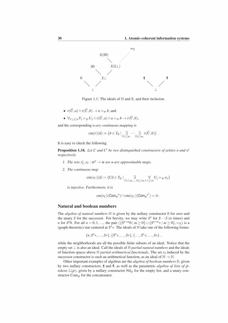
30 1. Atomic-coherent information systems
⊥
0 S⊥
S0 S(S⊥)
S(S0)
∞S
...................................................
...................................................
...................................................
.............................................
.......................................
.
.
.
.
.
.
.
.
.
.
.
.
.
.
.
.
.
.
.
⊥
tt ff....................................................
....................................................
Figure 1.1: The ideals of N and B, and their inclusion.
• r(~U ,a)∧ r(~U ,b)→ a≍σ b, and
• ∀1≤ j≤n Vj ≻ρ U j ∧ r(~U ,a)∧a≻σ b→ r(~V ,b),
and the corresponding n-ary continuous mapping is
cm(r)(~u)≔ b ∈ Tσ | ∃U1⊆u1
· · · ∃Un⊆un
r(~U ,b) .
It is easy to check the following.
Proposition 1.34. Let C and C′ be two distinguished constructors of arities n and n′
respectively.
1. The sets r∗C,rC : αn → α are n-ary approximable maps.
2. The continuous map
cm(rC)(~u) = C~a ∈ Tα | ∃U1⊆u1,...,Un⊆un
∀1≤ j≤n
U j ≻α a j
is injective. Furthermore, it is
cm(rC)(Conαn)∩ cm(rC′)(Conα
n′) = ∅ .
Natural and boolean numbers
The algebra of natural numbers N is given by the nullary constructor 0 for zero and
the unary S for the successor. For brevity, we may write Sn for S · · ·S (n times) and
n for Sn0. For all n = 0,1, . . ., the pair (Sn+m0 | m≥ 0∪Sn+m∗ | m≥ 0,≍N) is a
(graph-theoretic) star centered at Sn∗. The ideals of N take one of the following forms:
n,Sn∗, . . . ,S∗,Sn∗, . . . ,S∗,. . . ,Sn∗, . . . ,S∗ ,
while the neighborhoods are all the possible finite subsets of an ideal. Notice that the
empty set⊥ is also an ideal. Call the ideals of N partial natural numbers and the ideals
of function spaces above N partial arithmetical functionals. The set rS induced by the
successor constructor is such an arithmetical function, as an ideal of N→ N.
Other important examples of algebras are the algebra of boolean numbers B, given
by two nullary constructors, tt and ff, as well as the parametric algebra of lists of ρ-
tokens L(ρ), given by a nullary constructor Nilρ for the empty list, and a unary con-
structor Consρ for the concatenator.
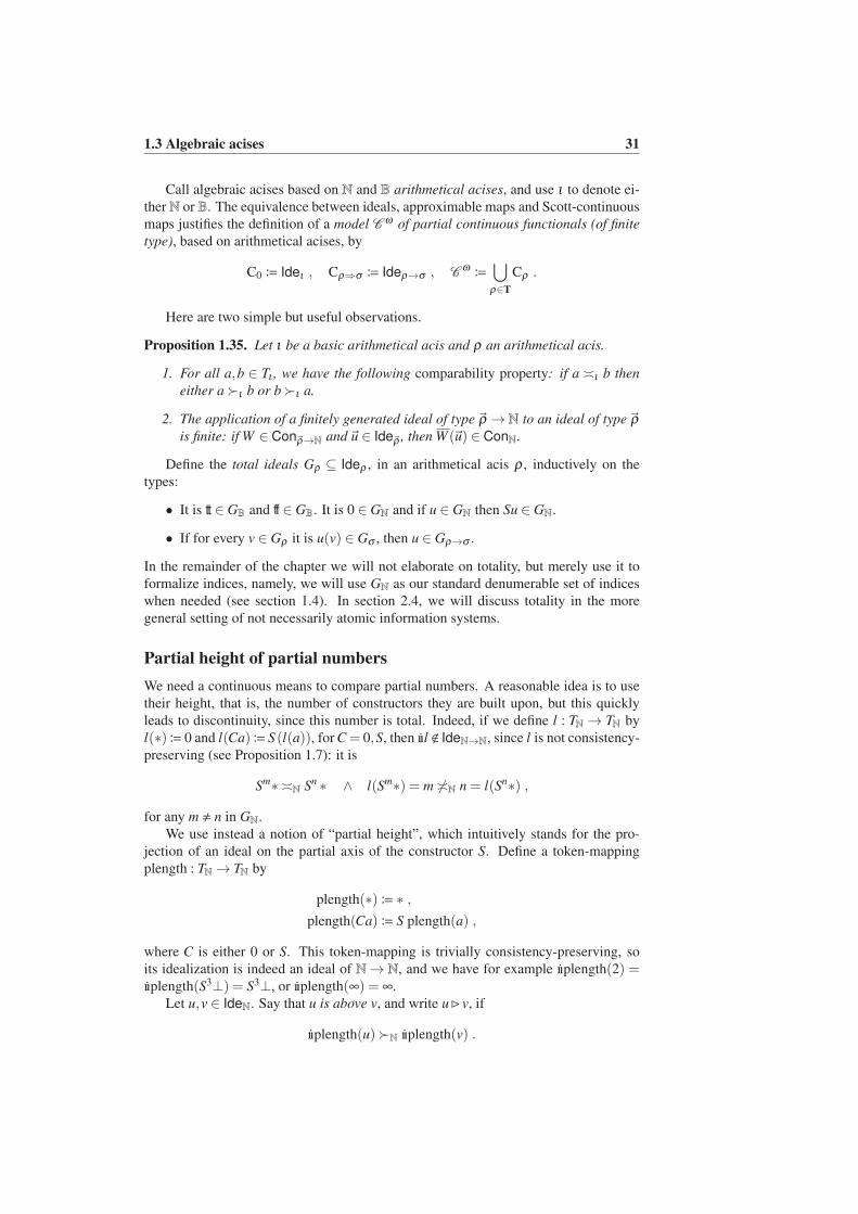
1.3 Algebraic acises 31
Call algebraic acises based on N and B arithmetical acises, and use ι to denote ei-
therN or B. The equivalence between ideals, approximable maps and Scott-continuous
maps justifies the definition of a model C ω of partial continuous functionals (of finite
type), based on arithmetical acises, by
C0 ≔ Ideι , Cρ⇒σ ≔ Ideρ→σ , Cω≔⋃
ρ∈T
Cρ .
Here are two simple but useful observations.
Proposition 1.35. Let ι be a basic arithmetical acis and ρ an arithmetical acis.
1. For all a,b ∈ Tι , we have the following comparability property: if a ≍ι b then
either a≻ι b or b≻ι a.
2. The application of a finitely generated ideal of type ~ρ → N to an ideal of type ~ρis finite: if W ∈ Con~ρ→N and~u ∈ Ide~ρ , then W (~u) ∈ ConN.
Define the total ideals Gρ ⊆ Ideρ , in an arithmetical acis ρ , inductively on the
types:
• It is tt ∈ GB and ff ∈ GB. It is 0 ∈ GN and if u ∈ GN then Su ∈ GN.
• If for every v ∈ Gρ it is u(v) ∈ Gσ , then u ∈ Gρ→σ .
In the remainder of the chapter we will not elaborate on totality, but merely use it to
formalize indices, namely, we will use GN as our standard denumerable set of indices
when needed (see section 1.4). In section 2.4, we will discuss totality in the more
general setting of not necessarily atomic information systems.
Partial height of partial numbers
We need a continuous means to compare partial numbers. A reasonable idea is to use
their height, that is, the number of constructors they are built upon, but this quickly
leads to discontinuity, since this number is total. Indeed, if we define l : TN→ TN by
l(∗)≔ 0 and l(Ca)≔ S (l(a)), for C = 0,S, then ııl < IdeN→N, since l is not consistency-
preserving (see Proposition 1.7): it is
Sm∗ ≍N Sn ∗ ∧ l(Sm∗) = m 6≍N n = l(Sn∗) ,
for any m , n in GN.
We use instead a notion of “partial height”, which intuitively stands for the pro-
jection of an ideal on the partial axis of the constructor S. Define a token-mapping
plength : TN→ TN by
plength(∗)≔ ∗ ,
plength(Ca)≔ S plength(a) ,
where C is either 0 or S. This token-mapping is trivially consistency-preserving, so
its idealization is indeed an ideal of N→ N, and we have for example ııplength(2) =ııplength(S3⊥) = S3⊥, or ııplength(∞) = ∞.
Let u,v ∈ IdeN. Say that u is above v, and write u⊲ v, if
ııplength(u)≻N ııplength(v) .
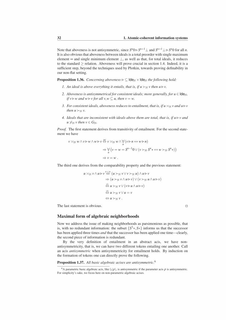
32 1. Atomic-coherent information systems
Note that aboveness is not antisymmetric, since Sn0⊲Sn+1⊥ and Sn+1⊥⊲Sn0 for all n.
It is also obvious that aboveness between ideals is a total preorder with single maximum
element ∞ and single minimum element ⊥, as well as that, for total ideals, it reduces
to the standard ≥ relation. Aboveness will prove crucial in section 1.4. Indeed, it is a
sufficient step, beyond the techniques used by Plotkin, towards proving definability in
our non-flat setting.
Proposition 1.36. Concerning aboveness ⊲⊆ IdeN× IdeN the following hold:
1. An ideal is above everything it entails, that is, if u≻N v then u⊲ v.
2. Aboveness is antisymmetrical for consistent ideals; more generally, for u∈ IdeN,
if v⊲w and w⊲ v for all v,w⊆ u, then v = w.
3. For consistent ideals, aboveness reduces to entailment, that is, if u≍N v and u⊲v
then u≻N v.
4. Ideals that are inconsistent with ideals above them are total, that is, if u⊲ v and
u 6≍N v then v ∈ GN.
Proof. The first statement derives from transitivity of entailment. For the second state-
ment we have
v≍N w∧ v⊲w∧w⊲ vdef⇔ v≍N w∧∀
n(v⊲n↔ w⊲n)
⇒ ∀n
(
v = w = Sn−10∨ (v≻N Sn∗↔ w≻N Sn∗))
⇒ v = w .
The third one derives from the comparability property and the previous statement:
u≍N v∧u⊲ vP. 1.35⇔ (u≻N v∨ v≻N u)∧u⊲ v
⇒ (u≻N v∧u⊲ v)∨ (v≻N u∧u⊲ v)(2)⇔ u≻N v∨ (v⊲u∧u⊲ v)(3)⇔ u≻N v∨u = v
⇔ u≻N v .
The last statement is obvious.
Maximal form of algebraic neighborhoods
Now we address the issue of making neighborhoods as parsimonious as possible, that
is, with no redundant information: the subset S3∗,S∗ informs us that the successor
has been applied three times and that the successor has been applied one time—clearly,
the second piece of information is redundant.
By the very definition of entailment in an abstract acis, we have non-
antisymmetricity, that is, we can have two different tokens entailing one another. Call
an acis antisymmetric when antisymmetricity for entailment holds. By induction on
the formation of tokens one can directly prove the following.
Proposition 1.37. All basic algebraic acises are antisymmetric.6
6A parametric basic algebraic acis, like L(ρ), is antisymmetric if the parameter acis ρ is antisymmetric.
For simplicity’s sake, we focus here on non-parametric algebraic acises.
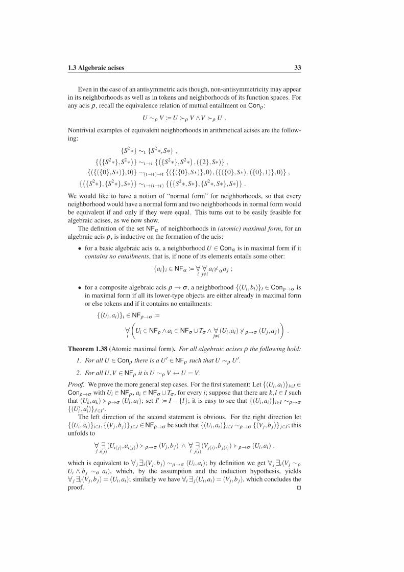
1.3 Algebraic acises 33
Even in the case of an antisymmetric acis though, non-antisymmetricity may appear
in its neighborhoods as well as in tokens and neighborhoods of its function spaces. For
any acis ρ , recall the equivalence relation of mutual entailment on Conρ :
U ∼ρ V ≔U ≻ρ V ∧V ≻ρ U .
Nontrivial examples of equivalent neighborhoods in arithmetical acises are the follow-
ing:
S2∗ ∼ι S2∗,S∗ ,
(
S2∗,S2∗)
∼ι→ι (
S2∗,S2∗)
,(2,S∗) ,
((0,S∗),0) ∼(ι→ι)→ι ((0,S∗),0) ,((0,S∗) ,(0,1),0) ,
(
S2∗,S2∗,S∗)
∼ι→(ι→ι) (
S2∗,S∗,S2∗,S∗,S∗)
.
We would like to have a notion of “normal form” for neighborhoods, so that every
neighborhood would have a normal form and two neighborhoods in normal form would
be equivalent if and only if they were equal. This turns out to be easily feasible for
algebraic acises, as we now show.
The definition of the set NFα of neighborhoods in (atomic) maximal form, for an
algebraic acis ρ , is inductive on the formation of the acis:
• for a basic algebraic acis α , a neighborhood U ∈ Conα is in maximal form if it
contains no entailments, that is, if none of its elements entails some other:
aii ∈ NFα ≔ ∀i∀j,i
ai 6≻α a j ;
• for a composite algebraic acis ρ → σ , a neighborhood (Ui,bi)i ∈ Conρ→σ is
in maximal form if all its lower-type objects are either already in maximal form
or else tokens and if it contains no entailments:
(Ui,ai)i ∈ NFρ→σ ≔
∀i
(
Ui ∈ NFρ ∧ai ∈ NFσ ∪Tσ ∧ ∀j,i(Ui,ai) 6≻ρ→σ (U j,a j)
)
.
Theorem 1.38 (Atomic maximal form). For all algebraic acises ρ the following hold:
1. For all U ∈ Conρ there is a U ′ ∈ NFρ such that U ∼ρ U ′.
2. For all U,V ∈ NFρ it is U ∼ρ V ↔U =V .
Proof. We prove the more general step cases. For the first statement: Let (Ui,ai)i∈I ∈Conρ→σ with Ui ∈ NFρ , ai ∈ NFσ ∪Tσ , for every i; suppose that there are k, l ∈ I such
that (Uk,ak) ≻ρ→σ (Ul ,al); set I′ ≔ I−l; it is easy to see that (Ui,ai)i∈I ∼ρ→σ
(U ′i ,a
′i)i′∈I′ .
The left direction of the second statement is obvious. For the right direction let
(Ui,ai)i∈I ,(Vj,b j) j∈J ∈NFρ→σ be such that (Ui,ai)i∈I ∼ρ→σ (Vj,b j) j∈J ; this
unfolds to
∀j∃
i( j)(Ui( j),ai( j))≻ρ→σ (Vj,b j) ∧ ∀
i∃j(i)
(Vj(i),b j(i))≻ρ→σ (Ui,ai) ,
which is equivalent to ∀ j∃i(Vj,b j) ∼ρ→σ (Ui,ai); by definition we get ∀ j∃i(Vj ∼ρ
Ui ∧ b j ∼σ ai), which, by the assumption and the induction hypothesis, yields
∀ j∃i(Vj,b j) = (Ui,ai); similarly we have ∀i∃ j(Ui,ai) = (Vj,b j), which concludes the
proof.
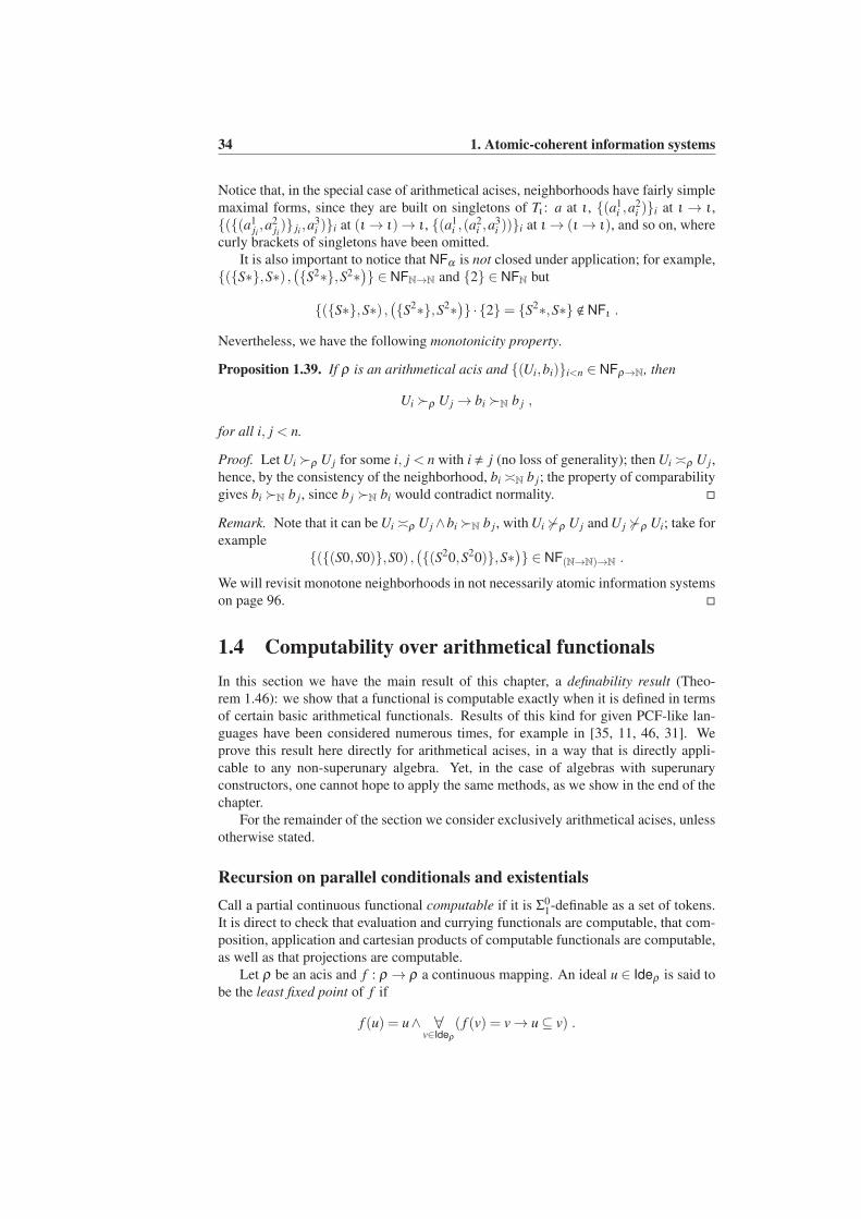
34 1. Atomic-coherent information systems
Notice that, in the special case of arithmetical acises, neighborhoods have fairly simple
maximal forms, since they are built on singletons of Tι : a at ι , (a1i ,a
2i )i at ι → ι ,
((a1ji,a2
ji) ji ,a
3i )i at (ι → ι)→ ι , (a1
i ,(a2i ,a
3i ))i at ι → (ι → ι), and so on, where
curly brackets of singletons have been omitted.
It is also important to notice that NFα is not closed under application; for example,
(S∗,S∗) ,(
S2∗,S2∗)
∈ NFN→N and 2 ∈ NFN but
(S∗,S∗) ,(
S2∗,S2∗)
· 2= S2∗,S∗ < NFι .
Nevertheless, we have the following monotonicity property.
Proposition 1.39. If ρ is an arithmetical acis and (Ui,bi)i<n ∈ NFρ→N, then
Ui ≻ρ U j → bi ≻N b j ,
for all i, j < n.
Proof. Let Ui ≻ρ U j for some i, j < n with i , j (no loss of generality); then Ui ≍ρ U j,
hence, by the consistency of the neighborhood, bi ≍N b j; the property of comparability
gives bi ≻N b j, since b j ≻N bi would contradict normality.
Remark. Note that it can be Ui ≍ρ U j∧bi ≻N b j, with Ui 6≻ρ U j and U j 6≻ρ Ui; take for
example
((S0,S0),S0) ,(
(S20,S20),S∗)
∈ NF(N→N)→N .
We will revisit monotone neighborhoods in not necessarily atomic information systems
on page 96.
1.4 Computability over arithmetical functionals
In this section we have the main result of this chapter, a definability result (Theo-
rem 1.46): we show that a functional is computable exactly when it is defined in terms
of certain basic arithmetical functionals. Results of this kind for given PCF-like lan-
guages have been considered numerous times, for example in [35, 11, 46, 31]. We
prove this result here directly for arithmetical acises, in a way that is directly appli-
cable to any non-superunary algebra. Yet, in the case of algebras with superunary
constructors, one cannot hope to apply the same methods, as we show in the end of the
chapter.
For the remainder of the section we consider exclusively arithmetical acises, unless
otherwise stated.
Recursion on parallel conditionals and existentials
Call a partial continuous functional computable if it is Σ01-definable as a set of tokens.
It is direct to check that evaluation and currying functionals are computable, that com-
position, application and cartesian products of computable functionals are computable,
as well as that projections are computable.
Let ρ be an acis and f : ρ → ρ a continuous mapping. An ideal u ∈ Ideρ is said to
be the least fixed point of f if
f (u) = u∧ ∀v∈Ideρ
( f (v) = v→ u⊆ v) .
1.4 Computability over arithmetical functionals 35
Proposition 1.40. Let ρ be an acis and f : ρ → ρ a continuous mapping. The mapping
f has a least fixed point given by the equation
Y( f ) =⋃
n∈GN
f n(⊥) .
Proof. Since f is continuous, it is monotone and commutes with directed unions. By
monotonicity,
⊥⊆ f (⊥)⊆ ·· · ⊆ f n(⊥)⊆ ·· · ,
which yields u≔⋃
n∈GNf n(⊥) ∈ Ideρ ; by commutativity with directed unions,
f (u) = f (⋃
n∈GN
f n(⊥)) =⋃
n∈GN
f ( f n(⊥)) =⋃
n∈GN
f n+1(⊥) = u .
So u is a fixed point. Let v be another fixed point of f ; we have
⊥⊆ v⇒ f (⊥)⊆ f (v) = v⇒ ·· · ⇒ f n(⊥)⊆ v⇒ ·· · ,
which yields u =⋃
n∈GNf n(⊥)⊆ v, so u is the least fixed point.
Proposition 1.41. The least fixed point functional Y : (ρ → ρ)→ ρ is continuous and
computable for any ρ .
Proof. For monotonicity, if f ⊆ g, then trivially⋃
n∈GNf n(⊥)⊆
⋃
n∈GNgn(⊥). For the
principle of finite support, let b ∈ Y( f ), that is, b ∈⋃
n∈GNf n(⊥); equivalently,
∃n∈GN
b ∈ f n(⊥)PFS⇒ ∃
n∈GN∃
W⊆ f f
b ∈Wn(⊥)
def⇔ ∃
W⊆ f f
b ∈⋃
n∈GN
Wn(⊥) ,
so ∃W⊆ f f b ∈ Y(W ). For Σ01-definability, let (U,a) ∈ Yρ , that is, a ∈ Yρ(U); then
equivalently
a ∈⋃
n∈GN
Un(⊥)
def⇔ ∃
n∈GN
a ∈Un(⊥)
P. 1.17(4)⇔ ∃
n∈GN
a ∈Un∅def⇔ ∃
n∈GN
Un∅≻ρ a ;
but this is equivalent to the formula
∃n∈GN
∃V0
· · ·∃Vn
(
V0 = ∅∧ ∀i<n
(Vi+1 =UVi)∧Vn ≻ρ a
)
,
which is a Σ01-expression by Proposition 1.17(5).
Define the parallel conditional functional pcond : B→ N→ N→ N by
pcond(p,u,v)≔
u , p = tt ,
v , p = ff ,
u∩ v , p =⊥ .
Proposition 1.42. The parallel conditional functional is continuous and computable.
36 1. Atomic-coherent information systems
Proof. For monotonicity: Let u⊆ u′ and v⊆ v′; we distinguish cases according to the
boolean values:
pcond(tt,u,v) = u⊆ u′ = pcond(tt,u′,v′) ,
pcond(ff,u,v) = v⊆ v′ = pcond(ff,u′,v′) ,
pcond(⊥,u,v) = u∩ v⊆ u′∩ v′ = pcond(⊥,u′,v′) ,
pcond(⊥,u,v) = u∩ v⊆ u⊆ u′ = pcond(tt,u′,v′) ,
pcond(⊥,u,v) = u∩ v⊆ v⊆ v′ = pcond(ff,u′,v′) .
For the principle of finite support: if a ∈ pcond(tt,u,v) then a ∈ pcond(tt,a,∅); if
a ∈ pcond(ff,u,v) then a ∈ pcond(ff,∅,a); finally, if a ∈ pcond(⊥,u,v) then a ∈pcond(∅,a,a). For Σ0
1-definability, let (P,U,V,a)∈ pcond, that is, a∈ pcond(P,U ,V );this is equivalent to the formula
(P≻B tt∧U ≻N a)∨ (P≻B ff∧V ≻N a)∨ (P = ∅∧U ≻N a∧V ≻N a) ,
which is a Σ01-expression.
Define the (parallel) existential functional exist : (N→ B)→ B by
exist( f ) =
ff , ∃n∈GN ( f (Sn⊥) = ff∧∀k≤n f (k) = ff) ,
tt , ∃n∈GN f (n) = tt ,
⊥ , otherwise .
Proposition 1.43. The existential functional is continuous and computable.
Proof. For monotonicity: Let f , f ′ ∈ IdeN→B be such that f ⊆ f ′. We distinguish three
cases: In case ∃n∈GN ( f (Sn⊥) = ff∧∀k≤n f (k) = ff), then, by definition,
∃n∈GN
(
∃U∈ConN
(Sn⊥≻N U ∧ (U, ff) ∈ f )∧ ∀k≤n
∃Vk∈ConN
(k ≻N Vk ∧ (Vk, ff) ∈ f )
)
;
since f ⊆ f ′, we trivially get
∃n∈GN
(
∃U∈ConN
(
Sn⊥≻N U ∧ (U, ff) ∈ f ′)
∧ ∀k≤n
∃Vk∈ConN
(
k ≻N Vk ∧ (Vk, ff) ∈ f ′)
)
,
which in turn means that ∃n∈GN ( f ′(Sn⊥) = ff∧∀k≤n f ′(k) = ff), so exist( f ) =exist( f ′) = ff. In case ∃n∈GN f (n) = tt, we have
∃n∈GN
∃U∈ConN
(
n≻N U ∧ (U, tt) ∈ f ⊆ f ′)
,
which gives ∃n∈GN f ′(n) = tt, so exist( f ) = exist( f ′) = tt. Finally, in case exist( f ) =⊥,
it is obviously exist( f )⊆ exist( f ′) for any possible value of the latter.
For the principle of finite support: Let b ∈ exist( f ); if there exists an n ∈ GN such
that f (Sn⊥) = ff∧∀k≤n f (k) = ff then b∈ exist((Sn∅, ff)); if there exists an n∈GN such
that f (n) = tt then b ∈ exist((n, tt)) (the case b ∈ ⊥ is absurd).
For Σ01-definability: Let ((Ui,bi)i≤m,b) ∈ exist, that is, b ∈ exist((Ui,bi)i≤m);
this is equivalent to the formula(
tt≻B b∧ ∃n∈GN
(Ui,bi)i≤m ≻N→B (Sn0, tt)
)
∨
(
ff≻B b∧ ∃n∈GN
(
(Ui,bi)i≤m ≻N→B (Sn∅, ff)∧ ∀
k≤n(Ui,bi)i≤m ≻N→B (S
k0, ff)
))
,
1.4 Computability over arithmetical functionals 37
which is a Σ01-expression.
In terms of pcond and exist we can easily define the following:
1. The conditional functional cond : B→ N→ N→ N defined by
cond(p,u,v)≔ pcond(p,pcond(p,u,⊥),pcond(p,⊥,v)) ,
which can be unfolded to
cond(p,u,v) =
u , p = tt ,
v , p = ff ,
⊥ , p =⊥ .
Note that pcond(p,u,v) = cond(p,u,v) if and only if u∩ v =⊥.
2. The disjunction functional or : B→ B→ B defined by
or(p,q)≔ pcond(p, tt,q) ,
which unfolds to
or(p,q)≔
tt , p = tt∨q = tt ,
ff , p = q = ff ,
⊥ , otherwise .
3. The conjunction functional and : B→ B→ B defined by
and(p,q)≔ pcond(p,q, ff) ,
which unfolds to
and(p,q)≔
tt , p = q = tt ,
ff , p = ff∨q = ff ,
⊥ , otherwise .
4. The negation functional not : B→ B defined by
not(p)≔ pcond(p, ff, tt) ,
which unfolds to
not(p)≔
tt , p = ff ,
ff , p = tt ,
⊥ , otherwise .
5. The implication functional implies : B→ B→ B defined by
implies(p,q)≔ or(not(p),q) ,
which unfolds to
implies(p,q)≔
tt , p = ff∨q = tt ,
ff , p = tt∧q = ff ,
⊥ , otherwise .
All of these are continuous and computable functionals since they are defined by
pcond. The p-ary generalization of or we will denote by ORpi=1.
38 1. Atomic-coherent information systems
Enumeration and inconsistency functionals
To make case distinctions in subsequent proofs less branching, we hereafter adopt the
following convention: let ρ , σ and τ be arithmetical acises; a functional f : ρ → N→σ → τ that satisfies f (u,x,v) =⊥ for x < GN, will be informally typed by ρ → GN→σ → τ , and will be treated only on its arguments where x is total.
For every arithmetical acis we fix an enumeration of neighborhoods Unn∈GN ,
such that (i) U0 = ∅ holds, and (ii) the following are primitive recursive relations:
Un ≍ρ Um, Un ≻ρ Um, Un ·Um = Uk (for appropriate types), and Un ∪Um = Uk, with
k = 0 if Un 6≍ρ Um. In the following we may write b for singleton neighborhoods b,whenever we want to stress that they behave as tokens.
Define the conditional extension functional (also continuous union, see note on
page 47) condext : N→ GN→ N by
condext(v,n)≔
v , bn ∈ v ,
bn , otherwise .
The condext operator extends bn to v whenever this is allowed.
Proposition 1.44. The conditional extension functional is continuous and computable.
Proof. For monotonicity: Let v,v′ ∈ IdeN, with v ⊆ v′. In case bn ∈ v, then bn ∈ v′
as well, so condext(v,n) = v ⊆ v′ = condext(v′,n). In case bn < v, then either bn ∈ v′
and so condext(v,n) = bn ⊆ v′ = condext(v′,n), or bn < v′ and so condext(v,n) = bn =condext(v′,n).
For the principle of finite support, let b∈ condext(v,n). If bn ∈ v then b∈ v as well,
and b ∈ condext(b∪bn,n). If bn < v then b ∈ bn, and b ∈ condext(bn,n).For Σ0
1-definability, consider a token (V,N,b) ∈ condext. This means that b ∈condext(V ,N), which is equivalent to the formula
∃n∈GN
(N ≻N n∧ (V 6≻N bn∨V ≻N b∨bn ≻N b)) ;
this is a Σ01-expression.
Proposition 1.45. Let ρ be an arithmetical acis.
1. There exists an enumeration functional enρ : GN→ N→ ρ , with the properties
enρ(m,x) =Um, when x < GN ,
enρ(m,n) =Un, when Un ≻ρ Um .
2. There exists an inconsistency functional incnsρ : ρ →GN→B, with the property
incnsρ(u,n) =
tt , u 6≍ρ Un ,
ff , u≻ρ Un .
The inconsistency functionals concern application: let σ be an arithmetical acis and
(Un,bn) a token of a partial continuous functional v of type ρ → σ ; the only case where
the token may contribute the information bn to the value v(u) is when incnsρ(u,n) is
ff. In order to define the functionals incnsρ , we will need the enumeration functionals,
that enumerate all finitely generated extensions of Um, for Um ∈ Conρ .
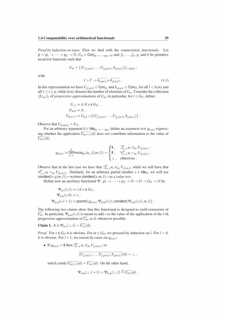
1.4 Computability over arithmetical functionals 39
Proof by induction on types. First we deal with the enumeration functionals. Let
ρ = ρ1 → ·· · → ρp → N, Um ∈ Conρ1→···→ρp→N and f1, . . . , fp, g, and h be primitive
recursive functions such that
Um = (U f1(m,l), . . . ,U fp(m,l),bg(m,l))l<h(m) ,
with
l > l′→ bg(m,l)⊲bg(m,l′) . (1.1)
In this representation we have U fi(m,l) ∈Conρiand bg(m,l) ∈ConN, for all l < h(m) and
all 1≤ i≤ p, while h(m) denotes the number of elements of Um. Consider the collection
Um,ll of progressive approximations of Um; in particular, for l ∈ GN, define:
Ux,l ≔ ∅ if x < GN ,
Um,0 ≔ ∅ ,
Um,l+1 ≔Um,l ∪(U f1(m,l), . . . ,U fp(m,l),bg(m,l)) .
Observe that Um,h(m) =Um.
For an arbitrary argument ~u ∈ Ideρ1→···→ρp , define an argument test q~u,m,l express-
ing whether the application Um,l+1(~u) does not contribute information to the value of
Um,l(~u):
q~u,m,l ≔
p
ORi=1
incnsρi(ui, fi(m, l)) =
tt , ∃pi=1 ui 6≍ρi
U fi(m,l) ,
ff , ∀pi=1 ui ≻ρi
U fi(m,l) ,
⊥ , otherwise .
Observe that in the last case we have that ∃pi=1 ui 6≻ρi
U fi(m,l) while we still have that
∀pi=1 ui ≍ρi
U fi(m,l). Similarly, for an arbitrary partial number v ∈ IdeN, we will use
condext(v,g(m, l))—written condext(v,m, l)—as a value test.
Define now an auxiliary functional Ψ : ρ1 → ·· · → ρp → N→ N→ GN→ N by
Ψ~u,x(v, l)≔ v if x < GN ,
Ψ~u,m(v,0)≔ v ,
Ψ~u,m(v, l +1)≔ pcond(
q~u,m,l ,Ψ~u,m(v, l),condext(Ψ~u,m(v, l),m, l))
.
The following two claims show that this functional is designed to yield extensions of
Um. In particular, Ψ~u,m(v, l) is meant to add v to the value of the application of the l-th
progressive approximation of Um, to~u, whenever possible.
Claim 1. It is Ψ~u,x(⊥, l) =Ux,l(~u).
Proof. For x < GN it is obvious. For m ∈ GN, we proceed by induction on l. For l = 0,
it is obvious. For l +1, we reason by cases on q~u,m,l :
• If q~u,m,l = tt then ∃pi=1 ui 6≍ρi
U fi(m,l), so
(U f1(m,l), . . . ,U fp(m,l),bg(m,l))(~u) =⊥ ,
which yields Um,l+1(~u) =Um,l(~u). On the other hand,
Ψ~u,m(⊥, l +1) = Ψ~u,m(⊥, l)IH=Um,l(~u) .
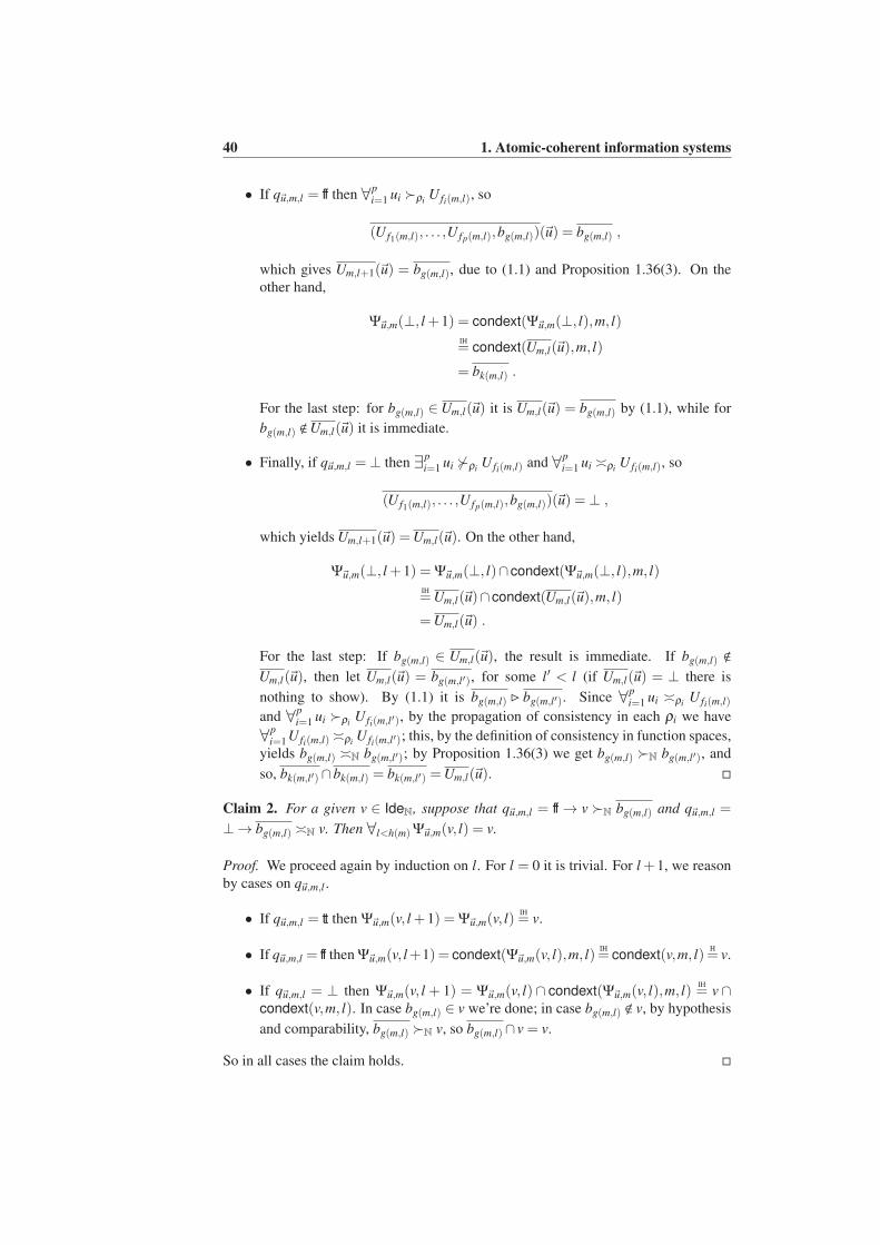
40 1. Atomic-coherent information systems
• If q~u,m,l = ff then ∀pi=1 ui ≻ρi
U fi(m,l), so
(U f1(m,l), . . . ,U fp(m,l),bg(m,l))(~u) = bg(m,l) ,
which gives Um,l+1(~u) = bg(m,l), due to (1.1) and Proposition 1.36(3). On the
other hand,
Ψ~u,m(⊥, l +1) = condext(Ψ~u,m(⊥, l),m, l)IH= condext(Um,l(~u),m, l)
= bk(m,l) .
For the last step: for bg(m,l) ∈Um,l(~u) it is Um,l(~u) = bg(m,l) by (1.1), while for
bg(m,l) <Um,l(~u) it is immediate.
• Finally, if q~u,m,l =⊥ then ∃pi=1 ui 6≻ρi
U fi(m,l) and ∀pi=1 ui ≍ρi
U fi(m,l), so
(U f1(m,l), . . . ,U fp(m,l),bg(m,l))(~u) =⊥ ,
which yields Um,l+1(~u) =Um,l(~u). On the other hand,
Ψ~u,m(⊥, l +1) = Ψ~u,m(⊥, l)∩condext(Ψ~u,m(⊥, l),m, l)IH=Um,l(~u)∩condext(Um,l(~u),m, l)
=Um,l(~u) .
For the last step: If bg(m,l) ∈ Um,l(~u), the result is immediate. If bg(m,l) <
Um,l(~u), then let Um,l(~u) = bg(m,l′), for some l′ < l (if Um,l(~u) = ⊥ there is
nothing to show). By (1.1) it is bg(m,l) ⊲ bg(m,l′). Since ∀pi=1 ui ≍ρi
U fi(m,l)
and ∀pi=1 ui ≻ρi
U fi(m,l′), by the propagation of consistency in each ρi we have
∀pi=1 U fi(m,l) ≍ρi
U fi(m,l′); this, by the definition of consistency in function spaces,
yields bg(m,l) ≍N bg(m,l′); by Proposition 1.36(3) we get bg(m,l) ≻N bg(m,l′), and
so, bk(m,l′)∩bk(m,l) = bk(m,l′) =Um,l(~u).
Claim 2. For a given v ∈ IdeN, suppose that q~u,m,l = ff → v ≻N bg(m,l) and q~u,m,l =
⊥→ bg(m,l) ≍N v. Then ∀l<h(m) Ψ~u,m(v, l) = v.
Proof. We proceed again by induction on l. For l = 0 it is trivial. For l +1, we reason
by cases on q~u,m,l .
• If q~u,m,l = tt then Ψ~u,m(v, l +1) = Ψ~u,m(v, l)IH= v.
• If q~u,m,l = ff then Ψ~u,m(v, l+1) = condext(Ψ~u,m(v, l),m, l)IH= condext(v,m, l)
H= v.
• If q~u,m,l = ⊥ then Ψ~u,m(v, l + 1) = Ψ~u,m(v, l)∩ condext(Ψ~u,m(v, l),m, l)IH= v∩
condext(v,m, l). In case bg(m,l) ∈ v we’re done; in case bg(m,l) < v, by hypothesis
and comparability, bg(m,l) ≻N v, so bg(m,l)∩ v = v.
So in all cases the claim holds.
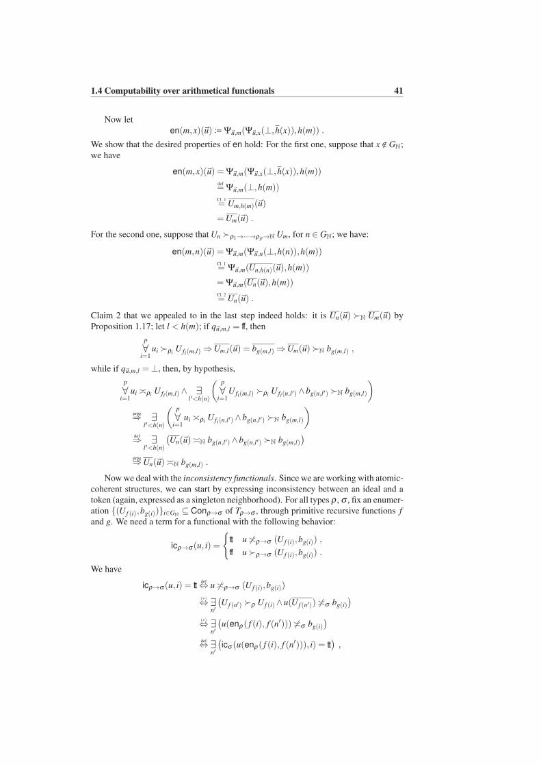
1.4 Computability over arithmetical functionals 41
Now let
en(m,x)(~u)≔Ψ~u,m(Ψ~u,x(⊥,h(x)),h(m)) .
We show that the desired properties of en hold: For the first one, suppose that x < GN;
we have
en(m,x)(~u) = Ψ~u,m(Ψ~u,x(⊥,h(x)),h(m))def= Ψ~u,m(⊥,h(m))Cl. 1= Um,h(m)(~u)
=Um(~u) .
For the second one, suppose that Un ≻ρ1→···→ρp→N Um, for n ∈ GN; we have:
en(m,n)(~u) = Ψ~u,m(Ψ~u,n(⊥,h(n)),h(m))Cl. 1= Ψ~u,m(Un,h(n)(~u),h(m))
= Ψ~u,m(Un(~u),h(m))Cl. 2= Un(~u) .
Claim 2 that we appealed to in the last step indeed holds: it is Un(~u) ≻N Um(~u) by
Proposition 1.17; let l < h(m); if q~u,m,l = ff, then
p
∀i=1
ui ≻ρiU fi(m,l)⇒Um,l(~u) = bg(m,l)⇒Um(~u)≻N bg(m,l) ,
while if q~u,m,l =⊥, then, by hypothesis,
p
∀i=1
ui ≍ρiU fi(m,l)∧ ∃
l′<h(n)
(p
∀i=1
U fi(m,l) ≻ρiU fi(n,l′)∧bg(n,l′) ≻N bg(m,l)
)
prpg
⇒ ∃l′<h(n)
(p
∀i=1
ui ≍ρiU fi(n,l′)∧bg(n,l′) ≻N bg(m,l)
)
def⇒ ∃
l′<h(n)
(
Un(~u)≍N bg(n,l′)∧bg(n,l′) ≻N bg(m,l)
)
prpg
⇒Un(~u)≍N bg(m,l) .
Now we deal with the inconsistency functionals. Since we are working with atomic-
coherent structures, we can start by expressing inconsistency between an ideal and a
token (again, expressed as a singleton neighborhood). For all types ρ , σ , fix an enumer-
ation (U f (i),bg(i))i∈GN ⊆ Conρ→σ of Tρ→σ , through primitive recursive functions f
and g. We need a term for a functional with the following behavior:
icρ→σ (u, i) =
tt u 6≍ρ→σ (U f (i),bg(i)) ,
ff u≻ρ→σ (U f (i),bg(i)) .
We have
icρ→σ (u, i) = ttdef⇔ u 6≍ρ→σ (U f (i),bg(i))
(∗)⇔ ∃
n′
(
U f (n′) ≻ρ U f (i)∧u(U f (n′)) 6≍σ bg(i)
)
(∗)⇔ ∃
n′
(
u(enρ( f (i), f (n′))) 6≍σ bg(i)
)
def⇔ ∃
n′
(
icσ (u(enρ( f (i), f (n′))), i) = tt)
,
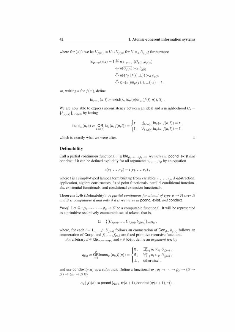
42 1. Atomic-coherent information systems
where for (∗)’s we let U f (n′) ≔U ∪U f (i), for U ≍ρ U f (i); furthermore
icρ→σ (u, i) = ffdef⇔ u≻ρ→σ (U f (i),bg(i))
⇔ u(U f (i))≻σ bg(i)
def⇔ u(enρ( f (i),⊥))≻σ bg(i)
def⇔ icσ (u(enρ( f (i),⊥)), i) = ff ,
so, writing n for f (n′), define
icρ→σ (u, i)≔ exist(λn icσ (u(enρ( f (i),n)), i)) .
We are now able to express inconsistency between an ideal and a neighborhood Un =b j(n,l)l<h(n), by letting
incnsρ(u,n)≔ ORl<h(n)
icρ(u, j(n, l)) =
tt , ∃l<h(n) icρ(u, j(n, l)) = tt ,
ff , ∀l<h(n) icρ(u, j(n, l)) = ff ,
which is exactly what we were after.
Definability
Call a partial continuous functional u ∈ Ideρ1→···→ρp→N recursive in pcond, exist and
condext if it can be defined explicitly for all arguments v1, . . . ,vp by an equation
u(v1, . . . ,vp) = t(v1, . . . ,vp) ,
where t is a simply-typed lambda term built up from variables v1, . . . ,vp, λ -abstraction,
application, algebra constructors, fixed point functionals, parallel conditional function-
als, existential functionals, and conditional extension functionals.
Theorem 1.46 (Definability). A partial continuous functional of type ρ → N over N
and B is computable if and only if it is recursive in pcond, exist, and condext.
Proof. Let Ω : ρ1 → ·· · → ρp → N be a computable functional. It will be represented
as a primitive recursively enumerable set of tokens, that is,
Ω = (U f1(n), . . . ,U fp(n),bg(n))n∈GN ,
where, for each i = 1, . . . , p, U fi(n) follows an enumeration of Conρi, bg(n) follows an
enumeration of ConN, and f1, . . . , fp,g are fixed primitive recursive functions.
For arbitrary~u ∈ Ideρ1→···→ρp and v ∈ IdeN, define an argument test by
q~u,n ≔p
ORi=1
incnsρi(ui, fi(n)) =
tt , ∃pi=1 ui 6≍ρi
U fi(n) ,
ff , ∀pi=1 ui ≻ρi
U fi(n) ,
⊥ , otherwise ,
and use condext(v,n) as a value test. Define a functional ω : ρ1 → ·· · → ρp → (N→N)→ GN→ N by
ω~u(ψ)(n)≔ pcond(
q~u,n,ψ(n+1),condext(ψ(n+1),n))
.
1.4 Computability over arithmetical functionals 43
We show that Ω(~u) = Y(ω~u)(0). In particular, we show that both recursion on ω~u at 0
and Ω(~u) entail the very same information, that is,
∀b∈TN
(Ω(~u)≻N b↔ Y(ω~u)(0)≻N b) .
For the right direction, suppose that there exists a token b∈ TN such that Ω(~u)≻N b.
This means that
∃n∈GN
(p
∀i=1
ui ≻ρiU fi(n)∧bg(n) ≻N b
)
. (1.2)
We claim that
∀k≤n
ωk+1~u (λx ⊥)(n− k)≻N bg(n) (1.3)
and we prove it by induction on k. For k = 0:
ω~u(λx ⊥)(n)(1.2)= condext((λx ⊥)(n+1),n) = condext(⊥,n) = bg(n) ≻N bg(n) .
For brevity, let v≔ωk+2~u (λx ⊥)(n−k−1) and v0≔ωk+1
~u (λx ⊥)(n−k). The induction
hypothesis is that v0 ≻N bg(n). For k+1 we have:
v = ω~u(ωk+1~u (λx ⊥))(n− k−1) = pcond
(
q~u,n−k−1,v0,condext(v0,n− k−1))
.
We argue by cases on the argument test:
• If q~u,n−k−1 = tt, then v = v0 ≻N bg(n) by the induction hypothesis.
• If q~u,n−k−1 = ff, then, for bg(n−k−1) ∈ v0, it is v = condext(v0,n−k−1) = v0 ≻Nbg(n), by the induction hypothesis. For bg(n−k−1) < v0, it is v = bg(n−k−1). By the
definition of incns we havep
∀i=1
ui ≻ρiU fi(n−k−1)
(⋆)⇒
p
∀i=1
U fi(n) ≍ρiU fi(n−k−1)
def⇒ bg(n) ≍N bg(n−k−1)
(⋆⋆)⇒ bg(n) ≻N bg(n−k−1)∨bg(n−k−1) ≻N bg(n)
(⋆⋆⋆)⇒ bg(n−k−1) ≻N bg(n) ,
where: (⋆) holds by (1.2) and Proposition 1.2; (⋆⋆) holds by Proposition 1.35;
and (⋆⋆⋆) holds since if it was bg(n) ≻N bg(n−k−1), then the induction hypothesis
would yield v0 ≻N bg(n−k−1), which contradicts the running hypothesis. So v≻Nbg(n).
• If it is q~u,n−k−1 = ⊥, then, for bg(n−k−1) ∈ v0, it is v = v0 ∩ v0 = v0 ≻N bg(n),
by the induction hypothesis. For bg(n−k−1) < v0, it is v = v0 ∩ bg(n−k−1). By the
definition of incns we havep
∀i=1
ui ≍ρiU fi(n−k−1)
(⋆)⇒U fi(n−k−1) ≍ρi
U fi(n)
def⇒ bg(n−k−1) ≍N bg(n)
(⋆⋆)⇒ bg(n) ≻N bg(n−k−1)∨bg(n−k−1) ≻N bg(n)
(⋆⋆⋆)⇒ bg(n−k−1) ≻N bg(n) ,
44 1. Atomic-coherent information systems
where: (⋆) holds by (1.2) and propagation of consistency; (⋆⋆) holds by Proposi-
tion 1.35; and (⋆⋆⋆) holds since if it was bg(n) ≻N bg(n−k−1), then the induction
hypothesis would yield v0 ≻N bg(n−k−1), which contradicts the running hypothe-
sis. So v≻N bg(n).
We proved that v≻N bg(n) in all cases. Letting k = n in statement (1.3), we get
ωn+1~u (λx ⊥)(0)≻N bg(n)⇒ Y(ω~u)(0)≻N b ,
by (1.2) and the definition of the fixed point functional. So, Y(ω~u)(0) entails all infor-
mation of Ω(~u).
Conversely, suppose that
Y(ω~u)(0)≻N b . (1.4)
We claim that
∀m∈GN
(
ωn+1~u (λx ⊥)(m)≻N b→
m+n
∃l=m
(p
∀i=1
ui ≻ρiU fi(l)∧bg(l) ≻N b
))
, (1.5)
and we prove it by induction on n. For n = 0:
ω(λx ⊥)(m)≻N b
def.⇔ pcond(q~u,m,(λx ⊥)(m+1),condext((λx ⊥)(m+1),m))≻N b
def.⇔ pcond(q~u,m,⊥,condext(⊥,m))≻N b
⇒ q~u,m = ff∧condext(⊥,m) = bg(m) ≻N b
def.⇔
p
∀i=1
ui ≻ρiU fi(m)∧bg(m) ≻N b ,
so l ≔ m does the job. For n+1 we have
ω(ωn+1(λx ⊥))(m)≻N b
def.⇔ pcond(q~u,m,ω
n+1(λx ⊥)(m+1),condext(ωn+1(λx ⊥)(m+1),m))≻N b
def.⇔
(
q~u,m = tt∧ωn+1(λx ⊥)(m+1)≻N b)
∨(
q~u,m = ff∧bg(m) ≻N b)
,
which is granted by the induction hypothesis. So, Ω(~u) entails all information of
Y(ω~u)(0).
Comparability properties
Entailment in general—indeed, in most natural instances as well—does nothing more
than preorder the carrier set. In the proof of Theorem 1.46 however we saw that com-
parability of tokens (stated in Proposition 1.35) proves of crucial importance. Is it
possible to extend the definability result using the same techniques in order to cover
algebras with constructors of arbitrary arity?
The answer is no. In this section we explore principles of comparability for an acis
in general and then clarify the connection to algebraic coherent information systems.
We show that the demand that constructors be at most unary is essential to our proof of
Theorem 1.46.
1.4 Computability over arithmetical functionals 45
Given an arbitrary acis ρ , introduce a principle of comparability (or conditional
dichotomy) for its tokens, its neighborhoods, and its ideals, as follows:
∀a,b∈T
(a≍ b→ a≻ b∨b≻ a) , (PC-T)
∀U,V∈Con
(U ≍V →U ≻V ∨V ≻U) , (PC-N)
∀u,v∈Ide
(u≍ v→ v⊆ u∨u⊆ v) . (PC-I)
We will readily show that all three principles are equivalent.
For an arbitrary neighborhood U , call a maximum of U , denoted by maxU , an
element a∈U that entails all elements of U , that is,∀b∈U a≻ b. If a maximum exists at
all it doesn’t have to be unique, as (T,≻) is in general just a preorder. Assuming PC-T
though, entailment would order any nonempty neighborhood totally, so a maximum
element would exist and be unique. So we have the following.
Proposition 1.47. If principle PC-T holds, then for any nonempty U ∈ Con, maxU
exists and is unique.
Proposition 1.48. Principles PC-T and PC-N are equivalent.
Proof. Assume PC-T and let U,V ∈ Con. It is
U ≍Vdef⇔ ∀
a∈U,b∈Va≍ b
PC-T⇒ ∀
a∈U,b∈V(a≻ b∨b≻ a)
P. 1.47⇒ maxU ≻maxV ∨maxV ≻maxU
Def.⇒U ≻V ∨V ≻U ,
which proves PC-N. Conversely, assume PC-N and let a,b ∈ T . It is
a≍ b⇔a ≍ bPC-N⇒ a ≻ b∨b ≻ a⇔ a≻ b∨b≻ a ,
which proves PC-T.
Proposition 1.49. Principles PC-T and PC-I must be equivalent.
Proof by contradiction. Assume PC-T and let u,v ∈ Ide, for which u ≍ v. With no
loss of generality, assume u and v to be distinct, so there is either an a0 ∈ T such that
u ∋ a0 < v or a b0 ∈ T such that u = b0 ∈ v. In the first case we have
u≍ vdef⇔ ∀
a∈u,b∈va≍ b
⇒ ∀b∈v
a0 ≍ b
PC-T⇒ ∀
b∈v(a0 ≻ b∨b≻ a0)
(⋆)⇒ ∀
b∈va0 ≻ b ,
so v ⊆ u. For step (⋆), should there exist some b ∈ v such that b ≻ a0, then, by the
definition of an ideal, we would have a0 ∈ v, against our supposition. In the second
case we similarly have u⊆ v. This proves PC-I.
46 1. Atomic-coherent information systems
Conversely, assume PC-I and let a,b ∈ T . Then
a≍ b⇒ a≍ bPC-I⇒ b⊆ a∨a⊆ b⇒ a≻ b∨b≻ a ,
which proves PC-T.
The sole presence of at most unary constructors in an algebra yields comparability.
In fact, comparability characterizes algebras with at most unary constructors within
our type system.
Theorem 1.50 (Comparability). An acis induced by an algebra has at most unary
constructors if and only if it satisfies PC-T.
Proof. Let α have at most unary constructors; we perform induction on the length of
the tokens. Let Ci and C j be two constructors of α , both nullary. Then
Ci ≍C j ⇒ i = j .
Let Ca and Cb be two tokens. We have
Ca≍Cbdef.⇔ a≍ b
IH⇒ a≻ b∨b≻ a
def.⇔Ca≻Cb∨Cb≻Ca .
This proves PC-T for all tokens of Tα .
Conversely, let C be a constructor of arity r > 1 in α; for a nullary constructor 0,
we have tokens of the form a =C~a0~b∗~c and b =C~a∗~b0~c, for which:
a≍ b∧a 6≻ b∧b 6≻ a ,
so comparability fails.
Based on this observation we may think of non-superunary algebras as compara-
bility algebras.
1.5 Notes
On binary entailment
The notion of atomic information systems was introduced by Helmut Schwichtenberg
in [47], after a suggestion by Ulrich Berger, as a particularly simple though far-reaching
special case of Scott information systems. As far as we know, apart from this thesis, the
structure has not been particularly studied in its own right, though an interesting excep-
tion is its use by Bucciarelli, Carraro, Ehrhard and Salibra as a model for intuitionistic
linear logic in [8].
Normal forms of neighborhoods
Normal forms for neighborhoods in flat information systems were already treated
in [44]. The maximal form that we describe in section 1.3 (page 32) actually gen-
eralizes the normal form that is described there. We will return to the subject of normal
and canonical forms of neighborhoods more than once in Chapter 2.
1.5 Notes 47
The conditional extension functional
In page 38 we define the conditional extension functional condext, which also features
in [18] as continuous union and denoted by ∪♯. This functional is actually decidable.
Algorithms for this conditional extension are
condext(v, ♯b) = cond(
implies(v⊲b,b ∈ GN),b,v)
and
condext(v, ♯Sna) = cond(
or(a ∈ GN,v.− (n
.− 1) = 0),Sna,v
)
,
where ♯b denotes the code of token b, a is either ∅ or 0, and.− is the standard modified
subtraction. Notice that “∈ GN” expresses a totality test in the first case and a zero test
in the second—the latter is due to Simon Huber and Florian Ranzi.
Plotkin’s definability theorem
Our Theorem 1.46 originates in Gordon Plotkin’s original definability theorem for the
language PCF in his seminal paper [35] (the result there is listed as Theorem 5.1).
Helmut Schwichtenberg in [46] recounts Plotkin’s result using flat information systems
for the denotational semantics. Here we adapt the former to the setting of non-flat
information systems, which seems to be more appropriate for a development of a theory
of higher-type computability with approximations.
Our proof departs from the one in [46] in two main points, both due to the non-
flatness of the setting that we adopted: (a) it makes heavy and nontrivial use of compa-
rability of base-type tokens (see Proposition 1.35 and section 1.4)—recall that compa-
rability for non-partial (that is, non-bottom) base-type tokens in flat systems reduces to
identity; (b) it uses an extra “parallel” functional, namely, conditional extension.
Our approach was presented for the first time at the CiE 2008 conference. For a
formalization of the result in the theory TCF+, see [18].
The Coquand counterexample
The structure of acises begins to show fatigue with Theorem 1.50: comparability, a
basic tool for our argument of definability, fails in acises induced by algebras with
constructors of superunary arities.
There is another problem with atomic systems, not so much of a technical but rather
of a conceptual nature. In an algebra α with a binary constructor B : α → α → α and
a nullary 0 : α , together with the partiality pseudo-constructor ∗, it is natural to expect
that the combined information B0∗ and B∗0 should entail the information B00; this can
not be explained atomically in a direct manner, since neither of B0∗ and B∗0 can afford
the information B00 on its own:
B0∗,B∗0 6≻ B00 . (⋆)
We refer to this as the Coquand counterexample to atomicity, as it was initially pointed
out by Thierry Coquand in a session of the MAP 2006 summer school, where acises
were presented. We will invoke it again and again—see in particular pages 106 and 113.
The observation, simple as it is, proves fundamentally crucial. It points to the limits
of the applicability of acises, since it shows that the problem (⋆) propagates to the case
of functional information, that is, information on the graph of a function: this informa-
tion comes as a pair of combined information on the argument of the intended function
48 1. Atomic-coherent information systems
and simple information on the respective value of the intended function; consequently,
the problem propagates further to the case of infinitary algebras, since they involve
constructors with nontrivial recursive arguments, as in ∪ : (N→ O)→ O (for the al-
gebra of ordinal numbers see page 2). The counterexample really marks the transition
from the realm of atomicity to the realm of non-atomicity.
In fact, we embark on non-atomic information systems in the next chapter based on
a counter-observation to Coquand’s counterexample: the reason that we would rather
have the pair B0∗,B∗0 entail B00, is that the information in every position of the
latter is atomically entailed by the former; that is, despite the apparent non-atomicity,
the entailment in (⋆) features implicit atomicity, and this lends itself to elaboration.
Outlook
In view of the previous note, maybe the most reasonable question to ask is how to
approach the definability requirement for types over algebras where superunary con-
structors are present. As already noted, this calls for different and more advanced
techniques. We move in this direction in the context of the more general coherent
information systems in the next chapter.
Chapter 2
Matrices and coherent
information systems
In Chapter 1 we already alluded to the inadequacy of acises. In order to embrace more
complicated—but nonetheless indispensable—kinds of algebras, namely, algebras with
superunary constructors and infinitary algebras, we need to move to a non-atomic set-
ting. But how?
A way to do it would be top-down: to consider Scott information systems and
impose the property of coherence upon them, as we do in Chapter 3. This is a simple
way—it is actually the way that has governed the relevant research for the most part up
to now—but it is also a rather naive way: in doing so we miss the close and intricate
relation between algebraic atomicity and algebraic nonatomicity. This relation can
be best revealed in a bottom-up fashion, that is, starting from acises and arriving at
coherent information systems.
Non-atomic coherent information systems
To justify better the bottom-up course of this chapter, let us first see what a direct
definition of an algebraic coherent system looks like, and what it might be hiding.
The standard definition of a coherent Scott information system (T,Con,⊢), for T a
countable set, Con a collection of finite subsets of T , and ⊢ a relation of the sort
Con× T , demands that the following axioms be fulfilled (in section 3.1 we go into
more detail concerning information systems in general, but for now the definitions
suffice).
1. consistency is reflexive, that is, a ∈ Con, for all a ∈ T ,
2. consistency is closed under subsets, that is, if U ∈Con and V ⊆U then V ∈Con,
3. consistency is coherent, that is, if a,a′ ∈ Con, for all a,a′ ∈U , then U ∈ Con,
4. entailment is reflexive, that is, if a ∈U then U ⊢ a,
5. entailment is transitive, that is, if U ⊢V and V ⊢ c then U ⊢ c, and
6. consistency propagates through entailment, that is, if U ∈ Con and U ⊢ b then
U ∪b ∈ Con,
50 2. Matrices and coherent information systems
where U ⊢V is as usual a shorthand for ∀b∈V U ⊢ b.
To each algebra α given by constructors (see page 1), we assign a nullary partiality
pseudo-constructor ∗α ; we may also say proper constructor when we want to stress
that we don’t mean ∗α . Let α be such an algebra (for simplicity, we assume it is
non-parametric). For any constructor C of arity (~ρ1 → α, . . . ,~ρr → α) we define the
following:
• if a1 ∈ T~ρ1→α , . . . , ar ∈ T~ρr→α , then
Ca1 · · ·ar ∈ Tα ;
moreover, ∗α ∈ Tα ;
• if a11, . . . ,a1l ∈ Con~ρ1→α , . . . , ar1, . . . ,arl ∈ Con~ρr→α , then
Ca11 · · ·ar1, . . . ,Ca1l · · ·arl ∈ Conα ;
moreover, if U ∈ Conα then U ∪∗α ∈ Con;
• if a11, . . . ,a1l ⊢~ρ1→α a1, . . . , ar1, . . . ,arl ⊢~ρr→α ar, with a11, . . . ,a1l ∈Con~ρ1→α , . . . , ar1, . . . ,arl ∈ Con~ρr→α , then
Ca11 · · ·ar1, . . . ,Ca1l · · ·arl ⊢α Ca1 · · ·ar ;
moreover, if U ∈ Conα , then U ⊢α ∗α .
One can directly show that these definitions qualify for (Tα ,Conα ,⊢α) to form a co-
herent information system; this will be the coherent information system induced by α .
Note that if α had no proper nullary constructors it would be empty, hence the induced
information system would consist solely of partial tokens—here we do not allow this
situation.
As for the function space ρ → σ of two given information systems ρ and σ , which
models the corresponding higher type, one defines the following1:
• if U ∈ Conρ and b ∈ Tσ then
〈U,b〉 ∈ Tρ→σ ;
• let U1, . . . ,Ul ∈Conρ , b1, . . . ,bl ∈ Tσ , and J≔ 1, . . . , l; if for all I⊆ J, ∪i∈IUi ∈Conρ implies ∪i∈Ibi ∈ Conσ , then
〈U j,b j〉 | j ∈ J ∈ Conρ→σ ;
• let U1, . . . ,Ul ,U ∈ Conρ , b1, . . . ,bl ,b ∈ Tσ , and J ≔ 1, . . . , l; if for some I ⊆ J,
it is both U ⊢ρ Ui for all i ∈ I and bi | i ∈ I ⊢σ b, then
〈U j,b j〉 | j ∈ J ⊢ρ→σ 〈U,b〉 .
The definition of entailment here can be formulated in terms of a (list) application
between formal neighborhoods: 〈U1,b1〉, . . . ,〈Ul ,bl〉U ≔ bi |U ⊢ρ Ui, i ∈ J; so
• if 〈U1,b1〉, . . . ,〈Ul ,bl〉U ⊢σ b, then 〈U1,b1〉, . . . ,〈Ul ,bl〉 ⊢ρ→σ 〈U,b〉.
Again, one can directly show that the triple (Tρ→σ ,Conρ→σ ,⊢ρ→σ ) is a coherent
information system every time ρ and σ are coherent information systems (it actually
suffices for σ to be coherent, see [49, § 6.1.6]).
1Due to legibility, in this chapter we choose to write 〈U,b〉 instead of (U,b) for tokens in the function
space.
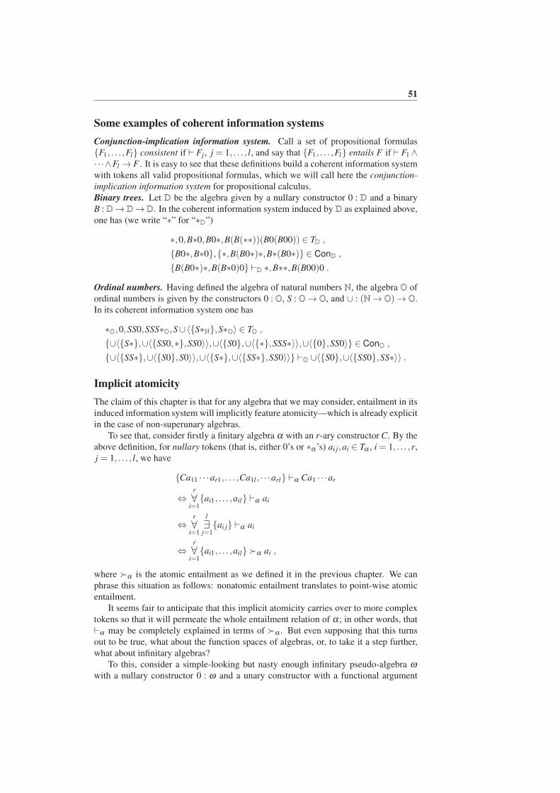
51
Some examples of coherent information systems
Conjunction-implication information system. Call a set of propositional formulas
F1, . . . ,Fl consistent if ⊢ Fj, j = 1, . . . , l, and say that F1, . . . ,Fl entails F if ⊢ F1∧·· ·∧Fl → F . It is easy to see that these definitions build a coherent information system
with tokens all valid propositional formulas, which we will call here the conjunction-
implication information system for propositional calculus.
Binary trees. Let D be the algebra given by a nullary constructor 0 : D and a binary
B :D→D→D. In the coherent information system induced by D as explained above,
one has (we write “∗” for “∗D”)
∗,0,B∗0,B0∗,B(B(∗∗))(B0(B00)) ∈ TD ,
B0∗,B∗0,∗,B(B0∗)∗,B∗(B0∗) ∈ ConD ,
B(B0∗)∗,B(B∗0)0 ⊢D ∗,B∗∗,B(B00)0 .
Ordinal numbers. Having defined the algebra of natural numbers N, the algebra O of
ordinal numbers is given by the constructors 0 : O, S : O→ O, and ∪ : (N→ O)→ O.
In its coherent information system one has
∗O,0,SS0,SSS∗O,S∪〈S∗N,S∗O〉 ∈ TO ,
∪〈S∗,∪〈SS0,∗,SS0〉〉,∪〈S0,∪〈∗,SSS∗〉〉,∪〈0,SS0〉 ∈ ConO ,
∪〈SS∗,∪〈S0,S0〉〉,∪〈S∗,∪〈SS∗,SS0〉〉 ⊢O ∪〈S0,∪〈SS0,SS∗〉〉 .
Implicit atomicity
The claim of this chapter is that for any algebra that we may consider, entailment in its
induced information system will implicitly feature atomicity—which is already explicit
in the case of non-superunary algebras.
To see that, consider firstly a finitary algebra α with an r-ary constructor C. By the
above definition, for nullary tokens (that is, either 0’s or ∗α ’s) ai j,ai ∈ Tα , i = 1, . . . ,r,
j = 1, . . . , l, we have
Ca11 · · ·ar1, . . . ,Ca1l , · · ·arl ⊢α Ca1 · · ·ar
⇔r
∀i=1ai1, . . . ,ail ⊢α ai
⇔r
∀i=1
l
∃j=1ai j ⊢α ai
⇔r
∀i=1ai1, . . . ,ail ≻α ai ,
where ≻α is the atomic entailment as we defined it in the previous chapter. We can
phrase this situation as follows: nonatomic entailment translates to point-wise atomic
entailment.
It seems fair to anticipate that this implicit atomicity carries over to more complex
tokens so that it will permeate the whole entailment relation of α; in other words, that
⊢α may be completely explained in terms of ≻α . But even supposing that this turns
out to be true, what about the function spaces of algebras, or, to take it a step further,
what about infinitary algebras?
To this, consider a simple-looking but nasty enough infinitary pseudo-algebra ωwith a nullary constructor 0 : ω and a unary constructor with a functional argument
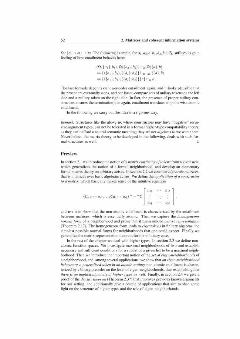
52 2. Matrices and coherent information systems
Ω : (ω → ω)→ ω . The following example, for a1,a2,a,b1,b2,b ∈ Tω suffices to get a
feeling of how entailment behaves here:
Ω〈a1,b1〉,Ω〈a2,b2〉 ⊢ω Ω〈a,b〉
⇔ 〈a1,b1〉,〈a2,b2〉 ⊢ω→ω 〈a,b〉
⇔ 〈a1,b1〉,〈a2,b2〉a ⊢ω b .
The last formula depends on lower-order entailment again, and it looks plausible that
the procedure eventually stops, and one has to compare sets of nullary tokens on the left
side and a nullary token on the right side (in fact, the presence of proper nullary con-
structors ensures the termination); so again, entailment translates to point-wise atomic
entailment.
In the following we carry out this idea in a rigorous way.
Remark. Structures like the above ω , where constructors may have “negative” recur-
sive argument types, can not be tolerated in a formal higher-type computability theory,
as they can’t afford a natural semantic meaning; they are not algebras as we want them.
Nevertheless, the matrix theory to be developed in the following, deals with such for-
mal structures as well.
Preview
In section 2.1 we introduce the notion of a matrix consisting of tokens from a given acis,
which generalizes the notion of a formal neighborhood, and develop an elementary
formal matrix theory on arbitrary acises. In section 2.2 we consider algebraic matrices,
that is, matrices over basic algebraic acises. We define the application of a constructor
to a matrix, which basically makes sense of the intuitive equation
Ca11 · · ·ar1, . . . ,Ca1l · · ·arl “ = ” C
a11 · · · a1l
.... . .
...ar1 · · · arl
,
and use it to show that the non-atomic entailment is characterized by the entailment
between matrices, which is essentially atomic. Then we capture the homogeneous
normal form of a neighborhood and prove that it has a unique matrix representation
(Theorem 2.17). The homogeneous form leads to eigentokens in finitary algebras, the
simplest possible normal forms for neighborhoods that one could expect. Finally we
generalize the matrix representation theorem for the infinitary case.
In the rest of the chapter we deal with higher types. In section 2.3 we define non-
atomic function spaces. We investigate maximal neighborhoods of lists and establish
necessary and sufficient conditions for a sublist of a given list to be a maximal neigh-
borhood. Then we introduce the important notion of the set of eigen-neighborhoods of
a neighborhood, and, among several applications, we show that an eigen-neighborhood
behaves as a generalized token in an atomic setting: non-atomic entailment is charac-
terized by a binary preorder on the level of eigen-neighborhoods, thus establishing that
there is an implicit atomicity at higher types as well. Finally, in section 2.4 we give a
proof of the density theorem (Theorem 2.37) that improves previous known arguments
for our setting, and additionally give a couple of applications that aim to shed some
light on the structure of higher types and the role of eigen-neighborhoods.
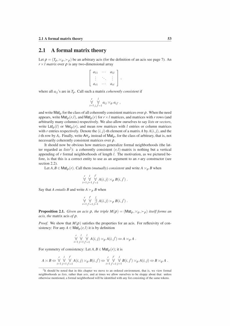
2.1 A formal matrix theory 53
2.1 A formal matrix theory
Let ρ = (Tρ ,≍ρ ,≻ρ) be an arbitrary acis (for the definition of an acis see page 7). An
r× l matrix over ρ is any two-dimensional array
a11 · · · a1l
.... . .
...ar1 · · · arl
,
where all ai j’s are in Tρ . Call such a matrix coherently consistent if
r
∀i=1
l
∀j, j′=1
ai j ≍ρ ai j′ ,
and write Matρ for the class of all coherently consistent matrices over ρ . When the need
appears, write Matρ(r, l), and Matρ(r) for r× l matrices, and matrices with r rows (and
arbitrarily many columns) respectively. We also allow ourselves to say lists or vectors,
write Lstρ(l) or Vecρ(r), and mean row matrices with l entries or column matrices
with r entries respectively. Denote the (i, j)-th element of a matrix A by A(i, j), and the
i-th row by Ai. Finally, write Arrρ instead of Matρ , for the class of arbitrary, that is, not
necessarily coherently consistent matrices over ρ .
It should now be obvious how matrices generalize formal neighborhoods (the lat-
ter regarded as lists2): a coherently consistent (r, l)-matrix is nothing but a vertical
appending of r formal neighborhoods of length l. The motivation, as we pictured be-
fore, is that this is a correct entity to use as an argument to an r-ary constructor (see
section 2.2).
Let A,B ∈Matρ(r). Call them (mutually) consistent and write A≍ρ B when
r
∀i=1
l
∀j=1
l′
∀j′=1
A(i, j)≍ρ B(i, j′) .
Say that A entails B and write A≻ρ B when
r
∀i=1
l′
∀j′=1
l
∃j=1
A(i, j)≻ρ B(i, j′) .
Proposition 2.1. Given an acis ρ , the triple M(ρ) = (Matρ ,≍ρ ,≻ρ) itself forms an
acis, the matrix acis of ρ .
Proof. We show that M(ρ) satisfies the properties for an acis. For reflexivity of con-
sistency: For any A ∈Matρ(r, l) it is by definition
r
∀i=1
l
∀j=1
l
∀j′=1
A(i, j)≍ρ A(i, j′)⇔ A≍ρ A .
For symmetry of consistency: Let A,B ∈Matρ(r); it is
A≍ B⇔r
∀i=1
l
∀j=1
l′
∀j′=1
A(i, j)≍ρ B(i, j′)⇔r
∀i=1
l′
∀j′=1
l
∀j=1
B(i, j′)≍ρ A(i, j)⇔ B≍ρ A .
2It should be noted that in this chapter we move to an ordered environment, that is, we view formal
neighborhoods as lists, rather than sets, and at times we allow ourselves to be sloppy about that: unless
otherwise mentioned, a formal neighborhood will be identified with any list consisting of the same tokens.
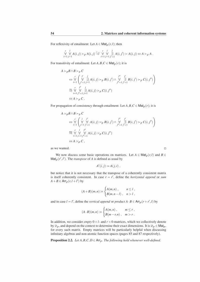
54 2. Matrices and coherent information systems
For reflexivity of entailment: Let A ∈Matρ(r, l); then
r
∀i=1
l
∀j=1
A(i, j)≻ρ A(i, j)j′ ≔ j
⇒r
∀i=1
l
∀j=1
l
∃j′=1
A(i, j′)≻ A(i, j)⇔ A≻ρ A .
For transitivity of entailment: Let A,B,C ∈Matρ(r); it is
A≻ρ B∧B≻ρ C
⇔r
∀i=1
(l′
∀j′=1
l
∃j=1
A(i, j)≻ρ B(i, j′)∧l′′
∀j′′=1
l′
∃j′=1
B(i, j′)≻ρ C(i, j′′)
)
trns⇒
r
∀i=1
l′′
∀j′′=1
l
∃j=1
A(i, j)≻ρ C(i, j′′)
⇔ A≻ρ C .
For propagation of consistency through entailment: Let A,B,C ∈Matρ(r); it is
A≍ρ B∧B≻ρ C
⇔r
∀i=1
(l
∀j=1
l′
∀j′=1
A(i, j)≍ρ B(i, j′)∧l′′
∀j′′=1
l′
∃j′=1
B(i, j′)≻ρ C(i, j′′)
)
prpg
⇒r
∀i=1
l
∀j=1
l′′
∀j′′=1
A(i, j)≍ρ C(i, j′′)
⇔ A≍ρ C ,
as we wanted.
We now discuss some basic operations on matrices. Let A ∈ Matρ(r, l) and B ∈Matρ(r
′, l′). The transpose of A is defined as usual by
At(i, j)≔ A( j, i) ,
but notice that it is not necessary that the transpose of a coherently consistent matrix
is itself coherently consistent. In case r = r′, define the horizontal append or sum
A+B ∈ Arrρ(r, l + l′) by
(A+B)(m,n)≔
A(m,n) , n≤ l ,
B(m,n− l) , n > l ,
and in case l = l′, define the vertical append or product A ·B ∈ Arrρ(r+ r′, l) by
(A ·B)(m,n)≔
A(m,n) , m≤ r ,
B(m− r,n) , m > r .
In addition, we consider empty 0× l- and r×0-matrices, which we collectively denote
by ∅ρ , and depend on the context to determine their exact dimensions. It is ∅ρ ∈Matρ ,
for every such matrix. Empty matrices will be particularly helpful when discussing
infinitary algebras and non-atomic function spaces (pages 85 and 87 respectively).
Proposition 2.2. Let A,B,C,D ∈ Arrρ . The following hold whenever well-defined.
2.1 A formal matrix theory 55
1. If A,B ∈ Matρ then A ·B ∈ Matρ , and if furthermore A ≍ρ B it is also A+B ∈Matρ .
2. Both append operations are monotone, that is,
A≻ρ A′∧B≻ B′→ AA′ ≻ρ BB′ ,
where is either + or ·.
3. It is A≍ρ ∅ and A≻ρ ∅, for every A ∈Matρ .
4. The following equations hold:
(A+B)+C = A+(B+C) ,
A+∅= A = ∅+A ,
(A ·B) ·C = A · (B ·C) ,
A ·∅= A = ∅ ·A ,
(A+B) · (C+D) = (A ·C)+(B ·D) ,
A ·B =(
At +Bt)t
.
With the convention of writing a for a one-element matrix [a], Proposition 2.2
yields two alternative notations for an arbitrary matrix A ∈ Arrρ(r, l), an additive-
multiplicative and a multiplicative-additive (or sigma-pi and pi-sigma respectively):
A =l
∑j=1
r
∏i=1
A(i, j) =r
∏i=1
l
∑j=1
A(i, j) ,
both of which will later prove useful.
Mixed matrices
In anticipation of both infinitary algebras (where functional recursive arguments ap-
pear) and parametric algebras, we also introduce a kind of generalized matrices, where
each row might draw from a different acis. By a mixed matrix A of dimensions
(ρ1, . . . ,ρr)× l we will mean a two-dimensional array
a11 · · · a1l
.... . .
...ar1 · · · arl
,
where, for each i = 1, . . . ,r, all ai j’s are in Tρi; we write A ∈ Arr(ρ1, . . . ,ρr, l).
All notions pertaining to simple matrices, like coherent consistency, mutual consis-
tency, and entailment, as well as the structural operations and all relevant facts, carry
over to mixed matrices without any problems—to convince oneself, one should notice
how all definitions work row-wise, as the following observation ensures.
Proposition 2.3. Let ρ1, . . . ,ρr be acises. It is
Arr(ρ1, . . . ,ρr, l)≃ Arrρ1(1, l)×·· ·×Arrρr(1, l) ,
for all l > 0.
56 2. Matrices and coherent information systems
Proof. A matrix A ∈ Arr(ρ1, . . . ,ρr, l) can be mapped to the r-tuple (A1, . . . ,Ar) of
its rows; conversely, given an r-tuple (A1, . . . ,Ar), with Ai ∈ Arrρi(1, l) for every i =
1, . . . ,r, we have ∏ri=1 Ai ∈Arr(ρ1, . . . ,ρr, l). The mappings are clearly an isomorphism
pair.
Atomic function spaces I
We already have enough to go on with the main course, which is, matrices over alge-
bras, or algebraic matrices (section 2.2). Still, we linger on the formal level for the
remainder of this section, and examine the case of atomic function spaces. This, apart
from making the formal exposition more complete, will also help obtain a better un-
derstanding of the behavior of matrices, and also, allow to take a glimpse at interesting
structures that arise on the way (see nbr-acises, page 100), and try out ideas that will
play a crucial role in the case of the algebraic matrices, and their non-atomic function
spaces (see test matrices, page 58).
We will readily see that the generalization of the above to atomic function spaces is
not so direct; here logic plays a dominant role, which takes some effort to be translated
into matrix terms. Let us begin in the obvious and natural way. An r× l matrix over
ρ → σ is any two-dimensional array
〈U11,a11〉 · · · 〈U1l ,a1l〉...
. . ....
〈Ur1,ar1〉 · · · 〈Url ,arl〉
,
where all Ui j’s are in Conρ and ai j’s are in Tσ . We denote the class of all such arrays
by Arrρ→σ . Obstacles appear already when one considers the subclass of coherently
consistent matrices over ρ → σ , and further the notions of mutual consistency and
entailment. For the latter two we have the following. Let
A≔
〈U11,a11〉 · · · 〈U1l ,a1l〉...
. . ....
〈Ur1,ar1〉 · · · 〈Url ,arl〉
and B≔
〈V11,b11〉 · · · 〈V1l′ ,b1l′〉...
. . ....
〈Vr1,br1〉 · · · 〈Vrl′ ,brl′〉
.
The matrices A,B ∈Matρ(r) should be (mutually) consistent when
A≍ρ→σ B⇔r
∀i=1
l
∀j=1
l′
∀j′=1
A(i, j)≍ρ→σ B(i, j′)
⇔r
∀i=1
l
∀j=1
l′
∀j′=1〈Ui j,ai j〉 ≍ρ→σ 〈Vi j′ ,bi j′〉
⇔r
∀i=1
l
∀j=1
l′
∀j′=1
(
Ui j ≍ρ Vi j′ → ai j ≍σ bi j′)
—note that coherent consistency of a matrix is a special case of mutual consistency of
2.1 A formal matrix theory 57
two matrices: it is A ∈Mat if and only if A≍ A. Further, A should entail B when
A≻ρ→σ B⇔r
∀i=1
l′
∀j′=1
l
∃j=1
A(i, j)≻ρ→σ B(i, j′)
⇔r
∀i=1
l′
∀j′=1
l
∃j=1〈Ui j,ai j〉 ≻ρ→σ 〈Vi j′ ,bi j′〉
⇔r
∀i=1
l′
∀j′=1
l
∃j=1
(
Vi j′ ≻ρ Ui j ∧ai j ≻σ bi j′)
.
Clearly, it is not trivial to formulate the above formulas in matrix terms. In order to
do that we will use some extra tools, in particular, appropriate versions of “adjacency
matrices” for consistency and entailment.
Test matrices
Let I = 1, . . . ,r, J = 1, . . . , l, J′ = 1, . . . , l′, and I′ = 1, . . . ,rl. Consider the
blocking map b : I× J× J′ → I′× J′, and the unblocking maps u0 : I′× J′ → I, u1 :
I′× J′→ J, and u0 : I′× J′→ J′, that are defined by
b(i, j, j′)≔(
(i−1)l + j, j′)
,
u0(i′, j′)≔ (i′−1)r l +1 ,
u1(i′, j′)≔ ((i′−1) mod l)+1 ,
u2(i′, j′)≔ j′ ,
where mrn and m mod n are the integer quotient and the remainder of the division of
m by n, and i ∈ I, j ∈ J, j′ ∈ J′, i′ ∈ I′.
Proposition 2.4. The mappings b : I× J× J′→ I′× J′ and u≔ (u0,u1,u2) : I′× J′→I× J× J′ form a bijection pair, called block coding (of indices).
Proof. One has to show that
∀i∈I, j∈J, j′∈J′
u(b(i, j, j′)) =(
i, j, j′)
,
∀i′∈I′, j′∈J′
b(u(i′, j′)) =(
i′, j′)
.
For the first property, let i ∈ I, j ∈ J, and j′ ∈ J′. It is
u(b(i, j, j′)) = u(
(i−1)l + j, j′)
=(
u0
(
(i−1)l + j, j′)
,u1
(
(i−1)l + j, j′)
,u2
(
(i−1)l + j, j′))
,
with
u0
(
(i−1)l + j, j′)
= ((i−1)l + j−1)r l +1 = i ,
u1
(
(i−1)l + j, j′)
= ((i−1)l + j−1) mod l +1 = j ,
u2
(
(i−1)l + j, j′)
= j′ ,
so u(b(i, j, j′)) = (i, j, j′).
58 2. Matrices and coherent information systems
For the converse property, let i′ ∈ I′ and j′ ∈ J′. Then
b(u(i′, j′)) = b(
u0(i′, j′),u1(i
′, j′),u2(i′, j′)
)
=(
(u0(i′, j′)−1)l +u1(i
′, j′),u2(i′, j′)
)
=(
((i′−1)r l)l +(i′−1) mod l +1, j′)
= (i′, j′) ,
where for the last step we used the identity
(mrn)n+m mod n = m ,
for m,n ∈ N.
If A ∈ Arrρ(r, l) and B ∈ Arrρ(r, l′) are two arbitrary matrices, we can use this block
coding to form a block matrix with r blocks; each block will have l rows and l′ columns,
so that it may serve as a “comparison table” between (positions of) elements of A and
B in their respective row; we understand b(i, j, j′) as “the position ( j, j′) in the i-th
block”.
In particular we need such comparison tables to test consistency and entailment
between elements of the two matrices in the same row. For an arbitrary acis ρ define
the mappings?≍ρ ,
?≻ρ : Arrρ(r, l)×Arrρ(r, l
′)→ ArrB(rl, l′) by
A?≍ρ B(i′, j′)≔
tt , A(u01(i′, j′))≍ρ B(u02(i
′, j′)) ,
∗B , otherwise ,
A?≻ρ B(i′, j′)≔
tt , A(u01(i′, j′))≻ρ B(u02(i
′, j′)) ,
∗B , otherwise ,
where u01 ≔ (u0,u1) and u02 ≔ (u0,u2). We call A?≍ρ B and A
?≻ρ B the consistency
and entailment test matrix respectively of A and B.
Proposition 2.5. Let A ∈ Arrρ(r, l), B ∈ Arrρ(r, l′), C ∈ Arrρ(r, l
′′), and let i = 1, . . . ,r,
j = 1, . . . , l, j′ = 1, . . . , l′, j′′ = 1, . . . , l′′.
1. It is A≍ρ B if and only if their consistency test matrix is the true matrix, that is,
∀i∀j∀j′
A?≍ρ B(b(i, j, j′)) = tt .
2. It is A?≍ρ A(b(i, j, j)) = tt, for all i, j.
3. It is A?≍ρ B(b(i, j, j′)) = B
?≍ρ A(b(i, j′, j)), for all i, j, j′.
4. It is A ≻ρ B if and only if their entailment test matrix consists of blocks with
non-blank columns, that is,
∀i∀j′∃j
A?≻ρ B(b(i, j, j′)) = tt .
5. It is A?≻ρ A(b(i, j, j)) = tt, for all i, j.
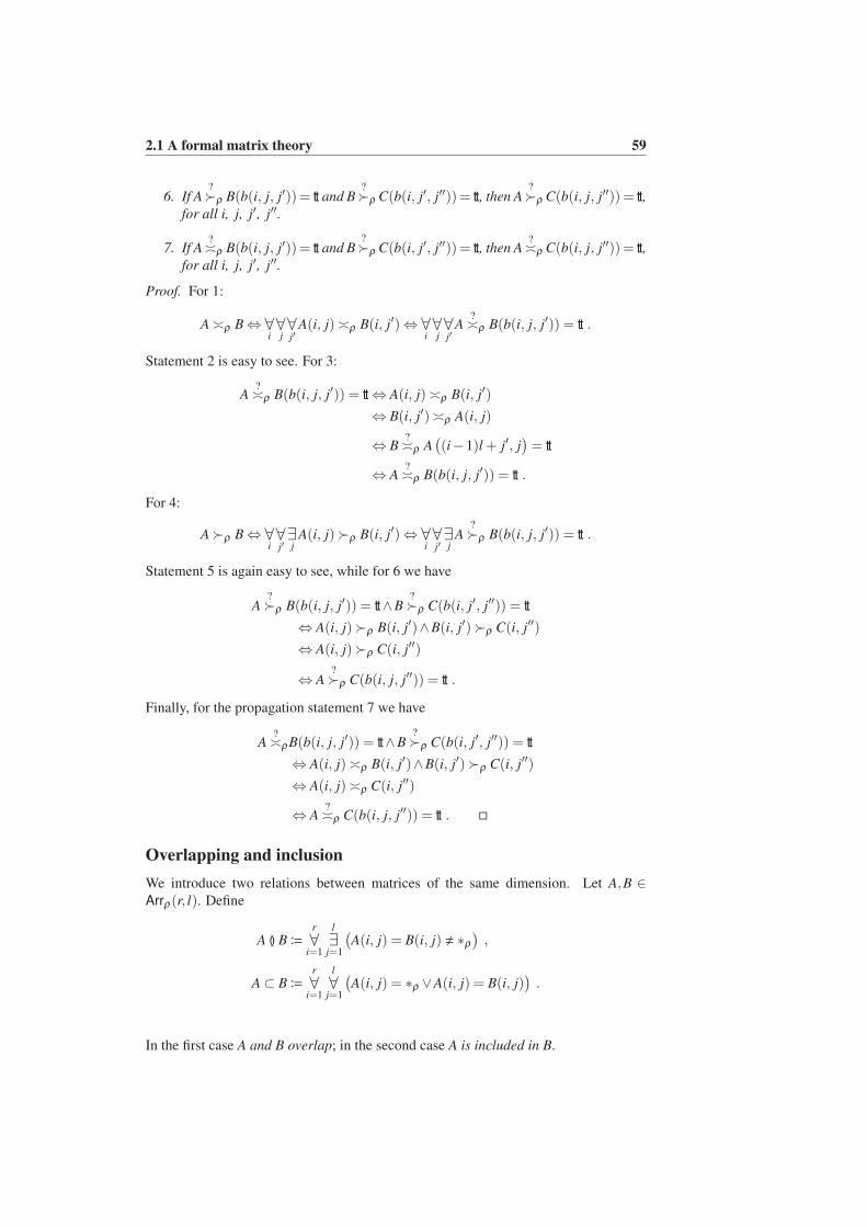
2.1 A formal matrix theory 59
6. If A?≻ρ B(b(i, j, j′))= tt and B
?≻ρ C(b(i, j′, j′′))= tt, then A
?≻ρ C(b(i, j, j′′))= tt,
for all i, j, j′, j′′.
7. If A?≍ρ B(b(i, j, j′))= tt and B
?≻ρ C(b(i, j′, j′′))= tt, then A
?≍ρ C(b(i, j, j′′))= tt,
for all i, j, j′, j′′.
Proof. For 1:
A≍ρ B⇔ ∀i∀j∀j′
A(i, j)≍ρ B(i, j′)⇔ ∀i∀j∀j′
A?≍ρ B(b(i, j, j′)) = tt .
Statement 2 is easy to see. For 3:
A?≍ρ B(b(i, j, j′)) = tt⇔ A(i, j)≍ρ B(i, j′)
⇔ B(i, j′)≍ρ A(i, j)
⇔ B?≍ρ A
(
(i−1)l + j′, j)
= tt
⇔ A?≍ρ B(b(i, j, j′)) = tt .
For 4:
A≻ρ B⇔ ∀i∀j′∃j
A(i, j)≻ρ B(i, j′)⇔ ∀i∀j′∃j
A?≻ρ B(b(i, j, j′)) = tt .
Statement 5 is again easy to see, while for 6 we have
A?≻ρ B(b(i, j, j′)) = tt∧B
?≻ρ C(b(i, j′, j′′)) = tt
⇔ A(i, j)≻ρ B(i, j′)∧B(i, j′)≻ρ C(i, j′′)
⇔ A(i, j)≻ρ C(i, j′′)
⇔ A?≻ρ C(b(i, j, j′′)) = tt .
Finally, for the propagation statement 7 we have
A?≍ρ B(b(i, j, j′)) = tt∧B
?≻ρ C(b(i, j′, j′′)) = tt
⇔ A(i, j)≍ρ B(i, j′)∧B(i, j′)≻ρ C(i, j′′)
⇔ A(i, j)≍ρ C(i, j′′)
⇔ A?≍ρ C(b(i, j, j′′)) = tt .
Overlapping and inclusion
We introduce two relations between matrices of the same dimension. Let A,B ∈Arrρ(r, l). Define
A ≬ B≔r
∀i=1
l
∃j=1
(
A(i, j) = B(i, j) , ∗ρ
)
,
A⊂ B≔r
∀i=1
l
∀j=1
(
A(i, j) = ∗ρ ∨A(i, j) = B(i, j))
.
In the first case A and B overlap; in the second case A is included in B.
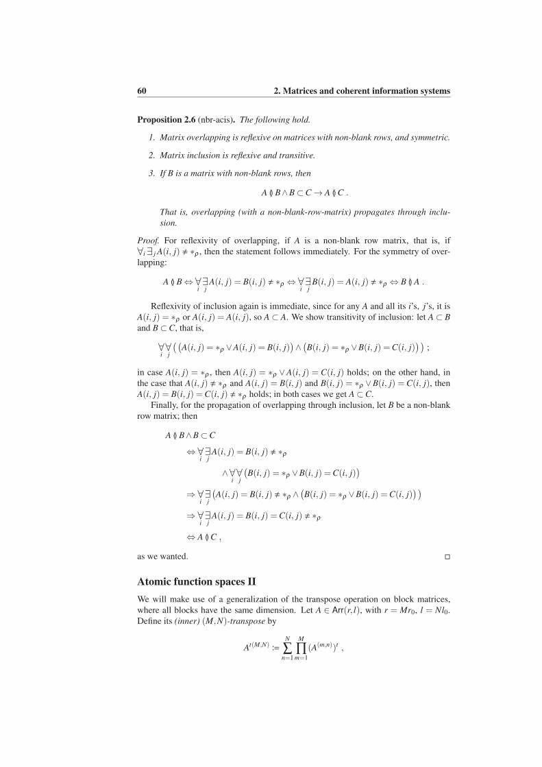
60 2. Matrices and coherent information systems
Proposition 2.6 (nbr-acis). The following hold.
1. Matrix overlapping is reflexive on matrices with non-blank rows, and symmetric.
2. Matrix inclusion is reflexive and transitive.
3. If B is a matrix with non-blank rows, then
A ≬ B∧B⊂C→ A ≬C .
That is, overlapping (with a non-blank-row-matrix) propagates through inclu-
sion.
Proof. For reflexivity of overlapping, if A is a non-blank row matrix, that is, if
∀i∃ j A(i, j) , ∗ρ , then the statement follows immediately. For the symmetry of over-
lapping:
A ≬ B⇔ ∀i∃j
A(i, j) = B(i, j) , ∗ρ ⇔ ∀i∃j
B(i, j) = A(i, j) , ∗ρ ⇔ B ≬ A .
Reflexivity of inclusion again is immediate, since for any A and all its i’s, j’s, it is
A(i, j) = ∗ρ or A(i, j) = A(i, j), so A⊂ A. We show transitivity of inclusion: let A⊂ B
and B⊂C, that is,
∀i∀j
((
A(i, j) = ∗ρ ∨A(i, j) = B(i, j))
∧(
B(i, j) = ∗ρ ∨B(i, j) =C(i, j)))
;
in case A(i, j) = ∗ρ , then A(i, j) = ∗ρ ∨A(i, j) = C(i, j) holds; on the other hand, in
the case that A(i, j) , ∗ρ and A(i, j) = B(i, j) and B(i, j) = ∗ρ ∨B(i, j) = C(i, j), then
A(i, j) = B(i, j) =C(i, j) , ∗ρ holds; in both cases we get A⊂C.
Finally, for the propagation of overlapping through inclusion, let B be a non-blank
row matrix; then
A ≬ B∧B⊂C
⇔ ∀i∃j
A(i, j) = B(i, j) , ∗ρ
∧∀i∀j
(
B(i, j) = ∗ρ ∨B(i, j) =C(i, j))
⇒ ∀i∃j
(
A(i, j) = B(i, j) , ∗ρ ∧(
B(i, j) = ∗ρ ∨B(i, j) =C(i, j)))
⇒ ∀i∃j
A(i, j) = B(i, j) =C(i, j) , ∗ρ
⇔ A ≬C ,
as we wanted.
Atomic function spaces II
We will make use of a generalization of the transpose operation on block matrices,
where all blocks have the same dimension. Let A ∈ Arr(r, l), with r = Mr0, l = Nl0.
Define its (inner) (M,N)-transpose by
At(M,N)≔
N
∑n=1
M
∏m=1
(A(m,n))t ,
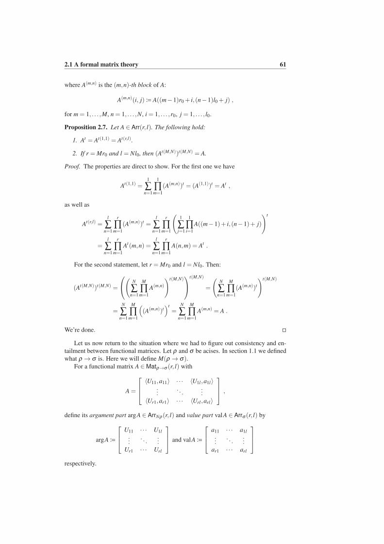
2.1 A formal matrix theory 61
where A(m,n) is the (m,n)-th block of A:
A(m,n)(i, j)≔ A((m−1)r0 + i,(n−1)l0 + j) ,
for m = 1, . . . ,M, n = 1, . . . ,N, i = 1, . . . ,r0, j = 1, . . . , l0.
Proposition 2.7. Let A ∈ Arr(r, l). The following hold:
1. At = At(1,1) = At(r,l).
2. If r = Mr0 and l = Nl0, then (At(M,N))t(M,N) = A.
Proof. The properties are direct to show. For the first one we have
At(1,1) =1
∑n=1
1
∏m=1
(A(m,n))t = (A(1,1))t = At ,
as well as
At(r,l) =l
∑n=1
r
∏m=1
(A(m,n))t =l
∑n=1
r
∏m=1
(1
∑j=1
1
∏i=1
A((m−1)+ i,(n−1)+ j)
)t
=l
∑n=1
r
∏m=1
At(m,n) =l
∑n=1
r
∏m=1
A(n,m) = At .
For the second statement, let r = Mr0 and l = Nl0. Then:
(At(M,N))t(M,N) =
(N
∑n=1
M
∏m=1
A(m,n)
)t(M,N)
t(M,N)
=
(N
∑n=1
M
∏m=1
(A(m,n))t
)t(M,N)
=N
∑n=1
M
∏m=1
(
(A(m,n))t)t
=N
∑n=1
M
∏m=1
A(m,n) = A .
We’re done.
Let us now return to the situation where we had to figure out consistency and en-
tailment between functional matrices. Let ρ and σ be acises. In section 1.1 we defined
what ρ → σ is. Here we will define M(ρ → σ).For a functional matrix A ∈Matρ→σ (r, l) with
A =
〈U11,a11〉 · · · 〈U1l ,a1l〉...
. . ....
〈Ur1,ar1〉 · · · 〈Url ,arl〉
,
define its argument part argA ∈ ArrNρ(r, l) and value part valA ∈ Arrσ (r, l) by
argA≔
U11 · · · U1l
.... . .
...Ur1 · · · Url
and valA≔
a11 · · · a1l
.... . .
...ar1 · · · arl
respectively.
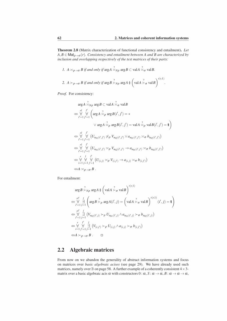
62 2. Matrices and coherent information systems
Theorem 2.8 (Matrix characterization of functional consistency and entailment). Let
A,B ∈Matρ→σ (r). Consistency and entailment between A and B are characterized by
inclusion and overlapping respectively of the test matrices of their parts:
1. A≍ρ→σ B if and only if argA?≍Nρ argB⊂ valA
?≍σ valB.
2. A≻ρ→σ B if and only if argB?≻Nρ argA ≬
(
valA?≻σ valB
)t(r,1)
.
Proof. For consistency:
argA?≍Nρ argB⊂ valA
?≍σ valB
⇔rl
∀i′=1
l′
∀j′=1
(
argA?≍ρ argB(i′, j′) = ∗
∨ argA?≍ρ argB(i′, j′) = valA
?≍ρ valB(i′, j′) = tt
)
⇔rl
∀i′=1
l′
∀j′=1
(
Uu01(i′, j′) 6≍ρ Vu02(i′, j′)∨au01(i′, j′) ≍σ bu02(i′, j′)
)
⇔rl
∀i′=1
l′
∀j′=1
(
Uu01(i′, j′) ≍ρ Vu02(i′, j′)→ au01(i′, j′) ≍σ bu02(i′, j′)
)
⇔r
∀i=1
l
∀j=1
l′
∀j′=1
(
U(i, j) ≍ρ V(i, j′)→ a(i, j) ≍σ b(i, j′))
⇔A≍ρ→σ B .
For entailment:
argB?≻Nρ argA ≬
(
valA?≻σ valB
)t(r,1)
⇔rl′
∀i′=1
l
∃j=1
(
argB?≻ρ argA(i′, j) =
(
valA?≻σ valB
)t(r,1)
(i′, j) = tt
)
⇔rl′
∀i′=1
l
∃j=1
(
Vu02(i′, j) ≻ρ Uu01(i′, j)∧au01(i′, j) ≻σ bu02(i′, j)
)
⇔r
∀i=1
l′
∀j′=1
l
∃j=1
(
V(i, j′) ≻ρ U(i, j)∧a(i, j) ≻σ b(i, j′))
⇔A≻ρ→σ B .
2.2 Algebraic matrices
From now on we abandon the generality of abstract information systems and focus
on matrices over basic algebraic acises (see page 29). We have already used such
matrices, namely overB on page 58. A further example of a coherently consistent 4×3-
matrix over a basic algebraic acis α with constructors 0 : α , S : α →α , B : α →α →α ,
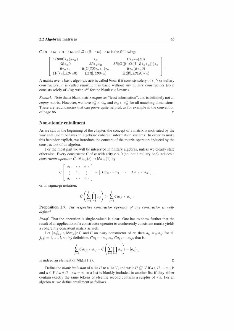
2.2 Algebraic matrices 63
C : α → α → α → α , and Ω : (B→ α)→ α is the following:
C(B00)∗α(S∗α) ∗α C∗α∗α(S0)SB∗α 0 SB∗α∗α SB(Ω〈[tt],Ω〈[ff],B∗α∗α〉〉)∗α
B∗α∗α B(C(S0)∗α∗α)∗α B∗α(B∗α 0)Ω〈[∗B],SB∗α 0〉 Ω〈[tt],SB0∗α〉 Ω〈[ff],SB(S0)∗α〉
.
A matrix over a basic algebraic acis is called basic if it consists solely of ∗α ’s or nullary
constructors; it is called blank if it is basic without any nullary constructors (so it
consists solely of ∗’s); write ∗r,l for the blank r× l-matrix.
Remark. Note that a blank matrix expresses “least information”, and is definitely not an
empty matrix. However, we have ∗r,lα ≻ ∅α and ∅α ≻ ∗
r,lα for all matching dimensions.
These are redundancies that can prove quite helpful, as for example in the convention
of page 86.
Non-atomic entailment
As we saw in the beginning of the chapter, the concept of a matrix is motivated by the
way entailment behaves in algebraic coherent information systems. In order to make
this behavior explicit, we introduce the concept of the matrix operators induced by the
constructors of an algebra.
For the most part we will be interested in finitary algebras, unless we clearly state
otherwise. Every constructor C of α with arity r > 0 (so, not a nullary one) induces a
constructor operator C : Matα(r)→Matα(1) by
C
a11 · · · a1l
.... . .
...ar1 · · · arl
≔
[Ca11 · · ·ar1 · · · Ca1l · · ·arl
],
or, in sigma-pi notation:
C
(l
∑j=1
r
∏i=1
ai j
)
≔
l
∑j=1
Ca1 j · · ·ar j .
Proposition 2.9. The respective constructor operator of any constructor is well-
defined.
Proof. That the operation is single-valued is clear. One has to show further that the
result of an application of a constructor operator to a coherently consistent matrix yields
a coherently consistent matrix as well.
Let [ai j]i, j ∈ Matα(r, l) and C an r-ary constructor of α; then ai j ≍α ai j′ for all
j, j′ = 1, . . . , l, so, by definition, Ca1 j · · ·ar j ≍α Ca1 j′ · · ·ar j′ , that is,
l
∑j=1
Ca1 j · · ·ar j = C
(l
∑j=1
r
∏i=1
ai j
)
= [ai j]i, j
is indeed an element of Matα(1, l).
Define the blank inclusion of a list U to a list V , and write U ⊆∗ V if a∈U → a∈V
and a ∈ V ∧ a <U → a = ∗; so a list is blankly included in another list if they either
contain exactly the same tokens or else the second contains a surplus of ∗’s. For an
algebra α , we define entailment as follows.
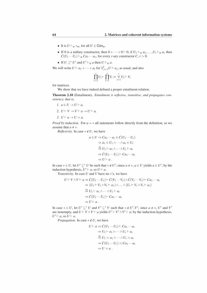
64 2. Matrices and coherent information systems
• It is U ⊢α ∗α , for all U ∈ Conα .
• If 0 is a nullary constructor, then 0+ · · ·+ 0 ⊢ 0; if U1 ⊢α a1, . . . ,Ur ⊢α ar then
C(U1 · · ·Ur) ⊢α Ca1 · · ·ar, for every r-ary constructor C, r > 0.
• If U ⊇∗ U ′ and U ′ ⊢α a then U ⊢α a.
We will write U ⊢ a1 + · · ·+al for ∀lj=1 U ⊢ a j, as usual, and also
r
∏i=1
Ui ⊢r
∏i=1
Vi ≔
r
∀i=1
Ui ⊢Vi
for matrices.
We show that we have indeed defined a proper entailment relation.
Theorem 2.10 (Entailment). Entailment is reflexive, transitive, and propagates con-
sistency, that is,
1. a ∈U →U ⊢ a,
2. U ⊢V →V ⊢ a→U ⊢ a,
3. U ⊢ a→U ≍ a.
Proof by induction. For a = ∗ all statements follow directly from the definition, so we
assume that a , ∗.Reflexivity. In case ∗ <U , we have
a ∈U ⇒Ca1 · · ·ar ∈ C(U1 · · ·Ur)
⇒ a1 ∈U1∧·· ·∧ar ∈Ur
IH⇒U1 ⊢ a1∧·· ·∧Ur ⊢ ar
⇒ C(U1 · · ·Ur) ⊢Ca1 · · ·ar
⇒U ⊢ a .
In case ∗ ∈U , let U ′ ⊆∗ U be such that ∗ <U ′; since a , ∗, a ∈U yields a ∈U ′; by the
induction hypothesis, U ′ ⊢ a, so U ⊢ a.
Transitivity. In case U and V have no ∗’s, we have
U ⊢V ∧V ⊢ a⇒ C(U1 · · ·Ur) ⊢ C(V1 · · ·Vr)∧C(V1 · · ·Vr) ⊢Ca1 · · ·ar
⇒ (U1 ⊢V1∧V1 ⊢ a1)∧ . . .∧ (Ur ⊢Vr ∧Vr ⊢ ar)IH⇒U1 ⊢ a1∧·· ·∧Ur ⊢ ar
⇒ C(U1 · · ·Ur) ⊢Ca1 · · ·ar
⇒U ⊢ a .
In case ∗ ∈U , let U ′ ⊆∗ U and V ′ ⊆∗ V such that ∗ <U ′,V ′; since a , ∗, U ′ and V ′
are nonempty, and U ⊢V ∧V ⊢ a yields U ′ ⊢V ′∧V ′ ⊢ a; by the induction hypothesis,
U ′ ⊢ a, so U ⊢ a.
Propagation. In case ∗ <U , we have
U ⊢ a⇒ C(U1 · · ·Ur) ⊢Ca1 · · ·ar
⇒U1 ⊢ a1∧·· ·∧Ur ⊢ ar
IH⇒U1 ≍ a1∧·· ·∧Ur ≍ ar
⇒ C(U1 · · ·Ur)≍Ca1 · · ·ar
⇒U ≍ a .
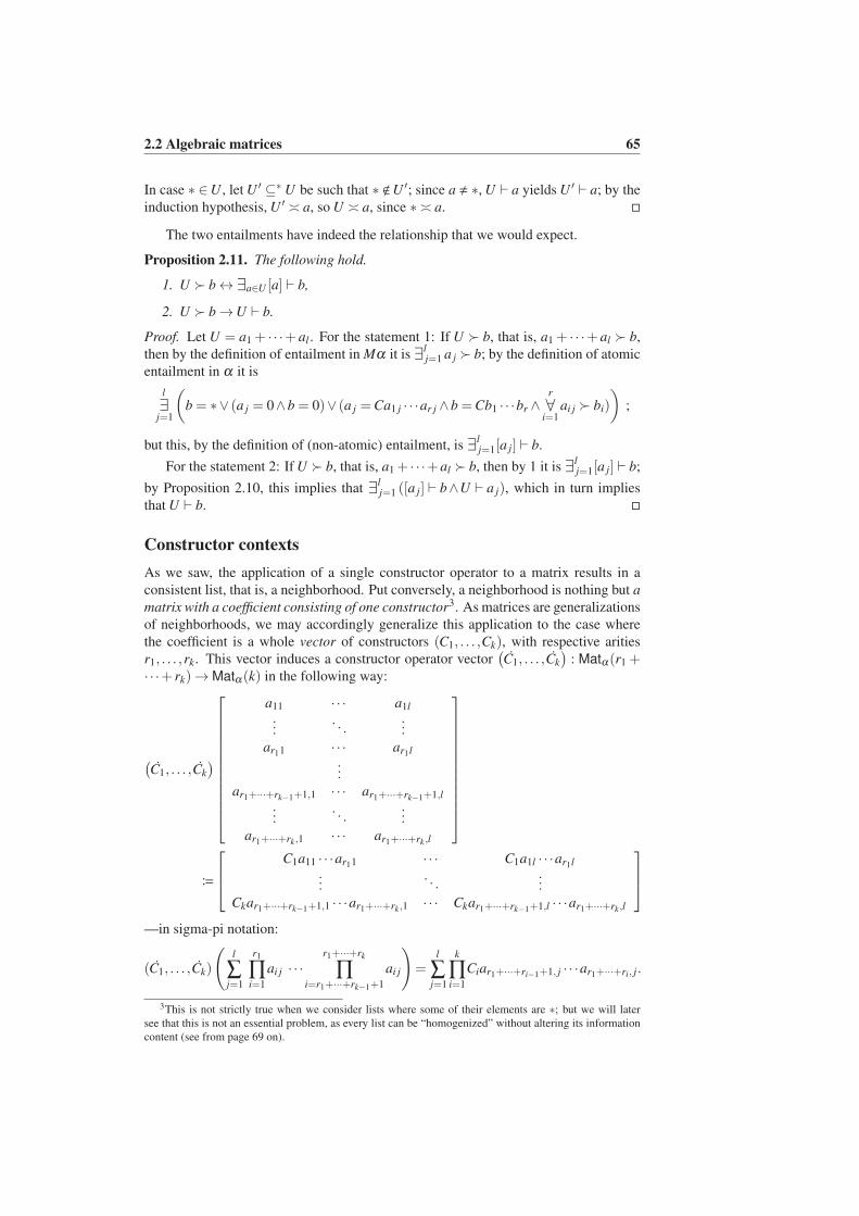
2.2 Algebraic matrices 65
In case ∗ ∈U , let U ′ ⊆∗ U be such that ∗ <U ′; since a , ∗, U ⊢ a yields U ′ ⊢ a; by the
induction hypothesis, U ′ ≍ a, so U ≍ a, since ∗ ≍ a.
The two entailments have indeed the relationship that we would expect.
Proposition 2.11. The following hold.
1. U ≻ b↔ ∃a∈U [a] ⊢ b,
2. U ≻ b→U ⊢ b.
Proof. Let U = a1 + · · ·+al . For the statement 1: If U ≻ b, that is, a1 + · · ·+al ≻ b,
then by the definition of entailment in Mα it is ∃lj=1 a j ≻ b; by the definition of atomic
entailment in α it is
l
∃j=1
(
b = ∗∨ (a j = 0∧b = 0)∨ (a j =Ca1 j · · ·ar j ∧b =Cb1 · · ·br ∧r
∀i=1
ai j ≻ bi)
)
;
but this, by the definition of (non-atomic) entailment, is ∃lj=1[a j] ⊢ b.
For the statement 2: If U ≻ b, that is, a1 + · · ·+al ≻ b, then by 1 it is ∃lj=1[a j] ⊢ b;
by Proposition 2.10, this implies that ∃lj=1 ([a j] ⊢ b∧U ⊢ a j), which in turn implies
that U ⊢ b.
Constructor contexts
As we saw, the application of a single constructor operator to a matrix results in a
consistent list, that is, a neighborhood. Put conversely, a neighborhood is nothing but a
matrix with a coefficient consisting of one constructor3. As matrices are generalizations
of neighborhoods, we may accordingly generalize this application to the case where
the coefficient is a whole vector of constructors (C1, . . . ,Ck), with respective arities
r1, . . . ,rk. This vector induces a constructor operator vector(
C1, . . . ,Ck
)
: Matα(r1 +· · ·+ rk)→Matα(k) in the following way:
(
C1, . . . ,Ck
)
a11 · · · a1l
.... . .
...ar11 · · · ar1l
...ar1+···+rk−1+1,1 · · · ar1+···+rk−1+1,l
.... . .
...ar1+···+rk,1 · · · ar1+···+rk,l
≔
C1a11 · · ·ar11 · · · C1a1l · · ·ar1l
.... . .
...Ckar1+···+rk−1+1,1 · · ·ar1+···+rk,1 · · · Ckar1+···+rk−1+1,l · · ·ar1+···+rk,l
—in sigma-pi notation:
(C1, . . . ,Ck)
(
l
∑j=1
r1
∏i=1
ai j · · ·r1+···+rk
∏i=r1+···+rk−1+1
ai j
)
=l
∑j=1
k
∏i=1
Ciar1+···+ri−1+1, j · · ·ar1+···+ri, j.
3This is not strictly true when we consider lists where some of their elements are ∗; but we will later
see that this is not an essential problem, as every list can be “homogenized” without altering its information
content (see from page 69 on).
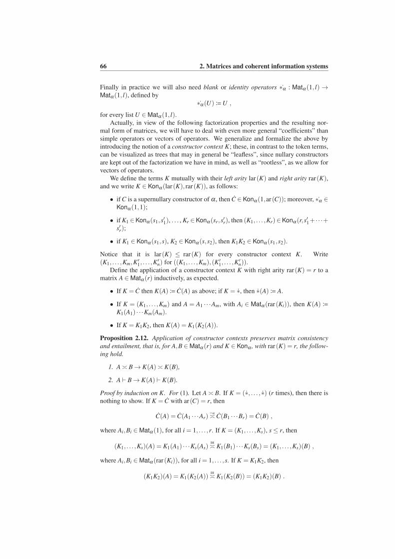
66 2. Matrices and coherent information systems
Finally in practice we will also need blank or identity operators ∗α : Matα(1, l)→Matα(1, l), defined by
∗α(U)≔U ,
for every list U ∈Matα(1, l).Actually, in view of the following factorization properties and the resulting nor-
mal form of matrices, we will have to deal with even more general “coefficients” than
simple operators or vectors of operators. We generalize and formalize the above by
introducing the notion of a constructor context K; these, in contrast to the token terms,
can be visualized as trees that may in general be “leafless”, since nullary constructors
are kept out of the factorization we have in mind, as well as “rootless”, as we allow for
vectors of operators.
We define the terms K mutually with their left arity lar(K) and right arity rar(K),and we write K ∈ Konα(lar(K), rar(K)), as follows:
• if C is a supernullary constructor of α , then C ∈ Konα(1,ar(C)); moreover, ∗α ∈Konα(1,1);
• if K1 ∈Konα(s1,s′1), . . . , Kr ∈Konα(sr,s
′r), then (K1, . . . ,Kr)∈Konα(r,s
′1+ · · ·+
s′r);
• if K1 ∈ Konα(s1,s), K2 ∈ Konα(s,s2), then K1K2 ∈ Konα(s1,s2).
Notice that it is lar(K) ≤ rar(K) for every constructor context K. Write
(K1, . . . ,Km,K′1, . . . ,K
′n) for ((K1, . . . ,Km),(K
′1, . . . ,K
′n)).
Define the application of a constructor context K with right arity rar(K) = r to a
matrix A ∈Matα(r) inductively, as expected.
• If K = C then K(A)≔ C(A) as above; if K = ∗, then ∗(A)≔ A.
• If K = (K1, . . . ,Km) and A = A1 · · ·Am, with Ai ∈ Matα(rar(Ki)), then K(A) ≔K1(A1) · · ·Km(Am).
• If K = K1K2, then K(A) = K1(K2(A)).
Proposition 2.12. Application of constructor contexts preserves matrix consistency
and entailment, that is, for A,B ∈Matα(r) and K ∈ Konα , with rar(K) = r, the follow-
ing hold.
1. A≍ B→ K(A)≍ K(B),
2. A ⊢ B→ K(A) ⊢ K(B).
Proof by induction on K. For (1). Let A ≍ B. If K = (∗, . . . , ∗) (r times), then there is
nothing to show. If K = C with ar(C) = r, then
C(A) = C(A1 · · ·Ar)≍α≍ C(B1 · · ·Br) = C(B) ,
where Ai,Bi ∈Matα(1), for all i = 1, . . . ,r. If K = (K1, . . . ,Ks), s≤ r, then
(K1, . . . ,Ks)(A) = K1(A1) · · ·Ks(As)IH
≍ K1(B1) · · ·Ks(Bs) = (K1, . . . ,Ks)(B) ,
where Ai,Bi ∈Matα(rar(Ki)), for all i = 1, . . . ,s. If K = K1K2, then
(K1K2)(A) = K1(K2(A))IH
≍ K1(K2(B)) = (K1K2)(B) .
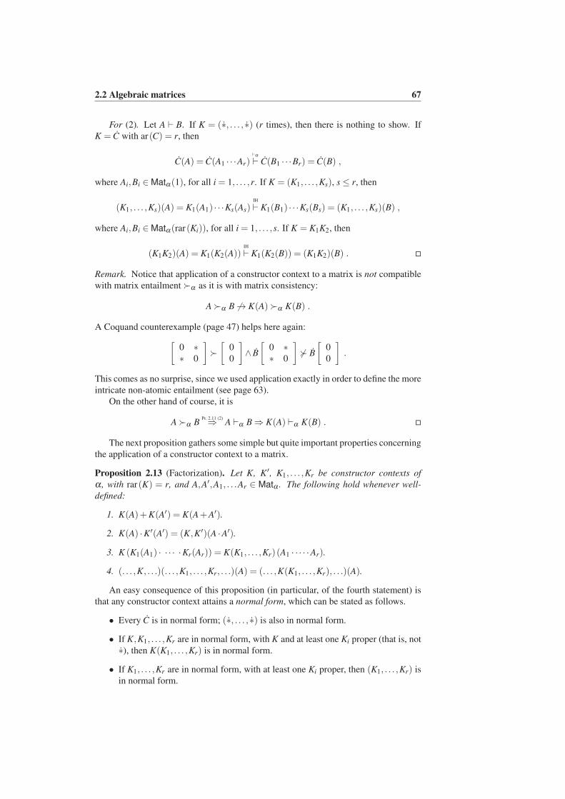
2.2 Algebraic matrices 67
For (2). Let A ⊢ B. If K = (∗, . . . , ∗) (r times), then there is nothing to show. If
K = C with ar(C) = r, then
C(A) = C(A1 · · ·Ar)⊢α
⊢ C(B1 · · ·Br) = C(B) ,
where Ai,Bi ∈Matα(1), for all i = 1, . . . ,r. If K = (K1, . . . ,Ks), s≤ r, then
(K1, . . . ,Ks)(A) = K1(A1) · · ·Ks(As)IH
⊢ K1(B1) · · ·Ks(Bs) = (K1, . . . ,Ks)(B) ,
where Ai,Bi ∈Matα(rar(Ki)), for all i = 1, . . . ,s. If K = K1K2, then
(K1K2)(A) = K1(K2(A))IH
⊢ K1(K2(B)) = (K1K2)(B) .
Remark. Notice that application of a constructor context to a matrix is not compatible
with matrix entailment ≻α as it is with matrix consistency:
A≻α B 6→ K(A)≻α K(B) .
A Coquand counterexample (page 47) helps here again:
[0 ∗∗ 0
]
≻
[0
0
]
∧ B
[0 ∗∗ 0
]
6≻ B
[0
0
]
.
This comes as no surprise, since we used application exactly in order to define the more
intricate non-atomic entailment (see page 63).
On the other hand of course, it is
A≻α BPr. 2.11 (2)⇒ A ⊢α B⇒ K(A) ⊢α K(B) .
The next proposition gathers some simple but quite important properties concerning
the application of a constructor context to a matrix.
Proposition 2.13 (Factorization). Let K, K′, K1, . . . ,Kr be constructor contexts of
α , with rar(K) = r, and A,A′,A1, . . .Ar ∈ Matα . The following hold whenever well-
defined:
1. K(A)+K(A′) = K(A+A′).
2. K(A) ·K′(A′) = (K,K′)(A ·A′).
3. K (K1(A1) · · · · ·Kr(Ar)) = K(K1, . . . ,Kr)(A1 · · · · ·Ar).
4. (. . . ,K, . . .)(. . . ,K1, . . . ,Kr, . . .)(A) = (. . . ,K(K1, . . . ,Kr), . . .)(A).
An easy consequence of this proposition (in particular, of the fourth statement) is
that any constructor context attains a normal form, which can be stated as follows.
• Every C is in normal form; (∗, . . . , ∗) is also in normal form.
• If K,K1, . . . ,Kr are in normal form, with K and at least one Ki proper (that is, not
∗), then K(K1, . . . ,Kr) is in normal form.
• If K1, . . . ,Kr are in normal form, with at least one Ki proper, then (K1, . . . ,Kr) is
in normal form.
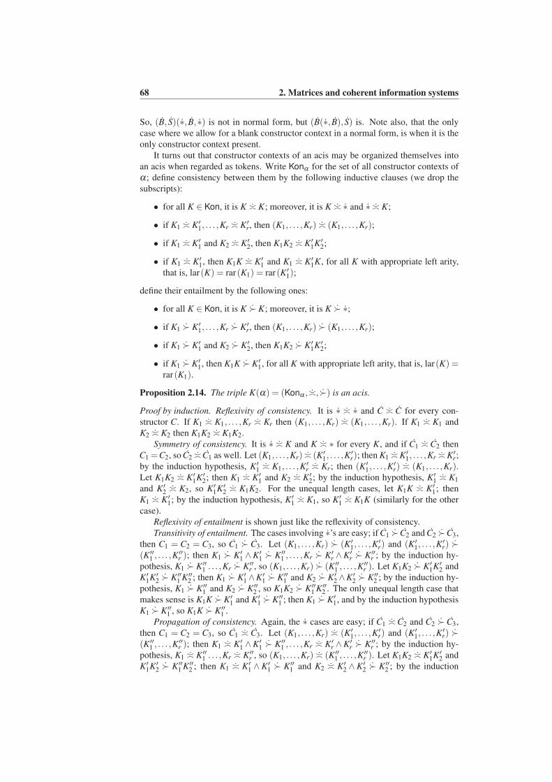
68 2. Matrices and coherent information systems
So, (B, S)(∗, B, ∗) is not in normal form, but (B(∗, B), S) is. Note also, that the only
case where we allow for a blank constructor context in a normal form, is when it is the
only constructor context present.
It turns out that constructor contexts of an acis may be organized themselves into
an acis when regarded as tokens. Write Konα for the set of all constructor contexts of
α; define consistency between them by the following inductive clauses (we drop the
subscripts):
• for all K ∈ Kon, it is K ≍ K; moreover, it is K ≍ ∗ and ∗ ≍ K;
• if K1 ≍ K′1, . . . ,Kr ≍ K′r, then (K1, . . . ,Kr) ≍ (K1, . . . ,Kr);
• if K1 ≍ K′1 and K2 ≍ K′2, then K1K2 ≍ K′1K′2;
• if K1 ≍ K′1, then K1K ≍ K′1 and K1 ≍ K′1K, for all K with appropriate left arity,
that is, lar(K) = rar(K1) = rar(K′1);
define their entailment by the following ones:
• for all K ∈ Kon, it is K ≻ K; moreover, it is K ≻ ∗;
• if K1 ≻ K′1, . . . ,Kr ≻ K′r, then (K1, . . . ,Kr) ≻ (K1, . . . ,Kr);
• if K1 ≻ K′1 and K2 ≻ K′2, then K1K2 ≻ K′1K′2;
• if K1 ≻ K′1, then K1K ≻ K′1, for all K with appropriate left arity, that is, lar(K) =rar(K1).
Proposition 2.14. The triple K(α) = (Konα ,≍,≻) is an acis.
Proof by induction. Reflexivity of consistency. It is ∗ ≍ ∗ and C ≍ C for every con-
structor C. If K1 ≍ K1, . . . ,Kr ≍ Kr then (K1, . . . ,Kr) ≍ (K1, . . . ,Kr). If K1 ≍ K1 and
K2 ≍ K2 then K1K2 ≍ K1K2.
Symmetry of consistency. It is ∗ ≍ K and K ≍ ∗ for every K, and if C1 ≍ C2 then
C1 =C2, so C2 ≍ C1 as well. Let (K1, . . . ,Kr) ≍ (K′1, . . . ,K′r); then K1 ≍K′1, . . . ,Kr ≍K′r;
by the induction hypothesis, K′1 ≍ K1, . . . ,K′r ≍ Kr; then (K′1, . . . ,K
′r) ≍ (K1, . . . ,Kr).
Let K1K2 ≍ K′1K′2; then K1 ≍ K′1 and K2 ≍ K′2; by the induction hypothesis, K′1 ≍ K1
and K′2 ≍ K2, so K′1K′2 ≍ K1K2. For the unequal length cases, let K1K ≍ K′1; then
K1 ≍ K′1; by the induction hypothesis, K′1 ≍ K1, so K′1 ≍ K1K (similarly for the other
case).
Reflexivity of entailment is shown just like the reflexivity of consistency.
Transitivity of entailment. The cases involving ∗’s are easy; if C1 ≻ C2 and C2 ≻ C3,
then C1 = C2 = C3, so C1 ≻ C3. Let (K1, . . . ,Kr) ≻ (K′1, . . . ,K′r) and (K′1, . . . ,K
′r) ≻
(K′′1 , . . . ,K′′r ); then K1 ≻ K′1 ∧K′1 ≻ K′′1 , . . . ,Kr ≻ K′r ∧K′r ≻ K′′r ; by the induction hy-
pothesis, K1 ≻ K′′1 . . . ,Kr ≻ K′′r , so (K1, . . . ,Kr) ≻ (K′′1 , . . . ,K′′r ). Let K1K2 ≻ K′1K′2 and
K′1K′2 ≻ K′′1 K′′2 ; then K1 ≻ K′1∧K′1 ≻ K′′1 and K2 ≻ K′2∧K′2 ≻ K′′2 ; by the induction hy-
pothesis, K1 ≻ K′′1 and K2 ≻ K′′2 , so K1K2 ≻ K′′1 K′′2 . The only unequal length case that
makes sense is K1K ≻ K′1 and K′1 ≻ K′′1 ; then K1 ≻ K′1, and by the induction hypothesis
K1 ≻ K′′1 , so K1K ≻ K′′1 .
Propagation of consistency. Again, the ∗ cases are easy; if C1 ≍ C2 and C2 ≻ C3,
then C1 = C2 = C3, so C1 ≍ C3. Let (K1, . . . ,Kr) ≍ (K′1, . . . ,K′r) and (K′1, . . . ,K
′r) ≻
(K′′1 , . . . ,K′′r ); then K1 ≍ K′1 ∧K′1 ≻ K′′1 , . . . ,Kr ≍ K′r ∧K′r ≻ K′′r ; by the induction hy-
pothesis, K1 ≍ K′′1 . . . ,Kr ≍ K′′r , so (K1, . . . ,Kr) ≍ (K′′1 , . . . ,K′′r ). Let K1K2 ≍ K′1K′2 and
K′1K′2 ≻ K′′1 K′′2 ; then K1 ≍ K′1 ∧K′1 ≻ K′′1 and K2 ≍ K′2 ∧K′2 ≻ K′′2 ; by the induction
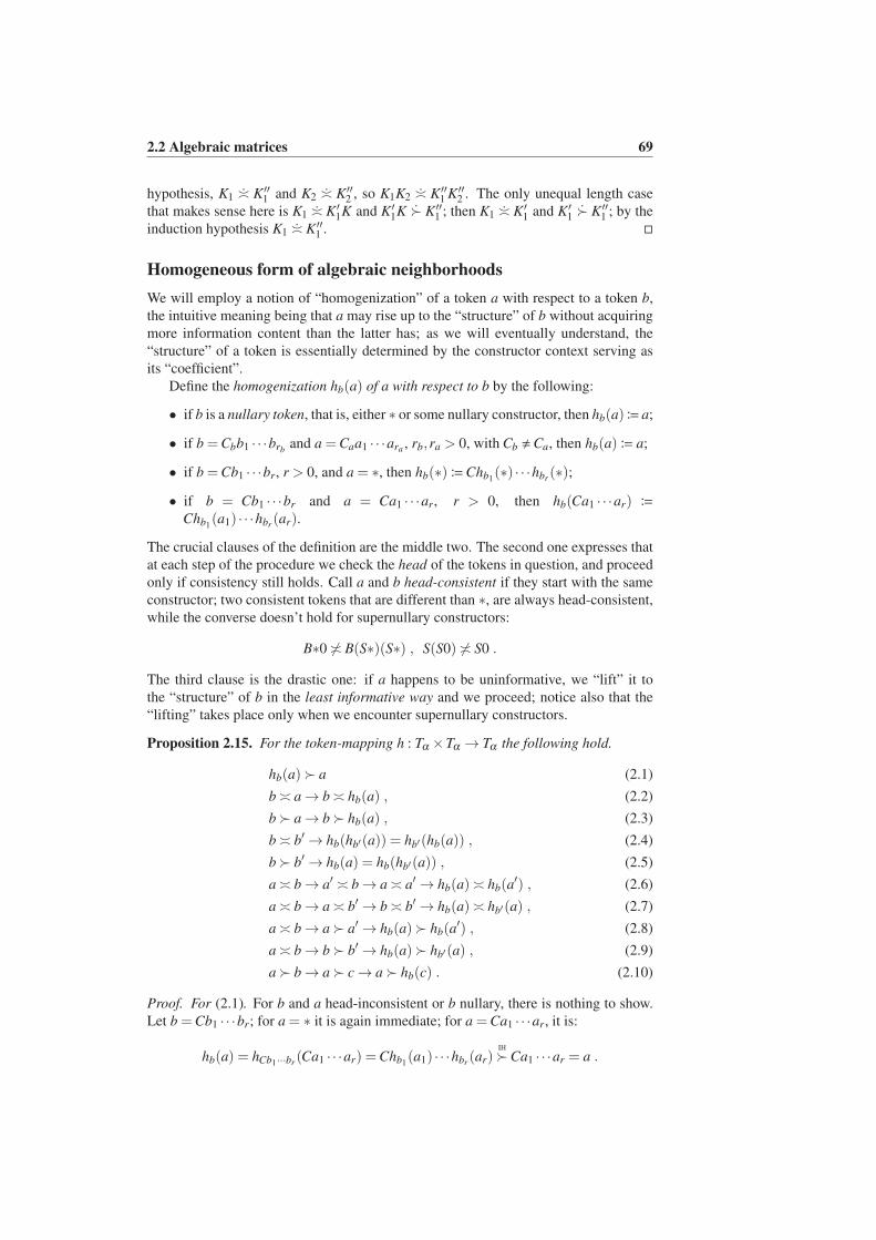
2.2 Algebraic matrices 69
hypothesis, K1 ≍ K′′1 and K2 ≍ K′′2 , so K1K2 ≍ K′′1 K′′2 . The only unequal length case
that makes sense here is K1 ≍ K′1K and K′1K ≻ K′′1 ; then K1 ≍ K′1 and K′1 ≻ K′′1 ; by the
induction hypothesis K1 ≍ K′′1 .
Homogeneous form of algebraic neighborhoods
We will employ a notion of “homogenization” of a token a with respect to a token b,
the intuitive meaning being that a may rise up to the “structure” of b without acquiring
more information content than the latter has; as we will eventually understand, the
“structure” of a token is essentially determined by the constructor context serving as
its “coefficient”.
Define the homogenization hb(a) of a with respect to b by the following:
• if b is a nullary token, that is, either ∗ or some nullary constructor, then hb(a)≔ a;
• if b =Cbb1 · · ·brband a =Caa1 · · ·ara , rb,ra > 0, with Cb ,Ca, then hb(a)≔ a;
• if b =Cb1 · · ·br, r > 0, and a = ∗, then hb(∗)≔Chb1(∗) · · ·hbr
(∗);
• if b = Cb1 · · ·br and a = Ca1 · · ·ar, r > 0, then hb(Ca1 · · ·ar) ≔Chb1
(a1) · · ·hbr(ar).
The crucial clauses of the definition are the middle two. The second one expresses that
at each step of the procedure we check the head of the tokens in question, and proceed
only if consistency still holds. Call a and b head-consistent if they start with the same
constructor; two consistent tokens that are different than ∗, are always head-consistent,
while the converse doesn’t hold for supernullary constructors:
B∗0 6≍ B(S∗)(S∗) , S(S0) 6≍ S0 .
The third clause is the drastic one: if a happens to be uninformative, we “lift” it to
the “structure” of b in the least informative way and we proceed; notice also that the
“lifting” takes place only when we encounter supernullary constructors.
Proposition 2.15. For the token-mapping h : Tα ×Tα → Tα the following hold.
hb(a)≻ a (2.1)
b≍ a→ b≍ hb(a) , (2.2)
b≻ a→ b≻ hb(a) , (2.3)
b≍ b′→ hb(hb′(a)) = hb′(hb(a)) , (2.4)
b≻ b′→ hb(a) = hb(hb′(a)) , (2.5)
a≍ b→ a′ ≍ b→ a≍ a′→ hb(a)≍ hb(a′) , (2.6)
a≍ b→ a≍ b′→ b≍ b′→ hb(a)≍ hb′(a) , (2.7)
a≍ b→ a≻ a′→ hb(a)≻ hb(a′) , (2.8)
a≍ b→ b≻ b′→ hb(a)≻ hb′(a) , (2.9)
a≻ b→ a≻ c→ a≻ hb(c) . (2.10)
Proof. For (2.1). For b and a head-inconsistent or b nullary, there is nothing to show.
Let b =Cb1 · · ·br; for a = ∗ it is again immediate; for a =Ca1 · · ·ar, it is:
hb(a) = hCb1···br(Ca1 · · ·ar) =Chb1
(a1) · · ·hbr(ar)
IH
≻Ca1 · · ·ar = a .
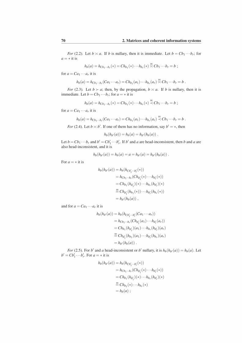
70 2. Matrices and coherent information systems
For (2.2). Let b ≍ a. If b is nullary, then it is immediate. Let b = Cb1 · · ·br; for
a = ∗ it is
hb(a) = hCb1···br(∗) =Chb1
(∗) · · ·hbr(∗)
IH
≍Cb1 · · ·br = b ;
for a =Ca1 · · ·ar it is
hb(a) = hCb1···br(Ca1 · · ·ar) =Chb1
(a1) · · ·hbr(ar)
IH
≍Cb1 · · ·br = b .
For (2.3). Let b ≻ a; then, by the propagation, b ≍ a. If b is nullary, then it is
immediate. Let b =Cb1 · · ·br; for a = ∗ it is
hb(a) = hCb1···br(∗) =Chb1
(∗) · · ·hbr(∗)
IH
≺Cb1 · · ·br = b ;
for a =Ca1 · · ·ar it is
hb(a) = hCb1···br(Ca1 · · ·ar) =Chb1
(a1) · · ·hbr(ar)
IH
≺Cb1 · · ·br = b .
For (2.4). Let b≍ b′. If one of them has no information, say b′ = ∗, then
hb(hb′(a)) = hb(a) = hb′(hb(a)) .
Let b =Cb1 · · ·br and b′ =Cb′1 · · ·b′r. If b′ and a are head-inconsistent, then b and a are
also head-inconsistent, and it is
hb(hb′(a)) = hb(a) = a = hb′(a) = hb′(hb(a)) .
For a = ∗ it is
hb(hb′(a)) = hb(hCb′1···b′r(∗))
= hCb1···br(Chb′1
(∗) · · ·hb′r(∗))
=Chb1(hb′1
)(∗) · · ·hbr(hb′r
)(∗)
IH=Chb′1
(hb1(∗)) · · ·hb′r
(hbr(∗))
= hb′(hb(a)) ,
and for a =Ca1 · · ·ar it is
hb(hb′(a)) = hb(hCb′1···b′r(Ca1 · · ·ar))
= hCb1···br(Chb′1
(a1) · · ·hb′r(ar))
=Chb1(hb′1
)(a1) · · ·hbr(hb′r
)(ar)
IH=Chb′1
(hb1)(a1) · · ·hb′r
(hbr)(ar)
= hb′(hb(a)) .
For (2.5). For b′ and a head-inconsistent or b′ nullary, it is hb(hb′(a)) = hb(a). Let
b′ =Cb′1 · · ·b′r. For a = ∗ it is
hb(hb′(a)) = hb(hCb′1···b′r(∗))
= hCb1···br(Chb′1
(∗) · · ·hb′r(∗))
=Chb1(hb′1
)(∗) · · ·hbr(hb′r
)(∗)
IH=Chb1
(∗) · · ·hbr(∗)
= hb(a) ;
2.2 Algebraic matrices 71
for a =Ca1 · · ·ar it is
hb(hb′(a)) = hb(hCb′1···b′r(Ca1 · · ·ar))
= hCb1···br(Chb′1
(a1) · · ·hb′r(ar))
=Chb1(hb′1
)(a1) · · ·hbr(hb′r
)(ar)
IH=Chb1
(a1) · · ·hbr(ar)
= hb(a) .
For (2.6). If b is nullary then it is immediately hb(a) = a ≍ a′ = hb(a′). Let b =
Cb1 · · ·br; for a = a′ = ∗, there is nothing to show; let a =Ca1 · · ·ar; if a′ = ∗, then
hb(a) = hCb1···br(Ca1 · · ·ar)
=Chb1(a1) · · ·hbr
(ar)IH
≍Chb1(∗) · · ·hbr
(∗)
= hCb1···br(∗)
= hb(a′) ;
if a′ =Ca′1 · · ·a′r, then
hb(a) = hCb1···br(Ca1 · · ·ar)
=Chb1(a1) · · ·hbr
(ar)IH
≍Chb1(a′1) · · ·hbr
(a′r)
= hCb1···br(Ca′1 · · ·a
′r)
= hb(a′) .
For (2.7). If b and b′ are nullary, then hb(a) = a = hb′(a). Let b′ =Cb′1 · · ·b′r. If b
is nullary, then for a = ∗ it is immediately hb(a) = ∗ ≍ hb′(a), and for a =Ca1 · · ·ar, it
is
hb(a) = a =Ca1 · · ·ar(2.1)
≍ Chb′1(a1) · · ·hb′r
(ar) = hCb′1···b′r(Ca1 · · ·ar) = hb′(a) .
Further, let b =Cb1 · · ·br; if a = ∗, then
hb(a) = hCb1···br(∗)
=Chb1(∗) · · ·hbr
(∗)IH
≍Chb′1(∗) · · ·hb′r
(∗)
= hCb′1···b′r(∗)
= hb′(a) ,
whereas, if a =Ca1 · · ·ar, it is
hb(a) = hCb1···br(a1 · · ·ar)
=Chb1(a1) · · ·hbr
(ar)IH
≍Chb′1(a1) · · ·hb′r
(ar)
= hCb′1···b′r(Ca1 · · ·ar)
= hb′(a) .
72 2. Matrices and coherent information systems
For (2.8). Let a ≻ a′ and b ≍ a; by the propagation, it is also b ≍ a′. Let b =Cb1 · · ·Cbr. If a = ∗, then necessarily a′ = ∗, and hb(a) = hb(a
′). Let further a =Ca1 · · ·ar; for a′ = ∗, it is
hb(a) = hCb1···br(Ca1 · · ·ar)
=Chb1(a1) · · ·hbr
(ar)IH
≻Chb1(∗) · · ·hbr
(∗)
= hCb1···br(∗)
= hb(a′) ,
whereas, if a′ =Ca′1 · · ·a′r, it is
hb(a) = hCb1···br(Ca1 · · ·ar)
=Chb1(a1) · · ·hbr
(ar)IH
≻Chb1(a′1) · · ·hbr
(a′r)
= hCb1···br(Ca′1 · · ·a
′r)
= hb(a′) .
For (2.9). Let b≻ b′ and b≍ a; by the propagation, it is also b′ ≍ a. If b is nullary,
then b′ must also be nullary, and hb(a) = a = hb′(a). Let b =Cb1 · · ·br. For b′ nullary,
it is hb(a)(2.1)
≻ a = hb′(a). Let then b′ =Cb′1 · · ·b′r as well. If a = ∗ then
hb(a) = hCb1···br(∗)
=Chb1(∗) · · ·hbr
(∗)IH
≻Chb′1(∗) · · ·hb′r
(∗)
= hCb′1···b′r(∗)
= hb′(a) ;
if a =Ca1 · · ·ar, it is
hb(a) = hCb1···br(Ca1 · · ·ar)
=Chb1(a1) · · ·hbr
(ar)IH
≻Chb′1(a1) · · ·hb′r
(ar)
= hCb′1···b′r(Ca1 · · ·ar)
= hb′(a) .
For (2.10). Let a≻ b and a≻ c; then it is b≍ c. If a is nullary then b, c must also
be nullary, so we don’t have anything to do. Let a = Ca1 · · ·ar. For b nullary, there is
again nothing to show, so let also b =Cb1 · · ·br. Now if c is nullary we have
hb(c) = hCb1···br(∗) =Chb1
(∗) · · ·hbr(∗)
IH
≺Ca1 · · ·ar = a ,
where if c =Cc1 · · ·cr, we have
hb(c) = hCb1···br(Cc1 · · ·cr) =Chb1
(c1) · · ·hbr(cr)
IH
≺Ca1 · · ·ar = a .
2.2 Algebraic matrices 73
Now we gradually extend the notion of homogenization to matrices, in the follow-
ing way:
hb1+···+bl′(a)≔ hbl′
· · ·hb1(a) ,
hV (a1 + · · ·+al)≔ hV (a1)+ · · ·+hV (al) ,
hV1···Vr(U1 · · ·Ur)≔ hV1(U1) · · ·hVr(Ur) ,
where Ui’s and Vi’s, i = 1, . . . ,r, are lists of equal length, and we write h1 · · ·hl for
h1 · · · hl to save space. Put more bluntly, the homogenization hB(A) of A ∈ Arrα(r, l)with respect to B ∈ Arrα(r, l
′) is defined by
h∏
ri=1 ∑
l′
j′=1bi j′
(r
∏i=1
l
∑j=1
ai j
)
≔
r
∏i=1
l
∑j=1
hbil′· · ·hbi1
(ai j) ;
it is obviously well-defined.4 We will just write h(A) for hA(A); call A homogeneous if
it is already A = h(A).
Proposition 2.16. The mapping h : Arrα(r, l′)×Arrα(r, l)→ Arrα(r, l) is well-defined
and satisfies the following.
hB(A)≻ A , (2.11)
B≍ B′→ hB(hB′(A)) = hB′(hB(A)) , (2.12)
B≻ B′→ hB(A) = hB(hB′(A)) , (2.13)
A≍ B→ (A′ ≍ B∨A≍ B′)→ A′ ≍ B′
→ A≍ A′→ B≍ B′→ hB(A)≍ hB′(A′) , (2.14)
A≍ B→ A≻ A′→ B≻ B′→ hB(A)≻ hB′(A′) , (2.15)
A≍ B→ A ⊢ A′→ hB(A) ⊢ hB(A′) , (2.16)
A≍ B→ B ⊢ B′→ hB(A) ⊢ hB′(A) , (2.17)
A ⊢ h(A) , (2.18)
h(K(A)) = K(h(A)) , (2.19)
A = K(B)→ (A = h(A)↔ B = h(B)) , (2.20)
(2.21)
Proof. That the mapping is well-defined is clear. For the following, let A ∈Mat(r, lA),B ∈Mat(r, lB), A′ ∈Mat(r, lA′), and B′ ∈Mat(r, lB′).
For (2.11). It is
hB(A) =r
∏i=1
lA
∑jA=1
hbilB· · ·hbi1
(ai jA)(2.1)
≻r
∏i=1
lA
∑jA=1
ai jA = A .
4Notice though that the value in general depends on the order of the elements in the list; for example,
hS∗+B∗∗(∗) = S∗ , B∗∗= hB∗∗+S∗(∗) .
This is not the case though when the list is consistent, that is, a neighborhood, as we will readily see.
74 2. Matrices and coherent information systems
For (2.12). It is
hB(hB′(A)) =r
∏i=1
lA
∑jA=1
hbilB· · ·hbi1
hb′il
B′· · ·hb′i1
(ai jA)
(2.4)=
r
∏i=1
lA
∑jA=1
hb′il
B′· · ·hb′i1
hbilB· · ·hbi1
(ai jA)
= hB′(hB(A)) .
For (2.13). It is
hB(hB′(A)) =r
∏i=1
lA
∑jA=1
hbilB· · ·hbi1
hb′il
B′· · ·hb′i1
(ai jA)
(2.4), (2.5)=
r
∏i=1
lA
∑jA=1
hbilB· · ·hbi1
(ai jA)
= hB(A) .
For (2.14). Let A≍ B, A′ ≍ B, and then A≍ A′, and B≍ B′. It is
hB(A) =r
∏i=1
lA
∑jA=1
hbilB· · ·hbi1
(ai jA)
(2.6)
≍r
∏i=1
lA′
∑jA′=1
hbilB· · ·hbi1
(a′i jA′)
(2.7), (2.4), (2.5)
≍r
∏i=1
lA′
∑jA′=1
hb′il
B′· · ·hb′i1
(a′i jA′)
= hB′(A′) .
The assumption that A′ ≍ B enabled us to take the second step; we would need the
alternative assumption A≍ B′ if we wanted to use (2.7) first, and then (2.6).
For (2.15). Let A≍ B, A≻ A′, and B≻ B′. It is
hB(A) =r
∏i=1
lA
∑jA=1
hbilB· · ·hbi1
(ai jA)
(2.8)
≻r
∏i=1
lA′
∑jA′=1
hbilB· · ·hbi1
(a′i jA′)
(2.9), (2.4), (2.5)
≻r
∏i=1
lA′
∑jA′=1
hb′il
B′· · ·hb′i1
(a′i jA′)
= hB′(A′) .
For the following statements, since entailment between matrices works row-wise,
we restrict our arguments to lists with no loss of generality. Furthermore, because of
(2.5), we may safely assume that the lists V , V ′, with respect to which we homogenize,
will consist of tokens where none entails some other (we make this assumption in the
2.2 Algebraic matrices 75
proofs of (2.16) and (2.17)). In this case, for a non-blank list V of length l′ and a list U
of length l, such that U ≍V , we either have U non-blank as well, in which case
hV (U) = hb1+···+bl′(a1 + · · ·+al)
= hb1+···+bl′(a1)+ · · ·+hb1+···+bl′
(al)
= hb1· · ·hbl′
(a1)+ · · ·+hb1· · ·hbl′
(al)
= hCb11···br1· · ·hCb1l′ ···brl′
(Ca11 · · ·ar1)
+ · · ·+hCb11···br1· · ·hCb1l′ ···brl′
(Ca1l · · ·arl)
=C(hb11· · ·hb1l′
(a11)) · · ·(hbr1· · ·hbrl′
(ar1))
+ · · ·+C(hb11· · ·hb1l′
(a1l)) · · ·(hbr1· · ·hbrl′
(arl))
= C
hb11· · ·hb1l′
(a11) · · · hb11· · ·hb1l′
(a1l)...
. . ....
hbr1· · ·hbrl′
(ar1) · · · hbr1· · ·hbrl′
(arl)
,
that is,
hC(V1···Vr)(C(U1 · · ·Ur)) = C(hV1
(U1) · · ·hVr(Ur)) , (2.22)
or U is a blank list, U = ∗1,l , in which case we similarly obtain
hC(V1···Vr)(∗1,l) = C(hV1
(∗1,l) · · ·hVr(∗1,l)) . (2.23)
For (2.16). We show that
U ≍V →U ⊢U ′→ hV (U) ⊢ hV (U′) ,
for U,U ′,V lists. Let U ≍ V and U ⊢U ′. We proceed by induction on V (under our
assumption above). If V is a nullary (more precisely, it consists of a single nullary
token), then hV (U) = U ⊢U ′ = hV (U′), so let V = b1 + · · ·+ blV = C(V1 · · ·Vr). For
U = ∗1,lU , it must also be that U ′ = ∗1,lU ′ , so
hV (U) = hV (∗)+ · · ·+hV (∗)︸ ︷︷ ︸
lU times
≻ hV (∗)+ · · ·+hV (∗)︸ ︷︷ ︸
lU ′ times
= hV (U′) .
For U = C(U1 · · ·Ur), if U ′ = ∗1,lU ′ , it is
hV (U) = hC(V1···Vr)(C(U1 · · ·Ur))
(2.22)= C(hV1
(U1) · · ·hVr(Ur))IH
⊢ C(hV1(∗1,lU ′ ) · · ·hVr(∗
1,lU ′ ))(2.23)= hC(V1···Vr)
(∗1,lU ′ )
= hV (U′) ,
whereas if U ′ = C(U ′1 · · ·U
′r) it is
hV (U) = hC(V1···Vr)(C(U1 · · ·Ur))
(2.22)= C(hV1
(U1) · · ·hVr(Ur))IH
⊢ C(hV1(U ′
1) · · ·hVr(U′r))
(2.22)= hC(V1···Vr)
(U ′)
= hV (U′) .
76 2. Matrices and coherent information systems
Finally, if U∗ ⊇∗ U , then
hV (U∗) = hV (~∗+a1 +~∗+ · · ·+~∗+alU +~∗)
= hV (~∗)+hV (a1)+hV (~∗)+ · · ·+hV (~∗)+hV (alU )+hV (~∗)
≻ hV (a1)+ · · ·+hV (alU )
= hV (a1 + · · ·+alU )
= hV (U)IH
⊢ hV (U′) .
For (2.17). We show that
U ≍V →V ⊢V ′→ hV (U) ⊢ hV ′(U) ,
for U,V,V ′ appropriate lists. Let U ≍ V and V ⊢ V ′. According to our assumption,
let first V be nullary, V ′ must also be nullary; then hV (U) = U = hV ′(U). Then let
V = C(V1 · · ·Vr); if V ′ is still a nullary, then, by (2.11), hV (U) ≻U = hV ′(U); if V ′ =C(V ′1 · · ·V
′r ), then for U = ∗1,lU it is
hV (U) = hC(V1···Vr)(∗1,lU )
(2.23)= C(hV1
(∗1,lU ) · · ·hVr(∗1,lU ))
IH
⊢ C(hV ′1(∗1,lU ) · · ·hV ′r
(∗1,lU ))
(2.23)= hC(V ′1···V
′r )(∗1,lU )
= hV ′(U) ,
for U = C(U1 · · ·Ur) it is
hV (U) = hC(V1···Vr)(C(U1 · · ·Ur))
(2.22)= C(hV1
(U1) · · ·hVr(Ur))IH
⊢ C(hV ′1(U1) · · ·hV ′r
(Ur))
(2.22)= hC(V ′1···V
′r )(C(U1 · · ·Ur))
= hV ′(U) ,
and for U∗ ⊇∗ U it is
hV (U∗)
(2.16)
⊢ hV (U)IH
⊢ hV ′(U)(2.16)
⊢ hV ′(U∗) .
For (2.18). We show that
U ⊢ h(U) ,
for any list U . If U is a nullary, then immediately h(U) =U . If U = C(U1 · · ·Ur); then
h(U) = h(C(U1 · · ·Ur))(2.22)= C(h(U1) · · ·h(Ur))
IH
⊣ C(U1 · · ·Ur) =U .
Finally, if U∗ ⊇∗ U , then
U∗ ≻UIH
⊢ h(U) = hU (U)(2.17)
⊢ hU∗(U)(2.16)
⊢ hU∗(U∗) = h(U∗) .
2.2 Algebraic matrices 77
For (2.19). By induction on the constructor context K. For K = ∗, it is immediately
h(∗(A)) = h(A) = ∗(A). For K = C, it is
h(C(A)) = h(C(U1 · · ·Ur))(2.22)= C(h(U1) · · ·h(Ur)) = C(h(A)) .
For K = (K1, . . . ,Km), it is
h(K(A)) = h((K1, . . . ,Km)(A1 · · ·Am))
= h(K1(A1) · · ·Km(Am))
= h(K1(A1)) · · ·h(Km(Am))IH= K1(h(A1)) · · ·Km(h(Am))
= (K1, . . . ,Km)(h(A1) · · ·h(Am))
= K(h(A)) .
Finally, for K = K1K2, it is
h(K(A)) = h(K1K2(A))
= h(K1(K2(A1)))IH= K1(h(K2(A1)))IH= K1(K2(h(A1)))
= K1K2(h(A))
= K(h(A)) .
For (2.20). Let A = K(B). We have
A = h(A)⇔ K(B) = h(K(B))(2.19)⇔ K(B) = K(h(B))⇔ B = h(B) .
Now we have the necessary means to state and prove the matrix form theorem.
Theorem 2.17 (Finitary matrix form). Let α be a finitary algebra. For every homoge-
neous matrix A ∈Matα(r, l), there exist a unique constructor context KA ∈ Konα(r,r′)
in normal form, r′ ≥ r, and a unique basic matrix MA ∈Matα(r′, l), such that
A = KA(MA) .
Call KA(MA) the matrix form of A, KA the basic coefficient of A, and MA the basis
of A.
Proof by induction on the complexity of A. Let A ∈ Matα(r, l). If A is already basic,
then simply KA = (∗, . . . , ∗) (r times) and MA = A.
If A = K(A′), for some K ∈ Konα(r,r′) and A′ ∈ Matα(r
′, l), then, by (2.20), A′ is
also homogeneous, so by the induction hypothesis it has a matrix form KA′(MA′), with
KA′ ∈ Konα(r′,r′′) and MA′ ∈Matα(r
′′, l) (it is r ≤ r′ ≤ r′′); then
A = K(A′) = K(KA′(MA′)) = (KKA′)(MA′) ;
now if KA′ = (∗, . . . , ∗) then r′ = r′′ and KA = K ∈ Konα(r,r′′), otherwise KA = KKA′ ∈
Konα(r,r′′); for the basis, it is MA = MA′ ∈Matα(r
′′, l).
78 2. Matrices and coherent information systems
The matrix form, the basic coefficient, and the basis of an arbitrary matrix A are
defined to be the matrix form, the basic coefficient, and the basis of its homogenization
h(A) respectively, in symbols
KA ≔ Kh(A)∧MA ≔Mh(A) ;
so the theorem in effect says that every matrix has a matrix form, which is unique up
to homogenization.
Example. Let α be given by a nullary constructor 0, a unary S, a binary B, and a ternary
C; we write ∗ for ∗α . Consider the list
U =C(B0∗)∗∗+C(B∗0)(B∗0)∗+C∗∗(SS0)+∗ .
Its homogenization h(U) is given by
C(B0∗)(B∗∗)(SS∗)+C(B∗0)(B∗0)(SS∗)+C(B∗∗)(B∗∗)(SS0)+C(B∗∗)(B∗∗)(SS∗) .
Exhaustive factorization proceeds as follows:
C(B0∗)(B∗∗)(SS∗)+C(B∗0)(B∗0)(SS∗)+C(B∗∗)(B∗∗)(SS0)+C(B∗∗)(B∗∗)(SS∗)
= C(
(B0∗)(B∗∗)(SS∗)+(B∗0)(B∗0)(SS∗)+(B∗∗)(B∗∗)(SS0)+(B∗∗)(B∗∗)(SS∗))
= C(B, ∗, ∗)(
0∗(B∗∗)(SS∗)+∗0(B∗0)(SS∗)+∗∗(B∗∗)(SS0)+∗∗(B∗∗)(SS∗))
= C(B, ∗, ∗)(∗, ∗, B, ∗)(
0∗∗∗(SS∗)+∗0∗0(SS∗)+∗∗∗∗(SS0)+∗∗∗∗(SS∗))
= C(B, ∗, ∗)(∗, ∗, B, ∗)(∗, ∗, ∗, ∗, S)(
0∗∗∗(S∗)+∗0∗0(S∗)+∗∗∗∗(S0)+∗∗∗∗(S∗))
= C(B, ∗, ∗)(∗, ∗, B, ∗)(∗, ∗, ∗, ∗, S)(∗, ∗, ∗, ∗, S)(
0∗∗∗∗+∗0∗0∗+∗∗∗∗0+∗∗∗∗∗)
= C(B, B, SS)(
0∗∗∗∗+∗0∗0∗+∗∗∗∗0+∗∗∗∗∗)
so the matrix form of U is
U = C(B, B, SS)
0 ∗ ∗ ∗∗ 0 ∗ ∗∗ ∗ ∗ ∗∗ 0 ∗ ∗∗ ∗ 0 ∗
.
Using normal forms
Here we take a break and demonstrate how useful the matrix form can be in practice.
Namely, we show that it readily provides a very clear and insightful characterization of
entailment, which in turn leads rather automatically to a simple atomic characterization.
We will use two natural notions of equivalence for matrices. Call A,B ∈ Matαatomically equivalent (or atomically equientailing), and write A ∼A B, when A ≻ B∧B ≻ A; call them just equivalent (or equientailing), and write A ∼ B, if A ⊢ B∧B ⊢ A.
For a consistent list U ∈ Lstα(l), define its induced set set(U) by
a ∈ set(U)≔l
∃j=1
U( j) = a .
Proposition 2.18. The following hold whenever well-defined.
2.2 Algebraic matrices 79
1. If A∼A B then A∼ B.
2. It is A∼A B if and only if set(Ai) = set(Bi), for all i = 1, . . . ,r.
3. It is
A∼A B↔ ∀M(A≻M ↔ B≻M) ,
A∼ B↔ ∀M(A ⊢M ↔ B ⊢M) .
4. It is
A∼ A′→ A≍ B→ A′ ≍ B ,
A∼A A′→ B∼A B′→(
A+B∼A A′+B′∧A ·B∼A A′ ·B′)
,
A∼ A′→ B∼ B′→(
A+B∼ A′+B′∧A ·B∼ A′ ·B′)
.
Proof. The first two statements are easy to see. As for 3, it is an immediate conse-
quence of transitivity of entailment, atomic as well as not.
For 4. The first clause is an easy consequence of propagation of consistency
through entailment. For the second clause, let A ∼A A′ and B ∼A B′; then for any
matrix M it is
A+B≻M ⇔r
∀i=1
lM
∀jM=1
(lA
∃jA=1
ai jA ≻ ci jM ∨lB
∃jB=1
bi jB ≻ ci jM
)
⇔r
∀i=1
lM
∀jM=1
(lA′
∃jA′=1
a′i jA′≻ ci jM ∨
lB′
∃jB′=1
b′i jB′≻ ci jM
)
⇔ A′+B′ ≻M ,
so A+B∼A A′+B′; similarly we have
A ·B≻M ⇔r
∀i=1
lM
∀jM=1
l
∃j=1
ai j ≻ ci jM ⇔r
∀i=1
lM
∀jM=1
l′
∃j′=1
a′i j′ ≻ ci jM ⇔ A′ ·B′ ≻M ,
that is, A ·B ∼A A′ ·B′. For the third clause, more swiftly, from A ∼ A′ and B ∼ B′ we
obtain
A ⊢ A′∧B ⊢ B′trns⇒ A+B ⊢ A′∧A+B ⊢ B′⇒ A+B ⊢ A′+B′ ,
and similarly A′+B′ ⊢ A+B; moreover, if A ∼ A′ ∧B ∼ B′, then AB ∼ A′B′ by the
definition of entailment for matrices.
Characterization of consistency and entailment through homogenization
Some inspection of examples leads us to acknowledge three different cases when
checking if U ⊢ a, with respective normal forms KU (MU ) and Ka(Ma). For simplicity
(which does not harm generality, as we will show) we assume that both basic matrices
have the same row dimension.
• It is U ≍ a and U ⊢ a; in this case it is necessarily both KU ≻ Ka and MU ≻Ma.
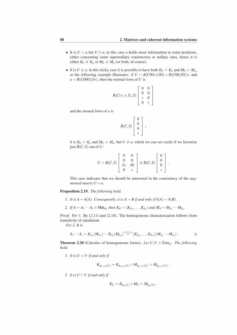
80 2. Matrices and coherent information systems
• It is U ≍ a but U 6⊢ a; in this case a holds more information in some positions,
either concerning some supernullary constructors or nullary ones, hence it is
either KU 6≻ Ka or MU 6≻Ma (or both, of course).
• It is U 6≍ a; in this tricky case it is possible to have both KU ≻ Ka and MU ≻Ma,
as the following example illustrates: if U = B(C00∗)(S0) +B(C00(S0))∗ and
a = B(C000)(S∗), then the normal form of U is
B(C(∗, ∗, S), S)
0 0
0 0
∗ 0
0 ∗
and the normal form of a is
B(C, S)
0
0
0
∗
;
it is KU ≻ Ka and MU ≻Ma, but U 6≍ a, which we can see easily if we factorize
just B(C, S) out of U :
U = B(C, S)
0 0
0 0
S∗ S0
0 ∗
6≍ B(C, S)
0
0
0
∗
.
This case indicates that we should be interested in the consistency of the aug-
mented matrix U +a.
Proposition 2.19. The following hold.
1. It is A∼ h(A). Consequently, it is A∼ B if and only if h(A)∼ h(B).
2. If A = A1 · · ·As ∈Matα , then KA = (KA1, . . . ,KAs) and MA = MA1
· · ·MAs .
Proof. For 1. By (2.11) and (2.18). The homogeneous characterization follows from
transitivity of entailment.
For 2. It is
A1 · · ·As = KA1(MA1
) · · ·KAs(MAs)P.2.13 (3)= (KA1
, . . . ,KAs)(MA1· · ·MAs) .
Theorem 2.20 (Calculus of homogeneous forms). Let U,V ∈ Conα . The following
hold.
1. It is U ≍V if and only if
KhU+V (U) = KhU+V (V )∧MhU+V (U) ≍MhU+V (V ) .
2. It is U ⊢V if and only if
KU = KhU (V )∧MU ≻MhU (V ) .
2.2 Algebraic matrices 81
Proof. By Proposition 2.19. 1, it is U ≍ V and U ⊢ V if and only if h(U) ≍ h(V ) and
h(U) ⊢ h(V ) respectively. Based on this observation, we may assume that the lists we
consider are homogeneous, with no loss of generality.
For 1. If both lists are nullary, then, for W ≔U +V = ∗1,l+l′ ,
KhW (U) = KU = ∗= KV = KhW (V )
and
U ≍V ⇔MhW (U) = MU =U ≍V = MV = MhW (V ) .
If U = C(U1 · · ·Ur) and V = ∗1,l′ , for W ≔U +V we have
hW (U)(2.13)= h(U)
hW (V )(2.13)= hU (V ) = hC(U1···Ur)
(∗1,l′)(2.23)= C
(
hU1(∗1,l′) · · ·hUr(∗
1,l′))
;
by the induction hypothesis, for Wi ≔Ui +∗1,l′ , i = 1, . . . ,r, it is
r
∀i=1
Ui ≍ ∗1,l′ ⇔
r
∀i=1
(
KhWi(Ui) = K
hWi(∗1,l′ )
∧MhWi(Ui) ≍M
hWi(∗1,l′ )
)
⇔(
KhW1(U1), . . . ,KhWr (Ur)
)
=(
KhW1
(∗1,l′ ), . . . ,K
hWr (∗1,l′ )
)
∧MhW1(U1) · · ·MhWr (Ur) ≍M
hW1(∗1,l′ )
· · ·MhWr (∗
1,l′ )
⇔C(
KhW1(U1), . . . ,KhWr (Ur)
)
= C(
KhW1
(∗1,l′ ), . . . ,K
hWr (∗1,l′ )
)
∧MhW1(U1) · · ·MhWr (Ur) ≍M
hW1(∗1,l′ )
· · ·MhWr (∗
1,l′ )
P.2.19⇔KhW (U) = KhW (V )∧MhW (U) ≍MhW (V ) .
If U = C(U1 · · ·Ur) and V = C(V1 · · ·Vr), for W ≔U +V and Wi ≔Ui +Vi, i = 1, . . . ,r,
we have
U ≍V ⇔r
∀i=1
Ui ≍Vi
IH⇔
r
∀i=1
(
KhWi(Ui) = KhWi
(Vi)∧MhWi(Ui) ≍MhWi
(Vi)
)
⇔(
KhW1(U1), . . . ,KhWr (Ur)
)
=(
KhW1(V1), . . . ,KhWr (Vr)
)
∧MhW1(U1) · · ·MhWr (Ur) ≍MhW1
(V1) · · ·MhWr (Vr)
⇔C(
KhW1(U1), . . . ,KhWr (Ur)
)
= C(
KhW1(V1), . . . ,KhWr (Vr)
)
∧MhW1(U1) · · ·MhWr (Ur) ≍MhW1
(V1) · · ·MhWr (Vr)
P.2.19⇔KhW (U) = KhW (V )∧MhW (U) ≍MhW (V ) .
For 2. If both lists are nullary, then
KU = ∗= KV = KhU (V )
and
U ⊢V ⇔MU =U ≻V = MV = MhU (V ) .
82 2. Matrices and coherent information systems
If U = C(U1 · · ·Ur) and V = ∗1,l′ , we have
hU (V ) = hC(U1···Ur)(∗1,l′)
(2.23)= C
(
hU1(∗1,l′) · · ·hUr(∗
1,l′))
;
by the induction hypothesis, it is
r
∀i=1
Ui ⊢ ∗1,l′ ⇔
r
∀i=1
(
KUi= K
hUi(∗1,l′ )
∧MUi≻M
hUi(∗1,l′ )
)
⇔(KU1, . . . ,KUr) =
(
KhU1
(∗1,l′ ), . . . ,K
hUr (∗1,l′ )
)
∧MU1· · ·MUr ≻M
hU1(∗1,l′ )
· · ·MhUr (∗
1,l′ )
⇔C (KU1, . . . ,KUr) = C
(
KhU1
(∗1,l′ ), . . . ,K
hUr (∗1,l′ )
)
∧MU1· · ·MUr ≻M
hU1(∗1,l′ )
· · ·MhUr (∗
1,l′ )
P.2.19⇔KU = KhU (V )∧MU ≻MhU (V ) .
If U = C(U1 · · ·Ur) and V = C(V1 · · ·Vr), we have
U ⊢V ⇔r
∀i=1
Ui ⊢Vi
IH⇔
r
∀i=1
(
KUi= KhUi
(Vi)∧MUi≻MhUi
(Vi)
)
⇔(KU1, . . . ,KUr) =
(
KhU1(V1), . . . ,KhUr (Vr)
)
∧MU1· · ·MUr ≻MhU1
(V1) · · ·MhUr (Vr)
⇔C (KU1, . . . ,KUr) = C
(
KhU1(V1), . . . ,KhUr (Vr)
)
∧MU1· · ·MUr ≻MhU1
(V1) · · ·MhUr (Vr)
P.2.19⇔KU = KhU (V )∧MU ≻MhU (V ) .
Characterization of consistency and entailment through eigentokens
Let U ∈ Lstα(l); a token e ∈ Tα is an eigentoken (or a characteristic token) of U , if it
is equivalent to U , that is, if
U ∼ e⇔ ∀b∈Tα
(U ⊢ b↔ e ⊢ b) .
An eigenvector (or a characteristic vector) of a matrix A = U1 · · ·Ur ∈ Matα(r, l) is a
vector E = e1 · · ·er ∈ Vecα(r,1) where ei is an eigenvector of Ui, for i = 1, . . . ,r.
Proposition 2.21. Let α be a finitary algebra.
1. For every A ∈Matα(r) there exists a unique eigenvector e(A) ∈ Vecα(r).
2. If A = K(B) then e(A) = K (e(B)).
3. The eigenvector of any A ∈Matα is given by KA(e(MA)).
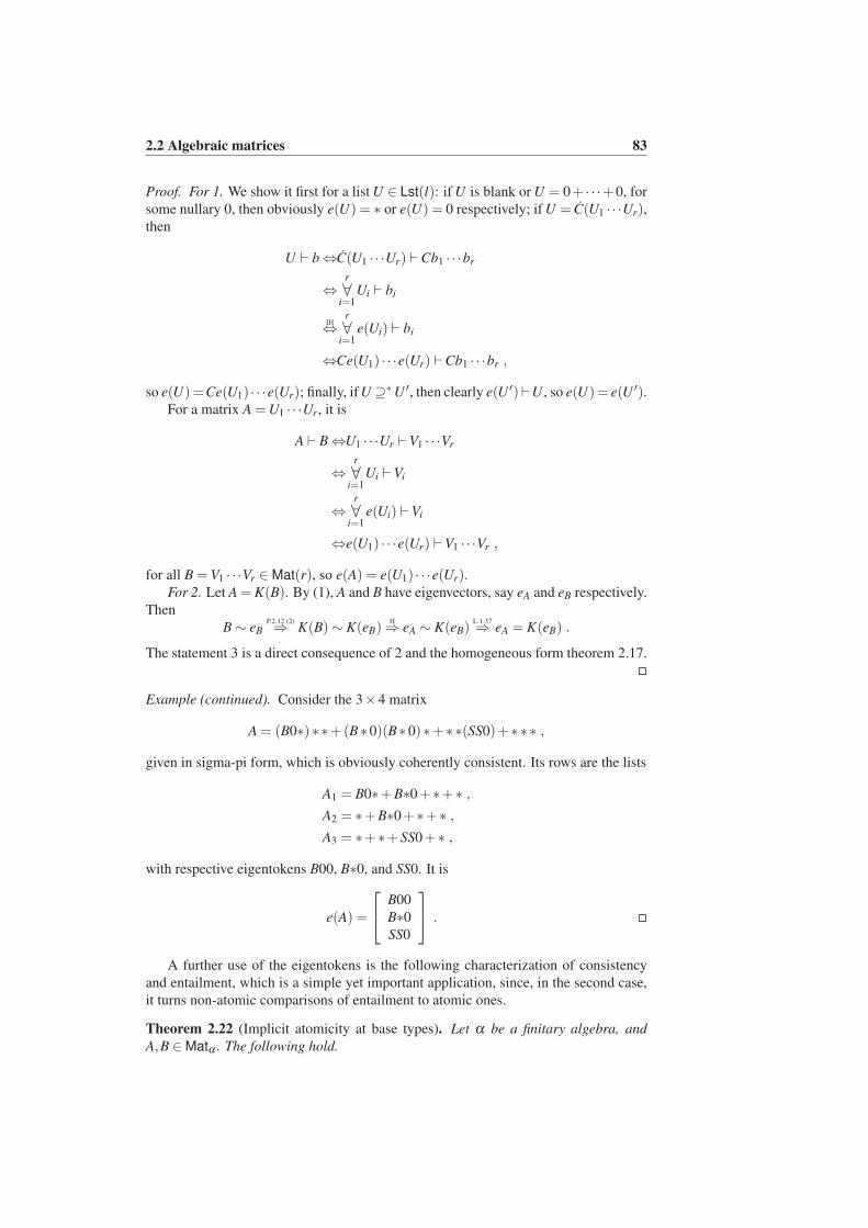
2.2 Algebraic matrices 83
Proof. For 1. We show it first for a list U ∈ Lst(l): if U is blank or U = 0+ · · ·+0, for
some nullary 0, then obviously e(U) = ∗ or e(U) = 0 respectively; if U = C(U1 · · ·Ur),then
U ⊢ b⇔C(U1 · · ·Ur) ⊢Cb1 · · ·br
⇔r
∀i=1
Ui ⊢ bi
IH⇔
r
∀i=1
e(Ui) ⊢ bi
⇔Ce(U1) · · ·e(Ur) ⊢Cb1 · · ·br ,
so e(U)=Ce(U1) · · ·e(Ur); finally, if U ⊇∗U ′, then clearly e(U ′)⊢U , so e(U)= e(U ′).For a matrix A =U1 · · ·Ur, it is
A ⊢ B⇔U1 · · ·Ur ⊢V1 · · ·Vr
⇔r
∀i=1
Ui ⊢Vi
⇔r
∀i=1
e(Ui) ⊢Vi
⇔e(U1) · · ·e(Ur) ⊢V1 · · ·Vr ,
for all B =V1 · · ·Vr ∈Mat(r), so e(A) = e(U1) · · ·e(Ur).For 2. Let A = K(B). By (1), A and B have eigenvectors, say eA and eB respectively.
Then
B∼ eBP.2.12 (2)⇒ K(B)∼ K(eB)
H⇒ eA ∼ K(eB)
L.1.37⇒ eA = K(eB) .
The statement 3 is a direct consequence of 2 and the homogeneous form theorem 2.17.
Example (continued). Consider the 3×4 matrix
A = (B0∗)∗∗+(B∗0)(B∗0)∗+∗∗(SS0)+∗∗∗ ,
given in sigma-pi form, which is obviously coherently consistent. Its rows are the lists
A1 = B0∗+B∗0+∗+∗ ,
A2 = ∗+B∗0+∗+∗ ,
A3 = ∗+∗+SS0+∗ ,
with respective eigentokens B00, B∗0, and SS0. It is
e(A) =
B00
B∗0SS0
.
A further use of the eigentokens is the following characterization of consistency
and entailment, which is a simple yet important application, since, in the second case,
it turns non-atomic comparisons of entailment to atomic ones.
Theorem 2.22 (Implicit atomicity at base types). Let α be a finitary algebra, and
A,B ∈Matα . The following hold.
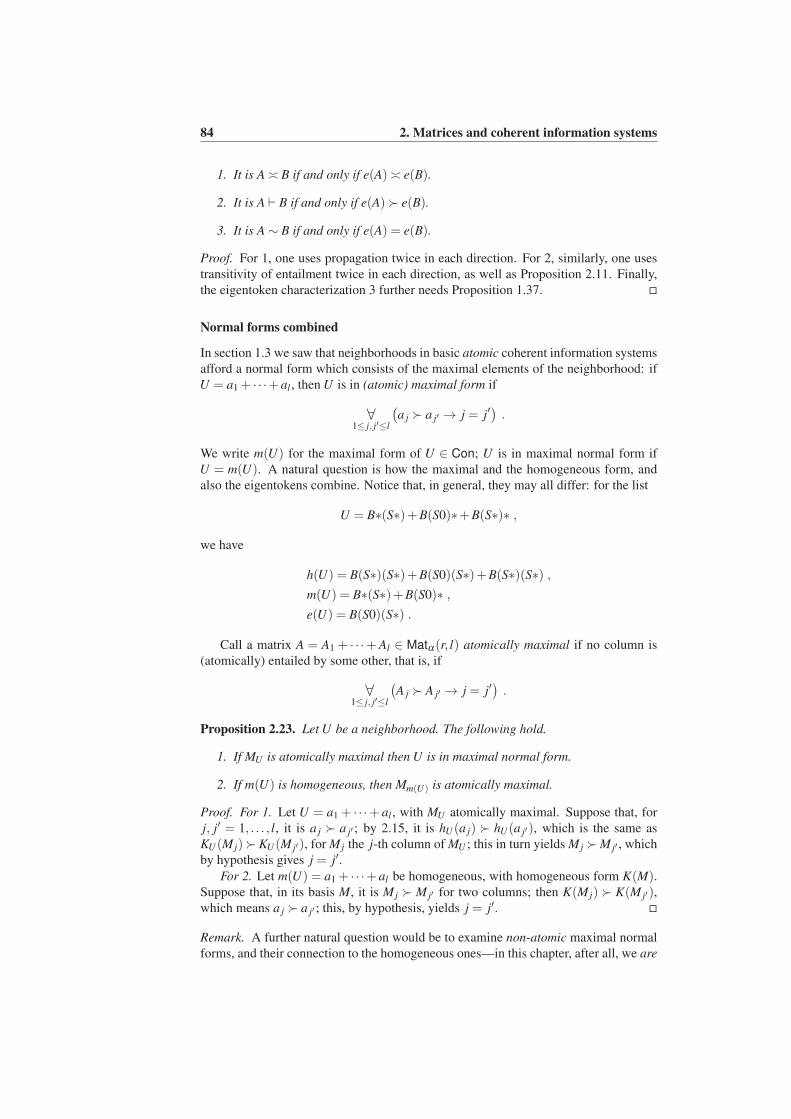
84 2. Matrices and coherent information systems
1. It is A≍ B if and only if e(A)≍ e(B).
2. It is A ⊢ B if and only if e(A)≻ e(B).
3. It is A∼ B if and only if e(A) = e(B).
Proof. For 1, one uses propagation twice in each direction. For 2, similarly, one uses
transitivity of entailment twice in each direction, as well as Proposition 2.11. Finally,
the eigentoken characterization 3 further needs Proposition 1.37.
Normal forms combined
In section 1.3 we saw that neighborhoods in basic atomic coherent information systems
afford a normal form which consists of the maximal elements of the neighborhood: if
U = a1 + · · ·+al , then U is in (atomic) maximal form if
∀1≤ j, j′≤l
(
a j ≻ a j′ → j = j′)
.
We write m(U) for the maximal form of U ∈ Con; U is in maximal normal form if
U = m(U). A natural question is how the maximal and the homogeneous form, and
also the eigentokens combine. Notice that, in general, they may all differ: for the list
U = B∗(S∗)+B(S0)∗+B(S∗)∗ ,
we have
h(U) = B(S∗)(S∗)+B(S0)(S∗)+B(S∗)(S∗) ,
m(U) = B∗(S∗)+B(S0)∗ ,
e(U) = B(S0)(S∗) .
Call a matrix A = A1 + · · ·+Al ∈ Matα(r, l) atomically maximal if no column is
(atomically) entailed by some other, that is, if
∀1≤ j, j′≤l
(
A j ≻ A j′ → j = j′)
.
Proposition 2.23. Let U be a neighborhood. The following hold.
1. If MU is atomically maximal then U is in maximal normal form.
2. If m(U) is homogeneous, then Mm(U) is atomically maximal.
Proof. For 1. Let U = a1 + · · ·+ al , with MU atomically maximal. Suppose that, for
j, j′ = 1, . . . , l, it is a j ≻ a j′ ; by 2.15, it is hU (a j) ≻ hU (a j′), which is the same as
KU (M j)≻ KU (M j′), for M j the j-th column of MU ; this in turn yields M j ≻M j′ , which
by hypothesis gives j = j′.
For 2. Let m(U) = a1 + · · ·+al be homogeneous, with homogeneous form K(M).Suppose that, in its basis M, it is M j ≻ M j′ for two columns; then K(M j) ≻ K(M j′),which means a j ≻ a j′ ; this, by hypothesis, yields j = j′.
Remark. A further natural question would be to examine non-atomic maximal normal
forms, and their connection to the homogeneous ones—in this chapter, after all, we are
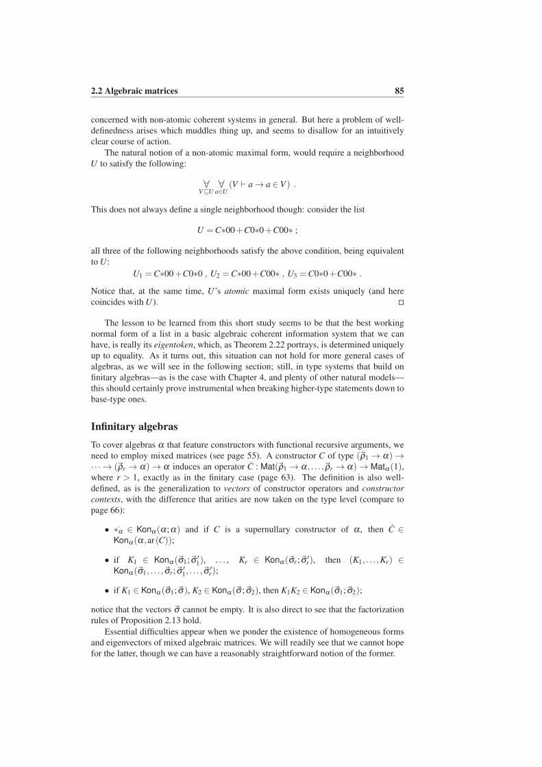
2.2 Algebraic matrices 85
concerned with non-atomic coherent systems in general. But here a problem of well-
definedness arises which muddles thing up, and seems to disallow for an intuitively
clear course of action.
The natural notion of a non-atomic maximal form, would require a neighborhood
U to satisfy the following:
∀V⊆U
∀a∈U
(V ⊢ a→ a ∈V ) .
This does not always define a single neighborhood though: consider the list
U =C∗00+C0∗0+C00∗ ;
all three of the following neighborhoods satisfy the above condition, being equivalent
to U :
U1 =C∗00+C0∗0 , U2 =C∗00+C00∗ , U3 =C0∗0+C00∗ .
Notice that, at the same time, U’s atomic maximal form exists uniquely (and here
coincides with U).
The lesson to be learned from this short study seems to be that the best working
normal form of a list in a basic algebraic coherent information system that we can
have, is really its eigentoken, which, as Theorem 2.22 portrays, is determined uniquely
up to equality. As it turns out, this situation can not hold for more general cases of
algebras, as we will see in the following section; still, in type systems that build on
finitary algebras—as is the case with Chapter 4, and plenty of other natural models—
this should certainly prove instrumental when breaking higher-type statements down to
base-type ones.
Infinitary algebras
To cover algebras α that feature constructors with functional recursive arguments, we
need to employ mixed matrices (see page 55). A constructor C of type (~ρ1 → α)→·· · → (~ρr → α)→ α induces an operator C : Mat(~ρ1 → α, . . . ,~ρr → α)→ Matα(1),where r > 1, exactly as in the finitary case (page 63). The definition is also well-
defined, as is the generalization to vectors of constructor operators and constructor
contexts, with the difference that arities are now taken on the type level (compare to
page 66):
• ∗α ∈ Konα(α;α) and if C is a supernullary constructor of α , then C ∈Konα(α,ar(C));
• if K1 ∈ Konα(~σ1;~σ ′1), . . . , Kr ∈ Konα(~σr;~σ′r), then (K1, . . . ,Kr) ∈
Konα(~σ1, . . . ,~σr;~σ′1, . . . ,~σ
′r);
• if K1 ∈ Konα(~σ1;~σ), K2 ∈ Konα(~σ ;~σ2), then K1K2 ∈ Konα(~σ1;~σ2);
notice that the vectors ~σ cannot be empty. It is also direct to see that the factorization
rules of Proposition 2.13 hold.
Essential difficulties appear when we ponder the existence of homogeneous forms
and eigenvectors of mixed algebraic matrices. We will readily see that we cannot hope
for the latter, though we can have a reasonably straightforward notion of the former.
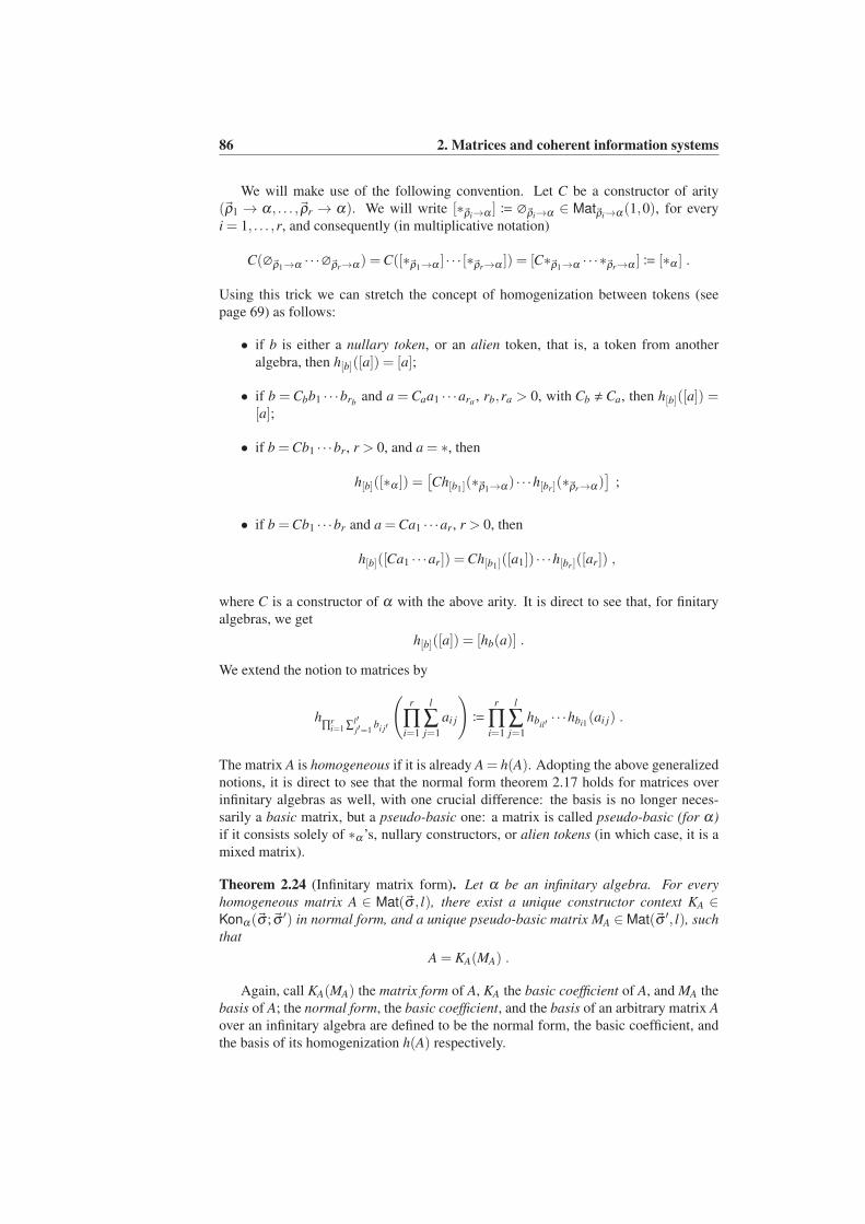
86 2. Matrices and coherent information systems
We will make use of the following convention. Let C be a constructor of arity
(~ρ1 → α, . . . ,~ρr → α). We will write [∗~ρi→α ] ≔ ∅~ρi→α ∈ Mat~ρi→α(1,0), for every
i = 1, . . . ,r, and consequently (in multiplicative notation)
C(∅~ρ1→α · · ·∅~ρr→α) =C([∗~ρ1→α ] · · · [∗~ρr→α ]) = [C∗~ρ1→α · · ·∗~ρr→α ]≔ [∗α ] .
Using this trick we can stretch the concept of homogenization between tokens (see
page 69) as follows:
• if b is either a nullary token, or an alien token, that is, a token from another
algebra, then h[b]([a]) = [a];
• if b = Cbb1 · · ·brband a = Caa1 · · ·ara , rb,ra > 0, with Cb ,Ca, then h[b]([a]) =
[a];
• if b =Cb1 · · ·br, r > 0, and a = ∗, then
h[b]([∗α ]) =[Ch[b1](∗~ρ1→α) · · ·h[br ](∗~ρr→α)
];
• if b =Cb1 · · ·br and a =Ca1 · · ·ar, r > 0, then
h[b]([Ca1 · · ·ar]) =Ch[b1]([a1]) · · ·h[br ]([ar]) ,
where C is a constructor of α with the above arity. It is direct to see that, for finitary
algebras, we get
h[b]([a]) = [hb(a)] .
We extend the notion to matrices by
h∏r
i=1 ∑l′
j′=1bi j′
(r
∏i=1
l
∑j=1
ai j
)
≔
r
∏i=1
l
∑j=1
hbil′· · ·hbi1
(ai j) .
The matrix A is homogeneous if it is already A = h(A). Adopting the above generalized
notions, it is direct to see that the normal form theorem 2.17 holds for matrices over
infinitary algebras as well, with one crucial difference: the basis is no longer neces-
sarily a basic matrix, but a pseudo-basic one: a matrix is called pseudo-basic (for α)
if it consists solely of ∗α ’s, nullary constructors, or alien tokens (in which case, it is a
mixed matrix).
Theorem 2.24 (Infinitary matrix form). Let α be an infinitary algebra. For every
homogeneous matrix A ∈ Mat(~σ , l), there exist a unique constructor context KA ∈Konα(~σ ;~σ ′) in normal form, and a unique pseudo-basic matrix MA ∈Mat(~σ ′, l), such
that
A = KA(MA) .
Again, call KA(MA) the matrix form of A, KA the basic coefficient of A, and MA the
basis of A; the normal form, the basic coefficient, and the basis of an arbitrary matrix A
over an infinitary algebra are defined to be the normal form, the basic coefficient, and
the basis of its homogenization h(A) respectively.
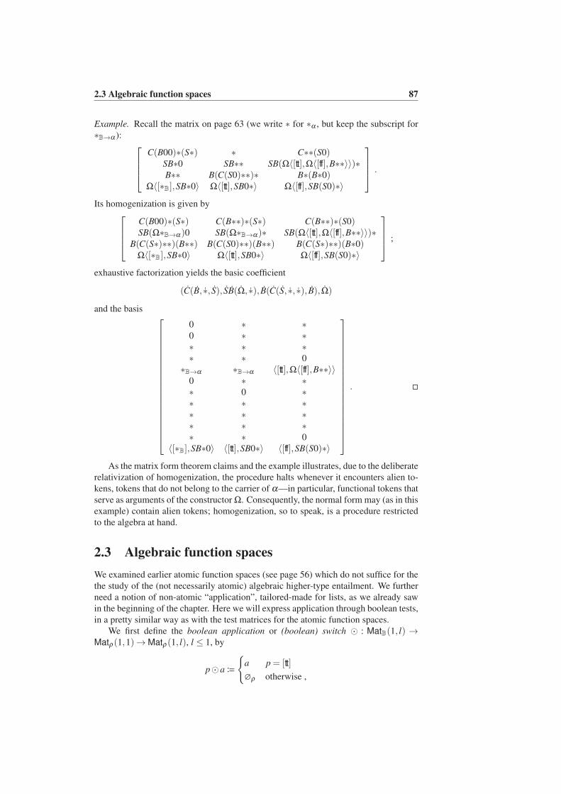
2.3 Algebraic function spaces 87
Example. Recall the matrix on page 63 (we write ∗ for ∗α , but keep the subscript for
∗B→α ):
C(B00)∗(S∗) ∗ C∗∗(S0)SB∗0 SB∗∗ SB(Ω〈[tt],Ω〈[ff],B∗∗〉〉)∗B∗∗ B(C(S0)∗∗)∗ B∗(B∗0)
Ω〈[∗B],SB∗0〉 Ω〈[tt],SB0∗〉 Ω〈[ff],SB(S0)∗〉
.
Its homogenization is given by
C(B00)∗(S∗) C(B∗∗)∗(S∗) C(B∗∗)∗(S0)SB(Ω∗B→α)0 SB(Ω∗B→α)∗ SB(Ω〈[tt],Ω〈[ff],B∗∗〉〉)∗
B(C(S∗)∗∗)(B∗∗) B(C(S0)∗∗)(B∗∗) B(C(S∗)∗∗)(B∗0)Ω〈[∗B],SB∗0〉 Ω〈[tt],SB0∗〉 Ω〈[ff],SB(S0)∗〉
;
exhaustive factorization yields the basic coefficient
(C(B, ∗, S), SB(Ω, ∗), B(C(S, ∗, ∗), B),Ω)
and the basis
0 ∗ ∗0 ∗ ∗∗ ∗ ∗∗ ∗ 0
∗B→α ∗B→α 〈[tt],Ω〈[ff],B∗∗〉〉0 ∗ ∗∗ 0 ∗∗ ∗ ∗∗ ∗ ∗∗ ∗ ∗∗ ∗ 0
〈[∗B],SB∗0〉 〈[tt],SB0∗〉 〈[ff],SB(S0)∗〉
.
As the matrix form theorem claims and the example illustrates, due to the deliberate
relativization of homogenization, the procedure halts whenever it encounters alien to-
kens, tokens that do not belong to the carrier of α—in particular, functional tokens that
serve as arguments of the constructor Ω. Consequently, the normal form may (as in this
example) contain alien tokens; homogenization, so to speak, is a procedure restricted
to the algebra at hand.
2.3 Algebraic function spaces
We examined earlier atomic function spaces (see page 56) which do not suffice for the
the study of the (not necessarily atomic) algebraic higher-type entailment. We further
need a notion of non-atomic “application”, tailored-made for lists, as we already saw
in the beginning of the chapter. Here we will express application through boolean tests,
in a pretty similar way as with the test matrices for the atomic function spaces.
We first define the boolean application or (boolean) switch ⊙ : MatB(1, l) →Matρ(1,1)→Matρ(1, l), l ≤ 1, by
p⊙a≔
a p = [tt]
∅ρ otherwise ,
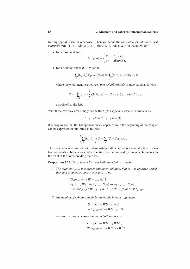
88 2. Matrices and coherent information systems
for any type ρ , basic or otherwise. Then we define the (non-atomic) entailment test
matrix ?⊢: Matρ(1, l)→Matρ(1,1)→MatB(1,1), inductively on the height of ρ:
• for a basic α define
U ?⊢α [a]≔
[tt] U ⊢α a
∅B otherwise;
• for a function space ρ → σ define
∑j
〈U j,b j〉 ?⊢ρ→σ 〈U,b〉≔∑j
(U ?⊢ρ U j)⊙b j?⊢σ b ,
where the entailment test between two neighborhoods is understood as follows:
U ?⊢ρ
l
∑j=1
a j ≔
l⊙
j=1
(U ?⊢ρ a j) = (U ?⊢ρ a1)⊙·· ·⊙ (U ?⊢ρ al) ,
associated to the left.
With these, we may now simply define the higher-type non-atomic entailment by
U ⊢ρ→σ b≔U ?⊢ρ→σ b = [tt] .
It is easy to see that the list application we appealed to in the beginning of the chapter
can be expressed in our terms as follows:
(
∑j
〈U j,b j〉
)
U = ∑j
(U ?⊢U j)⊙b j .
This concludes what we set out to demonstrate: all entailments eventually break down
to entailments in basic acises, which, in turn, are determined by atomic entailments on
the level of the corresponding matrices.
Proposition 2.25. Let ρ and σ be types built upon finitary algebras.
1. The relation ⊢ρ→σ is a proper entailment relation, that is, it is reflexive, transi-
tive, and propagates consistency at ρ → σ :
〈U,b〉 ∈W →W ⊢ρ→σ 〈U,b〉 ,
W1 ⊢ρ→σ W2∧W2 ⊢ρ→σ 〈U,b〉 →W1 ⊢ρ→σ 〈U,b〉 ,
W ∈ Conρ→σ ∧W ⊢ρ→σ 〈U,b〉 →W + 〈U,b〉 ∈ Conρ→σ .
2. Application of neighborhoods is monotonic in both arguments:
U ⊢ρ U ′→WU ⊢σ WU ′ ,
W ⊢ρ→σ W ′→WU ⊢σ W ′U ,
as well as consistency-preserving in both arguments:
U ≍ρ U ′→WU ≍σ WU ′ ,
W ≍ρ→σ W ′→WU ≍σ W ′U .
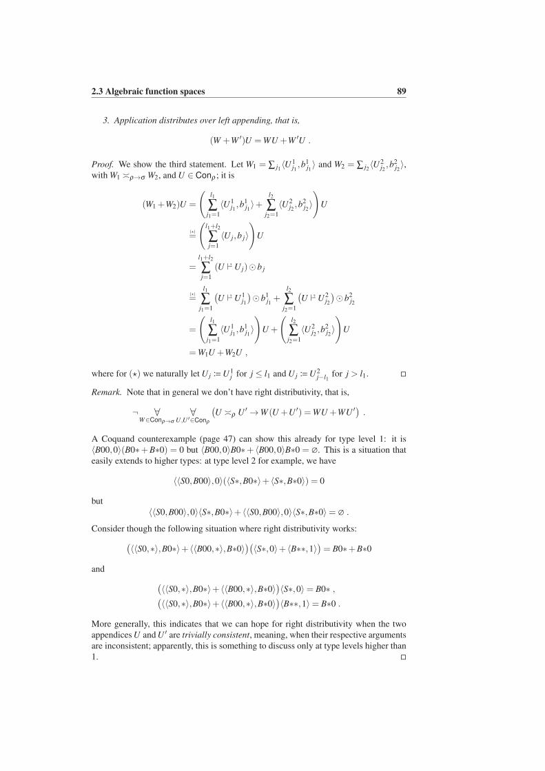
2.3 Algebraic function spaces 89
3. Application distributes over left appending, that is,
(W +W ′)U =WU +W ′U .
Proof. We show the third statement. Let W1 = ∑ j1〈U1
j1,b1
j1〉 and W2 = ∑ j2
〈U2j2,b2
j2〉,
with W1 ≍ρ→σ W2, and U ∈ Conρ ; it is
(W1 +W2)U =
(l1
∑j1=1
〈U1j1,b1
j1〉+
l2
∑j2=1
〈U2j2,b2
j2〉
)
U
(⋆)=
(l1+l2
∑j=1
〈U j,b j〉
)
U
=l1+l2
∑j=1
(U ?⊢U j)⊙b j
(⋆)=
l1
∑j1=1
(
U ?⊢U1j1
)
⊙b1j1+
l2
∑j2=1
(
U ?⊢U2j2
)
⊙b2j2
=
(l1
∑j1=1
〈U1j1,b1
j1〉
)
U +
(l2
∑j2=1
〈U2j2,b2
j2〉
)
U
=W1U +W2U ,
where for (⋆) we naturally let U j ≔U1j for j ≤ l1 and U j ≔U2
j−l1for j > l1.
Remark. Note that in general we don’t have right distributivity, that is,
¬ ∀W∈Conρ→σ
∀U,U ′∈Conρ
(
U ≍ρ U ′→W (U +U ′) =WU +WU ′)
.
A Coquand counterexample (page 47) can show this already for type level 1: it is
〈B00,0〉(B0∗+B∗0) = 0 but 〈B00,0〉B0∗+ 〈B00,0〉B∗0 = ∅. This is a situation that
easily extends to higher types: at type level 2 for example, we have
〈〈S0,B00〉,0〉(〈S∗,B0∗〉+ 〈S∗,B∗0〉) = 0
but
〈〈S0,B00〉,0〉〈S∗,B0∗〉+ 〈〈S0,B00〉,0〉〈S∗,B∗0〉= ∅ .
Consider though the following situation where right distributivity works:
(
〈〈S0,∗〉,B0∗〉+ 〈〈B00,∗〉,B∗0〉)(
〈S∗,0〉+ 〈B∗∗,1〉)
= B0∗+B∗0
and
(
〈〈S0,∗〉,B0∗〉+ 〈〈B00,∗〉,B∗0〉)
〈S∗,0〉= B0∗ ,(
〈〈S0,∗〉,B0∗〉+ 〈〈B00,∗〉,B∗0〉)
〈B∗∗,1〉= B∗0 .
More generally, this indicates that we can hope for right distributivity when the two
appendices U and U ′ are trivially consistent, meaning, when their respective arguments
are inconsistent; apparently, this is something to discuss only at type levels higher than
1.
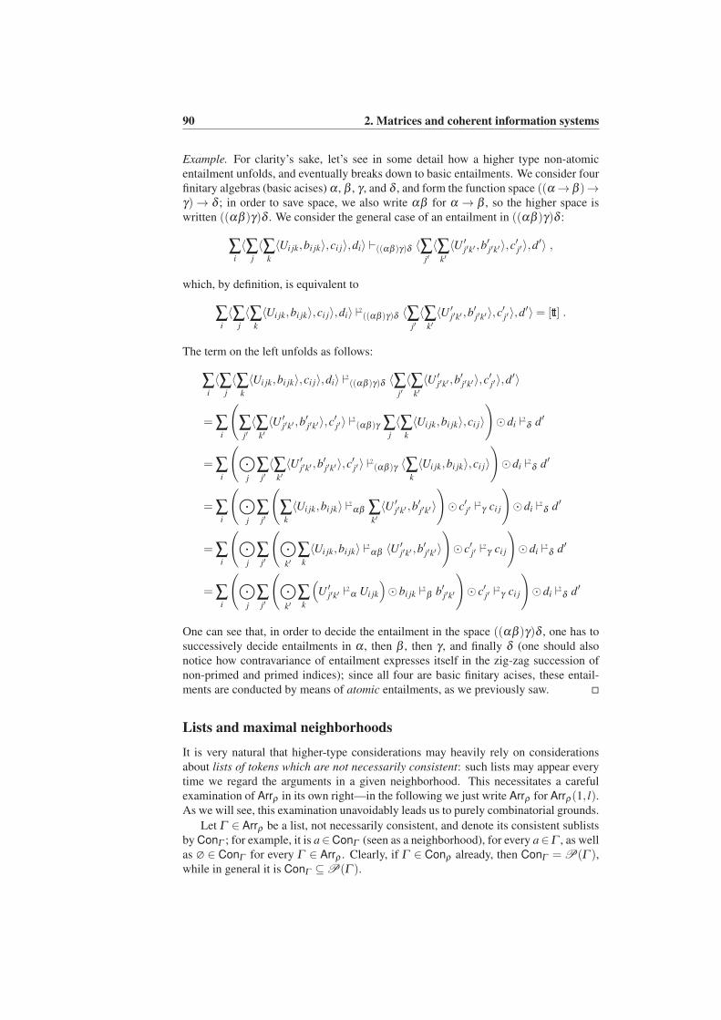
90 2. Matrices and coherent information systems
Example. For clarity’s sake, let’s see in some detail how a higher type non-atomic
entailment unfolds, and eventually breaks down to basic entailments. We consider four
finitary algebras (basic acises) α , β , γ , and δ , and form the function space ((α → β )→γ)→ δ ; in order to save space, we also write αβ for α → β , so the higher space is
written ((αβ )γ)δ . We consider the general case of an entailment in ((αβ )γ)δ :
∑i
〈∑j
〈∑k
〈Ui jk,bi jk〉,ci j〉,di〉 ⊢((αβ )γ)δ 〈∑j′
〈∑k′
〈U ′j′k′ ,b
′j′k′〉,c
′j′〉,d
′〉 ,
which, by definition, is equivalent to
∑i
〈∑j
〈∑k
〈Ui jk,bi jk〉,ci j〉,di〉 ?⊢((αβ )γ)δ 〈∑j′
〈∑k′
〈U ′j′k′ ,b
′j′k′〉,c
′j′〉,d
′〉= [tt] .
The term on the left unfolds as follows:
∑i
〈∑j
〈∑k
〈Ui jk,bi jk〉,ci j〉,di〉 ?⊢((αβ )γ)δ 〈∑j′
〈∑k′
〈U ′j′k′ ,b
′j′k′〉,c
′j′〉,d
′〉
= ∑i
(
∑j′
〈∑k′
〈U ′j′k′ ,b
′j′k′〉,c
′j′〉
?⊢(αβ )γ ∑j
〈∑k
〈Ui jk,bi jk〉,ci j〉
)
⊙di?⊢δ d′
= ∑i
(⊙
j
∑j′
〈∑k′
〈U ′j′k′ ,b
′j′k′〉,c
′j′〉
?⊢(αβ )γ 〈∑k
〈Ui jk,bi jk〉,ci j〉
)
⊙di?⊢δ d′
= ∑i
(⊙
j
∑j′
(
∑k
〈Ui jk,bi jk〉?⊢αβ ∑
k′
〈U ′j′k′ ,b
′j′k′〉
)
⊙ c′j′?⊢γ ci j
)
⊙di?⊢δ d′
= ∑i
(⊙
j
∑j′
(⊙
k′∑k
〈Ui jk,bi jk〉?⊢αβ 〈U
′j′k′ ,b
′j′k′〉
)
⊙ c′j′?⊢γ ci j
)
⊙di?⊢δ d′
= ∑i
(⊙
j
∑j′
(⊙
k′∑k
(
U ′j′k′
?⊢α Ui jk
)
⊙bi jk?⊢β b′j′k′
)
⊙ c′j′?⊢γ ci j
)
⊙di?⊢δ d′
One can see that, in order to decide the entailment in the space ((αβ )γ)δ , one has to
successively decide entailments in α , then β , then γ , and finally δ (one should also
notice how contravariance of entailment expresses itself in the zig-zag succession of
non-primed and primed indices); since all four are basic finitary acises, these entail-
ments are conducted by means of atomic entailments, as we previously saw.
Lists and maximal neighborhoods
It is very natural that higher-type considerations may heavily rely on considerations
about lists of tokens which are not necessarily consistent: such lists may appear every
time we regard the arguments in a given neighborhood. This necessitates a careful
examination of Arrρ in its own right—in the following we just write Arrρ for Arrρ(1, l).As we will see, this examination unavoidably leads us to purely combinatorial grounds.
Let Γ ∈ Arrρ be a list, not necessarily consistent, and denote its consistent sublists
by ConΓ ; for example, it is a∈ConΓ (seen as a neighborhood), for every a∈Γ , as well
as ∅ ∈ ConΓ for every Γ ∈ Arrρ . Clearly, if Γ ∈ Conρ already, then ConΓ = P(Γ ),while in general it is ConΓ ⊆P(Γ ).
2.3 Algebraic function spaces 91
Call M ∈ ConΓ a maximal neighborhood in Γ , and write M ∈MaxΓ , if
∀a∈Γ
(
a≍ρ M → a ∈M)
.
An easy observation is that for all V ∈ Conρ , it is U ⊢ρ V for some U ∈ ConΓ if
and only if M ⊢ρ V for some M ∈ MaxΓ (leftwards let U ≔ M and rightwards use
transitivity of entailment at type ρ).
Moreover, the consistency of a list is characterized easily through maximal neigh-
borhoods: at base types, clearly, a list is consistent if and only if it is its own sole
maximal neighborhood, while for higher types we have the following (recall the defi-
nitions of argA and valA on page 61).
Proposition 2.26. A list Θ ∈ Arrρ→σ is a neighborhood if and only if for each left
maximal M ∈Max(argΘ) there is a right maximal N ∈Max(valΘ) with ΘM ⊆ N.
Proof. Write Γ and ∆ for argΘ and valΘ respectively.
From left to right, let Θ ∈ Conρ→σ and M ∈ MaxΓ . If U,U ′ ∈ M, it will be
U ≍ρ U ′, and then WU ≍σ WU ′; so there must be a maximal N ∈Max∆ with WU ⊆N
for every U ∈Max.
From right to left, let Θ ∈ Arrρ→σ with the property that for each left maximal M ∈MaxΓ there is a right maximal N ∈Max∆ such that ΘM ⊆ N; let 〈U,b〉,〈U ′,b′〉 ∈Θwith U ≍ρ U ′; there will be a maximal M ∈ MaxΓ with U,U ′ ∈ Γ ; by hypothesis,
there will be an N ∈Max∆ such that
b+b′ ⊆WU +WU ′ ⊆ΘW ⊆ N ,
so Θ is consistent.
Write c jΓ (“converging” in Γ ) and d jΓ (“diverging” in Γ ) for the tokens in Γwhich are consistent and inconsistent with its j’th element respectively, that is,
c jΓ ≔ a j′ ∈ Γ | a j ≍ρ a j′ ,
d jΓ ≔ a j′ ∈ Γ | a j 6≍ρ a j′ .
It is obviously Γ = c jΓ +d jΓ , for all j’s.
Proposition 2.27. Let Γ ∈ Arrρ and M ⊆ Γ . It is M ∈MaxΓ if and only if
M =⋂
j∈I(M)
c jΓ .
Proof. From left to right, let M ∈MaxΓ ; it is
ai ∈⋂
j∈I(M)
c jΓ ⇔ ∀j∈I(M)
ai ∈ c jΓ ⇔ ∀j∈I(M)
ai ≍ρ a j(⋆)⇔ ai ∈M ,
where (⋆) holds by the maximality of M.
For the other direction, let M =⋂
j∈I(M) c jΓ ; for the consistency, let ai,a j ∈M, that
is, ai ≍ρ ak and a j ≍ρ ak, for all k ∈ I(M); since i, j ∈ I(M) already, we have ai ≍ρ a j;
for maximality, let ai ≍ρ M, for some i ∈ I(Γ ); then ai ≍ρ a j, for all j ∈ I(M), that is,
ai ∈ c jΓ , for all j ∈ I(M), so ai ∈⋂
j∈I(M) c jΓ , hence ai ∈M by the hypothesis.
92 2. Matrices and coherent information systems
By the graph-theoretic intuition we appealed to in the previous remark, Proposi-
tion 2.27 expresses that a maximal clique is characterized by the intersection of the
stars induced by its nodes.
We are interested in the way maximal neighborhoods form as we move to a higher
type, so that we may in principle argue about lists in a type-inductive fashion. Introduce
the following shorthands for the sake of readability. Given a list Θ ∈ Arrρ→σ , and
M ∈ Conρ , N ∈ Conσ , write 〈M,N〉Θ for all 〈U,b〉 ∈Θ with M ⊢ρ U and N ⊢σ b. If
Γ ∈ Arrρ , and ∆ ∈ Arrσ , then write 〈Γ ,∆〉 for ∑M∈MaxΓ ∑b∈∆ 〈M,b〉.
Proposition 2.28. Let Θ ∈ Arrρ→σ . The following hold.
1. c jΘ = 〈d jargΘ ,valΘ〉Θ ∪〈argΘ ,c jvalΘ〉Θ ,
2. d jΘ = 〈c jargΘ ,valΘ〉Θ ∩〈argΘ ,d jvalΘ〉Θ .
Proof. For 1:
〈U j′ ,b j′〉 ∈ c jΘ ⇔U j 6≍ρ U j′ ∨b j ≍σ b j′
⇔U j′ ∈ d jargΘ ∨b j′ ∈ c jvalΘ
⇔ 〈U j,b j〉 ∈ 〈d jargΘ ,valΘ〉Θ ∪〈argΘ ,c jvalΘ〉Θ .
Statement 2 is shown similarly:
〈U j′ ,b j′〉 ∈ d jΘ ⇔U j ≍ρ U j′ ∧b j 6≍σ b j′
⇔U j′ ∈ c jargΘ ∧b j′ ∈ d jvalΘ
⇔ 〈U j,b j〉 ∈ 〈c jargΘ ,valΘ〉Θ ∩〈argΘ ,d jvalΘ〉Θ .
The following is a characterization of higher-type maximal neighborhoods.
Proposition 2.29. Let Θ ∈ Arrρ→σ and P⊆Θ . It is P ∈MaxΘ if and only if
P =⋃
K⊆I(P)
⋂
k∈K
〈dkargΘ ,valΘ〉Θ ∩⋂
k∈I(P)rK
〈argΘ ,ckvalΘ〉Θ
.
Proof. Let Θ ∈ Arrρ→σ , and write Γ ≔ argΘ , ∆ ≔ valΘ . By Proposition 2.27 we
know that P ∈MaxΘ if and only if
P =⋂
j∈I(P)
c jΘP. 2.28=
⋂
j∈I(P)
(〈d jΓ ,∆〉Θ ∪〈Γ ,c j∆〉Θ ) ,
so we want to show that the following equation holds:
⋂
j∈I(P)
(〈d jΓ ,∆〉Θ ∪〈Γ ,c j∆〉Θ )
=⋃
K⊆I(P)
⋂
k∈K
〈dkΓ ,∆〉Θ ∩⋂
k∈I(P)rK
〈Γ ,ck∆〉Θ
.
(2.24)
We relax the notation even more by writing d j for 〈d jΓ ,∆〉Θ and c j for 〈Γ ,c j∆〉Θ , so
the equation (2.24) becomes
⋂
j∈I(P)
(d j ∪ c j) =⋃
K⊆I(P)
⋂
k∈K
dk ∩⋂
k∈I(P)rK
ck
.
2.3 Algebraic function spaces 93
We show that the equation holds by induction on n = |I(P)|> 0. The base case is direct
to see. Let I(P) = 1, . . . ,n,n+1; then
n+1⋂
j=1
(d j ∪ c j) =n⋂
j=1
(d j ∪ c j)∩ (dn+1∪ cn+1)
(IH)=
⋃
K⊆1,...,n
(⋂
k∈K
dk ∩⋂
k<K
ck
)
∩ (dn+1∪ cn+1)
=⋃
K⊆1,...,n
(⋂
k∈K
dk ∩⋂
k<K
ck ∩dn+1
)
∪⋃
K⊆1,...,n
(⋂
k∈K
dk ∩⋂
k<K
ck ∩ cn+1
)
=⋃
K⊆1,...,n+1
(⋂
k∈K
dk ∩⋂
k<K
ck
)
,
where the last steps require careful but elementary set theory.
Remark. Note that in the proof we have used the following convention: if Θ ∈ Arrρ→σ
and Q ⊆Θ , indexed by I(Q), then⋂
k∈∅Q(k) = Θ (“an intersection over the empty
index set yields the universe”).
We need to be a bit careful with the way we use the lists of arguments in given
neighborhoods: do we mean them as lists of neighborhoods, that is, lists of type Nρ , or
as lists of the neighborhoods’ tokens, that is, lists of type ρ? For our purposes, it turns
out that, given a list in Nρ , we can work with its underlying “flat” list in ρ , and then
draw safe conclusions about it in Nρ again.
Define a flattening mapping fl : ArrNρ → Arrρ in the usual way:
fl(Γ )≔ ∑U∈Γ
∑a∈U
a ;
in set-theoretical notation we may as well write fl(Γ ) = ∪Γ (we return to this in Chap-
ter 3, on page 108).
Proposition 2.30. Let Γ ∈ ArrNρ . Then
∀M∈MaxΓ
∃!M f∈Maxfl(Γ )
M f ⊢Nρ M ∧ ∀M f∈Maxfl(Γ )
∃!M∈MaxΓ
M f ⊢Nρ M .
Proof. Let Γ ∈ ArrNρ . For the first conjunct, let M ∈MaxΓ ; it is consistent, so U ≍Nρ
U ′, for all U ∈ M, which means that a ≍ρ a′, for all a ∈U , a′ ∈U ′; then there must
exist a maximal neighborhood M f in fl(Γ ), which will contain all a∈U , for any U ∈M,
so M f ⊢Nρ M. Suppose that M′f is yet another maximal neighborhood in fl(Γ ), with
M′f ⊢Nρ M; then, since entailment preserves consistency, for all a ∈ fl(Γ ) it is
[a]≍Nρ M → a≍ρ M f ∧a≍ρ M′f ,
which yields M f = M′f due to their maximality with respect to consistency.
For the second conjunct, let M f ∈Maxfl(Γ ); since the situation is finite, we may
argue indirectly; let M1, . . . ,MT be all maximals in Γ , and suppose that M f 0Nρ Mt
for any t = 1, . . . ,T ; by the first conjunct, there is an Mtf ∈Maxfl(Γ ), with Mt
f ⊢Mt ,
for every t, and since Mt ’s together cover Γ , their corresponding Mtf ’s together must
cover fl(Γ ); on the other hand, the supposition yields M f 6≍ρ Mtf , for all t, which would
mean that there are a ∈M f rfl(Γ ), a contradiction. Assume now that M f ⊢Nρ M and
M f ⊢Nρ M′, for M,M′ ∈MaxΓ ; then M ≍Nρ M′, so M = M′ by maximality.
94 2. Matrices and coherent information systems
Eigen-neighborhoods
Let Γ ∈ Arrρ be an arbitrary list. In the following we drop the maximality requirement
of the previous section and consider arbitrary neighborhoods U ⊆ Γ which are still
“closed under entailment relatively to Γ ”, in a way that we describe below.
Let W ∈ Conρ→σ be some neighborhood, and consider a sublist E ⊆W which has
the property
U1 ≍ρ U2∧b1 ≍σ b2 ,
for all 〈Ui,bi〉 ∈ E, i = 1,2. Suppose further that all these arguments U in E are part of
an ideal x ∈ Ideρ ; then b ∈W (x), for all the corresponding values b in E. Conversely,
if such an ideal x entails exactly argE out of all arguments of W—in which case, due to
closure of x, argE would already contain all of argW that it entails—then the elicited
value should be exactly valE; in other words, this sub-neighborhood would serve as a
pointer to all ideals like x extending its argument exclusively in W , while simultane-
ously providing the exact value that W would give out as a result by application. Let’s
try and flesh out this intuition.
Call a sublist E ⊆W an eigen-neighborhood of W , and write E ∈ EigW , if it is
left-consistent, that is,
∀U1,U2∈argE
U1 ≍ρ U2
(so consequently b1 ≍σ b2 for the corresponding arguments as well), and left-closed
under entailment relatively to W , that is,
∀〈U,b〉∈W
(
argE ⊢Nρ U → 〈U,b〉 ∈ E)
,
where Nρ is the corresponding information system of the neighborhoods of ρ5. Every
U ∈ argW generates an eigen-neighborhood EU of W , by
〈U ′,b〉 ∈ EU ≔ 〈U′,b〉 ∈W ∧U ⊢ρ U ′ .
Furthermore, it is clear that W ∼ρ→σ ∑E∈EigW E.
This is not an inductively defined concept, but merely focuses on the arguments of
the higher-type neighborhood at hand. Still, we can conventionally define the eigen-
neighborhoods of a base-type neighborhood U ∈ Conα to be U itself and ∅α .
Remark. For some intuition on this convention one can think of every base type α as
being isomorphic to the function space U→ α , where U is the unit type. Otherwise,
one can quite easily see that the set of eigen-neighborhoods of a given neighborhood
can indeed be defined inductively. This leads to a method of inductive proof that we
implicitly use in section 2.4.
The eigen-neighborhoods behave as generalized tokens to some extent, enough to
reveal a quite unexpected atomic behavior that underlies the otherwise non-atomic al-
gebraic entailment.
5The neighborhood information system of ρ is the triple Nρ = (Conρ ,ConNρ ,⊢Nρ ), where ∑lj=1 U j ∈
ConNρ if and only if ∪lj=1U j ∈Conρ and ∑
lj=1 U j ⊢Nρ U if and only if ∪l
j=1U j ⊢ρ U . This is an information
system which is coherent if ρ is coherent and moreover the two have isomorphic domains of ideals (see
Chapter 3, page 108).
2.3 Algebraic function spaces 95
Theorem 2.31 (Implicit atomicity at higher types). Let W1,W2 ∈Conρ→σ . The follow-
ing hold:
W1 ≍ρ→σ W2 ↔ ∀E1∈EigW1
∀E2∈EigW2
(
argE1 ≍Nρ argE2 → valE1 ≍σ valE2
)
,
W1 ⊢ρ→σ W2 ↔ ∀E2∈EigW2
∃E1∈EigW1
(
argE2 ⊢Nρ argE1∧valE1 ⊢σ valE2
)
.
Proof. Let W1,W2 ∈ Conρ→σ . For consistency, let first W1 ≍ρ→σ W2 and Ei ∈ EigWi,
i = 1,2, with argE1 ≍Nρ argE2; the latter means U1 ≍ρ U2, for any Ui ∈ argEi, which
by the consistency of W yields b1 ≍σ b2, for any bi ∈ valEi. Conversely, let
argE1 ≍Nρ argE2 → valE1 ≍σ valE2 ,
for all Ei ∈ EigWi, i = 1,2, and 〈Ui,bi〉 ∈ Wi with U1 ≍ρ U2; let EUibe the
eigen-neighborhood in Wi generated by Ui; by the propagation of consistency, it is
argEU1≍Nρ argEU2
, so the assumption yields b1 ∈ valEU1≍σ valEU1
∋ b2.
For entailment, it is:
W1 ⊢ρ→σ W2 ⇔ ∀E2∈EigW2
W1 ⊢ρ→σ E2
⇔ ∀E2∈EigW2
W1argE2 ⊢σ valE2
⇔ ∀E2∈EigW2
∃〈U1,b1〉,...,〈Ul ,bl〉∈W1
(l
∀j=1
argE2 ⊢ρ Ul ∧l
∑j=1
b j ⊢σ valE2
)
(⋆)⇔ ∀
E2∈EigW2
∃E1∈EigW1
(
argE2 ⊢Nρ argE1∧valE1 ⊢σ valE2
)
,
where (⋆) holds by setting 〈U,b〉 ∈ E1 for some 〈U,b〉 ∈W1, whenever ∑lj=1 U j ⊢ρ U ;
that this is indeed an eigen-neighborhood of W1 follows directly by the propagation of
consistency and transitivity of entailment at ρ .
Write 〈U,V 〉 for ∑b∈V 〈U,b〉 and U ∼ρ U ′ for U ⊢ρ U ′ ∧U ′ ⊢ρ U (equientailment
is clearly an equivalence on neighborhoods). With the use of eigen-neighborhoods we
can achieve manageable conservative extensions of a neighborhood.
Proposition 2.32. Let W ∈ Conρ→σ , and E1, . . . ,Em ∈ EigW. For any choice of
U1, . . . ,Um ∈ Conρ and V1, . . . ,Vm ∈ Conσ with the property that Ui ⊢ρ argEi and
valEi ⊢σ Vi, for i = 1, . . . ,m, it is
W ∼ρ→σ W +m
∑i=1
〈Ui,Vi〉 .
Proof. For the consistency of the extension W +∑mi=1〈Ui,Vi〉, let i, j = 1, . . . ,m; then
Ui ≍ρ U j ⇒ argEi ≍ρ argE j ⇒ valEi ≍σ valE j ⇒Vi ≍σ Vj ,
by the propagation of consistency and consistency of W ; this suffices.
For the equientailment, let i = 1, . . . ,m; it is
Ui ⊢Nρ argEi∧valEi ⊢σ Vi ⇒ Ei ⊢ρ→σ 〈Ui,Vi〉 ,
so W ⊢ρ→σ W +∑mi=1〈Ui,Vi〉. The converse is trivial.
96 2. Matrices and coherent information systems
For every E ∈ EigW there is exactly one UE ∈ Conρ (up to equientailment) and
exactly one V E ∈ Conσ (up to equientailment), such that E ∼ρ→σ 〈UE ,V E〉; just set
UE≔ fl(argE) and V E
≔ valE
(for the definition of the flattening mapping see page 93). Say that W is in eigenform,
if for every E ∈ EigW it is 〈UE ,V E〉 ⊆W . Furthermore call W monotone, if for all
〈U1,V1〉,〈U2,V2〉 ⊆W it is
U1 ⊢ρ U2 →V1 ⊢σ V2 .
For example, 〈S0,B01〉+ 〈S∗,B∗1〉 is monotone whereas 〈S0,B∗1〉+ 〈S∗,B01〉 isn’t.
Proposition 2.33. Let ρ , σ be types. For all W ∈ Conρ→σ , there is a monotone W ′ ∈Conρ→σ in eigenform, such that W ∼ρ→σ W ′.
Proof. Let W ∈ Conρ→σ . Set Γ ≔ fl(argW ), and
W ′≔ ∑
U∈ConΓ
〈U,WU〉 .
It is easy to see that this list is finite and consistent; that it is monotone follows from
the monotonicity of application; that it is in eigenform is obvious by construction.
We show the equientailment. Let 〈U,b〉 ∈W ; since obviously U ∈ ConΓ and b ∈WU , it is immediate that W ′ ⊢ρ→σ W . For the other direction, let 〈U,V 〉 ⊆W ′, for
some U ∈ConΓ ; since obviously WU ⊢σ WU , the definition of higher-type entailment
immediately yields W ⊢ρ→σ 〈U,WU〉.
So the non-monotone neighborhood 〈S0,B∗1〉+〈S∗,B01〉 has the equivalent mono-
tone eigenform
〈∅,∅〉+ 〈S0,B∗1+B01〉+ 〈S∗,B01〉+ 〈S0+S∗,B∗1+B01〉 ,
or, written in tokens,
〈S0,B∗1〉+ 〈S0,B01〉+ 〈S∗,B01〉+ 〈S0+S∗,B∗1〉+ 〈S0+S∗,B01〉 .
Now let Θ ∈ Arrρ→σ . We can use eigen-neighborhoods to define an eigensplitting
mapping sp : Arrρ→σ → Arrρ→σ by
spΘ ≔ ∑〈U,b〉∈Θ
∑E∈EigU
〈E,b〉 ,
such that it commutes with the flattening mapping.
Proposition 2.34. Let W1 +N · · ·+N WJ ∈ ArrN(ρ→σ). Then
sp(fl(W1 +N · · ·+N WJ)) = fl(spW1 +N · · ·+N spWJ) .
Proof. It is
sp(fl(W1 +N · · ·+N WJ)) = sp(W1 + · · ·+WJ)(⋆)= sp(W1)+ · · ·+ sp(WJ)
= fl(sp(W1)+N · · ·+N sp(WJ)) ,
where (⋆) is direct to see from the definition of eigensplitting.
2.4 Totality and density 97
2.4 Totality and density
In a finitary basic algebraic coherent information system a token is total when it in-
volves no stars, and a neighborhood is total when it entails a total token; write GT and
GCon for total tokens and total neighborhoods respectively. Define the total ideals at
type ρ , and write Gρ , by the following: at base type α , x is total if it contains a total
token; at type ρ → σ , f is total when, applied to a total ideal, it yields a total ideal, that
is, when
∀x∈ρ
(
x ∈ Gρ → f (x) ∈ Gσ
)
,
where b∈ f (x) if and only if 〈U,b〉 ∈ f , for some U ⊆ x. A type ρ is called dense when
every neighborhood U ∈ Conρ can be extended to a total ideal x ∈ Gρ . The last main
result of this chapter is the density theorem (Theorem 2.37), which states that every
type is dense.
At every base type α we demand the existence of a distinguished nullary construc-
tor 0α . Noting that every type ρ has the form ρ1 → ·· · → ρp → α , for some base type
α and some non-negative number p, write ρ− for the (possibly empty) finite sequence
(ρ1, . . . ,ρp) of the argument types, and Conρ− for Conρ1× ·· ·×Conρp ; elements of
Conρ− are (possibly empty) finite sequences of neighborhoods of the corresponding
types.
Lemma 2.35 (Separation). Let ρ be a type. For every U1,U2 ∈Conρ , if U1 6≍ρ U2 then
there exists a separator U− ∈ Conρ− such that U1U− 6≍α U2U−.
Proof by induction on types. At a base type there is nothing to show. Let W1,W2 ∈Conρ→σ , with W1 6≍ρ→σ W2. There will be 〈Ui,bi〉 ∈Wi, i = 1,2, with 〈U1,b1〉 6≍ρ→σ
〈U2,b2〉, that is, with U1 ≍ρ U2 ∧ b1 6≍σ b2. By the induction hypothesis, there is a
separator of b1, b2, that is, a finite sequence V− ∈ Conσ− such that b1V− 6≍α b2V−.
Set U−≔ (U1+U2,V
−); this is obviously a finite sequence in Con(ρ→σ)− and satisfies
what we need.
Remark. Notice that the choice of U− in the proof is not unique, since there may be
more than one inconsistency between W1 and W2.
Now we state another useful lemma without proof (see [49, §6.5]).
Lemma 2.36 (Extension). Let ρ be a type and f ,g ∈ Ideρ . If f ∈ Gρ and f ⊆ g then
g ∈ Gρ .
Theorem 2.37 (Density). Let ρ be a type. For every U ∈ Conρ there is an x ∈ Ideρ ,
such that U ⊆ x and x ∈ Gρ .
Proof by induction on types. At base type α , let U ∈Conα , and b≔ e(U) be its eigen-
token. Clearly, it suffices to find a total token a ∈ GTα with a ⊢α b, and then set
x≔ a. If b = 0, for some nullary constructor 0, then set a≔ b; if b = ∗α , set a≔ 0α .
If b = Cb1 · · ·br, then the induction hypothesis gives ai ∈ GTα , with ai ⊢α bi, for
i = 1, . . . ,r, so setting a≔Ca1 · · ·ar ∈ GTα gives a ⊢α b.
At type ρ → σ , assume that σ and all types in ρ− are dense. Let W = ∑nk=1〈Uk,bk〉
be a neighborhood. Observe first that, if there are indices i, j = 1, . . . ,n such that bi 6≍σ
b j, then it is also Ui 6≍ρ U j, by the consistency of W . Then by Lemma 2.35 there is a
separator U−i j ∈ Conρ− of Ui, U j. In the following we assume that U−
i j =U−ji .
98 2. Matrices and coherent information systems
For an arbitrary neighborhood U ∈ Conρ gather its fitting values in W , if any, by
VU ≔ bk |n
∀i=1
(
bi 6≍σ bk →UU−ik ⊢α UkU
−ik
)
;
notice that bk ∈VUk. This is a neighborhood: let bi,b j ∈VU , and suppose that bi 6≍σ b j;
by the definition of VU it is
UU−i j ⊢α UiU
−i j ∧ UU−
i j ⊢α U jU−i j ⇒UiU
−i j ≍α U jU
−i j ,
which contradicts that U−i j is a separator. Moreover, it is monotone in U : let U,U ′ ∈
Conρ , with U ⊢ρ U ′; by monotonicity of application it is UU−ik ⊢α U ′U−
ik ; by the defi-
nition of VU , it is direct to check that, if bk ∈ VU ′ , then bk ∈ VU as well, so the desired
monotonicity follows trivially by inclusion.
By the induction hypothesis we have density at type σ , so VU will have a total
extension vU . Set
f ≔ 〈U,b〉 |
(
∀1≤i, j≤n
(
bi 6≍σ b j →UU−i j ∈ GConα
)
∧b ∈ vU
)
∨VU ⊢σ b . (2.25)
Since bk ∈ VUk, it is clear that f contains W . We show that f is an ideal, by showing
that it is an approximable mapping.
First, it is consistently defined: Let 〈U,V 〉 ⊆ f ; we show that V ∈ Conσ . For
arbitrary b,b′ ∈V , by the definition of f , it is either b,b′ ∈ vU , or b ∈ vU ∧VU ⊢ b′, or
VU ⊢ b,b′, so b≍σ b′ in all three cases.
Then, it is deductively closed on the right: Let 〈U,V 〉 ⊆ f and V ⊢σ b; we show
that 〈U,b〉 ∈ f . There are two cases: either b′ ∈ vU , for some b′ ∈ V , or VU ⊢σ b′, for
all b′ ∈V . In the first case, we have V ⊆ vU , and since vU is deductively closed, b∈ vU .
In the second case, we have VU ⊢σ b by transitivity at σ .
Finally, it is deductively closed on the left: Let U ⊢ρ U ′ and 〈U ′,b〉 ∈ f ; we show
that 〈U,b〉 ∈ f . In case U ′U−i j ∈ GConα , for bi 6≍σ b j, by monotonicity of application
it is also UU−i j ∈ GConα . Moreover, since U ⊢ρ U ′, both U ′U−
i j and U ′U−i j will entail
the same total token, so VU =VU ′ , and then b ∈ vU . In case VU ′ ⊢σ b, monotonicity of
VU in U yields VU ⊢ b.
It remains to show totality. Let x ∈ Gρ . We show that f (x) ∈ Gσ . By the definition
of application we have
b ∈ f (x)⇔ ∃U⊆x〈U,b〉 ∈ f .
For all i, j = 1, . . . ,n with bi 6≍σ b j we have separators U−i j ∈ Conρ− ; by the induction
hypotheses at types in ρ−, for every such separator there exists a finite sequence u−i j
of corresponding total extensions. By totality of x we have x(u−i j) ∈ Gα . Let U be
the union of all Ui j ⊆ x with Ui ju−i j ∈ GConα ; it is also Uu−i j ∈ GConα . Then, for all
b ∈ vU , it is 〈U,b〉 ∈ f , which means that vU ⊆ f (x). By Lemma 2.36 we have that
f (x) ∈ Gσ .
Now let us examine what it means for our setting that the density statement holds.
Write x≍ρ U if Ux ≍ρ U for all Ux ⊆ x.
Proposition 2.38. For all x ∈ Gρ and U ∈ Conρ it is effectively either x ≍ρ U or
x 6≍ρ U.
2.4 Totality and density 99
Proof by induction on types. At base type α , let x ∈ Gα and U ∈ Conα ; let a ∈ x be
the total token of x; then either a≍α U or a 6≍α U , so either x≍α U or x 6≍α U .
At type ρ → σ , let f ∈ Gρ→σ and W ∈ Conρ→σ ; let 〈U,V 〉 ∈ Eig(W ); by The-
orem 2.37 there exists an x ∈ Gρ with U ⊆ x; f is total, so f (x) ∈ Gσ , and it is ei-
ther f (x) ≍σ V or f (x) 6≍σ V by the induction hypothesis at σ ; so we can decide if
f ≍ρ→σ 〈U,V 〉 holds for all eigen-neighborhoods of W or if f 6≍ρ→σ 〈U,V 〉 for some
of them; in the first case we have f ≍ρ→σ W , and in the second we have f 6≍ρ→σ W .
Note that there is a neighborhood at each type ρ , which is consistent with all total
ideals, namely ∅ρ , the empty one. Now suppose that we are given the list of argu-
ments of some higher-type neighborhood, and that it contains two inconsistent neigh-
borhoods; the following implies that we can witness their inconsistency in a minimal
way.
Proposition 2.39. For all x ∈ Gρ and U1,U2 ∈ Conρ in eigenform, if x ≍ρ U1 and
U1 6≍ρ U2 then
1. x 6≍ρ U2, and furthermore,
2. there is a Ux,1 ∈ Conρ , such that U1 ⊢ρ Ux,1 ⊆ x and Ux,1 6≍ρ U2.
Proof by induction on types. At type α , let x ∈ Gα and U1,U2 ∈ Conα , with x ≍α U1
and U1 6≍α U2; then U1⊆ x, and the second assumption yields x 6≍α U2, so the property 1
holds. The property 2 holds as well, for Ux,1≔U1.
At type ρ → σ , let f ∈ Gρ→σ and W1,W2 ∈ Conρ→σ , with f ≍ρ→σ W1 and
W1 6≍ρ→σ W2; by Theorem 2.31 and the fact that the neighborhoods are in eigenform,
there will be 〈Ui,Vi〉 ⊆Wi, i = 1,2, such that
〈U1,V1〉 6≍ρ→σ 〈U2,V2〉 ,
which means
U1 ≍ρ U2∧V1 6≍σ V2 ;
by Theorem 2.37 there is an x ∈ Gρ with U1 +U2 ⊆ x, and by the totality of f we have
f (x) ∈ Gσ , for which
f (x)≍σ V1∧V1 6≍σ V2 .
The induction hypothesis that 1 holds at σ yields f (x) 6≍σ V2, so f 6≍ρ→σ 〈U2,V2〉, and
consequently f 6≍ρ→σ W2, so the property 1 holds at ρ → σ as well.
The induction hypothesis that 2 holds at σ yields a V f (x),1 ∈ Conσ , with
V1 ⊢σ V f (x),1 ⊆ f (x) ∧ V f (x),1 6≍σ V2 ;
by the definition of application of ideals, let U f (x),1 ∈ Conρ be an argument for V f (x),1
in f , that is, be such that
〈U f (x),1,V f (x),1〉 ⊆ f ∧ U f (x),1 ⊆ x ;
then 〈U f (x),1 +U1 +U2,Vf (x),1〉 ⊆ f , by the deductive closure of f ; it is
〈U1,V1〉 ⊢ρ→σ 〈Uf (x),1 +U1 +U2,V
f (x),1〉 ⊆ f ,
and
〈U f (x),1 +U1 +U2,Vf (x),1〉 6≍ρ→σ 〈U2,V2〉 ;
100 2. Matrices and coherent information systems
so it suffices to set
W f ,1≔ ∑
U1∈Confl(argW1)
〈U f (x),1 +U1 +U2,Vf (x),1〉 ,
and the property 2 holds at ρ → σ as well.
2.5 Notes
Non-blank-row matrices
Proposition 2.6 interestingly implies that matrices with non-blank rows together with
matrix overlapping and matrix inclusion form an acis; let us call this nbr-acis and
denote it by (Arrnbr,≬,⊂). This acis is different from the (Mat,≍,≻), since the carriers
are clearly distinct: blank arrays belong to Mat but not to Arrnbr and the former contains
only coherently consistent matrices. However, one can easily show that if A ⊂ B then
B≻ A, though no similar remark can be made for ≬ and ≍.
This last remark is nevertheless misleading as far as the nature of this structure
is concerned. The nbr-acis essentially mimics the conjunction-implication systems of
page 51: given two (decidable) formulas, suppose we induce corresponding matrices
(like the test matrices we used for the function spaces); then overlapping of the latter
mimics the conjunction of the former while inclusion of the latter mimics implication
of the former, as is portrayed by Theorem 2.8.
On normal forms
The notion of a “normal form”, as is well known, is a prime player in the context of
rewriting systems (see for example [54]). A rewriting system is just a set A with a
binary relation→, its rewrite relation. We say that an element a ∈ A is in normal form
if it is not further rewritable, that is, if there is no b ∈ A for which a→ b. The rewriting
system is uniquely normalizing if for every a ∈ A there is a unique normal form a′ ∈ A
such that a→⋆ a′ (→⋆ being the reflexive-transitive closure of→); we say that a′ is the
normal form of a.
Under this terminology, there are three different notions of normal forms of a
given neighborhood U that we have encountered: the maximal form m(U) (pages 33
and 84), the homogeneous form h(U) (page 69) and the eigentoken, or eigenform,
e(U) (page 82). As we have seen, the only ubiquitous one is the homogeneous form,
as it makes sense for all finitary and infinitary algebras alike. On the other hand, the
eigenform exists only for finitary algebras, while the maximal form is unique only for
finitary algebras with at most unary constructors.
In the preceding sections we have studied these normal forms rather algebraically,
as functions h, e, and m—even, the “matrix form” KU (MU ) of U is strictly speaking
not a normal form, since the analysis to an application of a constructor context to a
basic matrix is just a (unique) representation of the homogeneous form. An approach
to these notions as normal forms of explicit rewrite relations→h,→e, and→m, should
shed appropriate light on the equational logic of any logical system that would attempt
to formalize our model for higher-type computability, like the system TCF+ of [18].
2.5 Notes 101
On general formal matrix theories
Except of course for the fully developed linear algebraic matrix theory and its wide ap-
plications and generalizations in mathematics and science in general, it seems that little
or no work has been done on matrices over non-field-like structures. Given their com-
bined intuitiveness and practicability as mathematical objects, it could be expected that
a treatment of matrices over an arbitrary mathematical structure (in the sense of mathe-
matical logic), or maybe over graphs and hypergraphs (in the sense of graph theory and
theoretical computer science) should be direct and easily attainable to a considerable
extent; still, in view of the lack of relevant literature, it seems that something like that
has hardly ever been considered worthwhile to pursue until now.
To the best knowledge of the author, this is the first time that a non-numerical,
relational structure (here, information systems) motivates a study of matrices; one can
wonder what a more general approach to a formal matrix theory could bring about.
Implicit atomicity formally
It is interesting to notice that there is a flavor of uniformity about atomic entailment.
Let U = K(A) and b = K(B) be the matrix forms of a neighborhood and a token at a
finitary base type, where A ∈Mat(r, l) and B ∈Mat(r,1); then
U ⊢ b↔r
∀i=1
l
∃j=1
A(i, j)≻ B(i) ,
whereas
U ≻ b↔l
∃j=1
r
∀i=1
A(i, j)≻ B(i) .
Furthermore, in the light of our study of eigen-neighborhoods, we may state the
implicit atomicity of non-atomic systems in a strict formal way. Say that an information
system ρ features implicit atomicity when for each neighborhood, there is an equivalent
atomic one, that is,
∀U∈Conρ
∃UE∈Conρ
(
UE ∼U ∧ ∀b∈Tρ
(
UE ⊢ b→ ∃a∈UE
a ⊢ b
))
.
Acises are implicitly atomic in a trivial way, since every neighborhood there is defined
to be atomic. Using Theorems 2.22 and 2.31 (in conjunction with Proposition 2.33)
one may show that all algebraic coherent information systems are implicitly atomic: at
each type, each U has an atomic eigenform UE .
The maximal clique problem
In page 90 we start a short study of maximal neighborhoods in arbitrary lists. We
should note that the notion of a maximal neighborhood has a clear graph-theoretic
nature, which can give us a good intuition about its behavior. A list Γ ∈Arrρ(n) induces
an undirected graph GΓ with all loops, where the nodes are (the indices of) its elements
and an edge appears whenever two nodes are consistent. A maximal neighborhood in
Γ corresponds then simply to a maximal clique in GΓ .
The problem of determining all maximal cliques in a given graph is a well-known
subject in the related literature (see for example in [19]). An algorithm which solves
the problem is the following:
102 2. Matrices and coherent information systems
1. set MaxΓ ≔ Γ ;
2. for all pairs (i, j) < GΓ do the following:
(a) let INC be the set of the current M ∈MaxΓ , for which i, j ∈M; reset
MaxΓ ≔⋃
M∈INC
(MaxΓ rM)∪Mr i,Mr j) ,
so that the inconsistency between ai and a j is lifted by separating M into
two subsets, one including the former, the other the latter;
(b) reset
MaxΓ ≔ M ∈MaxΓ | ∀M′∈MaxΓ
(
M ⊆M′→M = M′)
,
so that only the (set-theoretically) maximal sets are kept.
It is not hard to see that the algorithm in the end yields the maximal cliques: the
for-loop (2a) ensures that all inconsistencies are raised from each possible maximal
neighborhoods, while maximality is ensured by step (2b); that no element is forgotten
in the process is ensured by the initial value at step (1).
As an example, consider a list Γ ∈ Arrρ(8), with inconsistency pairs (1,4), (2,6),(4,6), and (5,6). The algorithm proceeds as follows:
Γ = (1+2+3+4+5+6+7+8)(1,4)= (1+2+3+5+6+7+8)+(2+3+4+5+6+7+8)(2,6)= (1+2+3+5+7+8)+(1+3+5+6+7+8)
+(2+3+4+5+7+8)+(3+4+5+6+7+8)(4,6)= (1+2+3+5+7+8)+(1+3+5+6+7+8)+(2+3+4+5+7+8)
+
(3+4+5+7+8)+
(3+5+6+7+8)(5,6)= (1+2+3+5+7+8)+
(1+3+5+7+8)+
+(1+3+6+7+8)+(2+3+4+5+7+8) ,
where the canceled lists are proper subsets of preexisting lists each time; the resulting
maximal cliques are the remaining three.
Complexity lies beyond our current scope, but we should notice that in the worst-
case scenario, where Γ consists of pairwise inconsistent elements, thus inducing a
so-called totally disconnected graph—to be precise, “totally” up to the loops—the
algorithm terminates in 212 n(n−1) steps (taking both symmetry and reflexivity into
account)—in which case, naturally, the maximal neighborhoods would consist of one
element of Γ each.6 What is particular in the above algorithm to our approach, is that
it employs a recurring idea: “an inconsistency may serve as a pivot”.
On density
The density theorem was first proved by Stephen Kleene in [21] and Georg Kreisel
in [24], and since the development of domain theory, and after Yuri Ershov’s [10], it
6Thanks to Mihalis Yannakakis for the enlightening private correspondence on this issue.
2.5 Notes 103
has been studied a number of times, notably in Ulrich Berger’s [4] and [5]—see [52],
[45], [25], and also [32].
The proof of our density theorem (page 97) follows closely the corresponding proof
in [18] (where it was also formalized in TCF+). It differs in the following points: (a) it
is “linear”, in that it does not employ a mutual induction anymore, where each type was
shown to be both dense and separating, but breaks down to a lemma for separation and
a single induction for density; (b) the separators are not infinite objects (total ideals)
any more, but mere finite lists (neighborhoods). A third difference is that we restrict
here attention to types over finitary algebras, but it is easy to see that this does not really
harm generality.
Outlook
There are at least two directions to pursue. On the one hand, the matrix theory which
we developed in the first half of the chapter could afford a lot of streamlining, in partic-
ular on such a proof assistant as MINLOG (see http://www.math.lmu.de/˜logik/
minlog/index.php as well as [3], [48], and [6]). On the other hand, the higher-type
notion of an eigen-neighborhood suggests novel techniques that we could use to obtain
native proofs of definability, density, and other deep results which up to now could have
been available only as adaptations of much more general arguments.

Chapter 3
Connections to point-free
structures
In this chapter we seek to establish direct connections between information systems
and well-known point-free topological structures. This should be viewed as a step in
the spirit of Giovanni Sambin’s abstract of [38]:
[. . . ] how much of domain theory can be generalized to formal topology?
My impression is that some open problems in one of the two fields could
already have a solution in the other, and that is why an intensification of
contact should be rewarding.
Preview
In contrast to the previous chapters, we adopt here a traditional and general view, where
no algebras are considered. In section 3.1 we state basic facts and observations con-
cerning Scott information systems, and in section 3.2 we introduce the notions of atom-
icity and coherence in the traditional top-down way, where among other things we point
to the fact that atomic and coherent versions of Scott information systems feature more
ideals than the generic version (Theorem 3.7).
In section 3.3 we consider well-known point-free structures, like domains and for-
mal topologies, and impose appropriate coherence properties on them to show that they
correspond to coherent information systems.
3.1 Scott information systems
A (Scott) information system is a triple ρ = (T,Con,⊢) where T is a countable set of
tokens, Con ⊆P f (T ) is a collection of (formal) neighborhoods and ⊢ ⊆ Con×T is
an entailment relation, which obey the following:
1. consistency is reflexive, in the sense that a token suffices to form a formal neigh-
borhood:
a ∈ Con ;
2. consistency is closed under subsets:
U ∈ Con∧V ⊆U →V ∈ Con ;
106 3. Connections to point-free structures
3. entailment is reflexive, in the sense that a neighborhood entails its elements:
a ∈U →U ⊢ a ;
4. entailment is transitive:
U ⊢V ∧V ⊢ c→U ⊢ c ;
5. consistency propagates through entailment:
U ∈ Con∧U ⊢ b→U ∪b ∈ Con ,
where U ⊢V is a shorthand for ∀b∈V U ⊢ b.
The following follow directly from the definition of an information system.
Proposition 3.1. In every information system the following hold:
1. ∅ ∈ Con,
2. U ⊢V →U ∪V ∈ Con,
3. U ⊢U,
4. U ⊢V ∧V ⊢W →U ⊢W,
5. U ′ ⊇U ∧U ⊢V ∧V ⊇V ′→U ′ ⊢V ′,
6. U ⊢V ∧U ⊢V ′→U ⊢V ∪V ′.
An ideal in ρ is a set u⊆ T which is consistent and closed under entailment in the
following sense:
∀U⊆ f u
U ∈ Con∧ ∀U⊆ f u
( U ⊢ a→ a ∈ u) .
Denote the empty ideal by ⊥ and the collection of all ideals of ρ by Ideρ . Define the
deductive closure of a neighborhood U ∈ Con by
clρ(U)≔ a ∈ T |U ⊢ a .
When ρ is clear from the context we just write U . Write Conρ for the collection of all
such closures.
Proposition 3.2. If U ∈ Con then U ∈ Ideρ .
Proof. Let U ∈ Con, and V ⊆ f U ; it is U ⊢ V , so U ∪V ∈ Con and so V ∈ Con. If,
further, V ⊆ f U ∧V ⊢ a, then U ⊢V ⊢ a, so a ∈U by definition.
Two examples
We give two examples of finite information systems that we will use later. Consider
the alphabet Ω = l,r,m, and denote the empty word of Ω⋆ by ε . The first one, the
Coquand information system C , offers a formal version of Coquand’s counterexample
to atomicity (see page 47), and is defined by
TC ≔ ε, l,r ,
ConC ≔P f (TC ) ,
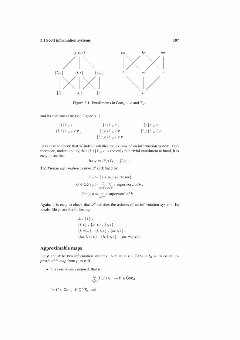
3.1 Scott information systems 107
l ε r
l,ε l,r ε,r
l,ε,r..............................................................................................................
.
.
.
.
.
.
.
.
.
.
.
.
.
.
.
.
.
.
.
.
.
.
.
.
.
.
.
.
.
.
.
.
.
.
.
.
.
.
.
.
.
.
.
.
.
.
.
.
.
.
.
.
.
.
.
.
.
.
.
.
.
.
.
.
.
.
.
.
.
.
.
.
.
.
.
.
..............................................................................................................
.
.
.
.
.
.
.
.
.
.
.
.
.
.
.
.
.
.
.
.
.
.
.
.
.
.
.
.
.
.
.
.
.
.
.
.
.
.
.
.
.
.
.
.
.
.
.
.
.
.
.
.
.
.
.
.
.
.
.
.
.
.
.
.
.
.
.
.
.
.
.
.
.
.
.
.
..............................................................................................................
..............................................................................................................
.
.
.
.
.
.
.
.
.
.
.
.
.
.
.
.
.
.
.
.
.
.
.
.
.
.
.
.
.
.
.
.
.
.
.
.
.
.
.
.
.
.
.
.
.
.
.
.
.
.
.
.
.
.
.
.
.
.
.
.
.
.
.
.
.
.
.
.
.
.
.
.
.
.
.
.
..............................................................................................................
..............................................................................................................
.
.
.
.
.
.
.
.
.
.
.
.
.
.
.
.
.
.
.
.
.
.
.
.
.
.
.
.
.
.
.
.
.
.
.
.
.
.
.
.
.
.
.
.
.
.
.
.
.
.
.
.
.
.
.
.
.
.
.
.
.
.
.
.
.
.
.
.
.
.
.
.
.
.
.
.
ε
l m r
lm lr mr
..........................................................................................................................
.
.
.
.
.
.
.
.
.
.
.
.
.
.
.
.
.
.
.
.
.
.
.
.
.
.
.
.
.
.
.
.
.
.
.
.
.
.
.
.
.
.
.
.
.
.
.
.
.
.
.
.
.
.
.
.
.
.
.
.
.
.
.
.
.
.
.
.
.
.
.
.
.
.
.
.
..........................................................................................................................
.
.
.
.
.
.
.
.
.
.
.
.
.
.
.
.
.
.
.
.
.
.
.
.
.
.
.
.
.
.
.
.
.
.
.
.
.
.
.
.
.
.
.
.
.
.
.
.
.
.
.
.
.
.
.
.
.
.
.
.
.
.
.
.
.
.
.
.
.
.
.
.
.
.
.
.
..........................................................................................................................
..........................................................................................................................
..........................................................................................................................
..........................................................................................................................
.
.
.
.
.
.
.
.
.
.
.
.
.
.
.
.
.
.
.
.
.
.
.
.
.
.
.
.
.
.
.
.
.
.
.
.
.
.
.
.
.
.
.
.
.
.
.
.
.
.
.
.
.
.
.
.
.
.
.
.
.
.
.
.
.
.
.
.
.
.
.
.
.
.
.
.
Figure 3.1: Entailments in ConC r∅ and TL .
and its entailment by (see Figure 3.1)
l ⊢C l , r ⊢C r , ε ⊢C ε ,
l,r ⊢C l,r,ε , r,ε ⊢C r,ε , l,ε ⊢C l,ε ,
l,r,ε ⊢C l,r,ε .
It is easy to check that C indeed satisfies the axioms of an information system. Fur-
thermore, understanding that l,r ⊢C ε is the only nontrivial entailment at hand, it is
easy to see that
IdeC = P f (TC )rl,r .
The Plotkin information system L is defined by
TL ≔ ε, l,m,r, lm, lr,mr ,
U ∈ ConL ≔ ∃a∈TL
∀b∈U
a superword of b ,
U ⊢L b≔ ∃a∈U
a superword of b .
Again, it is easy to check that L satisfies the axioms of an information system. Its
ideals, IdeL , are the following:
⊥ , ε ,
l,ε , m,ε , r,ε ,
l,m,ε , l,r,ε , m,r,ε ,
lm, l,m,ε , lr, l,r,ε , mr,m,r,ε .
Approximable maps
Let ρ and σ be two information systems. A relation r ⊆ Conρ ×Tσ is called an ap-
proximable map from ρ to σ if
• it is consistently defined, that is,
∀b∈V
(U,b) ∈ r→V ∈ Conσ ,
for U ∈ Conρ , V ⊆ f Tσ , and
108 3. Connections to point-free structures
• it is deductively closed, that is,
U ′ ⊢ρ U ∧ ∀b∈V
(U,b) ∈ r∧V ⊢σ b′→ (U ′,b′) ∈ r ,
for U,U ′ ∈ Conα , V ∈ Conσ and b′ ∈ Tσ .
Let us stress the fact that an approximable map need not be a single-valued mapping in
general. Write Apxρ→σ for all approximable maps from ρ to σ . One can easily gener-
alize Proposition 1.16 and show that the ideals of ρ → σ are exactly the approximable
maps from ρ to σ , that is, that Ideρ→σ = Apxρ→σ .
As already remarked in Scott’s seminal paper [51, §5] (where actually the converse
route was taken), any approximable map r from ρ to σ induces a relation r ⊆ Conρ ×Conσ by letting
(U,V ) ∈ r≔ ∀b∈V
(U,b) ∈ r .
Proposition 3.3. Let r be an approximable map from ρ to σ . For the relation r the
following hold:
1. (∅,∅) ∈ r,
2. (U,V ) ∈ r∧ (U,V ′) ∈ r→ (U,V ∪V ′) ∈ r,
3. U ′ ⊢ρ U ∧ (U,V ) ∈ r∧V ⊢σ V ′→ (U ′,V ′) ∈ r.
Conversely, if R ⊆ Conρ ×Conσ satisfies the above, then the relation R ⊆ Conρ ×Tσ
defined by
(U,b) ∈ R≔ ∃V∈Conσ
(b ∈V ∧ (U,V ) ∈ R)
is an approximable map from ρ to σ .
In what follows we will identify r with r and R with R.
Ideal-wise equality
Call two information systems ρ and σ ideal-wise equal or just equal, and write ρ ≃ σ ,
if they give rise to the same ideals up to isomorphism, that is, if Ideρ ≃ Ideσ . Ideal-
wise equal information systems define isomorphic domains (see section 3.3), hence the
overload on the isomorphism symbol “≃”. Call ρ ideal-wise smaller or just smaller
than σ , and write ρ σ , if the ideals of the former can be embedded into the ideals of
the latter, that is, if Ideρ → Ideσ . Notice that, in general, it is ρ σ ∧σ ρ 6→ ρ ≃ σ .
Let ρ = (T,Con,⊢) be an information system. Its neighborhood information sys-
tem Nρ = (NT,NCon,⊢N) is defined by
NT ≔ Con ,
U ∈ NCon≔⋃
U ∈ Con ,
U ⊢N V ≔⋃
U ⊢V .
Proposition 3.4. If ρ is an information system then Nρ is an information system, and
it is ρ ≃ Nρ .
3.1 Scott information systems 109
Proof. For reflexivity of consistency: Let U ∈ Con; then obviously U ∈ NCon by
definition. For closure under subsets: Let U ,V ∈P f (Con); then
U ∈ NCon∧V ⊆U
⇒⋃
U ∈ Con∧⋃
V ⊆⋃
U
clsr⇒⋃
V ∈ Con
⇔ V ∈ NCon .
For reflexivity of entailment: Let U ∈P f (Con) and U ∈ Con; then
U ∈U ⇒U ⊆⋃
Urefl. in ρ⇒
⋃
U ⊢U ⇔U ⊢N U .
For transitivity of entailment: Let U ,V ∈P f (Con) and W ∈ Con; then
U ⊢NV ∧V ⊢N W
⇔ ∀V∈V
U ⊢N V ∧V ⊢N W
⇔ ∀V∈V
⋃
U ⊢V ∧⋃
V ⊢W
⇔⋃
U ⊢⋃
V ∧⋃
V ⊢W
trns⇒⋃
U ⊢W
⇔U ⊢N W .
For propagation of consistency through entailment: Let U ∈P f (Con) and V ∈ Con;
then
U ∈ NCon∧U ⊢N V
⇔⋃
U ∈ Con∧⋃
U ⊢V
prpg
⇒⋃
U ∪V ∈ Con
⇔U ∪V ∈ NCon .
To show that the classes of ideals in the two information systems are isomorphic,
take the correspondence defined by the two mappings P f : Ideρ → IdeNρ and⋃
:
IdeNρ → Ideρ . It is direct to see that both of them are well-defined injections, as well
as that they are mutually inverse.
Consider now the quotient information system Qρ =(
QT,QCon,⊢Q)
, defined by
QT ≔ Con/∼ ,
[Ui]i<n ∈ QCon≔⋃
i<n
Ui ∈ Con ,
[Ui]i<n ⊢Q [V ]≔
⋃
i<n
Ui ⊢V ,
where
U ∼V ≔U ⊢V ∧V ⊢U
is the equientailment or equivalence of formal neighborhoods. An easy characteriza-
tion of equientailment in terms of closures is given by the following.
110 3. Connections to point-free structures
Proposition 3.5. It is U ∼V if and only if U =V .
Proof. The right direction follows from transitivity and the left one from reflexivity
and transitivity of entailment.
Proposition 3.6. Equientailment is compatible with QCon and ⊢Q. Furthermore, if ρis an information system then Qρ is an information system, and it is ρ ≃ Qρ .
Proof. For compatibility with QCon: Let U1, . . . ,Un ∈QCon and Ui ∼Vi, for all i =1, . . . ,n; by definition
⋃ni=1 Ui ∈ Con and Ui ⊢Vi∧Vi ⊢Ui, for all i’s; then
⋃ni=1 Ui ⊢Vi,
for all i’s, so⋃n
i=1 Vi ∈ Con, and by definition V1, . . . ,Vn ∈ QCon.
For compatibility with ⊢Q: Let U1, . . . ,Un ⊢Q U and Ui ∼ Vi, for i = 1, . . . ,n,
as well as U ∼ V ; by definition⋃n
i=1 Ui ⊢U and Ui ⊢ Vi ∧Vi ⊢Ui, for all i’s, as well
as U ⊢ V ∧V ⊢ U ; then⋃n
i=1 Vi ⊢⋃n
i=1 Ui ⊢ U ⊢ V , so by transitivity and definition
V1, . . . ,Vn ⊢Q V .
For reflexivity of consistency: Let [U ] ∈QT , that is, [U ] ∈Con/∼; from U ∈Con,
we immediately have [U ] ∈ QCon by definition. For closure under subsets: Let
[Ui]i<n,[Vj] j<m ∈P f (QT ); then
[Ui]i<n ∈ QCon∧[Vj] j<m ⊆ [Ui]i<n
⇔⋃
i<n
Ui ∈ Con∧⋃
j<m
Vj ⊆⋃
i<n
Ui
clsr⇒
⋃
j<m
Vj ∈ Con
⇔[Vj] j<m ∈ QCon .
For reflexivity of entailment: Let [Ui]i<n ∈P f (QT ) and [U ] ∈ QT ; then
[U ] ∈ [Ui]i<n ⇔ ∃i<n
[U ] = [Ui]
⇒ ∃i<n
Ui ⊢U
(⋆)⇒⋃
i<n
Ui ⊢U
⇔[Ui]i<n ⊢Q [U ] ,
where at (⋆) we used reflexivity and transitivity at ρ . For transitivity of entailment: Let
[Ui]i<n,[Vj] j<m ∈P f (QT ) and [W ] ∈ QT ; then
[Ui]i<n ⊢Q [Vj] j<m∧[Vj] j<m ⊢
Q [W ]
⇔ ∀j<m[Ui]i<n ⊢
Q [Vj]∧[Vj] j<m ⊢Q [W ]
⇔ ∀j<m
⋃
i<n
Ui ⊢Q Vj ∧
⋃
j<m
Vj ⊢Q W
(⋆)⇒⋃
i<n
Ui ⊢Q⋃
j<m
Vj ∧⋃
j<m
Vj ⊢Q W
trns⇒Uii<n ⊢W
⇔[Ui]i<n ⊢Q [W ] ,
3.2 Atomicity and coherence in information systems 111
where the step (⋆) we got by Proposition 3.1(6). For propagation of consistency through
entailment: Let [Ui]i<n ∈P f (QT ) and [V ] ∈ QT ; then
[Ui]i<n ∈ QCon∧[Ui]i<n ⊢Q [V ]
⇔⋃
i<n
Ui ∈ Con∧⋃
i<n
Ui ⊢V
prpg
⇒⋃
i<n
Ui∪V ∈ Con
⇔[Ui]i<n∪[V ] ∈ QCon .
We show that Qρ ≃ Nρ , so that Qρ ≃ ρ will follow from Proposition 3.4. For
IdeQρ → IdeNρ take u 7→ V ∈ NT | ∃U∈Con ([U ] ∈ u∧V ∈ [U ]), and for IdeNρ →IdeQρ take u 7→ [U ] ∈ QT |U ⊆ u. It is direct to see that these mappings are well-
defined injections, as well as that they are mutually inverse.
3.2 Atomicity and coherence in information systems
For an arbitrary information system ρ = (T,Con,⊢), define atomic entailment and
coherent neighborhoods respectively by
U ⊢A b≔ ∃a∈Ua ⊢ b ,
U ∈ HCon≔ ∀a,a′∈U
a,a′ ∈ Con ,
where U ∈P f (T ).
Theorem 3.7. The following hold:
1. It is ⊢A⊆⊢ and Con⊆ HCon.
2. The triples Aρ ≔ (T,Con,⊢A) and Hρ ≔ (T,HCon,⊢H) are both information
systems, where, in Hρ , entailment is extended to coherent neighborhoods U ∈HCon trivially, that is, by inductively adding all reflections and transitions of
HCon on ⊢:
U ⊢H b≔U ⊢ b∨b ∈U ∨ ∃V∈HCon
(
U ⊢H V ∧V ⊢H b)
.
3. It is clAρ(U)⊆ clρ(U) and ∀U∈Con clHρ(U) = clρ(U).
4. It is ρ Aρ and ρ Hρ .
5. Atomicity and coherence are idempotent, in the sense that A(Aρ) ≃ Aρ and
H(Hρ)≃ Hρ .
Proof. For the first statement: we have ⊢A⊆⊢ directly by definition, and reflexivity
and transitivity of ⊢, while for every U ∈ Con, by closure under subsets, we have
∀a,a′∈Ua,a′ ∈ Con, so U ∈ HCon.
For the second statement: For Aρ we have to check the laws of the definition
concerning entailment. For reflexivity, if U ∈ Con then a ⊢ a for all a ∈ U , so
112 3. Connections to point-free structures
U ⊢A a for all a ∈U . For transitivity:
U ⊢A V ∧V ⊢A cdef⇔ ∀
b∈V∃
ab∈Uab ⊢ b∧ ∃
b∈Vb ⊢ c
a≔ ab⇒ ∃a∈Ua ⊢ c
def⇔U ⊢A c
Finally, consistency propagates through atomic entailment, since it does so through
entailment in general (see previous statement).
For Hρ: Reflexivity for coherent consistency follows from the previous state-
ment, since all singletons are already in Con. For closure of coherent consistency
under subsets, let U ∈ HCon, V ⊆ U ; by closure under subsets for neighborhoods,
it is V ∈ Con, so it is a finite set; for a,a′ ∈ V , since V ⊆ U , it is a,a′ ∈ Con, so
V ∈HCon. Reflexivity of coherent entailment follows directly from the definition. For
the transitivity of coherent entailment let’s consider the most complicated case, where
U,V ∈ HConrCon with
∀b∈V
(
∃WU∈HCon
(
U ⊢H WU ∧WU ⊢H b
)
)
∧ ∃WV∈HCon
(
V ⊢H WV ∧WV ⊢H c
)
.
By applying the induction hypothesis first for WU via V to WV and then for WU via
WV to c, we get WU ⊢H c, so by definition it is U ⊢H c. For propagation of coherent
consistency through coherent entailment, let U ⊢H b for some U ∈ HCon: if U ⊢ b
then U ∪b ∈ Con ⊆ HCon; if b ∈ U , then U ∪b = U ∈ HCon; if U ⊢H V and
V ⊢H b for some V ∈HCon, then, by the induction hypothesis, it is U ∪V ∈HCon and
U ∪V ⊢H b; by the induction hypothesis again, U ∪V ∪b ∈HCon; by closure under
subsets, U ∪b ∈ HCon.
The third statement is direct to show.
For the fourth statement: We show that Ideρ ⊆ IdeAρ ; let u ∈ Ideρ ; if U ⊆ f u, then
U ∈ Con by the consistency in ρ; if further U ⊢A b, then U ⊢ b since ⊢A⊆⊢, so b ∈ u
by deductive closure in ρ .
We now show that Ideρ ⊆ IdeHρ : let u ∈ Ideρ ; if U ⊆ f u, then U ∈ Con ⊆ HCon
by the consistency in ρ; if further U ⊢A b, then U ⊢ b since U ∈ Con again, so b ∈ u by
deductive closure in ρ .
For the fifth statement: For the idempotence of A, the only thing we have to show
is that ⊢AA=⊢A:
U ⊢AA
b⇔ ∃a∈Ua ⊢A b
⇔ ∃a∈U
∃a′∈a
a′ ⊢ b
⇔ ∃a∈Ua ⊢ b .
So it is A(Aρ)≃ Aρ , actually with the trivial isomorphism. For the idempotence of H,
we have ConHρ = HConρ , so:
U ∈ H(HConρ)⇔ ∀a,a′∈U
a,a′ ∈ HConρ
(∗)⇔ ∀
a,a′∈Ua,a′ ∈ Conρ
⇔U ∈ HConρ ,
3.3 Coherent point-free structures 113
and U ∈ ConHρ ; step (∗) holds since two-element sets that are consistent are also
coherently consistent and vice versa. Finally, let U ⊢HHb; if it is U ⊢H b or b ∈U ,
then we’re done; if there is a V ∈ H(HCon) such that U ⊢HHV and V ⊢HH
b, then, as
we just saw, it is V ∈ HCon, which means that U ⊢H V and V ⊢H b, so by transitivity,
U ⊢H b.
Notice that we cannot do better than Theorem 3.7(4) in general. Indeed, both atom-
icity and coherence may provide “extra” ideals that are absent in the original informa-
tion system. For example, consider the information systems C and L (page 106); it is
direct to check that
IdeC = l,r ∈ IdeAC
(follows by the Coquand counterexample) and also that
IdeL = l,m,r,ε ∈ IdeHL .
So atomic and coherent information systems are generally ideal-wise richer. Notice,
moreover, that they are the richest we can get in this manner, a fact that is expressed by
Theorem 3.7(5).
3.3 Coherent point-free structures
Formal topology is point-free topology from a predicative and constructive viewpoint
([40], [39], [42], [9]). Links between domain theory and formal topology have been
noticed and studied by several people already (see [41], [38], [30], [33], [52]). The
main objective of this section is to match coherent information systems to respective
“coherent” point-free structures, domains included.
The basic problem that one faces in such an endeavor lies, not surprisingly, in the
very nature of coherence. By its definition (page 111), coherence involves comparisons
between tokens, but tokens are unobservable in any point-free setting; everything there
starts with neighborhoods. Luckily, we have the following easy characterization.
Proposition 3.8. A finite set of tokens is a coherent neighborhood if and only if every
two of its subsets have a coherent union: it is U ∈HCon if and only if U ∈P f (T ) and
U1∪U2 ∈ HCon, for any U1,U2 ⊆U.
Notice that we could equivalently say “U0 ∈ HCon for any U0 ⊆U” instead of “U1 ∪U2 ∈HCon for any U1,U2 ⊆U”; we choose the latter to stress that the issue of validity
of a neighborhood in a coherent system is raised from comparisons of its tokens, to
comparisons of its subsets. The coherence conditions (3.1), (3.2), and (3.4), that we
pose in the following are all modeled after Proposition 3.8.
In this section we restrict ourselves to the case where we have countable carrier
sets.
Domains
We start with the known correspondence of arbitrary Scott information systems and
domains (of countable base), which we quickly recount here without proofs, to set the
mood for what comes next (see Appendix A for relevant basic notions and facts that
we may refer to but omit here).
114 3. Connections to point-free structures
Let D = (D,⊑,⊥, lub) be a domain and define I(D)≔ (T,Con,⊢) by
T ≔ Dc ,
uii∈I ∈ Con≔ uii∈I ⊆f Dc∧ lubuii∈I ∈ D ,
uii∈I ⊢ u≔ u⊑ lubuii∈I .
Notice that, by Fact A.8.1, if uii∈I ∈ Con then lubuii∈I ∈ Dc. Conversely, for an
information system ρ = (T,Con,⊢), define D(ρ)≔ (Ideρ ,⊆,⊥,⋃).
The following comprises Propositions 6.1.6, 6.1.8, and Theorem 6.1.91 of [52].
Proposition 3.9. If D is a domain and ρ an information system, then I(D) is an in-
formation system and D(ρ) a domain, where compact elements are given by deductive
closures, that is, where D(ρ)c = Conρ .
Furthermore, if D is a domain then IdeI(D) ≃ D, through the isomorphism pair
u 7→ lubu and u 7→ apx(u), where apx(u) is the set of the compact approximations of u.
Let now r be an approximable map from ρ to σ . Define a mapping D(r) : D(ρ)→D(σ) by
D(r)(u)≔⋃
V ∈ Conσ |U ⊆ f u∧ (U,V ) ∈ r .
Conversely, let f be a continuous mapping from a domain D to a domain E. Define a
relation I( f )⊆ ConI(D)×ConI(E) by
(U,V ) ∈ I( f )≔ lubV ≤ f (lubU) .
These establish a bijective correspondence, as the following statement expresses (The-
orem 6.1.12 of [52]).
Proposition 3.10. If r is an approximable map from ρ to σ then D(r) : D(ρ)→ D(σ)is a continuous mapping. Conversely, if f : D→ E is a continuous mapping then I( f )is an approximable map from I(D) to I(E). Furthermore, the collection of continuous
mappings from D to E is in a bijective correspondence with the collection of approx-
imable maps between I(D) and I(E).
Coherent domains
Let D = (D,⊑,⊥) be a domain and uii∈I ⊆f Dc an arbitrary finite set of compact
elements. Call D a coherent domain if
lubuii∈I ∈ Dc ↔ ∀i, j∈I
lubui,u j ∈ Dc . (3.1)
Note that the choice of Dc instead of the more modest D is justified by Fact A.8(1).
Theorem 3.11. Let D be a coherent domain and ρ a coherent information system.
Then I(D) is a coherent information system and D(ρ) is a coherent domain.
Proof. Let D be a coherent domain and uii∈I ∈ ConI(D). By the definition of I(D),
uii∈I ⊆f Dc and lubuii∈I ∈ D. By Fact A.8(1), lubuii∈I ∈ Dc. By the coherence,
∀i, j∈I lubui,u j ∈ Dc and we’re done.
1This is called second representation theorem in [52], besides the first representation theorem (“a domain
is represented by its compact elements”, see Fact A.9) and the third representation theorem (“a domain is
represented by its induced Scott space”).
3.3 Coherent point-free structures 115
Let now ρ be a coherent information system and Uii∈I ⊆f Conρ . By the coher-
ence and Proposition 3.8, it is
⋃
i∈I
Ui ∈ Conρ ↔ ∀i, j∈I
Ui∪U j ∈ Conρ ,
so also⋃
i∈I
Ui ∈ Conρ ↔ ∀i, j∈I
Ui∪U j ∈ Conρ .
Precusl’s
A preordered conditional upper semilattice with a distinguished least element, or just
precusl, is a ‘consistently complete preordered set with a distinguished least element’,
that is, a quadruple P = (N,⊑,⊔,⊥) where⊑ is a preorder on N,⊥ is a (distinguished)
least element and ⊔ is a partial binary operation on N which is defined only on con-
sistent pairs, that is, on pairs having an upper bound, and then yields a (distinguished)
least upper bound:
U ⊔V ∈ N ≔ ∃W∈N
(U ⊑W ∧V ⊑W ) ,
U ⊔V ∈ N ⇒U ⊑U ⊔V ∧V ⊑U ⊔V
∧ ∀W∈N
(U ⊑W ∧V ⊑W →U ⊔V ⊑W ) .
We think of N as “a set of formal basic opens”, ⊑ as “formal inclusion”, ⊥ as “a
formal empty set” and ⊔ as “a formal union”. Call a subset u⊆ N a precusl ideal when
it satisfies
⊥ ∈ u ∧ ∀U,V∈u
U ⊔V ∈ u ∧ ∀U∈u
(V ⊑U →V ∈ u) .
Write IdeP for the class of all precusl ideas of P. Observe that the second of the three
requirements for a precusl ideal expresses the property of being upward directed, so
it follows that any finite subset in a precusl ideal will have a least upper bound in the
ideal (for details on the relation of precusl’s and information systems that are not given
here, one should consult [52, § 6.3]).
Let now P = (N,⊑,⊔,⊥) be a precusl and define I(P) = (T,Con,⊢) by
T ≔ N ,
U ∈ Con≔U ⊆ f N∧⊔
U ∈ N ,
U ⊢U ≔U ⊑⊔
U .
Conversely, let ρ = (T,Con,⊢) be an information system and define P(ρ) =(N,⊑,⊥,⊔) by
N ≔ Con ,
U ⊑V ≔V ⊢U ,
⊥≔ ∅ ,
U ⊔V ≔U ∪V if U ∪V ∈ Con .
The following is Theorem 6.3.4 of [52].
116 3. Connections to point-free structures
Proposition 3.12. If P is a precusl and ρ an information system, then I(P) is an
information system and P(ρ) is a precusl. Furthermore, it is IdeP = IdeI(P) and
Ideρ ≃ IdeP(ρ).
Proof. We just show the existence of isomorphisms between corresponding informa-
tion system ideals and precusl ideals, as the proof is omitted in the above reference.
For IdeP ⊆ IdeI(P), let u∈ IdeP and U ⊆ f u. Since u is an ideal in P,⊔
U ∈ u⊆N,
so U ∈ ConI(P) by definition. If further U ⊢I(P) U , it is U ⊑⊔
U by definition, so
U ∈ u, again because u is an ideal in P.
For IdeI(P)⊆ IdeP, let u∈ IdeI(P). That⊥≔∅∈ u, follows from downward closure
in I(P). Let U,V ∈ u; since u is an ideal in I(P), it is U,V∈ConI(P), and then U⊔V ∈N by definition; since U,V ⊢I(P) U ⊔V and u is an ideal in I(P), it is U ⊔V ∈ u. If
now U ∈ u and V ⊑U , then U ⊢I(P) V by definition, and V ∈ u follows again because
u is an ideal in I(P).For Ideρ ≃ IdeP(ρ) take the following isomorphism pair:
Ideρ ∋ u 7→P f (u) ∈ IdeP(ρ) ,
IdeP(ρ) ∋ u 7→⋃
u ∈ Ideρ .
These mappings are well-defined. For the right embedding, it is obviously ⊥ ≔ ∅ ∈P f (u); for every U,V ∈ P f (u) it is also U ∪V ⊆ f u, so it is U ⊔V ∈ P f (u) by
definition; if U ∈P f (u) and V ⊑U , then⋃U=U ⊢V by definition, so since u is an
ideal in ρ , it is V ⊆ f u, that is, V ∈P f (u). For the left embedding, if aii<n ⊆f⋃
u,
then ∀i<n∃Ui∈u ai ∈Ui; since u is an ideal in P(ρ), it is⊔
i<n Ui ∈ u ⊆ f NP(ρ), so, by
definition,⋃
i<n Ui ∈ Con; by closure of consistency under subsets in ρ , it is aii<n ∈Con. If now U ⊆ f
⋃u and U ⊢ a, then a ⊑U by definition; since u is an ideal in
P(ρ), we have a ∈ u, so a ∈⋃
u.
It remains to show that the two embeddings are indeed mutually inverse. Let u ∈Ideρ ; we have
a ∈⋃
P f (u)⇔ ∃U⊆ f u
a ∈U(⋆)⇔ a ∈ u ,
where (⋆) holds leftwards for U ≔ a, and
aii<n ∈P f
(⋃
u)
⇔aii<n ⊆f⋃
u
⇔ ∀i<n∃
Ui∈uai ∈Ui
(⋆)⇔ ∀
i<n∃
Ui∈uai ⊑Ui
(⋆)⇔ ∀
i<n∃
Ui∈uai ⊑
⊔
i<n
Ui
(⋆)⇔aii<n ∈ u ,
where (⋆) hold leftwards for Ui ≔ ai, i < n.
A precusl approximable map from P to P′ is a relation R ⊆ N×N′ which satisfies
the following:
• (⊥,⊥′) ∈R,
• (U,V ) ∈R ∧ (U,V ′) ∈R → (U,V ⊔V ′) ∈R,
3.3 Coherent point-free structures 117
• U ⊑U ′∧ (U,V ) ∈R ∧V ′ ⊑V → (U ′,V ′) ∈R,
where (U,V ⊔V ′) ∈R naturally implies that V ⊔V ′ is defined. Write ApxP→P′ for all
precusl approximable maps from P to P′. For every R ∈ ApxP→P′ define a relation
I(R)⊆ ConI(P)×ConI(P′) by
(U ,V ) ∈ I(R)≔(⊔
U ,⊔
V
)
∈R .
Conversely, let r be an approximable map from ρ to σ . Define a relation P(r) ⊆NP(ρ)×NP(σ) by
(U,V ) ∈ P(r)≔ (U,V ) ∈ r .
One can show (see [52, pp. 151–2]) that these establish a bijective correspondence.
Proposition 3.13. If r is an approximable map from ρ to σ then P(r) is a precusl
approximable map from P(ρ) to P(σ). Conversely, if R is a precusl approximable
map from P to P′ then I(R) is an approximable map from I(P) to I(P′). Furthermore,
it is Apxρ→σ ≃ ApxP(ρ)→P(σ) and ApxP→P′ ≃ ApxI(P)→I(P′).
Coherent precusl’s
Call a precusl coherent if it satisfies the following property for a finite collection U ⊆ f
N:⊔
U ∈ N ↔ ∀U,V∈U
U ⊔V ∈ N . (3.2)
Theorem 3.14. If P is a coherent precusl then I(P) is a coherent information system.
Conversely, if ρ is a coherent information system then P(ρ) is a coherent precusl.
Proof. Suppose first that P is coherent, that is, such that (3.2) holds for all U ⊆ f N.
Let U ∈ ConI(P); by the definition,
U ⊆ f N∧⊔
U ∈ N(3.2)⇔U ⊆ f N∧ ∀
U,V∈U
U ⊔V ∈ N
def⇔U ⊆ f N∧ ∀
U,V∈U
U,V ∈ ConI(P) ,
so I(P) is a coherent information system.
Now suppose that ρ is a coherent information system, that is, such that
U ∈ Con↔ ∀a,b∈U
a,b ∈ Con , (3.3)
for all U ⊆ f T . Let U ⊆ f NP(ρ), that is, U ⊆ f Con; we have
⊔
U ∈ NP(ρ)def⇔⋃
U ∈ Con
(⋆)⇔⋃
U ⊆ f T ∧ ∀U,V⊆
⋃U
U ∪V ∈ Con
def⇔⋃
U ⊆ f T ∧ ∀U,V⊆
⋃U
U ⊔V ∈ NP(ρ)
⇒ ∀U,V∈U
U ⊔V ∈ NP(ρ) ,
118 3. Connections to point-free structures
where at (⋆) we used (3.3) and Proposition 3.8. Conversely, we have
U ⊆ f NP(ρ)∧ ∀U,V∈U
U ⊔V ∈ NP(ρ)def⇔U ⊆ f Con∧ ∀
U,V∈U
U ⊔V ∈ Con
(3.3)⇔U ⊆ f Con∧ ∀
U,V∈U∀
a,b∈U∪Va,b ∈ Con
⇒U ⊆ f Con∧ ∀a,b∈
⋃U
a,b ∈ Con
(3.3)⇔⋃
U ∈ Con
def⇔⊔
U ∈ NP(ρ) ,
so P(ρ) is indeed a coherent precusl.
Scott–Ershov formal topologies
The structure of a “formal topology” was defined by Giovanni Sambin as early as
1987 in [37], and as the area has developed a number of alternative definitions has
appeared. Suitable for our purposes is a version of the definition in [30], whose main
difference from Sambin’s original is the disposal of the “positivity predicate”—see [30,
§2.4 ] or [39, Footnote 13] for a justification of this. In fact, we depart a bit from this
definition as well, in that we require the presence of a top element among the formal
basic opens, this is however an inessential difference (see Exercise 6.5.21 of [52]). For
a list of nomenclature discrepancies between our exposition and the literature, see notes
in 3.4.
We will use order-theoretic notions which are dual to notions appearing before,
namely a greatest or top element and greatest lower bounds of sets of elements; all
these are to be understood in the usual order-theoretic way.
Define a formal topology as a triple T = (N,⊑,≺) where N is the collection of
formal basic opens, ⊑ ⊆ N ×N is a preorder with a top element ⊤, which formal-
izes inclusion between basic opens, and ≺ ⊆ N×P(N), called covering, formalizes
inclusion between arbitrary opens, and satisfies the following:
1. it is reflexive,
U ∈U →U ≺U ,
2. it is transitive,
U ≺U ∧U ≺ V →U ≺ V ,
3. it is localizing,
U ≺U ∧U ≺ V →U ≺U ↓ V ,
and
4. it extends formal inclusion between formal basic opens,
V ⊑U ∧U ≺U →V ≺U ,
where U ≺ V ≔ ∀U∈U U ≺ V and
U ↓ V ≔ W ∈ N | ∃U∈U
∃V∈V
(W ⊑U ∧W ⊑V ) .
A formal point in T is a subset u⊆ N such that
3.3 Coherent point-free structures 119
1. ⊤ ∈ u,
2. ∀U,V∈u∃W∈u (W ⊑U ∧W ⊑V ),
3. ∀U∈u (U ≺U → ∃V∈U V ∈ u).
Dually to the case of precusl ideals, the second of the three requirements for a formal
point expresses the preperty of being downward directed, so it follows that any finite
subset in a formal point will have a greatest lower bound in the ideal. Denote the
collection of formal points of T by PtT .
Call a formal topology T unary if
U ≺U → ∃V∈U
U ≺V ,
where we write U ≺V for U ≺ V, and consistently complete if
∀U,V∈N
(
∃W∈N
(W ⊑U ∧W ⊑V )→ ∃W∈N
W =U ⊓V
)
,
where
U denotes the greatest lower bound of U . Finally, call T a Scott–Ershov
formal topology if it is both unary and consistently complete.
One can prove that every domain can be represented by the collection of formal
points of a certain Scott–Ershov formal topology (see Theorem 4.35 of [30] and Theo-
rem 6.2.15 of [52]). Here we proceed to link formal topologies directly to information
systems.
Let T = (N,⊑,≺) be a Scott–Ershov formal topology. Define I(T ) = (T,Con,⊢)by
T ≔ N ,
U ∈ Con≔U ⊆ f N∧
U ∈ N ,
U ⊢U ≔
U ⊑U .
Conversely, let ρ =(T,Con,⊢) be an information system. Define F(ρ)= (N,⊑,≺)by
N ≔ Con ,
U ⊑V ≔U ⊢V ,
U ≺U ≔ ∃V∈U
U ⊢V .
Note that the definition is independent from the choice of representatives—see Propo-
sition 3.5.
Proposition 3.15. If T is a Scott–Ershov formal topology and ρ an information sys-
tem, then I(T ) is an information system and F(ρ) is a Scott–Ershov formal topology.
Furthermore, it is PtT = IdeI(T ) and Ideρ ≃ PtF(ρ).
Proof. First let T be a Scott–Ershov formal topology. We check the defining prop-
erties of an information system for I(T ). For reflexivity of consistency, let U ∈ N; it
is U ⊑U , so
U ∈ N and U ∈ Con by definition. For closure under subsets, let
U ∈ Con and V ⊆U ; then
U ∈ N and ∀V∈V
U ⊑V , so
V ∈ N and V ∈ Con
120 3. Connections to point-free structures
by definition. For reflexivity of entailment, let U ∈ Con and U ∈U ; then
U ⊑U ,
so U ⊢U by definition. For transitivity of entailment, let U ⊢ V and V ⊢W ; then
U ⊑
V and
V ⊑W ; by transitivity we get
U ⊑W , so U ⊢W by definition.
Finally, for propagation of consistency through entailment, let U ∈ Con and U ⊢ V ;
by definition,
U ∈ N and
U ⊑ V , so
(U ∪V) ∈ N and U ∪V ∈ Con by
definition.
Now let ρ be an information system. We check the defining properties of a Scott–
Ershov formal topology for F(ρ). That ⊑ is a preorder with ⊤ ≔ ∅ is direct to see.
For reflexivity of covering, let U ∈ U ; since U ⊢U , it is U ≺ U by definition. For
transitivity of covering, we have
W ≺U ∧U ≺ V ⇔ ∃U∈U
(
W ⊢U ∧ ∃V∈V
U ⊢V
)
trns⇒ ∃
V∈V
W ⊢V
⇔W ≺ V .
For localization, we have
W ≺U ∧W ≺ V ⇔ ∃U∈U
(
W ⊢U ∧ ∃V∈V
W ⊢V
)
⇔ ∃U∈U
(
W ⊑U ∧ ∃V∈V
W ⊑V
)
⇔W ∈U ↓ V
refl⇒W ≺U ↓ V .
To show that the covering extends formal inclusion between formal basic opens, we
have:
W ⊑U ∧U ≺ V ⇔W ⊢U ∧ ∃V∈V
U ⊢V
trns⇒ ∃
V∈V
W ⊢V
⇔W ≺ V .
So F(ρ) is indeed a formal topology. To show that it is unary is easy: let U ≺U ; by
definition there is a V ∈U , for which U ⊢V , that is, U ⊑V ; by reflexivity and exten-
sion, we get U ≺V. To show, finally, that it is consistently complete, let U ,V ,W ∈N,
with W ⊑ U and W ⊑ U , that is, W ⊢ U and W ⊢ V ; by Proposition 3.1(6), we get
W ⊢U ∪V , and so, W ⊑U ∪V ; let U ⊓V ≔U ∪V ; that this does the job is direct to
see.
We now show the bijective correspondence between information system ideals and
formal points. For PtT ⊆ IdeI(T ), let u ∈ PtT and U ⊆ f u. Since u is downward
directed in T , it is
U ∈, and so U ∈ ConI(T ) by definition. If further U ⊢I(T ) U ,
it is
U ⊑U by definition, and
U ≺ U; hence U ∈ u by the third formal point
property.
For IdeI(T ) ⊆ PtT , let u ∈ IdeI(T ). That ⊤ = ∅ ∈ u, follows from downward
closure in I(T ). Let U,V ∈ u; by the consistency in I(T ), U,V ∈ConI(T ), and then
U ⊓V ∈ N by definition; since U,V ⊢I(T ) U ⊓V , it is U ⊓V ∈ u by the deductive
3.3 Coherent point-free structures 121
closure in I(T ). If now U ∈ u and U ≺U , then, since T is unary, we have ∃V∈U U ⊑V , and ∃V∈U U ⊢I(T ) V by the definition, so that ∃V∈U V ∈ u follows from the
deductive closure in I(P).
For Ideρ ≃ PtF(ρ) take the following isomorphism pair:
Ideρ ∋ u 7→Pc(u) ∈ PtF(ρ)
PtF(ρ) ∋ u 7→⋃
u ∈ Ideρ
where Pc(u)≔ UU⊆ f u contains the closures of subsets of u.
Indeed, for the right embedding, since∅⊆ f u, it is⊤∈Pc(u); for every U,V ⊆ f u,
since U ∪V ⊆ f u, it is also U ⊓V ∈Pc(u); if U ⊆ f u and U ≺U , then ∃V∈UU ⊑V ,
that is, ∃V∈UU ⊢V by definition; then ∃V∈U
V ⊆ f u by deductive closure in ρ .
For the left embedding, if aii<n ⊆f⋃
u, then ∀i<n∃Ui∈u Ui ⊢ ai; since u is down-
ward directed in F(ρ) we have that ∃W∈u∀i<n W ⊑Ui; by definition, ∃W∈u∀i<n W ⊢Ui ⊢ ai, so aii<n ∈ Con by transitivity of entailment and Proposition 3.1(6). If now
U ⊆ f⋃
u and U ⊢ a, then, by definition, U ⊑ a, that is U ≺ a; by the third formal
point property in F(ρ), we have a ∈ u, so a ∈⋃
u.
That the two embeddings are mutually inverse is also quite direct. Indeed, let u ∈Ideρ . We have
a ∈⋃
Pc(u)⇔ ∃U⊆ f u
U ⊢ a(⋆)⇔ a ∈ u
where (⋆) holds leftwards for U ≔ a, and
aii<n ∈Pc
(⋃
u)
⇔aii<n ⊆f⋃
u
⇔ ∀i<n∃
Ui∈u
Ui ⊢ ai
(⋆)⇔ ∀
i<n∃
Ui∈u
Ui ⊑ ai
(⋆)⇔ ∀
i<n∃
Ui∈u
i<n
Ui ⊑ ai
(⋆)⇔ ∀
i<n∃
Ui∈u
i<n
Ui ≺ ai
(⋆)⇔ ∀
i<nai ∈ u
⇔aii<n ∈ u
⇔aii<n ∈ u
where (⋆) hold leftwards for Ui ≔ ai, i < n.
An approximable map of Scott–Ershov formal topologies from T to T ′ is a rela-
tion R ⊆ N×N′ which satisfies the following:
• (⊤,⊤′) ∈R,
• (U,V ) ∈R ∧ (U,V ′) ∈R → (U,V ⊓V ′) ∈R,
• U ′ ⊑U ∧ (U,V ) ∈R ∧V ⊑V ′→ (U ′,V ′) ∈R.
122 3. Connections to point-free structures
Write ApxT →T ′ for all approximable maps of Scott–Ershov formal topologies from
T to T ′. For every R ∈ ApxT →T ′ define a relation I(R)⊆ ConI(T )×ConI(T ′) by
(U ,V ) ∈ I(R)≔(
U ,
V
)
∈R .
Conversely, let r be an approximable map from ρ to σ . Define a relation F(r) ⊆NF(ρ)×NF(σ) by
(U ,V ) ∈ F(r)≔ (U,V ) ∈ r .
Again, it is easy to see that the definition does not rely on the choice of the representa-
tives, due to deductive closure of r.
We show that these establish a bijective correspondence.
Proposition 3.16. If r is an approximable map from ρ to σ then F(r) is an approx-
imable map of Scott–Ershov formal topologies from F(ρ) to F(σ). Conversely, if R is
an approximable map of Scott–Ershov formal topologies from T to T ′ then I(R) is an
approximable map from I(T ) to I(T ′). Furthermore, it is Apxρ→σ ≃ ApxF(ρ)→F(σ)
and ApxT →T ′ ≃ ApxI(T )→I(T ′).
Proof. Let r be an approximable map from ρ to σ . Since, by Proposition 3.3, (∅,∅) ∈r, it is (⊤,⊤′) ∈ F(r). If (U ,V ),(U ,V ′) ∈ F(r), then, by definitions, (U,V ∪V ′) ∈ r,
so (U ,V ∪V ′) ∈ F(r), and (U ,V ⊓V ′) ∈ F(r). If U ′ ⊑U , (U ,V ) ∈ F(r) and V ⊑ V ′,
then, by definitions, U ′ ⊢U , (U,V ) ∈ r and V ⊢ V ′ respectively, so, (U ′,V ′) ∈ r and
(U ′,V ′) ∈ F(r).
Conversely, let R be an approximable map of Scott–Ershov formal topologies from
T to T ′. Since (⊤,⊤′) ∈R, it is (∅,∅) ∈ I(R). If (U ,V ),(U ,V ′) ∈ I(R), then, by
definition, (
U ,
V ) ,(
U ,
V ′) ∈R; since R is an approximable map of Scott–
Ershov formal topologies, (
U ,(
V )⊓ (
V ′)) ∈R, or, (
U ,
(V ⊓V ′)) ∈R,
that is, (U ,V ⊓V ′) ∈ I(R). If now U ′ ⊢U , (U ,V ) ∈ I(R) and V ⊢ V ′, by defini-
tion we obtain
U ′⊑
U , (
U ,
V )∈R and
V ⊑
V ′; then (
U ′,
V ′)∈R, so (U ′,V ′) ∈ I(R).
We show that F : Apxρ→σ → ApxF(ρ)→F(σ) is bijective. To show injectivity, let
F(r) = F(r′); then
(U,V ) ∈ rdef.F⇔ (U ,V ) ∈ F(r)⇔ (U ,V ) ∈ F(r′)
def.F⇔ (U,V ) ∈ r′ ,
so r = r′. To show surjectivity, let R ∈ ApxF(ρ)→F(σ); set
(U,V ) ∈ r≔ (U ,V ) ∈R ;
it is straightforward to check that r ∈ Apxρ→σ and F(r) = R.
We show finally that I : ApxT →T ′ → ApxI(T )→I(T ′) is bijective. To show in-
jectivity, let I(R) = I(R ′) and (U,V ) ∈ R; then, by the definition of I, there are
U ∈ ConI(T ) and V ∈ ConI(T ′), such that U =
U , V =
V and (U ,V ) ∈ I(R);by the assumption we get equivalently that (U ,V ) ∈ I(R), so (U,V ) ∈ R, and
R = R ′. To show surjectivity, let r ∈ ApxI(T )→I(T ′); set
(U,V ) ∈R ≔ ∃U ∈ConI(T )
∃V ∈ConI(T ′)
(
U =
U ∧V =
V ∧ (U ,V ) ∈ r)
;
3.3 Coherent point-free structures 123
it is R ∈ ApxT →T ′ , since (i) by r ∈ ApxI(T )→I(T ′) we get (∅,∅) ∈ r, which yields
(⊤,⊤′) ∈R, (ii) it is
(U,V1) ∈R ∧ (U,V2) ∈R
⇔ ∃U1,V1
(
U =
U1∧V1 =
V1∧ (U1,V1) ∈ r)
∧ ∃U2,V2
(
U =
U2∧V2 =
V2∧ (U2,V2) ∈ r)
(∗)⇒ ∃
U ,V1,V2
(
U =
U ∧V1 =
V1∧V2 =
V2
∧ (U ,V1) ∈ r∧ (U ,V2) ∈ r)
⇒ ∃U ,V1,V2
(
U =
U ∧V1 =
V1∧V2 =
V2∧ (U ,V1∪V2) ∈ r)
(∗∗)⇒ ∃
U ,V
(
U =
U ∧V1⊓V2 =
V ∧ (U ,V ) ∈ r)
⇔ (U,V1⊓V2) ∈R ,
where (∗) holds for U ≔ U, and (∗∗) for V ≔ V1∪V2, and (iii) it is
U ′ ⊑U ∧ (U,V ) ∈R ∧V ⊑V ′
⇔U ′ ⊑U ∧ ∃U ,V
(
U =
U ∧V =
V ∧ (U ,V ) ∈ r)
∧V ⊑V ′
(∗)⇒ ∃
U ′
(
U ′ =
U′∧ ∀
U∈U
U′ ⊢I(T ) U
)
∧ ∃U ,V
(
U =
U ∧V =
V ∧ (U ,V ) ∈ r)
∧V ⊢I(T ′) V ′
(∗∗)⇒ ∃
U ′,V ′
(
U ′ =
U′∧V ′ =
V′∧ (U ′,V ′) ∈ r
)
⇔ (U ′,V ′) ∈R ,
where (∗) holds for U ′≔ U and because
V ⊑V ′⇒
V ⊑V ′⇒ V ⊢I(T ′) V ′ ,
and (∗∗) holds for V ′≔ V and because r is an approximable map; finally, direct
application of the definitions gives
(U ,V ) ∈ I(R)⇔(
U ,
V
)
∈R ⇔ (U ,V ) ∈ r ,
which means that I(R) = r.
Coherent Scott–Ershov formal topologies
Call a Scott–Ershov formal topology coherent if it satisfies the following property for
a finite collection U ⊆ f N:
U ∈ N ↔ ∀U,V∈U
U ⊓V ∈ N . (3.4)
124 3. Connections to point-free structures
Theorem 3.17. If T is a coherent Scott–Ershov formal topology then I(T ) is a co-
herent information system. Conversely, if ρ is a coherent information system then F(ρ)is a coherent Scott–Ershov formal topology.
Proof. Suppose first that T is coherent, that is, such that (3.4) holds for all U ⊆ f N.
Let U ∈ ConI(T ); by definition,
U ⊆ f N∧
U ∈ N(3.4)⇔U ⊆ f N∧ ∀
U,V∈U
U ⊓V ∈ N
def⇔U ⊆ f N∧ ∀
U,V∈U
U,V ∈ ConI(T ) ,
so I(T ) is a coherent information system.
Now suppose that ρ is a coherent information system, that is, such that
U ∈ Con↔ ∀a,b∈U
a,b ∈ Con , (3.3)
for all U ⊆ f T . Let U ⊆ f NF(ρ), that is, U ⊆ f Con; we have
U ∈ NF(ρ)def⇔⋃
U ∈ Con
(⋆)⇔ ∀
U,V⊆ f⋃
U
U ∪V ∈ Con
def⇔ ∀
U,V⊆ f⋃
U
U ⊓V ∈ NF(ρ)
⇒ ∀U ,V∈U
U ⊓V ∈ NF(ρ) ,
where at (⋆) we used (3.3) and Proposition 3.8. Conversely, we have
U ⊆ f NF(ρ)∧ ∀U ,V∈U
U ⊓V ∈ NF(ρ)def⇔U ⊆ f Con∧ ∀
U ,V∈U
U ⊓V ∈ Con
(3.3)⇔U ⊆ f Con∧ ∀
U ,V∈U
∀a,b∈U∪V
a,b ∈ Con
⇒U ⊆ f Con∧ ∀a,b∈
⋃U
a,b ∈ Con
(3.3)⇔⋃
U ∈ Con
def⇔
U ∈ NF(ρ) ,
so F(ρ) is indeed a coherent Scott–Ershov formal topology.
3.4 Notes
On the notion of atomicity
The defining property of a unary formal topology (page 119) looks similar to the atom-
icity property for an information system (page 111)—in fact, unary formal topologies
are called “atomic” by Erik Palmgren in a preliminary version of [33]—but the two are
not essentially related from our viewpoint.
The property of being unary for a formal topology expresses atomicity of compact
covering, whereas in information systems we have atomicity of information flow: in the
3.4 Notes 125
first case, an “atom” would be a formal basic open while in the second case, an atom
(that is, a token) represents a simple piece of data.
In order to avoid confusions, one should notice how the transition from an infor-
mation system to a point-free structure—domains included—involves jumping from
the level of atomic pieces of data to (finitely determined) sets of atomic pieces of data:
atomicity of information appears in the presence of atomic pieces of data, which be-
come indiscernible when one moves to a point-free setting (see however the last note).
On the notion of coherence
Coherence in domain theory is in no way considered here for the first time. Coherent
cpo’s appear already in Gordon Plotkin’s [36], where he attributes the notion to George
Markowsky and Barry Rosen [29]. In the handbook chapter of Samson Abramsky and
Achim Jung [1], coherence is studied in the more general setting of continuous do-
mains. Viggo Stoltenberg-Hansen et al [52] introduce the notion too in an exercise. We
should also mention Jean-Yves Girard’s coherence spaces [14], which he uses alter-
natively to Scott–Ershov domains. On the other hand, coherence has been considered
in point-free topology as well, at least since Peter Johnstone’s [20], where coherent
locales are discussed.
Featuring Coquand and Plotkin
Both of the finite Scott information systems C and L of section 3.1 are elaborations
of existing counterexamples.
The first one, due to Thierry Coquand, was first given as a counterexample to atom-
icity in algebraic information systems (see page 47). In Chapter 2 however, we have
shown that atomicity remains a concept worth exploring, since it lies in the very fun-
daments of the more general algebraic entailment, and at the same time gives rise to
surprising and utilizable notions, namely, matrices on the base-type case, and eigen-
neighborhoods in the higher-type case. And of course, it is a perfectly sufficient prop-
erty for algebras like natural numbers N or boolean numbers B, which have at most
unary constructors (see Chapter 1).
The second Scott information system stems from Plotkin’s [36], where he uses the
entailment graph of L as an example of a “consistently complete” but not “coher-
ent” complete partial order. It is indeed Plotkin’s counterexample to coherence: in the
entailment diagramme of L in Figure 3.1, one has l,m,l,r,m,r ∈ ConL but
l,m,r < ConL .
Notice also that C is non-atomic but coherent, and that L is incoherent but atomic.
Dues and nomenclature discrepancies
The questions answered in sections 3.2 and 3.3 occurred to the author at the 3WFTop
workshop; the results were presented for the first time in a Forschungstutorium held at
LMU during the winter semester of 2007–8 and led by Peter Schuster.
Giovanni Sambin et al [41] call consistently complete ordered sets coherent. Sara
Negri [30] says Scott formal topology for a unary formal topology and consistently
complete Scott formal topology for a Scott–Ershov formal topology (modulo the pres-
ence of a top formal basic open). Viggo Stoltenberg-Hansen et al [52] say formal space
for a consistently complete formal topology and Scott space for a Scott–Ershov formal
topology.
126 3. Connections to point-free structures
Outlook
The issue of linking the theory of information systems and formal topology has many
facets, at least as many as the various point-free structures that are currently studied by
the community. Apart from the ones that we have covered in this chapter, further links
should be attainable in various other settings, from the event structures of [57] to the
apartness spaces of [7], by imposing an appropriate coherence property on the structure
every time, one that would reflect Proposition 3.8; this suggests a rather straightforward
cartographic endeavor, but still quite important, as Sambin described (see page 105).
Moreover, as we now know (see the note on page 101) that atomicity is a notion
that implicitly permeates much more than non-superunary algebras, particularly one
that may leave traces in terms of eigen-neighborhoods, one may expect that it could be
feasible to describe it in point-free topological settings after all. The question would
be to understand if and how it may manifest in point-free structures, and what would
its presence ensue for the latter.
Chapter 4
Elimination of extensionality
The previous chapters focus on coherent information systems as a model for higher-
type computability; the main motivation for this is a desire to devise an appropriate
constructive logical theory of higher-type computability, one that will lend itself as
painlessly as possible to implementation on a proof assistant. The leading idea in such
a theory should be to provide the necessary means to talk not only about objects (ideals,
that is, numbers, functions, and functionals) but also about their finite approximations
(tokens, formal neighborhoods). First steps in this direction were presented in [18]
under the name Theory of Partial Computable Functionals, or TCF+, extending the
Theory of Computable Functionals TCF of [49], which covers just objects.
Pertaining to the objects in TCF and TCF+, partial and total alike, is the notion
of extensionality, which roughly posits that two equal arguments draw equal values
from the same function—a version of Leibniz’ indiscernibility of identicals (for ob-
jects rather than predicates). This is a natural demand that nevertheless presents well
known proof-theoretical problems (see William Howard’s counterexample to Dialec-
tica realizability in [17]). Dealing with the axiom of extensionality has since become a
reasonable first challenge to pose to a proposed logical theory.
Preview
In this chapter we concentrate on the part of TCF+ that will encompass arithmetic. In
the style of [55], we present the generic Heyting arithmetic and its extensional version,
and then show how extensionality can be eliminated.
4.1 Heyting arithmetic in all finite types
We introduce the theories HAω and E-HAω , of Heyting arithmetic and extensional
Heyting arithmetic in finite types respectively. Denote by N the base type, prototypi-
cally denoting natural numbers; if ρ and σ are types then ρ → σ is also a type.
Language of E-HAω
We have the logical symbols ∧, ∨, →, as well as ∀ρ, ∃ρ
quantifier symbols for every
type (but we just write ∀, ∃); the lambda operator λ· · and application parentheses
(··); object variables x,y,z, . . ., f ,g,h, . . ., for any type (write xρ for an object x of type
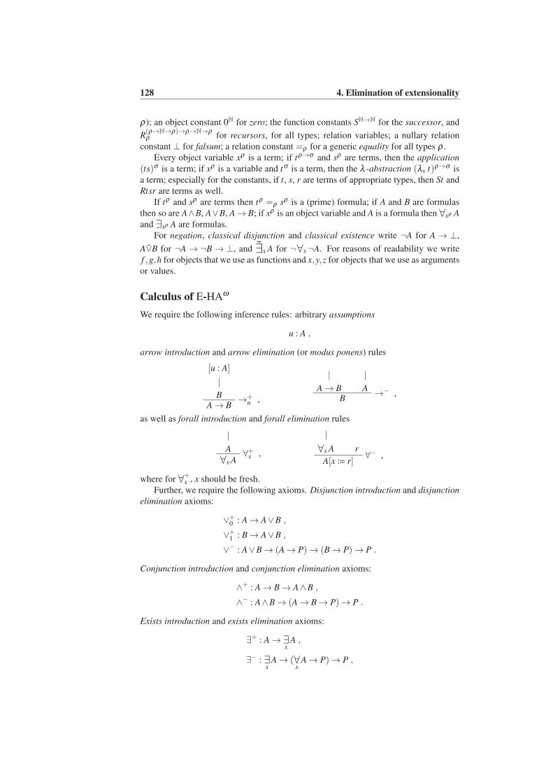
128 4. Elimination of extensionality
ρ); an object constant 0N for zero; the function constants SN→N for the successor, and
R(ρ→N→ρ)→ρ→N→ρρ for recursors, for all types; relation variables; a nullary relation
constant ⊥ for falsum; a relation constant =ρ for a generic equality for all types ρ .
Every object variable xρ is a term; if tρ→σ and sρ are terms, then the application
(ts)σ is a term; if xρ is a variable and tσ is a term, then the λ -abstraction (λx t)ρ→σ is
a term; especially for the constants, if t, s, r are terms of appropriate types, then St and
Rtsr are terms as well.
If tρ and sρ are terms then tρ =ρ sρ is a (prime) formula; if A and B are formulas
then so are A∧B, A∨B, A→ B; if xρ is an object variable and A is a formula then ∀xρ A
and ∃xρ A are formulas.
For negation, classical disjunction and classical existence write ¬A for A → ⊥,
A∨B for ¬A → ¬B →⊥, and ∃x A for ¬∀x¬A. For reasons of readability we write
f ,g,h for objects that we use as functions and x,y,z for objects that we use as arguments
or values.
Calculus of E-HAω
We require the following inference rules: arbitrary assumptions
u : A ,
arrow introduction and arrow elimination (or modus ponens) rules
[u : A]
|
B →+u ,
A→ B
|
A→ B
|
A→− ,
B
as well as forall introduction and forall elimination rules
|
A ∀+x ,∀x A
|
∀x A r∀− ,
A[x≔ r]
where for ∀+x , x should be fresh.
Further, we require the following axioms. Disjunction introduction and disjunction
elimination axioms:
∨+0 : A→ A∨B ,
∨+1 : B→ A∨B ,
∨− : A∨B→ (A→ P)→ (B→ P)→ P .
Conjunction introduction and conjunction elimination axioms:
∧+ : A→ B→ A∧B ,
∧− : A∧B→ (A→ B→ P)→ P .
Exists introduction and exists elimination axioms:
∃+ : A→ ∃x
A ,
∃− : ∃x
A→ (∀x
A→ P)→ P ,
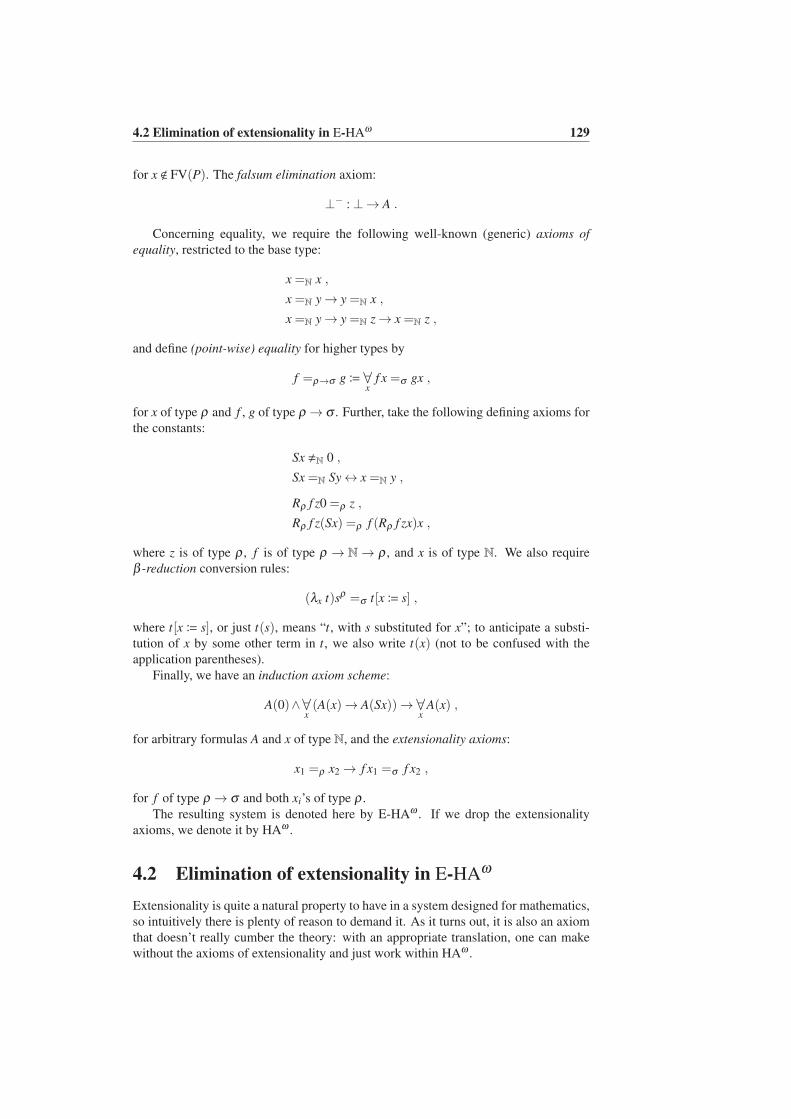
4.2 Elimination of extensionality in E-HAω 129
for x < FV(P). The falsum elimination axiom:
⊥− :⊥→ A .
Concerning equality, we require the following well-known (generic) axioms of
equality, restricted to the base type:
x =N x ,
x =N y→ y =N x ,
x =N y→ y =N z→ x =N z ,
and define (point-wise) equality for higher types by
f =ρ→σ g≔ ∀x
f x =σ gx ,
for x of type ρ and f , g of type ρ → σ . Further, take the following defining axioms for
the constants:
Sx ,N 0 ,
Sx =N Sy↔ x =N y ,
Rρ f z0 =ρ z ,
Rρ f z(Sx) =ρ f (Rρ f zx)x ,
where z is of type ρ , f is of type ρ → N→ ρ , and x is of type N. We also require
β -reduction conversion rules:
(λx t)sρ =σ t[x≔ s] ,
where t[x≔ s], or just t(s), means “t, with s substituted for x”; to anticipate a substi-
tution of x by some other term in t, we also write t(x) (not to be confused with the
application parentheses).
Finally, we have an induction axiom scheme:
A(0)∧∀x(A(x)→ A(Sx))→ ∀
xA(x) ,
for arbitrary formulas A and x of type N, and the extensionality axioms:
x1 =ρ x2 → f x1 =σ f x2 ,
for f of type ρ → σ and both xi’s of type ρ .
The resulting system is denoted here by E-HAω . If we drop the extensionality
axioms, we denote it by HAω .
4.2 Elimination of extensionality in E-HAω
Extensionality is quite a natural property to have in a system designed for mathematics,
so intuitively there is plenty of reason to demand it. As it turns out, it is also an axiom
that doesn’t really cumber the theory: with an appropriate translation, one can make
without the axioms of extensionality and just work within HAω .
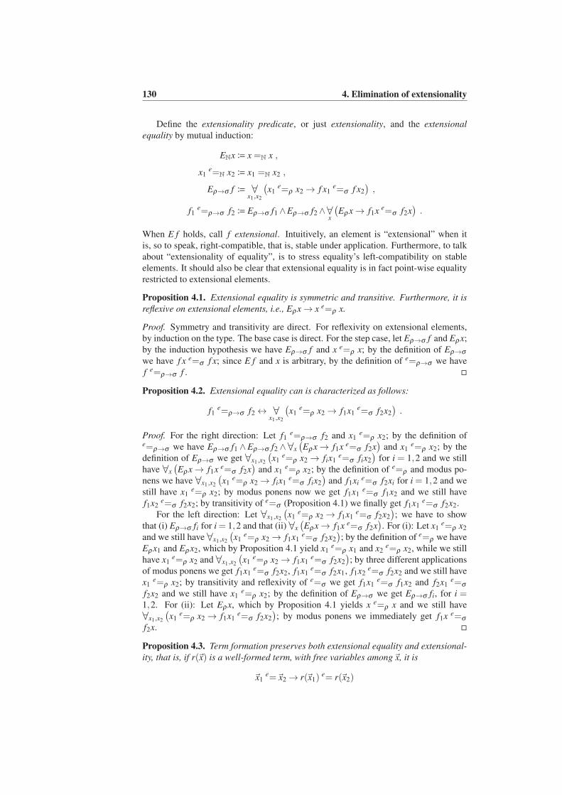
130 4. Elimination of extensionality
Define the extensionality predicate, or just extensionality, and the extensional
equality by mutual induction:
ENx≔ x =N x ,
x1e=N x2 ≔ x1 =N x2 ,
Eρ→σ f ≔ ∀x1,x2
(
x1e=ρ x2 → f x1
e=σ f x2
)
,
f1e=ρ→σ f2 ≔ Eρ→σ f1∧Eρ→σ f2∧∀
x
(
Eρ x→ f1x e=σ f2x)
.
When E f holds, call f extensional. Intuitively, an element is “extensional” when it
is, so to speak, right-compatible, that is, stable under application. Furthermore, to talk
about “extensionality of equality”, is to stress equality’s left-compatibility on stable
elements. It should also be clear that extensional equality is in fact point-wise equality
restricted to extensional elements.
Proposition 4.1. Extensional equality is symmetric and transitive. Furthermore, it is
reflexive on extensional elements, i.e., Eρ x→ x e=ρ x.
Proof. Symmetry and transitivity are direct. For reflexivity on extensional elements,
by induction on the type. The base case is direct. For the step case, let Eρ→σ f and Eρ x;
by the induction hypothesis we have Eρ→σ f and x e=ρ x; by the definition of Eρ→σ
we have f x e=σ f x; since E f and x is arbitrary, by the definition of e=ρ→σ we have
f e=ρ→σ f .
Proposition 4.2. Extensional equality can is characterized as follows:
f1e=ρ→σ f2 ↔ ∀
x1,x2
(
x1e=ρ x2 → f1x1
e=σ f2x2
)
.
Proof. For the right direction: Let f1e=ρ→σ f2 and x1
e=ρ x2; by the definition ofe=ρ→σ we have Eρ→σ f1 ∧Eρ→σ f2 ∧∀x
(
Eρ x→ f1x e=σ f2x)
and x1e=ρ x2; by the
definition of Eρ→σ we get ∀x1,x2
(
x1e=ρ x2 → fix1
e=σ fix2
)
for i = 1,2 and we still
have ∀x
(
Eρ x→ f1x e=σ f2x)
and x1e=ρ x2; by the definition of e=ρ and modus po-
nens we have ∀x1,x2
(
x1e=ρ x2 → fix1
e=σ fix2
)
and f1xie=σ f2xi for i = 1,2 and we
still have x1e=ρ x2; by modus ponens now we get f1x1
e=σ f1x2 and we still have
f1x2e=σ f2x2; by transitivity of e=σ (Proposition 4.1) we finally get f1x1
e=σ f2x2.
For the left direction: Let ∀x1,x2
(
x1e=ρ x2 → f1x1
e=σ f2x2
)
; we have to show
that (i) Eρ→σ fi for i = 1,2 and that (ii) ∀x
(
Eρ x→ f1x e=σ f2x)
. For (i): Let x1e=ρ x2
and we still have ∀x1,x2
(
x1e=ρ x2 → f1x1
e=σ f2x2
)
; by the definition of e=ρ we have
Eρ x1 and Eρ x2, which by Proposition 4.1 yield x1e=ρ x1 and x2
e=ρ x2, while we still
have x1e=ρ x2 and ∀x1,x2
(
x1e=ρ x2 → f1x1
e=σ f2x2
)
; by three different applications
of modus ponens we get f1x1e=σ f2x2, f1x1
e=σ f2x1, f1x2e=σ f2x2 and we still have
x1e=ρ x2; by transitivity and reflexivity of e=σ we get f1x1
e=σ f1x2 and f2x1e=σ
f2x2 and we still have x1e=ρ x2; by the definition of Eρ→σ we get Eρ→σ fi, for i =
1,2. For (ii): Let Eρ x, which by Proposition 4.1 yields x e=ρ x and we still have
∀x1,x2
(
x1e=ρ x2 → f1x1
e=σ f2x2
)
; by modus ponens we immediately get f1x e=σ
f2x.
Proposition 4.3. Term formation preserves both extensional equality and extensional-
ity, that is, if r(~x) is a well-formed term, with free variables among~x, it is
~x1e=~x2 → r(~x1)
e= r(~x2)
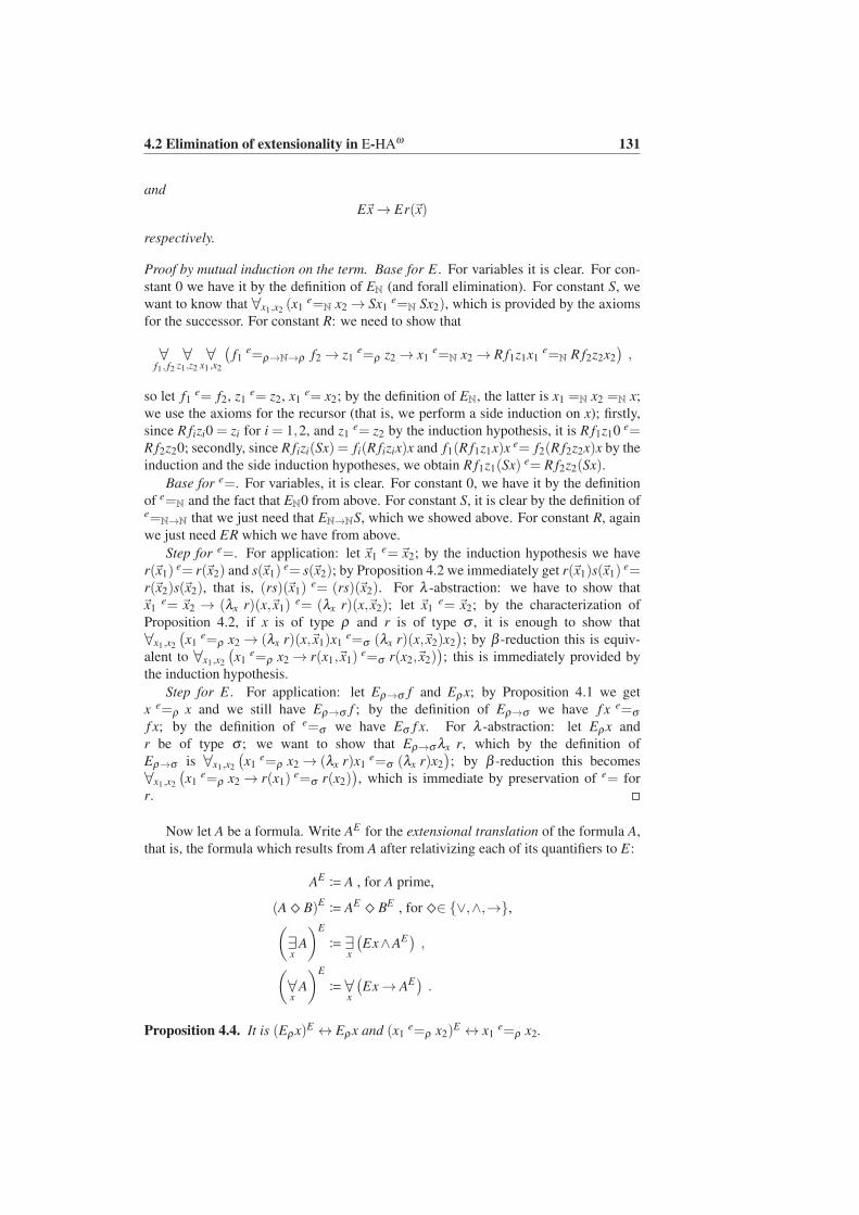
4.2 Elimination of extensionality in E-HAω 131
and
E~x→ Er(~x)
respectively.
Proof by mutual induction on the term. Base for E. For variables it is clear. For con-
stant 0 we have it by the definition of EN (and forall elimination). For constant S, we
want to know that ∀x1,x2(x1
e=N x2 → Sx1e=N Sx2), which is provided by the axioms
for the successor. For constant R: we need to show that
∀f1, f2
∀z1,z2
∀x1,x2
(
f1e=ρ→N→ρ f2 → z1
e=ρ z2 → x1e=N x2 → R f1z1x1
e=N R f2z2x2
)
,
so let f1e= f2, z1
e= z2, x1e= x2; by the definition of EN, the latter is x1 =N x2 =N x;
we use the axioms for the recursor (that is, we perform a side induction on x); firstly,
since R fizi0 = zi for i = 1,2, and z1e= z2 by the induction hypothesis, it is R f1z10 e=
R f2z20; secondly, since R fizi(Sx) = fi(R fizix)x and f1(R f1z1x)x e= f2(R f2z2x)x by the
induction and the side induction hypotheses, we obtain R f1z1(Sx) e= R f2z2(Sx).
Base for e=. For variables, it is clear. For constant 0, we have it by the definition
of e=N and the fact that EN0 from above. For constant S, it is clear by the definition ofe=N→N that we just need that EN→NS, which we showed above. For constant R, again
we just need ER which we have from above.
Step for e=. For application: let ~x1e=~x2; by the induction hypothesis we have
r(~x1)e= r(~x2) and s(~x1)
e= s(~x2); by Proposition 4.2 we immediately get r(~x1)s(~x1)e=
r(~x2)s(~x2), that is, (rs)(~x1)e= (rs)(~x2). For λ -abstraction: we have to show that
~x1e= ~x2 → (λx r)(x,~x1)
e= (λx r)(x,~x2); let ~x1e= ~x2; by the characterization of
Proposition 4.2, if x is of type ρ and r is of type σ , it is enough to show that
∀x1,x2
(
x1e=ρ x2 → (λx r)(x,~x1)x1
e=σ (λx r)(x,~x2)x2
)
; by β -reduction this is equiv-
alent to ∀x1,x2
(
x1e=ρ x2 → r(x1,~x1)
e=σ r(x2,~x2))
; this is immediately provided by
the induction hypothesis.
Step for E. For application: let Eρ→σ f and Eρ x; by Proposition 4.1 we get
x e=ρ x and we still have Eρ→σ f ; by the definition of Eρ→σ we have f x e=σ
f x; by the definition of e=σ we have Eσ f x. For λ -abstraction: let Eρ x and
r be of type σ ; we want to show that Eρ→σ λx r, which by the definition of
Eρ→σ is ∀x1,x2
(
x1e=ρ x2 → (λx r)x1
e=σ (λx r)x2
)
; by β -reduction this becomes
∀x1,x2
(
x1e=ρ x2 → r(x1)
e=σ r(x2))
, which is immediate by preservation of e= for
r.
Now let A be a formula. Write AE for the extensional translation of the formula A,
that is, the formula which results from A after relativizing each of its quantifiers to E:
AE≔ A , for A prime,
(A ^ B)E≔ AE
^ BE , for ^∈ ∨,∧,→,(
∃x
A
)E
≔ ∃x
(
Ex∧AE)
,
(
∀x
A
)E
≔ ∀x
(
Ex→ AE)
.
Proposition 4.4. It is (Eρ x)E ↔ Eρ x and (x1e=ρ x2)
E ↔ x1e=ρ x2.
132 4. Elimination of extensionality
Proof by mutual induction on the type. Base: Immediate from the definition of
EN and e=N. Step for E: Let (Eρ→σ f )E , which by definition means(
∀x1,x2
(
x1e=ρ x2 → f x1
e=σ f x2
))E; by the definition of the extensional translation,
this is equivalent to ∀x1,x2
(
Eρ x1∧Eρ x2 → (x1e=ρ x2)
E → ( f x1e=σ f x2)
E)
, where
the first two clauses are redundant; the induction hypothesis for e= yields equiva-
lently ∀x1,x2
(
x1e=ρ x2 → f x1
e=σ f x2
)
, which, by the definition of Eρ→σ , is Eρ→σ f .
Step for e=: Let ( f1e=ρ→σ f2)
E ; by the definition of e=ρ→σ , this is equivalent to(
Eρ→σ f1∧Eρ→σ f2∧∀x
(
Eρ x→ f1x e=σ f2x))E
; by the definition of the extensional
translation, this is equivalent to (Eρ→σ f1)E ∧ (Eρ→σ f2)
E ∧∀x
(
Eρ x→ f1x e=σ f2x)
;
by the step for E, we get the equivalent Eρ→σ f1∧Eρ→σ f2∧∀x
(
Eρ x→ f1x e=σ f2x)
,
which is by definition equivalent to f1e=ρ→σ f2.
Proposition 4.5. Point-wise equality is equivalent to extensional equality up to exten-
sional translation, that is,
(
Eρ x1 → Eρ x2 → (x1 =ρ x2)E)
↔ x1e=ρ x2 .
Proof by induction on the type. Base: Immediate. Step: Let Eρ→σ f1 ∧ Eρ→σ f2 ∧( f1 =ρ→σ f2)
E ; by the definition of =ρ→σ we have Eρ→σ f1 ∧Eρ→σ f2 ∧ (∀x f1x =σ
f2x)E ; by the definition of the extensional translation we have Eρ→σ f1 ∧Eρ→σ f2 ∧
∀x
(
Eρ x→ ( f1x =σ f2x)E)
; by preservation of extensionality (Proposition 4.3) we can
write Eρ→σ f1 ∧Eρ→σ f2 ∧∀x
(
Eρ x→ Eσ f1x∧Eσ f2x∧ ( f1x =σ f2x)E)
; by the induc-
tion hypothesis for type σ we get Eρ→σ f1∧Eρ→σ f2∧∀x
(
Eρ x→ f1x e=σ f2x)
, which
by the definition of e=ρ→σ is precisely f1e=ρ→σ f2.
Theorem 4.6 (Elimination of extensionality). The formula A(~x) is derivable within
E-HAω from assumptions ui : Ai(~xi) if and only if the formula E(~x)→ AE(~x) is deriv-
able within HAω from assumptions uEi : E~xi → AE
i (~xi).
Proof by induction on the calculus. We argue informally for the right (“only-if”) di-
rection, which is the most important.
Leaf cases. For assumptions it is trivial. Moreover, since extensional translation af-
fects only those formulas where quantification appears, it is trivial to prove the axioms
∨+, ∨−, ∧+, ∧−, ⊥−, as well as the ones for the recursor and β -reduction. Then, the
axioms of equality and the successor deal with prime formulas and are also trivial.
For exists introduction: For a formula A(x,~x), we have to show that Ex∧E~x →
(A→ ∃x A)E; use ∃+ for the formula Ex∧AE .
For exists elimination: For formulas A(x,~x) and B(~y) with x not among~y, we have
to show that Ex∧ E~x∧ E~y → ((∀x A→ B)→ ∃x A→ B)E; use ∃− for the formulas
Ex∧AE , BE .
For induction axioms: For a formula A(x,~x), we have to show that Ex∧ E~x →
(A(0,~x)→ ∀x (A(x,~x)→ A(Sx,~x))→ ∀x A(x,~x))E; use IndN for the formula Ex →
A(x,~x).
For extensionality axioms: We have to show that Eρ x1 ∧ Eρ x2 ∧ Eρ→σ f1 ∧Eρ→σ f2 → (x1 =ρ x2 → f1x1 =σ f2x2)
E , that is, Eρ x1∧Eρ x2∧Eρ→σ f1∧Eρ→σ f2 →(x1 =ρ x2)
E → ( f1x1 =σ f2x2)E ; by preservation of extensionality (Proposition 4.3)
we get Ex1 ∧Ex2 ∧Eσ f1x1 ∧Eσ f2x2 → (x1 =ρ x2)E → ( f1x1 =σ f2x2)
E ; by Propo-
sition 4.5, we get x1e=ρ x2 → f1x1
e=σ f2x2, or, equivalently by Proposition 4.2,
f1e=ρ→σ f2, which is an atomic formula within HAω .
4.3 Notes 133
Step cases. For arrow introduction: Let E~y → BE(~y), derived from assumption
E~x→ AE(~x), be the premise; we want to derive E~x∧E~y→ AE(~x)→ BE(~y); so suppose
E~x, E~y, AE and show BE ; use→+ for the formulas AE and BE .
For arrow elimination: Let E~x∧ E~y → AE(~x)→ BE(~y) and E~x → AE(~x) be the
premise; we want to derive E~y→ BE(~y); so suppose E~y and show BE(~y); use →− for
the formulas AE → BE and AE .
For forall introduction: Let Ex∧E~x→ AE(x,~x) be the premise; we want to derive
E~x→ ∀x
(
Ex→ AE)
; so suppose E~x and show ∀x
(
Ex→ AE)
; use ∀+ for the formula
Ex→ AE(x,~x).For forall elimination: Let E~x → ∀x
(
Ex→ AE(x,~x))
and r(~y) be the premise,
where r is a term of the same type as x; we want to derive E~x∧ E~y → AE [x ≔ r];so suppose E~x and E~y and show AE [x ≔ r]; use ∀− for the formula AE(x,~x) and the
variable x, where extensionality is preserved by Proposition 4.3.
4.3 Notes
Dues
The arguments of this chapter were devised under the guidance of Helmut Schwichten-
berg in 2006, and carried through in juxtaposition to the exposition of Horst Luckhardt
in [28] and its simplification by Ulrich Kohlenbach in an earlier draft of [22]; both of
these are based on Robin Gandy’s [12], while Luckhardt further reports that elimina-
tion of extensionality by relativization is to be found in Gaisi Takeuti’s [53] (earlier
than Gandy’s seemingly independent effort) as well as in Kurt Schutte’s [43]. In an-
other direction, elimination of extensionality in Martin-Lof type theory is the subject
of Martin Hofmann’s [15] (see also [16]).
Outlook
Elimination of extensionality as we presented it will find its place within TCF+ as soon
as the latter matures enough to formally encompass Heyting arithmetic; an embedding
of Heyting arithmetic into TCF+ is a straightforward and early question to pursue while
developing TCF+.

Appendix A
Some domain theory
We collect here notions and statements from elementary domain theory which are used
in the text as known facts. For details one can look into [52, 1, 2].
Preordered and ordered sets
Let T be a set with equality1 and ≥ a binary relation on T . The relation ≥ is well-
founded if there is no infinite sequence of the sort x0 ≥ x1 ≥ ·· · in T . It is finitely
branching if the class y ∈ T | x≥ y is finite for every x ∈ T . Say that y ∈ T is an
immediate successor of x ∈ T if it is
x≥ y∧ ∀w∈T
((x≥ w→ y≥ w)∧ (w≥ y→ w≥ x)) ,
and write x ≥1 y (note that it is also x ≥1 x). The relation ≥ is finitarily branching (or
locally finitely branching) if the set of immediate successors x≥1 ≔ y ∈ T | x≥1 y is
finite for every x ∈ T .
The couple (T,≥) is a preordered set if≥ is reflexive and transitive and a (partially)
ordered set (or poset) if ≥ is reflexive, transitive and antisymmetric.
Fact A.1. A preordered set (T,≥) induces an ordered set (T/∼,≥), where
a∼ b⇔ a≥ b∧b≥ a
A maximal element a in a preordered set (T,≥) is such that ∀b∈T (b≥ a→ b≡ a);dually, a minimal element a is such that ∀b∈T (a≥ b→ a≡ b). Denote the set of max-
imal elements of T by mxlT . A least element (or minimum)⊥ is such that ∀a∈T a≥⊥.
An upper bound of a subset ai is an element a ∈ T such that ∀i a ≥ ai; a is a least
upper bound (or supremum) if
∀i
a≥ ai ∧ ∀i
b≥ ai → b≥ a ;
write a = lubiai. Call a,b ∈ T consistent if they have a common upper bound. We
remark the following:
1. Least elements of T or least upper bounds of an arbitrary subset of T , don’t have
to exist, but, in case T is an ordered set, if they do, they are unique.
1Say that a set T is a set with equality if it is equipped with an equivalence relation ≡T .
136 A. Some domain theory
2. Let S⊆ T , where T is an ordered set. Concerning the cardinality of the set mxlS,
we have the following possible cases:
(a) It may be empty; for example, consider S being an infinite ascending chain.
(b) It may be finite; this is the case with S being a singleton, or a discrete
subset (that is, consisting of mutually incomparable elements), or, say, a
finite (therefore finitely branching) tree.
(c) It may be infinite; for example, take S to be an infinitely branching flat tree.
Fact A.2. Let (T,≥) be an ordered set, U ⊆ T a subset and U ′ ⊆U such that
∀a∈U
∃a′∈U ′
a′ ≥ a .
The least upper bound of U exists if and only if the least upper bound of U ′ exists and,
if it does, lubU = lubU ′.
Let (T,≥) be an ordered set. A subset U ⊆ T is (upwards) directed when every
two of its elements have a common upper bound in U , that is,
∀a1,a2∈U
∃a∈U
(a≥ a1∧a≥ a2) .
Write U ∈Pd(T ) and U ⊆d T . Further, U is closed (under the order) when
a ∈U ∧a≥ a′→ a′ ∈U .
Fact A.3. Let (T,≥) be an ordered set.
1. Let U ⊆ T . The closure U ≔ a ∈ T | ∃a′∈U a′ ≥ a is the smallest closed set in
(T,≥) that contains U.
2. For every a ∈ T , the closure a is a directed set.
A pre-ordered set (T,≥) is complete when every subset has a least upper bound,
δ -complete if every directed subset has a least upper bound, ω-complete when it has
a least element and every denumerable directed subset has a least upper bound, and
consistently complete when every consistent pair has a least upper bound; note that, in
the case of an ordered set, all of these least upper bounds are unique. Call the relation
≥ well-ordered if it yields no infinite descending chains in T , that is,
∀ann∈N⊆T
(
∀n∈N
an ≥ an+1 → ∃n0∈N
∀n≥Nn0
an ≡ an0
)
.
Fact A.4. An ordered set (T,≥) with a least element is ω-complete if and only if every
increasing sequence in it has a least upper bound.
An order-preserving mapping f from an ordered set (T,≥) to an ordered set
(T ′,≥′), is a mapping f : T → T ′ for which
a≥ b→ f (a)≥′ f (b)
If both (T,≥), (T ′,≥′) are complete, δ -complete or ω-complete then an order-
preserving mapping from one to the other is continuous, δ -continuous or ω-continuous
if it commutes with supremums of subsets, directed subsets or denumerable directed
subsets respectively:
f (lubU) = lub f (U)
where f (U)≔ f (a) ∈ T ′ | a ∈U.
137
Fact A.5. Let (T,≥), (T ′,≥′) be ω-complete ordered sets. An order-preserving map-
ping f : T → T ′ is ω-complete if and only if it commutes with supremums of increasing
sequences in T .
Domains
We restrict our attention to δ -complete ordered sets with least element, which we just
call complete ordered sets, or cpo’s, and we interpret a ≥ b as “a is approximated by
b”. For a detailed exposition we refer to [52, §§3.1–2].
Let D = (T,≥,⊥) be a cpo. Define its compact (or finite) elements by
a ∈ Dc ≔ ∀U⊆dT
(
lubU ≥ a→ ∃b∈U
b≥ a
)
.
So compact elements are those which, whenever they approximate the least upper
bound of a directed set U , they do so with a witness b ∈ U . Let apx(a) denote the
set of compact approximations of a, that is, apx(a)≔ b ∈ Dc | a≥ b. The cpo D is
called algebraic if every element a ∈ T can be characterized by its compact approxi-
mations, that is, if
∀a∈T
(apx(a) ∈Pd(T )∧a = lubapx(a)) .
Finally, an algebraic cpo D = (T,≥,⊥) is called a (Scott-Ershov) domain when every
pair of consistent compact elements has a least upper bound (not necessarily compact
itself), that is, when
∀a,b∈Dc
(
∃c∈T
(c≥ a∧ c≥ b)→ luba,b ∈ T
)
.
Fact A.6. Let D = (T,≥,⊥) be an algebraic cpo. The following hold.
1. For all a,b ∈ T it is a≥ b if and only if apx(a)≥ apx(b).
2. If U ⊆d T then apx(lubU) =⋃
a∈U apx(a).
Fact A.7. Let D = (T,≥,⊥) be an algebraic cpo and D′ = (T ′,≥′,⊥′) a cpo. The
following hold.
1. A mapping f : D → D′ is continuous if and only if f (a) = lub f (b)b∈apx(a),
for all a ∈ T . Moreover, every monotone function f : Dc → D′ has a unique
continuous extension f : D→ D′ given by f (a)≔ lub f (b)b∈apx(a).
2. Let D′ be algebraic as well and f : D→ D′. Then f is continuous if and only if
it is monotone and it satisfies the principle of finite support, that is,
∀a∈D
(
b ∈ apx( f (a))→ ∃c∈apx(a)
f (c)≥ b
)
.
Fact A.8. Let D be a domain.
1. If U ⊆ f Dc is consistent, that is, if it has an upper bound, then it has a compact
least upper bound lubU ∈ Dc.
138 A. Some domain theory
2. Every domain is consistently complete, that is, every upper bounded set has a
least upper bound.
An ideal u in a domain D = (T,≥,⊥) is a set u⊆ Dc which contains the least ele-
ment, is downwards closed and consistently complete, that is, it satisfies the following:
• ⊥ ∈ u
• a ∈ u∧a≥ b→ b ∈ u
• ∀a,b∈u luba,b ∈ u
Let a≔ b ∈ Dc | a≥ b and write IdeD to denote the set of ideals in D.
Fact A.9 (First Representation Theorem). The triple Dc ≔ (IdeD,⊇,⊥) constitutes a
domain. Moreover, it is Dc D, through the mapping u 7→ lubu.
The domain Dc is called the ideal completion of Dc.
Bibliography
[1] Samson Abramsky and Achim Jung. Domain theory. In Handbook of logic in computer science, Vol.
3, volume 3 of Handb. Log. Comput. Sci., pages 1–168. Oxford Univ. Press, New York, 1994. (Cited
on pages 125 and 135.)
[2] Roberto M. Amadio and Pierre-Louis Curien. Domains and lambda-calculi, volume 46 of Cambridge
Tracts in Theoretical Computer Science. Cambridge University Press, Cambridge, 1998. (Cited on
page 135.)
[3] Holger Benl, Ulrich Berger, Helmut Schwichtenberg, Monika Seisenberger, and Wolfgang Zuber.
Proof theory at work: Program development in the MINLOG system. In W. Bibel and P.H. Schmitt,
editors, Automated Deduction — A Basis for Applications, Volume II Systems and Implementation.
Kluwer, 1998. (Cited on page 103.)
[4] Ulrich Berger. Totale Objekte und Mengen in der Bereichstheorie. PhD thesis, Mathematisches Institut
der Universitat Munchen, 1990. (Cited on page 103.)
[5] Ulrich Berger. Total sets and objects in domain theory. Ann. Pure Appl. Logic, 60(2):91–117, 1993.
(Cited on page 103.)
[6] Ulrich Berger, Kenji Miyamoto, Helmut Schwichtenberg, and Monika Seisenberger. MINLOG — a
tool for program extraction supporting algebras and coalgebras. In Andrea Corradini, Bartek Klin, and
Corina Cırstea, editors, CALCO, volume 6859 of Lecture Notes in Computer Science, pages 393–399.
Springer, 2011. (Cited on page 103.)
[7] Douglas S. Bridges and Luminita S. Vıta. Apartness and Uniformity. Theory and Applications of
Computability. Springer, 2011. (Cited on page 126.)
[8] Antonio Bucciarelli, Alberto Carraro, Thomas Ehrhard, and Antonino Salibra. On linear information
systems. In LINEARITY, pages 38–48, 2009. (Cited on page 46.)
[9] Thierry Coquand, Giovanni Sambin, Jan Smith, and Silvio Valentini. Inductively generated formal
topologies. Ann. Pure Appl. Logic, 124(1-3):71–106, 2003. (Cited on page 113.)
[10] Yuri L. Ershov. Maximal and everywhere-defined functionals. Algebra and Logic, 13:210–225, 1974.
(Cited on page 102.)
[11] Martın Hotzel Escardo. PCF extended with real numbers: a domain-theoretic approach to higher-
order exact real number computation. PhD thesis, University of London, Imperial College of Science,
Technology and Medicine, Department of Computing, 1997. (Cited on page 34.)
[12] Robin O. Gandy. On the axiom of extensionality—Part I. J. Symb. Log., 21(1):36–48, 1956. (Cited on
pages 4 and 133.)
[13] Gerhard Gierz, Karl Heinrich Hofmann, Klaus Keimel, Jimmie D. Lawson, Michael Mislove, and
Dana S. Scott. Continuous Lattices and Domains, volume 93 of Encyclopedia of Mathematics and its
Applications. Cambridge University Press, 2003. (Cited on page 20.)
[14] Jean-Yves Girard, Paul Taylor, and Yves Lafont. Proofs and types, volume 7 of Cambridge Tracts in
Theoretical Computer Science. Cambridge University Press, Cambridge, 1989. (Cited on page 125.)
[15] Martin Hofmann. Elimination of extensionality in Martin-Lof type theory. In Types for proofs and
programs (Nijmegen, 1993), volume 806 of Lecture Notes in Comput. Sci., pages 166–190. Springer,
Berlin, 1994. (Cited on page 133.)
[16] Martin Hofmann. Extensional concepts in intensional type theory. PhD thesis, University of Edinburgh,
1995. (Cited on page 133.)
[17] William A. Howard. Appendix: Hereditarily majorizable functionals of finite type. In Troelstra [55],
pages 454–461. Lecture Notes in Mathematics, Vol. 344. (Cited on page 127.)
140 BIBLIOGRAPHY
[18] Simon Huber, Basil A. Karadais, and Helmut Schwichtenberg. Towards a formal theory of com-
putability. In Ways of Proof Theory (Pohler’s Festschrift), pages 257–282. Ontos Verlag, Frankfurt,
2010. (Cited on pages 4, 47, 100, 103, and 127.)
[19] David S. Johnson, Christos H. Papadimitriou, and Mihalis Yannakakis. On generating all maximal
independent sets. Inf. Process. Lett., 27(3):119–123, 1988. (Cited on page 101.)
[20] Peter T. Johnstone. Stone spaces, volume 3 of Cambridge Studies in Advanced Mathematics. Cam-
bridge University Press, Cambridge, 1982. (Cited on page 125.)
[21] Stephen C. Kleene. Countable functionals. In Constructivity in mathematics: Proceedings of the
colloquium held at Amsterdam, 1957 (edited by A. Heyting), Studies in Logic and the Foundations
of Mathematics, pages 81–100, Amsterdam, 1959. North-Holland Publishing Co. (Cited on pages 1
and 102.)
[22] Ulrich Kohlenbach. Applied proof theory: proof interpretations and their use in mathematics. Springer
Monographs in Mathematics. Springer-Verlag, Berlin, 2008. (Cited on page 133.)
[23] Georg Kreisel. Wittgenstein’s remarks on the foundations of mathematics. British Journal for the
Philosophy of Science, 9(34):135–158, 1958. (Cited on page x.)
[24] Georg Kreisel. Interpretation of analysis by means of constructive functionals of finite types. In
Constructivity in mathematics: Proceedings of the colloquium held at Amsterdam, 1957 (edited by A.
Heyting), Studies in Logic and the Foundations of Mathematics, pages 101–128, Amsterdam, 1959.
North-Holland Publishing Co. (Cited on pages 1 and 102.)
[25] Lill Kristiansen and Dag Normann. Total objects in inductively defined types. Archive for Mathemati-
cal Logic, 36:405–436, 1997. (Cited on page 103.)
[26] Thomas S. Kuhn. The structure of scientific revolutions. University of Chicago Press, Chicago, 1970.
(Cited on page x.)
[27] Imre Lakatos. Proofs and refutations: the logic of mathematical discovery. Cambridge University
Press, 12th edition, 1976. (Cited on page x.)
[28] Horst Luckhardt. Extensional Godel functional interpretation. A consistency proof of classical anal-
ysis. Lecture Notes in Mathematics. 306. Berlin-Heidelberg-New York: Springer-Verlag. VI, 161 p.,
1973. (Cited on page 133.)
[29] George Markowsky and Barry K. Rosen. Bases for chain-complete posets. IBM J. Res. Develop.,
20(2):138–147, 1976. (Cited on page 125.)
[30] Sara Negri. Continuous domains as formal spaces. Math. Structures Comput. Sci., 12(1):19–52, 2002.
(Cited on pages 113, 118, 119, and 125.)
[31] Dag Normann. Computability over the partial continuous functionals. J. Symbolic Logic, 65(3):1133–
1142, 2000. (Cited on page 34.)
[32] Dag Normann. Applications of the Kleene–Kreisel Density Theorem to Theoretical Computer Science.
In S. Barry Cooper, Benedikt Lwe, and Andrea Sorbi, editors, New Computational Paradigms, pages
119–138. Springer New York, 2008. (Cited on page 103.)
[33] Erik Palmgren. A note on domain representability and formal topology. Revised version of U.U.D.M.
Report 2007:28, Department of Mathematics, University of Uppsala, 2007, 2007. (Cited on pages 113
and 124.)
[34] Iosif Petrakis. The topology of the strong Scott condition. Preprint, 2012. (Cited on page 20.)
[35] Gordon D. Plotkin. LCF considered as a programming language. Theoret. Comput. Sci., 5(3):223–255,
1977/78. (Cited on pages 34 and 47.)
[36] Gordon D. Plotkin. T ω as a universal domain. J. Comput. System Sci., 17(2):209–236, 1978. (Cited
on page 125.)
[37] Giovanni Sambin. Intuitionistic formal spaces — a first communication. In Mathematical logic and its
applications (Druzhba, 1986), pages 187–204. Plenum, New York, 1987. (Cited on page 118.)
[38] Giovanni Sambin. Formal topology and domains. In Electronic notes in theoretical computer sci-
ence, 35 (Remagen-Rolandseck, 1998), volume 35 of Electron. Notes Theor. Comput. Sci., page 14 pp.
(electronic). Elsevier, Amsterdam, 2000. (Cited on pages 105 and 113.)
[39] Giovanni Sambin. Some points in formal topology. Theoret. Comput. Sci., 305(1-3):347–408, 2003.
Topology in computer science (Schloß Dagstuhl, 2000). (Cited on pages 113 and 118.)
[40] Giovanni Sambin and Silvia Gebellato. A preview of the basic picture: a new perspective on formal
topology. In Types for proofs and programs (Irsee, 1998), volume 1657 of Lecture Notes in Comput.
Sci., pages 194–207. Springer, Berlin, 1999. (Cited on page 113.)
BIBLIOGRAPHY 141
[41] Giovanni Sambin, Silvio Valentini, and Paolo Virgili. Constructive domain theory as a branch of
intuitionistic pointfree topology. Theoret. Comput. Sci., 159(2):319–341, 1996. (Cited on pages 113
and 125.)
[42] Peter Schuster. Formal Zariski topology: positivity and points. Ann. Pure Appl. Logic, 137(1-3):317–
359, 2006. (Cited on page 113.)
[43] Kurt Schutte. Grundlagen der Analysis im Rahmen einer einfachen Typenlogik: Ausz. (mit einigen
Erg.) aus d. Vorlesung: Grundlagen d. Math., Munchen, W.S. 1966/67. 1967. (Cited on page 133.)
[44] Helmut Schwichtenberg. Eine Normalform fur endliche Approximationen von partiellen stetigen Funk-
tionalen. In J. Diller, editor, Logik und Grundlagenforschung, Festkolloquium zum 100. Geburtstag von
Heinrich Scholz, pages 89–95, 1986. (Cited on page 46.)
[45] Helmut Schwichtenberg. Density and choice for total continuous functionals. In Kreiseliana. About
and Around Georg Kreisel, pages 335–362, 1996. (Cited on page 103.)
[46] Helmut Schwichtenberg. Classifying recursive functions. In E. Griffor, editor, Handbook of com-
putability theory, volume 140 of Stud. Logic Found. Math., pages 533–586. North-Holland, Amster-
dam, 1999. (Cited on pages 34 and 47.)
[47] Helmut Schwichtenberg. Recursion on the partial continuous functionals. In C. Dimitracopoulos,
L. Newelski, D. Normann, and J. Steel, editors, Logic Colloquium ’05, volume 28 of Lecture Notes in
Logic, pages 173–201. Association for Symbolic Logic, 2006. (Cited on pages 3, 5, and 46.)
[48] Helmut Schwichtenberg. MINLOG. In Freek Wiedijk, editor, The Seventeen Provers of the World, vol-
ume 3600 of Lecture Notes in Computer Science, pages 151–157. Springer, 2006. (Cited on page 103.)
[49] Helmut Schwichtenberg and Stanley S. Wainer. Proofs and computations. Perspectives in Logic.
Cambridge University Press, Cambridge, 2012. (Cited on pages 1, 3, 50, 97, and 127.)
[50] Dana S. Scott. A type-theoretical alternative to ISWIM, CUCH, OWHY. Manuscript, 1969. (Cited on
page 1.)
[51] Dana S. Scott. Domains for denotational semantics. In Automata, languages and programming
(Aarhus, 1982), volume 140 of Lecture Notes in Comput. Sci., pages 577–613. Springer, Berlin, 1982.
(Cited on page 108.)
[52] Viggo Stoltenberg-Hansen, Ingrid Lindstrom, and Edward R. Griffor. Mathematical theory of domains,
volume 22 of Cambridge Tracts in Theoretical Computer Science. Cambridge University Press, 1994.
(Cited on pages 103, 113, 114, 115, 117, 118, 119, 125, 135, and 137.)
[53] Gaisi Takeuti. On a generalized logic calculus. Japanese Journal of Mathematics, 23:39–96, 1953.
Errata: ibid, vol. 24 (1954), 149–156. (Cited on page 133.)
[54] Terese. Term rewriting systems, volume 55 of Cambridge Tracts in Theoretical Computer Science.
Cambridge University Press, Cambridge, 2003. (Cited on page 100.)
[55] Anne S. Troelstra, editor. Metamathematical investigation of intuitionistic arithmetic and analysis.
Springer-Verlag, Berlin, 1973. Lecture Notes in Mathematics, Vol. 344. (Cited on pages 127 and 139.)
[56] Wolfgang Wechler. Universal algebra for computer scientists, volume 25 of EATCS Monographs on
Theoretical Computer Science. Springer-Verlag, Berlin, 1992. (Cited on page 2.)
[57] Glynn Winskel. Event structures. In Advances in Petri nets 1986, Part II (Bad Honnef, 1986), volume
255 of Lecture Notes in Comput. Sci., pages 325–392. Springer, Berlin, 1987. (Cited on page 126.)
[58] Ludwig Wittgenstein. Bemerkungen uber die Grundlagen der Mathematik. Suhrkamp, Frankfurt am
Main, 1984. (Cited on page x.)

Index
aboveness, 31
Abramsky, Samson, 125
acis, 3, 7, 47, 49, 53, 84
algebraic, 29
antisymmetric, 32
arithmetical, 31, 34
basic algebraic, 29, 62
composite algebraic, 29
induced by algebra, 29
matrix, 53
nbr-acis, 56, 60, 100
parametric, 32
sub-acis, 8
acis graph, 6
Alexandrov topology, 19
algebra, 1
comparability, 46
finitary, 1, 82
infinitary, 2, 48, 85
non-superunary, 3, 34, 46, 51, 126
structure-finitary, 1
apartness space, 126
application, 17
boolean, 87
of constructor contexts to matrices, 66, 67
of constructors to matrices, 63
of ideals, 23, 34
of lists, 50, 88
of sets, 17
approximable map, 107, 114
n-ary, 29
of acises, 17
of precusl’s, 116
of Scott–Ershov formal topologies, 121
argument
parametric, 1
recursive, 1
arity
left arity of a constructor context, 66
of a constructor, 1
right arity of a constructor context, 66
atom, 7
atomicity, 111, 124
as uniformity, 101
implicit, 3, 48, 51, 94, 101, 126
B, 2, 3, 30
basic coefficient of a matrix, 77, 86
basis of a matrix, 77, 86
Berger, Ulrich, 46, 103
block coding, 57
blocking and unblocking, 57
Bridges, Douglas, ix
category of ideals, 26
CiE 2008, 47
closure-mapping, 13
coherence, 6, 49, 111, 113
coherence space, 125
coherent locale, 125
compact approximation, 114, 137
comparability property, 31, 44, 47
composition of ideals, 26, 34
conditional extension functional, 38, 47
conditional functional, 37
cone of ideals, 7, 20
conjunction functional, 37
conjunction-implication information system, 51, 100
consistency, 3, 7, 135, 137
head-consistency, 69
left-consictency, 94
of constructor contexts, 68
of matrices, 53, 56
propagation of, 6, 49, 106
trivial, 89
consistent set, 7
consistently defined, 17
constructor, 1
partiality pseudo-constructor, 2, 28, 50
proper, 50
constructor arity, 1
constructor context, 66
constructor operator, 63
constructor context, 66
blank, 66
identity, 66
continuous union functional, 47
Coquand counterexample, 47, 67, 89, 106, 113, 125
Coquand information system, 106, 113
Coquand, Thierry, x, 47, 125
cpo, 137
currying functional, 25, 34
D, 51
deductive closure, 7, 106, 136
definability, 34, 48
Dialectica realizability, 127
disjoint union of acises, 8
144 INDEX
disjunction functional, 37
domain, 114, 137
coherent, 114
continuous, 125
domain ideal, 138
domain theory, 1, 113
E-HAω , 127
eigen-neighborhood, 94, 126
eigensplitting mapping, 96
eigentoken, 82
eigenvector, 82
entailment, 3, 7, 44, 50, 63, 88, 105
contravariance of, 90
of constructor contexts, 68
of matrices, 53, 57
enumeration functional, 38
equality
extensional equality, 130
ideal-wise, 108
of neighborhoods, 29
of tokens, 28
point-wise, 129, 130, 132
equientailment, 78, 95, 109
atomical equientailment, 78
equivalence, 78, 109
atomical, 78
Ershov, Yuri, 102
evaluation functional, 25, 34
event structure, 126
existential functional, 36
extension lemma, 97
extensionality, 127
factorization, 67, 78, 80, 85, 87
flattening mapping, 93, 96
formal point, 118
formal topology, 105, 113, 118
coherent Scott–Ershov, 123
consistently complete, 119
Scott–Ershov, 119
unary, 119, 124
function space, 1
atomic, 56
of acises, 10
functional, 1
arithmetical, 30
computable, 34
continuous, 31
extensional, 130
partial, 1
recursive in pcond, exist, and condext, 42
total, 1, 97
Gandy, Robin, 4, 133
Girard, Jean-Yves, 125
HAω , 127
Hausdorff space, 19
higher-type computability, 1, 127
Hofmann, Martin, x, 133
homogenization
of matrices, 73
of tokens, 69, 86
Howard, William, 127
Huber, Simon, ix, 47
ideal, 7, 106
cone, 7, 20
empty, 7, 23
finitely valued, 14
total, 31, 97
idealization
of a token-mapping, 10
implementation, 4, 127
implication functional, 37
inconsistency functional, 38
indiscernibility of identicals, 127
information system, 3, 105
atomic, 3, 47
atomic-coherent, 5, 7
coherent, 3, 49
flat, 46, 47
function space, 50
non-flat, 47
intersection of acises, 8
Johnstone, Peter, 125
Jung, Achim, 125
Kleene, Stephen, 1, 102
Kohlenbach, Ulrich, 133
Kolmogorov space, 19
Kreisel, Georg, x, 1, 102
Kuhn, Thomas, x
Lakatos, Imre, x
least fixed point functional, 35
least upper bound, 29
Leibniz law, 127
Leibniz, Gottfried Wilhelm, 127
L(ρ), 2
Luckhardt, Horst, 133
MAP 2006, 47
mapping
n-ary continuous, 30
continuous, 19
monotone, 21
of closures, 13
of neighborhoods, 11
of tokens, 10
Scott-continuous, 20
Markowsky, George, 125
matrix, 3, 53
argument and value part, 61
atomically maximal, 84
augmented, 80
basic, 63
blank, 63
blank inclusion, 63
block, 58
coherently consistent, 53
empty, 54
INDEX 145
homogeneous, 73
horizontal append, 54
inclusion, 59
inner transpose, 60
mixed, 55, 85
overlapping, 59
product, 54
pseudo-basic, 86
sigma-pi and pi-sigma notation, 55
sum, 54
test, 58, 88
transpose, 54
true, 58
vertical append, 54
matrix form, 78
matrix theory, 101
maximal clique, 92, 101
maximum token, 45
MINLOG, 103
mutual induction, 1, 103, 130–132
N, 2, 3, 30
negation functional, 37
Negri, Sara, 125
neighborhood, 3, 7, 19, 105
conservative extension of, 95
maximal, 91
monotone, 34, 96
total, 97
neighborhood information system, 11, 94, 108
neighborhood-mapping, 11
normal form, 46, 78, 100
of constructor contexts, 67
atomic maximal, 33, 46, 84
eigenform, 96
eigentoken, 3, 82, 84
eigenvector, 82
homogeneous, 3, 84
matrix form, 77, 86
number
boolean, 2
natural, 2, 30
ordinal, 2
rational, 1
real, 1
O, 2, 48, 51
Palmgren, Erik, 124
parallel conditional functional, 35
parametric argument, 1
partial height of tokens, 31
PCF, 34, 47
Plotkin counterexample, 125
Plotkin information system, 107, 113
Plotkin, Gordon, 32, 47, 125
point-free topology, 4, 113
precusl, 115
coherent, 117
precusl ideal, 115
principle of atomic support, 22
principle of comparability, 45
principle of finite support, 21, 137
product algebra, 2
product of acises
cartesian, 9, 24
set-theoretic, 8
product of continuous mappings, 24, 34
projection functional, 24, 34
propagation of matrix overlapping, 60
quotient information system, 109
Ranzi, Florian, ix, 47
recursive argument, 1
rewriting system, 100
Rosen, Barry, 125
Sambin, Giovanni, ix, 105, 118, 125, 126
Schutte, Kurt, 133
Schuster, Peter, ix, 125
Schwichtenberg, Helmut, ix, 3, 11, 46, 47, 133
Scott topology, 20
Scott, Dana, 1, 108
separation axiom
T0, 19
T2, 19
separation lemma, 97
separator, 97, 103
set induced by a list, 78
Stoltenberg-Hansen, Viggo, 125
Takeuti, Gaisi, 133
TCF, 127
TCF+, vii, 47, 103, 127
theorem
atomic maximal form, 33
calculus of homogeneous forms, 80
comparability, 46
definability, 42
density, 97, 102
elimination of extensionality, 132
entailment, 64
finitely valued ideals, 15
implicit atomicity at base types, 83
implicit atomicity at higher types, 95
matrix characterization of functional consis-
tency and entailment, 62
matrix form (finitary), 77
matrix form (infinitary), 86
token, 3, 7, 105
alien, 86, 87
nullary, 69, 86
total, 97
token-mapping, 10
consistency-preserving, 10
idealization of, 10
monotone, 10
topological basis, 19
topological space, 18
topology
Alexandrov, 19
liminf, 20
Scott, 20
146 INDEX
type
base type, 1
constructor type, 1
dense, 97
higher type, 1
type system, 1
type variable, 1
universal algebra, 2
WFTop 2007, 125
Wittgenstein, Ludwig, x
Yannakakis, Mihalis, 102