Tracking Multiple Targets Using a Particle Filter Representation of the Joint Multitarget Probability Density

Chris Kreucher, Keith Kastella, Alfred Hero

This work was supported by United States Air Force contract #F33615-02-C-119, Air Force Research Laboratory contract #SPO900-96-D-0080 and by ARO-DARPA MURI Grant #DAAD19-02-1-0262.

Overview

• We present a method of tracking multiple targets based on recursive estimation of the Joint Multitarget Probability Density (JMPD).– This is different from traditional multitarget tracking algorithms such as MHT,

JPDA, etc. in that we are interested in estimating the full joint multitarget density.

• We give a particle filter algorithm for recursively estimating the JMPD– The particle filter algorithm uses an adaptive sampling scheme that exploits the

multitarget nature of the problem.– We show that the particle filter implementation provides computational

tractability.

• We detail the inherent permutation symmetry associated with JMPD– Permutation symmetry is inherent in any multitarget tracker– This symmetry manifests itself in the particle filter implementation as partition

swapping.– We show that the partition swapping is automatically removed through repeated

resampling

Single Target Bayesian FilteringParadigm & Notation

• The state of an individual target is modeled by x, e.g.

• We model the state at time k probabilistically using

the state to be estimated based on a sequence of noisy measurements taken over k time steps,

• The target motion is modeled as Markov using a Kinematic prior

• The sensor output is modeled using

We allow for the target motion to be non-linear, the measurement to state coupling to be non-linear, and that posterior density to be non-Gaussian.

'] [ yyxx &&=x

( )kkp Zx |

} U... U{ 21 kk zzzZ =

)|( kkp xz

)|( 1kkp −xx

Single Target Bayesian FilteringParadigm & Notation

• Bayes’ rule and the Chapman-Kolmogorov equation give the procedure for incorporating measurements and evolving the density through time:

• In the general setting of non-linear target kinematics, non-linear measurements and non-Gaussian densities, an analytic solution for these recursions does not exist and so approximate techniques are required

( ) ( ) ( ) 1k1k1k1kk1kk dppp −−−−− ∫= xZxxxZx |||

( ) ( ) ( )( )1kk

1kkkkkk

p

ppp

−

−=

Zz

ZxxzZx

|

|||

( ) ( ) ( ) k1kkkk1kk dppp xZxxzZz −− ∫= ||| where

Prediction (generating the Kinematic prior)

Update (Bayes’ rule to Incorporate Measurements)

Preliminaries : Tracking a Single Target Using a Particle Filter

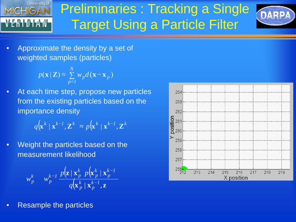
• Approximate the density by a set of weighted samples (particles)

• At each time step, propose new particles from the existing particles based on the importance density

• Weight the particles based on the measurement likelihood

• Resample the particles

∑=

−≈N

1pppwp )()|( xxZx δ

( ) ( )k1kkk1kk pq ZxxZxx ,|,| −− ≈

( ) ( )( )zxx

xxxz

,|

||1k

pkp

1kp

kp

kp1k

pkp

q

ppww −

−−∝

The Wrong Way to do Multitarget Tracking

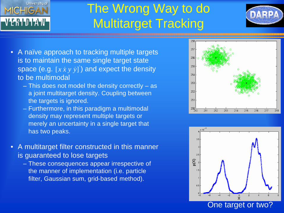
• A naïve approach to tracking multiple targets is to maintain the same single target state space (e.g. ) and expect the density to be multimodal

– This does not model the density correctly – as a joint multitarget density. Coupling between the targets is ignored.

– Furthermore, in this paradigm a multimodal density may represent multiple targets or merely an uncertainty in a single target that has two peaks.

• A multitarget filter constructed in this manner is guaranteed to lose targets

– These consequences appear irrespective of the manner of implementation (i.e. particle filter, Gaussian sum, grid-based method).

One target or two?

'] [ yyxx &&

The Wrong Way to do Multitarget Tracking

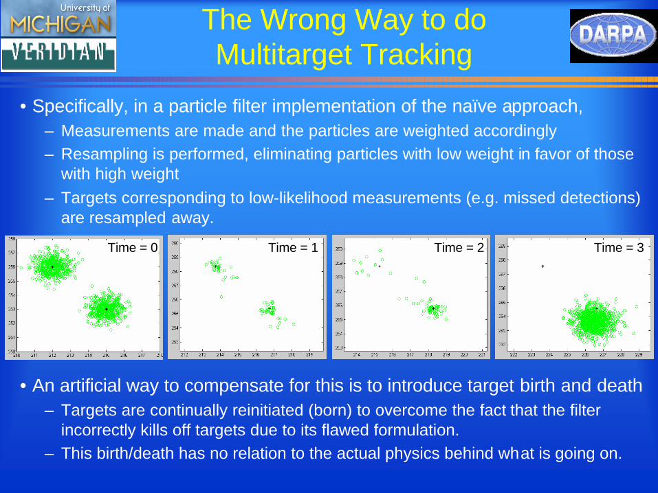
• Specifically, in a particle filter implementation of the naïve approach,– Measurements are made and the particles are weighted accordingly– Resampling is performed, eliminating particles with low weight in favor of those

with high weight– Targets corresponding to low-likelihood measurements (e.g. missed detections)

are resampled away.

• An artificial way to compensate for this is to introduce target birth and death– Targets are continually reinitiated (born) to overcome the fact that the filter

incorrectly kills off targets due to its flawed formulation.– This birth/death has no relation to the actual physics behind what is going on.

Time = 0 Time = 1 Time = 2 Time = 3

The Correct Formulation: The Joint MultitargetProbability Density (JMPD)

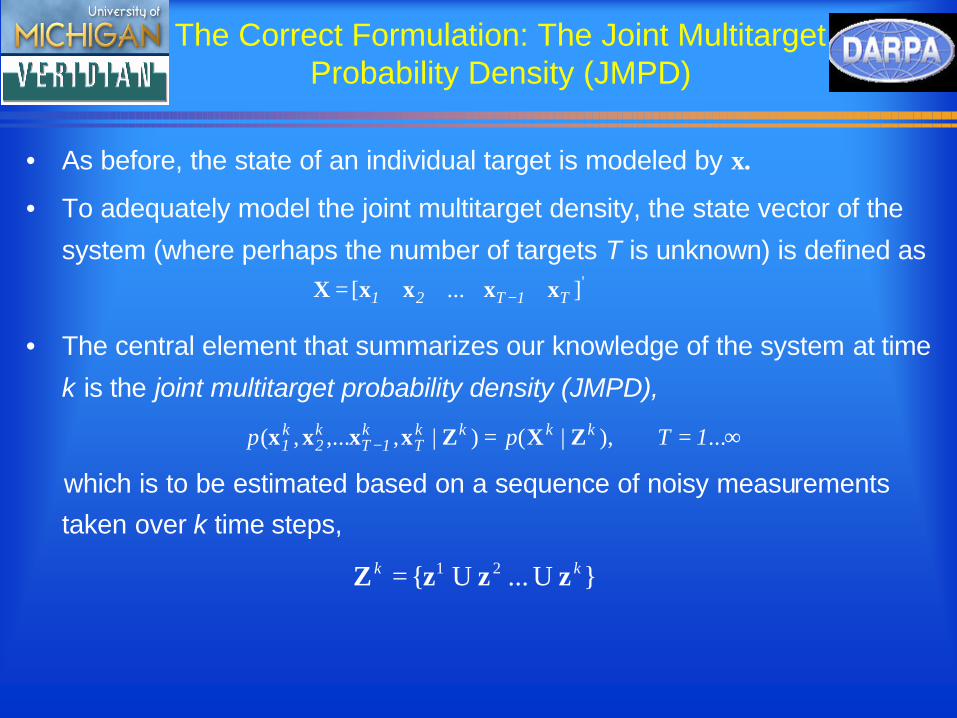
• As before, the state of an individual target is modeled by x.

• To adequately model the joint multitarget density, the state vector of the

system (where perhaps the number of targets T is unknown) is defined as

• The central element that summarizes our knowledge of the system at time

k is the joint multitarget probability density (JMPD),

which is to be estimated based on a sequence of noisy measurements

taken over k time steps,

} U... U{ 21 kk zzzZ =

']...[ T1T21 xxxxX −=

∞==− ... ),|()|,,...,( 1Tpp kkkkT

k1T

k2

k1 ZXZxxxx

The Joint MultitargetProbability Density (JMPD)

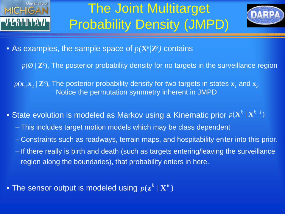
• As examples, the sample space of p(Xk|Zk) contains

• State evolution is modeled as Markov using a Kinematic prior– This includes target motion models which may be class dependent

– Constraints such as roadways, terrain maps, and hospitability enter into this prior.

– If there really is birth and death (such as targets entering/leaving the surveillance region along the boundaries), that probability enters in here.

• The sensor output is modeled using )|( kkp Xz

)|( 1kkp −XX

p(Ø | Zk), The posterior probability density for no targets in the surveillance region

p(x1,x2 | Zk), The posterior probability density for two targets in states x1 and x2Notice the permutation symmetry inherent in JMPD

The Joint MultitargetProbability Density (JMPD), cont’d

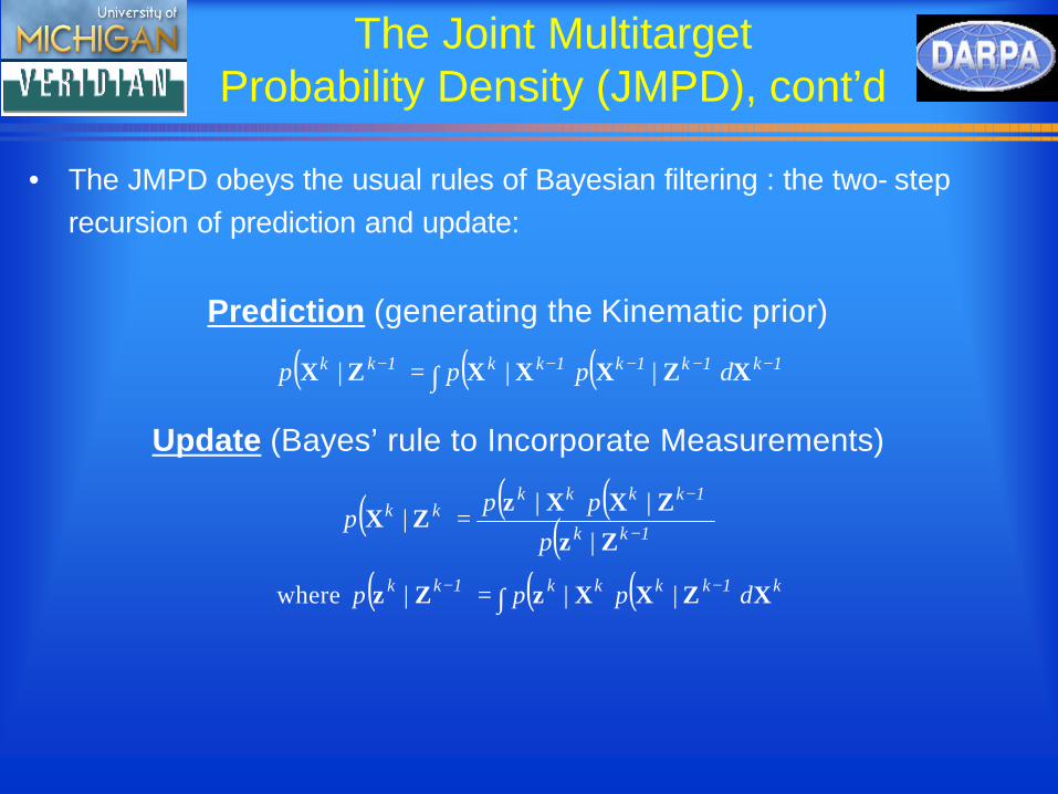
• The JMPD obeys the usual rules of Bayesian filtering : the two- step recursion of prediction and update:

( ) ( ) ( ) 1k1k1k1kk1kk dppp −−−−− ∫= XZXXXZX |||

( ) ( ) ( )( )1kk

1kkkkkk

p

ppp

−

−=

Zz

ZXXzZX

|

|||

( ) ( ) ( ) k1kkkk1kk dppp XZXXzZz −− ∫= ||| where

Prediction (generating the Kinematic prior)

Update (Bayes’ rule to Incorporate Measurements)

Particle Filter Implementation of JMPD

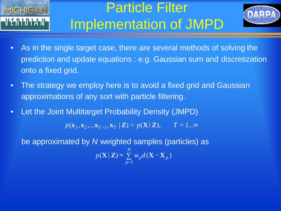
• As in the single target case, there are several methods of solving the prediction and update equations : e.g. Gaussian sum and discretizationonto a fixed grid.

• The strategy we employ here is to avoid a fixed grid and Gaussian approximations of any sort with particle filtering.

• Let the Joint Multitarget Probability Density (JMPD)

be approximated by N weighted samples (particles) as

∞==− ... ),|()|,,...,( 1Tpp T1T21 ZXZxxxx

∑=

−≈N

1pppwp )()|( XXZX δ

Particle Filter Implementation of JMPD

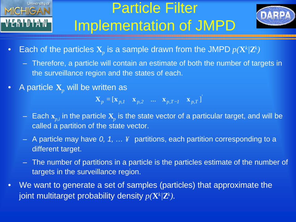
• Each of the particles Xp is a sample drawn from the JMPD p(Xk|Zk)

– Therefore, a particle will contain an estimate of both the number of targets in the surveillance region and the states of each.

• A particle Xp will be written as

– Each xp,i in the particle Xp is the state vector of a particular target, and will be called a partition of the state vector.

– A particle may have 0, 1, … ∞ partitions, each partition corresponding to a different target.

– The number of partitions in a particle is the particles estimate of the number of targets in the surveillance region.

• We want to generate a set of samples (particles) that approximate the joint multitarget probability density p(Xk|Zk).

',,,, ]...[ Tp1Tp2p1pp xxxxX −=

Design of Importance Density

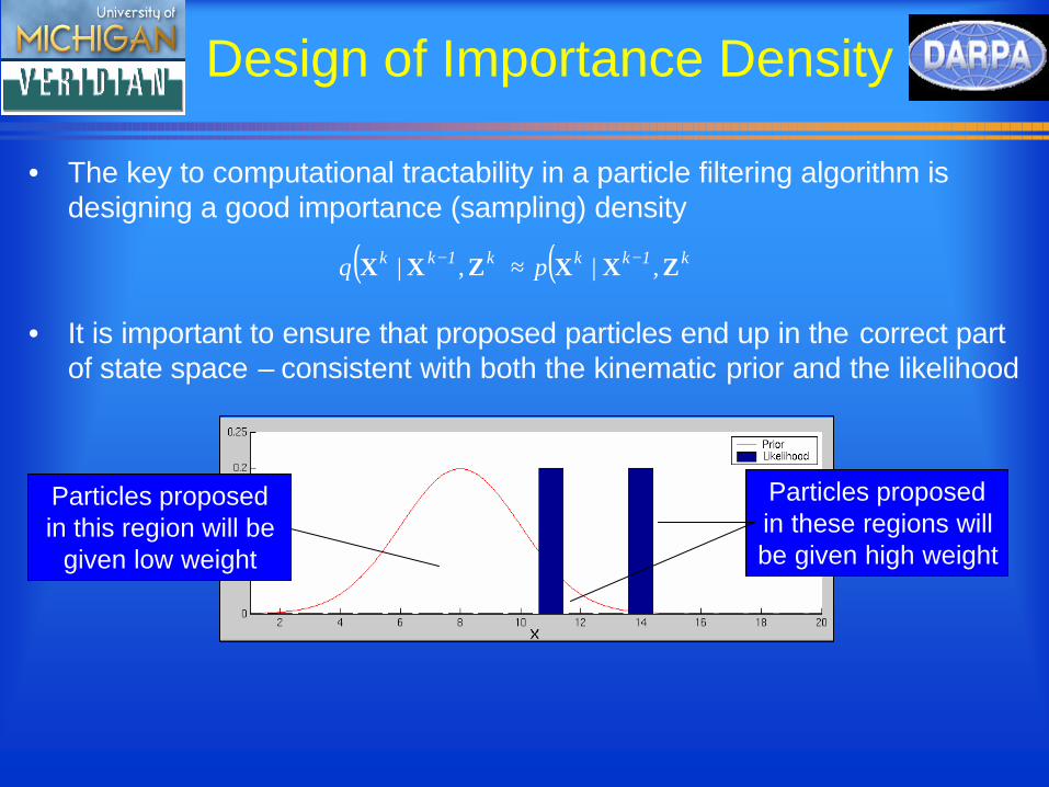
• The key to computational tractability in a particle filtering algorithm is designing a good importance (sampling) density

• It is important to ensure that proposed particles end up in the correct part of state space – consistent with both the kinematic prior and the likelihood

( ) ( )k1kkk1kk pq ZXXZXX ,|,| −− ≈

Particles proposed in this region will be

given low weight

Particles proposed in these regions will be given high weight

The Multitarget Proposal Density

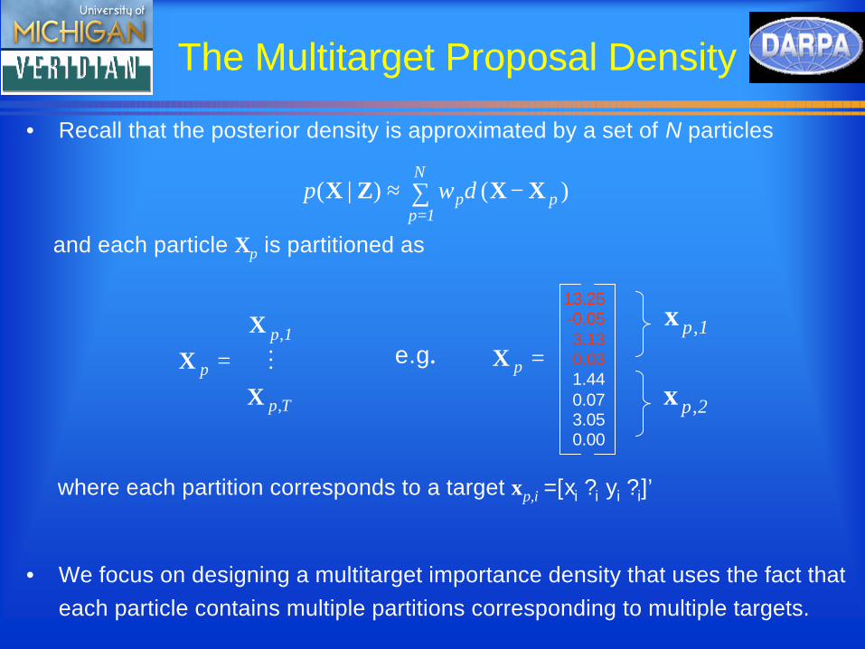
• Recall that the posterior density is approximated by a set of N particles

and each particle Xp is partitioned as

where each partition corresponds to a target xp,i =[xi ?i yi ?i]’

• We focus on designing a multitarget importance density that uses the fact that each particle contains multiple partitions corresponding to multiple targets.

∑=

−≈N

1pppwp )()|( XXZX δ

=

Tp

1p

p

,

,

X

XX M e.g. =pX

1p,x

2p,x

13.25-0.053.130.031.440.073.050.00

The Standard Importance Density: The Kinematic Prior

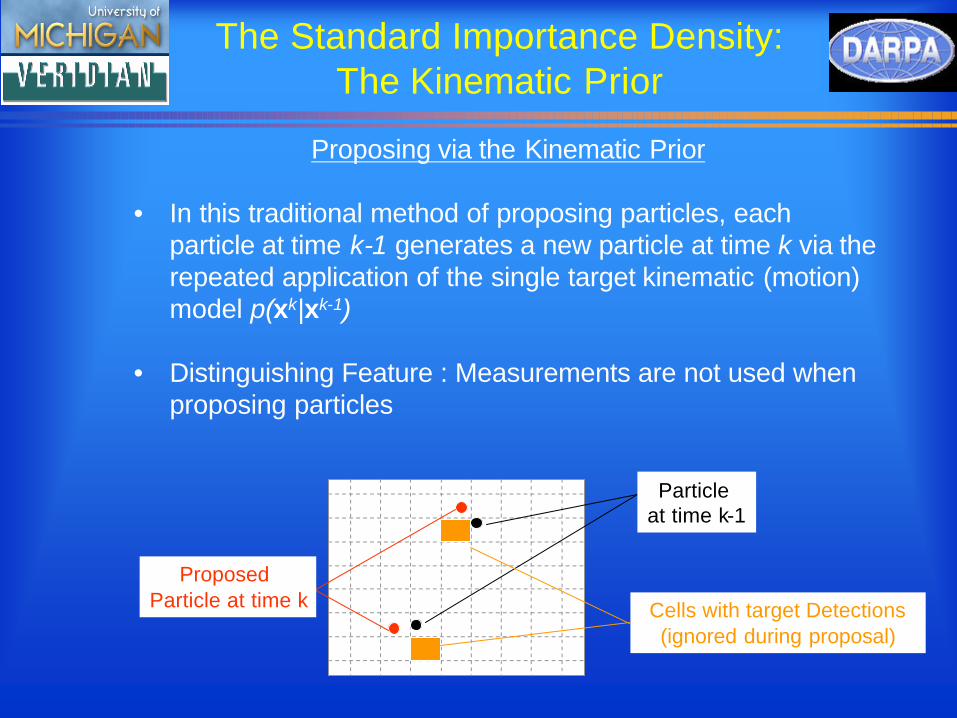
Proposing via the Kinematic Prior

• In this traditional method of proposing particles, each particle at time k-1 generates a new particle at time k via the repeated application of the single target kinematic (motion) model p(xk|xk-1)

• Distinguishing Feature : Measurements are not used when proposing particles

Particle at time k-1

Proposed Particle at time k Cells with target Detections

(ignored during proposal)

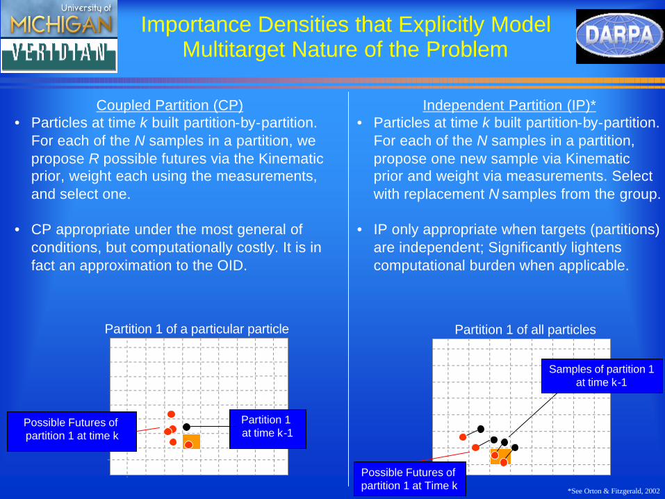
Importance Densities that Explicitly Model Multitarget Nature of the Problem

Coupled Partition (CP)• Particles at time k built partition-by-partition.

For each of the N samples in a partition, we propose R possible futures via the Kinematicprior, weight each using the measurements, and select one.

• CP appropriate under the most general of conditions, but computationally costly. It is in fact an approximation to the OID.

Independent Partition (IP)*• Particles at time k built partition-by-partition.

For each of the N samples in a partition, propose one new sample via Kinematicprior and weight via measurements. Select with replacement N samples from the group.

• IP only appropriate when targets (partitions) are independent; Significantly lightens computational burden when applicable.

Partition 1 at time k-1

Possible Futures of partition 1 at Time k

Samples of partition 1at time k-1

*See Orton & Fitzgerald, 2002

Possible Futures of partition 1 at time k

Partition 1 of a particular particle Partition 1 of all particles

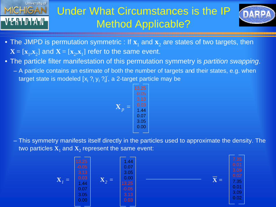
Under What Circumstances is the IP Method Applicable?

• The JMPD is permutation symmetric : If x1 and x2 are states of two targets, then X = [x1,x2] and X = [x2,x1] refer to the same event.

• The particle filter manifestation of this permutation symmetry is partition swapping.– A particle contains an estimate of both the number of targets and their states, e.g. when

target state is modeled [xi ? i yi ? i]’, a 2-target particle may be

– This symmetry manifests itself directly in the particles used to approximate the density. The two particles X1 and X2 represent the same event:

=X=1X =2X

13.25-0.053.130.031.440.073.050.00

1.440.073.050.00

13.25-0.053.130.03

7.350.013.090.027.350.013.090.02

=pX

13.25-0.053.130.031.440.073.050.00

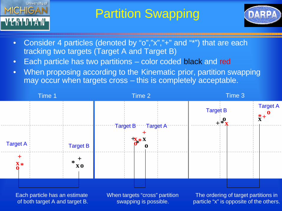
Partition Swapping

• Consider 4 particles (denoted by “o”,”x”,”+” and “*”) that are each tracking two targets (Target A and Target B)

• Each particle has two partitions – color coded black and red• When proposing according to the Kinematic prior, partition swapping

may occur when targets cross – this is completely acceptable.

Each particle has an estimate of both target A and target B.

The ordering of target partitions in particle “x” is opposite of the others.

When targets “cross” partition swapping is possible.

Time 1

o

o*+x o*

+x

Time 2

oo*+

xo*

+ x o

o*+

xo

*+x

Time 3

Target A Target B

Target ATarget B

Target ATarget B

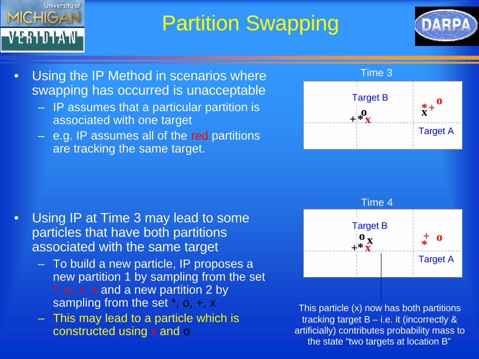
Partition Swapping

• Using the IP Method in scenarios where swapping has occurred is unacceptable– IP assumes that a particular partition is

associated with one target – e.g. IP assumes all of the red partitions

are tracking the same target.

• Using IP at Time 3 may lead to some particles that have both partitions associated with the same target– To build a new particle, IP proposes a

new partition 1 by sampling from the set *, o, +, x and a new partition 2 by sampling from the set *, o, +, x

– This may lead to a particle which is constructed using x and o

This particle (x) now has both partitions tracking target B – i.e. it (incorrectly &

artificially) contributes probability mass to the state “two targets at location B”

Time 3

Time 4

oo

*+x

o*+

x

Target A

Target B

o o*+

xo*+

x

Target A

Target B

Partition Swapping, cont’d

• The CP Method does not mix particles – lineage is maintained.– New particles will be proposed with the same ordering as particles

from the previous time step.– Permutation symmetry is respected and probability mass is not

artificially transferred to incorrect states.

• CP applicable in all scenarios.– Significantly less efficient then IP method– When IP appropriate, it should be used.

• IP applicable when targets are ‘well separated’ (acting independently) and the partitions are ordered identically.

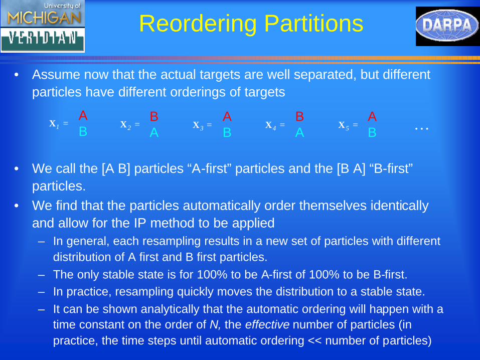
Reordering Partitions

• Assume now that the actual targets are well separated, but different particles have different orderings of targets

• We call the [A B] particles “A-first” particles and the [B A] “B-first” particles.

• We find that the particles automatically order themselves identically and allow for the IP method to be applied– In general, each resampling results in a new set of particles with different

distribution of A first and B first particles.– The only stable state is for 100% to be A-first of 100% to be B-first.– In practice, resampling quickly moves the distribution to a stable state.– It can be shown analytically that the automatic ordering will happen with a

time constant on the order of N, the effective number of particles (in practice, the time steps until automatic ordering << number of particles)

=1XAB

=2XBA

=3XAB

=4XBA

=5XAB …

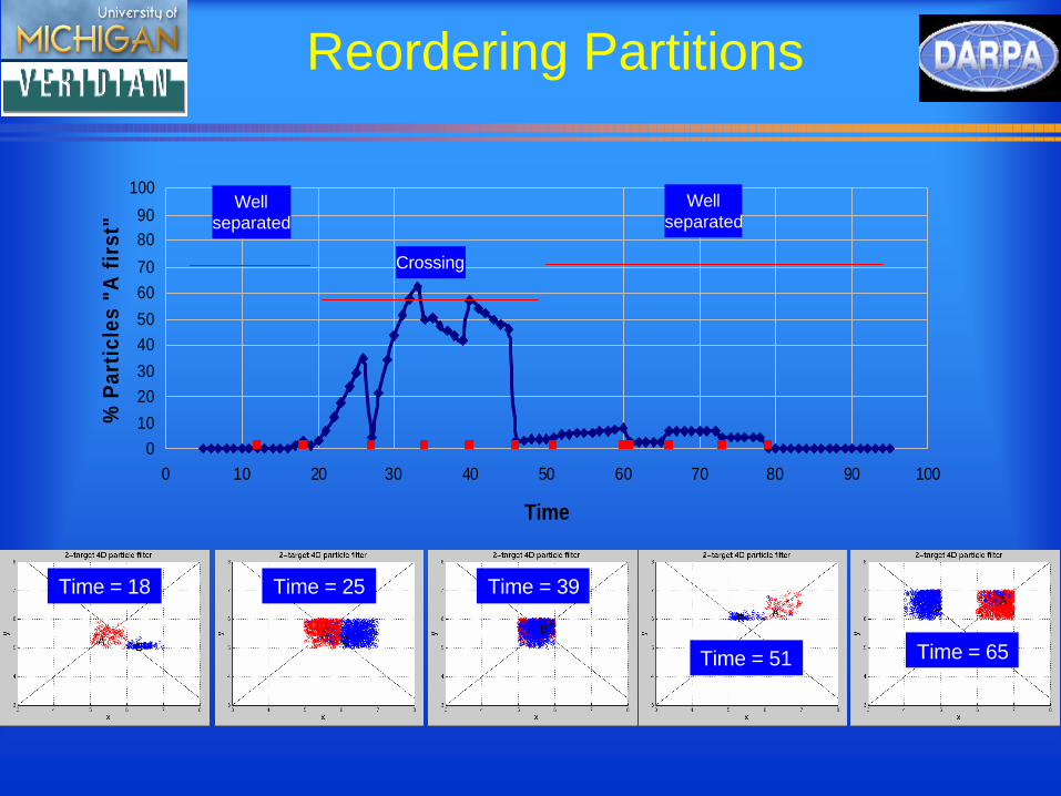
Reordering Partitions

Time = 18 Time = 25 Time = 39

Time = 51

010

2030

4050

6070

8090

100

0 10 20 30 40 50 60 70 80 90 100

Time

% P

arti

cles

"A

fir

st"

Wellseparated

Crossing

Wellseparated

Time = 65

Multitarget Proposal Densities

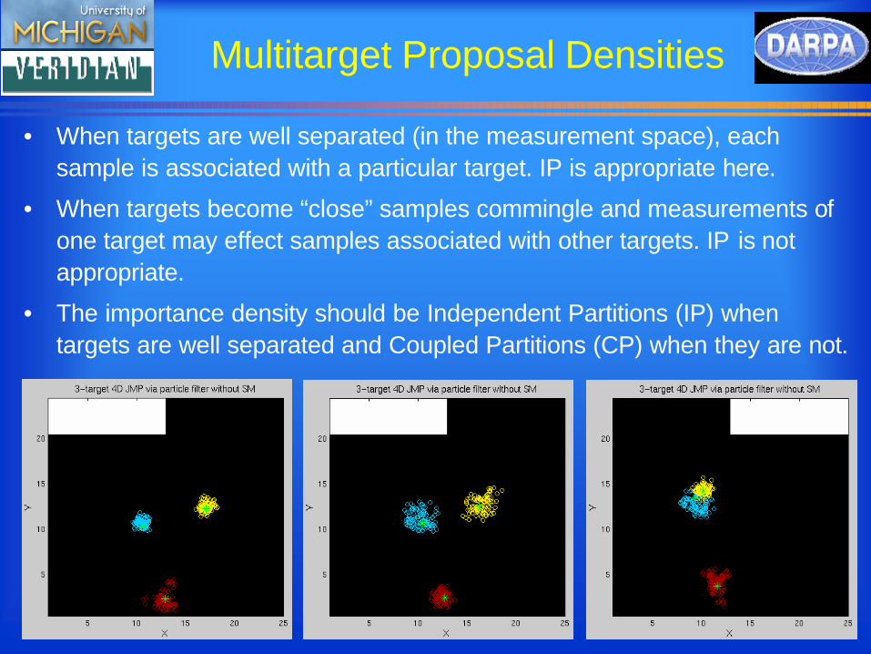
• When targets are well separated (in the measurement space), eachsample is associated with a particular target. IP is appropriate here.

• When targets become “close” samples commingle and measurements of one target may effect samples associated with other targets. IP is not appropriate.

• The importance density should be Independent Partitions (IP) when targets are well separated and Coupled Partitions (CP) when they are not.

Adaptive Proposal Method Switching

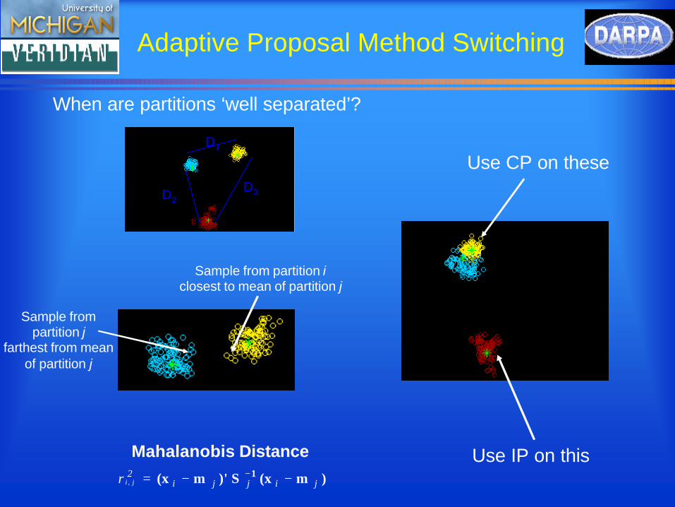
When are partitions ‘well separated’?

D1

D2D3

Sample from partition iclosest to mean of partition j

Sample from partition j

farthest from mean of partition j

Mahalanobis Distance

)m(xS)'m(x 1jijji

2jir −−= −

,

Use IP on this

Use CP on these

Multitarget Proposal Densities

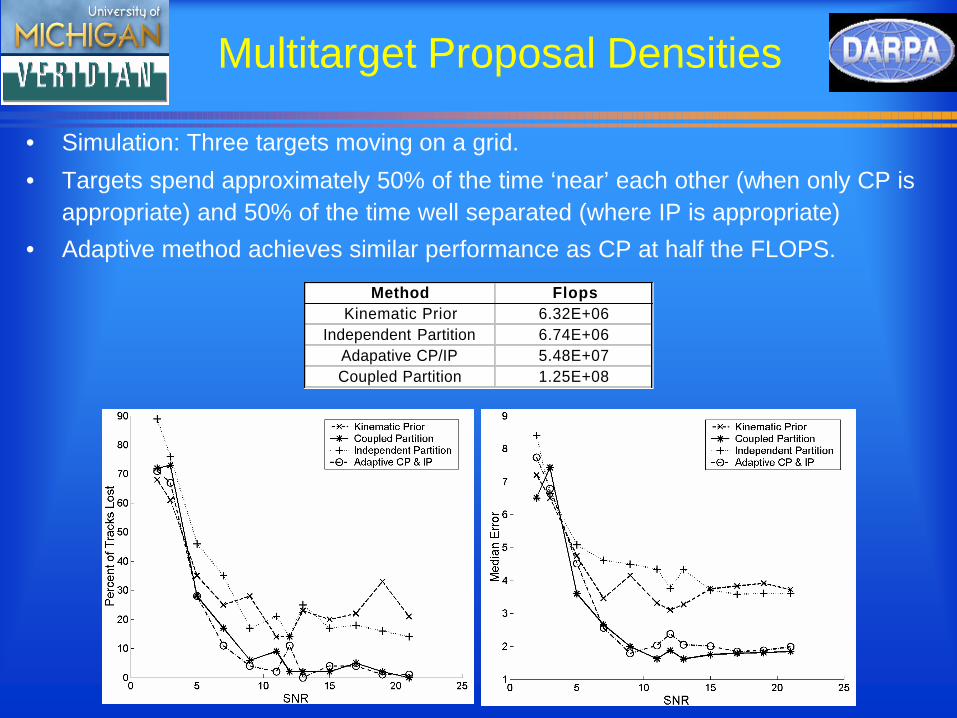
Method FlopsKinematic Prior 6.32E+06

Independent Partition 6.74E+06Adapative CP/IP 5.48E+07Coupled Partition 1.25E+08

• Simulation: Three targets moving on a grid.

• Targets spend approximately 50% of the time ‘near’ each other (when only CP is appropriate) and 50% of the time well separated (where IP is appropriate)

• Adaptive method achieves similar performance as CP at half the FLOPS.

How much Effort does the adaptive strategy save?

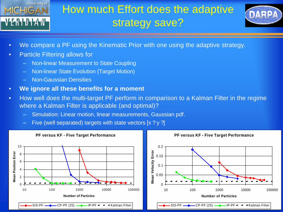
• We compare a PF using the Kinematic Prior with one using the adaptive strategy.

• Particle Filtering allows for– Non-linear Measurement to State Coupling– Non-linear State Evolution (Target Motion)– Non-Gaussian Densities

• We ignore all these benefits for a moment

• How well does the multi-target PF perform in comparison to a Kalman Filter in the regimewhere a Kalman Filter is applicable (and optimal)?

– Simulation: Linear motion, linear measurements, Gaussian pdf. – Five (well separated) targets with state vectors [x ? y ?]

PF versus KF - Five Target Performance

0

2

4

6

8

10

10 100 1000 10000 100000

Number of Particles

Mea

n P

osit

ion

Err

or

SIS-PF CP-PF (25) IP-PF Kalman Filter

PF versus KF - Five Target Performance

0

0.05

0.1

0.15

0.2

10 100 1000 10000 100000

Number of Particles

Mea

n V

eloc

ity

Err

or

SIS-PF CP-PF (25) IP-PF Kalman Filter

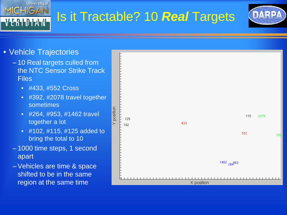
Is it Tractable? 10 Real Targets

• Vehicle Trajectories– 10 Real targets culled from

the NTC Sensor Strike Track Files

• #433, #552 Cross• #392, #2078 travel together

sometimes• #264, #953, #1462 travel

together a lot• #102, #115, #125 added to

bring the total to 10

– 1000 time steps, 1 second apart

– Vehicles are time & space shifted to be in the same region at the same time

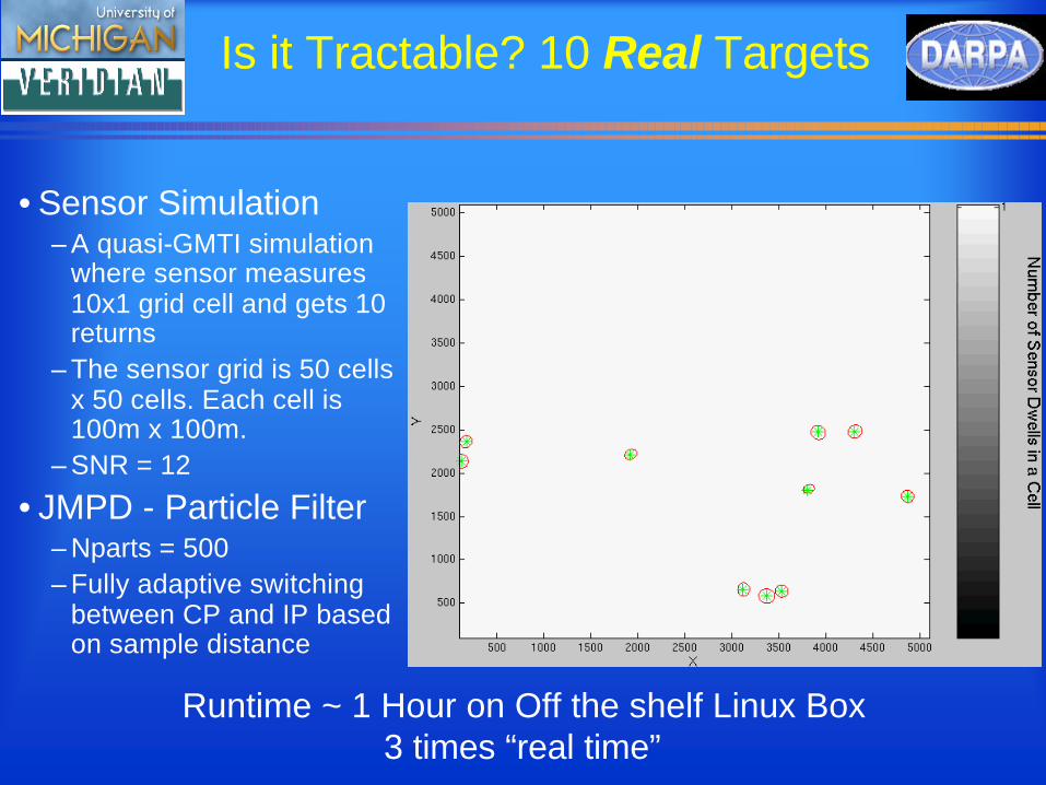
Is it Tractable? 10 Real Targets

• Sensor Simulation– A quasi-GMTI simulation

where sensor measures 10x1 grid cell and gets 10 returns

– The sensor grid is 50 cells x 50 cells. Each cell is 100m x 100m.

– SNR = 12

• JMPD - Particle Filter– Nparts = 500– Fully adaptive switching

between CP and IP based on sample distance

Runtime ~ 1 Hour on Off the shelf Linux Box3 times “real time”

Conclusion

• We’ve presented a method of tracking multiple targets based on recursive estimation of their Joint Multitarget Probability Density (JMPD).

• Computational tractability is provided by Particle Filter-based implementation.

– Adaptive sampling schemes exploit multitarget nature of the problem.

– Permutation symmetry manifests itself as partition swapping

• Natural framework to do sensor management where the JMPD is used to compute the area of maximal expected information gain.

• Backup slides: Information based sensor management using the particle filter implementation of JMPD.

Information Based Sensor Management

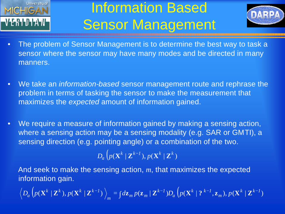
• The problem of Sensor Management is to determine the best way to task a sensor where the sensor may have many modes and be directed in many manners.

• We take an information-based sensor management route and rephrase the problem in terms of tasking the sensor to make the measurement that maximizes the expected amount of information gained.

• We require a measure of information gained by making a sensing action, where a sensing action may be a sensing modality (e.g. SAR or GMTI), a sensing direction (e.g. pointing angle) or a combination of the two.

And seek to make the sensing action, m, that maximizes the expected information gain.

( ))|(),|( kk1kk ppD ZXZX −α

( ) ( ))|(),,|()|()|(),|( 1kkm

1kk1kmmm

1kkkk ppDpdppD −−−− ∫= ZXz?XZzzZXZX αα

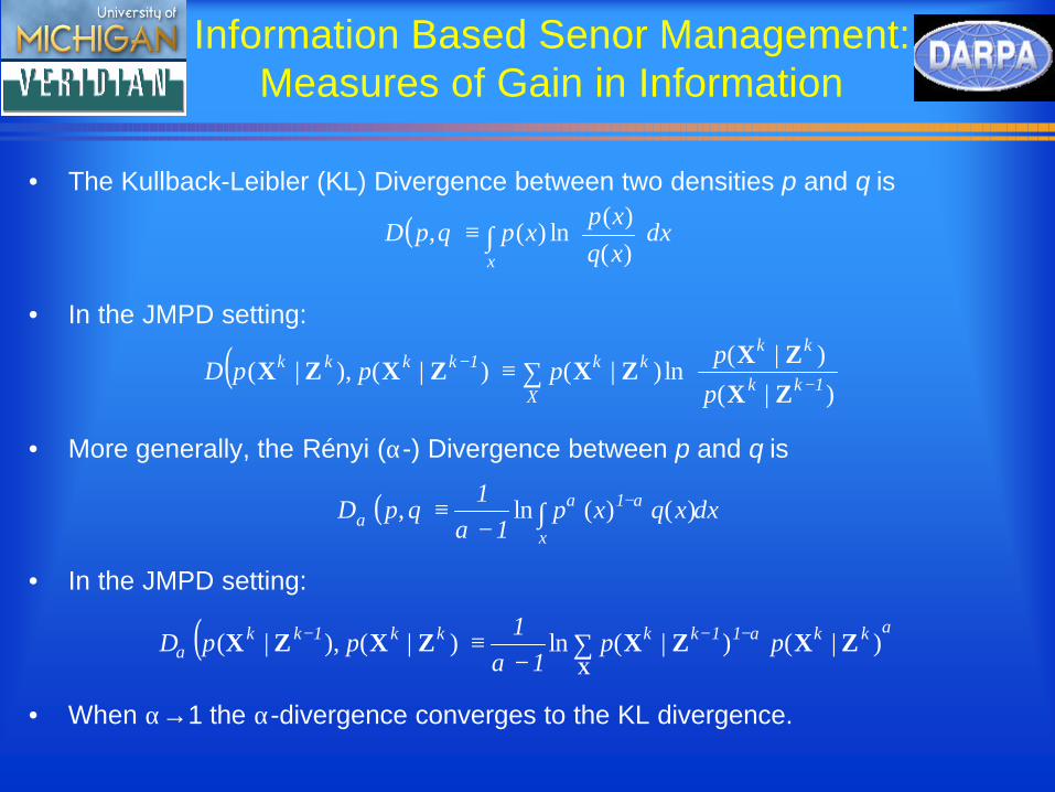
Information Based Senor Management: Measures of Gain in Information

• The Kullback-Leibler (KL) Divergence between two densities p and q is

• In the JMPD setting:

• More generally, the Rényi (α-) Divergence between p and q is

• In the JMPD setting:

• When α→1 the α-divergence converges to the KL divergence.

( ) ∑

≡ −

−

X1kk

kkkk1kkkk

p

ppppD

)|(

)|(ln)|()|(),|(

ZX

ZXZXZXZX

( ) dxxqxp

xpqpDx∫

≡

)()(

ln)(,

( ) dxxqxp1

1qpD

x

1∫ −

−≡ )()(ln, αα

α α

( ) ααα α

∑ −−−

−≡

XZXZXZXZX )|()|(ln)|(),|( kk11kkkk1kk pp

11

ppD

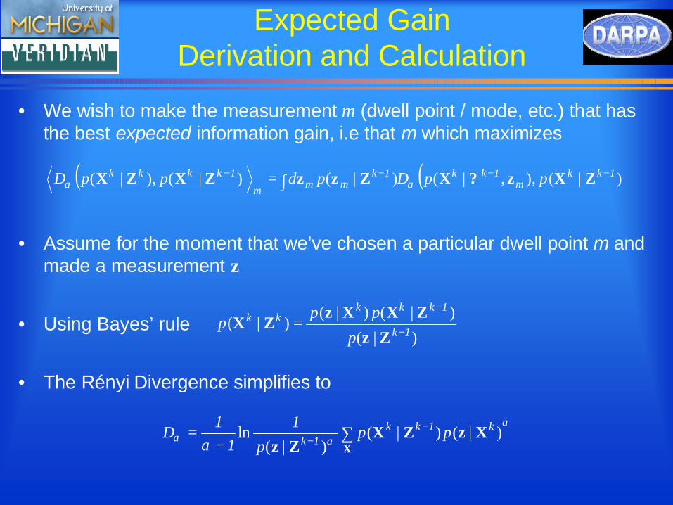
Expected Gain Derivation and Calculation

• We wish to make the measurement m (dwell point / mode, etc.) that has the best expected information gain, i.e that m which maximizes

• Assume for the moment that we’ve chosen a particular dwell point m and made a measurement z

• Using Bayes’ rule

• The Rényi Divergence simplifies to

( ) ( ))|(),,|()|()|(),|( 1kkm

1kk1kmmm

1kkkk ppDpdppD −−−− ∫= ZXz?XZzzZXZX αα

)|(

)|()|()|(

1k

1kkkkk

p

ppp

−

−=

Zz

ZXXzZX

α

αα α∑ −

−−=

XXzZX

Zz)|()|(

)|(ln k1kk

1kpp

p1

11

D

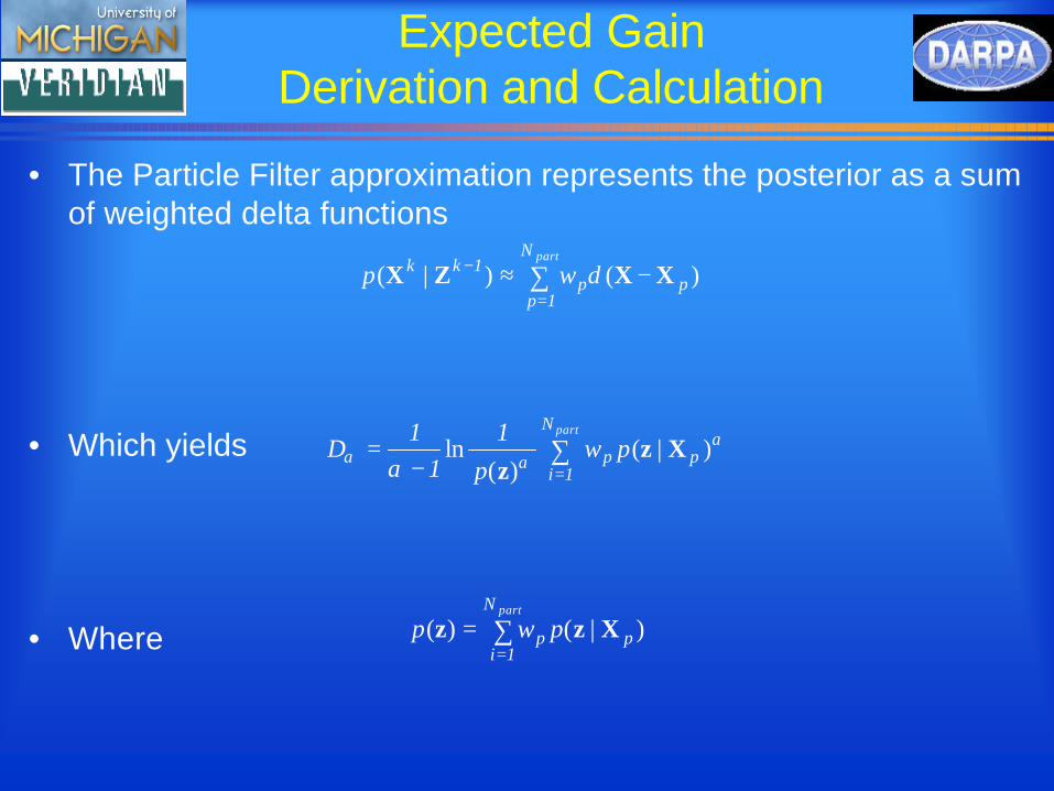
Expected Gain Derivation and Calculation

• The Particle Filter approximation represents the posterior as a sum of weighted delta functions

• Which yields

• Where

∑=−

=partN

1ipp pw

p1

11

D ααα α

)|()(

ln Xzz

∑=

− −≈partN

1ppp

1kk wp )()|( XXZX δ

∑=

=partN

1ipp pwp )|()( Xzz

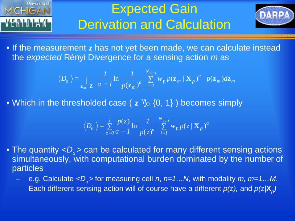
Expected Gain Derivation and Calculation

• If the measurement z has not yet been made, we can calculate instead the expected Rényi Divergence for a sensing action m as

• Which in the thresholded case ( zg {0, 1} ) becomes simply

• The quantity <Dα> can be calculated for many different sensing actions simultaneously, with computational burden dominated by the number of particles– e.g. Calculate <Dα> for measuring cell n, n=1…N, with modality m, m=1…M.– Each different sensing action will of course have a different p(z), and p(z|Xp)

mm

N

1ipmp

m

dppwp

11

1D

m

part

zzXzzZz

)()|()(

ln∫ ∑∈ =

−= α

αα α

∑ ∑= =−

=1

0z

N

1ipp

part

zpwzp1

1zp

D ααα α

)|()(

ln)(

X

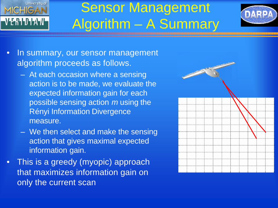
Sensor Management Algorithm – A Summary

• In summary, our sensor management algorithm proceeds as follows. – At each occasion where a sensing

action is to be made, we evaluate the expected information gain for each possible sensing action m using the Rényi Information Divergence measure.

– We then select and make the sensing action that gives maximal expected information gain.

• This is a greedy (myopic) approach that maximizes information gain on only the current scan

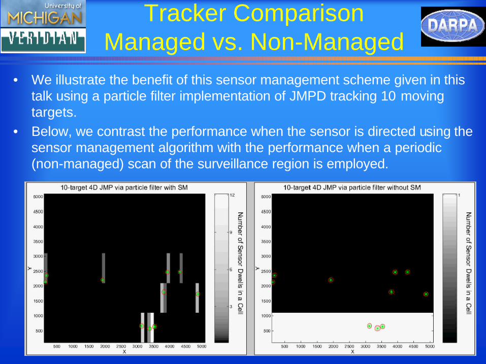
Tracker ComparisonManaged vs. Non-Managed

• We illustrate the benefit of this sensor management scheme given in this talk using a particle filter implementation of JMPD tracking 10 moving targets.

• Below, we contrast the performance when the sensor is directed using the sensor management algorithm with the performance when a periodic(non-managed) scan of the surveillance region is employed.

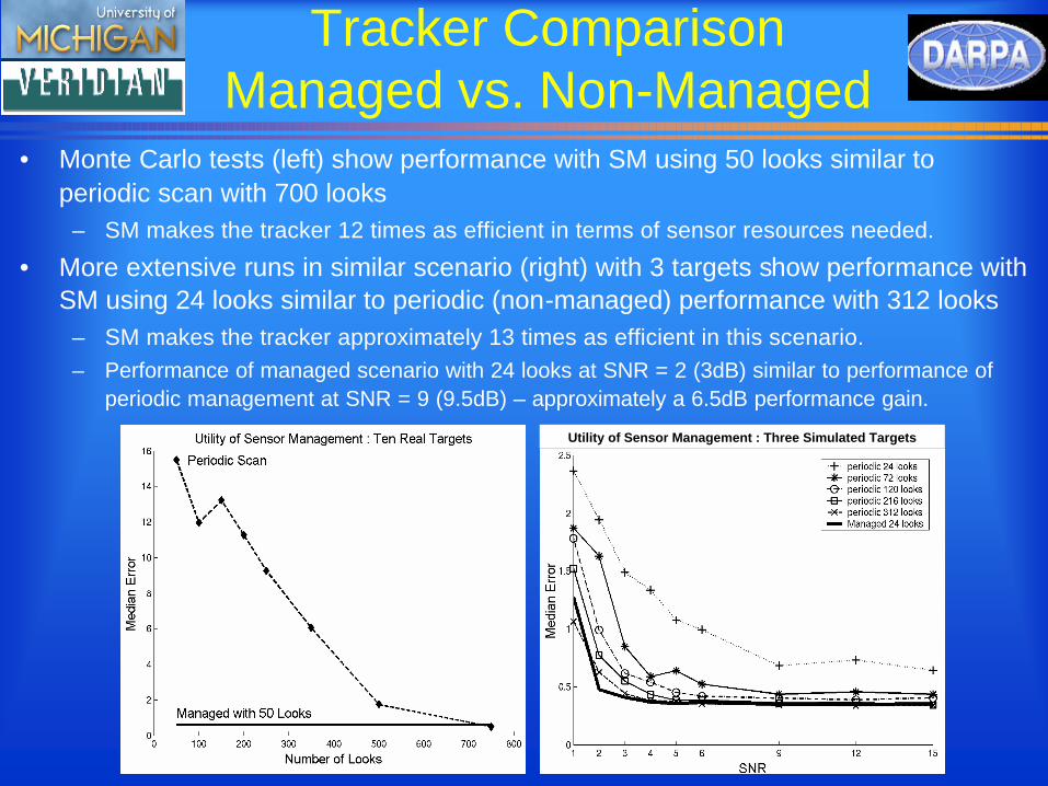
Tracker ComparisonManaged vs. Non-Managed

• Monte Carlo tests (left) show performance with SM using 50 looks similar to periodic scan with 700 looks

– SM makes the tracker 12 times as efficient in terms of sensor resources needed.

• More extensive runs in similar scenario (right) with 3 targets show performance with SM using 24 looks similar to periodic (non-managed) performance with 312 looks

– SM makes the tracker approximately 13 times as efficient in this scenario.– Performance of managed scenario with 24 looks at SNR = 2 (3dB) similar to performance of

periodic management at SNR = 9 (9.5dB) – approximately a 6.5dB performance gain.

Utility of Sensor Management : Three Simulated Targets

The Information Based Method Automatically Optimizes Across Modes

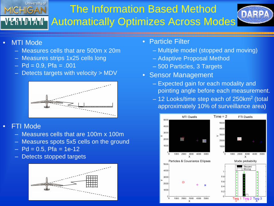
• MTI Mode– Measures cells that are 500m x 20m– Measures strips 1x25 cells long– Pd = 0.9, Pfa = .001– Detects targets with velocity > MDV

• FTI Mode– Measures cells that are 100m x 100m– Measures spots 5x5 cells on the ground– Pd = 0.5, Pfa = 1e-12– Detects stopped targets

• Particle Filter– Multiple model (stopped and moving)– Adaptive Proposal Method– 500 Particles, 3 Targets

• Sensor Management– Expected gain for each modality and

pointing angle before each measurement.– 12 Looks/time step each of 250km2 (total

approximately 10% of surveillance area)

Optimizing Collection Strategy Across Modes

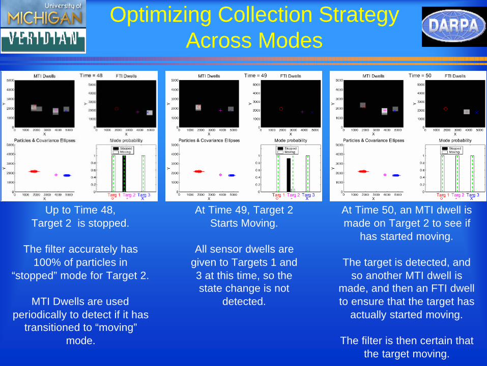
Up to Time 48, Target 2 is stopped.

The filter accurately has 100% of particles in

“stopped” mode for Target 2.

MTI Dwells are used periodically to detect if it has

transitioned to “moving” mode.

At Time 49, Target 2 Starts Moving.

All sensor dwells are given to Targets 1 and 3 at this time, so the state change is not

detected.

At Time 50, an MTI dwell is made on Target 2 to see if

has started moving.

The target is detected, and so another MTI dwell is

made, and then an FTI dwell to ensure that the target has

actually started moving.

The filter is then certain that the target moving.

The Information Based Method Automatically Optimizes Across Modes

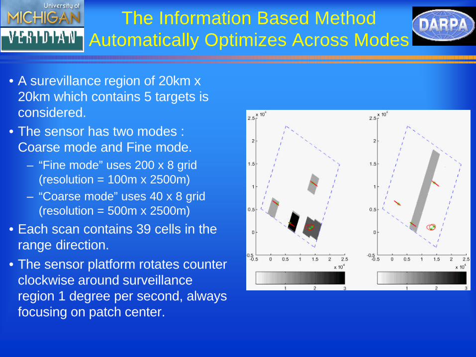
• A surevillance region of 20km x 20km which contains 5 targets is considered.

• The sensor has two modes : Coarse mode and Fine mode.

– “Fine mode” uses 200 x 8 grid (resolution = 100m x 2500m)

– “Coarse mode” uses 40 x 8 grid (resolution = 500m x 2500m)

• Each scan contains 39 cells in the range direction.

• The sensor platform rotates counter clockwise around surveillance region 1 degree per second, always focusing on patch center.

Conclusions and Future Work

• We’ve presented a method of tracking multiple targets and sensor management based on recursive estimation of the Joint Multitarget Probability Density (JMPD).

– Computational tractability is provided by Particle Filter-based implementation with adaptive sampling schemes that exploit multitarget nature of the problem.

• We have demonstrated a method of sensor management (SM) which uses the JMPD and tasks the sensor to make measurements that yield the maximum expected information gain.

– In the application of tracking multiple moving ground targets, SM of this type is able to use the sensor more than 10 times as efficiently as a simple periodic scan.

– The method automatically captures the tradeoff between sensor modalities (e.g. fine resolution mode vs. coarse resolution mode, GMTI mode vs. SAR mode) without any ad hoc adjustments.

• The SM algorithm presented is myopic (greedy).

– Sensor platform motion (not modeled here) makes it important to plan ahead and choose optimal measurement sequences rather than just individual measurements

– Future work includes extending these principles to non-myopic sensor management, perhaps using a MDP formulation and Monte Carlo or rollout type solutions.