Transfer Learning with intelligent training data selection ... · we pick the training data that would provide the most amount of information through image entropy. We show that through

Date of publication xxxx 00, 0000, date of current version xxxx 00, 0000.

Digital Object Identifier 10.1109/ACCESS.2017.DOI

Transfer Learning with intelligenttraining data selection for prediction ofAlzheimer’s DiseaseNAIMUL MEFRAZ KHAN1, (Member, IEEE), NABILA ABRAHAM1, (Member, IEEE), MARCIAHON11Ryerson University, Toronto, ON M5B2K3 Canada.

Corresponding author: Naimul Mefraz Khan (e-mail: [email protected]).

ABSTRACT Detection of Alzheimer’s Disease (AD) from neuroimaging data such as MRI throughmachine learning has been a subject of intense research in recent years. Recent success of deep learning incomputer vision has progressed such research further. However, common limitations with such algorithmsare reliance on a large number of training images, and requirement of careful optimization of the architectureof deep networks. In this paper, we attempt solving these issues with transfer learning, where the state-of-the-art VGG architecture is initialized with pre-trained weights from large benchmark datasets consisting ofnatural images. The network is then fine-tuned with layer-wise tuning, where only a pre-defined group oflayers are trained on MRI images. To shrink the training data size, we employ image entropy to select themost informative slices. Through experimentation on the ADNI dataset, we show that with training size of10 to 20 times smaller than the other contemporary methods, we reach state-of-the-art performance in ADvs. NC, AD vs. MCI, and MCI vs. NC classification problems, with a 4% and a 7% increase in accuracyover the state-of-the-art for AD vs. MCI and MCI vs. NC, respectively. We also provide detailed analysisof the effect of the intelligent training data selection method, changing the training size, and changing thenumber of layers to be fine-tuned. Finally, we provide Class Activation Maps (CAM) that demonstrate howthe proposed model focuses on discriminative image regions that are neuropathologically relevant, and canhelp the healthcare practitioner in interpreting the model’s decision making process.

INDEX TERMS Deep Learning, Transfer Learning, Convolutional Neural Network, Alzheimer’s

I. INTRODUCTION

ALZHEIMER’S Disease (AD) is a neurodegenerativedisease causing dementia in elderly population. It is

predicted that one out of every 85 people will be affectedby AD by 2050 [1]. Early diagnosis of AD can be achievedthrough automated analysis of MRI images with machinelearning. It has been shown recently that in some cases,machine learning algorithms can predict AD better thanclinicians [2], making it an important field of research forcomputer-aided diagnosis.

While statistical machine learning methods such as Sup-port Vector Machine (SVM) [3] have shown early success inautomated detection of AD, recently deep learning methodssuch as Convolutional Neural Networks (CNN) and sparseautoencoders have outperformed statistical methods. How-ever, the existing deep learning methods train deep architec-tures from scratch, which has a few limitations [4], [5]: 1)

properly training a deep learning network requires a hugeamount of annotated training data, which can be a problemespecially for the medical imaging field where physician-annotated data can be expensive, and protected from cross-institutional use due to ethical and privacy reasons; 2) train-ing a deep network with large number of images requirehuge amount of computational resources; and 3) deep net-work training requires careful and tedious tuning of manyparameters, sub-optimal tuning of which can result in over-fitting/underfitting, and, in turns, result in poor performance.

An attractive alternative to training from scratch is fine-tuning a deep network (especially CNN) through transferlearning [6]. In popular computer vision domains such as ob-ject recognition, trained CNNs are carefully built using large-scale datasets such as ImageNet [7]. The idea of transferlearning is to train an already-trained (pre-trained) CNN tolearn new image representations using a smaller dataset from

VOLUME 4, 2016 1

arX

iv:1

906.

0116

0v1

[cs

.CV

] 4

Jun

201

9

N.M. Khan et al.: Transfer Learning with intelligent training data selection for prediction of Alzheimer’s Disease

a different problem. It has been shown that CNNs are verygood feature learners [8], and can generalize image featuresgiven a large training set. If we always train a network fromscratch, this attractive property of CNN is not being utilized,especially given the popularity of CNN and the existence ofproven architectures and datasets.

In this paper, we investigate how transfer learning canbe applied for improved diagnosis of AD. The key moti-vation behind employing transfer learning is to reduce thedependency on a large training set. To achieve state-of-the-art performance while using a smaller training set, we alsoemploy an intelligent filtering approach to reduce the trainingset. The key contributions of our method can be summarizedas follows:

• We employ layer-wise transfer learning on a state-of-the-art CNN architecture, where group of top layers inthe CNN are gradually trained while keeping the lower-level layers frozen. Employing transfer learning in thismanner is expected to produce different results, as themore levels we train, the further we are moving awayfrom a pre-trained network. We observe that to achievethe best possible result, only a few top layers are neededto be re-trained, which is very encouraging for reductionof required training time.

• Since our target is to test the robustness of transfer learn-ing on a small training set, merely choosing trainingdata at random may not provide us with a dataset rep-resenting enough structural variations in MRI. Instead,we pick the training data that would provide the mostamount of information through image entropy.

We show that through intelligent training data selec-tion and transfer learning, we can achieve state-of-the-artclassification results for all three classification scenariosin Alzheimer’s prediction, namely, AD vs Normal Control(NC), Mild Cognitive Impairment (MCI) vs. AD, and MCIvs. NC; while utilizing training data size of 10 to 20 timessmaller than the contemporary methods.

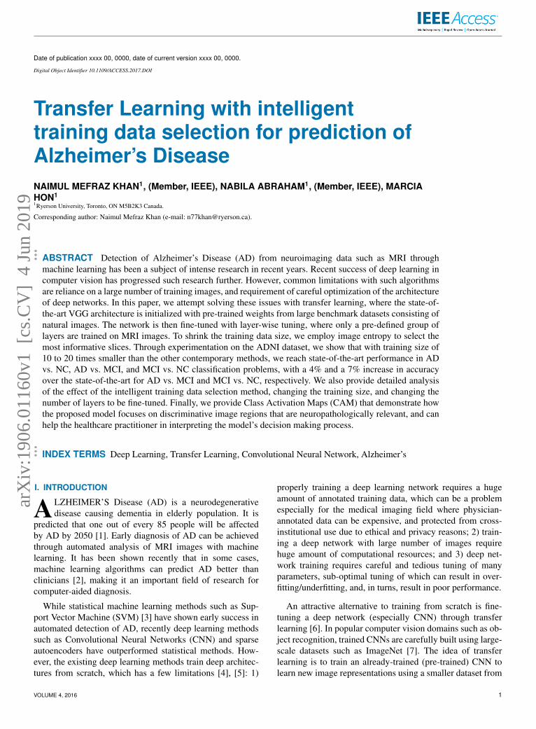
Figure 1 shows a high-level flow diagram of the proposedframework. As can be seen, information is extracted fromlabeled training data (MRI slices) in the training phase,through which the model learns which discriminative regions(shown in red) of an image it should focus on to distinguishdifferent cases. After deployment, individual slices can becategorized into different cases (AD, MCI, or NC) by uti-lizing the previously learned distinctive representation.

II. RELATED WORKSClassical machine learning methods such as SVM and feed-forward neural networks have been applied successfully todiagnose AD from structural MRI images [3], [9]. One suchrecent method is [9], where a dual-tree complex wavelettransform is used to extract features, and a feed-forward neu-ral network is used to classify images. Elaborate discussionand comparative results with other popular classical methodscan also be found in [9].

Training

AD MCI NC

Labeled data

Proposed

Model

Learned

Representation

Learned

Representation

Proposed

Model Query Image

Decision

Deployment

FIGURE 1: The end-to-end framework of the proposed sys-tem

Recently, deep learning methods have outperformed clas-sical methods by a large margin. As such, many such methodshave been proposed for diagnosis of AD. A combination ofpatches extracted from an autoencoder followed by convo-lutional layers for feature extraction were used in [10]. Themethod was further improved by using 3D convolution in[11]. Stacked autoencoders followed by a softmax layer forclassification was used in [12]. Popular CNN architecturessuch as LeNet and the first Inception model were used in [13].A new 3D-CNN architecture to extract voxel features wasused in [14]. Some of the proposed methods also leverageinformation from other imaging modalities (e.g. PET) andnon-imaging data from cognitive experiments [15]. Somerecent methods utilize resting state functional MRI datato model the functional connectivity network, followed byfeature extraction and classification from the modeled brainconnectome [16], [17]. These computational models are par-ticularly useful for MCI diagnosis.

Most of these methods provide experimental results onimages from the Alzheimer’s Disease Neuroimaging Ini-tiative (ADNI) database [18], the benchmark database forsolving the problem. The results are usually reported in theform of binary classification problems, where results arepublished showing performance of three binary classifiers:AD vs Normal Control (NC), Mild Cognitive Impairment(MCI) vs. AD, and MCI vs. NC. While these deep learn-ing methods provide decent accuracy results, none of thesemethods address the issue of dependence on a large numberof training samples. For a computer-aided diagnosis systemto be practical and usable in a real clinical setting, the depen-

2 VOLUME 4, 2016


dence on a large training set is a problem, since physician-annotated data may not be available/expensive to acquire.Our method addresses this research gap. As we show in theexperiments, our intelligent training data selection and use oftransfer learning provides noticeable improvement over thestate-of-the-art in terms of accuracy while utilizing a trainingsize of 10 to 20 times smaller than the methods mentionedabove.

A. CONVOLUTIONAL NEURAL NETWORKS ANDTRANSFER LEARNINGThe core of Convolutional Neural Networks (CNN) are lay-ers which can extract local features (e.g. edges) across an in-put image through convolution. Each node in a convolutionallayer is connected to a small subset of spatially connectedneurons. To search for the same local feature throughout theinput image, the connection weights are shared between thenodes in the convolutional layers. Each set of shared weightsis called a convolution kernel. To reduce computational com-plexity, each sequence of convolution layers is followed bya pooling layer [5]. The max pooling layer is the most com-mon, which reduces the size of feature maps by selecting themaximum feature response in local neighborhoods. CNNstypically consist of several pairs of convolutional and poolinglayers, followed by a number of consecutive fully connectedlayers, and finally a softmax layer, or regression layer, togenerate the output labels.

CNNs are trained with backpropagation [19], where un-known weights for each layer are iteratively updated tominimize a specific cost function. Typically, the weightsare initialized with a random set of values. However, thelarge number of weights typically associated with a CNNrequires a large number of training samples so that theiterative backpropagation algorithm can converge properly.Having a limited number of training samples can result in thealgorithm being stuck at a local minima, which will resultin suboptimal classification performance. An alternative torandomized weight initialization is transfer learning or fine-tuning, where the weights of the CNN are copied from anetwork that has already been trained on a larger dataset.

Transfer learning or fine-tuning has also been explored inmedical imaging. [5] provides an in-depth discussion andcomparative results of training from scratch vs fine-tuningon some medical applications. They show that in most cases,fine-tuning outperforms training from scratch. Fine-tunedCNNs have been used to localize planes in ultrasound im-ages [20], classify interstitial lung diseases [21], and retrievemissing or noisy plane views in cardiac imaging [22]. In [23],a methodology for classifying multimodal medical imagingdata is presented using an ensemble of CNNs and transferlearning. All these methods prove that employing transferlearning in the medical imaging domain has tremendousvalue, and has the potential to achieve high accuracy in ADdetection with smaller training dataset when compared totraining from scratch.

III. METHODOLOGYA. NETWORK ARCHITECTUREDue to the popularity of CNN, there are many establishedarchitectures that have been carefully constructed by re-searchers over the last few years to solve visual classificationproblems. The benchmark for evaluating the best architec-tures has been the ImageNet Large Scale Visual RecognitionChallenge (ILSVRC), where the participants are given thetask to classify images of 1000 different objects [7]. Thethorough evaluation nature of the ILSVRC challenge ensuresthat the architectures that are ranked top in terms of perfor-mance are very robust and well tested. The philosophy oftransfer learning is to utilize well designed architectures fornew tasks. Therefore, we investigated the recent winners ofthe ILSVRC challenge to identify an architecture that will besuitable for Alzheimer’s diagnosis.

We closely follow the VGG architecture [24] proposed bythe Oxford Visual Geometry Group which won the ILSVRC2014 challenge. The reason behind following the VGG archi-tecture is not only the high accuracy, but also the efficiency,and more importantly, adaptability to other image classifi-cation problems than ImageNet [24]. The architecture hasrecently been shown to be successful in computer-aided di-agnosis problems as well [25]. The key idea behind the archi-tecture is to increase the depth of the network by adding moreconvolutional layers while keeping other network parametersfixed. To manage the number of trainable parameters, theconvolution filter size is kept very small (3X3) throughoutall layers.

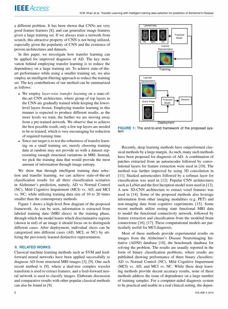
The architecture of our model can be seen in Figure 2.This architecture closely follows the VGG-19 architecture asproposed in the original work [24] with some changes in thefinal classification layer to adapt to our problem. An inputimage is passed through a stack of convolutional layers withkernel size of 3X3. We employed 16 convolutional layers[24] with 5 blocks:

1) Block 1: 2 layers with 3X3 convolution filters, 64channels.





16 convolutional layers correspond to the deepest archi-tecture in the VGG family, the VGG-19 architecture [24].Since network depth is the key property that makes VGG sorobust, we followed the deepest architecture. The filter size isalways fixed at 3X3, the smallest size to capture the notion ofleft/right, up/down, center. The width of the layers (numberof channels) increase as we progress through the network tolater layers. The increase in number of channels in later layersis important since the later layers capture more complex

VOLUME 4, 2016 3


Conv

(64)

Conv

(64)

poolin

g

Conv

(128)

Conv

(128)

Conv

(256)

Conv

(256)

Conv

(256)

Conv

(256)

Conv

(512)

Conv

(512)

Conv

(512)

Conv

(512)

Conv

(512)

Conv

(512)

Conv

(512)

Conv

(512)

poolin

g

poolin

gp

oolin

gp

oolin

g

FC

(256)

FC

(1)

Convolution

and

Pooling

Layers

Fully

Connected

Layers

FIGURE 2: The architecture of our VGG network

features, for which a larger receptive field is required [6]. Theconvolution stride is fixed to 1 pixel. The stride is small dueto the small (3X3) size of the filters. With a small stride, weensure overlapping receptive fields so that important featuresare not missed. Pooling is carried out by five max-poolinglayers (one after each block) performed over a 2X2 pixelwindow, with stride 2. The specific positioning of the poolinglayers can be seen in Figure 2. The convolutional layers arefollowed by one fully-connected layer with 256 channels. Allthe hidden layers utilize the Rectified Linear Units (ReLU)activation function [26]. The final layer performs binaryclassification with a sigmoid function [27].

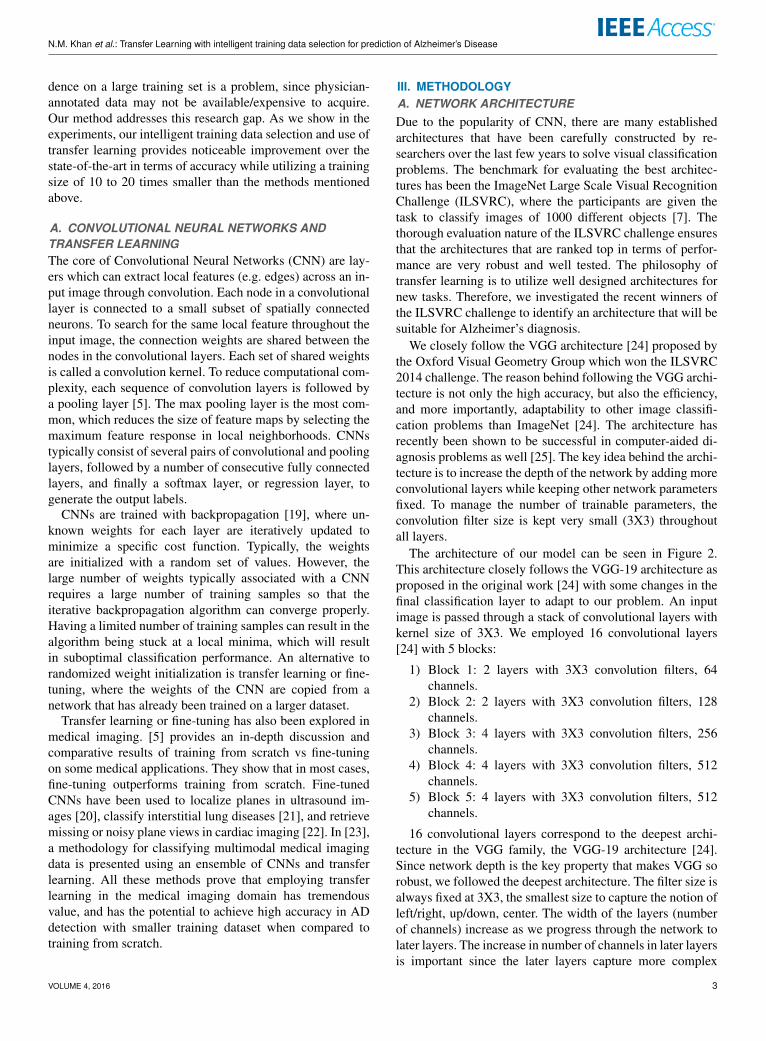
In most applications of transfer learning, the convolutionallayers are used as feature extractors and kept fixed, andonly the fully-connected layer(s) are trained on the trainingdata [5]. However, in our specific application scenario, weare employing an network pre-trained on natural images toclassify medical images. Since the application domains areslightly different, we investigated whether layer-wise transferlearning has an effect on our dataset, and how it relates to thetraining size. To employ layer-wise transfer learning [5], weprogressively “froze” groups of convolutional layers in ourarchitecture. We test four different configurations as seen inFigure 3:

1) Group 1: Convolutional layers 1-4 are frozen.2) Group 2: Convolutional layers 1-8 are frozen.3) Group 3: Convolutional layers 1-12 are frozen.4) Group 4: All convolutional layers (1-16) are frozen.

As we can see, this grouping closely follows the blocksdefined by our architecture. Blocks 1 and 2 are frozen to-gether to form Group 1. We have seen that freezing Block

Conv

(64)

Conv

(64)

po

olin

g

Conv

(128)

Conv

(128)

Conv

(256)

Conv

(256)

Conv

(256)

Conv

(256)

Conv

(512)

Conv

(512)

Conv

(512)

Conv

(512)

Conv

(512)

Conv

(512)

Conv

(512)

Conv

(512)

po

olin

g

po

olin

gp

oo

ling

po

olin

g

FC

(256)

FC

(1)

Frozen

Trainable

Conv

(64)

Conv

(64)

po

olin

g

Conv

(128)

Conv

(128)

Conv

(256)

Conv

(256)

Conv

(256)

Conv

(256)

Conv

(512)

Conv

(512)

Conv

(512)

Conv

(512)

Conv

(512)

Conv

(512)

Conv

(512)

Conv

(512)

po

olin

g

po

olin

gp

oo

ling

po

olin

g

FC

(256)

FC

(1)

Frozen

Trainable

(a) Group 1 (b) Group 2

Conv

(64)

Conv

(64)

po

olin

g

Conv

(128)

Conv

(128)

Conv

(256)

Conv

(256)

Conv

(256)

Conv

(256)

Conv

(512)

Conv

(512)

Conv

(512)

Conv

(512)

Conv

(512)

Conv

(512)

Conv

(512)

Conv

(512)

po

olin

g

po

olin

gp

oo

ling

po

olin

g

FC

(256)

FC

(1)

Frozen

Trainable

(c) Group 3

Conv

(64)

Conv

(64)

po

olin

g

Conv

(128)

Conv

(128)

Conv

(256)

Conv

(256)

Conv

(256)

Conv

(256)

Conv

(512)

Conv

(512)

Conv

(512)

Conv

(512)

Conv

(512)

Conv

(512)

Conv

(512)

Conv

(512)

po

olin

g

po

olin

gp

oo

ling

po

olin

g

FC

(256)

FC

(1)

Frozen

Trainable

(d) Group 4

FIGURE 3: The 4 configurations used for layer-wise transferlearning.

1 and 2 separately does not have any noticeable effect onresults (difference of average accuracy in the range of 0.05-0.45% for our dataset). Since Block 1 consists of the lowestconvolutional layers which serve as low-level feature extrac-tors [6], freezing Block 1 separately from Block 2 does notprovide any noticeable improvement. Hence, to speed up theexperimental process, we opted for the aforementioned fourconfigurations.

B. MOST INFORMATIVE TRAINING DATA SELECTION

While transfer learning provides an opportunity to usesmaller set of training data, choosing the best possible datafor training is still critical to the success of the overallmethod. Typically, from a 3D MRI scan, we have a largenumber of images that we can choose from. In most recentmethods, the images to be used for training are extracted atrandom. Instead, in our proposed method, we extract the mostinformative slices to train the network. For this, we calculatethe image entropy of each slice. In general, for a set of Msymbols with probabilities p1, p2, . . . , pM the entropy can be

4 VOLUME 4, 2016


calculated as follows [28]:

H = −M∑i=1

pi log pi. (1)

For an image (a single slice), the entropy can be similarlycalculated from the histogram [28]. The entropy provides ameasure of variation in a slice. The higher the entropy of animage, the more information it contains. However, entropyis highly susceptible to noise [29], and will not work wellfor a generic image dataset. But in this application scenario,the images have already gone through some preprocessingfor noise removal [18], and all the images are standardized.Hence, if we sort the slices in terms of entropy in descendingorder, the slices with the highest entropy values can beconsidered as the most informative images, and using theseimages for training will provide robustness.

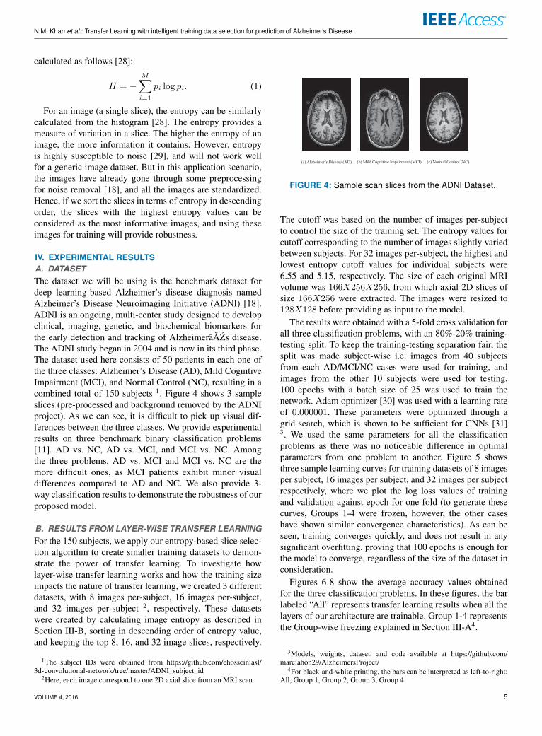
IV. EXPERIMENTAL RESULTSA. DATASETThe dataset we will be using is the benchmark dataset fordeep learning-based Alzheimer’s disease diagnosis namedAlzheimer’s Disease Neuroimaging Initiative (ADNI) [18].ADNI is an ongoing, multi-center study designed to developclinical, imaging, genetic, and biochemical biomarkers forthe early detection and tracking of AlzheimerâAZs disease.The ADNI study began in 2004 and is now in its third phase.The dataset used here consists of 50 patients in each one ofthe three classes: Alzheimer’s Disease (AD), Mild CognitiveImpairment (MCI), and Normal Control (NC), resulting in acombined total of 150 subjects 1. Figure 4 shows 3 sampleslices (pre-processed and background removed by the ADNIproject). As we can see, it is difficult to pick up visual dif-ferences between the three classes. We provide experimentalresults on three benchmark binary classification problems[11]. AD vs. NC, AD vs. MCI, and MCI vs. NC. Amongthe three problems, AD vs. MCI and MCI vs. NC are themore difficult ones, as MCI patients exhibit minor visualdifferences compared to AD and NC. We also provide 3-way classification results to demonstrate the robustness of ourproposed model.

B. RESULTS FROM LAYER-WISE TRANSFER LEARNINGFor the 150 subjects, we apply our entropy-based slice selec-tion algorithm to create smaller training datasets to demon-strate the power of transfer learning. To investigate howlayer-wise transfer learning works and how the training sizeimpacts the nature of transfer learning, we created 3 differentdatasets, with 8 images per-subject, 16 images per-subject,and 32 images per-subject 2, respectively. These datasetswere created by calculating image entropy as described inSection III-B, sorting in descending order of entropy value,and keeping the top 8, 16, and 32 image slices, respectively.

1The subject IDs were obtained from https://github.com/ehosseiniasl/3d-convolutional-network/tree/master/ADNI_subject_id

2Here, each image correspond to one 2D axial slice from an MRI scan

(a) Alzheimer’s Disease (AD) (b) Mild Cognitive Impairment (MCI) (c) Normal Control (NC)

FIGURE 4: Sample scan slices from the ADNI Dataset.

The cutoff was based on the number of images per-subjectto control the size of the training set. The entropy values forcutoff corresponding to the number of images slightly variedbetween subjects. For 32 images per-subject, the highest andlowest entropy cutoff values for individual subjects were6.55 and 5.15, respectively. The size of each original MRIvolume was 166X256X256, from which axial 2D slices ofsize 166X256 were extracted. The images were resized to128X128 before providing as input to the model.

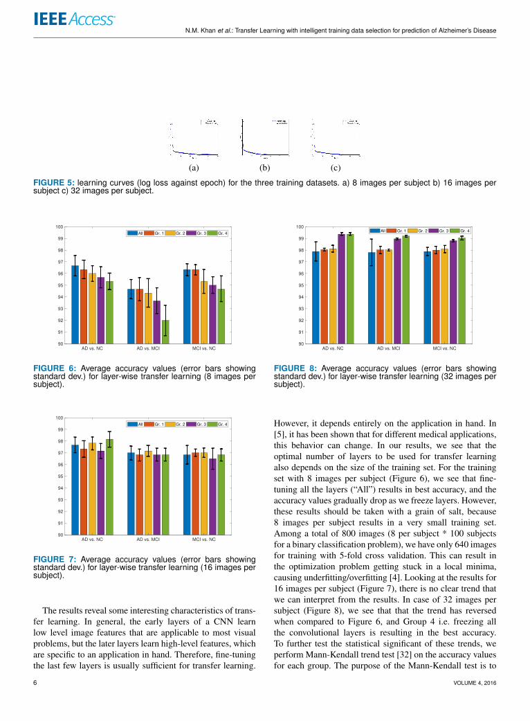
The results were obtained with a 5-fold cross validation forall three classification problems, with an 80%-20% training-testing split. To keep the training-testing separation fair, thesplit was made subject-wise i.e. images from 40 subjectsfrom each AD/MCI/NC cases were used for training, andimages from the other 10 subjects were used for testing.100 epochs with a batch size of 25 was used to train thenetwork. Adam optimizer [30] was used with a learning rateof 0.000001. These parameters were optimized through agrid search, which is shown to be sufficient for CNNs [31]3. We used the same parameters for all the classificationproblems as there was no noticeable difference in optimalparameters from one problem to another. Figure 5 showsthree sample learning curves for training datasets of 8 imagesper subject, 16 images per subject, and 32 images per subjectrespectively, where we plot the log loss values of trainingand validation against epoch for one fold (to generate thesecurves, Groups 1-4 were frozen, however, the other caseshave shown similar convergence characteristics). As can beseen, training converges quickly, and does not result in anysignificant overfitting, proving that 100 epochs is enough forthe model to converge, regardless of the size of the dataset inconsideration.

Figures 6-8 show the average accuracy values obtainedfor the three classification problems. In these figures, the barlabeled “All” represents transfer learning results when all thelayers of our architecture are trainable. Group 1-4 representsthe Group-wise freezing explained in Section III-A4.

3Models, weights, dataset, and code available at https://github.com/marciahon29/AlzheimersProject/

4For black-and-white printing, the bars can be interpreted as left-to-right:All, Group 1, Group 2, Group 3, Group 4

VOLUME 4, 2016 5

https://github.com/ehosseiniasl/3d-convolutional-network/tree/master/ADNI_subject_id

https://github.com/ehosseiniasl/3d-convolutional-network/tree/master/ADNI_subject_id

https://github.com/marciahon29/AlzheimersProject/



(a) (b) (c)

FIGURE 5: learning curves (log loss against epoch) for the three training datasets. a) 8 images per subject b) 16 images persubject c) 32 images per subject.

AD vs. NC AD vs. MCI MCI vs. NC

90

91

92

93

94

95

96

97

98

99

100

All Gr. 1 Gr. 2 Gr. 3 Gr. 4

FIGURE 6: Average accuracy values (error bars showingstandard dev.) for layer-wise transfer learning (8 images persubject).


90

91

92

93

94

95

96

97

98

99

100

All Gr. 1 Gr. 2 Gr. 3 Gr. 4


The results reveal some interesting characteristics of trans-fer learning. In general, the early layers of a CNN learnlow level image features that are applicable to most visualproblems, but the later layers learn high-level features, whichare specific to an application in hand. Therefore, fine-tuningthe last few layers is usually sufficient for transfer learning.


90

91

92

93

94

95

96

97

98

99

100All Gr. 1 Gr. 2 Gr. 3 Gr. 4


However, it depends entirely on the application in hand. In[5], it has been shown that for different medical applications,this behavior can change. In our results, we see that theoptimal number of layers to be used for transfer learningalso depends on the size of the training set. For the trainingset with 8 images per subject (Figure 6), we see that fine-tuning all the layers (“All”) results in best accuracy, and theaccuracy values gradually drop as we freeze layers. However,these results should be taken with a grain of salt, because8 images per subject results in a very small training set.Among a total of 800 images (8 per subject * 100 subjectsfor a binary classification problem), we have only 640 imagesfor training with 5-fold cross validation. This can result inthe optimization problem getting stuck in a local minima,causing underfitting/overfitting [4]. Looking at the results for16 images per subject (Figure 7), there is no clear trend thatwe can interpret from the results. In case of 32 images persubject (Figure 8), we see that that the trend has reversedwhen compared to Figure 6, and Group 4 i.e. freezing allthe convolutional layers is resulting in the best accuracy.To further test the statistical significant of these trends, weperform Mann-Kendall trend test [32] on the accuracy valuesfor each group. The purpose of the Mann-Kendall test is to

6 VOLUME 4, 2016


identify if there are any monotonic trends in a series of data.The hypothesis of the test is that there are no trends in thedata. A low P-value from the test means that we can reject thenull hypothesis and say with confidence that there is indeeda monotonic trend.

Problem P-Value(8 per sub)

P-Value(16 per sub)

P-Value(32 per sub)

AD vs. NC 0.0275 0.8065 0.05AD vs. MCI 0.05 1.0 0.05MCI vs. NC 0.05 0.8065 0.0275

TABLE 1: P-values obtained from Mann-Kendall test on allthe classification problems.

Table 1 reports the results of the Mann-Kendall test oneach individual classification problem for the 3 test sets wehave. The P-values were obtained by running the test onall the 5 group values for each problem (e.g. for 8-imagesper subject and AD vs. NC classification problem, the fivevalues from the left-most five bars of Figure 6 were fedto the Mann-Kendall algorithm to see whether there is atrend). As we can see, for 8-images per subject and 32-images per subject, the low P values indicate that there isindeed decreasing/increasing trend present, while for the 16-images per subject case, the high P-values indicate that notrend was observed. The conclusion we draw from this isthat the application in hand for us has visual similarity tonatural images, on which the network is pre-trained. As aresult, with sufficient training data of 32 images per subject,only fine-tuning the fully-connected layers is enough. This isalso encouraging from a practical perspective, since trainingfewer layers means fewer parameters to optimize, which, inturns, will result in a faster training process.

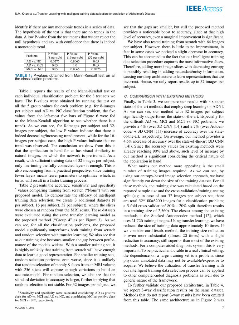
Table 2 presents the accuracy, sensitivity, and specificity5 values comparing training from scratch (“None”) with ourproposed model. To demonstrate the efficacy of intelligenttraining data selection, we create 3 additional datasets (8per subject, 16 per subject, 32 per subject), where the sliceswere chosen at random from the MRI scans. These datasetswere evaluated using the same transfer learning model asthe proposed method (“Group 4” as per Figure 3). As wecan see, for all the classification problems, the proposedmodel significantly outperforms both training from scratchand random selection with transfer learning. We also see thatas our training size becomes smaller, the gap between perfor-mance of the models widens. With a smaller training set, itis highly unlikely that training from scratch will have enoughdata to learn a good representation. For smaller training sets,random selection performs even worse, since it is unlikelythat random selection of merely 8 slices from an MRI volumewith 256 slices will capture enough variations to build anaccurate model. For random selection, we also see that thestandard deviation in accuracy is larger, further implying thatrandom selection is not stable. For 32 images per subject, we

5Sensitivity and specificity were calculated cosnidering AD as positiveclass for AD vs. MCI and AD vs. NC, and considering MCI as positive classfor MCI vs. NC, respectively.

see that the gaps are smaller, but still the proposed methodprovides a noticeable boost to accuracy, since at that highlevel of accuracy, even a marginal improvement is significant.

We have also tested training from scratch with 64 imagesper subject. However, there is little to no improvement, infact in some cases we noticed a slight decrease in accuracy.This can be accounted to the fact that our intelligent trainingdata selection procedure captures the most informative slices.Therefore, adding more image slices with decreasing entropyis possibly resulting in adding redundant/noisy information,causing our deep architecture to learn representations that areincorrect. Hence, we only report results up to 32 images persubject.

C. COMPARISON WITH EXISTING METHODSFinally, in Table 3, we compare our results with six otherstate-of-the-art methods that employ deep learning on ADNI.As we can see, our method with 32 images per subjectsignificantly outperforms the state-of-the-art. Especially forthe difficult AD vs. MCI and MCI vs. NC problems, weprovide a 4% (over 3D CNN [14]) and a 7% (over Autoen-coder + 3D CNN [11]) increase of accuracy over the state-of-the-art, respectively. On average, our method provides a4.5% increase of accuracy over the state-of-the-art (3D CNN[14]). Since the accuracy values for existing methods werealready reaching 90% and above, such level of increase byour method is significant considering the critical nature ofthe application in hand.

What makes our method more appealing is the smallnumber of training images required. As we can see, byusing our entropy-based image selection approach, we havesignificantly cut down the size of the training dataset. For allthese methods, the training size was calculated based on thereported sample size and the cross-validation/training-testingsplit (e.g. in case of our 32 images per subject set, thereare total 32*100=3200 images for a classification problem;a 5-fold cross-validation/ 80% - 20% split therefore resultsin a training size of 2,560). The closest among the existingmethods is the Stacked Autoencoder method [12], whichuses 21,726 training images. Using transfer learning, we havereduced the size of training data approximately 10 times. Ifwe consider our 16/sub. method, the training size reductionis even more substantial (almost 20 times) with a slightreduction in accuracy; still superior than most of the existingmethods. For a computer-aided diagnosis system this is veryimportant. To be practical and usable in a real clinical setting,the dependence on a large training set is a problem, sincephysician annotated data may not be available/expensive toacquire. We believe the utilization of transfer learning withour intelligent training data selection process can be appliedto other computer-aided diagnosis problems as well due togeneric nature of the framework.

To further validate our proposed architecture, in Table 4,we report 3-way classification results on the same dataset.Methods that do not report 3-way results have been omittedfrom this table. The same architecture as in Figure 2 was

VOLUME 4, 2016 7


AD vs. NC AD vs. MCI MCI vs. NC# Images (Model) Acc. Sens. Spec. Acc. Sens. Spec. Acc. Sens. Spec.8 per sub (None) 79.67 (3.71) 83.2 76.1 65.67 (2.37) 63.2 68.1 75 (2.19) 73.2 76.88 per sub (TL+Random) 67.69 (7.71) 63.2 72.2 59.21 (5.47) 63.4 55 69.2 (2.19) 73.2 65.28 per sub (Proposed) 95.34 (0.7) 96.1 94.6 92 (1.3) 93.1 90.9 94.67 (1.1) 95.2 94.116 per sub (None) 90.5 (2.24) 90.8 90.2 81.17 (3.14) 83.6 78.7 87.335 (2.43) 88.2 86.516 per sub (TL+Random) 84.7 (4.21) 86.4 83 74.21 (4.17) 73.1 75.3 81.7 (1.7) 83.1 80.316 per sub (Proposed) 98.17 (0.65) 97.1 99.2 96.84 (0.55) 95.7 98 96.83 (0.53) 97.1 96.632 per sub (None) 96.4(2.02) 95.6 97.2 97.14 (1.29) 95.9 98.4 97.12 (1.3) 96.1 98.132 per sub (TL+Random) 91.1(2.9) 92.2 90 92.33 (2.21) 93.5 91.2 93.22 (2.1) 92.1 94.332 per sub (Proposed) 99.36 (0.1) 98.7 100 99.2 (0.8) 98.9 99.5 99.04 (0.15) 99.5 98.6

TABLE 2: Comparison of accuracy, sensitivity and specificity values (in %) without transfer learning (“None”), transfer learning+ random selection (“TL+Random”), and proposed transfer learning + intelligent selection (“Proposed”). Best accuracy for eachset of training dataset in bold. Standard deviation of accuracy in brackets.

Method Training Size(# images) AD vs. NC AD vs. MCI MCI vs. NC Average

StackedAutoencoder [12] 21,726 87.76 - 76.92 -

Patch-basedAutoencoder [10] 103,683 94.74 88.1 86.35 89.73

MultitaskLearning [15] 29,880 91.4 70.1 77.4 79.63

Autoencoder+ 3D CNN [11] 117,708 95.39 86.84 92.11 91.45

3D CNN [14] 39,942 97.6 95 90.8 94.47Inception [13] 46,751 98.84 - - -Our Method(16/sub.) 1,280 98.17 96.84 96.83 97.28

Our Method(32/sub.) 2,560 99.36 99.2 99.04 99.2

TABLE 3: Comparison of accuracy values (in %). Best method in bold, second best in italic.

Method AD vs. MCI vs. NCPatch-basedAutoencoder [10] 85

Autoencoder+ 3D CNN [11] 89.47

3D CNN [14] 89.1Our Method(32/sub.) 95.19

TABLE 4: Comparison of accuracy values for 3-way classifi-cation (in %). Best method in bold, second best in italic.

used, the only change was the final classification layer, whichwas modified to be able to perform 3-way classification.The same 5-fold cross validation with an 80%-20% training-testing split was utilized for 3-way classification. As can beseen, even for 3-way classification, we achieve state-of-the-art results when compared to existing approaches, provingthe effectiveness of our method.

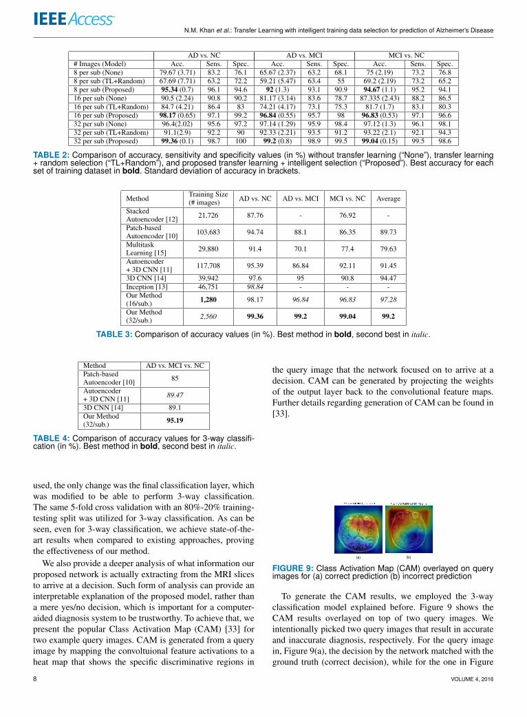
We also provide a deeper analysis of what information ourproposed network is actually extracting from the MRI slicesto arrive at a decision. Such form of analysis can provide aninterpretable explanation of the proposed model, rather thana mere yes/no decision, which is important for a computer-aided diagnosis system to be trustworthy. To achieve that, wepresent the popular Class Activation Map (CAM) [33] fortwo example query images. CAM is generated from a queryimage by mapping the convoltuional feature activations to aheat map that shows the specific discriminative regions in

the query image that the network focused on to arrive at adecision. CAM can be generated by projecting the weightsof the output layer back to the convolutional feature maps.Further details regarding generation of CAM can be found in[33].

(a) (b)

FIGURE 9: Class Activation Map (CAM) overlayed on queryimages for (a) correct prediction (b) incorrect prediction

To generate the CAM results, we employed the 3-wayclassification model explained before. Figure 9 shows theCAM results overlayed on top of two query images. Weintentionally picked two query images that result in accurateand inaccurate diagnosis, respectively. For the query imagein, Figure 9(a), the decision by the network matched with theground truth (correct decision), while for the one in Figure

8 VOLUME 4, 2016


9(b), the network’s prediction was incorrect. In the CAMheatmap, the more red a region is, the higher attention itreceived from the model.

These results reveal some interesting aspects of the pro-posed model. For the correct prediction (Figure 9(a)), we seethat the regions containing Gray Matter (GM) and CerebralSpinal Fluid (CSF) received more attention from the net-work. This aligns with the neuropathology of Alzheimer’sdiagnosis. It is known that Alzheimer’s results in significantatrophy in the GM regions, with an increased amount of CSF[10], [34]. Indeed, our network is focusing on those regionsto arrive at the correct decision. However, for the incorrectprediction (Figure 9(b)), we see that the background to scantransition regions received more attention, likely due to thepoor contrast in the MRI itself in this particular slice. Thistells us that the network failed to provide a correct diagnosisdue to its inability to extract accurate features. If a doctorwas presented with an interpretable output like this, theywill instantly be able to tell why exactly the proposed modelfailed, making the overall framework more trustworthy.

V. CONCLUSIONIn this paper, we propose a transfer learning-based methodfor Alzheimer’s diagnosis from MRI images. We hypothesizethat adopting a robust and proven architecture for natu-ral images and employing transfer learning with intelligenttraining data selection can not only improve the accuracyof a model, but also reduce reliance on a large trainingset. We validate our hypothesis with detailed experimentson the benchmark ADNI dataset, where MRI scans of 50subjects from each category of AD, MCI, and NC (total 150subjects) were used to obtain accuracy results. We investigatewhether layer-wise transfer learning has an effect on ourapplication by progressively freezing groups of layers in ourarchitecture, and we present in-depth results of layer-wisetransfer learning and its relation to the training data size.Finally, we present comparative results with six other state-of-the-art methods, where our proposed method significantlyoutperforms the others, providing a 4% and a 7% increasein accuracy over the state-of-the-art for AD vs. MCI andMCI vs. NC classification problems, respectively. We alsoreport 3-way classification results, achieving state-of-the-art,proving the robustness of the proposed method.

In future, we will investigate whether the same archi-tecture can be employed to other computer-aided diagnosisproblems. We will also investigate whether our entropy-based image selection method can be improved further byincorporating further probabilistic measures on the images.

Keeping up with the spirit of reproducible research, all ourmodels, dataset, and code can be accessed through the repos-itory at: https://github.com/marciahon29/AlzheimersProject/.

REFERENCES[1] R. Brookmeyer, E. Johnson, K. Ziegler-Graham, and H. M. Arrighi,

“Forecasting the global burden of alzheimer’s disease,” Alzheimer’s &

dementia, vol. 3, no. 3, pp. 186–191, 2007.[2] S. Klöppel, C. M. Stonnington, J. Barnes, F. Chen, C. Chu, C. D. Good,

I. Mader, L. A. Mitchell, A. C. Patel, C. C. Roberts et al., “Accuracyof dementia diagnosis - a direct comparison between radiologists and acomputerized method,” Brain, vol. 131, no. 11, pp. 2969–2974, 2008.

[3] C. Plant, S. J. Teipel, A. Oswald, C. Böhm, T. Meindl, J. Mourao-Miranda,A. W. Bokde, H. Hampel, and M. Ewers, “Automated detection of brainatrophy patterns based on mri for the prediction of alzheimer’s disease,”Neuroimage, vol. 50, no. 1, pp. 162–174, 2010.

[4] D. Erhan, P.-A. Manzagol, Y. Bengio, S. Bengio, and P. Vincent, “Thedifficulty of training deep architectures and the effect of unsupervised pre-training,” in Artificial Intelligence and Statistics, 2009, pp. 153–160.

[5] N. Tajbakhsh, J. Y. Shin, S. R. Gurudu, R. T. Hurst, C. B. Kendall,M. B. Gotway, and J. Liang, “Convolutional neural networks for medicalimage analysis: Full training or fine tuning?” IEEE transactions on medicalimaging, vol. 35, no. 5, pp. 1299–1312, 2016.

[6] J. Yosinski, J. Clune, Y. Bengio, and H. Lipson, “How transferable arefeatures in deep neural networks?” in Advances in neural informationprocessing systems, 2014, pp. 3320–3328.

[7] O. Russakovsky, J. Deng, H. Su, J. Krause, S. Satheesh, S. Ma, Z. Huang,A. Karpathy, A. Khosla, M. Bernstein et al., “Imagenet large scale visualrecognition challenge,” International Journal of Computer Vision, vol. 115,no. 3, pp. 211–252, 2015.

[8] M. Long, Y. Cao, J. Wang, and M. I. Jordan, “Learning transferablefeatures with deep adaptation networks,” arXiv preprint arXiv:1502.02791,2015.

[9] D. Jha, J.-I. Kim, and G.-R. Kwon, “Diagnosis of alzheimer’s diseaseusing dual-tree complex wavelet transform, pca, and feed-forward neuralnetwork,” Journal of Healthcare Engineering, vol. 2017, 2017.

[10] A. Gupta, M. Ayhan, and A. Maida, “Natural image bases to representneuroimaging data,” in International Conference on Machine Learning,2013, pp. 987–994.

[11] A. Payan and G. Montana, “Predicting alzheimer’s disease: a neu-roimaging study with 3d convolutional neural networks,” arXiv preprintarXiv:1502.02506, 2015.

[12] S. Liu, S. Liu, W. Cai, S. Pujol, R. Kikinis, and D. Feng, “Early diagnosisof alzheimer’s disease with deep learning,” in Biomedical Imaging (ISBI),2014 IEEE 11th International Symposium on. IEEE, 2014, pp. 1015–1018.

[13] S. Sarraf, G. Tofighi et al., “Deepad: Alzheimer’s disease classificationvia deep convolutional neural networks using mri and fmri,” bioRxiv, p.070441, 2016.

[14] E. Hosseini-Asl, R. Keynton, and A. El-Baz, “Alzheimer’s disease diag-nostics by adaptation of 3d convolutional network,” in Image Processing(ICIP), 2016 IEEE International Conference on. IEEE, 2016, pp. 126–130.

[15] F. Li, L. Tran, K.-H. Thung, S. Ji, D. Shen, and J. Li, “A robust deep modelfor improved classification of ad/mci patients,” IEEE journal of biomedicaland health informatics, vol. 19, no. 5, pp. 1610–1616, 2015.

[16] Y. Zhang, H. Zhang, X. Chen, M. Liu, X. Zhu, S.-W. Lee, and D. Shen,“Strength and similarity guided group-level brain functional networkconstruction for mci diagnosis,” Pattern Recognition, vol. 88, pp. 421–430,2019.

[17] Y. Zhang, H. Zhang, X. Chen, S.-W. Lee, and D. Shen, “Hybrid high-order functional connectivity networks using resting-state functional mrifor mild cognitive impairment diagnosis,” Scientific reports, vol. 7, no. 1,p. 6530, 2017.

[18] C. R. Jack, M. A. Bernstein, N. C. Fox, P. Thompson, G. Alexander,D. Harvey, B. Borowski, P. J. Britson, J. L Whitwell, C. Ward et al., “Thealzheimer’s disease neuroimaging initiative (adni): Mri methods,” Journalof magnetic resonance imaging, vol. 27, no. 4, pp. 685–691, 2008.

[19] J. Schmidhuber, “Deep learning in neural networks: An overview,” Neuralnetworks, vol. 61, pp. 85–117, 2015.

[20] H. Chen, D. Ni, J. Qin, S. Li, X. Yang, T. Wang, and P. A. Heng, “Standardplane localization in fetal ultrasound via domain transferred deep neuralnetworks,” IEEE journal of biomedical and health informatics, vol. 19,no. 5, pp. 1627–1636, 2015.

[21] M. Gao, U. Bagci, L. Lu, A. Wu, M. Buty, H.-C. Shin, H. Roth, G. Z. Pa-padakis, A. Depeursinge, R. M. Summers et al., “Holistic classification ofct attenuation patterns for interstitial lung diseases via deep convolutionalneural networks,” Computer Methods in Biomechanics and BiomedicalEngineering: Imaging & Visualization, pp. 1–6, 2016.

[22] J. Margeta, A. Criminisi, R. Cabrera Lozoya, D. C. Lee, and N. Ayache,“Fine-tuned convolutional neural nets for cardiac mri acquisition plane

VOLUME 4, 2016 9



recognition,” Computer Methods in Biomechanics and Biomedical Engi-neering: Imaging & Visualization, vol. 5, no. 5, pp. 339–349, 2017.

[23] A. Kumar, J. Kim, D. Lyndon, M. Fulham, and D. Feng, “An ensembleof fine-tuned convolutional neural networks for medical image classifica-tion,” IEEE journal of biomedical and health informatics, vol. 21, no. 1,pp. 31–40, 2017.

[24] K. Simonyan and A. Zisserman, “Very deep convolutional networks forlarge-scale image recognition,” arXiv preprint arXiv:1409.1556, 2014.

[25] J.-H. Lee, D.-h. Kim, S.-N. Jeong, and S.-H. Choi, “Diagnosis and pre-diction of periodontally compromised teeth using a deep learning-basedconvolutional neural network algorithm,” Journal of periodontal & implantscience, vol. 48, no. 2, pp. 114–123, 2018.

[26] A. Krizhevsky, I. Sutskever, and G. E. Hinton, “Imagenet classificationwith deep convolutional neural networks,” in Advances in neural informa-tion processing systems, 2012, pp. 1097–1105.

[27] F. Chollet, Deep learning with python. Manning Publications Co., 2017.[28] C. Studholme, D. L. Hill, and D. J. Hawkes, “An overlap invariant entropy

measure of 3d medical image alignment,” Pattern recognition, vol. 32,no. 1, pp. 71–86, 1999.

[29] D.-Y. Tsai, Y. Lee, and E. Matsuyama, “Information entropy measure forevaluation of image quality,” Journal of digital imaging, vol. 21, no. 3, pp.338–347, 2008.

[30] D. P. Kingma and J. Ba, “Adam: A method for stochastic optimization,”arXiv preprint arXiv:1412.6980, 2014.

[31] J. S. Bergstra, R. Bardenet, Y. Bengio, and B. Kégl, “Algorithms for hyper-parameter optimization,” in Advances in neural information processingsystems, 2011, pp. 2546–2554.

[32] D. Helsel and R. Hirsch, “Statistical methods in water resources techniquesof water resources investigations, book 4, chapter a3,” US geologicalsurvey. Retrieved from http://pubs. usgs. gov/twri/twri4a3, 2002.

[33] B. Zhou, A. Khosla, A. Lapedriza, A. Oliva, and A. Torralba, “Learningdeep features for discriminative localization,” in Proceedings of the IEEEconference on computer vision and pattern recognition, 2016, pp. 2921–2929.

[34] S. L. Risacher and A. J. Saykin, “Neuroimaging and other biomarkers foralzheimer’s disease: the changing landscape of early detection,” Annualreview of clinical psychology, vol. 9, pp. 621–648, 2013.

DR. NAIMUL MEFRAZ KHAN (M’11) is anassistant professor in the Department of Elec-trical, Computer & Biomedical Engineering andthe Master of Digital Media program at Ryer-son University. He obtained his PhD in Electricaland Computer Engineering, M.Sc., and B.Sc. inComputer Science from Ryerson University, theUniversity of Windsor, and Bangladesh Universityof Engineering & Technology, respectively. Hisresearch focuses on creating user-centric intelli-

gent systems through the combination of novel machine learning, computervision algorithms and human-computer interaction mechanisms. He is arecipient of the best paper award at the IEEE International Symposiumon Multimedia, the OCE TalentEdge Postdoctoral Fellowship, the OntarioGraduate Scholarship, and several other awards. He is a member of the IEEESignal Processing Society and the ACM SIGGRAPH Toronto chapter.

NABILA ABRAHAM (M’16) is an MASc studentat the Ryerson Multimedia Laboratory at RyersonUniversity. She completed her BEng. in Biomed-ical Engineering from Ryerson University. Herresearch focuses on using deep learning to creategeneralizable models for medical image analysis.

MARCIA HON is a recent Master’s graduate ofData Science and Analytics from Ryerson Univer-sity. She presented her MasterâAZs work at theIEEE BIBM Conference in 2017. Her interestsare in Data Science and Analytics as applied tothe Medical Sciences. Currently, she works in theKrembil Centre for Neuroinformatics at the Centrefor Addiction and Mental Health (CAMH).

10 VOLUME 4, 2016

Documents

Transfer Learning with intelligent training data selection ... · we pick the training data that would provide the most amount of information through image entropy. We show that through