Embed Size (px)
Citation preview
DEPARTMENT OF ECONOMICS
REVISITING MONEY-OUTPUT CAUSALITY
FROM A BAYESIAN LOGISTIC SMOOTH
TRANSITION VECM PERSPECTIVE
Deborah Gefang, University of Leicester, UK
Working Paper No. 08/5 January 2008
Revisiting money-output causality from a Bayesian
logistic smooth transition VECM perspective
Deborah Gefang ∗
Department of EconomicsUniversity of Leicester
UK
January 29, 2008
Abstract
This paper proposes a Bayesian approach to explore money-outputcausality within a logistic smooth transition VECM framework. Ourempirical results provide substantial evidence that the postwar USmoney-output relationship is nonlinear, with regime changes mainlygoverned by the lagged inflation rates. More importantly, we ob-tain strong support for long-run non-causality and nonlinear Granger-causality from money to output. Furthermore, our impulse responseanalysis reveals that a shock to money appears to have negative accu-mulative impact on real output over the next fifty years, which callsfor more caution when using money as a policy instrument.
∗This paper has benefited from the helpful discussions with Stephen Hall, Gary Koop,Roberto Leon-Gonzalez, Roderick McCrorie, Emi Mise and Rodney Strachan. Any re-maining errors are the author’s responsibility. Financial support from the Department ofEconomics, University of Leicester is gratefully acknowledged.
1
1 Introduction
From the late 1980s through the early 2000s, with the prevalence of interest
rate based Taylor rule (Taylor, 1993), the role of money (monetary base or
monetary aggregates) had been deemphasized in much research on monetary
policy and macroeconomic modeling (see, e.g., Barro (1989), Taylor (1999),
Clarida, Galı and Gertler (2000)). However, there has been a renewed in-
terest in the effect of money in recent years. Meltzer (2001), Nelson (2002,
2003), Duca and VanHoose (2004), among others, raise the issue that money
constitutes a crucial channel for the transmission mechanism of monetary
policy, and the role of money cannot be simply replaced by any other policy
instruments. Moreover, we find money reemerges as an important variable
of concern in a number of most recent empirical monetary analysis (for in-
stance, Wang and Wen (2005), Sims and Zha (2006), Hill (2007), to mention
a few).1
This paper contributes to the discussion on whether money matters by
revisiting an old topic: examining the causal effects from money to output
in the postwar US data.2 However, the current research departs from the
literature in two main aspects. First, to capture the possible regime changes
in US monetary policy, we adopt a smooth transition vector error correction1As of the time of writing, Federal Reserve, the European Central Bank, Bank of
England and central banks from Canada and Switzerland jointly announced cash injectionplans to lessen the credit squeeze triggered by the sub-prime mortgages losses. Althoughthe consequence of the intervention is yet to know, this unprecedent operation clearlyimplies that money remains a vital instrument for monetary policy.
2The money-output relationship has been intensively investigated in the literature.However, there is much less consensus about how money affects output (see, e.g. Sims(1972, 1980), Stock and Watson (1989), King and Watson (1997), Coe and Nason (2004)).
2
model (STVECM) incorporating cointegration of an unknown form. Second,
we develop a simple Bayesian approach to investigating the causal effects
from money to output.
Single-equation smooth transition error correction models have been
widely used in the literature to capture the possible nonlinear money-output
relationship (Lutekepohl, Terasvirta and Wolters (1999), Terasvirta and
Eliasson (2001), Escribano (2004), Haug and Tam (2007), to mention a
few). However, considering the interplay between endogenously determined
money, interest rates and the ultimate policy targets output and inflation,
we believe STVECM can be more effective in capturing both the long run
and short run dynamics in the linkages among all the variables. Perhaps
the reason why researchers have not followed this route is due to the lack of
a fully developed statistics tool that can directly test the cointegration (or
no cointegration) null in a nonlinear VECM against its both linear and non-
linear alternatives (see Seo (2004), Seo (2006), Kapetanios, Shin and Snell
(2006) for details). In the literature, only Rothman, van Dijk and Frances
(2001) apply a multivariate STVECM framework which is closest to us to
study the money-output relationship.3 Yet, Rothman, van Dijk and Frances
(2001) pre-impose a theory based long-run cointegrating relationship in their
estimation. While recognizing that the actual money-output interrelation is
rather complex, unlike Rothman, van Dijk and Frances (2001), we let both
the cointegration rank and cointegrating vectors to be determined by the
data.3Rothman, van Dijk and Frances (2001) test Granger causality from money to output
in a classical context involving rolling window forecasting.
3
Our estimation technique is Bayesian. Specifically, we extend the Bayesian
cointegration space approach introduced in Strachan and Inder (2004) and
collapsed Gibbs sampler developed in Koop, Leon-Gonzalez and Strachan
(2005) into the nonlinear framework. Our method jointly captures the equi-
librium and presence of nonlinearity in the STVECM in a single step. Com-
pared with the available classical estimation techniques which often require
multiple steps and Taylor expansions, our approach is less susceptible to the
sequential testing and inaccurate approximation problems. Furthermore,
the commonly used maximum likelihood estimation in classical works is
subject to the multi-mode problem caused by the nuisance parameters in
the transition function of the STVECM. Yet, jagged likelihood functions do
not create any particular problems in our Gibbs sampling scheme.
Considering the large model we employed is subject to the criticism of
being too parameter rich, we use Bayes Factors for model comparison in
order to reward more parsimonious models.4 Alternative models are spec-
ified by placing zero restrictions on certain parameters of the unrestricted
STVECM. Our approach to examining whether money long-run causes out-
put is in spirit to that in Hall and Wickens (1993), Hall and Milne (1994)
and Granger and Lin (1995). With respects to the Granger causality test
from money to output, aside from considering if money directly enters the
output equation as described in Rothman, van Dijk and Frances (2001), we
look into whether money indirectly affects output through the channels of
price and interest rate.4Bayes Factors include an automatic penalty for more complex models (see Koop and
Potter, (1999a, 1999b) for details).
4
An important finding of our study is that the postwar US money-output
relationship is nonlinear, with the regime shifting mainly driven by the
lagged inflation rates. In terms of triggering regime changes, compared
with the key role played by inflation rates, the role of lagged annual growth
rates of output is less important, while the roles played by changes in oil
prices, money and interest rates are nearly negligible. However, it is worth
stressing that, in our study, nonlinear models consistently outperform linear
models.
We find substantial evidence that money does not long-run cause out-
put in the postwar US data. Additionally, consistent with the in-sample
testing results in Rothman, van Dijk and Frances (2001), our studies show
that money is nonlinearly Granger-causal for output. The impulse response
analysis shows that the dynamic paths of output given a shock to money is
rather complex. Most strikingly, we find that the accumulated effect of a
shock to money is negative on real output in the next 50 years, regardless of
the size and sign of the initial shock. This result calls for a word of caution
when using money as a policy instrument.
The outline of this paper is as follows. Section 2 describes the model and
the Bayesian estimation technique. Section 3 reports the empirical results.
Section 4 concludes.
2 STVECM Model and Bayesian Inference
Following a majority of empirical work (for example, Lutekepohl, Terasvirta
and Wolters (1999), Rothman, van Dijk and Frances (2001)), we investigate
5
the money-output relationship in a system of output, money, prices and
interest rates.
We use the monthly US data spanning from 1959:1 to 2006:12. The
data are obtained from the database of Federal Reserve Bank of St. Louis.
Various measures of output, money, prices and interest rates are used in
the literature. In this paper, we adopt the seasonally adjusted industrial
production index (it), the seasonally adjusted M2 money stock (mt), the
producer price index for all commodities (pt), and the secondary market
rate on 3-month Treasury bills (rt) for the measures of output, money, prices
and interest rates, respectively. All variables are in logarithms except for
interest rates which are in percent.
To catch the possible regime changes in US monetary policy, we model
the interrelationship among output, money, prices and interest rates in a
STVECM.5 Let yt = [it mt pt rt], the STVECM of the 1×4 vector time
series process yt, t=1,...,T, conditioning on the p observations t= -p+1,...,0,
can be specified as
4yt =yt−1βα+ ξ + Σph=14yt−hΓh
+ F (zt)(yt−1βzαz + ξz + Σp
h=14yt−hΓzh) + εt
(1)
εt is a Gaussian white noise process where E(εt) = 0, E(ε′sεt) = Σ for s = t,
and E(ε′sεt) = 0 for s 6= t. Note that 4yt = yt−yt−1. The dimensions of Γh
and Γzh are n× n, and the dimensions of β, α′, βz, and αz′ are n× r. Since
5The possible regime changes in US monetary policy have been well documented inthe literature (see, e.g., Weise (1999), Clarida, Galı and Gertler (2000), Leeper and Zha(2003)).
6
we are using monthly data, without loss of generality, we set p = 6.
In model (1), the dynamics of the regime changes are assumed to be
captured by the first order logistic smooth transition function introduced in
Granger and Terasvirta (1993) and Terasvirta (1994):
F (zt) = {1 + exp[−γ(zt − c)/σ]}−1 (2)
where zt is the transition variable determining the regimes. Note that zt
can be any exogenous or endogenous variables of interest. In this paper,
following Rothman, van Dijk and Frances (2001), we set zt to be the lagged
annual growth rates of output, the lagged annual growth rates of money,
the lagged annual inflation rates, the lagged annual changes in interest rates
and the lagged annual growth rates in oil prices, respectively.6 In particular,
we allow the lag length of the transition variables to vary from 1 to 6.
The transition function F (zt) is bounded by 0 and 1. As convention,
we define F (zt) = 0 and F (zt) = 1 corresponding to the lower and upper
regimes, respectively. In function (2), the smoothing parameter γ (which
is non-negative) determines the speed of the smooth transition. Observe
that when γ → ∞, the transition function becomes a Dirac function, then
model (1) becomes a two-regime threshold VECM model along the lines of
Tong (1983). When γ = 0, the logistic function becomes a constant (equal
to 0.5), and the nonlinear model (1) collapses into a linear VECM. The
transition parameter c is the threshold around which the dynamics of the6Rothman, van Dijk and Frances (2001) point out that using annual growth rates
instead of monthly changes as plausible transition variables is in accord with the commonlyaccepted perception that the regimes in the money-output relationship are quite persistent.
7
model change. The value for the parameter σ is chosen by the researcher
and could reasonably be set to one. In this study, we set σ equal to the
standard deviation of the process zt. This effectively normalizes γ such that
we can give γ an interpretation in terms of the inverse of the number of
standard deviations of zt. The transition from one extreme regime to the
other is smooth for reasonable values of γ.
Observe that model (1) encompasses a set of models distinguished by the
number of the long-run equilibrium relationships, the cointegrating vectors,
the order of the autoregressive process, the existence of the nonlinear effects,
the choice of the transition variable, and whether Granger non-causality or
long-run non-causality from money to output is imposed.
2.1 Likelihood Function
Koop, Leon-Gonzalez and Strachan (2005) develop an efficient collapsed
Gibbs sampler for the VECM estimation in linear contexts, which provides
great computation advantages over conventional methods. To incorporate
the collapsed Gibbs sampler into our posterior simulation algorithm, follow-
ing Koop, Leon-Gonzalez and Strachan (2005), we obtain two representa-
tions of the likelihood .
To start with, restricting β and βz to be semi-orthogonal, we write (1)
as
4yt = x1,t−1βα+ x2,tΦ + F (zt)(x1,t−1βzαz + x2,tΦz) + εt (3)
where x1,t−1 = yt−1, x2,t = (1,4yt−1, ...,4yt−p), Φ = (ξ′,Γ′1, ...,Γ
′p)
′, Φz =
(ξz′ ,Γz′1 , ...,Γ
z′p )′. To simplify the notation, we then define the T × n ma-
8
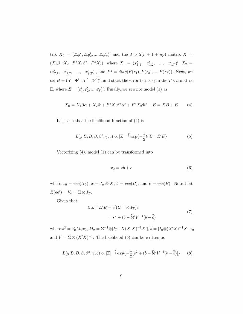
trix X0 = (4y′1,4y′2, ...,4y′T )′ and the T × 2(r + 1 + np) matrix X =
(X1β X2 F zX1βz F zX2), where X1 = (x′1,1, x′1,2, ..., x′1,T )′, X2 =
(x′2,1, x′2,2, ..., x′2,T )′, and F z = diag(F (z1), F (z2), ..., F (zT )). Next, we
set B = (α′ Φ′ αz′ Φz′)′, and stack the error terms εt in the T ×n matrix
E, where E = (ε′1, ε′2, ..., ε
′T )′. Finally, we rewrite model (1) as
X0 = X1βα+X2Φ + F zX1βzαz + F zX2Φz + E = XB + E (4)
It is seen that the likelihood function of (4) is
L(y|Σ, B, β, βz, γ, c) ∝ |Σ|−T2 exp{−1
2trΣ−1E′E} (5)
Vectorizing (4), model (1) can be transformed into
x0 = xb+ e (6)
where x0 = vec(X0), x = In ⊗X, b = vec(B), and e = vec(E). Note that
E(ee′) = Ve = Σ⊗ IT .
Given thattrΣ−1E′E = e′(Σ−1 ⊗ IT )e
= s2 + (b− b)′V −1(b− b)(7)
where s2 = x′0Mvx0,Mv = Σ−1⊗[IT−X(X ′X)−1X ′], b = [In⊗(X ′X)−1X ′]x0
and V = Σ⊗ (X ′X)−1. The likelihood (5) can be written as
L(y|Σ, B, β, βz, γ, c) ∝ |Σ|−T2 exp{−1
2[s2 + (b− b)′V −1(b− b)]} (8)
9
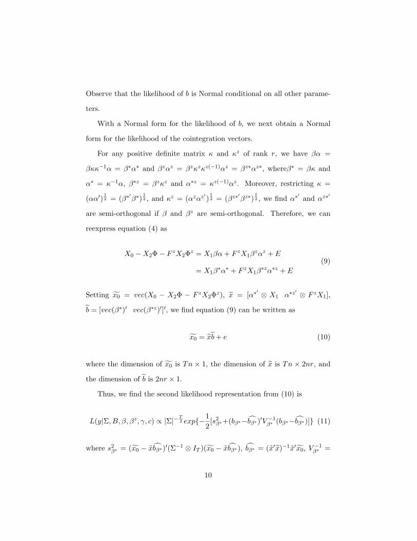
Observe that the likelihood of b is Normal conditional on all other parame-
ters.
With a Normal form for the likelihood of b, we next obtain a Normal
form for the likelihood of the cointegration vectors.
For any positive definite matrix κ and κz of rank r, we have βα =
βκκ−1α = β∗α∗ and βzαz = βzκzκz(−1)αz = βz∗αz∗, whereβ∗ = βκ and
α∗ = κ−1α, β∗z = βzκz and α∗z = κz(−1)αz. Moreover, restricting κ =
(αα′)12 = (β∗′β∗)
12 , and κz = (αzαz′)
12 = (βz∗′βz∗)
12 , we find α∗′ and αz∗′
are semi-orthogonal if β and βz are semi-orthogonal. Therefore, we can
reexpress equation (4) as
X0 −X2Φ− F zX2Φz = X1βα+ F zX1βzαz + E
= X1β∗α∗ + F zX1β
∗zα∗z + E
(9)
Setting x0 = vec(X0 − X2Φ − F zX2Φz), x = [α∗′ ⊗ X1 α∗z′ ⊗ F zX1],
b = [vec(β∗)′ vec(β∗z)′]′, we find equation (9) can be written as
x0 = xb+ e (10)
where the dimension of x0 is Tn × 1, the dimension of x is Tn × 2nr, and
the dimension of b is 2nr × 1.
Thus, we find the second likelihood representation from (10) is
L(y|Σ, B, β, βz, γ, c) ∝ |Σ|−T2 exp{−1
2[s2β∗+(bβ∗−bβ∗)′V −1
β∗ (bβ∗−bβ∗)]} (11)
where s2β∗ = (x0 − xbβ∗)′(Σ−1 ⊗ IT )(x0 − xbβ∗), bβ∗ = (x′x)−1x′x0, V −1β∗ =
10
x′(Σ−1 ⊗ IT )x.
2.2 Priors
Although the most commonly elicited quantity money demand equation in-
dicates that the velocity of money is stationary (see, e.g., Rothman, van
Dijk and Frances (2001), Terasvirta and Eliasson (2001)), empirical work
does not rule out the possibility that the number of the long run cointe-
gration relationships and the cointegration vectors are in fact data-based
(see, e.g., Ambler (1989), Friedman and Kuttner (1992), Swanson (1998)).
Furthermore, it is impossible to impose meaningful informative priors for
the coefficients of the long run/short run adjustment in the VECM nor for
parameters that indicates the speed of regime changes in the transition func-
tion. Hence, we use uninformative or weakly informative priors to allow the
data information to dominate any prior information. To start with, we as-
sume that all possible models are to be independent and, a priori, equally
likely.
Before setting our priors for the parameters, it is worthwhile to stress
the identification problems in our model setting. Note that both the linear
VECM and smooth transition VAR model (STVAR) suffer from identifica-
tion problems.
As well documented in the literature, a linear VECM suffers from both
the global and local nonidentifications of the cointegration vectors and pa-
rameters corresponding to the long-run adjustments. In Bayesian literature,
a great effort has been made to surmount this problem. In earlier research,
to set uninformative prior for the cointegration vector β, researchers first
11
normalize β into β = [Ir V ′]′, then impose uninformative prior on the
sub-vector V . However, as argued by Strachan and van Dijk (2004), this
approach has an undesirable side-effect that it favors the regions of cointe-
gration space where the imposed linear normalization is actually invalid. In
most recent work, researchers have worked on putting uninformative priors
on the cointegration space (see, e.g., Strachan (2003), Strachan and Inder
(2004), Villani (2005)). As noted in Koop, Strachan, van Dijk and Villani
(2006), since only the space of the cointegration vector can be derived from
the data, it is better to elicit priors in terms of the cointegration space than
in terms of cointegration vectors.
With regards to the smooth transition part of the model, as explained in
Lubrano (1999a), since Bayesians have to integrate over the whole domain
of the smooth parameter, the identification problem that arises from γ = 0
(the so called Davies’ problem (Davies, 1977), see Koop and Potter (1999a)
for further explanation) becomes more serious in the Bayesian context than
in classical framework. Bauwens, Lubrano and Richard (1999) and Lubrano
(1999a, 1999b) introduce a number of prior settings to solve the problem.
Following Gefang and Strachan (2007), we tackle this problem by simply
setting the prior distribution of γ as Gamma.
The nonidentification problem faced by the STVECM is slightly differ-
ent. Although the Davies’ problem remains relatively the same as in the
STVAR, the problem in identifying the cointegration vector and its adjust-
ment parameters is subject to the additional influence from the transition
parameters. Here the cointegration vectors come forth in two combinations,
namely βα and βzαz. However, this difference does not render the iden-
12
tification problem more complicated than what we have to deal with in a
linear VECM or a STVAR. As long as we can rule out the possibility that
γ = 0, we can identify β, βz, α and αz sequentially once we choose a way to
normalize β and βz.
In the rest of the section, we construct prior distributions for all the
parameters. With regards to the variance covariance matrix of the error
terms, following Zellner (1971), we set standard diffuse prior for Σ.
p(Σ) ∝ |Σ|−n+1
2
For the purpose of our research, we need to calculate posterior model
probabilities to compare across different possible models. As the dimension
of b changes across different model specifications, to have the Bayes Factors
well defined, we are not allowed to set flat prior for b (see Bartlett (1957)
and O’Hagan (1995) for details). Therefore, following Strachan and van Dijk
(2006), we set weakly informative conditional proper prior for b as:
P (b|Σ, β, γ, c,Mω) ∝ N(0, η−1Ik)
where b = vec(B), k = 2(r + 1 + np). η is the shrinkage prior as proposed
by Ni and Sun (2003). As practiced in Koop, Leon-Gonzalez and Strachan
(2006), we draw η from the Gibbs sampler. In our case, we set the relatively
uninformative prior distribution of η as Gamma with mean µη, and degrees
of freedom νη, where µη=10, νη=0.001.
Following the arguments of Koop, Strachan, van Dijk and Villani (2006),
13
we elicit the uninformative prior of β and βz indirectly from the prior ex-
pressed upon the cointegration space. In particular, following Strachan
and Inder (2004), for r ∈ (0, 4), we specify β′β = Ir and βz′βz = Ir to
express our ignorance about the cointegration space.7 Moreover, in lines
with Koop, Leon-Gonzalez and Strachan (2005), we set the prior for bβ∗ as
p(bβ∗ |η) ∼ N(0, η−1I2nr) in order to obtain a Normal form for the posterior.
To avoid the Davies’ problem in the nuisance parameter space, following
Lubrano (1999a, 1999b) and Gefang and Strachan (2007), we set the prior
distribution for γ as Gamma, which exclude a priori the point γ = 0 from
the integration range. Since the nonlinear part of b can still be a vector of
zeros as γ > 0, the prior specification of γ does not render model (1) in favor
of the nonlinear effect. In empirical work, we use Gamma(1,0.001) to allow
the data information to dominate the prior of γ.
As to the prior of c, to make more sense in the context of economic
interpretation, we elicit the conditional prior of c as uniformly distributed
between the middle 80% ranges of the transition variables.
2.3 Posterior Computation
Using the priors just identified and the likelihood functions in (8) and (11),
we obtain the full conditional posteriors as follows.
Conditional on β, βz, γ, c, and b, the posterior of Σ is Inverted Wishart
(IW) with scale matrix E′E, and degree of freedom T ; Conditional on Σ,
β, βz, γ, and c, the posterior of b is Normal with mean b = V bV−1b and
7Note that the priors over the cointegration spaces of β and βz are proper. See James(1954), Strachan and Inder (2004) for further explanation on the uniform distribution ofthe cointegration space.
14
covariance matrix V b = Σ⊗ (X ′X + ηIk)−1. Conditional on Σ, b, γ, and c,
the posterior of bβ∗ is Normal with mean bβ∗ = V β∗V−1β∗ bβ∗ and covariance
matrix V β∗ = [V −1β∗ + ηInr]−1.
To obtain the conditional posterior for η, we combine the prior and
likelihood to obtain the expression
p(η|b,Σ, γ, c, y, x) ∝ ηνη+nk−2
2 exp(−ηνη
2µη− 1
2b′bη) (12)
Thus with a Gamma prior, the conditional posterior distribution of η is
Gamma with degrees of freedom νη = nk + νη, and mean µη =νηµη
νη+µηb′b .
The posterior distributions for the remaining parameters, γ and c, have
nonstandard forms. However, we can use Metropolis-Hastings algorithm
(Chib and Greenberg, 1995) within Gibbs to estimate γ, and the Griddy
Gibbs sampler (Ritter and Tanner, 1992) to estimate c.
Following Koop, Leon-Gonzalez and Strachan (2005), we construct the
collapsed Gibbs sampler as following.
1. Initialize (b,Σ, bβ , γ, c);
2. Draw Σ|b, bβ, γ, c from IW (E′E, T );
3. Draw b|Σ, bβ, γ, c from N(b, V b);
4. Calculate α∗ = (αα′)−12α, αz∗ = (αzαz′)−
12αz;
5. Create x0;
6. Draw bβ∗ |Σ, b, γ, c, x0 from N(bβ∗ , V β∗);
15
7. construct κ = (β∗′β∗)12 , calculate β = β∗κ−1. Construct α = κα∗.
Use the same procedure to derive βz and αz;
8. Draw γ|Σ, b, bβ , c using M-H algorithm;
9. Draw c|Σ, b, bβ , γ using Griddy-Gibbs sampler;
10. Repeat steps 2 to 9 for a suitable number of replications.
We consider a wide range of models to investigate the causal effects from
money to output. Alternative models are distinguished by the number of
the long run cointegration relationship, the lag length of the autoregressive
process, the existence of the nonlinear effects, and the transition variable
triggering regime changes.
Similar to Rothman, van Dijk and Frances (2001), we specify that if
money does not Granger-cause output, the lagged money variables do not
enter the equation for output, and money can not be identified as the tran-
sition variable triggering regime changes. Moreover, enlightened by Hill
(2007), we define that if money does not Granger-cause output, the lagged
money does not enter the equations for price and interest rate.8 In terms of
long-run causality, following Hall and Wickens (1993), Hall and Milne (1994)
and Granger and Lin (1995), we specify that if money does not appear in
any cointegration relationships which enter the output equation, money is
not long-run causal (or weakly causal) for output.9
8As explained in Hill (2007), the situation that A causes B and B causes C implies Aeventually causes C.
9See Hall and Wickens (1993), Hall and Milne (1994) and Granger and Lin (1995) fordetails.
16
Bayesian methods provide us a formal approach to evaluating the sup-
port for alternative models by comparing posterior model probabilities.
These posterior probabilities can be used to select the best model for fur-
ther inference, or to use the information in all or an important subset of the
models to obtain an average of the economic object of inference by Bayesian
Model Averaging. The posterior odds ratio - the ratio of the posterior model
probabilities - is proportional to the Bayes factor. Once we know the Bayes
factors and prior probabilities, we can compute the posterior model proba-
bilities.
The Bayes Factor for comparing one model to a second model where
each model is parameterized by ζ = (ζ1, ζ2) and ψ respectively, is
B12 =∫`(ζ)p(ζ)d(ζ)∫`(ψ)p(ψ)d(ψ)
,
where `(.) is the likelihood function and p(.) is the prior density of the
parameters for each model.
If the second model nests within the first at the point ζ2 = ζ∗, then,
subject to further conditions, we can compute the Bayes factor B12 via the
Savage-Dickey density ratio (see, for example, Koop and Potter (1999a),
Koop, Leon-Gonzalez and Strachan (2006) for further discussion in this
class of models). For the simple example discussed here, the Savage-Dickey
density ratio is:
B12 =p(ζ2 = ζ∗|Y )p(ζ2 = ζ∗)
,
where the numerator is the marginal posterior density of ζ2 for the unre-
stricted model evaluated at the point ζ2 = ζ∗, and the denominator is the
17
prior density of ζ2 also evaluated at the point ζ2 = ζ∗.
Since the conditional posterior of b is Normal, it is easy to incorporate
the estimation of the numerator of the Savage-Dickey density ratio in the
Gibbs sampler. As to the denominator of the Savage-Dickey density ratio,
using the properties of the Gamma and Normal distributions, we derive the
marginal prior for a sub-vector of b evaluated at zeros as
{(µη
πνη)ω/2Γ(
ω + νη
2)}/[Γ(
νη
2)]
where Γ(.) is the Gamma function, and ω is the number of elements in b
restricted to be zeros.
Note that Bayes factors enable us to derive the posterior probabilities
for restricted models nested in different unrestricted models. A simple re-
striction in our application to choose is the point where all lag coefficients
are zero, i.e., Γh = Γzh = 0, at which point we have the model with p = 0.
This restricted model is useful as it nests within all models. Once we have
the Bayes factor for each model to the zero lag model, via simple algebra
we can back out the posterior probabilities for all models.
Taking a Bayesian approach we have a number of options for obtaining
inference. If a single model has dominant support, we can model the data
generating process via this most preferred model. However, if there is con-
siderable model uncertainty then it would make sense to use Bayesian Model
Averaging and weight features of interest across different models using pos-
terior model probabilities (as suggested by Leamer (1978)).
18
3 Empirical Results
In empirical work, we allow the cointegration rank of the unrestricted model
(1) to vary from 1 to 3.10 For unrestricted models with a specific cointegra-
tion rank, we allow for 5 types of possible transition variables to trigger the
regime changes, namely the lagged annual output growth, the lagged annual
money growth, the lagged annual inflation rates, the lagged annual changes
in interest rates and lagged annual growth rates in oil prices, respectively.
Among these models, both the maximal order of the autoregressive process
and longest lag length of the transition indicator are allowed to be 6. In
total, we investigate the causal effects from money to output in the postwar
US data by estimating 90 unrestricted STVECM models.
Altogether, we run 90 Gibbs sampling schemes to derive our interests
of concern. Each Gibbs sampler is run for 12,000 passes with the first
2,000 discarded. The convergence of the sequence draws is checked by the
Convergence Diagnostic measure introduced by Geweke (1992). We use the
MATLAB program from LeSage’s Econometrics Toolbox (LeSage, 1999) for
the diagnostic.
3.1 Model Comparison Results
In this section, we report the results relating to the posterior model proba-
bilities associated with a set of 2766 possible models nested in the original10We don’t consider unrestricted models with rank 0 since they can be derived by im-
posing zero restrictions on the long-run adjustment parameters of the unrestricted modelswith rank 1, 2 or 3. In addition, we rule out the possibility that the cointegration rank isequal to 4 for that can only happen when the time series it, mt, pt and rt are stationary.
19
90 unrestricted models.11 Assuming the 2766 models are mutually inde-
pendent, in calculating the Bayes Factors, we have each of the 2766 models
receive an a priori equal weight.
We find compelling evidence that money does not long-run cause output
in the postwar US data. First, assuming all the 2766 models are mutually
independent and exhaustive, we find money long-run non-causality mod-
els jointly account for 95.16% of the posterior mass.12 Second, assuming all
models nested in the unrestricted models with the same number of cointegra-
tion ranks are independent and exhaustive, we observe that money long-run
non-causality models are predominant in each of the three cases. Specif-
ically, for models nested in the unrestricted STVECM models with only
one cointegration relationship, money long-run non-causality models jointly
account for 96.06% of the posterior probabilities; for models nested in the
unrestricted STVECM models with two cointegration relationships, overall,
money long-run non-causality models receive 97.68% of the posterior mass;
for models nested in the unrestricted STVECM models with three stationary
cointegration relationships, money long-run non-causality models altogether
get 95.16% of the posterior probability. Finally, if we assume models nested
in each of the 90 unrestricted STVECM models are independent and ex-
haustive, we find that in each cases, money long-run non-causality models11Altogether, we examine 66 linear models and 2700 nonlinear models. Namely 6 linear
VARs, 6 linear VARs with money Granger non-causality restriction, 18 linear VECMs,18 linear VECMs with money Granger non-causality restriction, 18 linear VECMs withmoney long-run non-causality restriction, 540 nonlinear VARs, 540 nonlinear VARs withmoney Granger non-causality restriction, 540 nonlinear VECMs, 540 nonlinear VECMswith money Granger non-causality restriction, and 540 nonlinear VECMs with moneylong-run non-causality restriction.
12In the remainder of the paper, we use money long-run non-causality model to indicatethe restricted model where money does not long-run cause output.
20
are constantly overwhelmingly supported over other types of models.13
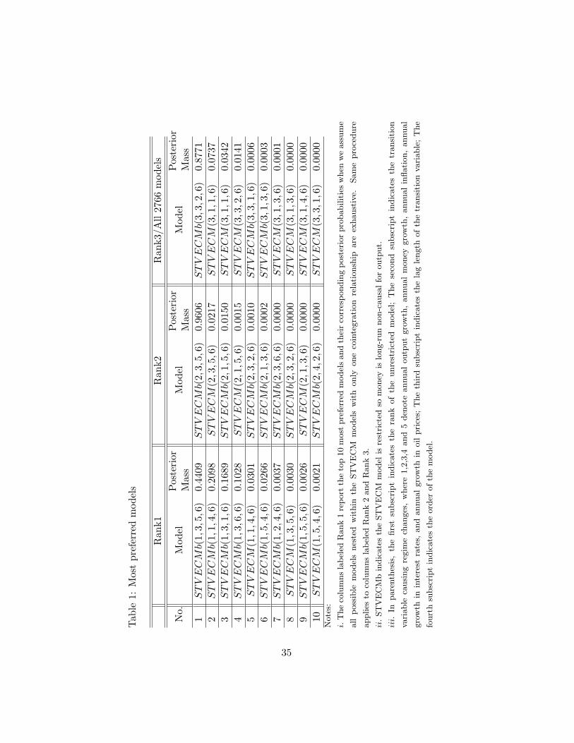
Assuming models nested within STVECMs with the same number of
cointegration ranks (from 1 to 3) to be exhaustive, we reports the top 10
models with the highest posterior model probabilities in table 1. Note that
the top 10 models of all the 2766 models are exactly the same as the top
10 models nested in the STVECM models with three cointegration rela-
tionships, for nonlinear models of rank 3 get nearly 100% of the posterior
mass among all the 2766 models. Table 1 reinforces the substantial support
for money long-run non-causality models. It is worth noting that the most
preferred models for all cases are nonlinear money long-run non-causality
models. Another interesting finding is that there is no pronounced model
uncertainty if we focus on all the 2766 possible models or a subset of mod-
els nested within the unrestricted STVECM models with 2 or 3 stochastic
trends. Yet, more evidence of model uncertainty emerges if we pre-impose
the cointegration rank of the unrestricted models to be 1. Finally, note
that the most preferred model among all the possible 2766 models is the
restricted money long-run non-causality STVECM of rank 3, order 6, and
with lagged 2 inflation rates as the transition indicator.
Overall, we find little support for models indicating money is not Granger-
causal for output. The posterior mass for all models (linear types of VAR,
VECM models and nonlinear types of STVAR, STVECM models) with zero
restrictions on the lagged money in the equations for output, price and
interest rates is nearly negligible. Furthermore, observing that the total13The model comparison results for models nested in each of the 90 unrestricted
STVECM models are available upon request.
21
posterior model probability associated with the unrestricted STVECMs and
the restricted money long-run non-causality STVECMs is almost 100%, we
proclaim that money nonlinearly Granger-causes output, which is in accord
with the in-sample evidence in Rothman, van Dijk and Frances (2001).
Given the substantial support for nonlinear models, it is interesting to
examine which transition variable plays a more important role in triggering
regime changes. Examining all the possible nonlinear models, we find that
lagged annual inflation rates consistently predominate over other candidate
transition variables in driving regime changes. All together, nonlinear mod-
els with lagged inflation rates as transition variables receive 89.17% of the
posterior mass. The next important triggers for regime changes are lagged
annual output growth rates. Note that nonlinear models with regime shift-
ing governed by the lagged annual output growth rates account for 10.83%
of the posterior mass. Last, compared with lagged inflation and output
growth, lagged changes in money, interest rates and oil prices play trivia
roles in triggering regime changes.
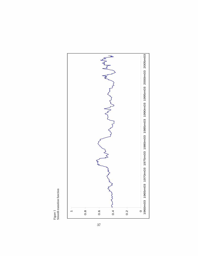
To highlight the nonlinear feature of the interrelationship among money,
output, prices and interest rates, in figure 1 we plot the values of the smooth
transition function over time for the most preferred model chosen from all the
2766 candidate models.14 Observe that although the plot is quite volatile,
the values of the transition function are almost always bounded by 0.4 and
0.6 throughout the time. This result implies that the regime changes in
the postwar US money-output relationship are quite modest, which is in
line with the findings of Primiceri (2005) and Sargent, Williams and Zha14The whole set of the time profiles of the transition functions are available upon request.
22
(2006). However, given the compelling support for nonlinear models over
linear models, it is worth stressing that we find it improper to model the
post-war US money-output relationship in linear models.
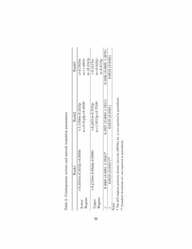
Table 2 contains the estimates of the cointegration vectors and transi-
tion parameters for the most preferred models nested in the unrestricted
STVECM models of rank 1, 2, 3, respectively. Recall that the most pre-
ferred model among the whole set of 2766 candidate models is exactly the
same most preferred model selected from all the possible models nested in
the unrestricted STVECM models of rank 3.
To aid in interpretation, in table 2, we normalize the cointegration vec-
tors on output and money, respectively. Assuming that the cointegration
rank is 1, we find the parameters for output, money and price levels appear
to have reasonable economic interpretations. For example, inflation brings
about (nominal) higher output level. Yet, it is not so straightforward to
explain why effects of interest rates are quite different between the lower
and upper regimes. Focusing on the model with 2 cointegration relation-
ships, we find that in each regimes, the first cointegrating vectors can be
explained as the (log) quasi-velocity of money as defined in Rothman, van
Dijk and Frances (2001), while it is hard to find an economic theory to ex-
plain the second long-run equilibrium relationship. For the most preferred
model among all the possible 2766 models (or the most preferred model
among all the models nested in STVECMs of rank 3), we find it even more
difficult to find a theory-based explanation for the long-run stationery in-
terrelationships. Yet, it is clear that there are enormous differences in the
cointegration vectors between the upper and lower regimes.
23
The estimated values of the smoothing parameter γ presented in table 2
are relatively small. With the speed of the transition determined by γ, small
value of γ indicates that the transition between regimes is rather smooth. As
to the estimated value of c, recall that for all cases, the transition variable
is the lagged inflation rates. In our sample, the mean of inflation rates is
0.0352. Given the threshold c is greater than 0.05 for each cases, it is seen
that the upper regimes only become active when the transition variable is
very large.
Finally, it is illuminating to look into the model comparison results in the
linear framework. Assuming the 66 linear models are exhaustive, we find
that the unrestricted linear VECM of rank 3 and order 6 receives nearly
100% of the posterior mass. Thus, models denoting long-run money non-
causality are no longer supported in the linear frameworks. Furthermore, we
find unrestricted VECM of order 6 dominates money long-run non-causality
models when we pre-specify the rank of the cointegration space to be 1 or
2. Nevethless, these results prove that ignoring nonlinear effects can lead to
quite misleading conclusions, such as money is long-run causal for output.
3.2 Impulse Response Analysis
To shed further light on the causal effects from money to output, we ana-
lyze the impulse responses of output given a shock to money. The nonlinear
STVECM allows for asymmetries in the behaviour of the money-output
linkages. In this study, we are interested in two types of asymmetric effects.
First, whether positive and negative shocks to money have unbalanced ef-
24
fects on real output. Second, whether big and small money shocks have
disproportionate effects.
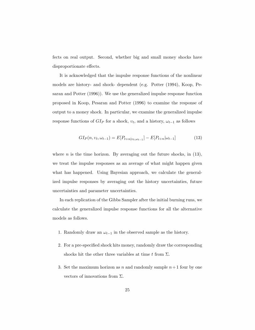
It is acknowledged that the impulse response functions of the nonlinear
models are history- and shock- dependent (e.g. Potter (1994), Koop, Pe-
saran and Potter (1996)). We use the generalized impulse response function
proposed in Koop, Pesaran and Potter (1996) to examine the response of
output to a money shock. In particular, we examine the generalized impulse
response functions of GIP for a shock, υt, and a history, ωt−1 as follows
GIP (n, υt, ωt−1) = E[Pt+n|υt,ωt−1]− E[Pt+n|ωt−1] (13)
where n is the time horizon. By averaging out the future shocks, in (13),
we treat the impulse responses as an average of what might happen given
what has happened. Using Bayesian approach, we calculate the general-
ized impulse responses by averaging out the history uncertainties, future
uncertainties and parameter uncertainties.
In each replication of the Gibbs Sampler after the initial burning runs, we
calculate the generalized impulse response functions for all the alternative
models as follows.
1. Randomly draw an ωt−1 in the observed sample as the history.
2. For a pre-specified shock hits money, randomly draw the corresponding
shocks hit the other three variables at time t from Σ.
3. Set the maximum horizon as n and randomly sample n+1 four by one
vectors of innovations from Σ.
25
4. Calculate the expected realizations of output using the shocks calcu-
lated in step 2 and the last n innovations in step 3.
5. Calculate the shock-independent expected realizations of output using
all the n+ 1 innovations in step 3.
6. Take the difference of the results from step 4 and step 5 to generate
the impulse responses of output for the current draw.
At the end of the Gibbs sampling scheme, we derive the generalized
impulse response functions for each possible model by integrating out all
the parameter uncertainties. Note that if there is a great deal of model
uncertainty, we can also average across models to derive the impacts of
money on output weighting by the posterior model probabilities.
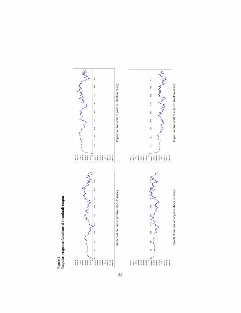
We set the magnitudes of the initial shocks amounting to ±1 and ±2
times the standard deviation of monthly money growth rates, namely ±1
unit and ±2 units of shocks. The time horizon of the impulse responses is
set as 600 months (50 years). Given the large number of models and four
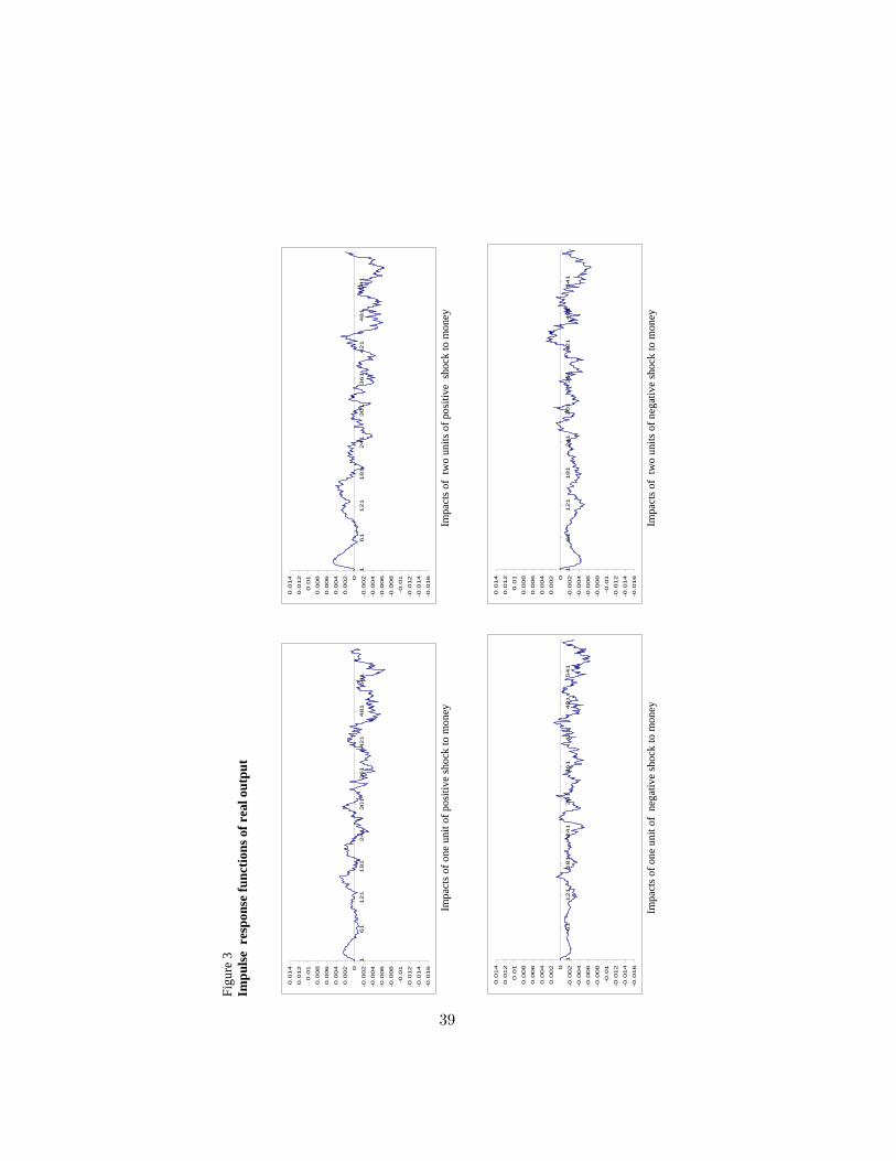
different shocks, we only present the impulse response functions for the most
preferred model among all the 2766 models in figures 2-3. For comparison,
both the impulse response functions of output (nominal output) and real
output are provided. The following observations are noteworthy in figures
2-3.
1. Positive and negative money shocks of the same magnitude appear
to have asymmetric affects on both nominal output and real output.
Observe that the time path of the impulse responses to positive shocks
26
never mirror that of the impulse responses to negative shocks.
2. Impacts on both nominal output and real output appear to vary dis-
proportionately with the size of the shock to money.
3. Impacts on nominal output appear to steadily increase in the same
direction of the initial shocks in the first 10 years. After that, the
impact responses become more volatile.
4. Compared with the responses of nominal output, the impact responses
of real output to a money shock are rather volatile. More strikingly,
the accumulated effect on real output appear to be negative in the
next 50 years after a shock to money, regardless of the size and sign
of the shock.
4 Conclusion
This paper investigates the causal effects from money to output using post-
war US data. We develop a Bayesian approach to catch the interrelationship
among money, output, prices and interest rates in a STVECM model. Dif-
ferent from similar nonlinear modeling method in the literature, we jointly
estimate the cointegration relationship and nonlinear effects in a single step
without pre-imposing any theory based restrictions.
Our model comparison results indicate that the postwar US money-
output relationship is nonlinear. Yet, we find that the transition between
regimes is rather smooth, and it is improper to use any abrupt transition
framework to model the money-output linkage. Through model compari-
27
son, we find substantial evidence in favor of money long-run non-causality
for output. In addition, we find little evidence against Granger causality
from money to output. More precisely, our result strongly support that
money nonlinearly Granger-causes output during the postwar period in the
US.
Our impulse response analysis sheds further light on the nonlinear causal
effects from money to output. An important finding that leaps out is that
although a positive money shock can increase nominal output, we have to
be cautious in using money as a policy instrument, for it appears that a
shock to money will have negative accumulative effects on real output over
the next fifty years, regardless of the size and sign of the shock.
References
[1] Ambler, S. (1989), Does Money Matter in Canada? Evidence from aVector Error Correction Model, The Review of Economics and Statis-tics, 71(4), 651-58.
[2] Barro, R. J. (1989), Interest-rate targeting, Journal of Monetary Eco-nomics 23(1), 3-30.
[3] Bartlett, M, S. (1957), A comment on D. V. Lindley’s statistical para-dox, Biometrika, 44, 533-34.
[4] Bauwens, L., M. Lubrano and J-F. Richard (1999), Bayesian inferencein dynamic econometric models, Oxford University Press: New York.
[5] Chib, S. and E. Greenberg (1995), Understanding the Metropolis-Hastings algorithm, The American Statistician 49(4), 327-35.
28
[6] Clarida, R., J. Galı and M. Gertler (2000), Monetary Policy Rulesand Macroeconomic Stability: Evidence and Some Theory, QuarterlyJournal of Economics, 115(1), 147-80.
[7] Coe, P. J. and J. M. Nason (2004), Long-run monetary neutrality andlong-horizon regressions, Journal of Applied Econometrics, 19(3), 355-73.
[8] Davies, R. B. (1977), Hypothesis testing when a nuisance parameter ispresent only under the alternative. Biometrika 74, 33-43.
[9] Duca, J. V. and D. D. VanHoose (2004), Recent Developments in Un-derstanding the Demand for Money, Journal of Economics and Busi-ness, 56, 247-72.
[10] Escribano, A. (2004) Nonlinear Error Correction: The Case of MoneyDemand in the United Kingdom 1878-2000, Macroeconomic Dynamics,8(1), 76-116.
[11] Friedman, B. M and K. N. Kuttner (1992), Money, Income, Prices, andInterest Rates, American Economic Review, 82(3), 472-92.
[12] Gefang, D. and R. W. Strachan (2007), Asymmetric Impacts of Inter-national Business Cycles on the UK - a Bayesian LSTVAR Approach,15th Annual Symposium of the Society for Nonlinear Dynamics andEconometrics, Paris.
[13] Geweke, J. (1992), Evaluating the accuracy of sampling-based ap-proaches to the calculation of posterior moments, in Bernodo, J.,Berger, J., Dawid, A. and Smith, A. (eds.) Bayesian Statistics, 4, 641-49, Oxford: Clarendon Press.
[14] Granger, C. and J-L. Lin (1995), Causality in the Long Run, Econo-metric Theory, 11(3), 530-36.
[15] Granger, C. and T. Terasvirta, (1993), Modelling Nonlinear EconomicRelationships, Oxford University Press: New York.
29
[16] Hall, S. G. and A. Milne (1994) The Relevance of P-Star Analysis toUK Monetary Policy, Economic Journal, 104(424), 597-604.
[17] Hall, S.G. and M. R. Wickens (1993), Causality in Integrated Systems,D.P. no. 27C93, Centre for Economic Forecasting, London BusinessSchool.
[18] Haug, A. A. and J. Tam (2007), A Closer Look at Long-Run U.S. MoneyDemand: Linear or Nonlinear Error-Correction With M0, M1, or M2?Economic Inquiry, 45(2), 363-76.
[19] Hill, J. B. (2007), Efficient tests of long-run causation in trivariate VARprocesses with a rolling window study of the money-income relationship,Journal of Applied Econometrics, 22(4), 747-65.
[20] James, A. T. (1954), Normal multivariate analysis and the orthogonalgroup, Analysis of Mathematical Statistics, 25, 40-75.
[21] Kapetanios, G., Y. Shin and A. Snell (2006), Testing for cointegrationin nonlinear smooth transition error correction models, EconometricTheory, 22, 279-303.
[22] King, R. G. and M. W. Watson (1997), Testing long-run neutrality,Economic Quarterly, Federal Reserve Bank of Richmond, 83, 69-101.
[23] Koop, G., R. Leon-Gonzalez and R. W. Strachan (2005), Efficient Pos-terior Simulation for Cointegrated Models with Priors On the Cointe-gration Space, Discussion Papers in Economics 05/13, Department ofEconomics, University of Leicester, revised Apr 2006.
[24] Koop, G., R. Leon-Gonzalez and R. W. Strachan (2006), Bayesian in-ference in a cointegration panel data model, Discussion Papers in Eco-nomics 06/2, Department of Economics, University of Leicester.
[25] Koop, G., M. H. Pesaran and S. M. Potter (1996), Impulse ResponseAnalysis in Nonlinear Multivariate Models, Journal of Econometrics,74, 491-99.
30
[26] Koop, G. and S. M. Potter (1999a), Bayes factors and nonlinearity:Evidence from economic time series, Journal of Econometrics, 88, 251-81.
[27] Koop, G. and S. M. Potter (1999b), Dynamic Asymmetries in US Un-employment, Journal of Business and Economic Statistics, 17, 298-313.
[28] Koop, G., R. W. Strachan, H. van Dijk and M. Villani (2006), BayesianApproaches to Cointegration, in T. Mills and K. Patterson (eds) ThePalgrave Handbook of Econometrics, Volume 1: Theoretical Economet-rics, Palgrave-Macmillan: Basingstoke.
[29] Leeper, E. M. and T. Zha (2003), Modest policy interventions, Journalof Monetary Economics, 50(8), 1673-1700.
[30] Leamer, E. E. (1978), Specification Searches, John Wiley, New York.
[31] LeSage, J. (1999), Applied econometrics using MATLAB.http://www.spatialeconometrics.com/.
[32] Lubrano, M. (1999a), Bayesian Analysis of Nonlinear Time Series Mod-els with a Threshold, In: Nonlinear Econometric Modelling, CambridgeUniversity Press, Cambridge.
[33] Lubrano, M. (1999b), Smooth Transition GARCH Models: A BayesianPerspective. Universite Aix-Marseille III G.R.E.Q.A.M. 99a49.
[34] Lutkepohl, H., T. Terasvirta and J. Wolters (1999), Investigating Sta-bility and Linearity of a German M1 Money Demand Function, Journalof Applied Econometrics, 14(5), 511-25.
[35] Meltzer, A. H. (2001), The Transmission Process, in: Deutsche Bun-desbank (Hrsg.), The Monetary Transmission Process - Recent Devel-opments and Lessons for Europe, Basingstoke, Palgrave, 112-30.
[36] Nelson, E. (2002), Direct effects of base money on aggregate demand:theory and evidence, Journal of Monetary Economics, 49(4), 687-708.
31
[37] Nelson, E. (2003), The future of monetary aggregates in monetary pol-icy analysis, Journal of Monetary Economics, 50(5), 1029-59
[38] Ni, S. X. and D. Sun (2003), Noninformative Priors and FrequentistRisks of Bayesian Estimators of Vector-Autoregressive Models, Journalof Econometrics, 115, 159-97.
[39] O’Hagan, A. (1995), Fractional Bayes factors for model comparison,Journal of the Royal Statistical Society, B 57, 99-138.
[40] Potter, S. (1994), Nonlinear impulse response functions, Department ofEconomics working paper (University of California, Los Angeles, CA).
[41] Primiceri, G. (2005), Why Inflation Rose and Fell: Policymakers’ Beliefsand US Postwar Stabilization Policy, NBER Working Papers 11147.
[42] Ritter, C. and M. A. Tanner (1992), Facilitating the Gibbs Sampler:The Gibbs Stopper and the Griddy-Gibbs Sampler, Journal of theAmerican Statistical Association, 87, 861-68.
[43] Rothman, P., D. van Dijk and P. H. Franses (2001), Multivariate StarAnalysis of Money-Output Relationship, Macroeconomic Dynamics,Cambridge University Press, 5(4), 506-32.
[44] Sargent, T., N. Williams and T. Zha (2006), Shocks and GovernmentBeliefs: The Rise and Fall of American Inflation, American EconomicReview, 96(4), 1193-1224.
[45] Seo, B. (2004), Testing for nonlinear adjustment in smooth transitionvector error correction models, Econometric Society, Far Eastern Meet-ings.
[46] Seo, M. (2006), Bootstrap testing for the null of no cointegration in athreshold vector error correction model, Journal of Econometrics, 143,129-50.
[47] Sims, C. (1972), Money, Income and Causality, American EconomicReview, 62, 540-52.
32
[48] Sims, C. (1980), Macroeconomics and Reality, Econometrica, 48, 1-48.
[49] Sims, C. A. and T. Zha (2006), Were There Regime Switches in U.S.Monetary Policy? American Economic Review, 96(1), 54-81.
[50] Stock, J. H. and M. W. Watson (1989), Interpreting the Evidence onMoney-Income Causality, Journal of Econometrics, 40, 161-81.
[51] Strachan, R. W. (2003), Valid bayesian estimation of the cointegratingerror correction model, Journal of Business and Economic Statistics,21(1), 185-95.
[52] Strachan, R. W. and B. Inder (2004), Bayesian analysis of the errorcorrection model, Journal of Econometrics, 123, 307-25.
[53] Strachan, R. W. and H. K. van Dijk (2004), Bayesian model selectionwith an uninformative prior, Keele Economics Research Papers KERP2004/01, Centre for Economic Research, Keele University.
[54] Strachan, R. W. and H. K. van Dijk (2006), Model Uncertainty andBayesian Model Averaging in Vector Autoregressive Processes, Discus-sion Papers in Economics 06/5, Department of Economics, Universityof Leicester.
[55] Swanson, N. R. (1998) Money and output viewed through a rollingwindow, Journal of Monetary Economics, 41(3), 455-74.
[56] Taylor, J. B. (1993), Discretion versus policy rules in practice, Carnegie-Rochester Conference Series on Public Policy, 39, 195 - 214.
[57] Taylor, J.B. (Ed.) (1999), Monetary Policy Rules. University of ChicagoPress, Chicago.
[58] Terasvirta, T. (1994), Specification, estimation and evaluation ofsmooth transition autoregressive models, Journal of the American Sta-tistical Association , 89(425), 208-18.
[59] Terasvirta, T. and A-C. Eliasson (2001), Non-linear error correctionand the UK demand for broad money, 1878-1993, Journal of AppliedEconometrics, 16(3), 277-88.
33
[60] Tong, H. (1983), Threshold Models in Non-linear Time Series Analysis,Springer-Verlag, New York.
[61] Villani, M. (2005), Bayesian reference analysis of cointegration, Econo-metric Theory, 21, 326-57.
[62] Wang, P. and Y. Wen (2005), Endogenous money or stickyprices?comment on monetary non-neutrality and inflation dynamics,Journal of Economic Dynamics and Control, 29, 1361-83.
[63] Weise, C. L. (1999), The Asymmetric Effects of Monetary Policy: ANonlinear Vector Autoregression Approach, Journal of Money Creditand Banking, 31, 85-108.
[64] Zellner, A. (1971), An introduction to Bayesian inference in economet-rics, John Wiley and Sons: New York.
34
Tab
le1:
Mos
tpr
efer
red
mod
els
Ran
k1R
ank2
Ran
k3/A
ll27
66m
odel
s
No.
Mod
elPos
teri
orM
ass
Mod
elPos
teri
orM
ass
Mod
elPos
teri
orM
ass
1STVECMb(
1,3,
5,6)
0.44
09STVECMb(
2,3,
5,6)
0.96
06STVECMb(
3,3,
2,6)
0.87
712
STVECMb(
1,1,
4,6)
0.20
98STVECM
(2,3,5,6
)0.
0217
STVECM
(3,1,1,6
)0.
0737
3STVECMb(
1,3,
1,6)
0.16
89STVECMb(
2,1,
5,6)
0.01
50STVECM
(3,1,1,6
)0.
0342
4STVECMb(
1,3,
6,6)
0.10
28STVECM
(2,1,5,6
)0.
0015
STVECM
(3,3,2,6
)0.
0141
5STVECM
(1,1,4,6
)0.
0301
STVECMb(
2,3,
2,6)
0.00
10STVECMb(
3,3,
1,6)
0.00
066
STVECMb(
1,5,
4,6)
0.02
66STVECMb(
2,1,
3,6)
0.00
02STVECMb(
3,1,
3,6)
0.00
037
STVECMb(
1,2,
4,6)
0.00
37STVECMb(
2,3,
6,6)
0.00
00STVECM
(3,1,3,6
)0.
0001
8STVECM
(1,3,5,6
)0.
0030
STVECMb(
2,3,
2,6)
0.00
00STVECM
(3,1,3,6
)0.
0000
9STVECMb(
1,5,
5,6)
0.00
26STVECM
(2,1,3,6
)0.
0000
STVECM
(3,1,4,6
)0.
0000
10STVECM
(1,5,4,6
)0.
0021
STVECMb(
2,4,
2,6)
0.00
00STVECM
(3,3,1,6
)0.
0000
Note
s:
i.T
he
colu
mns
label
edR
ank
1re
port
the
top
10
most
pre
ferr
edm
odel
sand
thei
rco
rres
pondin
gpost
erio
rpro
babilit
ies
when
we
ass
um
e
all
poss
ible
model
snes
ted
wit
hin
the
ST
VE
CM
model
sw
ith
only
one
coin
tegra
tion
rela
tionsh
ipare
exhaust
ive.
Sam
epro
cedure
applies
toco
lum
ns
label
edR
ank
2and
Rank
3.
ii.ST
VE
CM
bin
dic
ate
sth
eST
VE
CM
model
isre
stri
cted
som
oney
islo
ng-r
un
non-c
ausa
lfo
routp
ut.
iii.
Inpare
nth
esis
,th
efirs
tsu
bsc
ript
indic
ate
sth
era
nk
of
the
unre
stri
cted
model
;T
he
seco
nd
subsc
ript
indic
ate
sth
etr
ansi
tion
vari
able
causi
ng
regim
ech
anges
,w
her
e1,2
,3,4
and
5den
ote
annual
outp
ut
gro
wth
,annual
money
gro
wth
,annual
inflati
on,
annual
gro
wth
inin
tere
stra
tes,
and
annualgro
wth
inoil
pri
ces;
The
thir
dsu
bsc
ript
indic
ate
sth
ela
gle
ngth
of
the
transi
tion
vari
able
;T
he
fourt
hsu
bsc
ript
indic
ate
sth
eord
erofth
em
odel
.
35
Tab
le2:
Coi
nteg
rati
onve
ctor
san
dsm
ooth
tran
siti
onpa
ram
eter
s
Ran
k1R
ank2
Ran
k3
Low
erR
egim
e
i-0.
2031
m-0
.285
5p+
0.09
50r
i-1.
1168
m-0
.255
5pi+
0.19
23m
m+
0.21
49p+
0.28
29r
m+
1.88
85r
m-1
0.53
41p
Upp
erR
egim
e
i-0.
4150
m-0
.694
0p-0
.098
6ri-0.
4831
m-0
.725
2pi-0.
1417
mm
+1.
0513
p+0.
7710
rm
+0.
8494
rm
-0.8
133p
γ0.
4068
(0.0
001
2.29
46)*
0.19
57(0
.000
21.
2811
)0.
1826
(0.0
000
1.26
78)
c0.
0518
(0.0
301)*
*0.
0519
(0.0
301)
0.05
13(0
.030
2)
Note
s:
*T
he
95%
hig
hes
tpost
erio
rden
sity
inte
rvals
(HP
DIs
)fo
rγs
are
report
edin
pare
nth
esis
.
**
Sta
ndard
dev
iati
ons
ofc
are
report
edin
pare
nth
esis
.
36
Figu
re 1
Sm
ooth
tran
sitio
n fu
nctio
n
0
0.2
0.4
0.6
0.81
1960m
03
1965m
03
1970m
03
1975m
03
1980m
03
1985m
03
1990m
03
1995m
03
2000m
03
2005m
03
37
Figu
re 2
Im
puls
e r
espo
nse
func
tions
of (
nom
inal
) out
put
-0.0
16
-0.0
14
-0.0
12
-0.0
1
-0.0
08
-0.0
06
-0.0
04
-0.0
020
0.0
02
0.0
04
0.0
06
0.0
08
0.0
1
0.0
12
0.0
14
161
121
181
241
301
361
421
481
541
Im
pact
s of o
ne u
nit o
f pos
itive
shoc
k to
mon
ey
-0.0
16
-0.0
14
-0.0
12
-0.0
1
-0.0
08
-0.0
06
-0.0
04
-0.0
020
0.0
02
0.0
04
0.0
06
0.0
08
0.0
1
0.0
12
0.0
14
161
121
181
241
301
361
421
481
541
Im
pact
s of
two
units
of p
ositi
ve s
hock
to m
oney
-0.0
16
-0.0
14
-0.0
12
-0.0
1
-0.0
08
-0.0
06
-0.0
04
-0.0
020
0.0
02
0.0
04
0.0
06
0.0
08
0.0
1
0.0
12
0.0
14
161
121
181
241
301
361
421
481
541
Im
pact
s of o
ne u
nit o
f ne
gativ
e sh
ock
to m
oney
-0.0
16
-0.0
14
-0.0
12
-0.0
1
-0.0
08
-0.0
06
-0.0
04
-0.0
020
0.0
02
0.0
04
0.0
06
0.0
08
0.0
1
0.0
12
0.0
14
161
121
181
241
301
361
421
481
541
Im
pact
s of
two
units
of n
egat
ive
shoc
k to
mon
ey
38
Figu
re 3
Im
puls
e r
espo
nse
func
tions
of r
eal o
utpu
t
-0.0
16
-0.0
14
-0.0
12
-0.0
1
-0.0
08
-0.0
06
-0.0
04
-0.0
020
0.0
02
0.0
04
0.0
06
0.0
08
0.0
1
0.0
12
0.0
14
161
121
181
241
301
361
421
481
541
Im
pact
s of o
ne u
nit o
f pos
itive
shoc
k to
mon
ey
-0.0
16
-0.0
14
-0.0
12
-0.0
1
-0.0
08
-0.0
06
-0.0
04
-0.0
020
0.0
02
0.0
04
0.0
06
0.0
08
0.0
1
0.0
12
0.0
14
161
121
181
241
301
361
421
481
541
Im
pact
s of
two
units
of p
ositi
ve s
hock
to m
oney
-0.0
16
-0.0
14
-0.0
12
-0.0
1
-0.0
08
-0.0
06
-0.0
04
-0.0
020
0.0
02
0.0
04
0.0
06
0.0
08
0.0
1
0.0
12
0.0
14
161
121
181
241
301
361
421
481
541
Im
pact
s of o
ne u
nit o
f ne
gativ
e sh
ock
to m
oney
-0.0
16
-0.0
14
-0.0
12
-0.0
1
-0.0
08
-0.0
06
-0.0
04
-0.0
020
0.0
02
0.0
04
0.0
06
0.0
08
0.0
1
0.0
12
0.0
14
161
121
181
241
301
361
421
481
541
Im
pact
s of
two
units
of n
egat
ive
shoc
k to
mon
ey
39