Embed Size (px)
Citation preview
TRANSPORT THEORIES OF HEAVY-ION REACTIONS
HANS A. WEIDENMI~ILLER
Max-Planck-lnstitut fiir Kernphysik, Heidelberg, W. Germany
CONTENTS
1. INTRODUCTION 49 2. PHYSICAL PICTURES AND THEORETICAL MODELS FOR DIC 51 3. MACROSCOPIC DESCRIPTioN OF DIC 58
3.1. Features of a macroscopic description ~2°7} 58 3.2. Fokker-Planck equations ~s s } 59 3.3. Master equations ~ss~ 63 3.4. Phenomenological analyses of DIC in terms of transport equations 66 3.5. Typical results of the analyses 70 3.6. Conclusion 87
4. VALIDITY OF TRANSPORT THEORIES, TIME SCALES, WEAK AND STRONG CoUPLING 88 4.1. Estimate of time scales 88 4.2. A statistical model 92
5. SURVEY OF THE THEORETICAL APPROACHES 97 5.1. The theory of Gross and coworkers ¢2°'9°'92'93'9"'9s'97) 99 5.2. The two-centre shell-model approach of Glas and Mosel ~s6"se~ 100 5.3 The proximity method of Swiatecki, Randrup et al. c34"}24"125"~ 7s.t79.2o2, 103 5.4. The "linear response" theory of Hofmann, Siemens eta/. ~1°3.}°'t.1°6"}°7,1 io.t i i .i 12.118.185} 106 5.5. Transport coefficients in strong coupling: the theory of N6renberg, Ayik
et al. (9'10'12'164'}65'167"168"194) 109
5.6 Transport equations for strong coupling: the approach of Agassi, Ko et al. t3-6'} t~,} 23.126,187.218-220} 112
6. OUTLOOK 117 REFERENCES 119 APPENDICES 123
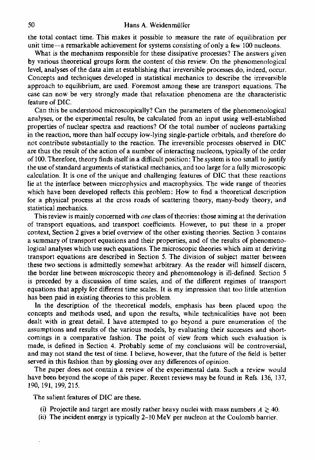
1. INTRODUCTION
Typ ica l con tac t t imes of two heavy ions in deeply inelast ic col l is ions (DIC) are of the o rde r 10 -21 s. This t ime is not much larger than the typical t ime of a d i rec t react ion, 10-22 s. Yet, d iss ipa t ive processes a n d equ i l ib ra t ion p h e n o m e n a tha t seem to involve all the ava i lab le phase space are typical for D I C : A subs tan t ia l f ract ion of the inc ident energy (several MeV per nuc leon at the C o u l o m b barr ie r ) is conver t ed into heat, and the two f ragments exchange neu t rons and p ro tons in a diffusion-l ike process. By jud ic ious ly choos ing the angle of obse rva t ion of the reac t ion produc ts , o r o ther p a r a m e t e r s of the react ion, the exper imenta l i s t can even ad jus t the degree of equ i l ib ra t ion or, in some sense,
49
50 Hans A. Weidenmfiller
the total contact time. This makes it possible to measure the rate of equilibration per unit time--a remarkable achievement for systems consisting of only a few 1130 nucleons.
What is the mechanism responsible for these dissipative processes? The answers given by various theoretical groups form the content of this review. On the phenomenological level, analyses of the data aim at establishing that irreversible processes do, indeed, occur. Concepts and techniques developed in statistical mechanics to describe the irreversible approach to equilibrium, are used. Foremost among these are transport equations. The case can now be very strongly made that relaxation phenomena are the characteristic feature of DIC.
Can this be understood microscopically? Can the parameters of the phenomenological analyses, or the experimental results, be calculated from an input using well-established properties of nuclear spectra and reactions? Of the total number of nucleons partaking in the reaction, more than half occupy low-lying single-particle orbitals, and therefore do not contribute substantially to the reaction. The irreversible processes observed in DIC are thus the result of the action of a number of interacting nucleons, typically of the order of 100. Therefore, theory finds itself in a difficult position: The system is too small to justify the use of standard arguments of statistical mechanics, and too large for a fully microscopic calculation. It is one of the unique and challenging features of DIC that these reactions lie at the interface between microphysics and macrophysics. The wide range of theories which have been developed reflects this problem: How to find a theoretical description for a physical process at the cross roads of scattering theory, many-body theory, and statistical mechanics.
This review is mainly concerned with o n e class of theories: those aiming at the derivation of transport equations, and transport coefficients. However, to put these in a proper context, Section 2 gives a brief overview of the other existing theories. Section 3 contains a summary of transport equations and their properties, and of the results of phenomeno- logical analyses which use such equations. The microscopic theories which aim at deriving transport equations are described in Section 5. The division of subject matter between these two sections is admittedly somewhat arbitrary. As the reader will himself discern, the border line between microscopic theory and phenomenoiogy is ill-defined. Section 5 is preceded by a discussion of time scales, and of the different regimes of transport equations that apply for different time scales. It is my impression that too little attention has been paid in existing theories to this problem.
In the description of the theoretical models, emphasis has been placed upon the concepts and methods used, and upon the results, while technicalities have not been dealt with in great detail. I have attempted to go beyond a pure enumeration of the assumptions and results of the various models, by evaluating their successes and short- comings in a comparative fashion. The point of view from which such evaluation is made, is defined in Section 4. Probably some of my conclusions will be controversial, and may not stand the test of time. I believe, however, that the future of the field is better served in this fashion than by glossing over any differences of opinion.
The paper does not contain a review of the experimental data. Such a review would have been beyond the scope of this paper. Recent reviews may be found in Refs. 136, 137, 190, 191, 199, 215.
The salient features of DIC are these.
(i) Projectile and target are mostly rather heavy nuclei with mass numbers A > 40. (ii) The incident energy is typically 2-10 MeV per nucleon at the Coulomb barrier.
Transport Theories of Heavy-Ion Reactions 51
(iii) A large fraction of this energy is converted into intrinsic excitation energy of either fragment, leading to energy losses of typically several 100 MeV.
(iv) The angular distribution is strongly non-isotropic with the characteristic properties of a peripheral fast reaction.
(v) Events with a large number (~. 20) of transferred nucleons are observed. The cross- sections depend smoothly on charge and mass transfer.
(vi) Up to 40-50 units of h of angular momentum of relative motion are converted into intrinsic spin of either fragment.
(vii) The total cross-section for deeply inelastic collisions increases with the masses of the colliding nuclei, and with bombarding energy. For heavy nuclei, typical values for the total DIC cross-sections are of the order of several barns.
(viii) The cross-sections are inclusive cross-sections: Only the kinetic energy, mass and atomic number of one fragment are usually observed. Since the excitation energies are high, the number of channels is very large, and therefore only averaged quantities are observed.
Of the theoretical reviews preceding this paper, I mention a general introduction to the theory of heavy-ion scattering, (~66) a survey of theories of DIC given at Caen by N6renberg.(167)
Although this article is not primarily didactic in purpose, and in spite of the lack of a survey of the experimental material in it, I have aimed at a pedagogical presentation of theoretical concepts. This has only b~n possible at the expense of brevity. In view of the considerable lack of familiarity of the nuclear physics community with irreversible processes, such an approach is hopefully justified.
The paper has evolved from a series of lectures given at the NATO summer school in Madison in 1978. (219) Both the lectures and this article were prepared while I had the privilege of visiting the Department of Theoretical Physics of the University of Oxford. Thanks are due to D. M. Brink for making this visit possible, to K. W. McVoy for inviting me to lecture in Madison, and to D. Wilkinson for suggesting that I write this review. I have profited from extensive correspondence with H. Hofmann in Munich. H. Kalinowski, W. N6renberg, D. Pelte, D. Saloner and G. Wolschin read preliminary versions of this article, and made valuable suggestions. Needless to say, the responsibility for all remaining errors is mine. I sincerely apologise to all those workers in the field whose work I overlooked, or misrepresented.
2. PHYSICAL PICTURES AND THEORETICAL MODELS FOR DIC
It is the purpose of this review to give an account of transport-theoretical approaches towards DIC. To see these approaches in their proper perspective, it is useful to recall the existence of other theoretical formulations which do not use the vehicle of transport theory, and to briefly review the landscape of theories and physical ideas used to understand the observed phenomena. It is the purpose of this section to provide such a review. Transport theory will then be so~n to be part of a whole spectrum of possible approaches. (7°)
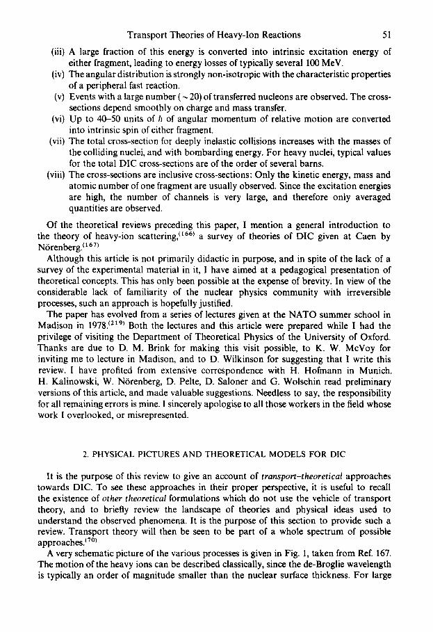
A very schematic picture of the various processes is given in Fig. l, taken from Ref. 167. The motion of the heavy ions can be described classically, since the de-Broglie wavelength is typically an order of magnitude smaller than the nuclear surface thickness. For large
52 Hans A. Weidenmiiller
elastic scstts¢ing direct r eec t~
grazi~ ¢ o l l i s i o n ~ f '1~B" , ~ ~ ", cornpo~nd-nuclsu$
__~_bll.r _ _ _ _ , ' ~ . _ x'x) " formatKm _
clo~ collisions ',f--~R~ j ,
" ' ~ deepl-'-'--y inel-"~stie collision distant collision
elastic (Rutherford) scattering Cou4omb excitation
Fig. 1. Distant, grazing and close collisions in the classical picture of heavy-ion scattering (taken from Ref. 167).
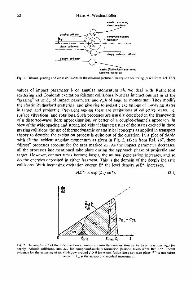
values of impact parameter b or angular momentum Eh, we deal with Rutherford scattering and Coulomb excitation (distant collisions). Nuclear interactions set in at the "grazing" value bgr of impact parameter, and E,rh of angular momentum. They modify the elastic Rutherford scattering, and give rise to inelastic excitations of low-lying states in target and projectile. Prevalent among these are excitations of collective states, i.e. surface vibrations, and rotations. Such processes are usually described in the framework of a distorted-wave Born approximation, or better of a coupled-channels approach. In view of the wide spacing and strong individual characteristics of the states excited in these grazing collisions, the use of thermodynamic or statistical concepts as applied in transport theory to describe the excitation process is quite out of the question. In a plot of da/dg with l'h the incident angular momentum as given in Fig. 2, taken from Ref. 167, these "direct" processes account for the area marked 00. As the impact parameter decreases, all the processes just mentioned take place during the approach phase of projectile and target. However, contact times become larger, the mutual penetration increases, and so do the energies deposited in either fragment. This is the domain of the deeply inelastic collisions. With increasing excitation energy E* the level density p(E*) increases,
p(E*) ~ exp (2~/aE*), (2.1)
do" / d"~ / / " f f
o"EL + o"CE
=_._ 0 ~¢rit ~max ~gr
Fig. 2. Decomposition of the total reaction cross-section into the cross-section ao for direct reactions, <rmc for deeply inelastic collisions, and <rcN for compound-nuc]eus formation (fusion), taken from Ref. 167. Recent evidence for the existence of an g-window around g > 0 for which fusion does not take place ~sT) is not taken
into account, koo is the asymptotic incident momentum.
Transport Theories of Heavy-Ion Reactions 53
where the level density parameter a .has typical values a = AJ(10 MeV) with A~, i = 1, 2 the mass numbers of the fragments. The ever more narrowly spaced levels lose their individual characteristics, and so do the excitation processes that feed them. For these deeply inelastic collisions, a statistical treatment is then probably adequate after the approach phase, and is definitely to be preferred over a coupled-channels approach which becomes prohibitive. This is the domain where transport equations are best put to use. There is evidence that at the end of a deeply inelastic collision, and for sufficiently small values of the impact parameter, a lump of hot nuclear matter is formed. This deformed, non-spherical lump rotates for some fraction of a complete revolution and eventually either fissions, being broken apart by Coulomb and centrifugal forces after it has elongated sufficiently, or fuses. A fused system can, of course, also undergo fission. The distinction between breakup following deformation in deeply inelastic collisions, and fission of a fused system, is usually made via the angular distribution or, less unambiguously, via the mass distribution of the reaction products, see, however, Ref. 101.
The curves of Fig. 2 are schematic in several respects. Firstly, as remarked in the figure caption, there is some evidence that for light systems and very small values of the incident angular momentum hg, fusion may not take place. ~t57~ Secondly, there is growing evidence that, among the remaining g-values, none are exclusively reserved for direct reactions.~ga.17 a.183~ It appears that even at the grazing angular momentum, the fraction of (da/dg) that goes into fusion does not vanish. A theoretical argument in this context may be found in Ref. 105. Finally, it must be borne in mind that trotc/trc• becomes very small (large) for light (heavy) systems and small (large) bombarding energies, respectively.
The theoretical approaches used to describe these phenomena reflect the wide range of processes mentioned, and fall mainly into three categories: (i) The use of surface vibrations as the agents through which energy is transported from relative motion into intrinsic excitation ~(47-49,51,52) (ii) the use of time-dependent Hartree--Fock calculations to account for the main features observed in DIC ;tlT,7~.121.15s,~77~ (iii) the use of transport equations as described in later sections of this review.
The approach pursued by Broglia, Dasso, Winther, and collaborators t47-49'51'52~ emphasizes the role of surface vibrations in each fragment, excited by the presence of the other, for the transfer of energy and angular momentum. These modes are taken to be the RPA modes of the two independent, free fragments, calculated from a suitable nuclear model. The modes are described as damped harmonic oscillations. The damping is due to energy flowing from the collective excitation into other intrinsic degrees of freedom. The driving force is given by the shape-dependent Coulomb force (Coulomb excitation) and, more importantly, by the shape-dependent proximity force, calculated from the proximity potential between two heavy ions (Ref. 35, see also Section 3). The nuclear shapes are given, at each instant of time, in terms of the surface vibrations which are treated as classical harmonic oscillations. This approach extends in a simple, powerful way the essentials of a coupled-channels calculation to the domain of smaller impact parameters. The approach has recently been generalised, and mass transfer between the two heavy ions has been included, t51'52~ This is done by using the average rate of mass transfer as calculated in the proximity models (Ref. 34 and Section 5), and adding the corresponding friction forces to the equations for relative motion. Mass transfer is thus treated as a proper transport phenomenon, i.e. as incoherent, while inelastic excitation is described as a coherent process. The widths of the observed energy spectra and angular distributions have accordingly two origins: a statistical widening (diffusion process) connected with the energy and angular momentum transport through mass transfer, and a quantum spread
54 Hans A. Weidenmiiller
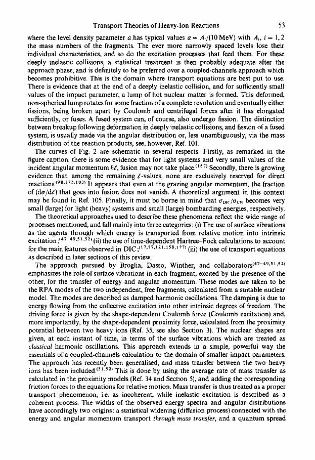
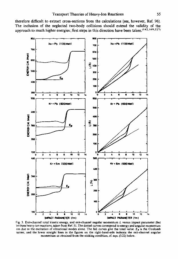
due to the quantum fluctuations of the number of bosons excited in each vibrational mode. Mass transfer and vibrations contribute about equally to the loss of energy and angular momentum/TM One particular strong point of this approach is that the coupling of the vibrational modes to relative motion fulfils the sum rules by construction, whereas friction coefficients in the phenomenological approaches of Section 3 are often just fitted to the data. The results of the calculations (see Fig. 3), taken from Ref. 51, show encouraging agreement with the data, and with results of calculations using time-dependent Hartree--Fock theory. Nevertheless, some questions remain open: (i) How justified is the use of vibrational modes of the separated fragments as the only important collective modes of the dynamics of the joint system? A qualitative answer is that the density overlap is small in DIC (only a few per cent of the total density), and that the vibrational periods are substantially larger than the duration time of the collision. (ii) One should expect that with increasing excitation energy of each fragment, the surface vibrations become more and more mixed with the other modes of intrinsic excitation. As a result, the coherence of the process should be lost, and the resulting incoherence should give rise to equations of transport type, without violation of the sum rules. This question has not been fully answered yet, cf. Refs. 126, 210. (iii) It is not clear yet whether the model can account for the finer details of the cross-sections, i.e. double and triple differential cross-sections versus energy transfer, angle, and mass transfer (cf. Section 3)/18°) (iv) A detailed micro- scopicjustification for the forces which damp the vibrations has apparently not yet been given.
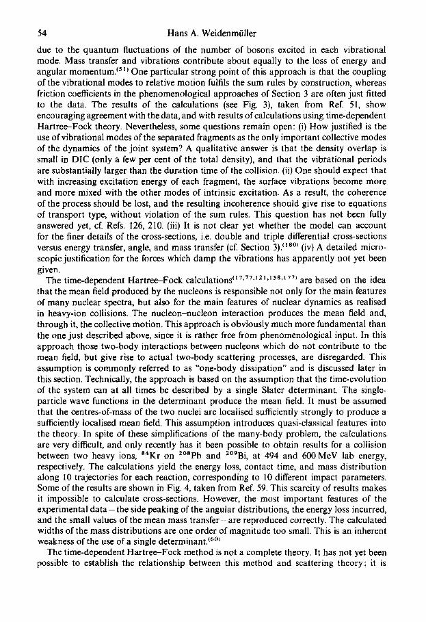
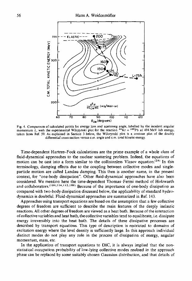
The time-dependent Hartree-Fock calculations ~ I 7,77, i 210158.177) are based on the idea that the mean field produced by the nucleons is responsible not only for the main features of many nuclear spectra, but also for the main features of nuclear dynamics as realised in heavy-ion collisions. The nucleon-nucleon interaction produces the mean field and, through it, the collective motion. This approach is obviously much more fundamental than the one just described above, since it is rather free from phenomenological input. In this approach those two-body interactions between nucleons which do not contribute to the mean field, but give rise to actual two-body scattering processes, are disregarded. This assumption is commonly referred to as "one-body dissipation" and is discussed later in this section. Technically, the approach is based on the assumption that the time-evolution of the system can at all times be described by a single Slater determinant. The single- particle wave functions in the determinant produce the mean field. It must be assumed that the centres-of-mass of the two nuclei are localised sufficiently strongly to produce a sufficiently localised mean field. This assumption introduces quasi-classical features into the theory. In spite of these simplifications of the many-body problem, the calculations are very difficult, and only recently has it been possible to obtain results for a collision between two heavy ions, 84Kr on 2°Spb and 2°9Bi, at 494 and 600 MeV lab energy, respectively. The calculations yield the energy loss, contact time, and mass distribution along I0 trajectories for each reaction, corresponding to 10 different impact parameters. Some of the results are shown in Fig. 4, taken from Ref. 59. This scarcity of results makes it impossible to calculate cross-sections. However, the most important features of the experimental data - t h e side peaking of the angular distributions, the energy loss incurred, and the small values of the mean mass transfer--are reproduced correctly. The calculated widths of the mass distributions are one order of magnitude too small. This is an inherent weakness of the use of a single determinant. <6°)
The time-dependent Hartree-Fock method is not a complete theory. It has not yet been possible to establish the relationship between this method and scattering theory; it is
Transport Theories of Heavy-Ion Reactions 55
therefore difficult to extract cross-sections from the calculations (see, however, Ref. 96). The inclusion of the neglected two-body collisions should extend the validity of the approach to much higher energies; first steps in this direction have been taken. (14z,t69,227)
800 i ! | I ! ~ v i 1 , i ; /
Xe * Pb (1130 MeV) | Xe • PI:) ( 1130 IqeV)
300 , ~ L ~ ~ , I o ~ , ° ° t " l ' ~ ' ' ' ' ' t ~. 6 o lo 12 l& o 2 & 8 II !o t2 l&
Kr'Pb (60014eV) [ 5001 Kr*Pt) (600kleV)
p
,oo ; I ; ; ~o ;, ," °o , . , , ,o ,, , ,
~o . . . . . . I "=1 . . . . . . ,,~.s,,, t~oo..Vl I ~ L ~ . s . q . o ~ )
i 11111 ' 0 o z • s e ~o ~z 1,- o z ,- s e m ~z ~.
DdPACT PARAMETER (fro) IMPACT PARAMETER (fro) Fig. 3. Exit-channel total kinetic energy, and exit-channel angular momentum L versus impact parameter (fm) br three heavy-ion reactions, taken from Ref. 5 I. The dotted curves correspond to energy and angular momentum oss due to the excitation of vibrational modes alone. The full curves give the total value. Em is the Coulomb )arrier, and the lower straight lines in the figures on the right-hand-side indicate the exit-channel angular
momentum as obtained from the sticking condition, cf. eqn. (3.22) below.
56 Hans A. WeidenmiJller
L I I I I I I
- - 3 5 6 - - - - ELASTIC---- "~200-- ~ 2.~ >
200 I 1
60 ;'o 8o 90 Ioo llo )zo Ocu (degrees)
Fig. 4. Comparison of calculated points for energy loss and scattering angle, labelled by the incident angular momentum L, with the experimental Wilczynski plot for the reaction S4Kr + 2°SPb at 494 MeV lab energy, taken from Ref. 59. As explained in Section 3 below, the Wilczynski plot is a contour plot of the doubly
differential cross-section versus c.m. angle and c.m. total kinetic energy.
Time-dependent Har t ree-Fock calculations are the prime example of a whole class of fluid-dynamical approaches to the nuclear scattering problem. Indeed, the equations of motion can be cast into a form similar to the collisionless Vlasov equation. (24) In this terminology, damping effects due to the coupling between collective modes and single- particle motion are called Landau damping. This then is another name, in the present context, for "one-body dissipation". Other fluid-dynamical approaches have also been considered. We mention here the time-dependent Thomas-Fermi method of Holzwarth and collaborators. (1 o9,114.1 ~s,1 a6) Because of the importance of one-body dissipation as compared with two-body dissipation discussed below, the applicability of standard hydro- dynamics is doubtful. Fluid-dynamical approaches are summarized in Ref. 143.
Approaches using transport equations are based on the assumption that a few collective degrees of freedom are sufficient to describe the main features of the deeply inelastic reactions. All other degrees of freedom are viewed as a heat bath. Because of the interaction of collective variables and heat bath, the collective variables tend to equilibrate, i.e. dissipate energy irreversibly into the heat bath. The details of these dissipative processes are described by transport equations. This type of description is restricted to domains of excitation energy where the level density is sufficiently large. In this approach individual distinct modes do not play any role in the process of dissipation of energy, angular momentum, mass, etc.
In the application of transport equations to DIC, it is always implied that the non- statistical occupation probability of low-lying collective modes realised in the approach phase can be replaced by some suitably chosen Gaussian distribution, and that details of
Transport Theories of Heavy-Ion Reactions 57
this probability distribution are not important for the later evolution. This question has not been fully investigated.
Common to all recent theoretical models is the emphasis on the "one-body dissipation" mechanism, and the neglect of "two-body dissipation". (34~ Generally speaking, this means that the coupling between the collective degrees of freedom and the single-particle degrees of freedom constitutes the most important vehicle of energy transfer and dissipative behaviour, and that the two-body collisions play no, or only a minor, role. This is a concept quite similar to the basic idea of time-dependent Hartree-Fock calculations. The justification derives from the sizeable mean free path ;t (~. > R, the nuclear radius) of nucleons of low energy (<20 MeV above the Fermi surface), see Sections 4 and 5. Specifically, one-body dissipation implies that in the region of space where the mass densities ofthe two fragments overlap, nucleons in one fragment are scattered inelastically by the potential well of the other (inelastic scattering), or penetrate into the volume of the other fragment (mass transfer). It is mainly these processes through which energy and angular momentum of relative motion are transferred into intrinsic degrees of freedom. The nucleons which partake in these reactions leave the overlap region before they collide with other nucleons. This picture has to be contrasted with the usual, two-body viscosity of hydrodynamics which is caused by two-body collisions, and which would lead to a local heating of the region where the densities overlap: s~'2t6'z17~ A more detailed discussion of one-body dissipation is given in Section 5.3.
The dissipation of energy in DIC may be thought of as being similar to the energy dissipation in fission: 2°6'2°~ This latter problem has received a considerable amount of at tent ion. (36"37''Ll'134,141,163'l~l'lss'lsg'192'lgs'196) There exist, however, appreciable dif- ferences: At the saddle point, the scissioning nucleus is cold (T ~ 0 for excitation energies up to the fission barrier); it gets partially heated on the descent from the saddle point to the scission configuration. In DIC, a considerable amount of energy (~20 MeV) is deposited into the fragments in the approach phase, before the onset of the regime of a transport description. Moreover, the relative velocity is high at the beginning of a DIC. Nonetheless, concepts evolved in the context of nuclear fission have also been applied to DIC, especially by Glas and Mosel: 8sl This will be reviewed in Section 5.2.
Among the three approaches described above, time-dependent Hartree-Fock calcu- lations are the most fundamental ones, and most directly related to the basic nucleon- nucleon force. While the relevant collective variables must be chosen in both the Broglia-Dasso--Winther approach, and in transport theory, Hartree-Fock calculations yield an (albeit implicit) knowledge of the collective variables relevant for the problem. The Broglia-Dasso-Winther approach is quite close in the basic physical assumptions made to transport theory. In particular, mass transfer is viewed as a transport phenomenon in both approaches, and the low-lying collective modes which describe nuclear deformation with long time scales are viewed as essential collective modes in both theories. The major difference in the two models concerns the role of the high-lying collective vibrations with excitation energies of ~ 10 MeV and more. In the Broglia-Dasso--Winther model, these vibrations act coherently, while in a transport description their strength is completely broken up and distributed over the intrinsic eigenstates of the system. As a consequence, fluctuations about the mean energy loss, mean angular momentum etc. are quantal in the Broglia-Dasso-Winther approach (save for those caused by mass transport), statistical in transport approaches. A choice between these models can probably only, if ever, be made by means of a detailed comparison of their predictions with the data.
Aside from the dynamical approaches just described, there exist formal procedures
58 Hans A. Weidenm/iller
which utilise statistical properties of the scattering matrix) 69'2091 These procedures establish a direct, though formal, link with compound-nucleus reactions on the one hand, and direct reactions on the other. In both procedures, a framework is established which has yet to be filled with dynamical detail. Strutinsky, in particular, emphasises the differences between the coherent features of the S-matrix dominating the near-grazing collisions, and the statistical features dominating the deeply inelastic ones. t2°91 He shows that simple parametrisations of the statistical S-matrix can reproduce many qualitative aspects of DIC. This is the merit of his approach. The parameters appearing in his theory are the essential "observables" of the process. It is to be hoped that in the future, this type of description can be used to reduce to their essentials the less transparent microscopic transport theories.
3. MACROSCOPIC DESCRIPTION OF DIC
3.1. Features of a macroscopic descriptio# 2°71
A macroscopic description of DIC is based on the idea that the gross features of a collision between two sizeable lumps of nuclear matter (both mass number Ai ~> 1) can be described in terms of a small number of variables. Classical equations of motion are used to describe the time evolution of these collective variables. Since equations of motion involve time derivatives of up to second order, three quantities must be specified for each equation: the conservative potential (including possibly coupling terms between different collective variables), the inertia parameter (mass, moment of inertia, etc.), and the friction force.
Obvious candidates for collective variables, and the ones most often used in practice, are: (i) the distance r between the centres-of-mass of the colliding ions; (ii) shape degrees of freedom describing the surfaces of the two ions, and of the composite system ; (iii) the distribution of mass and charge over the two ions, and in the composite system. For a near-grazing collision, this distribution can be specified in terms of the mass At and charge Z1 of fragment 1.
The hope that a macroscopic description be viable is based upon the inequalities Ai ~ 1, i = 1,2. For the variable r, these inequalities imply that even for fairly small velocities Iv I (typically Ivl = 0.1 c at the Coulomb barrier), the de-Broglie wave length is short (0.05 to 0.1 fm) compared to typical distances (0.5 to 1.0 fm) over which the nuclear potential changes. For the mass and charge distributions, a description in terms of surface parameters becom6s meaningful for A~ ,> 1 ("leptodermous systems"~2°7~).
The friction forces account in a global fashion for the coupling between the collective variables and the other degrees of freedom of the system. They describe the irreversible flow of energy and angular momentum from the collective motion into other modes of excitation. Except for their role as a "heat bath", and as providers of phase space, these non-collective modes are assumed not to affect the dynamics of a heavy-ion collision. Friction forces thus describe a partial equilibration process. If they act long enough, the system reaches thermal equilibrium and the available energy is shared equally among all the degrees of freedom.
This global treatment of the non-collective modes of excitation as some kind of heat bath obviously supposes that ~1°6'1 to~
Zeq u ~ "t'coll. (3.1)
Transport Theories of Heavy-Ion Reactions 59
Here, %qu is the time it takes the non-collective modes to reach internal equilibrium, while Zco, is the time over which the collective variable(s) change(s) significantly.
The simplest example of a macroscopic description is that of the equation of motion for the variable r. With r = {x~}, ~t = 1, 2, 3 and t the time, we have for a = I, 2, 3
/~,(t) + ~ ~(r)~(t )+ O-~-V dx~ (r) = 0. (3.2)
The conservative potential is V(r), # is the mass, and 3,~p(r) is the friction tensor. In the general form of eqn. (3.2), the friction contains "radial friction" (acting in the direction of r), "tangential friction" (acting ~rpendicularly to r and responsible for the loss of orbital angular momentum), and a cross-term.
From a phenomenological analysis of cross-section data with the help of eqn. (3.2), it is not possible to determine simultaneously p., V(r), and 7~p. At least some of these quantities and their dependence on r must be specified a priori. For this, one takes recourse to microscopic models. The potential V(r) is often determined from the liquid drop model,/~ is taken to be the reduced mass even when the nuclear densities overlap, and "/~B is written as the product of a friction constant (or a friction tensor) and a form factor, the latter being, for instance, given by the density overlap of the two fragments. The aim of a phenomenological analysis is then twofold: (i) to determine certain para- meters (the strength of radial and tangential friction, for instance), and (ii) to collect evidence for the presence of further collective variables not yet included in the description. If this process converges, it yields, via a fit of the cross-sections, a "complete" set of collective variables, and a suitable and successful parametrization of the associated potentials, inertia parameters, and friction forces. From the evidence presently available, it appears that the variables mentioned above-dis tance , shape, and mass and charge distr ibution--do form such a "complete" set.
In the context of heavy-ion physics, the success of such a procedure, and the existence of a limited number of collective variables, is not obvious a priori. The masses Ai are typically only two orders of magnitude larger than one, and the associated inertia parameters may be too small to guarantee the validity of the inequality (3.1). Even if the inequality (3.1) is satisfied for some collective variable, we cannot exclude a priori the existence of a whole chain of collective variables with ever decreasing characteristic times, rcotl, which continuously merge with the time scales characterising what we called the "non-collective modes of excitation". In this respect, the nuclear case is quite different from that of Brownian motion where the mass of the Brownian particle is many orders of magnitude bigger than that of the surrounding gas molecules. This is why the study of dissipative phenomena in nuclei is not just a straightforward extension of non- equilibrium statistical mechanics of macrosystems. We shall see that the interplay of microphysics and macrophysics rather establishes it as a field of its own.
3.2. Fokker-Planck equations ¢5 5~
In many areas of nonequilibrium statistical mechanics, and also in the domain of heavy-ion physics, a description of dissipative phenomena by classical equations of the form (3.2) is not adequate, and a generalisation is called for. The description of the non-collective modes of excitation in terms of a heat bath has two consequences. On the mean, energy flows irreversibly out of the collective motion into intrinsic excitation. This is described by the friction forces. The thermal fluctuations of the heat bath, however,
P.PN.P.3 --I~
60 Hans A. Weidenmfiller
cause the coupling between collective variable and heat bath to attain random or stochastic features. As a consequence and on a sufficiently fine time scale, energy is exchanged in both directions in a random way, the probability of it flowing into the heat bath being larger than that of it flowing out. Therefore, the time development of the collective variable itself attains a random character: given the initial values of the collective variable and its conjugate momentum, it is not possible to predict exactly the value of this variable at a later time.
Brownian motion illustrates this point. The Brownian particle collides with the gas particles which have a Maxwellian velocity distribution. A Brownian particle originally at rest therefore undergoes a random walk. If it has a finite macroscopic velocity to begin with, head-on collisions more effectively reduce this velocity than head-on-tail collisions increase it. The Brownian particle is slowed down, but on a staggering path.
In the theory of Brownian motion this effect is often taken into account by replacing eqn. (3.2) by the following equation.
d /~.~,(t) + Z ~,,o(r).'~a(t) + V(r) = L,(t). (3.3)
Here, L,(t), the "Langevin force", is a random force, with mean value zero and a well- known probability distribution. Solving eqn. (3.3) many times numerically with specified fixed initial conditions at time t = to, and by generating L,(t) from a random-number generator, one obtains a bundle of trajectories in phase space, all originating from the same point at t = to.
In heavy-ion physics, the description of the random aspects of the coupling between collective and non-collective degrees of freedom in terms of Langevin forces does not enjoy much popularity. Another, equivalent description is the following. Instead of calculating a bundle of trajectories by solving eqn. (3.3) many times over, we may at time t ask for the (normalised) probability distribution P(r,p;t) for finding the system at the point (r,p) in phase space if at time to it was at the point (ro, Po). An equation for P(r,p; t) can' be derived from eqn. (3.3). Under suitable assumptions which we discuss later it has the form of a Fokker-Planck equation.
O Ot P(r, p;t) + /~- l(p. V,)P(r, p;t) - (V, V. Vp)P(r, p;t) = Vp(~,pP(r, p;t)) + ½Vg(DpP(r, p;t)).
(3.4)
(Technically, eqn. (3.4) is the Kramers-Chandrasekhar equation, but we shall not make such distinctions here.) To see the connection between eqn. (3.4) and eqn. (3.3), we multiply eqn. (3.4) by r, by p, and by p2, respectively, and integrate over d3r and d3p. We define
j j (r(t)) = d3r d3prP(r,p;t);
(P(t))=fd3rfd3ppP(r,p;t);
(p2(t))=Id3rj'd3pp2p(r,p;t).
(3.5)
Transport Theories of Heavy-Ion Reactions 61
Integrating by parts and using the fact that e vanishes at large values of I r l and I P I, we find
d p ~-~ (r(t)> = (p(t)>,
d ~- (p(t)) = - V, V((r(t))) - ~/p, (3.6)
d d--~ ( (p2( t ) ) - (p(t)> 2) = 3 O p - 22~((p2(t))- (p(t)>2).
We have used the fact that eqn. (3.4) implies conservation of total probability. We have assumed that V, V varies slowly over distances within which P is essentially different from zero. This yields the term - V, V((r(t))). The first two equations of (3.6) combined yield eqn. (3.2), if for simplicity we choose the friction tensor as a multiple of the unit matrix.
The last equation (3.6) shows that the variance of the momentum increases with time. Indeed, for (p2(to)) = (p(to)) 2 as initial condition, the solution of the last equation (3.6) is, for D o and "t independent of r and t,
(p2(t)) _ (p(t)) 2 = ] . D_ep. (1 - exp (-2~t)) . (3.7) "2
The variance reaches the asymptotic value 3Dp/(2~). The diffusion constant D o expresses the result of the random collisions on the width of the momentum distribution. The value of Dp can be calculated from the random force L(t).
In his famous analysis of Brownian motion, Einstein (~2) showed in 1905 that - /and Dp are related to one another. This is intuitively understandable since both of these constants describe different aspects of the same physical process- the exchange of momentum and energy between the variable r(t) and the heat bath. The argument is universal and applies as well to the present case. Let us consider a situation where V = 0, and where for t --, the relative motion is completely stopped. Then, the distribution function P must tend towards the stationary distribution function of a particle in contact with a heat bath at temperature To. Hence, ( p ( ~ ) ) = 0 and (p2(oo)) = 3#kT~ where k is the Boltzmann constant. Comparing this with the asymptotic form of eqn. (3.7), we find
Dp = 2u(kT~) 7. (3.8)
Equation (3.8) is referred to as the Einstein relation. It is a special case of a large class of relations connecting a dissipative constant (here: the friction coefficient ~) with a diffusion (or fluctuation) constant (here: the diffusion constant Do). There is a general t h e o r e m - t h e fluctuation-dissipation theorem-which extends the Einstein relation (3.8) to more general situations. The lesson to be learned from eqn. (3.8) is that there is never any dissipation without fluctuation.
Naturally, the position of the system also undergoes a diffusion process, with an ever widening distribution. Nonetheless, eqn. (3.4) does not contain a term like ½V2(D,P(r, p; t)). This is because randomness is primarily produced by the exchange of momentum via the Langevin force L(t). The diffusion in position is a secondary effect. This is seen as follows. (For simplicity, we use one-dimensional notation.) Operations similar to those leading to eqns. (3.6) yield
62 Hans A. Weidenmfiller
d -~ ((xp>- (x>(p>)=/~-~((p2>_ (p>2)_ ((xVV>- (x)(VV>)- 7((.x'p>- (x>(p>),
(3.9) - I
~-- (<x~> - ¢ , 0 2) = 2 ~ - ' ( < x p > - <x><p>). dt
In the limit of large t, we use eqns. (3.7) and (3.8) and assume that V changes little over a domain of length ( ( x 2 ) - (x>Z) 1/2. Then, the first of eqns. (3.9) has the solution (<xp> - <x)<p>)--* (kT~/1,) - (1/~)(<x2> - <x>2)(c~2V/&'2)(<x>) which upon insertion into the second of eqns. (3.9) yields
d 2 2kT~ 2_ 2 ~2 V ~ ( ( x > - <x> 2) - ~/~ ((x2> - ( x > ) &-~-((x>). (3.10)
.Ha .
Equation (3.10) shows that in the absence of any potential, the diffusion constant D.~ for position has the value 2kT~o
Dx = - - (3.11)
We note, however, that a simple diffusion process in x, with a variance given by Dx "t, describes the situation only for large times (tl' > I), after the width of the momentum distribution has approximately reached the asymptotic value 31~kT~. For small times, the variance in x increases quadratically with time. ~19~ This directly reflects the double time integration of the equations of motion.
If the friction constant ~, becomes very large, the motion becomes "overdamped": In the second of eqns. (3.6), the kinetic term can be neglected compared to the friction term, and the first moment obeys the equation
d 18V /~ d-t <x(t)> - i' ax (<x(t)>). (3.12)
In this case, eqns. (3.10) and (3.12) give a closed set of equations for mean value and variance of the position coordinate.
Having related the individual terms of the Fokker-Planck equation (3.4) with those of eqn. (3.3), we can summarize our results as follows. In the absence of any interaction with non-collective degrees of freedom, ~, = 0 = D r The remaining part of eqn. (3.4) then expresses probability conservation in phase space. Indeed, with classical trajectories given by/2i" = p and li = - V , V, the right-hand side of eqn. (3.4) is equal to the total time derivative of P(r(t), p(t); t), and must therefore vanish. In the presence of interactions with the non-collective degrees of freedom as expressed by i' and Dr, collisions take place which depopulate certain trajectories/d" = p, p = - V , V, and populate others. This happens in such a way that the maximum of P(r,p;t) is shifted towards smaller momenta, and its width increases. Both ? and Dp describe certain aspects of these collisions: the loss of momentum and energy, and the transport of occupation probability in phase space. They are jointly called transport coefficients, and eqn. (3.4) is one example of a transport equation.
Another (and simpler) Fokker-Planck equation, also used in heavy-ion physics, has its origin in the random-walk problem. The normalised probability distribution P(x;t) for finding at time t the random walker at position x obeys the Fokker-Planck equation
[vP(x, t)] + 1 aa
V(x, t /= - ~ $ ~ [OxPO,, t)]. ¢3.13)
Transport Theories of Heavy-Ion Reactions 63
Let us assume that drift coefficient v and diffusion constant D~ are independent of x and t. Then, the solution of eqn. (3.13) is
P(x, t ) = (2nO~t)-1/2 exp { - ( x - vt)2/(2Dxt)}, (3.14)
if P(x, 0) = di(x - 0). This solution offers an obvious explanation for the names for v and D~. The drift coefficient v is different from zero whenever the total probability for the random walker to go to the left is different from that for his going to the right, whereas D~ describes the stochastic aspects of his walk. Clearly there is no universal relation between v and Dx in such a problem, in contrast to eqn. (3.8). Equation (3.13) can also be used to calculate equations for the first and second moments, these read
d d-S <x(t)> = <v>;
(3.15)
°~((x2(t)> - (x(t)> 2) = (Ox> + 2((xv> - (x>(v>). dt
Equations (3.15) hold no matter what the dependence of v and Dx on x and t is. Equations (3.15) are similar in form to eqns. (3.10) and (3.12). Hence, the quantity -(PT)- ~(d V/dx)((x(t)>) is often called a drift coefficient. The solutions to eqns. (3.10) and (3.12) are often approximated by Gaussians. This approximation is good for large t, and for V changing smoothly over the width of the distribution. Under these conditions, the solution of eqn. (3.4) can be approximated by Gaussians, too.
3.3. Master equations ~s s~
Fokker-Planck equations are not the most general means of describing relaxation phenomena. They are valid whenever the exchange of momentum between heat bath and collective variable proceeds in infinitesimal steps. This is the origin of the first and second derivative terms on the r.h.s, of eqn. (3.4). A more general description is furnished by the master equation. It was originally introduced by W. Pauli ~t ~o~ in 1928 and is the oldest example of a quantum-mechanical transport equation. It has the form
d dt P~(t)= -~ , W~,mP~(t) + ~. W,~,,Pm(t). (3.16)
m m
The label s denotes a group of dense-lying quantum-mechanical states, P,(t) is the sum of the occupation probabilities of the states in the group s, and W~.,~ is the average transition probability from any state in group s to all states in group m, averaged over the states in group s.
Equation (3.16) has an obvious interpretation. The change of occupation probability of group s with time is determined by the balance between transitions ~ , W,,~,Pm(t) feeding the group s from any other group (the "gain term") and transitions - , ~ Ws-mP,(t) depleting the group s (the "loss term").
When s becomes a continuous variable (it may, for instance, denote the energy), we can write
Ws.,, = W,~,pm (3.17)
where Pm is the density of states m, and W,m = W~, is the (suitably averaged) square of the transition matrix element. Equation (3.16) then takes the form
64 Hans A. Weidenmiiller
_d P,(t) = .[ dm W,,,(Pmp~ - P,p~). (3.18)
dt Equation (3.18) has an equilibrium solution (i.e. a solution for which Pm is stationary, and which is reached as t--,oo): pO = p=/(~_,,p~). All states are occupied with equal probability. It is possible to show that P,(t) tends exponentially towards pO. The time scale on which this happens is called the equilibration time. It is determined by the W,~, and by pro.
A Fokker-Planck equation can be derived as an approximation to eqn. (3.18). (Is3'164) We write Wsm = W(½(s + m), s - rn) and assume that W is sharply peaked at zero and symmetric in ~ = s - m, and slowly varying in Z = ½(s + rn). Expanding Pm and pm in a Taylor series around m = s, and keeping terms up to second order, we find for P,(t) the Fokker-Planck equation
where
~ as ~-~ P,(t) = - (c,(s)Ps(t)) + ~ (c2(s)P,(t)) (3.19)
C2(S) = psla2(S),
d ct(s) = p;- t ~ (psc2), (3.20)
1 f /~2(s) = ~ d~ W(s,~)~2.
These formulae can be simplified further, and the significance of the expression (3.20) can be better understood, if we introduce the following additional assumptions. Let Es be the energy of the states labelled s, and let p, = po exp {tiEs} where fl = 1/(kT) with, T, the nuclear temperature, k, the Boitzmann constant. For the transition probability l,f,,, we write Wsm = (p,p~,)- t/2f(Es - Era). This takes account of the fact that with increasing excitation energy, the states m and s become increasingly complex. The average of the square of the transition matrix element therefore decreases. The particular form just chosen has been used by various authors (3'9'1.8) and can be justified microscopically in individual cases. (~8) Using all this, we find c2 = D/2 independent of s, and c~(s)= -½flD(3Es/Os). These relations are formally identical with eqns. (3.11) and (3.12). We have thus shown that under the approximations listed above, the Master equation (3.16) reduces to a Fokker-Planck equation which describes the diffusion process of an overdamped motion. This is understandable since ¢qn. (3.16) contains no inertial terms.
A more general balance equation than (3.16) can be written down if one realizes that eqn. (3.16) is subject to the following constraints: (i) the transition probabilities are independent of time; (ii) the time-evolution of the system for t > to is determined by Ps(to) and independent of the previous history of the system. Condition (i) is violated in heavy-ion reactions where the transition probabilities differ from zero only during the contact time. Condition (ii) is violated if the time for a single transition is comparable with or larger than the time over which P,(t) changes significantly. This suggests writing the generalized equations
d p s ( t ) = - ~ I ~ d t o~ d z K " ' ( t ' z ) P * ( t + z ) + ~ I ° , , -® dzKm~s(t,z)Pm(t + z). (3.2l)
A decrease in the strength of the interaction stretches the time scale over which Ps(t)
Transport Theories of Heavy-Ion Reactions 65
changes. This can be seen by multiplying all K,~m by 0t 2 with 0 < 0t 2 < 1. A simple scale transformation shows that the solution Ps(t, ~t) of the resulting equation equals the solution P,(t/ot) of eqn. (3.21). It follows that in the limit of "weak coupling", 0t ~ 0, Ps(t + ~) and Pm(t + T) can be approximated by their values at time t and written in front of the z- integration. The process becomes independent of its previous history. This is referred to as the "Markov approximation". Non-Markovian problems like eqn. (3.21) are much more difficult to handle, in general, than Markovian problems like eqn. (3.16).
Transport equations like eqns. (3.16) and (3.21) have several characteristic features, some of which are in striking contrast to properties of the Schr6dinger equation:
(i) The time-evolution is described in terms of probabilities, not amplitudes. All phases of wave functions have disappeared.
(ii) These equations are balance equations. The net change of Ps(t) is determined by the balance between gain and loss term.
(iii) These equations are not invariant under the transformation t --, - t. They describe the irreversible approach towards equilibrium. In the case of eqn. (3.16), it is easy to see that the entropy - ~ P,~(tVn(Pm(t)/P °) increases monotonically with time. In the case of eqn. (3.21), irrevers~ility arises unless the kernel Km,, has very special symmetry properties.
(iv) The total occupation probability ~ P,(t) is conserved, i.e. independent of time.
The steps leading from eqn. (3.16) to eqn. (3.19) suggest that Fokker-Planck equations are valid under the following approximations:
(a) The process must be Markovian (or the coupling weak). (b) The width in (s - m) of W(s, m) must be sufficiently narrow compared to the width
of P,(t). This can always be realized for sufficiently large times, since the width of Ps(t) grows with time.
(c) The falloff in (s - m) of W(s, m) must be rapid in comparison with the rise of the level density pro.
The conditions (b) and (c) are needed since the Taylor series expansions of Pro(t) and p,, were terminated after the second-order term.
The Einstein relation (3.8), which naturally requires that the conditions (a), (b) and (c) be satisfied, is subject to yet another constraint. Generally speaking, we cannot exclude the possibility that both Dp and -/depend on temperature and momentum. The derivation given for eqn. (3.8) applies only to those values of lpl appearing as the argument of Dp and V which are close to the equilibrium value, i.e. to kinetic energies p2/(2/~) < ~kToo. For significantly larger kinetic energies, the form of eqn. (3.8) is modified. If the conditions (a), (b) and (c) are met, these modifications can be found from the fluctuation--dissipation theorems.
A comparison of the forms of eqns. (3.4) and (3.21) suggests a very general form for the transport equation which describes the time evolution of the probability distribution for a variable r and its conjugate momentum p. The left-hand-side of such an equation is expected to have the form of the I.h.s. of eqn. (3.4). The right-hand-side should be of the form of the r.h.s, of eqn. (3.21), with transition rates which depend in general on both position and momentum. Such a description can be generalized further so that it applies to quantum-mechanical operators rather than to the pair of canonically conjugate classical variables r and p. In later sections of this article, we shall encounter transport equations of this type.
66 Hans A. Weidenmiiller
3.4. Phenomenological analyses of DIC in terms of transport equations
It is the purpose of this and the next section to review the use of transport equations in the phenomenological analyses of the data, and to evaluate the degree to which such analyses are successful. Although this precludes the discussion of articles which aim at reproducing the data from a microscopic model (such papers are reviewed in later sections of the present article), a complete survey of the literature is nonetheless well outside the scope of this review. There exist not only numerous theoretical papers, but many experi- mental works are published which include some analysis. I have tried to delineate the main lines of research by selecting a number of relevant papers. This selection is, perhaps necessarily, somewhat arbitrary.
It appears that Gross, Kalinowski, and Beck (9°) were the first authors to apply the concept of friction to the analysis of DIC. In this and later applications by Gross' group (62'91'92'94'97) the two nuclei were assumed to remain spherical (except that in the last two publications, deformations were taken into account in the manner suggested in Ref. 201), and mass exchange was not included. Fluctuations were not included, i.e. the data were analysed in terms of equations like (3.2). The emphasis was on a simultaneous fit of fusion cross-sections, and on the intbgrated cross-sections as well as on the qualitative aspects of energy and angular distributions in DIC. (Later, it became clear that fusion cross-sections are significant only for light systems (even here, their relative contri- bution to the total cross-section decreases with increasing energy. For a recent review, see Ref. 154.) Later work by other authors therefore puts much less emphasis on fusion cross-sections.) For the fusion reaction, similar ideas concerning the role of friction were pursued by Bass (16) who mainly discussed the potential between two heavy ions, (15'16) and by Davies. ~56) The model by Gross and Kalinowski is very economical: it fits a very large body of data with only two parameters. Many subsequent publications by other groups have therefore applied and extended this model.
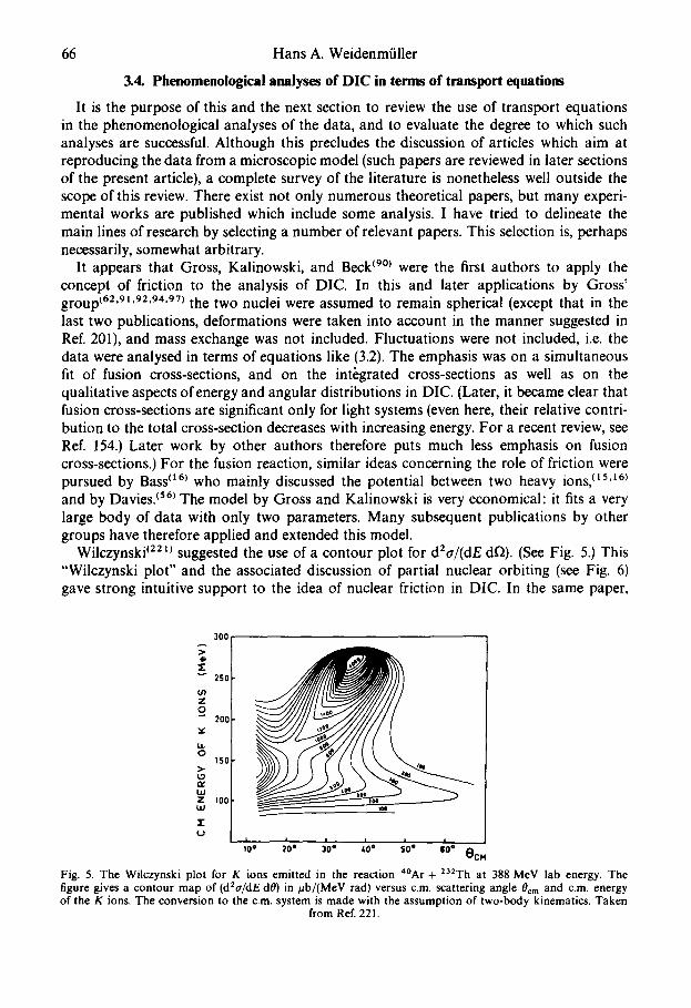
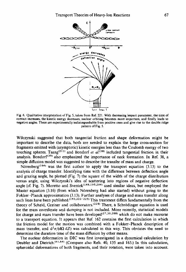
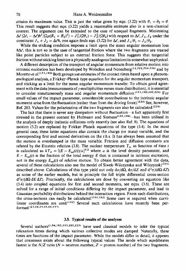
Wilczynski (221J suggested the use of a contour plot for d2tr/(dE dr2). (See Fig. 5.) This "Wilczynski plot" and the associated discussion of partial nuclear orbiting (see Fig. 6) gave strong intuitive support to the idea of nuclear friction in DIC. In the same paper,
25O 0 200[
150 g
o z '°°[ - - - - ;o. 1o. ;o. ;o. ;o- ec.
Fig. 5. The Wilczynski plot for K ions emitted in the reaction 4°Ar + 232Th at 388 MeV lab energy. The figure gives a contour map of (d2a/dE dO) in/zb/(McV rad) versus c.m scattering angle 0cm and c.m. energy of the K ions. The conversion to the cm. system is made with the assumption of two-body kinematics. Taken
from Ref. 222.
E I . ~ c r o , , ,,ct,o~
-Ograz O* cegra, I energy decre-
Transport Theories of Heavy-Ion Reactions 67
[cr,t Lmax t
Fig. 6. Qualitative interpretation of Fig. 5, taken from Ref. 221. With decreasing impact parameter, the time of contact increases, the kinetic energy decreases, nuclear orbiting becomes more important, and finally leads to negative angles. These are experimentally indistinguishable from positive ones and give rise to the double ridge
pattern of Fig. 5.
Wilczynski suggested that both tangential friction and shape deformation might be important to describe the data, both are needed to explain the large cross-section for fragments emitted with (asymptotic) kinetic energies less than the Coulomb energy of two touching spheres. Tsang (2~1) and Bondorf et al. (3a) included tangential friction in their analysis. Bondorf (ag) also emphasized the importance of neck formation. In Ref. 38, a simple diffusion model was suggested to describe the transfer of mass and charge.
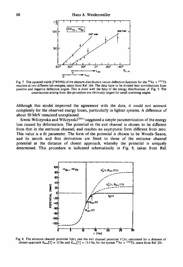
N6renberg "64) was the first author to apply the transport equation (3.13) to the analysis of charge transfer. Identifying time with the difference between deflection angle and grazing angle, he plotted (Fig. 7) the square of the width of the charge distribution versus angle, using Wilczynski's idea of scattering into regions of negative deflection angle (cf. Fig. 7). Moretto and Sventek "48'15°'2°4~ used similar ideas, but employed the Master equation (3.16) (from which N6renberg had also started) without going to the Fokker-Planck approximation (3.13). Further analyses of charge and mass transfer along such lines have been published. °9 a.222-225~ This treatment differs fundamentally from the theory of Scheid, Greiner and collaborators. (22a~ There, a Schr6dinger equation is used for the mass coordinate and damping is not included. More recently, statistical models for charge and mass transfer have been developed t2~'3°'2°°~ which do not make recourse to a transport equation. It appears that Ref. 162 contains the first calculation in which the friction model for the motion was combined with a Fokker-Planck description of mass transfer, and d2a/(dfl dZ) was calculated in this way. This obviates the need to determine the duration time of the mass diffusion by other means.
The nuclear deformation in DIC was first investigated in a dynamical calculation by Deubler and Dietrich. t6~'6.) (Compare also Refs. 40, 135 and 163.) In this calculation, spheroidal deformations of both fragments, and their rotation, were taken into account.
68
100 i
50
60*
Hans A. Weidenmiiller
1 I i I ! 1 I f f |
123 ,.. 3 8 8 ~ _ 297 MIV , ~ "
f * f ~ / l [ J J l l l t 40" 20" 0.* -20* -40"
~O a, ~int O c m 0 ~ "tint
Fig. 7. The squared width ( F W H M ) o f the element distribution versus deflection function for the 4°Ar + 23ZTh reaction at two different lab energies, taken from Ref. 164. The data have to be divided into contributions from positive and negative deflection angles. This is done with the help of the energy distributions, cf. Fig. 5. The
uncertainties arising from this procedure are obviously largest for small scattering angles.
Although this model improved the agreement with the data, it could not account completely for the observed energy losses, particularly in lighter systems. A difference of about 50 MeV remained unexplained.
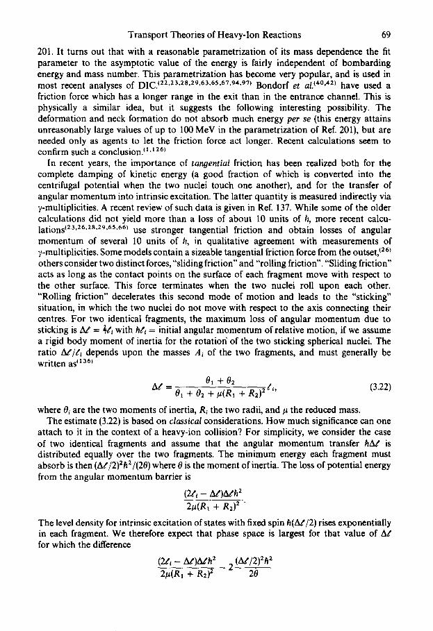
Siwek-Wilczynska and Wilczynski ~2°t~ suggested a simple parametrization of the energy loss caused by deformation. The potential in the exit channel is chosen to be different from that in the entrance channel, and reaches an asymptotic form different from zero. This value is a fit parameter. The form of the potential is chosen to be Woods-Saxon, and its zeroth and first derivatives are fitted to those of the entrance channel potential at the distance of closest approach, whereby the potential is uniquely determined. This procedure is indicated schematically in Fig. 8, taken from Ref.
100
SO
GO
/,0
0
Z ~ -&0
-80
°
0
4OAr. 231Th V~ (r.Rm, n [2])
s s S ~
/ 11 V~( r, Rm, n 1111
/ f " V~(rl
/ Rmin 121 I !
/ /
/
I S
I It I I
10 ~ 20 2S 30 r ( f ro)
Fig. 8. The entrance channel potential Vd(r), and the exit channel potential V~(r). calculated for a distance of closest approach Rm~,[2] = 12 fm and R,,~,[l] = 13.5 fro, for the system '*°Ar + '32Th, taken from Ref. 201.
Transport Theories of Heavy-Ion Reactions 69
201. It turns out that with a reasonable parametrization of its mass dependence the fit parameter to the asymptotic value of the energy is fairly independent of bombarding energy and mass number. This parametrization has become very popular, and is used in most recent analyses of D I C . (22'23'28'29'63'65'67'94'97~ Bondorf et al. ~4°'~2~ have used a friction force which has a longer range in the exit than in the entrance channel. This is physically a similar idea, but it suggests the following interesting possibility. The deformation and neck formation do not absorb much energy per se (this energy attains unreasonably large values of up to 100 MeV in the parametrization of Ref. 201), but are needed only as agents to let the friction force act longer. Recent calculations seem to confirm such a conclusion3 t,~ 26)
In recent years, the importance of tanyential friction has been realized both for the complete damping of kinetic energy (a good fraction of which is converted into the centrifugal potential when the two nuclei touch one another), and for the transfer of angular momentum into intrinsic excitation. The latter quantity is measured indirectly via ~/-multiplicities. A recent review of such data is given in Ref. 137. While some of the older calculations did not yield more than a loss of about 10 units of/I, more recent calcu- lations (23'26'2s'29'65"66~ u s e stronger tangential friction and obtain losses of angular momentum of several 10 units of h, in qualitative agreement with measurements of 7-multiplicities. Some models contain a sizeable tangential friction force from the outseL ~26~ others consider two distinct forces, "sliding friction" and "rolling friction". "Sliding friction" acts as long as the contact points on the surface of each fragment move with respect to the other surface. This force terminates when the two nuclei roll upon each other. "Rolling friction" decelerates this second mode of motion and leads to the "sticking" situation, in which the two nuclei do not move with respect to the axis connecting their centres. For two identical fragments, the maximum loss of angular momentum due to sticking is At' = ~t't with ht'i = initial angular momentum of relative motion, if we assume a rigid body moment of inertia for the rotatior/of the two sticking spherical nuclei. The ratio Az'/t', depends upon the masses A~ of the two fragments, and must generally be written as ~t 36~
0t +02 At'
0t + 02 +/~(R1 + R2) 2t'i' (3.22)
where 0~ are the two moments of inertia, R~ the two radii, and # the reduced mass. The estimate (3.22) is based on classical considerations. How much significance can one
attach to it in the context of a heavy-ion collision? For simplicity, we consider the case of two identical fragments and assume that the angular momentum transfer hAt' is distributed equally over the two fragments. The minimum energy each fragment must absorb is then (Ag/2)2h2/(20) where 0 is the moment of inertia. The loss of potential energy from the angular momentum barrier is
(2g~- AZ)At'h 2
2#(Rl + R2) 2 '
The level density for intrinsic excitation of states with fixed spin h(At'/2) rises exponentially in each fragment. We therefore expect that phase space is largest for that value of At' for which the difference
(2all -- At')/~'fi 2 2 (Ad/2)2h2 2#(Rt + R2) 2 20
70 Hans A. Weidenmiiller
attains its maximum value. This is just the value given by eqn. (3.22) with 0t = 02 = 0. This result suggests that eqn. (3.22) yields a reasonable estimate also in a non-classical context. The argument can be extended to the case of unequal fragments. Minimising At" (2:i - Al)h2/(21a(Rl + R2) 2) - J2/(201) - J2 / (202)wi th respect to At', J~, J2 under the constraint J~ + J2 = A/h, one again finds eqn. (3.22) for At', and J1/01 = J2/02.
While the sticking condition imposes a limit upon the mean angular momentum loss hA/', this is not so in the case of tangential friction where the two fragments are treated like point particles subject to an external friction force. This suggests that tangential friction without sticking limit (or a physically analogous limitation) is somewhat unphysical.
A different description of the transport of angular momentum from relative motion into intrinsic excitation has been developed by Wolschin and Norenberg (12'222'224'2261 and by Moretto et al. t~ s3,1 so) Both groups use estimates of the contact times based upon a phenom- enological analysis, a Fokker-Planck type equation for the angular momentum transport, and sticking as a limit for the mean angular momentum transfer. To obtain good agree- ment with the data (measurements of),-multiplicities versus mass distribution), it is essential to consider simultaneously mass and angular momentum diffusion: 153'1s°'2°5'224) For small values of the impact parameter, considerable contributions to the intrinsic angular momenta arise from the fluctuation (rather than from the driving force): 224) See, however, Ref. 203. Values for the polarization of the two fragments can also be calculated. (226)
The fact that there is never any dissipation without fluctuation--a fact apparently first stressed in the present context by Hofmann and Siemens (l °5'l°6)-- has been utilised in the analysis of deeply inelastic collisions only recently (see also Ref. 8). The equations of motion (3.2) are replaced by Fokker-Planck equations of the type (3.4). In the most general case, these latter equations also contain the charge (or mass) variable, and the corresponding first and second derivatives on the r.h.s. It has always been assumed that the motion is overdamped in the mass variable. Friction and diffusion constants are related by the Einstein relation (3.8). The nuclear temperature Too as function of time t is calculated as kToo = I ( E - Ercl(t))/al 1/2 where a is the level density parameter, and E - Ere~(t) is the fraction of the total energy E that is contained in intrinsic excitation, not in the energy Er~t(t) of relative motion. To obtain better agreement with the data, several of these calculations also use the model of Siwek-Wilczynska and Wilczynski (2° ~) described above. Calculations of this type yield not only dtr/df~, d a / d Z and d2tr/(df~ dZ) as some of the earlier models, but in principle the full triple differential cross-section d3tr/(df~dEdZ). Practically, the calculations are done by converting an equation like (3.4) into coupled equations for first and second moments, see eqns. (3.6). These are solved for a range of initial conditions differing by the impact parameter, and lead to Gaussian probability distributions behind the interaction region. From such distributions, the cross-sections can easily be calculated. (t61'1621 Some care is required when curvi- linear coordinates are used. (~62) Several such calculations have recently been per- formed.(23,28,29.65.66.197)
3.5. Typical results of the analyses
Several authors O'94.la2,t93,2°5.225) have used classical models to infer the typical relaxation times during which various collective modes are damped. Naturally, these times are functions of the impact parameter. While the models differ in detail, it appears that consensus exists about the following typical values. The mode which equilibrates fastest is the N / Z ratio (N = neutron number, Z = proton number) of the two fragments.
Transport Theories of Heavy-Ion Reactions 71
The experimental evidence for this statement is discussed in Section 111.9 of Ref. 136 where it is suggested that a typical relaxation time for this mode is xn/z < 10 -22 s. This fact is little understood. ~5°~ The short time suggests that this process is not a statistical relaxation phenomenon3 t3s~ The radial part of the kinetic energy is dissipated faster than the angular part, typical numbers being ~s2'225'226~ xrad~ 3. .5 x 10-22s and Z a . g ~ 10-21 s. Deformations of the fragments develop during typical times ~'ts2'22s~ ¢def "" 1 .. 5 X 10- 2 ~ S. The contact time is typically "t'cont ~, 1... 5 X 10- 21 S depending upon the impact parameter. These values agree with those of recent calculations using time- dependent Hartree-Fock theory. ~59~ Table 1 summarizes these numbers. It should be borne in mind that the numbers are only semiquantitative, and that different analyses might produce numbers differing by factors of two or so.
Table 1. Typical relaxation times for various collective modes
~'~ 'z "Crad '~ang ~def Zcontact
<10-22s 3 . . 5 x 10-22s 1 0 - ' t s l . . 5 x 10⁻²ts 1 . . 5 x l 0 - 2 J s
The mass diffusion has sometimes been analysed under the assumption that the mass exchange corresponds to an overdamped motion. This is valid if YAI >> COcoU where COco" is the collective frequency of the mass variable AI, the mass of fragment 1. Using the numbers given in Ref. 228 and a value DA = 15" 1022 s- 1 for the 23sU + 23SU reaction (see Table 2 on p. 81), one finds COco, ~ 102ts - t and, from eqn. (3.11), "/A, = 1022S - t , SO that indeed "/A, >> COcon. The value of ~:A~ suggests that the collective coordinate canonically conjugate to the mass At on one fragment equilibrates in times ~ 10 -22 s, see eqn. (3.7). This condition must be met for the model of overdamped motion to be applicable, cf. Section 3.2. We note that 10 -22 s is a remarkably short time, comparable to ~s/z. It is not clear whether for such short time intervals a transport description is meaningful, cf. Section 4.1. Other analyses do not consider the mass a collective variable, and describe mass exchange simply as a random-walk problem. To these approaches, the remarks just made obviously do not apply. A common feature of both approaches is that the mass drift does not terminate during the contact time. See, however, Ref. 182.
In dynamical calculations employing equations of motion with friction forces, or diffusion equations of Fokker-Planck type, the inertia parameter is, with few exceptions, taken to be the reduced mass of relative motion, and the rigid body moment of inertia for relative and intrinsic rotation. In the context of heavy-ion scattering, the proper choice of the inertia parameter seems to have received little attention3t°6't°7'lt° ' t s2~ In contra- distinction, a considerable body of work exists on the conservative potential between two heavy ions335,45,46,58,71, 130,131,151,163,208) Two different approaches have been taken: The potential has been calculated in the "sudden" or "frozen density" approximation, in which the density distribution of each fragment is not given the time to readjust to the presence of the other fragment, or in the "adiabatic" approximation, in which the converse is true. From the numbers listed in Table 1 and the qualitative aspects of the analyses reported below, it appears that the frozen density approximation is the better alternative during the initial stages of the reaction, and the adiabatic approximation is better towards the end. No calculation exists that takes into account this time change of the average potential.
72 Hans A. Weidenmiiller
For small overlap between the two ions, a folded potential {'*s'7~) can be used. This potential is determined by
V~°'=fd3rtld3r2p1(r,)p2(r2)Vl2(r-r,-r2), (3.23)
where I/i 2 is the effective two-body interaction, r the distance between the two centres, and p~ the frozen densities of both fragments. This potential does not account for the repulsion which at small distances is caused by the exclusion principle, or for saturation effects. Exchange and saturation effects are important already at distances of closest approach reached in DIC. Therefore, the folded potential is not very well suited for a description of the DIC. A considerable improvement can be attained by using a saturating Skyrme force, and by approximately taking into account exchange effects. ~46'2°s~ These calculations do not use the simple formula (3.23), but instead the Skyrme energy density functional in a manner first suggested by Brueckner et al. ~43'44~ Calculations also using Brueckner's formalism but a more phenomenological ansatz for the energy density have also been carried out. ~14's'1 These calculations have been improved by using some results of Hartree-Fock calculations. ~21.1 s o~
A macroscopic approach to the same problem consists in using the liquid drop model, and in calculating potential energy surfaces for a chosen set of shape parameters. In this way, a calculation with some semblance to an adiabatic calculation is performed. For two drops coming in contact, it is necessary to take into account the finite range of the nuclear force to get a valid expression, t13°'131~ Potential energy surfaces have been calculated this way. ~ s. 132. t 5 t., 63~
Another method, most often applied in the frame of the frozen density approximation, determines the "proximity potentiar', c35~ It is assumed that the surface thickness of nuclei is small compared to their radius of curvature. Then it is possible to express the potential between two heavy ions in terms of the interaction potential per unit area between two flat surfaces, and the curvature.
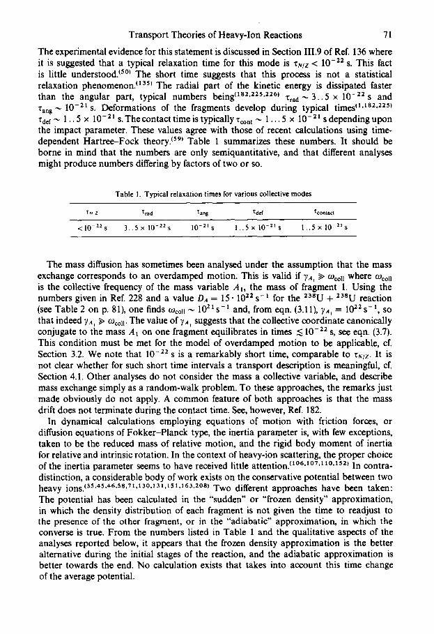
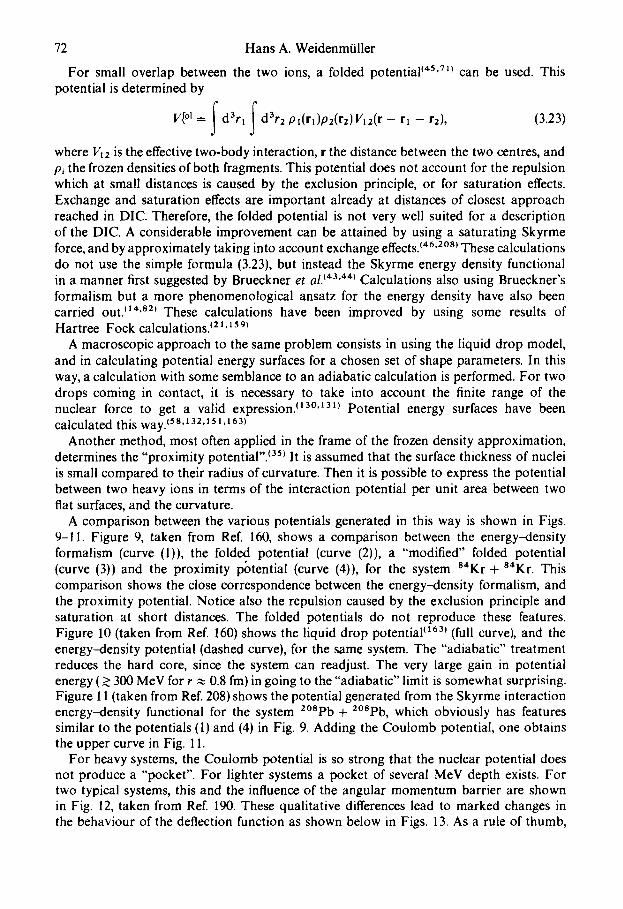
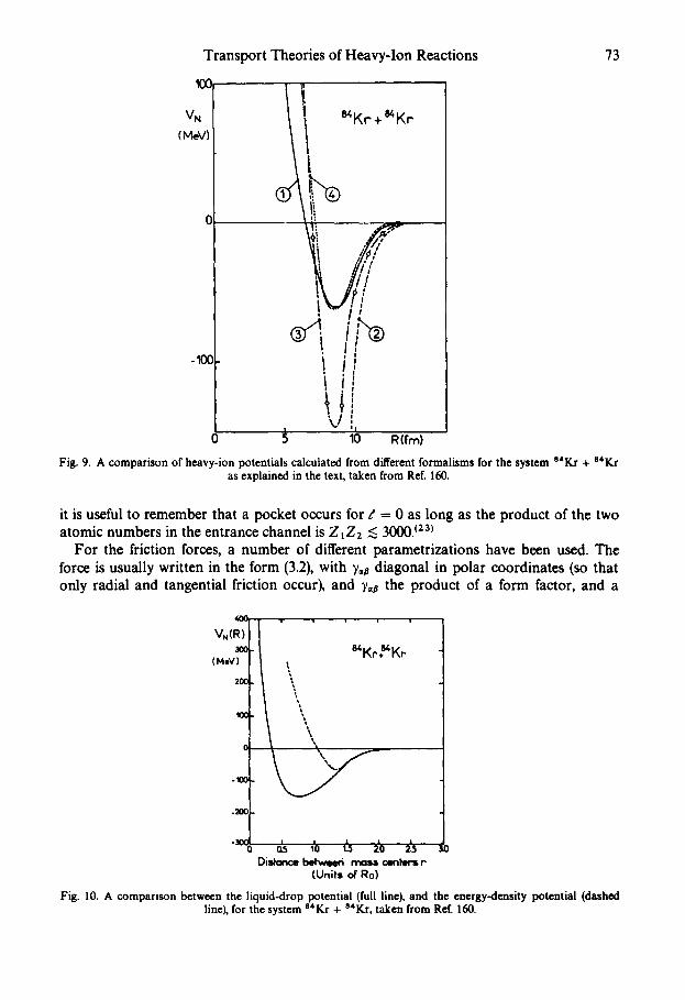
A comparison between the various potentials generated in this way is shown in Figs. 9-11. Figure 9, taken from Ref. 160, shows a comparison between the energy--density formalism (curve (1)), the folded potential (curve (2)), a "modified" folded potential (curve (3)) and the proximity potential (curve (4)), for the system 84Kr + 84Kr. This comparison shows the close correspondence between the energy--density formalism, and the proximity potential. Notice also the repulsion caused by the exclusion principle and saturation at short distances. The folded potentials do not reproduce these features. Figure 10 (taken from Ref. 160) shows the liquid drop potential t~63~ (full curve), and the energy-density potential (dashed curve), for the same system. The "adiabatic" treatment reduces the hard core, since the system can readjust. The very large gain in potential energy ( ~> 300 MeV for r ,~ 0.8 fm) in going to the "adiabatic" limit is somewhat surprising. Figure 11 (taken from Ref. 208) shows the potential generated from the Skyrme interaction energy-density functional for the system 2°Spb + 2°Spb, which obviously has features similar to the potentials (1) and (4) in Fig. 9. Adding the Coulomb potential, one obtains the upper curve in Fig. 1 I.
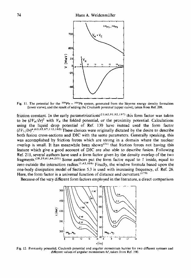
For heavy systems, the Coulomb potential is so strong that the nuclear potential does not produce a "pocket". For lighter systems a pocket of several MeV depth exists. For two typical systems, this and the influence of the angular momentum barrier are shown in Fig. 12, taken from Ref. 190. These qualitative differences lead to marked changes in the behaviour of the deflection function as shown below in Figs. 13. As a rule of thumb,
Transport Theories of Heavy-Ion Reactions 73
VN ! ~Kr+~Kr
L
-100 i
, , I |
0 ~ 10 R If m)
Fig. 9. A comparison of heavy-ion potentials calculated from different formalisms for the system S=Kr + S4Kr as explained in the text, taken from Ref. 160.
it is useful to remember that a pocket occurs for d = 0 as long as the product of the two atomic numbers in the entrance channel is Z,Z2 ~< 3000. (23)
For the friction forces, a number of different parametrizations have been used. The force is usually written in the form (3.2), with Y=B diagonal in polar coordinates (so that only radial and tangential friction occur), and y=a the product of a form factor, and a
cMv l \ o K:K
\
Dishmce betv,~¢i moss csot~rs r {Units of R0)
Fig. 10. A comparison between the liquid-drop potential (full line), and the energy-density potential (dashed line), for the system S4Kr + S'Kr, taken from Ref. 160.
74 Hans A. Weidenmfi l ler
700
600
• 20
0 •
-20
-60
?O~p b .?o~pb
N + VC
w,.
V N ,, ,, ,, ,, ,? '? ....
i i | | i i
Fig. 11. The potential for the 2°aPb + 2°Spb system, generated from the Skyrme energy density formalism (lower curve), and the result of adding the Coulomb potential (upper curve), taken from Ref. 208.
friction constant. In the early parametrizations (23'62"91.92,197) this form factor was taken to be (3VN/Or) 2 with VN the folded potential, or the proximity potential. Calculations using the liquid drop potential of Ref. 130 have instead used the form factor (C 3 Vv/~r),l..(63.65,67,112,162) These choices were originally dictated by the desire to describe both fusion cross-sections and DIC with the same parameters. Generally speaking, this was accomplished by friction forces which are strong in a domain where the nuclear overlap is small. It has meanwhile been shown (at) that friction forces not having this feature which give a good account of DIC are also able to describe fusion. Following Ref. 211, several authors have used a form factor given by the density overlap of the two fragments. (2a'29'61'6'*'2°1) Some authors put the form factor equal to I inside, equal to zero outside the interaction radius. (z'42'~°6) Finally, the window formula based upon the one-body dissipation model of Section 5.3 is used with increasing frequency, cf. Ref. 26. Here, the form factor is a universal function of distance and curvature. (t79)
Because of the very different form factors employed in the literature, a direct comparison
140 . . . . . . .
500 I~ I I ~ 120 ! 12
{ 350 80 sm
30O
8 10 t2 14 16 6 8 10 ~2 ]4
Fig. 12. Proximity potential, Coulomb potential and angular momentum barrier for two different systems and different values of angular momentum ht', taken from Re£ 190.
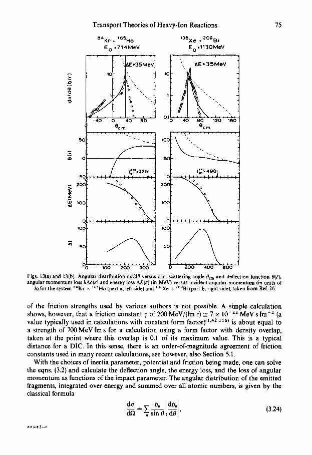
Transport Theories of Heavy-Ion Reactions 75
A L
.D
(Z) 'O
o 'O
>, :£ uJ , 13
,,:3
5C
-5o 2 ~
~ o o
o 10o
50
e4Kr, ,, 165H0
E 0 . 7 1 4 M e V
IC
I
-40 0
, . , . ,
E ..35MeV"
o \ \
/ ". o
o
z o ,
40 80 OC m
. . . . I . . . . . i . . . . t • •
. . . . I . , - : : I : : : : t a . o °
o
o o -
I00 2o0 30o
10
1
o.1
13eXe . 2°9p, i
E 0 . ,1130MeV
Z 40
& E ~ 3 5 M e V
80 120 160 e¢.m.
':!i iilJ Figs. 13(a) and 13(b). Angular distribution da/dO versus c.m. scattering angle 0m and deflection function 0(~'), angular momentum loss hAt'(l) and energy loss AE(/) (in MeV) versus incident angular momentum (in units of
h) for the system a'Kr + ~"~Ho (part a, left side) and ta6Xe + Z°gBi (part b, right side), taken from Ref. 26.
of the friction strengths used by various authors is not possible. A simple calculation shows, however, that a friction constant 7 of 200 MeV/(fm c) ~ 7 x 10 -22 MeV s fm -2 (a value typically used in calculations with constant form factor) (1'42J ~6) is about equal to a strength of 700 MeV fm s for a calculation using a form factor with density overlap, taken at the point where this overlap is 0.1 of its maximum value. This is a typical distance for a DIC. In this sense, there is an order-of-magnitude agreement of friction constants used in many recent calculations, see however, also Section 5.1.
With the choices of inertia parameter, potential and friction being made, one can solve the eqns. (3.2) and calculate the deflection angle, the energy loss, and the loss of angular momentum as functions of the impact parameter. The angular distribution of the emitted fragments, integrated over energy and summed over all atomic numbers, is given by the classical formula
do '=x7 b, db, , (3.24)
~ sin 0 d0
P.P .N .P3 - -F
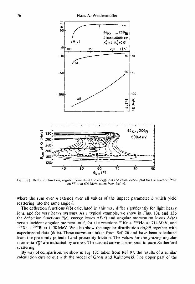
76 o
5O
10
-10
-50
- 1 0 0
Hans A. Weidenmfiller
f /~e 8Z'Kr " 209Bi
E I I o b I = 6 0 0 M e V eLI ° =,., Kg,0 0,
100 1.50 200 Ll'h ] t ~ I
10-
50_
~E ~ ~
-10
-50
- 1 0 0
o
W <~
i
84Kr. 209Bi 320 ,.00. i-.--0,.~,~/~ 600MeV
120 ,o I I I 1 I
t,O 50 60 70 80 Oc m [o]
90
Fig. 13(c). Deflection function, angular momentum and energy loss and cross-section plot for the reaction S4Kr on 2°'~Bi at 600 MeV, taken from Ref. 97.
where the sum over n extends over all values of the impact parameter b which yield scattering into the same angle 0.
The deflection functions O(b) calculated in this way differ significantly for light heavy ions, and for very heavy systems. As a typical example, we show in Figs. 13a and 13b the deflection functions 0(E), energy losses AE({) and angular momentum losses AK'(E) versus incident angular momentum g, for the reactions 84Kr + 165Ho at 714 MeV, and z36Xe + 2°9Bi at 1130 MeV. We also show the angular distribution da/d0 together with experimental data (dots). These curves are taken from Ref. 26 and have been calculated from the proximity potential and proximity friction. The values for the grazing angular momenta f~P are indicated by arrows. The dashed curves correspond to pure Rutherford scattering.
By way of comparison, we show in Fig. 13c, taken from Ref. 97, the results of a similar calculation carried out with the model of Gross and Kalinowski. The upper part of the
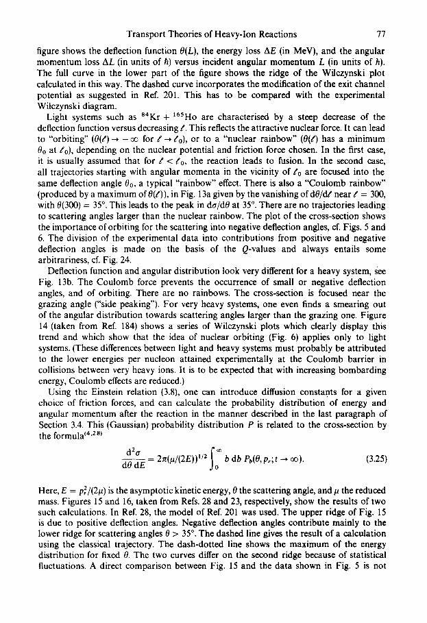
Transport Theories of Heavy-Ion Reactions 77
figure shows the deflection function O(L), the energy loss AE (in MeV), and the angular momentum loss AL (in units of h) versus incident angular momentum L (in units of h). The full curve in the lower part of the figure shows the ridge of the Wilczynski plot calculated in this way. The dashed curve incorporates the modification of the exit channel potential as suggested in Ref. 201. This has to be compared with the experimental Wilczynski diagram.
Light systems such as S4Kr + 165Ho are characterised by a steep decrease of the deflection function versus decreasing :. This reflects the attractive nuclear force. It can lead to "orbiting" (0 ( : )~ - o v for : -- , t'o), or to a "nuclear rainbow" (0(:) has a minimum 0o at :o), depending on the nuclear potential and friction force chosen. In the first case, it is usually assumed that for : < :o, the reaction leads to fusion. In the second case, all trajectories starting with angular momenta in the vicinity of t'0 are focused into the same deflection angle 0o, a typical "rainbow" effect. There is also a "Coulomb rainbow" (produced by a maximum of 0(:)), in Fig. 13a given by the vanishing of d0/clf near t' = 300, with 0(300) = 35 °. This leads to the peak in do~dO at 35 °. There are no trajectories leading to scattering angles larger than the nuclear rainbow. The plot of the cross-section shows the importance of orbiting for the scattering into negative deflection angles, cf. Figs. 5 and 6. The division of the experimental data into contributions from positive and negative deflection angles is made on the basis of the Q-values and always entails some arbitrariness, cf. Fig. 24.
Deflection function and angular distribution look very different for a heavy system, See Fig. 13b. The Coulomb force prevents the occurrence of small or negative deflection angles, and of orbiting. There are no rainbows. The cross-section is focused near the grazing angle ("side peaking"). For very heavy systems, one even finds a smearing out of the angular distribution towards scattering angles larger than the grazing one. Figure 14 (taken from Ref. 184) shows a series of Wilczynski plots which clearly display this trend and which show that the idea of nuclear orbiting (Fig. 6) applies only to light systems. (These differences between light and heavy systems must probably be attributed to the lower energies per nucleon attained experimentally at the Coulomb barrier in collisions between very heavy ions. It is to be expected that with increasing bombarding energy, Coulomb effects are reduced.)
Using the Einstein relation (3.8), one can introduce diffusion constants for a given choice of friction forces, and can calculate the probability distribution of energy and angular momentum after the reaction in the manner described in the last paragraph of Section 3.4. This (Gaussian) probability distribution P is related to the cross-section by the formula ~4'2s)
d2° f ~ d ~ E = 2;t(#/(2E))t/2 b db Pb(O,p,;t --* or). (3.25) 0
Here, E = p2/(2/~) is the asymptotic kinetic energy, 0 the scattering angle, and # the reduced mass. Figures 15 and 16, taken from Refs. 28 and 23, respectively, show the results of two such calculations. In Ref. 28, the model of Ref. 201 was used. The upper ridge of Fig. 15 is due to positive deflection angles. Negative deflection angles contribute mainly to the lower ridge for scattering angles 0 > 35 °. The dashed line gives the result of a calculation using the classical trajectory. The dash-dotted line shows the maximum of the energy distribution for fixed 0. The two curves differ on the second ridge because of statistical fluctuations. A direct comparison between Fig. 15 and the data shown in Fig. 5 is not
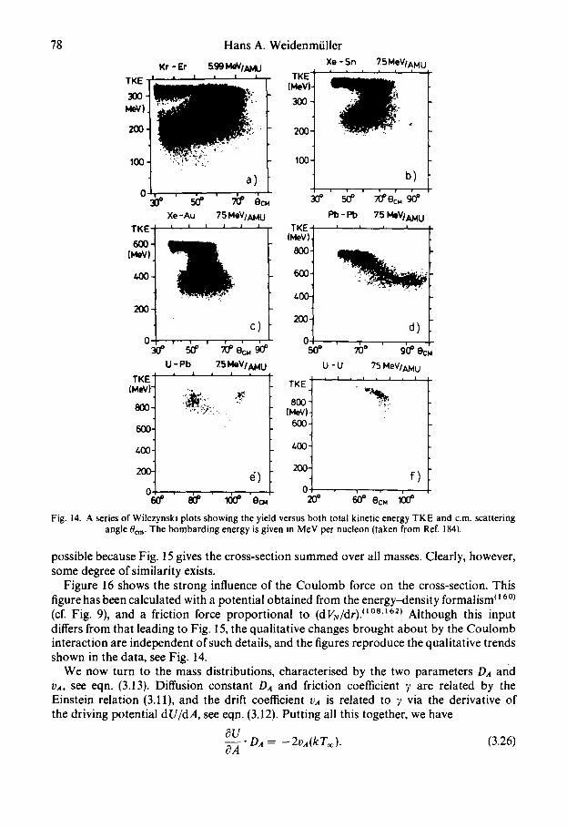
78
TKE "
300- MeV).
I ,. ~ ' ~ ' - "
0 j
TKE
600- (MeV)
tOO
2OO
0
TKE {MeV)"
600-
4IX)-
Kr - E~ r
|
|
Xe -Au I I
U - P b
.~ . : : . : .
Hans A. Weidenmfiller
599 MeVIAMU Xe - Sn l , , L T K E j " '
: " 200-4
~ ) 75 MeVIAMU
i J | l
c)-
~ e ~ 75 MeV I AMU
| ,
~)
100,
30*
TKE (MeV)
800-
600-
400-
200-
0 50*
TKE i
1 400-1
200-4
75MeV/AM U I ~ I A ,
b)
' ~ ' -~e~.o~ Pb - lab 75 MeVIAMU
d) ' 76* ' 9 b * e e .
U - U 75 MeVIAMu • 1 , I i 1 , 1
f) 0 (
0 ab* ' ~o* "e= 20* ~* e~..he Fig. 14. A series of Wilczynski plots showing the yield versus both total kinetic energy TKE and c.m. scattering
angle 0cm. The bombarding energy is given in MeV per nucleon (taken from Ref. 184).
possible because Fig. 15 gives the cross-section summed over all masses. Clearly, however, some degree of similarity exists.
Figure 16 shows the strong influence of the Coulomb force on the cross-section. This figure has been calculated with a potential obtained from the energy-density formalism (~ 60) (cf. Fig. 9), and a friction force proportional to (dl(N/dr). (l°a't62) Although this input differs from that leading to Fig. 15, the qualitative changes brought about by the Coulomb interaction are independent of such details, and the figures reproduce the qualitative trends shown in the data, see Fig. 14.
We now turn to the mass distributions, characterised by the two parameters Da and vA, see eqn. (3.13). Diffusion constant D,4 and friction coefficient Y are related by the Einstein relation (3.11), and the drift coefficient v,4 is related to 7 via the derivative of the driving potential dU/dA, see eqn. (3.12). Putting all this together, we have
8U - - " Da = - 2vA (k To~). (3.26) dA
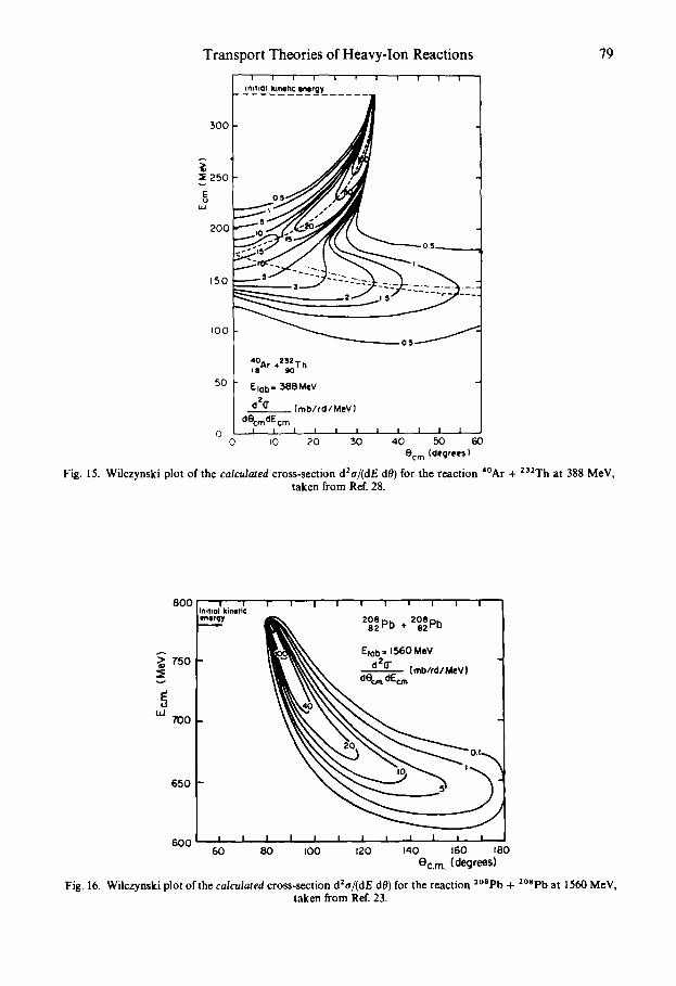
Transport Theories of Heavy-Ion Reactions I i I I i f I i I I i
l f l l l lO l k l f~ I t lC im41rgy
300 -
=
o s ~ / " / / / , k , ~ v J
50
1 I 0 I 1 1 0 0 4 ,50 6 0
Ocm ( d e g r e e s )
40 232 T - I 8 A r + 90
F l o b " 3 8 8 M e V
dzO" ( m b / r d / M e V ]
d e c m d l r cm l 1 | I 1 I
iO 20 30
79
Fig. 15. Wilczynski plot of the calculated cross-section d2a/(dE dO) for the reaction 4°Ar + 232Th at 388 MeV, taken from Ref. 28.
800
~'~ T50
70O
650
! I In i t io l kinetic In i l r~¥
m
I | I ! 1 I I I I
2 0 8 2 0 8 8zPb 4. szPb
6 0 0 I I I 1 1 I I I I I I I
6o 80 eoo t2o 14o s6o t8o ec.m. (degrees)
Fig. 16. Wilczynski plot of the calculated cross-section d2a/(dE dO) for the reaction a°Spb + 2°Spb at 1560 MeV, taken from Ref. 23.
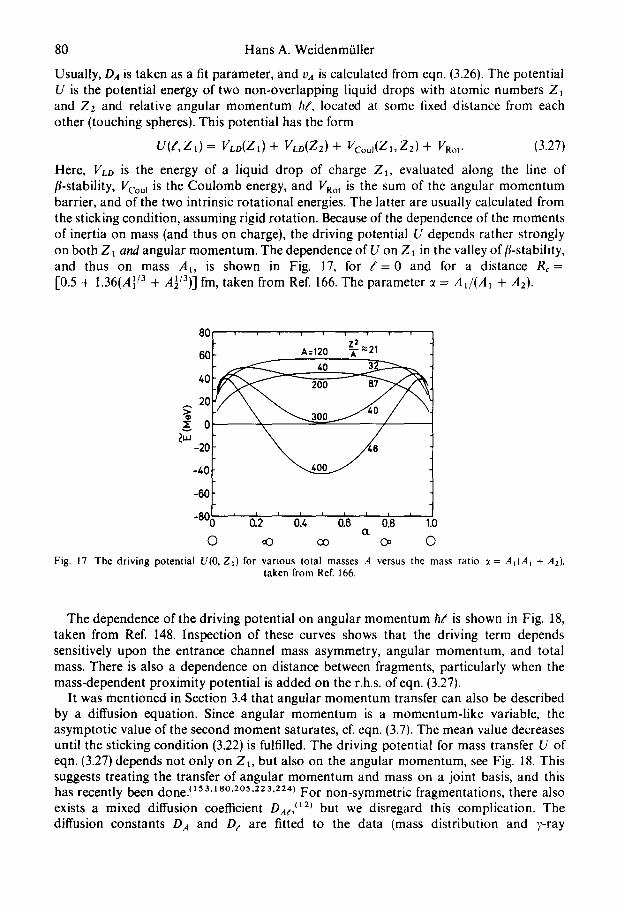
80 Hans A. Weidenmiiller
Usually, D,4 is taken as a fit parameter, and va is calculated from eqn. (3.26). The potential U is the potential energy of two non-overlapping liquid drops with atomic numbers Zl and Z2 and relative angular momentum hd. located at some fixed distance from each other (touching spheres). This potential has the form
U ( d , Z , ) = VLD(ZI)+ VLD(Z2)+ Vcoul (Zt ,Z2)+ FRo t. (3.27)
Here, VLD is the energy of a liquid drop of charge Zt, evaluated along the line of //-stability, Vcoul is the Coulomb energy, and VRo t is the sum of the angular momentum barrier, and of the two intrinsic rotational energies. The latter are usually calculated from the sticking condition, assuming rigid rotation. Because of the dependence of the moments of inertia on mass (and thus on charge), the driving potential U depends rather strongly on both Zl and angular momentum. The dependence of U on Zt in the valley of/i-stability, and thus on mass At, is shown in Fig. 17, for : = 0 and for a distance R , = [0.5 + 1.36(A~/3 + AI/3)] fm, taken from Ref. 166. The parameter ~t = At/(At + A2).
80 / . . . . . . . . . Z 2
60 I . A=120 ~--~21
V \ 10 ~8 -20
-/*0
- 6 0
-80 ' 0.2 ©
I I I I I I I
0.4 0.6 0.8 1.0
co o, ©
Fig. 17. The driving potential U(0, Z~) for various total masses A versus the mass ratio ~ = At(At + A2), taken from Ref. 166.
The dependence of the driving potential on angular momentum h{ is shown in Fig. 18, taken from Ref. 148. Inspection of these curves shows that the driving term depends sensitively upon the entrance channel mass asymmetry, angular momentum, and total mass. There is also a dependence on distance between fragments, particularly when the mass-dependent proximity potential is added on the r.h.s, of eqn. (3.27).
It was mentioned in Section 3.4 that angular momentum transfer can also be described by a diffusion equation. Since angular momentum is a momentum-like variable, the asymptotic value of the second moment saturates, cf. eqn. (3.7). The mean value decreases until the sticking condition (3.22) is fulfilled. The driving potential for mass transfer U of eqn. (3.27) depends not only on ZI, but also on the angular momentum, see Fig. 18. This suggests treating the transfer of angular momentum and mass on a joint basis, and this has recently been done: t53.180.205,223,224) For non-symmetric fragmentations, there also exists a mixed diffusion coefficient DA:, t12) but we disregard this complication. The diffusion constants DA and D: are fitted to the data (mass distribution and ;,-ray
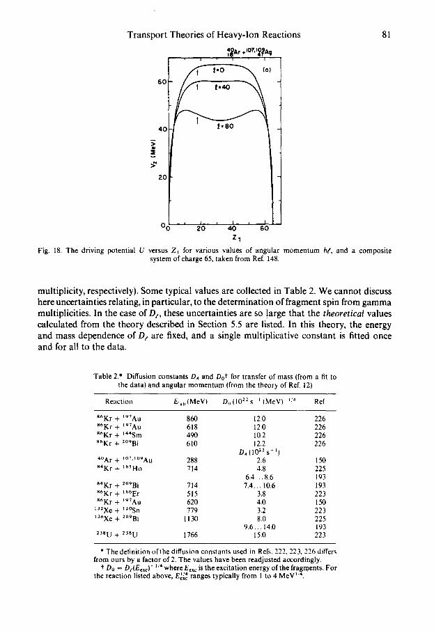
l , I
6O
40
0 o
Transport Theories of Heavy-Ion Reactions
, 1 , 1 , 1 2 0 4 0 60
Zl
81
Fig. 18. The driving potential U versus Zt for various values of angular momentum h/, and a composite system of charge 65, taken from Ref. 148.
multiplicity, respectively). Some typical values are collected in Table 2. We cannot discuss here uncertainties relating, in particular, to the determination of fragment spin from gamma multiplicities. In the case of Dr, these uncertainties are so !arge that the theoretical values calculated from the theory described in Section 5.5 are listed. In this theory, the energy and mass dependence of D: are fixed, and a single multiplicative constant is fitted once and for all to the data.
Table 2.* Diffusion constants DA and Do~" for transfer of mass (from a fit to the data) and angular momentum Ifrom the theory of Ref. 12)
Reaction Elah(MeV} Du{1022s ' (MeV) 'a Ref
S6Kr + l ~ A u 860 12.0 226 S6Kr + 19TAB 618 12.0 226 86Kr + 1"4Sm 490 10.2 226 S6Kr + 2°°Bi 610 12.2 226
D~ (10 2z s- t) 4°Ar + l°7'l°gAu 288 2.6 150 84Kr -,- t6SHo 714 4.8 225
6.4... 8.6 193 84Kr + 2°9Bi 714 7.4... 10.6 193 "°Kr + 166Er 515 3.8 223 86Kr + l°TAu 620 4.0 150
132Xe + 12°Sn 779 3.2 223 136Xe + 2°9Bi 1130 8.0 225
9.6.. . 14.0 193 238U + 238U 1766 15.0 223
* The definition of the diffusion constants used in Refs. 222, 223, 226 differs from ours by a factor of 2. The values have been readjusted accordingly.
"t Do = De(Eexc)- t:4 where Eexc is the excitation energy of the fragments. For the reaction listed above, Eet~ ranges typically from I to 4 MeV 1.'4.
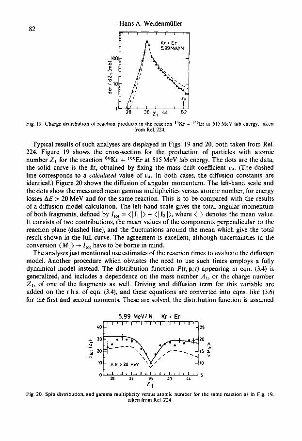
82
r~ E
r,7 "1o " ~ 1 0 b
Hans A. Weidenm011er
-- i I I I I 1 i
N
I t / , 1 1 i I 28 36 Z1 4/. 52
Fig. 19. Charge distribution of reaction products in the reaction a4Kr + t6*Er at 515 MeV lab energy, taken from Ref. 224.
Typical results of such analyses are displayed in Figs. 19 and 20, both taken from Ref. 224. Figure 19 shows the cross-section for the production of particles with atomic number Zt for the reaction S6Kr + t66Er at 515 MeV lab energy. The dots are the data, the solid curve is the fit, obtained by fixing the mass drift coefficient vA. (The dashed line corresponds to a calculated value of oA. In both cases, the diffusion constants are identical.) Figure 20 shows the diffusion of angular momentum. The left-hand scale and the dots show the measured mean gamma multiplicities versus atomic number, for energy losses AE > 20 MeV and for the same reaction. This is to be compared with the results of a diffusion model calculation. The left-hand scale gives the total angular momentum of both fragments, defined by/tot = (1 It J) + (112 J), where ( ) denotes the mean value. It consists of two contributions, the mean values of the components perpendicular to the reaction plane (dashed line), and the fluctuations around the mean which give the total result shown in the full curve. The agreement is excellent, although uncertainties in the conversion (Mr) --, -/tot have to be borne in mind.
The analyses just mentioned use estimates of the reaction times to evaluate the diffusion model. Another procedure which obviates the need to use such times employs a fully dynamical model instead. The distribution function P(r,p;t) appearing in eqn. (3.4) is generalized, and includes a dependence on the mass number At, or the charge number Zt, of one of the fragments as well. Driving and diffusion term for this variable are added on the r.h.s, of eqn. (3.4), and these equations are converted into eqns. like (3.6) for the first and second moments. These are solved, the distribution function is assumed
5.99 MeW N Kr ÷ Er , l , I , I , I , I v I v I v I , 1 ,
~0 - 25
- - 30 ~ - . - ' m ~ T ~ , ~ ~ 2O
"6 20 V
10 I0
0 , f , 1 , I , I , I , I , I , I ~. J j 5 28 32 36 ~0 4/.
Z1 Fig. 20. Spin distribution, and gamma multiplicity versus atomic number for the same reaction as in Fig. 19,
taken from Ref. 224.
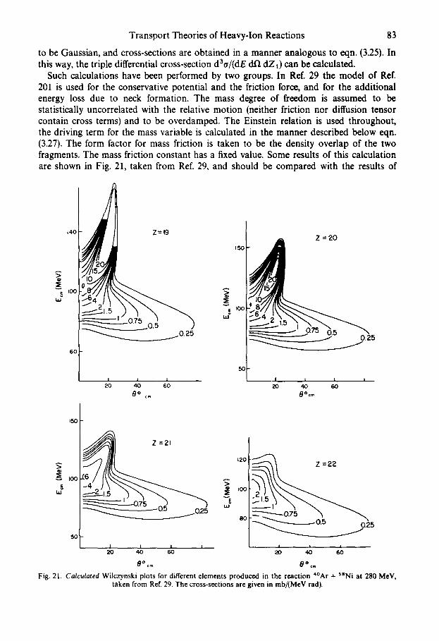
Transport Theories of Heavy-Ion Reactions 83
to be Gaussian, and cross-sections are obtained in a manner analogous to eqn. (3.25). In this way, the triple differential cross-section datr/(dE dr) d Z 0 can be calculated.
Such calculations have been performed by two groups. In Ref. 29 the model of Ref. 201 is used for the conservative potential and the friction force, and for the additional energy loss due to neck formation. The mass degree of freedom is assumed to be statistically uncorrelated with the relative motion (neither friction nor diffusion tensor contain cross terms) and to be overdamped. The Einstein relation is used throughout, the driving term for the mass variable is calculated in the manner described below eqn. (3.27). The form factor for mass friction is taken to be the density overlap of the two fragments. The mass friction constant has a fixed value. Some results of this calculation are shown in Fig. 21, taken from Ref. 29, and should be compared with the results of
~ 4 0 I ~ Z=I9
60 1 I l I
20 40 60 ~ o cm
I 150
? -- 0¢~
I03
501 I l l
20 40 60 ~Ocra
150
,., ~__~_~._2"L~ ~ \ ~
i ~ ~v.~ .025
50 | I I I I
20 40 60
8° cm
I.lJ
120
I00
80
Z =22
I i i -- 2O 40 60
~°¢m
Fig. 21. Calculated Wilczynski plots for different elements produced in the reaction 4°Ar + SaNi at 280 MeV, taken from Ref. 29. The cross-sections are given in mb/(MeV rad).
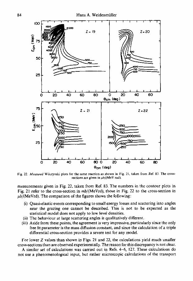
Hans A. Weidenm~iller
I I 1 I 1 I I I I I I00
75
!
75
84
W
25
i 0
I i i I I I I I i 0 80 0 20 40 60
ecru (c~) ! ! i
I 1 I I I t
20 40 60
I I r i i I
Z= 21
5O
I i I i I i
2O 40 6O
1 I I I I I
1
Z-22
I ! I 1 1 I I J 80 0 20 40 60
Oem ((leg)
I
80
Fig. 22. Measured Wilczynski plots for the same reaction as shown in Fig. 21, taken from Ref. 83. The cross- sections are given in/~b/(MeV rad).
measurements given in Fig. 22, taken from Ref. 83. The numbers in the contour plots in Fig. 21 refer to the cross-section in mb/(MeVrd), those in Fig. 22 to the cross-section in pb/(MeVrd). The comparison of the figures shows the following:
(i) Quasi-elastic events corresponding to small energy losses and scattering into angles near the grazing one cannot be described. This is not to be expected as the statistical model does not apply to low level densities.
(ii) The behaviour at large scattering angles is qualitatively different. (iii) Aside from these points, the agreement is very impressive, particularly since the only
free fit parameter is the mass diffusion constant, and since the calculation of a triple differential cross-section provides a severe test for any model.
For lower Z values than shown in Figs. 21 and 22, the calculations yield much smaller cross-sections than are observed experimentally. The reason for this discrepancy is not clear.
A similar set of calculations was carried out in Refs. 4-6, 127. These calculations do not use a phenomenological input, but rather microscopic calculations of the transport
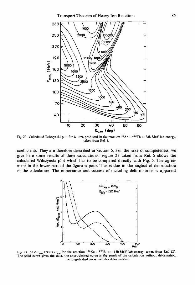
Transport Theories of Heavy-Ion Reactions
280
85
250
220
190
~" 160
E u.~ 130
100
70
40
10 20 30 40 50 60 Oc.m. (deg)
Fig. 23. Calculated Wilczynski plot for K ions produced in the reaction 4°Ar + 232Th at 388 MeV lab energy, taken from Ref. 5.
coefficients. They are therefore described in Section 5. For the sake of completeness, we give here some results of these calculations. Figure 23 taken from Ref. 5 shows the calculated Wilczynski plot which has to be compared directly with Fig. 5. The agree- ment in the lower part of the figure is poor. This is due to the neglect of deformation in the calculation. The importance and success of including deformations is apparent
161TS--S~ I I \ ' \ 136Xe + L:'OeBi II \ \ E lab=ll30 MeV
\ "
\ \
-0 I00 200 300 400 " 500 MeV
Fig. 24. da/dElo ~ versus E~o . for the reaction ~6Xe + 2°9Bi at I130 MeV lab energy, taken from Ref. 127. The solid curve gives the data, the short-dashed curve is the result of the calculation without deformation,
the long-dashed curve includes deformation.
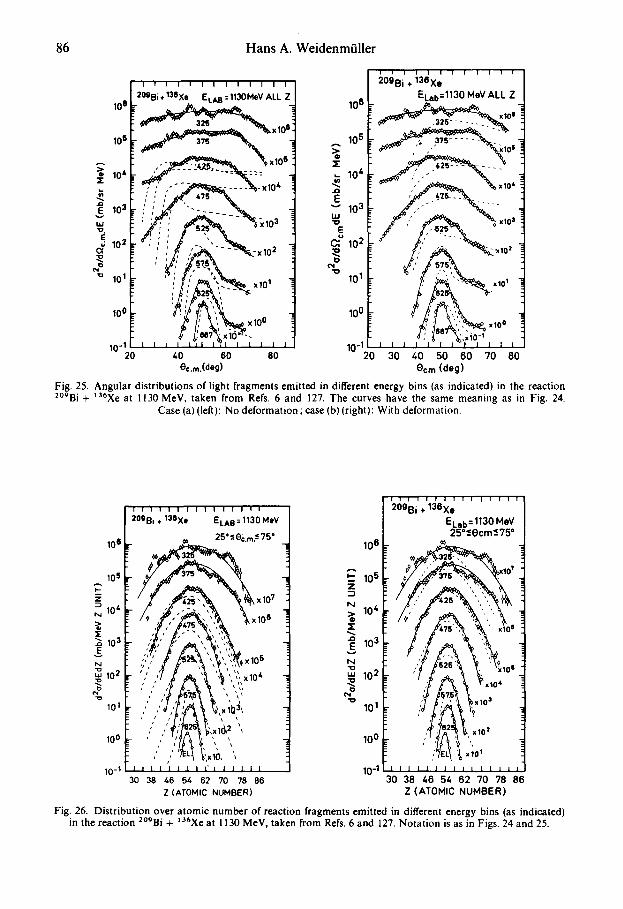
86 Hans A. Weidenmiiller
I I V I 1 I I I I I I I I I I
/2°9Bi + 130Xe EL~B = 1130MeV ALL z l
~ , . - ~ \ x ~ O ~
10, / j
lO, e l / ! I..:'.._'.~=, ,
100 r",~ I" ~, 'x ~ = : i00 ~o_~ , , , ,~ ,~ ,7" ,%'" , ; , , ,
20 40 60 80 e©.m.(deg)
106
105
,. 104
E • .-- 103 LU
E ( ~ 10 2
J • o 101
100
10-1 20
i i i i I I l i I I i i
209Bi . 138Xe ELab=1130 MeV ALL Z
30 40 50 60 70 80 Ocm (deg)
Fig. 25. Angular distributions of light fragments emitted in different energy bins (as indicated) in the reaction 2°9Bi + 136Xe at 1130 MeV, taken from Refs. 6 and 127. The curves have the same meaning as in Fig. 24.
Case (a) (left): No deformation ; case (b) (right): With deformation.
1o 6
105 p-
N 1 0 4
>~
E l 0
,,, 102
¢ lO!
1oo
I 0 - I
i I i I I I I I I I I I I I
2 0 9 B i . 1 3 8 X e E L A O = 1 1 3 0 M e V
U, 25' s e~.m.": 75"
, f .f~._~.,~ ~,x,o, : xl0 "
t i J • ~ h 4 -...
, i i ,, x "
• 1'I i I' f ',
30 38 46 54 62 70 78 86 Z (ATOMIC NUMBER)
i i i i I I i i i I I I 1
209Bi + 136X e ELab = 1130 NeV 25*_cecm~_75 *
108 <0
10, f ?2 \ \ " "t 12 \ \ lO 2
101 . , J , , /~ '~ , ~x 10'
,'TEL / ~ x , o ' 10-1 I I I l I I I I I, I I I I
30 38 46 54 62 70 78 86 Z (ATOMIC NUMBER)
Fig. 26. Distribution over atomic number of reaction fragments emitted in different energy bins (as indicated) in the reaction 2°9Bi + la6Xe at 1130 MeV, taken from Refs. 6 and 127. Notation is as in Figs. 24 and 25.
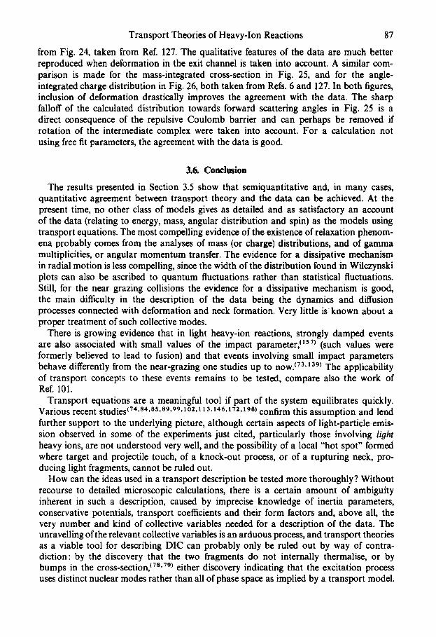
Transport Theories of Heavy-Ion Reactions 87
from Fig. 24, taken from Ref. 127. The qualitative features of the data are much better reproduced when deformation in the exit channel is taken into account. A similar com- parison is made for the mass-integrated cross-section in Fig. 25, and for the angle- integrated charge distribution in Fig. 26, both taken from Refs. 6 and 127. In both figures, inclusion of deformation drastically improves the agreement with the data. The sharp falloff of the calculated distribution towards forward scattering angles in Fig. 25 is a direct consequence of the repulsive Coulomb barrier and can perhaps be removed if rotation of the intermediate complex were taken into account. For a calculation not using free fit parameters, the agreement with the data is good.
3.6. Conclusion
The results presented in Section 3.5 show that semiquantitative and, in many cases, quantitative agreement between transport theory and the data can be achieved. At the present time, no other class of models gives as detailed and as satisfactory an account of the data (relating to energy, mass, angular distribution and spin) as the models using transport equations. The most compelling evidence of the existence of relaxation phenom- ena probably comes from the analyses of mass (or charge) distributions, and of gamma multiplicities, or angular momentum transfer. The evidence for a dissipative mechanism in radial motion is less compelling, since the width of the distribution found in Wilczynski plots can also be ascribed to quantum fluctuations rather than statistical fluctuations. Still, for the near grazing collisions the evidence for a dissipative mechanism is good, the main difficulty in the description of the data being the dynamics and diffusion processes connected with deformation and neck formation. Very little is known about a proper treatment of such collective modes.
There is growing evidence that in light heavy-ion reactions, strongly damped events are also associated with small values of the impact parameter, ~ls~ (such values were formerly believed to lead to fusion) and that events involving small impact parameters behave differently from the near-grazing one studies up to now. ~73" 139~ The applicability of transport concepts to these events remains to be tested, compare also the work of Ref. 101.
Transport equations are a meaningful tool if part of the system equilibrates quickly. Various recent s t u d i e s (74'84'85"89'99' 102,113,146, t 72.190) confirm this assumption and lend further support to the underlying picture, although certain aspects of light-particle emis- sion observed in some of the experiments just cited, particularly those involving light heavy ions, are not understood very well, and the possibility of a local "hot spot" formed where target and projectile touch, of a knock-out process, or of a rupturing neck, pro- ducing light fragments, cannot be ruled out.
How can the ideas used in a transport description be tested more thoroughly? Without recourse to detailed microscopic calculations, there is a certain amount of ambiguity inherent in such a description, caused by imprecise knowledge of inertia parameters, conservative potentials, transport coefficients and their form factors and, above all, the very number and kind of collective variables needed for a description of the data. The unravelling of the relevant collective variables is an arduous process, and transport theories as a viable tool for describing DIC can probably only be ruled out by way of contra- diction: by the discovery that the two fragments do not internally thermalise, or by bumps in the cross-section, (7a'79) either discovery indicating that the excitation process uses distinct nuclear modes rather than all of phase space as implied by a transport model.
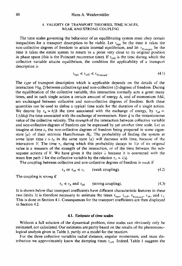
88 Hans A. WeidenmiJller
4. VALIDITY OF TRANSPORT THEORIES, TIME SCALES, WEAK AND STRONG COUPLING
The time scales governing the behaviour of an equilibrating system must obey certain inequalities for a transport description to be viable. Let requ be the time it takes the non-collective degrees of freedom to attain internal equilibrium, and let ZPoincarc be the time it takes the entire system to return to a point very close to its original position in phase space (this is the Poincar6 recurrence time). If ZcoH is the time during which the collective variable attains equilibrium, the condition for applicability of a transport description is
req u ,~ Tcoll ~ TPoincare. (4 .1)
The type of transport description which is applicable depends on the details of the interaction V(q, ~) between collective (q) and non-collective (~) degrees of freedom. During the equilibration of the collective variable, this interaction normally acts a great many times, and in each single action a certain amount of energy A, and of momentum hAk, are exchanged between collective and non-collective degrees of freedom. Both these quantities can be used to define a typical time scale for the duration of a single action. We denote by za = h/A the time associated with the exchange of energy, by rak----- 1/(Ak~) the time associated with the exchange of momentum. Here ~ is the instantaneous value of the collective velocity. The strength of the interaction between collective variable and non-collective degrees of freedom can be expressed by yet another time scale. Let us imagine at time to the non-collective degrees of freedom being prepared in some eigen- state la> of their intrinsic Hamiltonian Ho. The probability of finding the system at some later time t > to in the same state [a) will decrease with time, because of the interaction V. The time r~. during which this probability decays to I/e of its original value is a measure of the strength of the interaction, or of the time between the sub- sequent actions of V. We have given it the index 2 because it is connected with the mean free path 2 for the collective variable by the relation r~. = 2/9.
The coupling between collective and non-collective degrees of freedom is weak if
ra or Zak ~. Z;. (weak coupling). (4.2)
The coupling is strong if
rz ,~ r~ and "CAR (strong coupling). (4.3)
It is shown below that transport coefficients have different characteristic features in these two limits. It is therefore necessary to estimate the times "t'eqo, Tcoll , Tpoincare , TAk , and r;.. This is done in Section 4.1. Consequences for the transport coefficients are then displayed in Section 4.2.
4.1. Estimate of time scales
Without a full solution of the dynamical problem, time scales can obviously only be estimated, not calculated. Our estimates are partly based on the results of the phenomeno- logical analysis given in Table 1, partly on a model for the reaction.
For the three collective variables radial distance, angular momentum, and mass dis- tribution we approximately know the damping times rc,,ll. Indeed, Table 1 suggests the
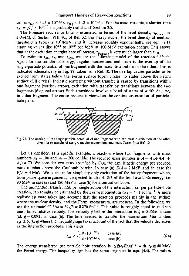
Transport Theories of Heavy-Ion Reactions 89
values rrad "" 3..5 x 10 -22 S, Tang ~ 1..2 X 10 -2t S. For the mass variable, a shorter time zA, = y J-: "-- 10 -22 s is probably realistic, cf. Section 3.5.
The Poincar~ recurrence time is estimated in terms of the level density, TPoinca,~ ~. 2nhp(E), cf. Section VIII 7C, of Ref. 32. For heavy nuclei, the level density at neutron threshold is typically 10S/MeV, and it increases roughly exponentially, see eqn. (2.1), attaining values like l 0 ta to 1020 per MeV at 100 MeV excitation energy. This shows that at the excitation energies here of interest, Tpoincare is very much larger than Zoo,.
To estimate rAk, ~ , and rcqu, we use the following model of the r e a c t i o n . (9 , tS ' t23)
Agent for the transfer of energy, angular momentum, and mass is the overlap of the single-particle potential of one fragment with the mass distribution of the other. This is indicated schematically in Fig. 27, taken from Ref. 10. The overlap causes particles to be excited from states below the Fermi surface (open circles) to states above the Fermi surface (full circles). Inelastic scattering without transfer is caused by transitions within one fragment (vertical arrow), excitation with transfer by transitions between the two fragments (diagonal arrow). Such transitions involve a band of states of width Aet, Ae2 in either fragment. The entire process is viewed as the continuous creation of particle- hole pairs.
Fig. 27. The overlap of the single-particle potential of one fragment with the mass distribution of the other gives rise to transfer of energy, angular momentum, and mass. Taken from Ref. 10.
Let us consider, as a specific example, a reaction where two fragments with mass numbers At = 100 and A2 = 200 collide. The reduced mass number is A = AtA2/(At + A2) = 70. We consider two cases specified by E/A, the c.m. kinetic energy per reduced mass number above the Coulomb barrier. In case (a) E/A = 2 MeV and in case (b) E/A = 4 MeV. We consider for simplicity only excitation of the heavy fragment which, from phase space arguments, is expected to absorb 2/3 of the total available energy, i.e. 90 MeV in case (a) and 180 MeV in case (b) for a central collision.
The momentum transfer hAk per single action of the interaction, i.e. per particle-hole creation, can roughly be estimated by the Fermi momentum hkr = h. 1.36 fm- t. A more realistic estimate takes into account that the reaction proceeds mainly in the surface where the nuclear density, and the Fermi momentum, are reduced. In the following, we use the estimate ~ta~ hAk = hkv/5 = 0.27h fm - t . This value is roughly equal to nucleon mass times relative velocity. The velocity ~ before the interaction is ~ = 0.066c in case (a), t~ = 0.093c in case (b). The time needed to transfer the momentum hAk is thus rak > 5/(kr~) where the inequality sign takes account of the fact that the velocity decreases as the interaction proceeds. This yields
1.9.10 -22 s case (a), r~k > (4.4)
= 1.4" 10 -22 s case (b).
The energy transferred per particle-hole creation is <~(erE/A) t/2 with eF ~ 40 MeV the Fermi energy. The inequality sign has the same origin as in eqn. (4.4). The values
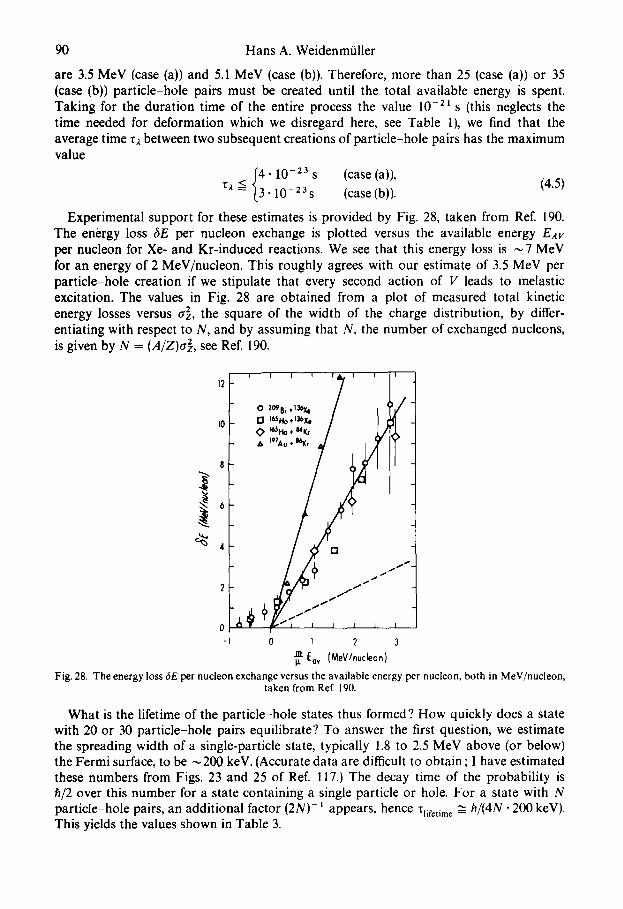
90 Hans A. Weidenmiiller
are 3.5 MeV (case (a)) and 5.1 MeV (case (b)). Therefore, more than 25 (case (a)) or 35 (case (b)) particle-hole pairs must be created until the total available energy is spent. Taking for the duration time of the entire process the value 10 -21 s (this neglects the time needed for deformation which we disregard here, see Table 1), we find that the average time za between two subsequent creations of particle-hole pairs has the maximum value
r~ < t43" 10-23 s (case (a,,' (4.5, = • 10-23S (case (b)).
Experimental support for these estimates is provided by Fig. 28, taken from Ref. 190. The energy loss fiE per nucleon exchange is plotted versus the available energy E,4v per nucleon for Xe- and Kr-induced reactions. We see that this energy loss is ~ 7 MeV for an energy of 2 MeV/nucleon. This roughly agrees with our estimate of 3.5 MeV per particle-hole creation if we stipulate that every second action of V leads to inelastic excitation. The values in Fig. 28 are obtained from a plot of measured total kinetic energy losses versus tr 2, the square of the width of the charge distribution, by differ- entiating with respect to N, and by assuming that N, the number of exchanged nucleons, is given by N = (A/Z)tr 2, see Ref. 190.
I I I I I A
o 2O9Bi + l ~ / [:! I~Ho ,,'~'Xe /
& 197Au, 16~ /
6 Q '
4
i " s I ~ ' s
o ' "" ,
-I 0 ~ 2 3 m Eo v (MeV/nucleon) Is.
Fig. 28. The energy loss fie per nucleon exchange versus the available energy per nucleon, both in MeV/nucleon, taken from Ref. 190.
What is the lifetime of the particle-hole states thus formed? How quickly does a state with 20 or 30 particle-hole pairs equilibrate? To answer the first question, we estimate the spreading width of a single-particle state, typically 1.8 to 2.5 MeV above (or below) the Fermi surface, to be ~200 keV. (Accurate data are difficult to obtain ; I have estimated these numbers from Figs. 23 and 25 of Ref. 117.) The decay time of the probability is h/2 over this number for a state containing a single particle or hole. For a state with N particle-hole pairs, an additional factor (2N)- ~ appears, hence Tlifetime ~ h/(4N" 200 keV). This yields the values shown in Table 3.
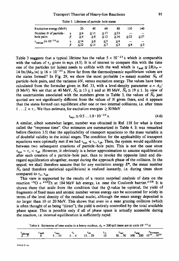
Transport Theories of Heavy-Ion Reactions
Table 3. Lifetimes of particle-hole states
Excitation energy (MeV) 20 40 60 80 110 140
Number N of particle- a _~ 6 _~ 11 _~ 17 ~ 23 - - - - hole pairs // _~4 2 8 ~ 12 ~ 16 _~22 >27
~l,fetim¢ (in 10-2s s) a ~14 ~8 ~ 5 ~ 4 - - -- ~22 ~11 < 7 ~ 5 ~ 4 ~ 3
91
Table 3 suggests that a typical lifetime has the value 5 x 10 -23 s which is comparable with the values of z~ given in eqn. (4.5). It is of interest to compare this with the time one of the particles (or holes) needs to collide with the wall which is ¢wall ~ 2R/vr = 14 fm/(hkF/m) ~ 16 x 10 -23 s. How far from the thermodynamic equilibrium values are the states formed? In Fig. 29, we show the most probable (= mean) number No of particle-hole pairs, and the variance 6N, versus excitation energy. The values have been calculated from the formulae given in Ref. 33, with a level-density parameter a = A2/ (8 MeV). We see that at 40 MeV, /Vo - 13 + 1 and at 80 MeV, No = 19:1: I. In view of the uncertainties associated with the numbers given in Table 3, the values of No just quoted are not significantly different from' the values of N given there, and it appears that the states formed can equilibrate aRer one or two internal collisions, i.e. after times 1 . . . 2 x z:. We thus estimate, for excitation energies ~> 30 MeV
~equ ---- 0.5... 1.0.10 -22 s. (4.6)
A similar, albeit somewhat larger, number was obtained in Ref. 118 for what is there called the "response time". Our estimates are summarized in Table 4. It was remarked before (Section 3.5) that the applicability of transport equations to the mass variable is of doubtful validity in the initial stages. The condition for the applicability of transport equations were optimally met if we had ¢cqu '~ z~, T~. Then, the system would equilibrate between two subsequent creations of particle-hole pairs. This is not the case since Teq u '~ l",;. < "OAk. However, it obviously is a better approximation to assume equilibration after each creation of a particle-hole pair, than to invoke the opposite limit and dis- regard equilibration altogether, except during the approach phase of the collision. In the sequel, we shall therefore assume that for any excitation energy E*, the mean number No (and therefore statistical equilibrium) is realised instantly, i.e. during times short compared to ~ , z~.
This view is supported by the results of a recent surprisal analysis of data on the reaction t60 + 232Th at 104 MeV lab energy, i.e. near the Coulomb barrier. "38) It is shown there that aside from the condition that the Q-value be optimal, the yield of fragments of fixed mass and atomic number versus energy can be accounted for solely in terms of the level density of the residual nuclei, although the mean energy deposited is no larger than 10 or 20 MeV. This shows that even in a near grazing collision (which is often thought of as being "direct"), the yield is entirely controlled by the total available phase space. This is possible only if all of phase space is actually accessible during the reaction, i.e. internal equilibration is sufficiently rapid.
Table 4. Estimates of time scales in a heavy nucleus, A, = 200 (all times are in units 10- 23 s)
8 5...10 3...4 15...20 I0 30... 50 I O0 lOl°... I02°
P.P.N.P.3~
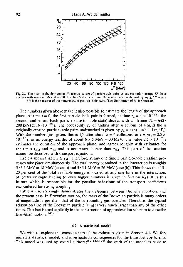
Hans A. WeidenmiJller
' I ' I ' I ' I I I I l ~ I ' I No 28
24
20
16
12
8
4
92
, I , I ~ I ~ I , I , I J I t I
20 40 60 80 100 120 140 160 E*(MeV)
Fig. 29. The most probable number No (centre curve) of particle-hole pairs versus excitation energy E* for a nucleus with mass number A = 200. The hatched area around the centre curve is defined by No + t~N where
fiN is the variance of the number No of particle-hole pairs. (The distribution of No is Gaussian.)
The numbers given above make it also possible to estimate the length of the approach phase. At time t = 0, the first particle-hole pair is formed, at time r~. = 4 x 10 -23 s the second, and so on. Each particle state (or hole state) decays with a lifetime To = hi(2. 200 keV) ~ 16" 10 -22 s. The probability p, of finding after n actions of V(q, ~) the n originally created particle-hole pairs undisturbed is given by p, = e x p ( - n ( n + 1)zffTo). With the numbers just given, this is l/e after about n = 6 collisions, or t = nz~ = 2.5 x 10 -22 s, or an energy transfer of about 6 x 5 MeV = 30 MeV. The value 2.5 x 10 -22 s estimates the duration of the approach phase, and agrees roughly with estimates for the times rN/z and ZA,, and is not much shorter than rrad. This part of the reaction cannot be described with transport equations.
Table 4 shows that 5~ ~ ZAk. Therefore, at any one time 5 particle-hole creation pro- cesses take place simultaneously. The total energy contained in the interaction is roughly 5 .3 .5 MeV = 18 MeV (case (a)) and 5" 5.1 MeV = 26 MeV (case (b)). This shows that 15- 20 per cent of the total available energy is located at any one time in the interaction. (A better estimate leading to even higher numbers is given in Section 4.2). It is this feature which is responsible for the peculiar behaviour of the transport coefficients encountered for strong coupling.
Table 4 also strikingly demonstrates the difference between Brownian motion, and the present case. In Brownian motion, the mass of the Brownian particle is many orders of magnitude larger than that of the surrounding gas particles. Therefore, the typical relaxation time of the Brownian particle (rcoH) is very much larger than any of the other times. This fact is used explicitly in the construction of approximation schemes to describe Brownian motion. (~ 45)
4.2. A statistical model
We wish to explore the consequences of the estimates given in Section 4.1. We for- mulate a statistical model, and investigate its consequences for the transport coefficients. This model was used by several authors; (53'123't29) the spirit of the model is basic to
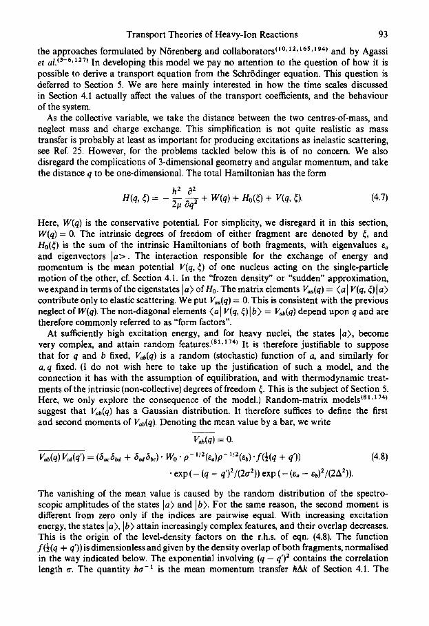
Transport Theories of Heavy-Ion Reactions 93
the approaches formulated by Nfrenberg and collaborators t~ o, 12.165, ~ 9+~ and by Agassi et al. <3-6'127) In developing this model we pay no attention to the question of how it is possible to derive a transport equation from the Schr6dinger equation. This question is deferred to Section 5. We are here mainly interested in how the time scales discussed in Section 4.1 actually affect the values of the transport coefficients, and the behaviour of the system.
As the collective variable, we take the distance between the two centres-of-mass, and neglect mass and charge exchange. This simplification is not quite realistic as mass transfer is probably at least as important for producing excitations as inelastic scattering, see Ref. 25. However, for the problems tackled below this is of no concern. We also disregard the complications of 3-dimensional geometry and angular momentum, and take the distance q to be one-dimensional. The total Hamiltonian has the form
h 2 t3 2 H(q, ~) - 2~ t3q 2 + W(q) + Ho(¢) + V(q, ~). (4.7)
Here, W(q) is the conservative potential. For simplicity, we disregard it in this section, W(q) = 0. The intrinsic degrees of freedom of either fragment are denoted by ~, and Ho(O is the sum of the intrinsic Hamiltonians of both fragments, with eigenvalues eo and eigenvectors la>. The interaction responsible for the exchange of energy and momentum is the mean potential V(q, ~) of one nucleus acting on the single-particle motion of the other, cf. Section 4.1. In the "frozen density" or "sudden" approximation, we expand in terms of the eigenstates l a) of Ho. The matrix elements V,~(q) = (a I V(q, ~)1 a) contribute only to elastic scattering. We put V,~(q) = 0. This is consistent with the previous neglect of W(q). The non-diagonal elements (a I V(q, ~)lb) = V,b(q) depend upon q and are therefore commonly referred to as "form factors".
At sufficiently high excitation energy, and for heavy nuclei, the states la), become very complex, and attain random features, t8~'17+~ It is therefore justifiable to suppose that for q and b fixed, V~(q) is a random (stochastic) function of a, and similarly for a, q fixed. (I do not wish here to take up the justification of such a model, and the connection it has with the assumption of equilibration, and with thermodynamic treat- ments of the intrinsic (non-collective) degrees of freedom ~. This is the subject of Section 5. Here, we only explore the consequence of the model.) Random-matrix models t a t ' t ~ suggest that Vob(q) has a Gaussian distribution. It therefore suffices to define the first and second moments of V,b(q). Denoting the mean value by a bar, we write
V,~(q) = O.
V~(q) V,j(q') = ( ~ , 6 ~ + tS,~b~) " Wo " p - l/2(ea)p- 1/2(~b)"f(½(q + q')) (4.8)
• exp(-- (q -- q')2/(2tr2)) exp (-- (e° -- eb)2/(2A2)).
The vanishing of the mean value is caused by the random distribution of the spectro- scopic amplitudes of the states la) and Ib). For the same reason, the second moment is different from zero only if the indices are pairwise equal. With increasing excitation energy, the states la), Ib) attain increasingly complex features, and their overlap decreases. This is the origin of the level-density factors on the r.h.s, of eqn. (4.8). The function f(½(q + q')) is dimensionless and given by the density overlap of both fragments, normalised in the way indicated below. The exponential involving (q - q,)2 contains the correlation length a. The quantity ha-~ is the mean momentum transfer hAk of Section 4.1. The
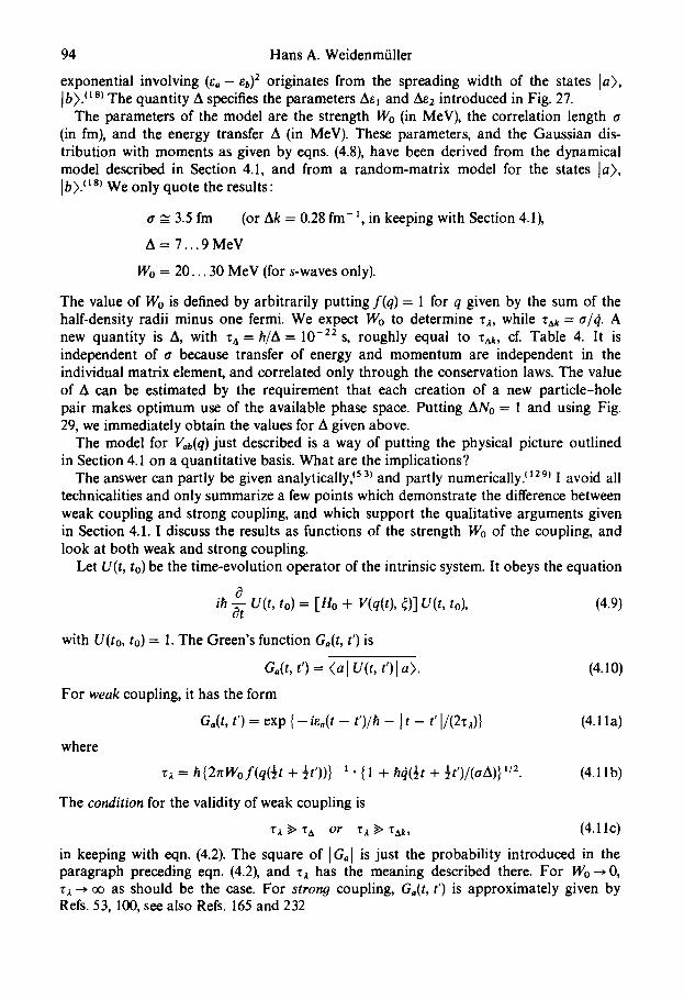
94 Hans A. Weidenmfiller
exponential involving (Ea- eb) 2 originates from the spreading width of the states la>, [b).tl 8~ The quantity A specifies the parameters Ae~ and Ae2 introduced in Fig. 27.
The parameters of the model are the strength Wo (in MeV), the correlation length tr (in fm), and the energy transfer A (in MeV). These parameters, and the Gaussian dis- tribution with moments as given by eqns. (4.8), have been derived from the dynamical model described in Section 4.1, and from a random-matrix model for the states la>, [b). ~ta~ We only quote the results:
tr ~ 3.5 fm (or Ak = 0.28 fm- i, in keeping with Section 4.1),
A = 7 . . . 9 MeV
Wo = 20.. . 30 MeV (for s-waves only).
The value of I41o is defined by arbitrarily putting f (q) = 1 for q given by the sum of the half-density radii minus one fermi. We expect Wo to determine ra, while z~k = a/4. A new quantity is A, with Ta = h/A = 10 -22 s, roughly equal to Zak, cf. Table 4. It is independent of tr because transfer of energy and momentum are independent in the individual matrix element, and correlated only through the conservation laws. The value of A can be estimated by the requirement that each creation of a new particle-hole pair makes optimum use of the available phase space. Putting ANo = 1 and using Fig. 29, we immediately obtain the values for A given above.
The model for V~(q) just described is a way of putting the physical picture outlined in Section 4.1 on a quantitative basis. What are the implications?
The answer can partly be given analytically, ~53~ and partly numerically, t 129~ I avoid all technicalities and only summarize a few points which demonstrate the difference between weak coupling and strong coupling, and which support the qualitative arguments given in Section 4.1. I discuss the results as functions of the strength Wo of the coupling, and look at both weak and strong coupling.
Let U(t, to) be the time-evolution operator of the intrinsic system. It obeys the equation
d ih -~ U(t, to) = [-Ho + V(q(t), 0 ] U(t, to), (4.9)
with U(to, to) = 1. The Green's function Ga(t, t') is
Go(t, t') = <a[ U(t, t ')[a). (4.10)
For weak coupling, it has the form
Go(t, t') = exp { - i e , ( t - t')/h - It - t' I/(2za)} (4.1 la)
where
z a = h { 2nWo f (q(½t + ½t'))}-1 "{1 + h(l(½t + ½t')/(trA)} 1/2 (4.1 lb)
The condition for the validity of weak coupling is
ra~>za or za~>zak, (4.11c)
in keeping with eqn. (4.2). The square of [G,[ is just the probability introduced in the paragraph preceding eqn. (4.2), and zz has the meaning described there. For Wo-~ 0, za ~ oo as should be the case. For strong coupling, G,(t, t') is approximately given by Refs. 53, 100, see also Refs. 165 and 232
Transport Theories of Heavy-Ion Reactions
Go(t, t') ~ exp {-ieo(t - t')/h - (t - t')2/(2z~)}
95
(4.12a)
<Ho> = ~ ebPbo(t, t) -- <a I U+(t, to)HoU(t, to) l a>, b
and the mean value of the total intrinsic Hamiltonian,
(Ho + V) = (a] U+(t, to)(Ho + V)U(t, to)la) (4.15)
= ih -~ ~ p,o(t + ½~, t - ½z) ,=o"
The last equation follows from eqns. (4.13) and (4.9). It is possible to work out analytically the difference between these two mean values. One finds ~53~
<no> = <no + v> + h213/z 2. (4.16)
With 13 ~ (3 MeV)- 1 and za ~ 5 .10 -23 s, we obtain h213/~ ~ 65 MeV. This is an estimate of the energy contained at any one time in the interaction. For a numerical example, see Fig. 36.
It is possible to show that (<Ho + V(q, ¢)> + E~t(q)) is a conserved quantity, equal to the total energy of the system. Here, Er,l(q) is the energy of the relative motion, or the
collective energy, i.e. the expectation value of (h2/21z)O2/Oq 2. Hence, (Ho> may appear only as an auxiliary quantity without interest of its own. This, however, is not the case.
The nuclear temperature, and the parameter 13, are defined in terms of <Ho> by 13 = (kT) - 1 = (a/(Ho>)l/2 with a the level density parameter. This is relevant for the Einstein relation between friction and diffusion coefficient. This relation is shown to have the form of eqn. (3.8),
Dp = 2~k Tl,. (4.17)
However, for strong coupling k T = ((Ho~/a) 1/2 is significantly larger than the nuclear temperature estimated from the energy loss, via the formula ((Eros1- Erel(q))/a) 1/2, cf.
where
z~ = h {nWoAf(q(½t + ½t'))} ,/2 exp ( - (flA)a/16). (4.12b)
The condition for the validity of strong coupling is
z~ ,~ z~ and z~ ,~ zA~, (4.12c)
as stated in eqn. (4.3). The quantity fl in eqn. (4.12b) is the inverse of the nuclear temperature. The approximation h<~/(~rA) <~ 1 has been used.
Using the values Wo = 20 MeV, A = 8 MeV, f = 1, 13 = (3 MeV)- t to calculate T~ from eqns. (4.11b) and (4.12b), and using the inequalities (4.11c) and (4.12c), we find that the strong-coupling limit is realized with a value z~ = 2 x 10 -23 s, in qualitative agreement with the figures given in Table 4.
We now consider the averaged density matrix of the intrinsic system.
pba(t, t') = <bl u(t , to)la)(al u+(t ', to)l b). (4.13)
It is the mean value of the product of two amplitudes, taken at different times t and t'. We define the expectation value of the free intrinsic Hamiltonian,
(4.14)
96 Hans A. Weidenmfiller
eqn. (4.16). This shows that the Einstein relation is actually violated for strong coupling, the diffusion coefficient being 1.3-1.5 times larger than this relation (with a temperature determined from energy conservation) would predict. Illustrative examples for the different behaviour of the expectation values (4.14) and (4.15) may be found in Ref. 129.
The difference between weak and strong coupling is thus well defined. For weak coupling, ~-- . ~ , and eqn. (4.16) shows that the expectation values (4.14) and (4.15) coincide, so that eqn. (4.17) is the usual Einstein relation. For strong coupling, the large amount of energy residing in the interaction leads to a violation of this condition, and to an increase of the diffusion constant over and above the values expected on the basis of the Einstein relation with a temperature calculated via energy conservation.
The reason for this deviation from the Einstein relation lies in the large correlation length, or the small momentum transfer hAk per collision. Indeed, keeping A and Wo fixed and decreasing a, we leave the domain of the validity of condition (4.12c) and enter that of condition (4.11c). There is another area of physics where large correlation lengths occur : in the calculation of transport coefficients near critical points. At a critical point, long-range order is established, and at temperatures right above it, this fact is foreshadowed by the establishment of large correlation lengths. The methods used there to calculate transport coefficients use mode-mode coupling theories, and renormalization group techniques3144o 175) The relationship between these methods, and the ones used in the present context (see Section 5), does not seem to have been investigated.
The results just mentioned can be interpreted in yet another way. ~129~ The short time ra between two subsequent actions of V(q, ~) leads to a short mean free path 2 = ~za, and to a corresponding large momentum uncertainty h6k = h(~z~.)-'. Condition (4.12c) can be put in the form h6k ,> hAk: the momentum uncertainty is large compared to the momentum transfer. This leads to a large uncertainty in the energy, 6E = 2E(fk/k), and
it is this uncertainty which reflects itself in the difference between (Ho) and (Ho + V(q, ~)). The uncertainty is amplified because the large available phase space favours large intrinsic
energies (H0) while no such strong phase space factor acts on the momentum, or the energy, of the collective variable. Phase space manifests itself directly in eqn. (4.16) via the parameter /3. For this reason the behaviour of the system encountered in the strong- coupling limit has been termed "off-shell behaviour". ~129~
In calculating the transport coefficients in the strong-coupling limit, it is obviously not sufficient to only keep track of the instantaneous energy loss of the collective degree(s) of freedom. Two routes are posible: one must either keep a record of the previous history of the system (then the process is non-Markovian), or evaluate the time-evolution of
(Ho) as an independent variable. The latter route increases the number of variables which describe the system but leads to a Markovian problem. It has recently been used successfully. ~1s7~ This reflects a general statement: ~213~ "Whether or not a physical phenomenon constitutes a Markov process depends on the choice of the variables. The task of the physicist is to find the appropriate set of variables in which the process is Markovian."
Can deviations from the Einstein relation such as the one discussed above be detected experimentally? In the realm of heavy-ion physics, I know of no such direct test. The task is surely not an easy one, because the other parameters describing the system (potential, inertia) are not known very precisely. Deriving an unambiguous test is a great challenge.
Our conclusions are based on the simple physical picture developed in Section 4.1 and quantified by eqns. (4.8). Surely this model demonstrates the great importance of a
Transport Theories of Heavy-Ion Reactions 97
thorough discussion of the relevant time scales for any transport-theoretical approach. How general are the conclusions we have drawn? Unfortunately, no other model has been developed and studied in detail comparable to that of Section 4.1. It seems difficult, however, to dramatically alter the time scales given above as long as one remains in a purely stochastic framework.
It has been argued t7°'~2) that the need to consider the strong-coupling limit might be due to the use of the frozen-density, or sudden basis made in eqns. (4.8), and that the choice of an adiabatic basis might reduce the problem to a weak-coupling situation. This, of course, would only be possible if the time-scales estimated in this section would have qualitatively different values in an adiabatic basis. No investigation of this problem appears to have been published. This problem presently is therefore unresolved. The estimation of the relevant time scales should be a challenge to the proponents of a weak- coupling theory in an adiabatic basis.
5. SURVEY OF THE THEORETICAL APPROACHES
As pointed out in Section 3, transport equations differ fundamentally from the Schr6dinger equation. They violate time-reversal invariance, and they describe the time- evolution of a probability distribution, not an amplitude. How is it possible to derive such equations from a microscopic input?
Much about this question can be learned from other fields of physics where transport equations have long been used. At the same time, it is necessary to keep in mind the peculiarities of the nuclear situation.
Generally speaking, a sufficient condition for establishing transport equations is a rapid destruction of phase correlations in the system. This was first recognised by Pauli. t17°~ Such a rapid destruction is expected to come about in any strongly interacting many- body system. Strongly interacting systems are typically systems for which perturbative methods are not applicable. Put in classical terms, the reason for the failure of pertur- bative methods in such systems is the following. Two trajectories of the system which start at two infinitesimally close points in phase space diverge exponentially. Therefore, neither numerical nor analytical methods exist to calculate these trajectories. However, such a calculation would anyway be neither interesting nor desirable, since the slightest perturbation would grossly alter the trajectories. Therefore, an entirely different description is called for, which completely renounces the concept of a trajectory. This is the description developed in classical or quantum-statistical mechanics which emphasises the tendency of such strongly interacting systems to fill all the available phase space, and thus to attain internal equilibrium. In the quantum context, this implies, in particular, a destruc- tion of phase correlations, and a description in terms of probabilities. In the realm of statistical mechanics, powerful techniques for the derivation of transport equations have been developed. ~t19,147,lsS'2t2,231~ A survey of recent theoretical efforts to describe strongly interacting systems may be found in Ref. 176.
In the context of heavy-ion physics, the existing approaches may be classified as follows. The theory of Gross and Kalinowski t2°'9°'93'95'97> emphasises the approach phase of the reaction. According to these authors, 70 per cent of the available energy is transformed into intrinsic excitation during the first 10-22 s of the reaction. The numbers presented in Section 4.1 show that during such times, a transport description is not adequate. Therefore, the authors develop a perturbation-theoretical framework which is based on
98 Hans A. Weidenmiiller
the physical picture described in Section 4.1 : an increasing number of particle-hole pairs is formed in each fragment. A somewhat similar dynamical model has been pursued much further by Glas and Mosel. ta6'aa) These authors use the two-centre shell model to follow the time evolution of the system. Because of computational difficulties, they consider scattering of 160 by ~60, and not of heavier fragments. In this model, energy dissipation is limited by the size of the particle-hole space chosen for the calculation. Their work may be viewed as an effort to follow the evolution of the system as far as is dynamically and computationally possible, starting from the approach phase.
The other approaches use the assumption of rapid internal equilibration of the non- collective degrees of freedom, and thus do not apply to the approach phase of the reaction. Some authors replace the noncollective degrees of freedom by a heat bath of temperature T. This applies to the work by Swiatecki and Randrup and collabora- tors, tag'~vg) to the work of Hofmann, Siemens, and collaborators, "°5'11°) and to the "piston model" of Gross. t93) The density matrix of a heat bath has the form exp{ - f lHol / Trace [exp {-f lHo/] where fl = (KT)-1 and Ho is the Hamiltonian of the noncollective degrees of freedom. This density matrix contains an average over a set of states, and lacks phase correlations between different states, the two ingredients characterising trans- port equations. Thermodynamic averages of the interaction V(q, ~) between collective and noncollective degrees of freedom transfer these properties to the collective variables, and lead to transport equations. Other authors renounce the use of a heat bath, and use instead a statistical hypothesis on the matrix elements of V(q, ~). Such a hypothesis was introduced in eqn. (4.8). It implies that all states in an energy interval between eo and (co + deo) have equal a priori occupation probabilities, and that there are no phase cor- relations between different matrix elements of V(q, ~). Therefore, an average of the density matrix over a sufficiently large number of states l a) (such an average is used in eqn. (4.13)) lacks phase correlations, and has the tendency to fill all available phase space-- i.e. behaves irreversibly. This second approach towards the derivation of transport equation has been mainly used by Ayik, N6renberg, and collaborators, tg'12A65) and by Agassi, Ko and Weidenmiiller. ~a,123) It extends methods and concepts developed pre- viously in the statistical theory of spectra, ~s4'at'~*) in the theory of the optical-model potential and of doorway states, ~s,14°) and of compound and precompound pro- cesses,t2, t2o, 1,9) to the domain of heavy-ion physics.
The underlying physical picture of the excitation process common to most approaches is the one pictorially described in Section 4.1. The mean field of one nucleus produces particle-hole excitations in the other, and the overlap of the two potentials makes nucleon transfer processes possible. Less clear is the answer to the question: which is the agent physically responsible for the loss of phase memory, and thermalisation or randomisation of the noncollective degrees of freedom? It should be borne in mind that the answer to this question is immaterial for the formulation of the theory, since the assumption of thermal equilibrium, or of randomness of matrix elements, obviates the need to specify how the system arranges for these assumptions to be fulfilled. Two schools of thought exist concerning the answer. One school taS) emphasises collisions between the nucleons and the potential walls as the randomising agent which establishes thermal equilibrium in either container (i.e. potential). If the nuclear surface has multipole com- ponents higher than quadrupole, collisions with the wall do, indeed, contribute to randomisation, t3s) In Section 4.1, we estimated the time between two subsequent collisions of a particle, or a hole with the wall by Zwall ~ 1.6 x 10 -22 S. The other school of thought t3~ emphasises the role of nucleon-nucleon collisions as the agent for thermal-
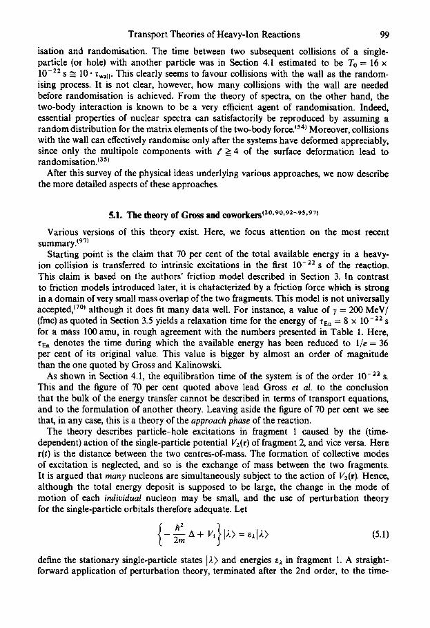
Transport Theories of Heavy-Ion Reactions 99
isation and randomisation. The time between two subsequent collisions of a single- particle (or hole) with another particle was in Section 4.1 estimated to be To = 16 × 10 -22 s --- 10. ~wall. This clearly seems to favour collisions with the wall as the random- ising process. It is not clear, however, how many collisions with the wall are needed before randomisation is achieved. From the theory of spectra, on the other hand, the two-body interaction is known to be a very efficient agent of randomisation. Indeed, essential properties of nuclear spectra can satisfactorily be reproduced by assuming a random distribution for the matrix elements of the two-body force3 s4) Moreover, collisions with the wall can effectively randomise only after the systems have deformed appreciably, since only the multipole Components with t' ___ 4 of the surface deformation lead to randomisation. ~3s~
After this survey of the physical ideas underlying various approaches, we now describe the more detailed aspects of these approaches.
5.1. The theory of Gross and coworkel'$ (20'90'92-95'97)
Various versions of this theory exist. Here, we focus attention on the most recent summary. (97)
Starting point is the claim that 70 per cent of the total available energy in a heavy- ion collision is transferred to intrinsic excitations in the first 10-22 s of the reaction. This claim is based on the authors' friction model described in Section 3. In contrast to friction models introduced later, it is chatacterized by a friction force which is strong in a domain of very small mass overlap of the two fragments. This model is not universally accepted, ~7°~ although it does fit many data well. For instance, a value of ~ = 200 MeV/ (fmc) as quoted in Section 3.5 yields a relaxation time for the energy of ZEn = 8 x 10 -22 S for a mass 100 amu, in rough agreement with the numbers presented in Table 1. Here, TEn denotes the time during which the available energy has been reduced to 1/e = 36 per cent of its original value. This value is bigger by almost an order of magnitude than the one quoted by Gross and Kalinowski.
As shown in Section 4.1, the equilibration time of the system is of the order 10 -22 s. This and the figure of 70 per cent quoted above lead Gross et al. to the conclusion that the bulk of the energy transfer cannot be described in terms of transport equations, and to the formulation of another theory. Leaving aside the figure of 70 per cent we see that, in any case, this is a theory of the approach phase of the reaction.
The theory describes particle-hole excitations in fragment 1 caused by the (time- dependent) action of the single-particle potential V2(r) of fragment 2, and vice versa. Here r(t) is the distance between the two centres-of-mass. The formation of collective modes of excitation is neglected, and so is the exchange of mass between the two fragments. It is argued that many nucleons are simultaneously subject to the action of V2(r). Hence, although the total energy deposit is supposed to be large, the change in the mode of motion of each individual nucleon may be small, and the use of perturbation theory for the single-particle orbitals therefore adequate. Let
t } - • + v l I).> = (5.1)
define the stationary single-particle states 12> and energies ea in fragment 1. A straight- forward application of perturbation theory, terminated after the 2nd order, to the time-
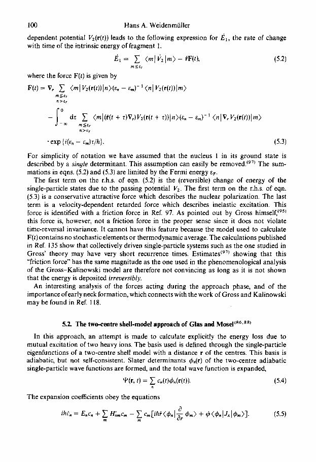
100 Hans A. Weidenmfiller
dependent potential V2(r(t)) leads to the following expression for/~1, the rate of change with time of the intrinsic energy of fragment 1.
/~1 = ~ (ml V2 Im) - eF(t), (5.2)
where the force F(t) is given by
F(t) = V, ~.. (mlV2(r(t))ln)(e, - em)-~<nlVz(r(t))[m) n > £ F
_ f ° dz ~ ~ml ( , ( t+r )V , )V2(r ( t+r ) ) ln ) (e~-e , ) -x(nlV,V2(r(t))[m ~ J - et3 m ~ 8
P1~>8 F
• exp {i(e. - e.m)z/h}. (5.3)
For simplicity of notation we have assumed that the nucleus 1 in its ground state is described by a single determinant. This assumption can easily be removed, t97~ The sum- mations in eqns. (5.2) and (5.3) are limited by the Fermi energy ee.
The first term on the r.h.s, of eqn. (5.2) is the (reversible) change of energy of the single-particle states due to the passing potential V2. The first term on the r.h.s, of eqn. (5.3) is a conservative attractive force which describes the nuclear polarization. The last term is a velocity-dependent retarded force which describes inelastic excitation. This force is identified with a friction force in Ref. 97. As pointed out by Gross himself, t95~ this force is, however, not a friction force in the proper sense since it does not violate time-reversal invariance. It cannot have this feature because the model used to calculate F(t) contains no stochastic elements or thermodynamic average. The calculations published in Ref. 135 show that collectively driven single-particle systems such as the one studied in Gross' theory may have very short recurrence times. Estimates ~97~ showing that this "friction force" has the same magnitude as the one used in the phenomenological analysis of the Gross-Kalinowski model are therefore not convincing as long as it is not shown that the energy is deposited irreversibly.
An interesting analysis of the forces acting during the approach phase, and of the importance of early neck formation, which connects with the work of Gross and Kalinowski may be found in Ref. 118.
5.2. The two-centre shell-model approach of Glas and Mosei ~86'58)
In this approach, an attempt is made to calculate explicitly the energy loss due to mutual excitation of two heavy ions. The basis used is defined through the single-particle eigenfunctions of a two-centre shell model with a distance r of the centres. This basis is adiabatic, but not self-consistent. Slater determinants ~b,(r) of the two-centre adiabatic single-particle wave functions are formed, and the total wave function is expanded,
q~(r, t) = ~ c,(t)qS,(r(t)). (5.4) n
The expansion coefficients obey the equations
ihkn = E~c, + y. H'~c, - y. c , [ i h ~ < ~ [ ~ ~ ,> + ,~<~,lJ~l~,>]. (5.5) m ra
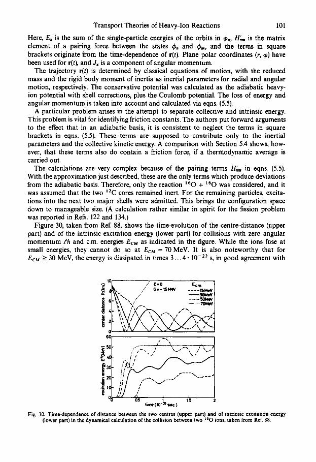
Transport Theories of Heavy-Ion Reactions 101
Here, E, is the sum of the single-particle energies of the orbits in 0,, H~, is the matrix element of a pairing force between the states 0, and Om, and the terms in square brackets originate from the time-dependence of r(t). Plane polar coordinates (r, t#) have been used for r(t), and Jx is a component of angular momentum.
The trajectory r(t) is determined by classical equations of motion, with the reduced mass and the rigid body moment of inertia as inertial parameters for radial and angular motion, respectively. The conservative potential was calculated as the adiabatic heavy- ion potential with shell corrections, plus the Coulomb potential. The loss of energy and angular momentum is taken into account and calculated via eqns. (5.5).
A particular problem arises in the attempt to separate collective and intrinsic energy. This problem is vital for identifying friction constants. The authors put forward arguments to the effect that in an adiabatic basis, it is consistent to neglect the terms in square brackets in eqns. (5.5). These terms are supposed to contribute only to the inertial parameters and the collective kinetic energy. A comparison with Section 5.4 shows, how- ever, that these terms also do contain a friction force, if a thermodynamic average is carried out.
The calculations are very complex because of the pairing terms H~, in eqns. (5.5). With the approximation just described, these are the only terms which produce deviations from the adiabatic basis. Therefore, only the reaction 1~O + ' ° 0 was considered, and it was assumed that the two t2C cores remained inert. For the remaining particles, excita- tions into the next two major shells were admitted. This brings the configuration space down to manageable size. (A calculation rather similar in spirit for the fission problem was reported in Refs. 122 and 134.)
Figure 30, taken from Ref. 88, shows the time-evolution of the centre-distance (upper part) and of the intrinsic excitation energy (lower part) for collisions with zero angular momentum ~'h and c.m. energies EcM as indicated in the figure. While the ions fuse at small energies, they cannot do so at EcM = 70 MeV. It is also noteworthy that for EcM > 30 MeV, the energy is dissipated in times 3 . . . 4 . 10 -22 s, in good agreement with
• "~ I0 t / ~=0 Ecru -- ~ , / " G,-LSMeV . . . . ISl4eV
60
,~so ......""' ........... , ........... ~:"-" ."~.,"--7~,"-':~ ...' / - . , . . , . ,
~30 "t
Cl QS 1 1.5 2 time (10"21 sec )
Fig. 30. Time-dependence of distance between the two centres (upper part) and of intrinsic excitation energy (lower part) in the dynamical calculation of the collision between two '60 ions, taken from Ref. 88.
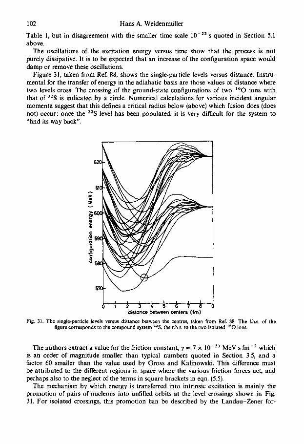
102 Hans A. WeidenmiJller
Table 1, but in disagreement with the smaller time scale 10 -22 s quoted in Section 5.1 above.
The oscillations of the excitation energy versus time show that the process is not purely dissipative. It is to be expected that an increase of the configuration space would damp or remove these oscillations.
Figure 31, taken from Ref. 88, shows the single-particle levels versus distance. Instru- mental for the transfer of energy in the adiabatic basis are those values of distance where two levels cross. The crossing of the ground-state configurations of two ~60 ions with that of 32S is indicated by a circle. Numerical calculations for various incident angular momenta suggest that this defines a critical radius below (above) which fusion does (does not) occur: once the 32S level has been populated, it is very difficult for the system to "find its way back".
0 1 2 3 4 5 6 7 8 9 oistance between centers (fro)
Fig. 31. The single-particle levels versus distance between the centres, taken from Ref. 88. The l.h.s, of the figure corresponds to the compound system 32S, the r.h.s, to the two isolated m60 ions.
The authors extract a value for the friction constant, ~ = 7 x 10 -2a MeV s fm -2 which is an order of magnitude smaller than typical numbers quoted in Section 3.5, and a factor 60 smaller than the value used by Gross and Kalinowski. This difference must be attributed to the different regions in space where the various friction forces act, and perhaps also to the neglect of the terms in square brackets in eqn. (5.5).
The mechanism by which energy is transferred into intrinsic excitation is mainly the promotion of pairs of nucleons into unfilled orbits at the level crossings shown in Fig. 31. For isolated crossings, this promotion tan be described by the Landau-Zener for-
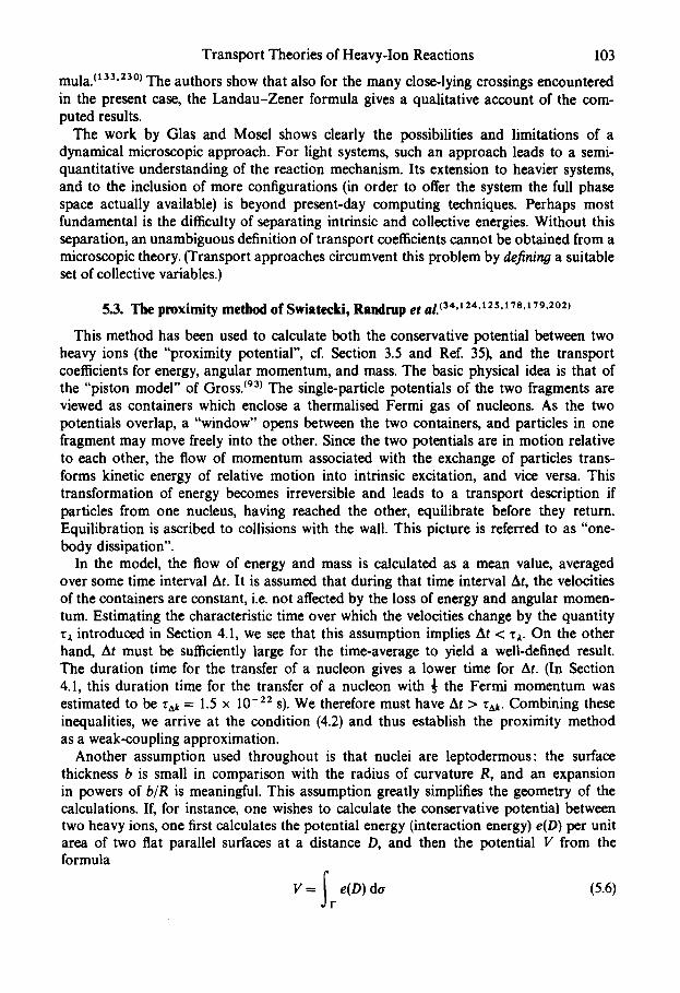
Transport Theories of Heavy-Ion Reactions 103
mula. "33'23°~ The authors show that also for the many close-lying crossings encountered in the present case, the Landau-Zener formula gives a qualitative account of the com- puted results.
The work by Glas and Mosel shows clearly the possibilities and limitations of a dynamical microscopic approach. For light systems, such an approach leads to a semi- quantitative understanding of the reaction mechanism. Its extension to heavier systems, and to the inclusion of more configurations (in order to offer the system the full phase space actually available) is beyond present-day computing techniques. Perhaps most fundamental is the difficulty of separating intrinsic and collective energies. Without this separation, an unambiguous definition of transport coefficients cannot be obtained from a microscopic theory. (Transport approaches circumvent this problem by defining a suitable set of collective variables.)
5.3. The proximity method o f Swiatecki, Randrup e t al. (34' 124., 125.178,179,202)
This method has been used to calculate both the conservative potential between two heavy ions (the "proximity potential", cf. Section 3.5 and Ref. 35), and the transport coefficients for energy, angular momentum, and mass. The basic physical idea is that of the "piston model" of GrossJ 93) The single-particle potentials of the two fragments are viewed as containers which enclose a thermalised Fermi gas of nucleons. As the two potentials overlap, a "window" opens between the two containers, and particles in one fragment may move freely into the other. Since the two potentials are in motion relative to each other, the flow of momentum associated with the exchange of particles trans- forms kinetic energy of relative motion into intrinsic excitation, and vice versa. This transformation of energy becomes irreversible and leads to a transport description if particles from one nucleus, having reached the other, equilibrate before they return. Equilibration is ascribed to collisions with the wall. This picture is referred to as "one- body dissipation".
In the model, the flow of energy and mass is calculated as a mean value, averaged over some time interval At. It is assumed that during that time interval At, the velocities of the containers are constant, i.e. not affected by the loss of energy and angular momen- tum. Estimating the characteristic time over which the velocities change by the quantity • x introduced in Section 4.1, we see that this assumption implies At < z~. On the other hand, At must be sufficiently large for the time-average to yield a well-defined result. The duration time for the transfer of a nucleon gives a lower time for At. (In Section 4.1, this duration time for the transfer of a nucleon with ~: the Fermi momentum was estimated to be ZA~ = 1.5 x 10 -22 s). We therefore must have At > ZAk. Combining these inequalities, we arrive at the condition (4.2) and thus establish the proximity method as a weak-coupling approximation.
Another assumption used throughout is that nuclei are leptodermous: the surface thickness b is small in comparison with the radius of curvature R, and an expansion in powers of b/R is meaningful. This assumption greatly simplifies the geometry of the calculations. If, for instance, one wishes to calculate the conservative potential between two heavy ions, one first calculates the potential energy (interaction energy) e(D) per unit area of two flat parallel surfaces at a distance D, and then the potential V from the formula
= ~ e(D) da (5.6) V d F
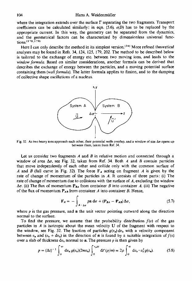
104 Hans A. Weidenmiiller
where the integration extends over the surface F separating the two fragments. Transport coefficients can be calculated similarly: in eqn. (5.6), e(D) has to be replaced by the appropriate current. In this way, the geometry can be separated from the dynamics, and the geometrical factors can be characterized by dimensionless universal func- tions.~ vs.~ 79)
Here I can only describe the method in its simplest version/TM More refined theoretical analyses may be found in Refs. 34, 124, 125, 179, 202. The method to be described below is tailored to the exchange of energy etc. between two moving ions, and leads to the window formula. Based on similar considerations, another formula can be derived that describes the exchange of energy between the particles, and a moving potential surface containing them (wall formula). The latter formula applies to fission, and to the damping of collective shape oscillations of a nucleus.
x,y
Fig. 32. As two heavy ions approach each other, their potential wells overlap, and a window of size Aa opens up between them, taken from Ref. 34.
Let us consider two fragments A and B in relative motion and connected through a window of area Aa, see Fig. 32, taken from Ref. 34. Both A and B contain particles that move independently of each other and collide only with the common surface of A and B (full curve in Fig. 32). The force FA acting on fragment A is given by the rate of change of momentum of the particles in A. It consists of three parts: (i) The rate of change of momentum due to collisions with the surface of A, excluding the window Aa. (ii) The flux of momentum PnA from container B into container A. (iii) The negative of the flux of momentum PAn from container A into container B. Hence,
FA = - ~ pn da + (PnA - PAB)AO', (5.7) J A - AO
where p is the gas pressure, and n the unit vector pointing outward along the direction normal to the surface.
To find the pressure, we assume that the probability distribution f(v) of the gas particles in A is isotropic about the mean velocity U of the fragment with respect to the window, see Fig. 32. The fraction of particles #(vn)dvn with a velocity component between v~ and (v~ + dr,) in the direction of n is found by a suitable integration off(v) over a slab of thickness dr, normal to n. The pressure p is then given by
p = (At)- 1 dr, ,q(v,)(2mt,.) d~ (p/m) = 2p dv," v2ng(v~). (5.8)
Transport Theories of Heavy-Ion Reactions 105
Here, (2my,) is the normal momentum transferred to the wall by each particle of mass m and velocity v,; the number of particles with velocity v, reaching the wall per unit time is
1 I v.ttt -~ jo de~o/m)
with p the mass density. By the same arguments one finds for PnA the expression
P A=j ° dvxvzg(vx)(U±+ W + vzez). (5.9)
Here, the z-axis is chosen normal to the surface Aa and pointing towards B, and ex is the unit vector in z-direction. The velocity W is the velocity of the window with respect to some inertial system. The force FA can now be calculated in a straightforward manner. Assuming that the velocities U, U' and W are small compared to typical nucleon velocities, and keeping only the leading terms, one finds the "window formula"
FA = no" As" (2n I + u~). (5.10)
Here, no = ¼vp (with v the mean velocity) is the static one-sided flux of particles in the gas, and u - U' - U is the velocity of B relative to A. The symbol Ull indicates the com- ponent of u parallel to the normal of the window, while u~ is the component of u in the plane of the window. The force F is a genuine friction force, with the radial friction coefficient given by twice the tangential one. This is because the component of the motion normal to the window affects the rate of exchange of particles, while the parallel one does not.
The formula (5.10) has been derived for a classical gas of particles, and the simplest geometry possible. Naturally, several corrections must be considered. The extension of eqn. (5.10) to complex geometries has been given in Ref. 179. It is based on the proximity approximation, and on the Thomas-Fermi approximation (quasi-classical approximation) for the nucleon motion. Exchange effects have been shown to be negligible. ~3a' 1 ~s~ Quantum effects have been studied in special cases in conjunction with the wall formula; t3a~ it appears that there is at least an order-of-magnitude agreement between the full quantal calculation, and the energy loss predicted by the wall formula if the potential well has a surface deformation with multipolarity ~' > 6. For low t" values (quadrupole and hexa- decupole deformations), the classical motion shows a considerable amount of reversibility which is absent in the energy dissipation predicted by the wall formula.
The friction coefficients given by the window formula have been used in the analyses of some data, 126~ some of the results are shown in Fig. 13a,b. The wall formula has also been applied to fission ;t3a~ it appears that the mean kinetic energies of the fission fragments can be accounted for, cf. also Ref. 202.
In the form given above, the window formula is based upon the assumption of free passage of nucleons through the window. Essentially the same idea has been used by Randrup tlTs~ to calculate the drift and the diffusion coefficients for mass transfer. A rather different approach, based upon a similar physical picture but emphasising the possibility for nucleons to tunnel through a thin potential barrier separating the two fragments leads to results t12a~ which are radically different from those of Randrup. Dynamical studies along the lines of Ref. 25 may be required to resolve this discrepancy. It is not clear whether these observations point to similar deficiencies of the window formula for energy transfer. Finally, we remark again that the wall, and the window, formulae are based upon a weak-coupling approximation. In view of the numbers pre-
106 Hans A. Weidenm~iller
sented in Section 4, it is doubtful whether the limit of weak-coupling is actually applicable, although it may perhaps yield correct order-of-magnitude estimates.
5.4. The "linear response" theory of Hofmann, Siemens et a/. (1°3'1°4'1°6'1°7'11o-1 t 2.1as)
In this theory, the collective degrees of freedom are treated classically, and it is assumed that the equilibration time for the noncollective degrees of freedom is very short compared to the characteristic time over which the collective degrees of freedom change appreciably, Z~qu '~ Z~oll. (The confinement to a classical description of the collective variable can be removed, in principle.) In this section, I present a simplified version of the theory which does not use some of the thermodynamic concepts of the original papers. This simplified version contains the same basic ideas and assumptions as the full-fledged theory. Let q denote the (one-dimensional) collective variable, and let the Hamiltonian have the form of eqn. (4.7), with the notation as explained there.
h 2 82 H(q, ¢) = 2~ 8q 2 + W(q) + Ho(~) + V(q, ~). (5.11)
Treating the collective variable classically, we obtain the following two coupled equations of motion. (Dots indicate time-derivatives.)
l 0v , OW Trace p (5.12a) p/j -- ~q ~-qJ
ih~ = [(/-to + v), p]. (5.12b)
Here, P is the density matrix for the intrinsic degrees of freedom. It obeys eqn. (5.12b) which depends, through K parametrically on q(t). In eqn. (5.12a), the trace over the noncolic~tive degrees of freedom ~ yields a force on q which has to be added to the conservative force - 8W/Sq.
The main assumption of the theory is that at any one time, p is very close to thermal equilibrium. It is then possible to calculate deviations from equilibrium in terms of low- order perturbation theory, using eqn. (5.12b). Substituting the result into eqn. (5.12a), one finds the effective force acting on q(t). In this way one avoids having to solve the coupled equations (5.12) at all times.
What is the perturbation? In our simplified version, we take for it K the full coupling between collective and noncollective degrees of freedom. In the full theory, the interaction V is expanded about some mean value qo, and the difference V(q, ~) - V(qo, ~) is taken as a perturbation. Here, qo is defined as the mean value of q (token over the statistical distribution) taken at time to. Subsequently, the classical path and the behaviour of the system are calculated. The path encompasses a series of points qo(t) around which the perturbation V(q, ~) - V(qo, ~) has been taken into account perturbatively. A more precise definition of these steps is given in Appendix A.
In the interaction representation, defined for any operator 0 by 0 = e x p ( - i H 0 ( t - toffh)O exp ( + iHo(t - to)/h), eqn. (5.12b) has the form
= ( 5 . 1 2 c )
We solve this equation, using first-order perturbation theory, and under the assumption that at time t = to, the system is in equilibrium,
p(to) = exp ( - flHo), frace { exp - (flHo)} = po. (5.13)
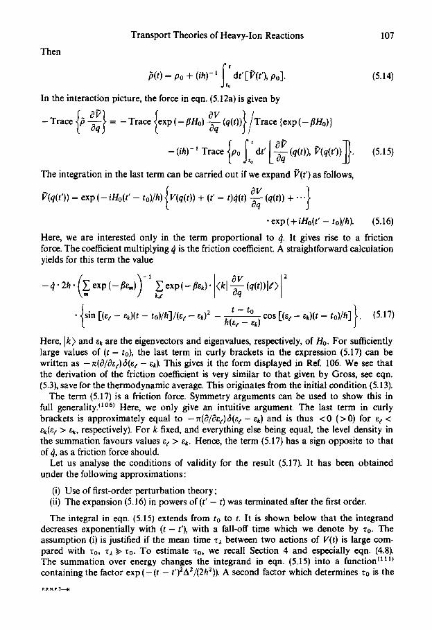
Transport Theories of Heavy-Ion Reactions 107
Then
~ t ~(t) = Po + (ih)-I dt' [ ~'(t'), Po]. (5.14) o
In the interaction picture, the force in eqn. (5.12a) is given by
- T r a c e {/5 ~---~} = - T r a c e { e x p ( - f l H o ) ~ q ( q ( t ) ) } / T r a c e { e x p ( - f l H o ) }
-(ih)-l Trace {po ltl dt' [-~q (q(t)), ~'(q(t'))]~. (5.15)
The integration in the last term can be carried out if we expand ~'(t') as follows,
~'(q(t')) = exp (-iHo(t' - to)/h) {V(q(t)) + (t' - t)(l(t) ~q (q(t)) + " .}
• exp(+iHo(t'- to)/h). (5.16)
Here, we are interested only in the term proportional to ~. It gives rise to a friction force. The coefficient multiplying t~ is the friction coefficient. A straightforward calculation yields for this term the value
- 0 " 2 h " exp ( - # ~ ) ~.,exp(-flek)" (kl --~ k,¢
• sin [(et - ek)(t -- to)/h]/(t: -- ek) 2 h(~: - ek) cos [(e: - ek)(t -- to)/h] . (5.17)
Here, Ik) and ek are the eigenvectors and eigenvalues, respectively, of Ho. For sufficiently large values of (t - to), the last term in curly brackets in the expression (5.17) can be written as -n(0/0et)6(ee - e~). This gives it the form displayed in Ref. 106. We see that the derivation of the friction coefficient is very similar to that given by Gross, see eqn. (5.3), save for the thermodynamic average. This originates from the initial condition (5.13).
The term (5.17) is a friction force. Symmetry arguments can be used to show this in full generality. ~°6) Here, we only give an intuitive argument. The last term in curly brackets is approximately equal to - g ( 0 / 0 e t ) 6 ( ~ t - ek) and is thus < 0 (>0) for e: < ek(er > ek, respectively). For k fixed, and everything else being equal, the level density in the summation favours values et > ek. Hence, the term (5.17) has a sign opposite to that of q, as a friction force should.
Let us analyse the conditions of validity for the result (5.17). It has been obtained under the following approximations:
(i) Use of first-order perturbation theory; (ii) The expansion (5.16) in powers of (t' - t) was terminated after the first order.
The integral in eqn. (5.15) extends from to to t. It is shown below that the integrand decreases exponentially with (t - t'), with a fall-off time which we denote by 3o. The assumption (i) is justified if the mean time ~ between two actions of V(t) is large com- pared with Zo, z~ "> To. To estimate To, we recall Section 4 and especially eqn. (4.8). The summation over energy changes the integrand in eqn. (5.15) into a function ~1~) containing the factor exp ( - ( t - t')2A2/(2h2)). A second factor which determines ro is the
P.P.N.P.3--H
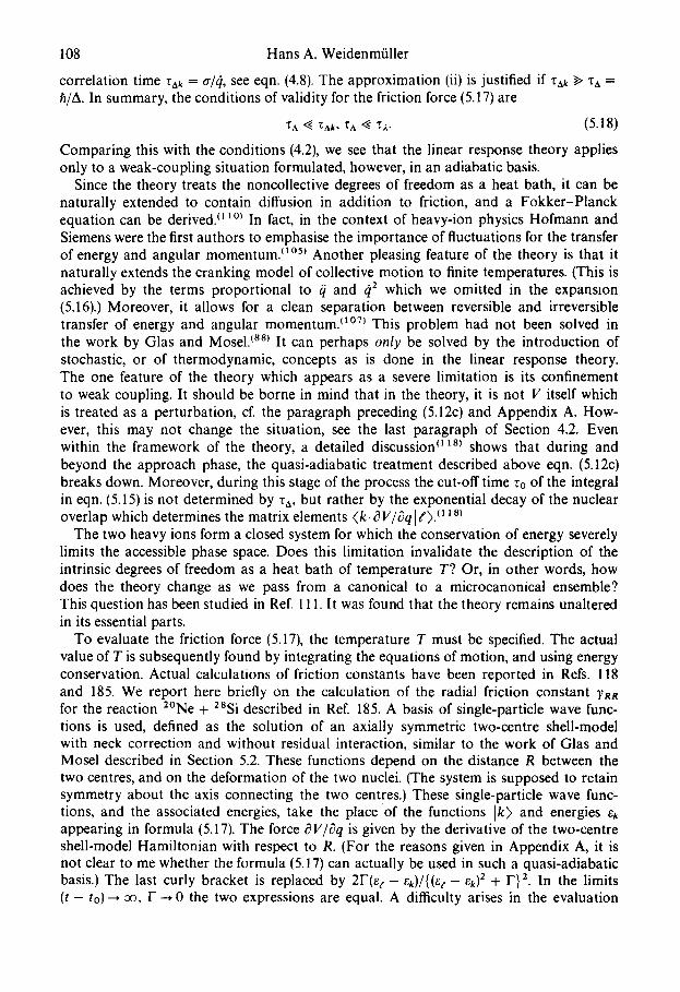
108 Hans A. Weidenmfiller
correlation time Z~k = a/~t, see eqn. (4.8). The approximation (ii) is justified if ZAR ~> ZA = h/A. In summary, the conditions of validity for the friction force (5.17) are
ZA <~ Z~k, ZA ~ ~ . (5.18)
Comparing this with the conditions (4.2), we see that the linear response theory applies only to a weak-coupling situation formulated, however, in an adiabatic basis.
Since the theory treats the noncollective degrees of freedom as a heat bath, it can be naturally extended to contain diffusion in addition to friction, and a Fokker-Planck equation can be derived. ~ ~o~ In fact, in the context of heavy-ion physics Hofmann and Siemens were the first authors to emphasise the importance of fluctuations for the transfer of energy and angular momentum. ~°5~ Another pleasing feature of the theory is that it naturally extends the cranking model of collective motion to finite temperatures. (This is achieved by the terms proportional to /j and ~2 which we omitted in the expansion (5.16).) Moreover, it allows for a clean separation between reversible and irreversible transfer of energy and angular momentum. ~°7) This problem had not been solved in the work by Glas and Mosel. ~sS) It can perhaps only be solved by the introduction of stochastic, or of thermodynamic, concepts as is done in the linear response theory. The one feature of the theory which appears as a severe limitation is its confinement to weak coupling. It should be borne in mind that in the theory, it is not V itself which is treated as a perturbation, cf. the paragraph preceding (5.12c) and Appendix A. How- ever, this may not change the situation, see the last paragraph of Section 4.2. Even within the framework of the theory, a detailed discussion ~l~s) shows that during and beyond the approach phase, the quasi-adiabatic treatment described above eqn. (5.12c) breaks down. Moreover, during this stage of the process the cut-off time t0 of the integral in eqn. (5.15) is not determined by zA, but rather by the exponential decay of the nuclear overlap which determines the matrix elements (k ] O V/Oq I ~) '~ ~ s~
The two heavy ions form a closed system for which the conservation of energy severely limits the accessible phase space. Does this limitation invalidate the description of the intrinsic degrees of freedom as a heat bath of temperature T? Or, in other words, how does the theory change as we pass from a canonical to a microcanonical ensemble? This question has been studied in Ref. 111. It was found that the theory remains unaltered in its essential parts.
To evaluate the friction force (5.17), the temperature T must be specified. The actual value of T is subsequently found by integrating the equations of motion, and using energy conservation. Actual calculations of friction constants have been reported in Refs. 118 and 185. We report here briefly on the calculation of the radial friction constant Yen for the reaction 2°Ne + 2sSi described in Ref. 185. A basis of single-particle wave func- tions is used, defined as the solution of an axially symmetric two-centre shell-model with neck correction and without residual interaction, similar to the work of Glas and Mosel described in Section 5.2. These functions depend on the distance R between the two centres, and on the deformation of the two nuclei. (The system is supposed to retain symmetry about the axis connecting the two centres.) These single-particle wave func- tions, and the associated energies, take the place of the functions I k) and energies ek appearing in formula (5.17). The force dV/Oq is given by the derivative of the two-centre shell-model Hamiltonian with respect to R. (For the reasons given in Appendix A, it is not clear to me whether the formula (5.17) can actually be used in such a quasi-adiabatic basis.) The last curly bracket is replaced by 2F(e t - ek)/{(er -- e,k) z + F} z. In the limits (t - to) ~ oo, F ~ 0 the two expressions are equal. A difficulty arises in the evaluation
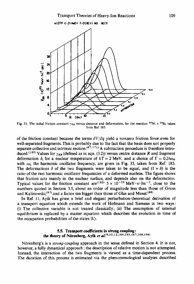
i¢1
"2- 8
Transport Theories of Heavy-Ion Reactions
MIOTH O.211"NOI T=2(fl[v,I NO
/ ! ,
NECK
/
/
/ / \ x \ 4 "
5 R (fro) tO t5
109
Fig. 33. The radial friction constant "tee versus distance and deformation, for the reaction 2°Ni + 28Si, taken from Ref. 185.
of the friction constant because the terms OV/Oq yield a nonzero friction force even for well-separated fragments. This is probably due to the fact that the basis does not properly separate collective and intrinsic motion. ~ST' ~Tz) A subtraction procedure is therefore intro- duced. (185) Values for ~R~ (defined as in eqn. (3.2)) versus centre distance R and fragment deformation 6, for a nuclear temperature of kT = 2 MeV, and a choice of F = 02hOJo with COo the harmonic oscillator frequency, are given in Fig. 33, taken from Ref. 185. The deformations 6 of the two fragments were taken to be equal, and (1 + 6) is the ratio of the two harmonic oscillator frequencies of a deformed nucleus. The figure shows that friction acts mainly in the nuclear surface, and depends also on the deformation. Typical values for the friction constant are (185) 5 x 10 -22 M e V . s . f m -2, close to the numbers quoted in Section 3.5, about an order of magnitude less than those of Gross and Kalinowski, (97) and a factor ten bigger than those of Glas and Mosel. (sS)
In Ref. 11, Ayik has given a brief and elegant perturbation-theoretical derivation of a transport equation which extends the work of Hofmann and Siemens in two ways: (i) The collective variable is not treated classically; (ii) The assumption of internal equilibrium is replaced by a master equation which describes the evolution in time of the occupation probabilities of the states Ik).
5.5. Transport coefficients in strong coupling: the theory of N6renberg, Ayik et aL {9'10'12'164'165'167"168'194)
N6renberg's is a strong-coupling approach in the sense defined in Section 4. It is not, however, a fully dynamical approach : the description of relative motion is not attempted. Instead, the interaction of the two fragments is viewed as a time-dependent process. The duration of this process is estimated via the phenomenological analyses described
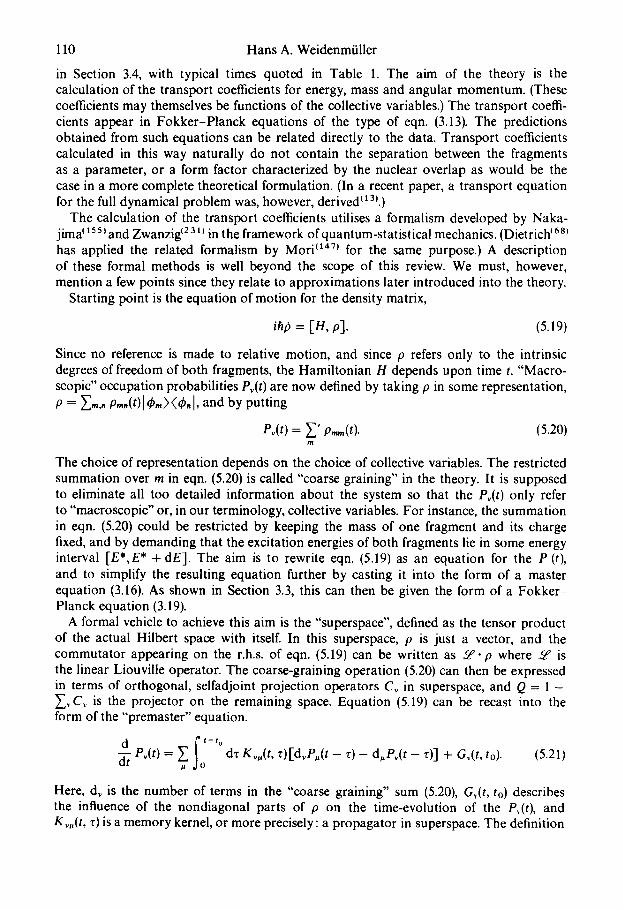
110 Hans A. Weidenmtiller
in Section 3.4, with typical times quoted in Table 1. The aim of the theory is the calculation of the transport coefficients for energy, mass and angular momentum. (These coefficients may themselves be functions of the collective variables.) The transport coeffi- cients appear in Fokker-Planck equations of the type of eqn. (3.13). The predictions obtained from such equations can be related directly to the data. Transport coefficients calculated in this way naturally do not contain the separation between the fragments as a parameter, or a form factor characterized by the nuclear overlap as would be the case in a more complete theoretical formulation. (In a recent paper, a transport equation for the full dynamical problem was, however, derived~a()
The calculation of the transport coefficients utilises a formalism developed by Naka- jima~a55~and Zwanzig t2al~ in the framework of quantum-statistical mechanics. (Dietrich 16a~ has applied the related formalism by Mori °47) for the same purpose.) A description of these formal methods is well beyond the scope of this review. We must, however, mention a few points since they relate to approximations later introduced into the theory.
Starting point is the equation of motion for the density matrix,
iht) = [H, p]. (5.19)
Since no reference is made to relative motion, and since p refers only to the intrinsic degrees of freedom of both fragments, the Hamiltonian H depends upon time t. "Macro- scopic" occupation probabilities P,( t ) are now defined by taking p in some representation, P = Z. , , . p,..(t)[ ~, . ) (4, .1 , and by putting
P~(t) = ~ ' p,,,,(t). (5.20) ?11
The choice of representation depends on the choice of collective variables. The restricted summation over m in eqn. (5.20) is called "coarse graining" in the theory. It is supposed to eliminate all too detailed information about the system so that the Pv(t) only refer to "macroscopic" or, in our terminology, collective variables. For instance, the summation in eqn. (5.20) could be restricted by keeping the mass of one fragment and its charge fixed, and by demanding that the excitation energies of both fragments lie in some energy interval [E*,E* + dE]. The aim is to rewrite eqn. (5.19) as an equation for the P (t), and to simplify the resulting equation further by casting it into the form of a master equation (3.16). As shown in Section 3.3, this can then be given the form of a Fokker- Planck equation (3.19).
A formal vehicle to achieve this aim is the "superspace", defined as the tensor product of the actual Hilbert space with itself. In this superspace, p is just a vector, and the commutator appearing on the r.h.s, of eqn. (5.19) can be written as ~ - p where £P is the linear Liouville operator. The coarse-graining operation (5.20) can then be expressed in terms of orthogonal, selfadjoint projection operators C~ in superspace, and Q = 1 - Y',~C,. is the projector on the remaining space. Equation (5.19) can be recast into the form of the "premaster" equation.
_d P~(t) d z Kv . ( t , r ) [ d v P . ( t - z) - d . P v ( t - z)] + G~(t, to). (5.21)
dt
Here, d~ is the number of terms in the "coarse graining" sum (5.20), G,.(t, to) describes the influence of the nondiagonal parts of p on the time-evolution of the P,.(t), and K ~.(t, z) is a memory kernel, or more precisely: a propagator in superspace. The definition
Transport Theories of Heavy-Ion Reactions 111
of K contains the factor ~65~ e x p [ - i Q j'~_, dt' ~(t ')] . The meaning of the symbol to is immaterial for what follows.
Although different in appearance, eqn. (5.21) is completely equivalent to the von Neumann equation (5.19). As soon as some approximations are introduced, however, eqn. (5.21) becomes the master equation of an irreversible process. Technically, one assumes that the matrix elements of Le are randomly (Gaussian) distributed. Then, the system quickly loses phase-memory. Moreover, all off-diagonal elements of 19 die off quickly, and Gv(t, to) vanishes after some equilibration time %q.. The memory kernel Kvu falls off during a very short time, called the "memory time", and it is assumed that during this time, Pv changes little. Then, Pv can be taken out from under the time integration, and the master equation (3.16) results.
This procedure does not constitute a strict derivation of the master equation. It can only suggest the conditions under which such an equation is valid. However, by applying it, expressions for the transition rates are obtained and from these, transport coefficients can be calculated.
It was just mentioned that in the derivation it is assumed that the Liouville operator introduced above has a random (Gaussian) probability distribution. Such an assump-
tion is similar to, but different from, the assumption introduced in eqn. (4.8). The differ- ence is that the Gaussian distribution is assumed for ~ , an operator in superspace, rather than for the matrix elements of V itself. With this assumption, one finds, slightly altering the notation of Ref. 165,
g, , ( t , r) = 2h- 2<1 vm.(t)]2>.,, exp { - r2/(2zg~)2}, (5.22)
where the bracket indicates an average over the states n, m lying in the coarse-graining cells v/~, respectively, and where
r.,o, = h <l v.,(t)12>, + ~ <1 v.,~12 >. (5.23)
Equations (5.22) and (5.23) bear a strong similarity to the strong-coupling equations (4.12a) and (4.12b), respectively. The difference is mainly the appearance of the pair of indices v, #, and of the two associated terms on the r.h.s, of eqn. (5.23). Disregarding this difference, and performing the summation over i , j in eqn. (5.23) with the help of eqn. (4.8), I find exactly the result (4.12b) save for a factor (8/n) ~/4 --- 1.26. This shows that Nrrenberg's "memory time" is the same physical quantity as the za introduced in Section 4. Numerically, r,,m is estimated as 2 × 10-22 s, in rough agreement with the relations (4.5). The energy loss per single action of V is estimated via the momentum transfer, the latter as h/R with R ~ 10 fm the distance between the two centres. In Section 4, we had also introduced the momentum transfer, and had estimated it to be hkv/5 = h/a with a = 3.5 fm. Nrrenberg's estimate is a factor 3 smaller. Therefore, his energy transfer per action of V is only about 2 MeV, and his r ~ = 6 × 10-23 s, also a factor 3 smaller than our value (4.4). I believe that this is an underestimate, and that the value (4.4) is more realistic. The quantity ra is estimated as h/A = zn~, so that the two times z a and zar introduced in Section 4 are always put equal in this theory.
Having arrived at a very short value for r,,,,., Nrrenberg et al. argue that during such times, P, changes very little and can be taken out from under the integral in eqn. (5.21). This step establishes the Markov approximation. It leads to an irreversible trans- port equation. It was shown below eqn. (3.21) that the Markov approximation is valid in the weak-couplin# limit. Now we face the situation that strong coupling leads to short
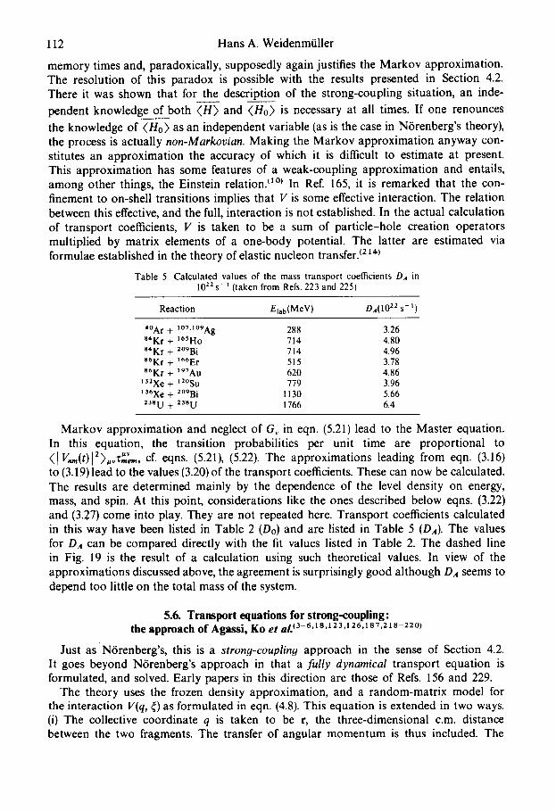
112 Hans A. Weidenmiiller
memory times and, paradoxically, supposedly again justifies the Markov approximation. The resolution of this paradox is possible with the results presented in Section 4.2. There it was shown that for the description of the strong-coupling situation, an inde-
pendent knowledge of both ( H ) and (Ho) is necessary at all times. If one renounces
the knowledge of (Ho) as an independent variable (as is the case in N6renberg's theory), the process is actually non-Markovian. Making the Markov approximation anyway con- stitutes an approximation the accuracy of which it is difficult to estimate at present. This approximation has some features of a weak-coupling approximation and entails, among other things, the Einstein relation] :°) In Ref. 165, it is remarked that the con- finement to on-shell transitions implies that V is some effective interaction. The relation between this effective, and the full, interaction is not established. In the actual calculation of transport coefficients, V is taken to be a sum of particle-hole creation operators multiplied by matrix elements of a one-body potential. The latter are estimated via formulae established in the theory of elastic nucleon transfer/2 x,~
Table 5. Calculated values of the mass transport coefficients DA in 1022s -. t Itaken from Refs. 223 and 225)
Reaction Elab(MeV ) DA(1022 s- t)
4°Ar + l°TA°9Ag 288 3.26 8"Kr + 165Ho 714 4.80 S4Kr + 2°9Bi 714 4.96 a6Kr + ~66Er 515 3.78 S6Kr + 197All 620 4.86
tS2Xe + a2°Su 779 3.96 136Xe + 2°9Bi 1130 5.66 23sU + 23sU 1766 6.4
Markov approximation and neglect of G~ in eqn. (5.21) lead to the Master equation. In this equation, the transition probabilities per unit time are proportional to (1 vm(t) 2- . ~ 2,,vt~,~, cf. eqns. (5.21), (5.22). The approximations leading from eqn. (3.16) to (3.19)lead to the values (3.20) of the transport coefficients. These can now be calculated. The results are determined mainly by the dependence of the level density on energy, mass, and spin. At this point, considerations like the ones described below eqns. (3.22) and (3.27) come into play. They are not repeated here. Transport coefficients calculated in this way have been listed in Table 2 (Do) and are listed in Table 5 (DA). The values for DA can be compared directly with the fit values listed in Table 2. The dashed line in Fig. 19 is the result of a calculation using such theoretical values. In view of the approximations discussed above, the agreement is surprisingly good although DA seems to depend too little on the total mass of the system.
5.6. Transport equations for strong-coupling: the approach of Agassi, Ko e t a l . ~3-6" 18.x 2 3, t 2 6, ~ a 7 ,2 t a - 2 2 o)
Just as N6renberg's, this is a strong-coupliny approach in the sense of Section 4.2. It goes beyond N6renberg's approach in that a fully dynamical transport equation is formulated, and solved. Early papers in this direction are those of Refs. 156 and 229.
The theory uses the frozen density approximation, and a random-matrix model for the interaction V(q, ~) as formulated in eqn. (4.8). This equation is extended in two ways. (i) The collective coordinate q is taken to be r, the three-dimensional c.m. distance between the two fragments. The transfer of angular momentum is thus included. The
Transport Theories of Heavy-Ion Reactions 113
random-matrix hypothesis is formulated for the reduced matrix elements of V. (ii) The exchange of mass and charge is taken into account. For this purpose, the definition of the states la>, Ib>... is generalized to include the label Z1, i.e. the atomic number of one of the two fragments. It is assumed that in this variable, the second moment of V also has a Gaussian form (an extra factor exp [ - ( Z l - Z2)2)/(262(Z~ + Z2)2)] appears on the r.h.s, of eqn. (4.8)), so that inelastic scattering (no change of Zt) is most probable. The dimensionless width 6 is a free parameter.
It was mentioned in Section 4.2 that this ansatz for the distribution of the matrix elements of V has been derived from the physical picture developed in Section 4.1, and from a random-matrix model for the states la>, [b>,...~ls) This derivation includes the angular momentum dependence of the reduced matrix elements, but is confined to inelastic scattering only. The parametrization of the Z~-dependence of the second moment just described is thus so far without microscopic justification.
The further development of the theory does not make use of the semi-classical approxi- mation for r, and thus proceeds in a different fashion from Section 4.2. The formal expression for the cross-section for inelastic scattering is used as a starting point. This cross-section depends in a highly nonlinear fashion on V. The avera#e cross-section is defined as a mean over a sufficiently wide energy interval. This mean value is calculated using the Gaussian distribution of the matrix elements of V. In the evaluation, the equality of energy average and ensemble average is used. ~s°'~st) Some essential steps in the calculation of the mean value c3) are given in Appendix B. Foremost among these is the identification of a small parameter y. The average of the cross-section is expanded in powers of y, and only terms of lowest non-vanishing (zeroth) order are kept. The parameter y is defined by y = m a x ( rAg / '~Po inca r~ , Z;./'CPoincare , "Ca/TPoincar~,) where the various r's were introduced in Section 4. The limit y--* 0 (ZPoincar~: ~ o0) corresponds to the thermodynamic limit. While the cross-sections themselves describe fully reversible pro- cesses, their mean values are quantities which display irreversible behaviour. It is thus through the statistical assumptions (4.8), and the calculation of averages, that irreversibility is introduced into the theory.
The resulting expression for the average cross-section still contains the values of the spins of the states of both fragments. A summation over the spins of the final and inter- mediate states can be performed: 3~ As a result, one finds a transport equation.
For simplicity of presentation, we display this transport equation only for the case where r is replaced by the one-dimensional variable q, and we omit the dependence of the state vectors la>, Ib> . . . . on the atomic number ZI. The Hamiltonian then has the form of eqn. (4.7), the statistical assumptions are those of eqn. (4.8). Let St÷~(q, ~) be the scattering eigenfunction of the full Hamiltonian (4.7) subject to the boundary con- dition that there be an incoming wave only in channel a. The mean density matrix of the system is defined by
fib° = (b] ~k~÷'(q, ~)) (~O~+)(q ', ~')]b>. (3.24)
It is obvious that the asymptotic form of Pbo(q, q') for I ql--' ~ , I q'l--' ~ yields the average cross-section for the transition a--* b. A comparison with eqn. (4.13) shows that, in the time-independent theory, fiba(q, q') is the analogue of the density matrix fib,(t, t').
It is useful to introduce the Wigner transform Fbo(q, p) of Pbo(q, q'). It is defined by
Fb~(q, p) = (2n)- ~ f d~ exp ( - ip¢)fibo(q + ½¢, q - (5.25) d
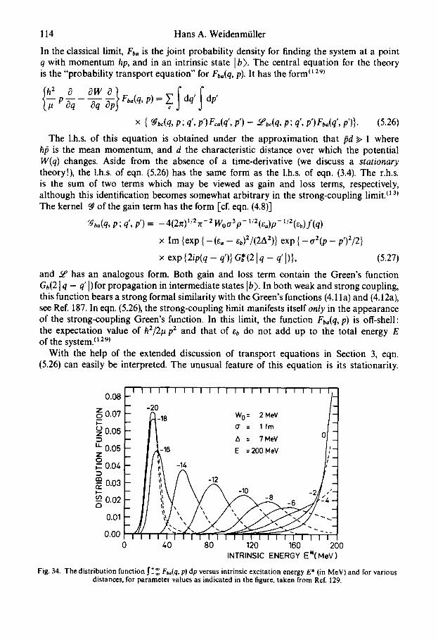
114 Hans A. Weidenmiiller
In the classical limit, Fb, is the joint probability density for finding the system at a point q with momentum hp, and in an intrinsic state I b>. The central equation for the theory is the "probability transport equation" for Fbo(q, p). It has the form (~29)
0 { ,oo oo x { qJ~c(q,p;q',p')Fco(q',p')- -~bc(q,p;q',p')Fb°(q',p')}. (5.26)
The 1.h.s. of this equation is obtained under the approximation that ~0d ,> 1 where h~0 is the mean momentum, and d the characteristic distance over which the potential W(q) changes. Aside from the absence of a time-derivative (we discuss a stationary theory!), the l.h.s, of eqn. (5.26) has the same form as the l.h.s, of eqn. (3.4). The r.h.s. is the sum of two terms which may be viewed as gain and loss terms, respectively, although this identification becomes somewhat arbitrary in the strong-coupling limit. (13) The kernel ~ of the gain term has the form [c£ eqn. (4.8)]
(¢ba(q, P; q', P') = -4(2rt)il21z -2 WotTaP - l i2 (ga)p - l /2 (gb) f (q )
x lm {exp { - (Co - e/,)2/(2A2)} exp { - o ' 2 ( p - - / ) 2 / 2 }
x exp {2ip(q - q')} G~'(21 q - q' I)}, (5.27)
and ~ has an analogous form. Both gain and loss term contain the Green's function Gb(21q -- q'D for propagation in intermediate states Ib ). In both weak and strong coupling, this function bears a strong formal similarity with the Green's functions (4.1 l a) and (4.12a), see Ref. 187. In eqn. (5.26), the strong-coupling limit manifests itself only in the appearance of the strong-coupling Green's function. In this limit, the function Fbo(q, p) is off-shell: the expectation value of h2/21.t p2 and that of eb do not add up to the total energy E of the system. (~ 29)
With the help of the extended discussion of transport equations in Section 3, eqn. (5.26) can easily be interpreted. The unusual feature of this equation is its stationarity.
0 . 0 8 on / ~oo7~ ~_,~ ~o~ ~.:v /~ ~°°°1= il ~: ;=v °/:1 ~.oo, 1= IA~, ~ ,=..v I;-t ~°°'E I1~1 ;t i"~ ~°°~V II i t / \ * _,o _ _J,,~ ~o.o~ II !7,, X ~ : ' : 1
°.°'i:_7J - . - - -1 0 " 0 0 1 I I I I I I I I 1 I I I I I I I I I I - 1 I I I I
0 40 80 120 160 200 INTRINSIC ENERGY E~(MeV)
Fig. 34. The distribution function S-*~ F~(q, p) dp versus intrinsic excitation energy E* (in MeV) and for various distances, for parameter values as indicated in the figure, taken from Ref. 129.
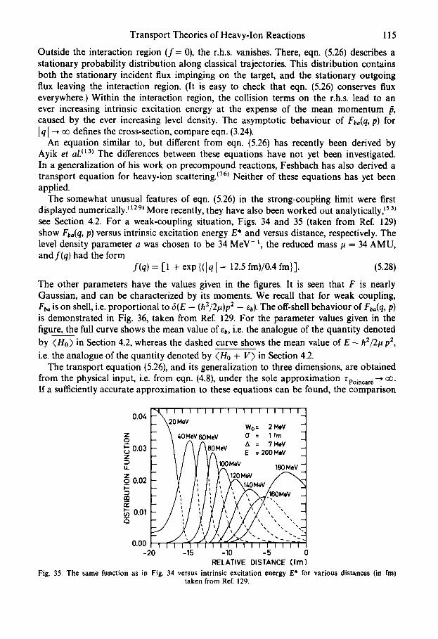
Transport Theories of Heavy-Ion Reactions 115
Outside the interaction region ( f = 0), the r.h.s, vanishes. There, eqn. (5.26) describes a stationary probability distribution along classical trajectories. This distribution contains both the stationary incident flux impinging on the target, and the stationary outgoing flux leaving the interaction region. (It is easy to check that ¢qn. (5.26) conserves flux everywhere.) Within the interaction region, the collision terms on the r.h.s, lead to an ever increasing intrinsic excitation energy at the expense of the mean momentum /~, caused by the ever increasing level density. The asymptotic behaviour of Fb°(q, p) for [ q [ ~ ~ defines the cross-section, compare ¢qn. (3.24).
An equation similar to, but different from ¢qn. (5.26) has recently been derived by Ayik et al. It3~ The differences between these equations have not yet been investigated. In a generalization of his work on precompound reactions, Feshbach has also derived a transport equation for heavy-ion scattering, c~6~ Neither of these equations has yet been applied.
The somewhat unusual features of eqn. (5.26) in the strong-coupling limit were first displayed numerically, t 1291 More recently, they have also been worked out analytically, Is 3) see Section 4.2. For a weak-coupling situation, Figs. 34 and 35 (taken from Ref. 129) show Fb=(q, p) versus intrinsic excitation energy E* and versus distance, respectively. The level density parameter a was chosen to be 34 MeV- z, the reduced mass/~ = 34 AMU, andf(q) had the form
f ( q ) = [1 + ¢ x p { ( [ q l - 12.5 fm)/0.4 fm}]. (5.28)
The other parameters have the values given in the figures. It is seen that F is nearly Gaussian, and can be characterized by its moments. We recall that for weak coupling, Fb= is on shell, i.e. proportional to 6(E - (h2/21~)p 2 - eb). The off-shell behaviour of Fb°(q, p) is demonstrated in Fig. 36, taken from Ref. 129. For the parameter values given in the figure, the full curve shows the mean value of ~b, i.e. the analogue of the quantity denoted by (Ho> in Section 4.2, whereas the dashed curve shows the mean value of E - h 2 / 2 ~ p2 i.e. the analogue of the quantity denoted by <H0 + V> in Section 4.2.
The transport equation (5.26), and its generalization to three dimensions, are obtained from the physical input, i.e. from eqn. (4.8), under the sole approximation ZPoincar~ ~ ~ . If a sufficiently accurate approximation to these equations can be found, the comparison
, , , , , ,_
~ "~OMeV Wo = 2Mev _
Z [_. \ 40MeV60MeV O = 1 fm - 0 . 0 3 A = .1/MeV -
eV E = 200 MeV - z
= I- I/ V Y '''v ,8o,,,,v- " I:: V I, P, I o.o21_ /', /',/', /, ° -
m_
o . o o ~ ~ t t t T t ~ t f t ~ t ~ t t ~ i t -20 -15 -10 -5 0
RELATIVE DISTANCE (fm) Fig. 35. The same function as in Fig. 34 versus intrinsic excitation energy E* for various distances (in fro)
taken from Rcf. 129.
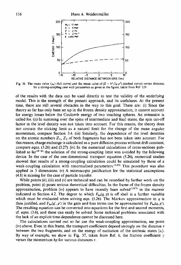
116
200
150 >=
loo
,,=, 5O
Hans A. Weidenmfiller
i
Wo= 12MeV A = 5 M e V (2" : 2 fm 11 = 2 fm -1 E =200 MeV
i i i
0 1 1 L I 0 -15 -10 - 5 0 5 10
200
150
100
50
RELATIVE DISTANCE BETWEEN IONS ( fm)
Fig. 36. The mean value (eb) (full curve) and the mean value of (E - h2/2# p2) (dashed curve) versus distance, for a strong-coupling case with parameters as given in the figure, taken from Ref. 129.
of the results with the data can be used directly to test the validity of the underlying model. This is the strength of the present approach, and its usefulness. At the present time, there are still several obstacles in the way to this goal. These are: (i) Since the theory so far has only been set up in the frozen density approximation, it cannot account for energy losses below the Coulomb energy of two touching spheres. An extension is called for. (ii) In summing over the spins of intermediate and final states, the spin cut-off factor in the level density was not taken into account. For this reason, the theory does not contain the sticking limit as a natural limit for the change of the mean angular momentum, compare Section 3.4. (iii) Similarly, the dependence of the level densities on the atomic numbers Z, , Z2 of both fragments has not been taken into account. For this reason, charge exchange is calculated as a pure diffusion process without drift constant, compare eqns. (3.26) and (3.27). (iv) In the numerical calculations of cross-sections pub- lished so far (a-6) the solution of the strong-coupling limit was avoided by the following device. In the case of the one-dimensional transport equation (5.26), numerical studies showed that results of a strong-coupling calculation could be simulated by those of a weak-coupling calculation with renormalised parameters. (129) This procedure was also applied in 3 dimensions. (v) A microscopic justification for the statistical assumptions (4.8) is missing for the case of particle transfer.
While points (ii), (iii) and (v) are technical and can be remedied by further work on the problem, point (i) poses serious theoretical difficulties. In the frame of the frozen density approximation, problem (iv) appears to have recently been solved (t87) in the manner indicated in Section 4.2. The degree to which Fba(q, p) is off shell is a further variable which must be evaluated when solving eqn. (5.26). The Markov approximation in q is then justified, and Fb,,(q', p') in the gain and loss terms can be approximated by Fb,,(q, p'). The resulting equation can be converted into equations for the first and second moments, cf. eqns. (3.6), and these can easily be solved. Some technical problems associated with the lack of an explicit time-dependence cannot be discussed here.
The calculations carried out so far use the weak-coupling approximation, see point (iv) above. Even in this frame, the transport coefficients depend strongly on the distance r between the two fragments, and on the energy of excitation of the intrinsic states la>. By way of example, we show in Fig. 37, taken from Ref. 6, the friction coefficient 7 versus the momentum hp for various distances r.
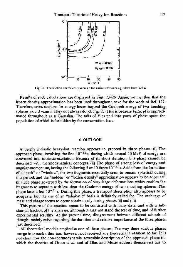
Transport Theories of Heavy-Ion Reactions
' I ' 1 1 1 ' 1 '
; ? " + 1 Fn ~ F. ~ r 8,
~ 10-2
+
117
I~Kr . 201pb
ELAB : 715HeV
10 -'~ 1 1 I I 10 20 30 40 50
p (fm -!)
Fig. 37. The friction coefficient 7 versus p for various distances q, taken from Ref. 6.
Results of such calculations are displayed in Figs. 23-26. Again, we mention that the frozen density approximation has been used throughout, save for the work of Ref. 127. Therefore, cross-sections for energy losses beyond the Coulomb energy of two touching spheres would vanish. They not always do, cf. Fig. 23. This is because Fb°(q, p) is approxi- mated throughout as a Gaussian. The tails of F extend into parts of phase space the population of which is forbidden by the conservation laws.
6. OUTLOOK
A deeply inelastic heavy-ion reaction appears to proceed in three phases. (i) The approach phase, involving the first 10 -22 s, during which several 10 MeV of energy are converted into intrinsic excitation. Because of its short duration, this phase cannot be described with thermodynamical concepts. (ii) The phase of strong loss of energy and angular momentum, lasting the following 5 or 10 times 10-22 s. Aside from the formation of a "neck" or "window", the two fragments essentially seem to remain spherical during this period, and the "sudden" or "frozen density" approximation appears to be adequate. (iii) The phase governed by the formation of very large deformations which enables the fragments to separate with less than the Coulomb energy of two touching spheres. This phase lasts a few 10 -21 s. During this phase, a transport description also appears to be adequate, but the use of an "adiabatic" basis is definitely called for. The exchange of mass and charge seems to occur continuously during phases (ii) and (iii).
This picture of the reaction seems to be consistent with many data, and with a sub- stantial fraction of the analyses, although it may not stand the test of time, and of further experimental scrutiny. At the present time, disagreement between different schools of thought mainly exists regarding the duration and relative importance of the three phases just described.
All theoretical models emphasise one of these phases. The way these various phases merge into each other has, however, not received any theoretical treatment so far. It is not clear how the non-thermodynamic, reversible description of the approach phase (to which the theories of Gross et al. and of Glas and Mosel address themselves) has to
118 Hans A. Weidenmiiller
be joined with the (irreversible) transport theories of later phases. It is equally unclear how the transition between phases (ii) and (iii) should be described. In a fully dynamical calculation, the choice of basis is immaterial and a matter of convenience only. In a transport description, however, this is not so. What is counted as a reversible loss of energy in one basis, is partly counted as an irreversible loss in another, and vice versa. The transition between the phases characterised by different bases is therefore a chal- lenging problem.
Transport theoretical approaches exist to deal with phases (ii) and (iii) individually. The theory of Hofmann and Siemens is flexible, and can be used in either context, although the Hofmann-Siemens theory is formulated primarily for an adiabatic basis. The theories of Swiatecki et al. ("window" formula), of N6renberg et al., and of Agassi et al., specifically use the sudden approximation, while the "wall" formula of Sawicki et al. may be viewed as being appropriate for the adiabatic basis.
Aside from the more technical problems, and problems of detail, besetting each of these theories, the foremost problem in any one of them is the identification and choice of the proper collective variables. For this purpose, it would be highly desirable to establish a theoretical link between these theories, and TDHF. Such a link does not exist.
Within their realm of applicability, the models of Broglia et al., of Swiatecki et al. ("window" formula), of N/Srenberg et al. and of Agassi et al. have yielded satisfactory agreement with the data. Although these models do start from the same basic picture, they differ sufficiently in detail to make this agreement bothersome. Are the existing data insensitive to such details of the theoretical formulation? In particular, is it possible to distinguish between the applicability of weak coupling versus that of strong coupling? These questions require a more detailed analysis. The agreement with the data should be subject to close scrutiny, as should be the inherent consistency of each model.
In my opinion, the theory is least well developed in two aspects. (i) No microscopic calculation of inertia, potential and transport coefficients exists as yet for phase (iii), which bears such a strong similarity to the final stages of fission. (ii) The transfer of mass and charge is little understood. Is this transfer a random walk problem, as assumed in some approaches, or is the collective motion of the mass variable overdamped? A unified description of deeply inelastic collisions, fusion, and fission, would be a long- term goal, only to be reached via a careful analysis of the relevant collective variables and of the associated time-scales.
Further open problems emerge upon a close look at the data. Some of these were mentioned at the end of Section 3. Others can be seen by looking at the qualitatively different results found at higher bombarding energies where the deeply inelastic collisions seem to disappear. ~199) The transition point is perhaps reached when the relative velocity between two heavy ions becomes comparable with the Fermi velocity of a nucleon. Do equilibration phenomena lack the time to occur at these and higher energies? Or does nuclear matter become brittle? Much about the limitation of transport theories, among other things, will be learned from the analysis of data in the domain 10-100 MeV/nucleon, and from the ensuing development of theoretical models.
Deeply inelastic heavy-ion collisions are exciting processes. They have baffled us by their very existence, they have offered many surprising features (and continue to do so), and the extension of concepts of statistical mechanics, and their application to these processes is an exciting enterprise. I am confident that the investigation of these reactions, and of heavy-ion collisions at somewhat higher energy, will continue to offer new dis- coveries, and to pose interesting problems, for a long while.
Transport Theories of Heavy-Ion Reactions 119
REFERENCES
I. ABUL-MAGD, A. Y., SIMBEL, M. H. and WInDENMf3LLER, H. A., Z. Phy. A285, 41 (1978). 2. AGASSX, D., WEIDENMOLLOt, H. A. and MANTZOURANIS, G., Phys. Lett. C22, 145 0975). 3. AGASSI, D., KO, C. M. and WEIDENMULLER, H. A., Ann. Phys. (N. Y.) 107, 140 (1977). 4. AGASSl, D., KO, C. M. and WEIDENMfJLLER, H. A., Ann. Phys. (N.Y.) i17, 407 (1979). 5. AGASSI, D., WEIDENMULLER, H. A. and Ko, C. M., Phys. Lett. 7313, 284 (1978). 6. AGASSI, D., KO, C. M., and WEIDENMfJLLER, H. A., Phys. Rev. C18, 223 (1978). 7. AGASSI, D., Preprint Rochester 1978. 8. AV1SHAI, Y., Z. Phys. A282, 347 (1977). 9. AYIg, S., SCHORMANN, B. and N6RENBERO, W., Z. Phys. A277, 299 (1976).
10. AYIK, S., SCHURMANN, B. and NORENBERG, W., Z. Phys. A279, 145 (1976). 11. AYIK, S., Phys. Lett. 63B, 22 (1976). 12. AYIK, S., WOLSCHIN, G. and N6RENaERG, W., Z. Phys. A286, 271 (1978). 13. AYIK, S. and N6RENBERG, W., Z. Phys. A2~, 401 (1978). 14. BASILF., R., GALIN, J., GUERREAU, D., L~ORT, M. and TARRAGO, X., J. Phys. (Paris) 33, 9 (1972). 15. BASS, R., Phys. Lett. 47B, 139 (1973). 16. BASS, R., Nucl. Phys. A231, 45 (1974). 17. BARANGER, M. arid VENERONI, M., Ann. Phys. 114, 123 0978). 18. BARRETT, B. R., SHLOMO, S. and WE1DENMIJLLEIR, H. A., Phys. Rev. C!7, 544 (1978). 19. BECglS~., R., Theorie der W¢irme, Springer Verlag, Heidelberg, 1964. 20. BECK, R. and GROSS, D. H. E., Phys. Lett. 47B, 143 (1973). 21. BeNEg, M. and LOMBARD, R. J., Ann. Phys. (N. Y.) 86, 262 (1974). 22. BECK, F., Phys. Lett. 62B, 385 (1976). 23. BERLANGER, M., GRANGE, P., HOFMANN, H., NGO, CH. and RICHERT, J., Preprint 1977 IPNO-RC-77-12
(unpublished). 24. BERTSCH, G., Les Houches Lectures 1977. 25. BERTSCH, G. and SCHAEFFER, S., Nucl. Phys. A277, 509 (1977). 26. BECK, F., BLOCKI, J., DWORZECKA, M. and WOLSCmN, G., Phys. Lett. 76B, 35 (1978). 27. BECK, F., DWORZECKA, M. and FELDMAIER, H., Z. Phys. A289, 113 (1978). 28. BERLANGER, M., NGO, CH., GRANGE, P., RICHERT, J. and HOFMANN, H., Z. Phys. A284, 61 (1978). 29. BERLANGER, M., GRANGE, P., HOFMANN, H., NGO, CH. and RICHERT, J., Z. Phys. A286, 207 (1978). 30. BILLEREY, R., CERRUTI, C., CHEVARIER, A. and DEMEYER, A., Z. Phys. A ~ , 399 (1978). 31: BIRKELUND, J. R., HUIZENGA, J. R., DE, J. N. and SPERBER, D., Preprint 1978. 32. BLATr, J. M. and WEISSKOPF, V. F., Theoretical Nuclear Physics, John Wiley, New York (1952). 33. BLOCH, C., Scientific works, Volume 2, editors BALIAN, R., DE DOmNICIS, C., G1LLEr, V., MESSIAH, A.,
North-Holland Publ. Co., Amsterdam (1975). 34. BLOCKI, H., ]~)NEH, Y., NIX, J. R., RANDRUP, J., ROBEL, M., SIERK, A. J. and SW1ATP.CKI, W. J., Ann.
Phys. (N. Y.) 113, 330 (1978). 35. BLOCKI, J., RANDRUP, J., SWlATECKI, W. J. and TSANG, C. F., Ann. Phys. (N. Y.) 105, 427 (1977). 36. BONEH, Y. and FRAENKEL, Z., Phys. Rev. C10, 893 (1974). 37. BONEH, Y., FRAENKEL, Z. and PALTIEL, Z., Physics and Chemistry of Fission, Rochester 1973, Vol. I, p. 515,
(IAEA, Vienna, 1974). 38. BONDORF, J. P., SOBEL, M. I. and SPERBER, D., Phys. Lett. 15C, 83 (1974). 39. BONDORF, J. P., Proc. Int. Conf. on Reactions between Complex Nuclei, Nashville 1974, Voi. 2, p. 383,
North-Holland Publ. Co., Amsterdam (1974). 40. BONDORF, J. P., HUIZENGA, J. R., SOBEL, M. I. and SPERn~, D., Phys. Rev. CII, 1265 (1975). 41. BONEH, Y., BLOCKI, J. P. and MYERS, W. D., Phys. Lett. 63B, 265 (1976). 42. BONDORF, J. P., LIOU, M. K., SOBEL, M. I. and SPERSER, D., Nuovo Cimento, Seric II, Vol. 42A, 1 (1977). 43. BRUECKNER, K. A., BUCHLER, J. R., JORNA, S. and LOMBARD, R. J., Phys. Rev. 171, 1188 (1968). 44. BRUECKNER, K. A., LIN, W. F. and LOMBARD, R. J., Phys. Rev. 181, 1543 (1969). 45. BRINK, D. M. and ROWLEV, N., Nucl. Phys. A219, 79 (1974). 46. BRINK, D. M. and STANCU, FI., Nucl. Phys. A243, 175 (1975). 47. BROGLIA, R. A., DASSO, C. H. and WINTHER, Aa., Phys. Lett. 61B, 113 (1976). 48. BROGLIA. R. A., DASSO, C. H., POLLAROLO, G. and WlNTHER, Aa., IPCR Symposium on Macroscopic
Features of Heavy-lon Collisions and Pre-equilibrium Processes, Hakone 1977, IPCR Cyclotron Progress Report Supplement 6, p. 251 (1977).
49. BROGLIA, R. A., C1VITARESE, O., DASSO, C. H. and WINTHER, Aa., Phys. Lett. 73B, 405 (1978). 50. BROSA, U. and KRAPPE, H. J., Z. Phys. A284, 65 (1978). 51. BROGL1A, R. A., DASSO, C. H., POLLAROLO, G. and WINTHER, Aa., Phys. Rev. Left. 41, 25 (1978). 52. BROGLIA, R. A., Invited Talk at the Int. Conf. on Dynamical Properties of Heavy-Ion Reactions, Johannes-
burg, South Africa, August 1978 (to be published). 53. BRINK, D. M., NEro, J. and WEIDENMULLER, H. A., Phys. l.ett. 80B, 170 (1979).
120 Hans A. Weidenmiiller
.54. BRODY, T. A., FLORES, J., MELLO, P. A., FRENCH, J. B. and WONG, S. S. M., Notas de Fisica, Vol. !, No. 3 (1978).
55. CHANDRASEKHAR, S., Rev. Mod. Phys. 15, 1 (1943). 56. DAVIES, R. H., Phys. Rev. C9, 2411 (1974). 57. DAVIES, K. T. R., SIERK, A. J. and NIX, R., Phys. Rev. C13, 2385 (1976). 58. DAVIES, K. T. R. and Nix, J. R., Phys. Rev. C14, 1977 (1976). 59. DAVIES, K. T. R., MARUHN-REZWANI, V., KOONIN, S. E. and NEGELE, J. W.. Phys. Rev. Lett. 41 632 (1978). 60. DASSO, C. H., DOSSING, T. and PAULI, H. C., Z. Phys. 289, 395 (1979). 61. DEUBLER, H. H. and DIETRICH, K., Phys. Lett. 56B, 241 (1975). 62. DE, J. N., GROSS, D. H. E. and KALINOWSKI, H., Z. Phys. A277, 385 (1976). 63. DE, J. N., Phys. Lett. 66B, 315 (1977). 64. DEUBLER, H. H. and DIETRICH, K., Nucl. Phys. A277, 493 (1977). 65. DE, J. N., GARPMAN, S. I. A., SHERMAN, A., SPERBER, D. and TAM, K., Phys. Lett. 7813, 13 (1978). 66. DE, J. N., GARPMAN, S. I. A., SPERBER, D. and TAM, K., Preprint Rensselaer 1978. 67. DE, J. N. and SPERBER, D., Phys. Lett. 72B, 293 (1978). 68. DIETRICH, K., Nucleonika 21, 89 (1976). 69. DIETRICH, K. and LECLERQ.-WILLAIN, CH., Ann. Phys. (N. Y.) 109, 41 (1977). 70. DIETRICH, K.. in: Dissipative Phenomena in Deep Inelastic Reactions, Preprint HMI-B 272 Berlin 1978
(unpublished). 71. DOVER, C. B. and VARY, J. P., Lecture Notes in Physics, Vol. 33, p. 1, Springer-Verlag, Berlin (1975). 72. EINSTEIN, A., Ann. Phys. 17, 549 (1905), ibid. 19, 371 (1906). 73. ESSEt., H., H^R~L, K., HENNING, W., KIENLE, P., K6RNER, H. J., REHM, K. E., SPERR, WAGNER, W., and
SPIELER, W., Z. Phys. A289, 265 (1979). 74. EYAL, Y., GAVRON, A., TSERRUYA, I., FRAENKEL, Z., EISEN, Y., WALD, S., BASS, R., GOULD, G. R.,
KREYLING, G., RENFORDT, R., STELZER, K., ZITZMANN, R., GOBB1, A., LYNEN, O., STELZER, H., RODE, I. and BOCK, R., Phys. Rev. Lett. 41,625 (1978).
75. FESHBACH, H., KERMAN, A. K. and LEMMER, R. H., Ann. Phys. (N. Y.) 41,230(1967). 76. FESHBACH, H., Notas di Fiscia, Vol. 1, No. 9, p. 111 (1978). 77. FLOCARD, H., Nucleonika, to be published. 78. FRASCARIA, N., STEPHAN, C., COLOMBANI, P., GARRON, J. P., JACMART, J. C., RIOU, M. and TASSAN-GOT, L.,
Phys. Rev. Lett. 39, 918 (1977). 79. FRASCARIA, N., COLOMBANI, P., GAMP, A., GARRON, J. P., JACMART, J. C., RIOU, M., ROYNETTE, J. C.,
STEPHAN, C., TASSAN-GOT, L., AMEHAUME, A., BIZARD, G., DUCHON, J., LAVILLE, J. L. and LOUVEL, M., in: Proceedings, Workshop on High-Resolution Heavy-Ion Physics at 20-100 MeV/A, Saclay, May 1978, p. 72.
80. FRENCH, J. B., MELLO, P. A. and PANnEr, A., Ann. Phys. (N.Y.} 113, 277 (1978). 81. GARG, J. B., ed. Statistical Properties of Nuclei, Plenum Press, New York (1972). 82. GALIN, J., GUERREAU, D., LEFORT, M. and TARRAGO, X., Phys. Rev. C9, 1018 (1974). 83. GALIN, J., GATrY, B., GUERREAU, D., LEFORT, i . , TARRAGO, X., BABINET, R., CAUVIN, B., GIRARD, J.
and NIFENECKER, H., Z. Phys. A278, 347 (1976). 84. GAMP, A., JACMART, J. C., POFFE, N., DOUBRE, H., ROYNETTE, J. C. and WILCZYNSKI, J., Phys. Lett. 74B,
215 (1978). 85. GELBKE, C. K., BINI, M., OLMER, C., HENDRIE, D. H., LAVILLE, J. L., MAHONEY, J., MERMAZ, M. C.,
SCOTT, D. K. and WIEMAN, H. H., Phys. Lett. 71B, 83 (1977). 86. GLAS, D. and MOSEL, U., Phys. Lett. 49B, 301 (1974). 87. GLAS, D., Z. Phys. A277, 195 (1976). 88. GLAS, D. and MOSEL, U., Nucl. Phys. A264, 268 (1976). 89. GOULD, C. R., BASS, R., CZARNECKI, J. V., HARTMANN, V., STELZER, K., ZITZMANN, R., EYAL, Y. Z. Phys.
A284, 353 (1978). 90. GROGS, D. H. E., KALINOWSKI, H., and BECK, R., Contribution 5.65, Proc. Int. Conf. Nucl. Phys., Munich
1973, J. DE BOER and H. J. MANG, ¢ds., p. 383, North-Holland Publ. Co., Amsterdam (1973). 91. GROSS, O. H. E. and KALINOWSKI, H., Phys. Lett. 48B, 302 (1974). 92. GROSS, D. H. E., KALINOWSKI, H. and DE, J. N., Lecture Notes in Physics, Vol. 33, p. 194, Springer Verlag,
Berlin (1975). 93. GROSS, D. H. E., Nucl. Phys. A240, 472 (1975). 94. GROSS, D. H. E. and KALINOWSKI, H., Invited Talk given at 4 ° session d'dtudes biennale de physique
nucldaire, La Toussiere, 1977 (unpublished). 95. GROSS, D. H. E., Phys. Lett. 68B, 412 (1977). 96. GRIFFIN, J. J., Proc. Third Int. Conf. Clustering Aspects of Nuclei, Winnipeq, June 1978, A.I.P., New York
1978 (in press). 97. GROSS, D. H. E. and KALINOWSKI, H., Phys. Lett. C45, 177 (1978). 98. HAGEMANN, G. B., BRODA, R., HERSKIND, B., ISHII-IARA, M., OGAZA, S., RYDE, H., Nucl. Phys. A245,
166 (I 975).
Transport Theories of Heavy-Ion Reactions 121
99. HARRIS, J. W., CORMIER, T. M., GEESAMAN, D. F., LEE, L. L., JR., MCGRAT~ R. L. and WURM, J. P., Phys. Rev. Left. 38, 1460 (1977).
100. HARA, K., in: Jahresbericht 1977, Beschleunioerlaboratorium der Universitfit und der Technischen Universitfit Mfmchen, p. 90 (unpublished).
101. HEUSCH, B., VOLANT, C., FREI~SLEBEN, H., CHESTNUT, R. P. HILDENnRAND, K. D., POHLHOFER, F., SCHNSDER, W. F. W., KOHLMEVER, B. and PFEFFER, W., Z. Phys. A288, 391 (1978).
102. HILSCHER, D., BIRKELUND, J. R., HOOVER, A. D., SCHR6D~, W. U., WILCXF~ W. W., HUIZENGA, J. R., MIGNEREV, A., WOLF, K. L., BREUER, H. and VIOLA, V. E., Phys. Rev. C20, 576 (1979).
103. HOFMANN, H. and SIEMENS, P. J., Vlllth European Conference on the Physics and Chemistry of Complex Nuclear Reactions, H66r, Sweden, September 1975 (unpublished).
104. HOFMANN, H., Xlll th International Winter Meeting on Nuclear Physics, Bormio, Italy, 1975 (unpublished) 105. HOFMANN, H. and SIEMENS, P. J., Phys. Lett. 58B, 417 (1975). 106. HOFMANN, H. and SIEMENS, P. J., Nucl. Phys. A257, 165 (1976). 107. HOFMANN, H. Phys. Lett. 61B, 423 (1976). 108. HOFMANN, H. and NGO, CH., Phys. tett. 65B, 97 (1976). 109. HOLZWARTH, G., Phys. Lett. 66B, 29 (1976). 110. HOFMANN, H. and SIEMENS, P. J., Nucl. Phys. A275, 464 (1977). 111. HOFMANN, H., Int. Syrup. Nuclear Coll. and their Microscopic Interpretation, Bled, Yugoslavia (1977):
Fisika 9, Suppl. 4 (1977). 112. HOF~ANN, H. and NGO, CH., Proc. Top. Conf. Heavy-lon Collisions, Fall Creek Falls State Park, Tennessee,
June 1977, Oak Ridge Conference Report CONF-770602, p. 259 (1977). 113. Ho, H., ALBRECHT, R., DONNWESER, W., GRAW, G., STEADMAN, S. G., WURM, J. P., DISDIER, D.,
RAUCH, V., SCHEmL1NG, F., Z. Phys. A283, 235 (1977). 114. HOLZWARTH, G. and ECKART. G.. Z. Phys. A284, 291 (1978). 115. HOLZWARTH, G. and ECKART, G., Nucl. Phys. A325, 1 (1979}. 116. HUIZENGA, J. R., BIRKELUND, J. R., SCHR6DF.R, W. U., WOLF, K. L. and VIOLA, V. E., JR., Phys. Rev.
Lett. 37, 885 (1976). 117. JEUKENNE, J. P., LFAEUNE, A. and MAHAUX, C., Phys. Lett. 25C, 83 (1976). 118. JOHANSEN, P. J., SIEMENS, P. J., JENSEN, A. S. and HOFMANN, H., Nucl. Phys. A288, 152 (1977). 119. KADANOFF, L. P. and BAYM, G., Quantum Statistical Mechanics, Benjamin, New York (1962). 120. KAWAI, M., K~MAN, A. K. and McVov, K. W., Ann. Phys. (N. Y.) 75, 156 (1973). 121. KERMAN, A. K. and KOONIN, S. E., Ann. Phys. 100, 332 (1976). 122. KOONIN, S. E. and Nix, J. R., Phys. Rev. C13, 209 (1976). 123. Ko, C. M., PIR~ER, H. J. and WEIDENM/~LLER, H. A., Phys. Lett. 62B, 248 (1976). 124. KOONIN, S. E., HATCH, R. L. and RANDRUP, J., Nucl. Phys. A283, 87 (1977). 125. KOONIN, S. E. and RANDRUF, J., Nucl. Phys. A289, 475 (1977). 126. Ko, C. M., Z. Phys. A286, 405 (1978). 127. Ko, C. M., Phys. lett. 81B, 299 (1979). 128. Ko, C. M., BERTSCH, G. F. and CHA, D., Phys. lett. 77B, 174 (1978). 129. Ko, C. M., AGASSl, D. and WEIDENMOLLER, H. A., Ann. Phys. (N.Y.) 117, 237 (1979). 130. KRAPPE, H. J. and Nix, J. R., Proc. IAEA Symposium on Fission, Vol. 1, p. 159 (1974). 131. KRAPFE H. J., Nucl. Phys. A269, 493 (1976). 132. KRAPPE, H. J., NIX, J. R. and StoRK, A. J., Phys. Rev. lett. 42, 215 (1979). 133. LANDAU, L., Phys. Z. Sowjetunion 1, 88 (1932); ibid. 2, 46 (1932). 134. LEDERGERBER, T., PALTIEL, Z., PAULI, H. C., SCHOYr~, G., YARIV, Y. and FRAENKEL, Z., Phys. Lett. 56B,
417 (1975). 135. LEDERGERnER, T. and PAULI, H. C., Preprint Heidelberg MPI H-1978-V5 (unpublished). 136. LEFORT, M. and NGO, CH., Ann. Phys. (Paris) 3, 5 (1978). 137. LEFORT, M. and NGO, CH., Preprint Orsay IPNO-RC-78-05 (1978). 138. LEWNE, R. D., STEADMAN, S. G., KARP, J. S. and ALHASSID, Y., Preprint 1978. 139. LVNEN, U., Private communication 1978. 140. MAHAUX, C. and WEIDENMOLLER, H. A., Shell-Model Approach to Nuclear Reactions, North-Holland
Publ. Co., Amsterdam (1969). 141. MARSHALKIN, V. E., SOy. J. Nucl. Phys. 17, 255 (1973); (Yad. Fiz. 17, 497 (1973)). 142. MANTZOURANtS, G. and PAULI, H. C., Z. Phys. A281, 165 (1977). 143. MARUHN, J. A., Proc. Top. Conf. on Heavy-lon Collisions, Fall Creek Falls State Park, Tennessee, 1977,
Oak Ridge National Laboratory Report CONF-770602, p. 156 (1977). 144. MAZENKO, G. F., NOLAN, M. J. and VALLS, O. T., Phys. Rev. Lett. 41, 500(1978). 145. MAZO, R. M., Lecture Notes in Physics, Vol. 84, p. 54, Springer Verlag, Berlin (1978). 146. MILLER, J. W., CATCHEN, G. L., LOGAN, D., RAZAGOPALAN, M., ALEXANDER~ J. M., KAPLAN, M. and
ZlSM^N, M. S., Phys. Rev. Left. 40, 100 (1978). 147. MORI, H., Prog. Theor. Phys. 33, 423 (1965). 148. MORETTO, L. G. and SVENTEK, J. S., Phys. Left. 58B, 26 (1975).
122 Hans A. Weidenmiiller
149. MOLDAUHER, P. A., Phys. Reu. CII, 426(1975). 150. MORETTO, L. G. and SCHMXTT, R., European Conference on Nuclear Physics with Heavy Ions, Caen 1976;
d. Phys. C5 37, 83 (1976). 151. M6LLER, P. and Nix, J. R., Nucl. Phys. A272, 502 (1976). 152. M6LLER, P. and Nix, J. R., Los Alamos preprint LA-UR-77-1972 (1977). 153. MORETTO, L. G., J. Phys. Soc. Jpn. 44, Suppl. p. 361 (1978). 154. MOSEL, U., Iecture Notes in Physics, 92, 185, Springer Verlag Berlin (1979). 155. NAK~IMA, S., Progr. Theor. Phys. 20. 948 (1958). 156. NAMIKX, M., Proc. Top. Conf. on Compound Nuclear States, Gatlinburg, Tenn. p. 54, 1963. 157. NATOWtTZ, J. B., DOUKELUS, G., KOLB, B., ROSNER, G. and WALCHER, Th., Preprint 1978. 158. NEGELE, J., Proc. NATO Advanced Study Institute on Theoretical Methods in Medium-Energy and Heavy-
Ion Phj'.~ics. M~ison, Wisconsin, p. 235, Plenum Press, New York (1978). 159. NGO, CH., TAMAIN, B., GALIN, J., BEINER, M., LOMBARD, R. J., NuLl. Phys. A240, 343 (1975). 160. NGO, CH., TAMAIN, B., BEINER, M., LOMBARD, R. J., MAS, D. and DEUBLER, H. H., Nucl. Phys. A252, 237
(1975). 161. NGO, CH. and HOEMANr~, H., Phys. Lett. 65B, 97 (1976). 162. NGO, CH. and HOFMANN, H., Z. Phys. A282, 83 (1977). 163. Nxx, J. R. and SIERK, A. J., Phys. Scr. 10A, 94 (1974). 164. N6RENBERG, W., Phys. Lett. $2B, 289 (1974). 165. N6RENBERG, W., Z. Phys. A274, 241 (1975); Erratum ibid. A276, 84 (1976). 166. N/3RENBERG, W. and WEIDENM/3LLER, H. A., Lecture Notes in Physics, Vol. 5 I, Springer Verlag, Berlin (1976). 167. N6REr~BERG, W.,J. Phys. C5, 37, 141 (1976). 168. N6RENBERG, W., Invited Talk at the 8th Sj,,mposium on the Interaction of Fast Neutrons with Nuclei -
Selected Topics in Nuclear Reaction Mechanisms, Gaussig, Oberlausitz, E. German)', Nov. 1978. 169. ORI.AND, H. and S('HAF.FFER, R., Z. Phy.s. A290, 191 (1979}. 170. PAUl-t, W., Festschrift zum 60. Geburtstag A. Sommerfelds, ed. P. DEBYe, p. 30, Hirzel-Verlag, Leipzig (1928). 171. PAULt, H. C. and WILFrs, L., Z. Phys. A277, 83 (1976). 172. PETER, J., BERLANGER, M., NGO, CH., TAMAIN, B., LUCAS, B., MAZUR, C., RIBRAG, M., SIGNARBIEUX, C.,
Z. Phys. A283, 413 (1977). 173. PEL't~, D. and SMU.ANSKV, U., Preprint 1978. 174. PORTEt~, C. E., Statistical Theories of Spectra: Fluctuations, Academic Press, New York (1965). 175. POMEAU, Y. and R~IBOlS, R., Phys. Lett. C19, 63 (1975). 176. POMEAU, Y., in: Lecture Notes in Physics, Vol. 84, p. 236, Springer Verlag, Berlin (1978). 177. QUENTtN. P. and FLOCARD, H., Ann. Rev. NuLl. Sci. 28 (1978)(in press). 178. RANt>RUe, J., Nucl. Phys. A327, 490 (1979). 179. RANDRUP, J., Ann. Phys. (N. Y.) 112, 356 (1978). 180. REGIMBART, R., BEHK^Mt, A. N., WOZNIAK, G. J., SCHMITr, R. P., SVENTEK, J. S. and MORErrO, L. G.,
Preprint 1978. 181. R1CHERT, J. and WEIDENMOLLER, H. A., Phys. Rev. CI6, 1306 (1977}. 182. RIEDEI., C., WOLSCHIN, G. and N6RENBER6, W., Z. Phys. A290, 47 (19791. 183. SARANTIDES, D. G., BARKER, J. H., HALBERT, M. L., HENSLEY, D. C., DAYRAS, R. A., EICHLER, E.,
JOHNSON, N. R. and GRONEMEYER, S. A., Phys. Rev. CI4, 2138 (1976). 184. SANN, H., OLMI, A., PELT~ D., LYNEN, U., STELZER, H., GOBBI, A., EYAL, Y., KOHL, W., RENFORDT, R.,
RODE, 1., RUDOLF, G., SCHWALM, D. and BOCK, R., GSI Report P-5-77 (unpublished). 185. SATO, K., IWAMOTO, A., HARADA, K., YAMAJI, S. and YOSHIDA, S., Z. Phys. A2gg, 383 (1978). 186. SAGAWA, H. and HOLZWARTH, G., Progr. Theor. Phys. 59, 1213 (1978). 187. SALONER, D., Ph.D. Thesis, Heidelberg 1978 (unpublished). 188. SCHf3"I-rE, G. and WILETS, L., Physics and Chemistry of Fission, Rochester 1973, Vol. I, p. 503 (IAEA, Vienna). 189. SCHi3TTE, G. and WXLETS, L., Nucl. Phys. A252, 21 (1975). 190. SCHR6DER, W. U. and HUIZE~GA, J. R., Ann. Rev. Nucl. Sci. 27, 465 (1977). 191. SCO'rT, D. K., Preprint Lawrence Berkeley Laboratory LBL-7111 (1977); Notas Fis. 1, No. 5 (1978). 192. SCHO'rrE, G., Z. Phys. A283, 183 (1977). 193. SCHR6DER, W. U., BIRKELUND, J. R., HUIZENGA, J. R., WOLF, K. L. and VIOLA, V. E., JR., Phys. Rev. C16,
623 (1977). 194. SCHORMANN, B., N6RE~BERG, W. and SXMgEL, M., Z. Phys. A286, 263 (1978). 195. SCHOTTE, G. and WILFrS, L., Z. Phys. A286, 313 (1978). 196. Scn/~'r'rE, G., Z. Phys. A288, 161 (1978). 197. SCHMIDT, R., TONEEV, V. D. and WOI_SCHIN, G., NuLl. Phys. A31 I, 247 (1978). 198. ScHMrrT, R. P., BtZARD, G., WOZNIAK, G. J. and MORETTO, L. G.. Preprint LBL-6571 1978. 199. ScoTt, D., Proc. N ATO Advanced Stud)' Institute on Theoretical Methods in Medium Ener~4y and Heat, y-lon
Physics, Madison, Wisconsin, p. 3, Plenum Press, New York (1978). 200. SHERMAN, A., SPERBER, D., SOBEL, M. I. and BONDORF, J. P., Z. Phys. A286, I 1 (1978). 201. SIWEK-WILCZYNSKA, K. and WlLCZYNSKI, J., Nucl. Phys. A264, 115 (1976).
T r a n s p o r t T h e o r i e s o f H e a v y - I o n R e a c t i o n s 123
202. SmRz, A., KOONIN, S. E. and ~lx, J. R., Los Alamos Preprint LA-UR-77-2256 1977. 203. SPECHT, H. J., lecture Notes in Physics 92. I, Springer Verlag, Berlin {1979). 204. SYENite, J. S. and MoR~rro, L. G., Phys. Lett. 65B, 326 0976). 205. SVENTi~K, J. S. and MORETTO, L. G., Phys. Rev. Lett. 40, 697 (1978). 206. SWIA~¢to, W. J. and B~¢RNHOLM, S., Phys. Lett. C4, 325 (1972). 207. SWIATV, CKI, W. J., J. Phys. Suppl. 33 C_.5, 45 (1972). 208. STANCU, FL. and BmNK, D. M. Nucl. Phys. A270, 236 (1976). 209. S'I~U'nNSKY, V., Z. Phys. A286, 77 (1978). 210. TAKXOAWA, N., Nucl. Phys. A315, 186 (1979). 211. TSANO, C. F., Phys. Scr. 10P,, 90 (1974). 212. VAN How., L., Physica 21,517 (1955). 213. VAN KAIdPEN, N. G., Stochastic Processes in Nonequilibrium Systems, Lecture Notes in Physics, Vol. 84,
p. 2, Springer Verlag, Berlin (1978). 214. VoN OeRTZEN, W. and BOHLEN, H. G., Phys. Left. 19C, 1 (1975). 215. VOLKOV, V. V., Phys. Lett. C44, 93 (1978). 216. WEGMANN, G., Phys. Lett. 50B, 327 (1974). 217. WEGMANN, G., Nucl. Phys. A251, 289 (1975). 218. WEIDI~NMOLLER, H. A., Proc. Top. Conf. on Heavy-Ion Collisions 1977, Fall Creek Falls State Park, Tennessee,
Oak Ridge Nat. Lab. Report CONF-770602, p. 199. 219. WEIDENMOLLF.R, H. A., Proc. NATO Advanced Study Institute on Theoretical Methods in Medium-Energy
and Heavy-lon Physics, Madison, Wisconsin, p. 369, Plenum Press, New York (1978). 220. WEIDEV, a4OLLER, H. A., J. Phys. Soc. Jpn. 44 Suppl. p. 701 (1978). 221. WiLCZYNSKh J., Phys. Left. 4713, 484 (1973). 222. WOLSCHIN, G., Int. Syrup. Nuclear Collisions and Their Microscopic Interpretation, Bled, Yugoslavia 1977;
Fizika 9 Suppl. 4, 513 (1977). 223. WOLSCrflN, G., Nucleonika 22, 1165 (1977). 224. WOLSCHIN, G. and NtSReNaERO, W., Phys. Rev. Left. 41,691 (1978). 225. WOLSCHIN, G. and Nt~RENaERG, W., Z. Phys. A284, 209 (1978). 226. WOLSCHIN, G., Nucl. Phys. A316, 146 (1979). 227. WONG, C. Y. and TANG, H. F., Phys. Rev. Lett. 40, 1070 (1978). 228. YAMAJI, S., SCHmD, W., FINK, H. J. and GREINER, W., Z. Phys. A278, 69 (1976). 229. YUKAW^, T., Preprint 1976 (unpublished). 230. ZeNeR, C., Proc. R. Soc. A137, 696 (1932). 231. ZWANZlG, R. W., Quantum Statistical Mechanics, ed. P. H. E. MOVER, p. 139, Gordon and Breach,
New York, 1966; and Physica 30, 1109 (1964). 232. ZANNER, A., VAN HOW, L. and VERBOWN, E., Physica, 28, 1341 (1962).
APPENDIX A
Limmr response in an adialmtic frame
In view of several comments made in Section 5.4, I give here a brief derivation of the friction force in the frame of linear response theory using an adiabatic basis. Let the collective variable (which is treated fully quantum-mechanically) have a mean velocity (expectation value) ¢). Transforming to a "body-fixed" coordinate system moving with velocity ~, I find for the Hamiltonian (5.11) •
Hbody = (2~)- tpo2p + ½F~ z + @op + V(qop, ~) + Ho(~) + W(qop). (A.I)
The equations of motion are (quantities carrying the index "op" are operators)
OW ~V ~o~ = - ~ (qo~) - (A:2)
qop = ~t + / l - lpop (A.3)
ih#b = ['Hbody , p]. (A.4)
Taking the trace of eqn. (A.2), multiplied by p, over the intrinsic variables, I find the quantum analog of eqn. (5.12a). To solve ¢qn. (A.4), wc define the adiabatic basis
(;-Io + V(qo~, O) 1 ~.(#.~)> = e.(qo~)[ <o.(qo~)>, (A.5)
and expand p in terms of the I~p.),
{ o } p = ~ d, , . (t) exp { - i(t,,, - ~ ) ( t - to)/h} e x p - i½/l ~ q (e . , - ~ , ) ( t - t o ) 2 1 h • le.><<o,I. (A.6)
P.P.N.P.3--!
124 Hans A. Weidenmialler
Inserting this into eqn. (A.4), we obtain
g O dk:(t) = - q ~ d,,eZdpkl~,..~.q I~p,.) exp(+ i (k - m)) - ~l~d~. (, ~q ~p.l~o:>exp(+iln - :)) + . . . . (A.7)
m n
The omitted terms originate from the commuta tor with pozp/(2,u). They represent the quan tum spread around the mean value #02/2 of the kinetic energy. They are neglected. The exponents are abbreviations for the terms appearing in eqn. (A.6). The equations (A.7) can be solved to first order in q. This yields for the friction force in eqn. (A.2) the expression
sin [(~:(q) - ~.k(q))(t - to)/h], exp ( - f l~(q)) (A.8) • (q5: "
where I have taken the classical limit, qop-* q. This is formally identical to the first part of expression (5.17). Since the second term is lacking, the expression (A.8) cannot be written as the derivative of a delta function. However, a rguments similar to those presented below expression (5.17) show that eqn. (A.8) defines a bona fide friction force. Carrying the expansion to second order in q, I find an expression for the effective mass which is also different from that of the normal cranking model as given in Ref. 107.
A straightforward evaluation ofeqn. (A.8) in the high-temperature limit (,SA <~ 1) using assumptions formally similar to those formulated in eqn. (4.8) shows that the friction constant is proportional to ~ so that the diffusion constant is independent of the nuclear temperature. The formulae derived in Ref. 111 show that such a relationship may also hold beyond the domain flA <~ I.
The difference between expression (5.17) and (A.8) is finite for tinite values of t - to. For t - to--* ~ , it appears to vanish, how.ever (D. H. E. Gross, private communicat ion 1979).
A P P E N D I X B
Calculation of average cross-sections. Derivation of the transport equation
The Hamil tonian (4.7) is written in the form
H = H,(q, ~) + V(q, ~). (B.1)
The eigenfunctions of H~ have the form
Hi(q, ~)Ia)Ix(E - ~o)) = E I a ) I x ( E - F.,)). (B.2)
Here, ;~ is the scattering eigenfunction of
h2 02 H(q) + W(q). 2# Oq z
The element Sb° of the scattering matrix for the transition a ~ b is given by the Born series (a # b)
< : - + z + z + f l : - (B3) Sb, = k m e a . n )
Here,
G,, = [E + i~ - e.,, - H(q)] - ~. (B.4)
The form factors V~b are assumed to have a Gaussian distribution with zero mean, see eqn. (4.8). For simplicity of notation, we write eqn. (B.3) in the form (b #- a)
sb° = <xbIv Y. (Gv)~lzo>. (8.5) x = O
Because of the stochastic nature of V, Sb, is itself a fluctuating quantity. Our problem consists in calculating the mean value of ISb°l 2. Taking the product of a term in the Born series (B.5) with a term in the Born series of S~, we see that our problem consists in calculating the mean value of a product of (m + n) factors V, m in Sb,. n in S~'o, for arbitrary m and n. Since V has a Gaussian distribution with zero mean, we can use the following theorem. Let z~, z2, z3, • • . , z s be j Gauss ian distributed random variables, each with zero mean. (Several or all of the z's may be identical.) Then.
T r a n s p o r t T h e o r i e s o f H e a v y - I o n R e a c t i o n s 125
zmz2z3 " ' z j = 0 if j is odd, and
21 Z2 Z3 " " " Z j = ~ Z~, Z % Za3 Z % " " " Z~, 1 , g=t
if j is ~ven. The sum extends over all possible ways of arranging the z's in pairs. Thfs theorem shows that the mean value of (m + n) factors V vanishes for m + n = odd, and is given by a
sum (over all possible ways of arranging the V's in pairs) of products of mean values of pairs of V's for (m + n) = even. We now have to find out which contributions to this sum must be carried along, and which are negligible. We indicate this by a simple example. The mean value of a pair of V's is indicated by a line connecting the two V's : #'V. By the rule just given, the mean value of a product of 4 V's has the following value:
V V V V = ~--VV""~ + V ~ + V'-'~V. (B.6)
Let us evaluate (B.6) explicitly, using eqn. (4.8), for the following case.
The three terms on the r.h.s, correspond to the three terms on the r.h.s, of eqn. (B.6). The first two terms on the r.h.s, of eqn. (B.7) contain two summations over intermediate states (rn and k or rn and g), the last term, over only one. For sufficiently high excitation energies, each intermediate-state summation is replaced by an integration over energies, weighted by the level density:
~ -- f dt,,,p(e.,,). (B.8)
The value of such an integral is typically p ( ~ ) . AE where ~ is a typical excitation energy, and h](AE) one of the times T~, ra, or ~a introduced in Section 4.2. This can be verified explicitly by using eqn. (B.7) and the parametrization (4.8). Since the last term on the r.h.s, of eqn. (B.7) contains one sum less over intermediate states than the first two, its contribution is a factor max (ra, rn, z~) / r Poincare smaller than that of the first two, where zPoincar* = hP(t°,,). This factor is extremely small in comparison to one, and the last term on the r.h.s, of eqn. (B.7) is therefore negligible.
We call a line connecting a pair of V's a contraction line. As a generalization of the example just given, we state the following rule: all contraction patterns with intersecting contraction lines are negligible.
Let us return to the calculation of ISb, I 2. If we take the average of a pair of V's, one in Sb,, the other in S~,, we then say that the two V's are cross-contracted. Let us consider two neighbouring cross-contracted V's appearing in St~ (there is no other cross-contracted V between them). In the Born series, the possible insertions between two such V's have the form
G + GVGVG + G V G V G V G V G + .." (B.9)
By the rules and definitions just given, all the V's appearing in (B.9) must be contracted with each other. This exercise can be carried out, if one follows the rule just mentioned. As a result one finds that the object (B.9), which I denote by G °~, obeys the integral equation
G °'' = G + GVG opt f/G °pt. (B.10)
This defines the optical model Green's function. The possible insertions between initial state Z, and the first cross-contracted V can be similarly summed up and define an optical-model wave function
X~ °' = X, + GVG°r~(/~ 2~. (B.I 1)
The eqns. (B.10) and (B.11) show that the optical-model potential has the form
V °~ = I:/G °*t f'. (B.12)
The difference between the optical-model potentials VG~-V and V G * ~ is that between weak and strong coupling. After the introduction of zoP' and G *p~ into IS~I 2, there remain by definition only the cross-contracted V's.
Hence
, I r .} f'~*~'f'G*,'+ w * ~ ' + l}vlx~'>. Is,.I ' = < f f I Vll + ~ * , ' v + G°~' vt~ oo' # + .. Ix:~ '><#"l{ ... + (B.13)
126 Hans A. WeidenmiJller
All the terms on the r.h.s, of this expression save for the two optical-model wave functions X~ pt and the last two V's define an average density matrix/5 which depends upon q and q'. It obviously obeys the integral equation
= [Z*~)(Z.°v'[ + G °~ V~'--~G °~*. (B.14)
In terms of p, the average cross-section is proportional to
Is .° l 2 = <x~ ' l v'-fPlx~'>. (B15)
This shows that the calculation of the mean value I S~ [ z has been reduced to solving the two integral equations
(B.10) and (B.14). Instead of calculating the expression (B.15), one may directly find [S~[ 2 from the asymptotic behaviour of fi for large values of q, q'. The only approximation that went into the derivation of our result is the assumption that "CPoincare >~> max (za, za, ra~). In the domain of high excitation energies or small level spacings, we have thus been able to convert our statistical assumptions on V directly into the integral equations (B.10) and (B.14), without further approximations.
Equation (8.14) can be cast into the form of a transport equation, by taking the Fourier transform of this equation with respect to q - q', and by commuting both sides of the equation with the Hamiltonian H(q). These steps are quite straightforward.
By summing all orders of the perturbation expansion, we have thus derived a transport equation which is valid for any strength of the coupling V.