Trend Attribution of Eurasian River Discharge to

the Arctic Ocean

Hydro Group Seminar, May 5

Jennifer Adam

Dennis Lettenmaier

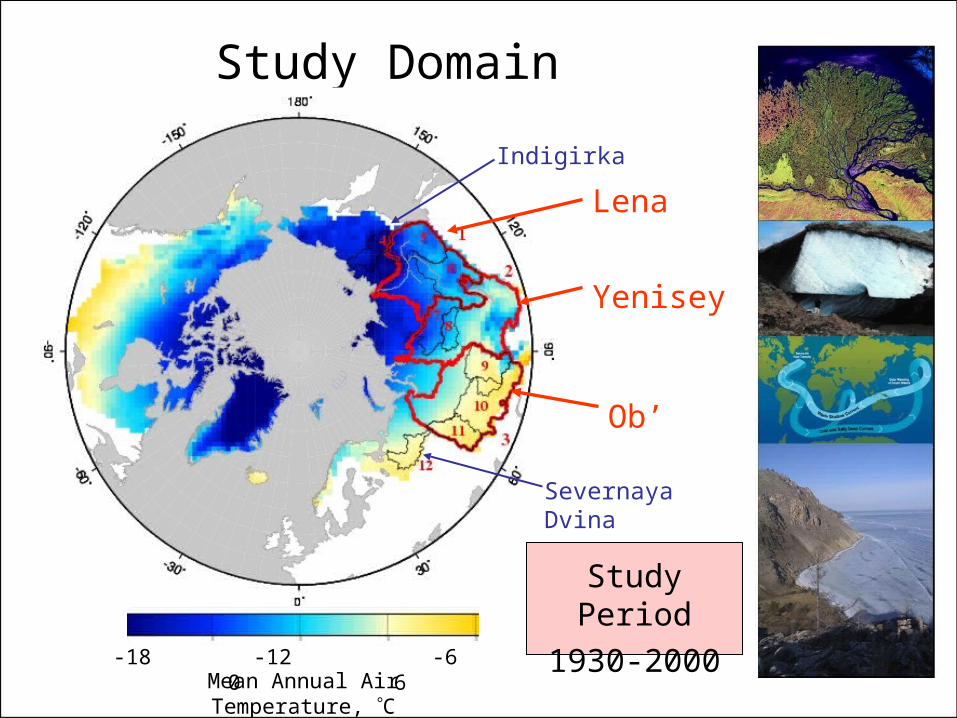
Study Domain

Mean Annual Air Temperature, C-18 -12 -6 0 6

Lena

Yenisey

Ob’

Study Period

1930-2000

Indigirka

Severnaya Dvina

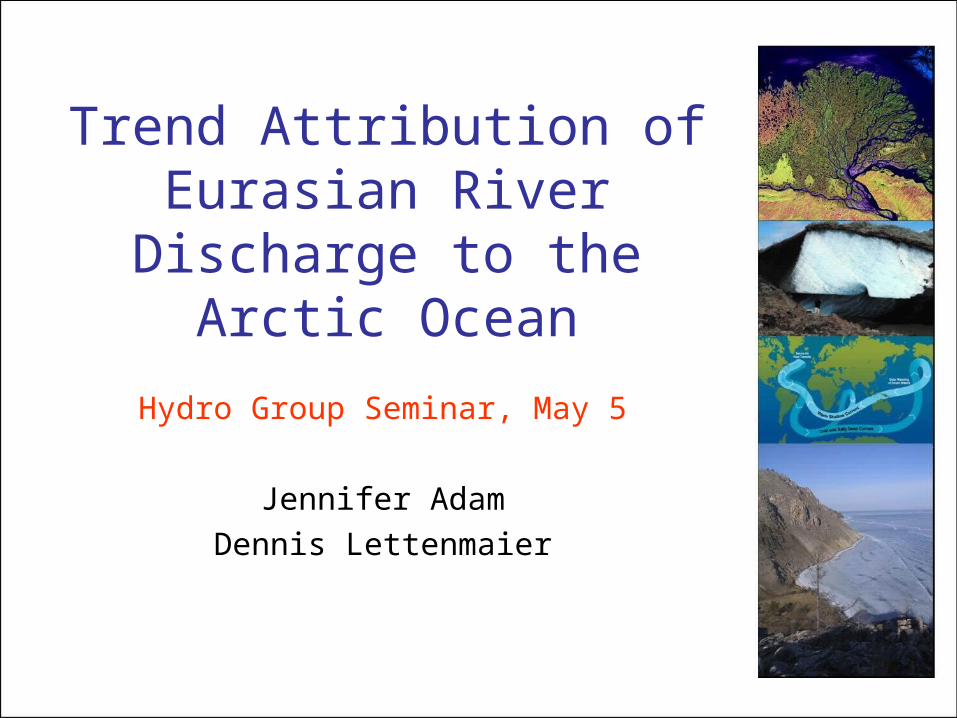
Observed Stream Flow Trends

• Discharge to Arctic Ocean from six largest Eurasian rivers is increasing, 1936 to 1998: +128 km3/yr (~7% increase)

• Most significant trends during the winter (low-flow) season

• Purpose of study: to investigate what is causing this

Dis

cha

rge,

km

3/y

r Annual trend for the 6 largest rivers

Peterson et al. 2002

J F M A M J J A S O N D

10

20

30

40

Dis

cha

rge,

m3/s

GRDCMonthly Means Ob’

1950 1960 1970 1980

Dis

cha

rge,

km

3

Winter Trend, Ob’

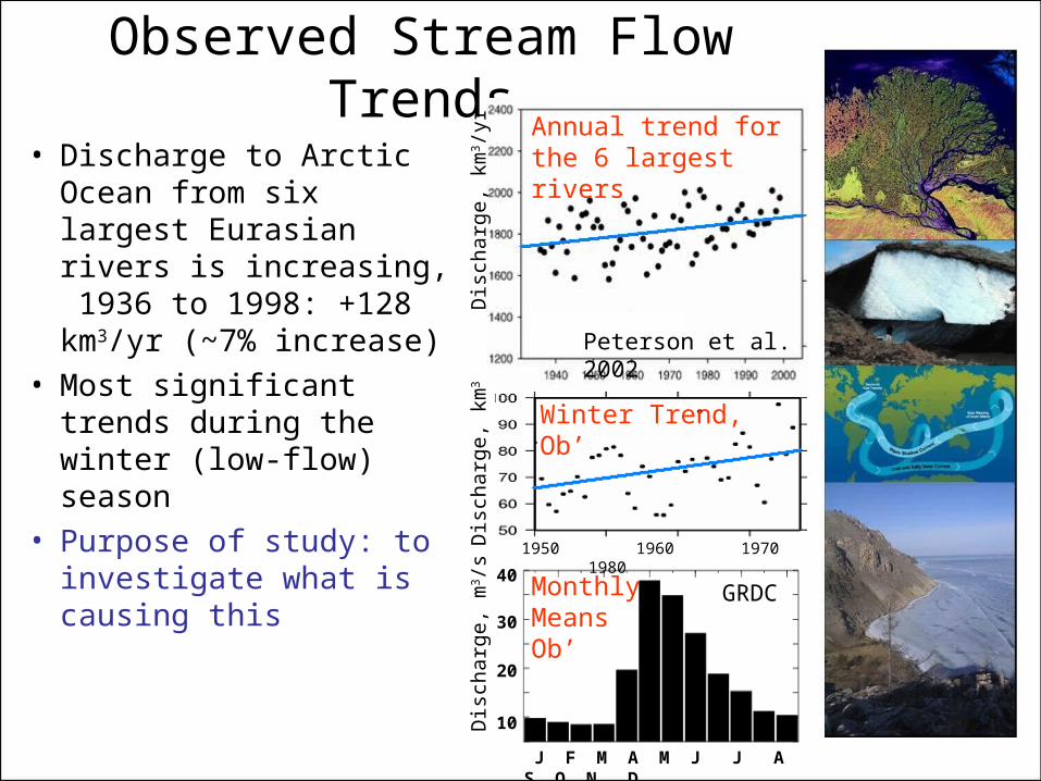
• Currently experiencing system-wide change: All subsystems affected!

– Rivers, temperature, precipitation, permafrost, snow, wetlands, glaciers, vegetation zonation, fire frequency, insect infestations…

Climate and the Arctic

• Implications to global climate:(1) Albedo feedback

(2) Greenhouse gas emissions/uptake

(3) Ocean circulation feedback

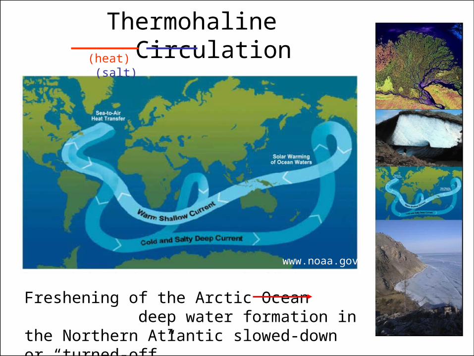
www.noaa.gov

Thermohaline Circulation(heat) (salt)

Freshening of the Arctic Ocean deep water formation in the Northern Atlantic slowed-down or “turned-off”

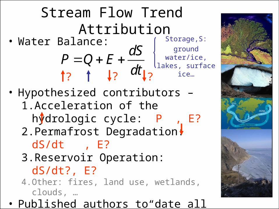
Stream Flow Trend Attribution

• Hypothesized contributors –1.Acceleration of the hydrologic cycle:

P , E?2.Permafrost Degradation: dS/dt , E?3.Reservoir Operation: dS/dt?, E? 4. Other: fires, land use, wetlands, clouds, …

• Published authors to date all say, “we don’t know”: McClelland et al. (2004), Berezovskaya et al. (2004), Pavelsky and Smith (2006)…

• Water Balance:dS

P Q Edt

Storage,S:

ground water/ice, lakes, surface

ice…

? ? ?

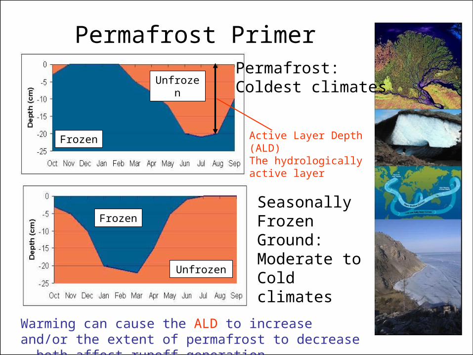
Permafrost Primer

Frozen

Frozen

Unfrozen

Unfrozen

Permafrost:Coldest climates

Seasonally Frozen Ground:Moderate to Cold climates

Active Layer Depth (ALD)The hydrologically active layer

Warming can cause the ALD to increase and/or the extent of permafrost to decrease – both affect runoff generation

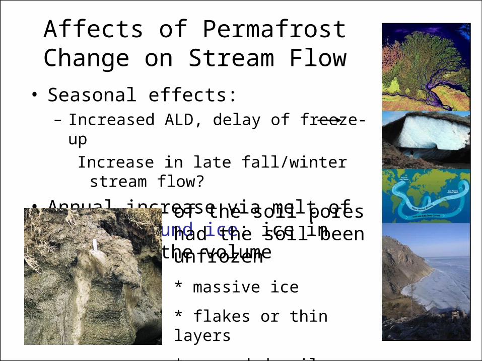
Affects of Permafrost Change on Stream Flow

• Seasonal effects:– Increased ALD, delay of freeze-up

Increase in late fall/winter stream flow?

• Annual increase via melt of excess ground ice: ice in excess of the volume

of the soil pores had the soil been unfrozen

* massive ice

* flakes or thin layers

* expanded soil pores

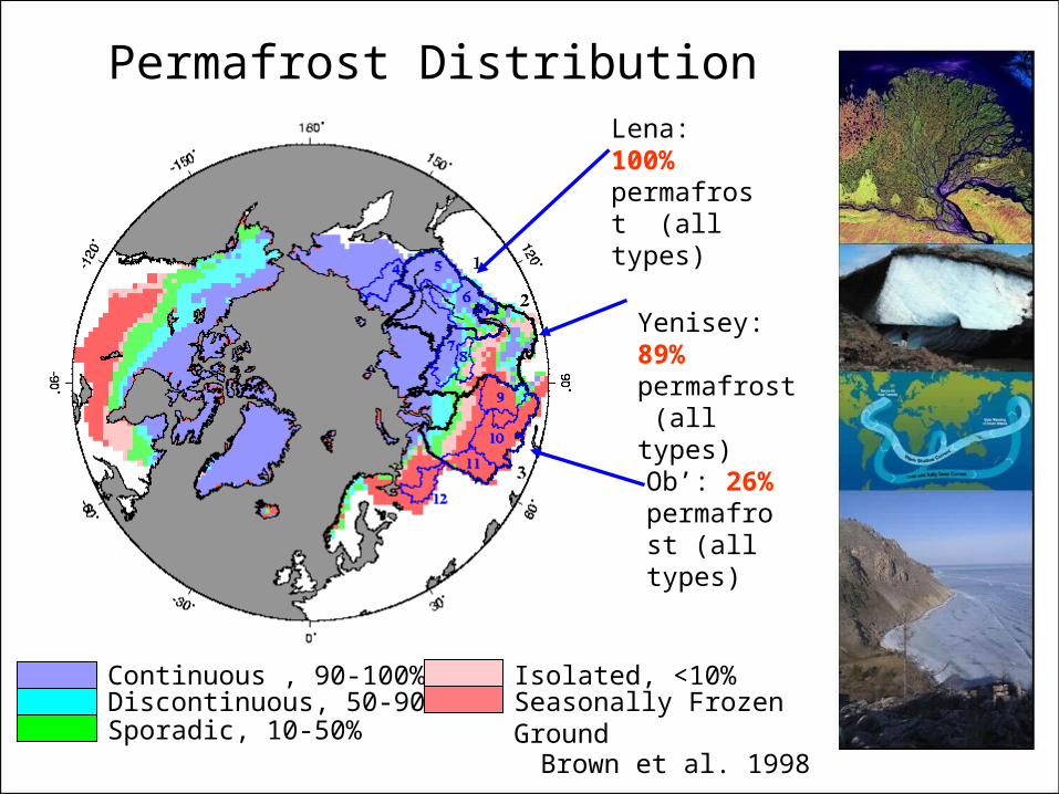
Lena: 100% permafrost (all types)

Yenisey: 89% permafrost (all types)

Ob’: 26% permafrost (all types)

Permafrost Distribution

Continuous , 90-100%Discontinuous, 50-90%Sporadic, 10-50%

Seasonally Frozen GroundIsolated, <10%

Brown et al. 1998

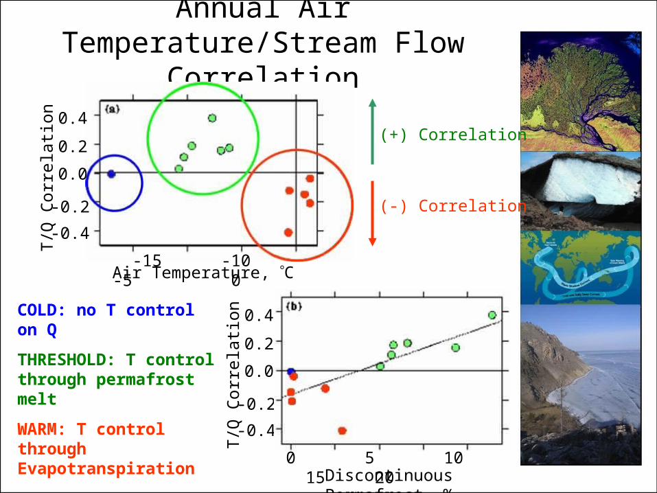
Annual Air Temperature/Stream Flow Correlation

Discontinuous Permafrost, %0 5 10 15 20

T/Q

Cor

rela

tion 0.4

0.2

0.0

-0.2

-0.4

-15 -10 -5 0Air Temperature, C

T/Q

Cor

rela

tion 0.4

0.2

0.0

-0.2

-0.4

(+) Correlation

(-) Correlation

COLD: no T control on Q

THRESHOLD: T control through permafrost melt

WARM: T control through Evapotranspiration

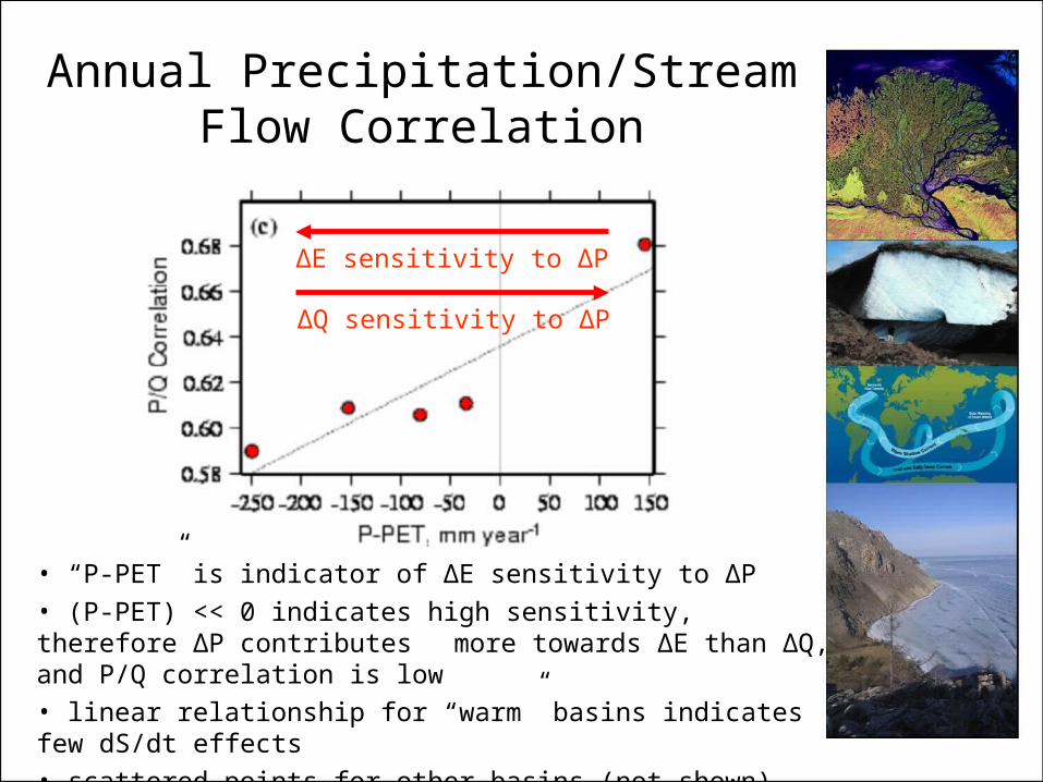
Annual Precipitation/Stream Flow Correlation

• “P-PET” is indicator of ΔE sensitivity to ΔP

• (P-PET) << 0 indicates high sensitivity, therefore ΔP contributes more towards ΔE than ΔQ, and P/Q correlation is low

• linear relationship for “warm” basins indicates few dS/dt effects

• scattered points for other basins (not shown) indicates more significant dS/dt effects

ΔE sensitivity to ΔP

ΔQ sensitivity to ΔP

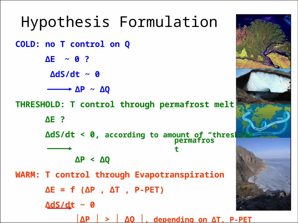
Hypothesis FormulationCOLD: no T control on Q

ΔE ~ 0 ?

ΔdS/dt ~ 0

ΔP ~ ΔQ

THRESHOLD: T control through permafrost melt

ΔE ?

ΔdS/dt < 0, according to amount of “threshold”

ΔP < ΔQ

WARM: T control through Evapotranspiration

ΔE = f (ΔP , ΔT , P-PET)

ΔdS/dt ~ 0

│ΔP │ > │ ΔQ │, depending on ΔT, P-PET

permafrost

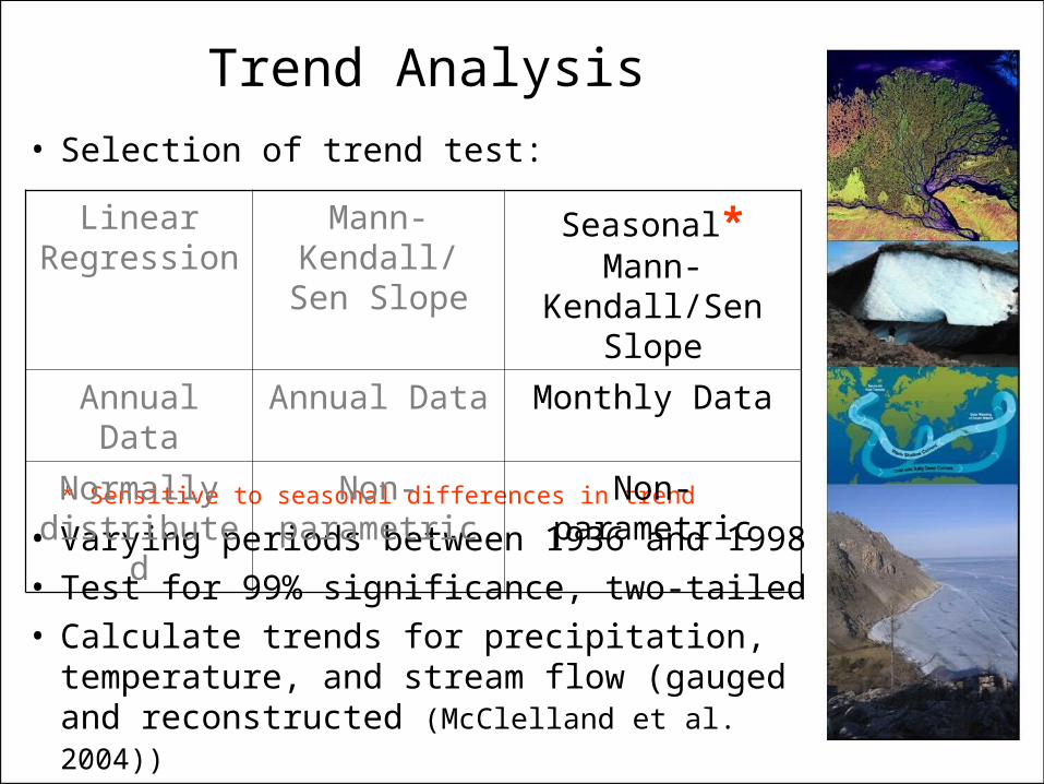
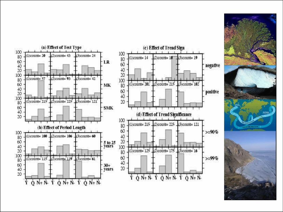
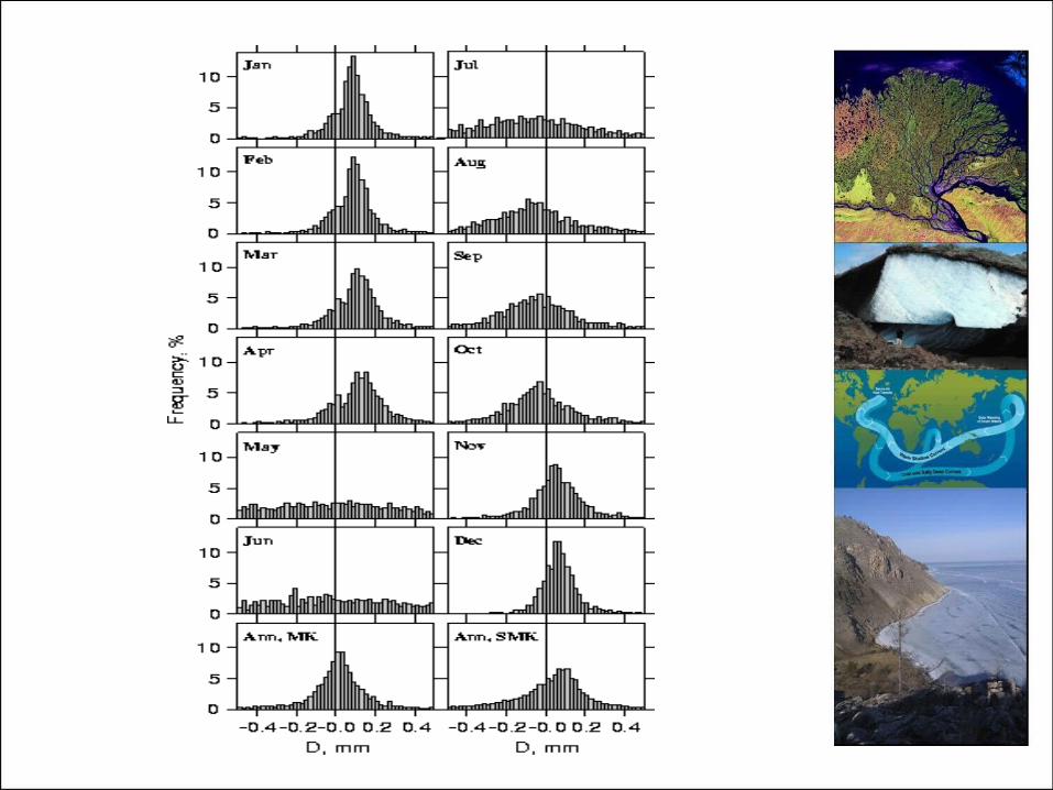
• Selection of trend test:

* Sensitive to seasonal differences in trend

• Varying periods between 1936 and 1998• Test for 99% significance, two-tailed• Calculate trends for precipitation,

temperature, and stream flow (gauged and reconstructed (McClelland et al. 2004))

Trend Analysis

Linear Regression

Mann-Kendall/ Sen Slope

Seasonal* Mann-Kendall/Sen

Slope

Annual Data Annual Data Monthly Data

Normally distributed

Non-parametric Non-parametric

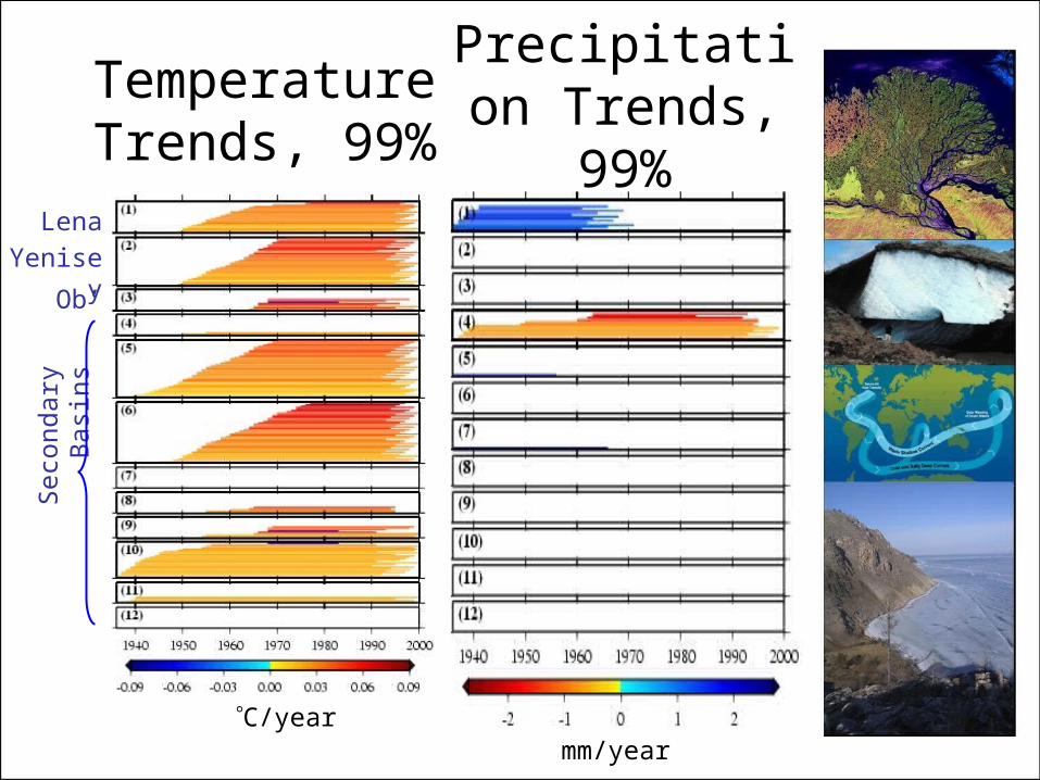
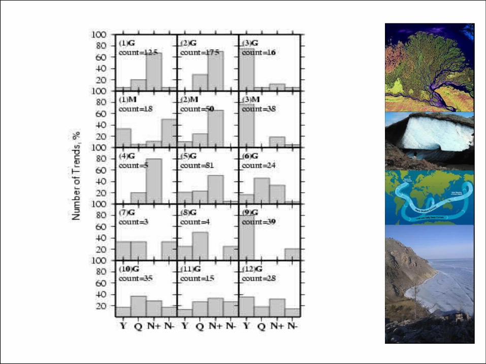
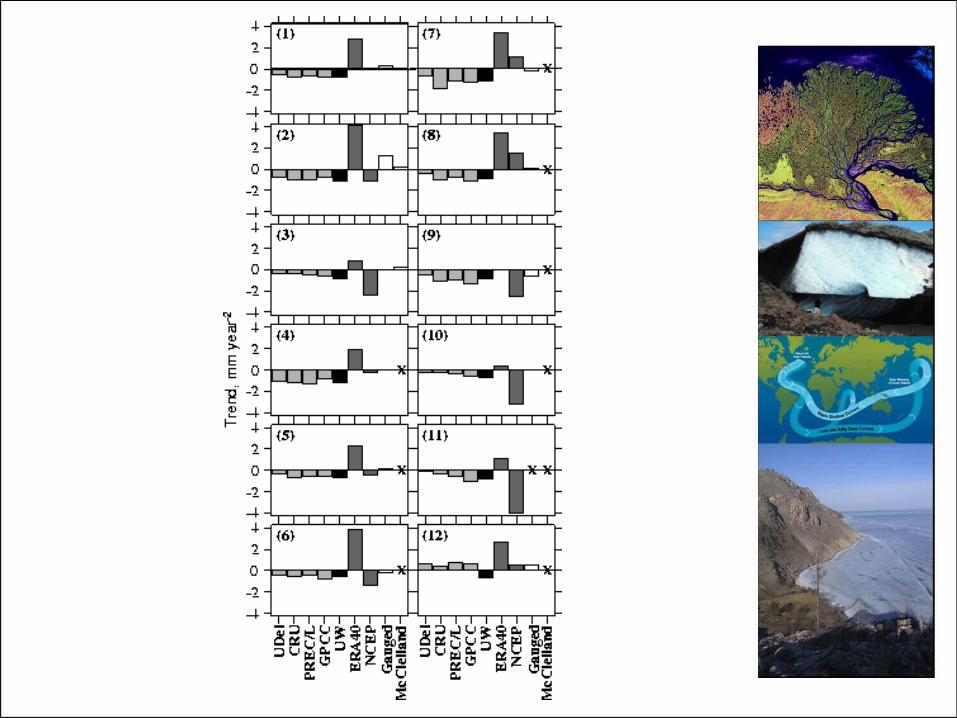
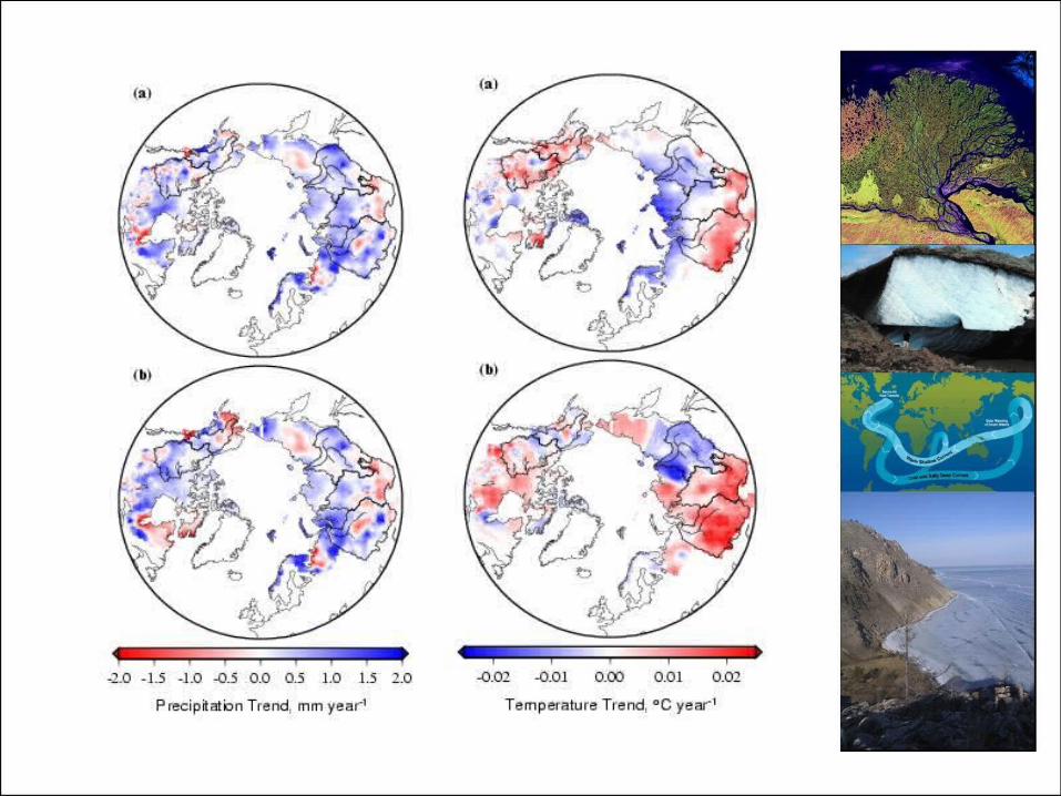
Temperature Trends, 99%

Precipitation Trends, 99%

mm/yearC/year

Lena

Yenisey

Ob’

Sec

onda

ry B

asin

s

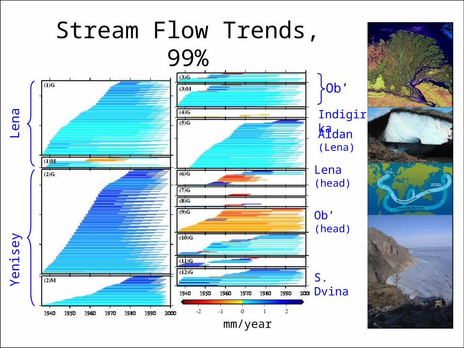
Stream Flow Trends, 99%

Len

a

Ob’

Ye

nise

y

Aldan (Lena)

Lena (head)

S. Dvina

Ob’ (head)

Indigirka

mm/year

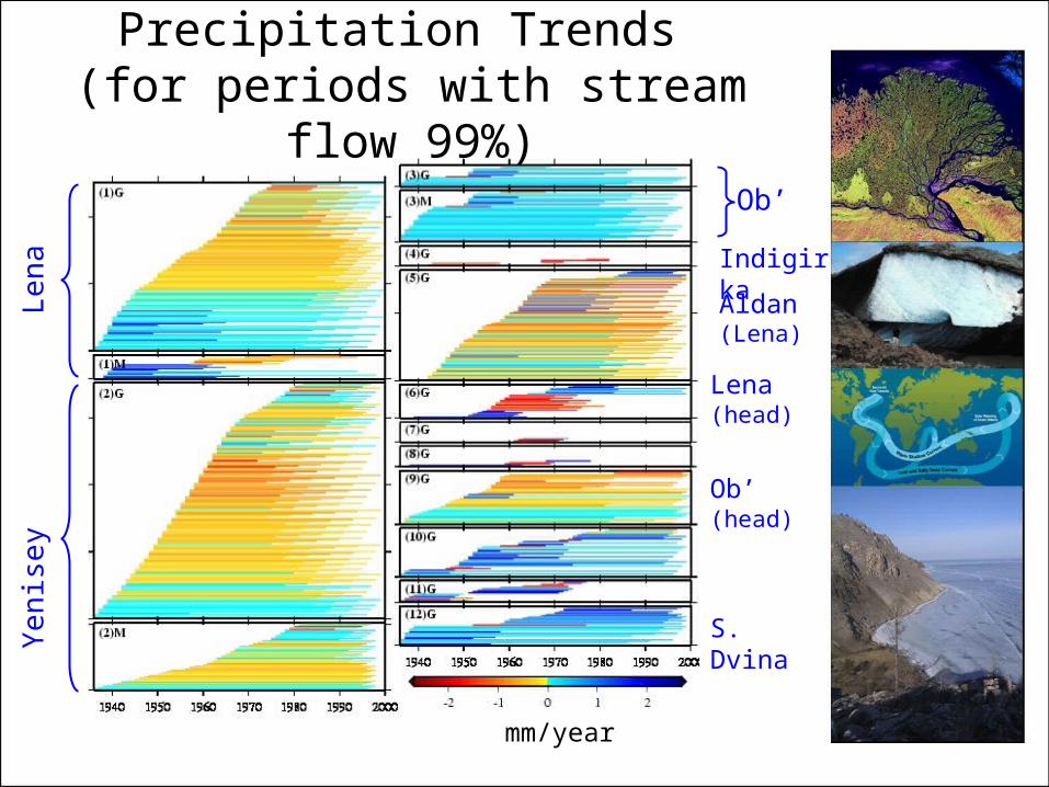
Precipitation Trends (for periods with stream flow 99%)

Len

a

Ob’

Ye

nise

y

Aldan (Lena)

Lena (head)

S. Dvina

Ob’ (head)

Indigirka

mm/year

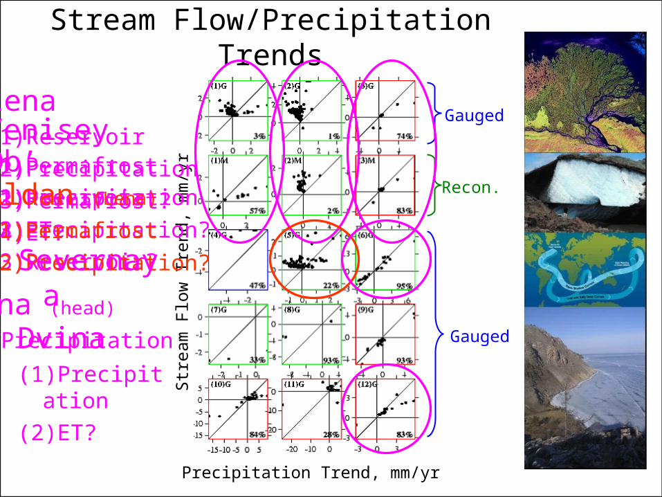
Str

eam

Flo

w T

rend

, m

m/y

r

Precipitation Trend, mm/yr

Stream Flow/Precipitation Trends

Gauged

Recon.

Gauged

Lena(1)Reservoir

(2)Precipitation

(3)Permafrost?

(4)ET?

Yenisey(1)Permafrost

(2)Reservoir

(3)Precipitation?

Ob’(1)Precipitation

(2)ET

(3)Reservoir?

Aldan (Lena)

(1)Permafrost

(2)Precipitation?

Lena (head)

(1)Precipitation

Severnaya

Dvina(1)Precipitation

(2)ET?

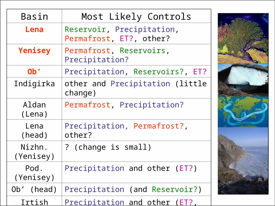
Basin Most Likely ControlsLena Reservoir, Precipitation, Permafrost, ET?,

other?

Yenisey Permafrost, Reservoirs, Precipitation?

Ob’ Precipitation, Reservoirs?, ET?

Indigirka other and Precipitation (little change)

Aldan (Lena) Permafrost, Precipitation?

Lena (head) Precipitation, Permafrost?, other?

Nizhn. (Yenisey)

? (change is small)

Pod. (Yenisey)

Precipitation and other (ET?)

Ob’ (head) Precipitation (and Reservoir?)

Irtish (Ob’) Precipitation and other (ET?, Reservoirs?)

Tobol (Ob’) ? (change is small)

S. Dvina Precipitation and other (ET?)

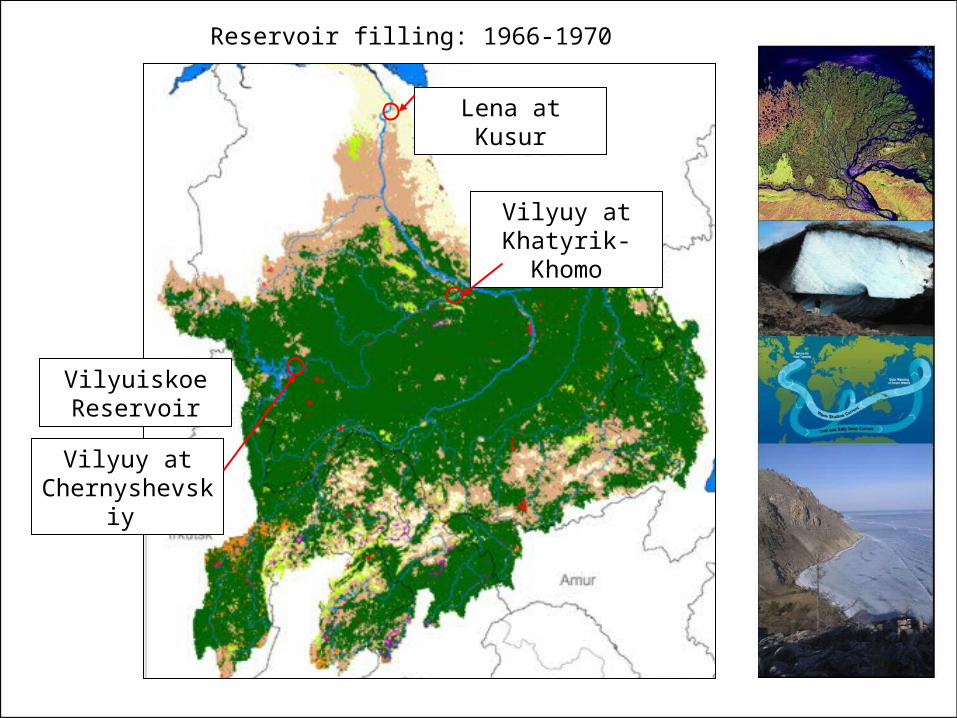
Lena at Kusur

Vilyuy at Khatyrik-Khomo

Vilyuy at Chernyshevskiy

Vilyuiskoe Reservoir

Reservoir filling: 1966-1970

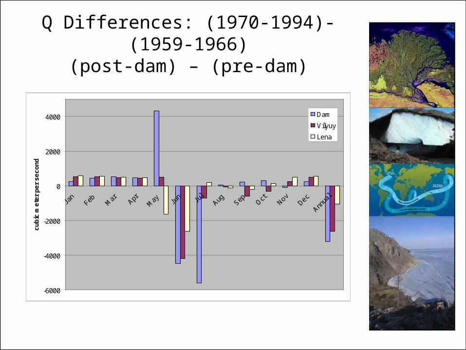
Q Differences: (1970-1994)-(1959-1966)(post-dam) – (pre-dam)

-6000

-4000

-2000

0

2000

4000

cu

bic

me

ter

pe

r s

ec

on

d

Dam

Vilyuy

Lena

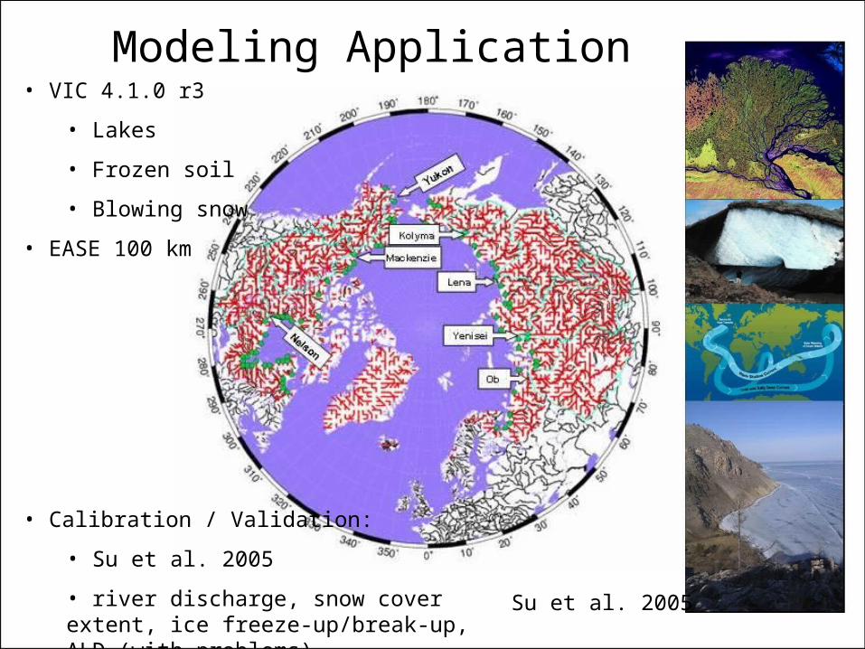
Modeling Application

Su et al. 2005

• VIC 4.1.0 r3

• Lakes

• Frozen soil

• Blowing snow

• EASE 100 km

• Calibration / Validation:

• Su et al. 2005

• river discharge, snow cover extent, ice freeze-up/break-up, ALD (with problems)

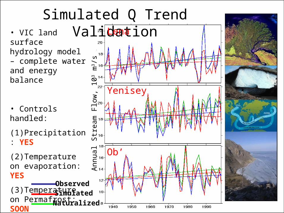
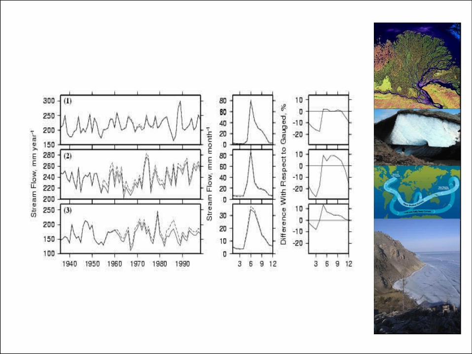
Simulated Q Trend ValidationLena

Yenisey

Ob’

ObservedSimulated

Naturalized

• VIC land surface hydrology model – complete water and energy balance

• Controls handled:

(1)Precipitation: YES

(2)Temperature on evaporation: YES

(3)Temperature on Permafrost: SOON

(4) Reservoirs: NO

Ann

ual S

trea

m F

low

, 10

3 m

3 /s

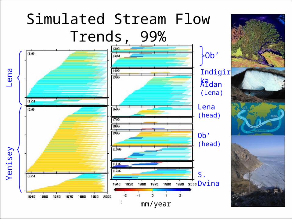
Simulated Stream Flow Trends, 99%

Len

a

Ob’

Ye

nise

y

Aldan (Lena)

Lena (head)

S. Dvina

Ob’ (head)

Indigirka

mm/year

Observed Stream Flow Trends, 99%

Len

a

Ob’

Ye

nise

y

Aldan (Lena)

Lena (head)

S. Dvina

Ob’ (head)

Indigirka

mm/year

Gauged

Recon.

Gauged

Obs

erve

d T

rend

, m

m/y

r

Simulated Trend, mm/yr

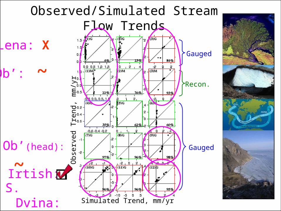
Observed/Simulated Stream Flow Trends

Lena: X

Ob’: ~

Ob’(head): ~Irtish:

S. Dvina: ~

Study Domain

Mean Annual Air Temperature, C-18 -12 -6 0 6

Lena

Yenisey

Ob’

Study Period

1930-2000

Indigirka

Severnaya Dvina

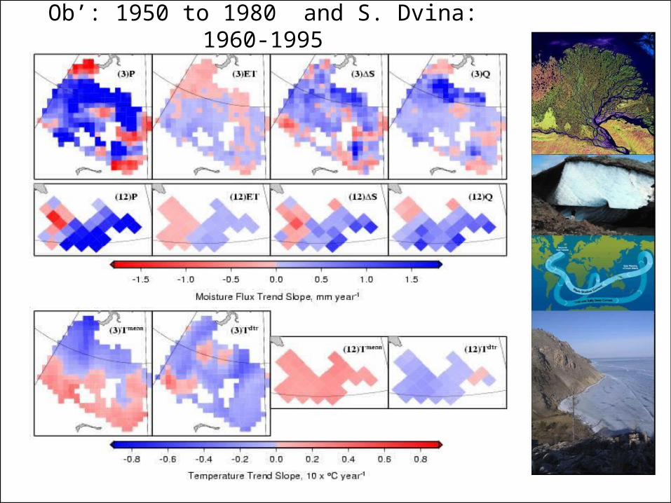
Ob’: 1950 to 1980 and S. Dvina: 1960-1995

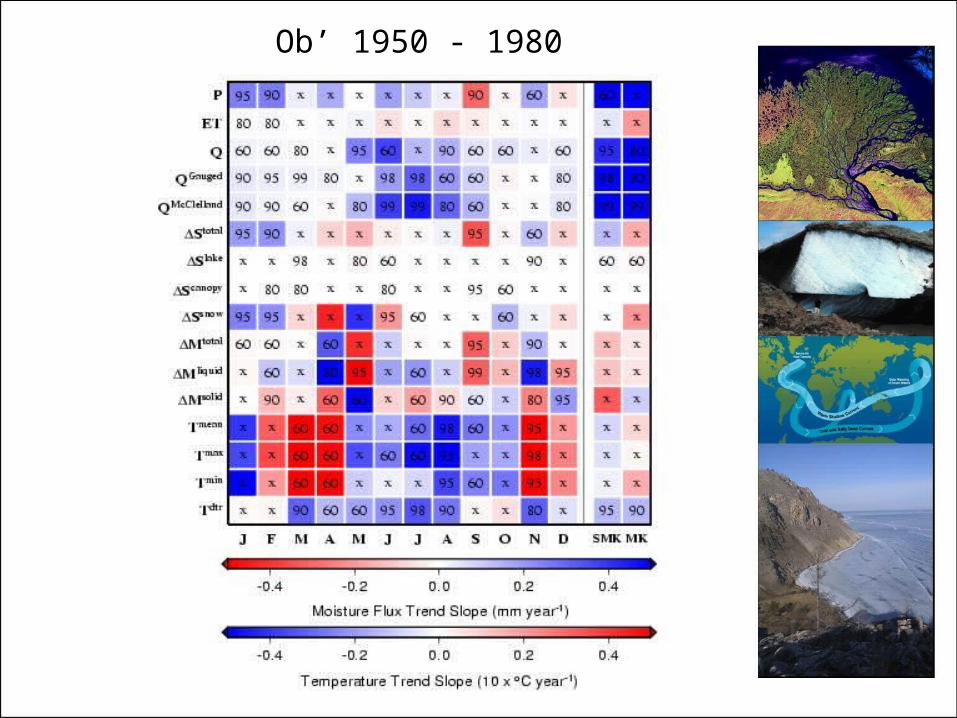
Ob’ 1950 - 1980

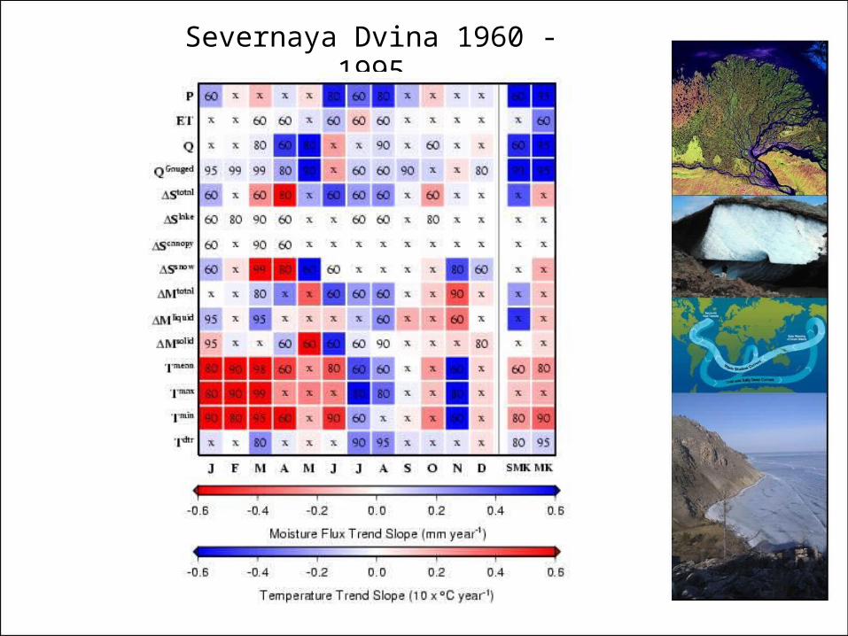
Severnaya Dvina 1960 - 1995

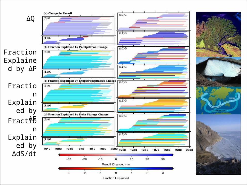
ΔQ

Fraction Explained

by ΔP

Fraction Explained

by ΔE

Fraction Explained by ΔdS/dt

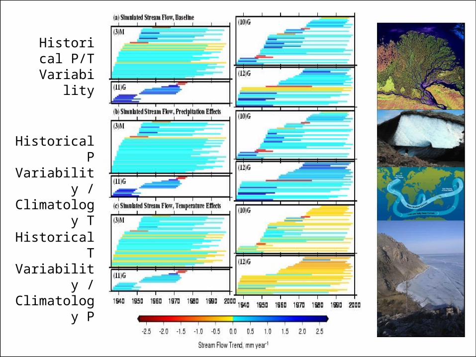
Historical P/T

Variability

Historical P Variability /

Climatology T

Historical T Variability /

Climatology P

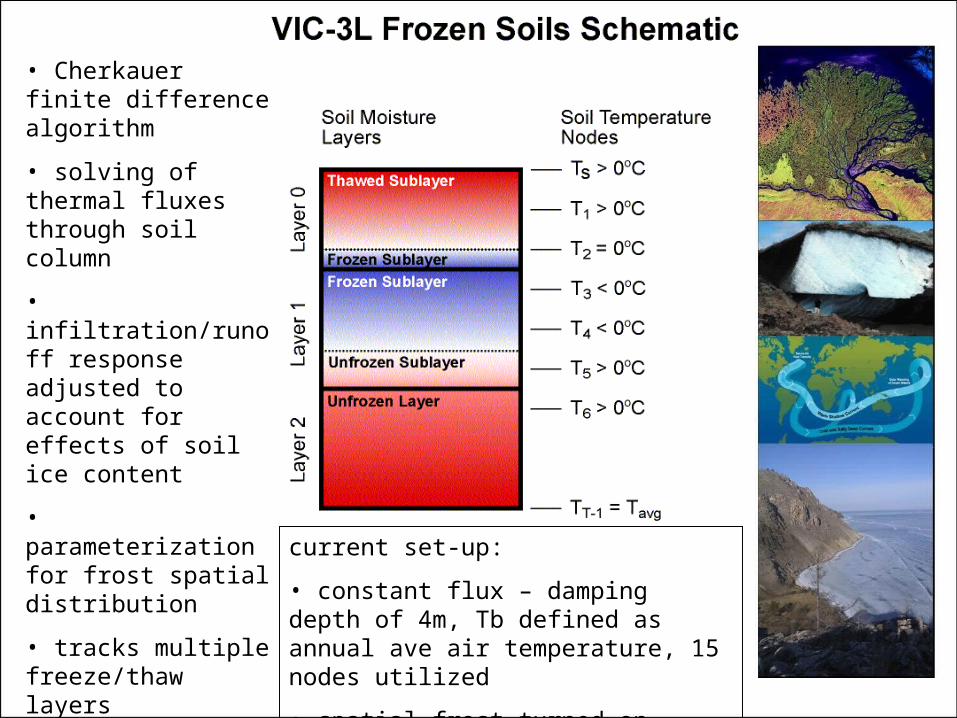
• Cherkauer finite difference algorithm

• solving of thermal fluxes through soil column

• infiltration/runoff response adjusted to account for effects of soil ice content

• parameterization for frost spatial distribution

• tracks multiple freeze/thaw layers

• can use either “no flux” or “constant flux” bottom boundary

current set-up:

• constant flux – damping depth of 4m, Tb defined as annual ave air temperature, 15 nodes utilized

• spatial frost turned on

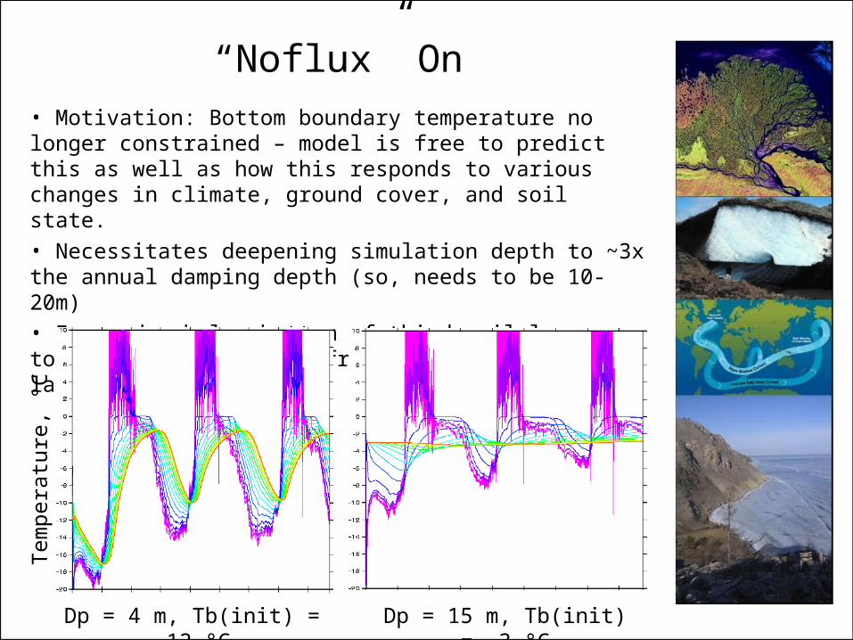
“Noflux” On• Motivation: Bottom boundary temperature no longer constrained – model is free to predict this as well as how this responds to various changes in climate, ground cover, and soil state.

• Necessitates deepening simulation depth to ~3x the annual damping depth (so, needs to be 10-20m)

• For nodes below bottom of third soil layer, total moisture derived from bottom soil moisture layer

Dp = 4 m, Tb(init) = -12 °C Dp = 15 m, Tb(init) = -3 °C

Tem

pera

ture

, °C

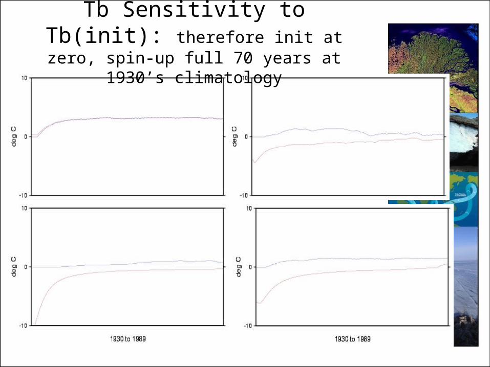
Tb Sensitivity to Tb(init): therefore init at zero, spin-up full 70 years at 1930’s

climatology

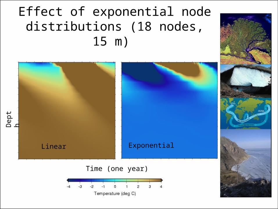
Effect of exponential node distributions (18 nodes, 15 m)

Time (one year)

Dep

th

Linear Exponential

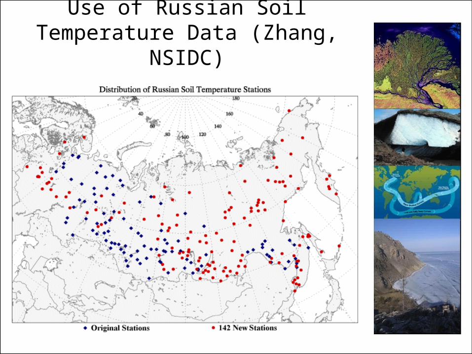
Use of Russian Soil Temperature Data (Zhang, NSIDC)

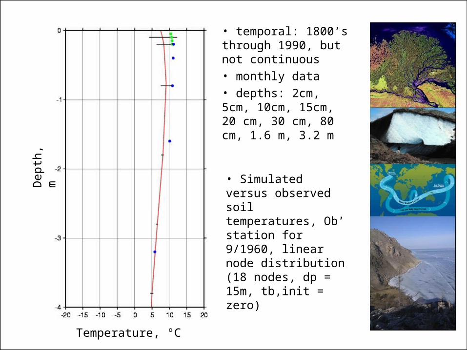
Dep

th,

m

Temperature, °C

• temporal: 1800’s through 1990, but not continuous

• monthly data

• depths: 2cm, 5cm, 10cm, 15cm, 20 cm, 30 cm, 80 cm, 1.6 m, 3.2 m

• Simulated versus observed soil temperatures, Ob’ station for 9/1960, linear node distribution (18 nodes, dp = 15m, tb,init = zero)

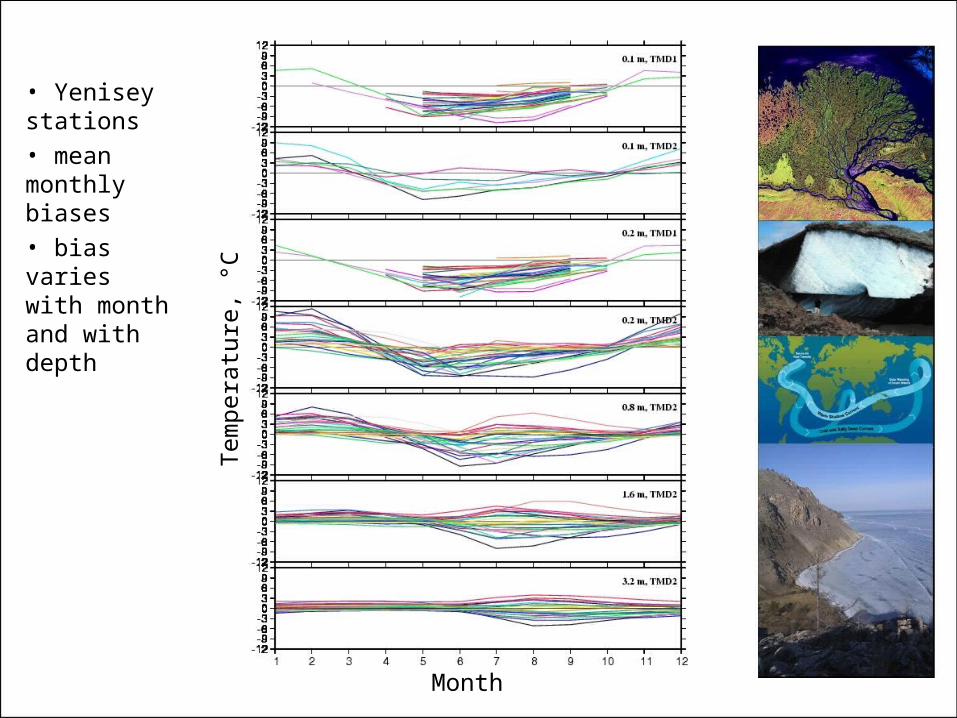
Month

Tem

pera

ture

, °C

• Yenisey stations

• mean monthly biases

• bias varies with month and with depth

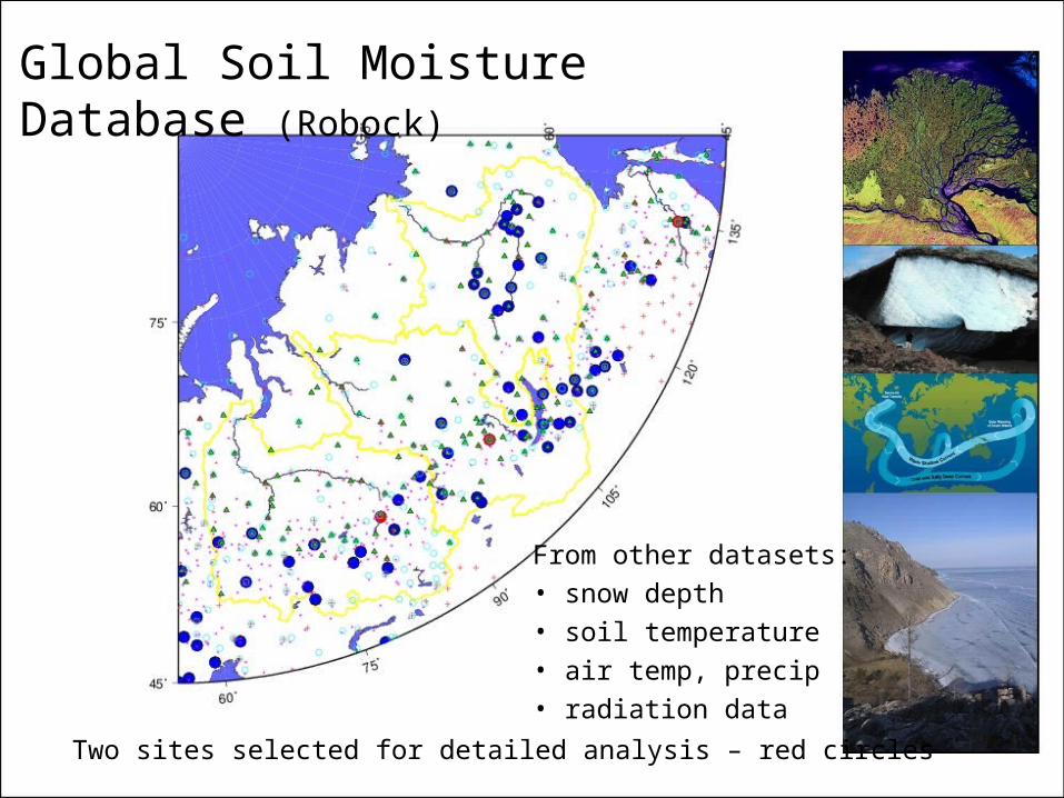
Global Soil Moisture Database (Robock)

From other datasets:

• snow depth

• soil temperature

• air temp, precip

• radiation data

Two sites selected for detailed analysis – red circles

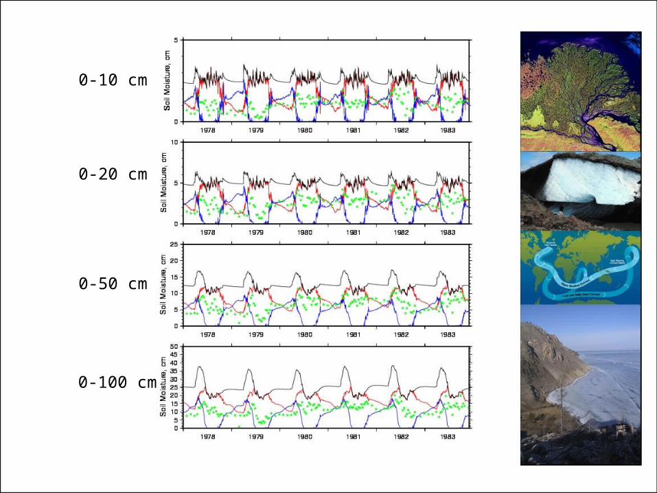
0-10 cm

0-20 cm

0-50 cm

0-100 cm

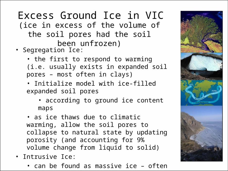
Excess Ground Ice in VIC(ice in excess of the volume of the soil

pores had the soil been unfrozen)

• Segregation Ice: • the first to respond to warming (i.e. usually exists in expanded soil pores – most often in clays)• Initialize model with ice-filled expanded soil pores

• according to ground ice content maps• as ice thaws due to climatic warming, allow the soil pores to collapse to natural state by updating porosity (and accounting for 9% volume change from liquid to solid)

• Intrusive Ice:• can be found as massive ice – often the last and slowest response to warming• add a soil layer of pure ice to VIC

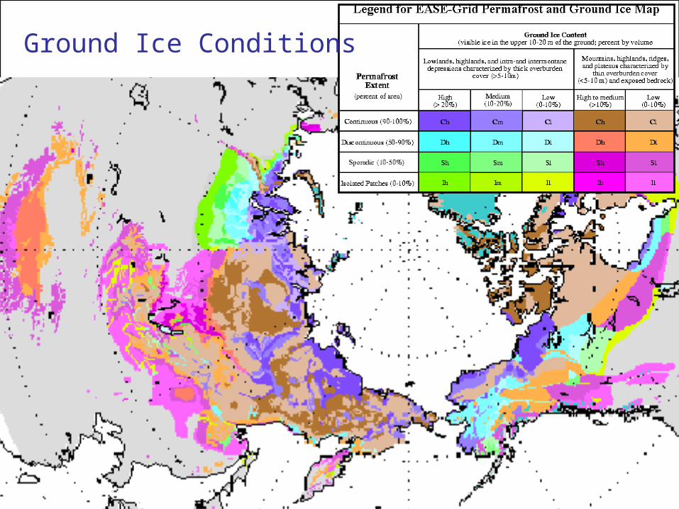
Ground Ice Conditions

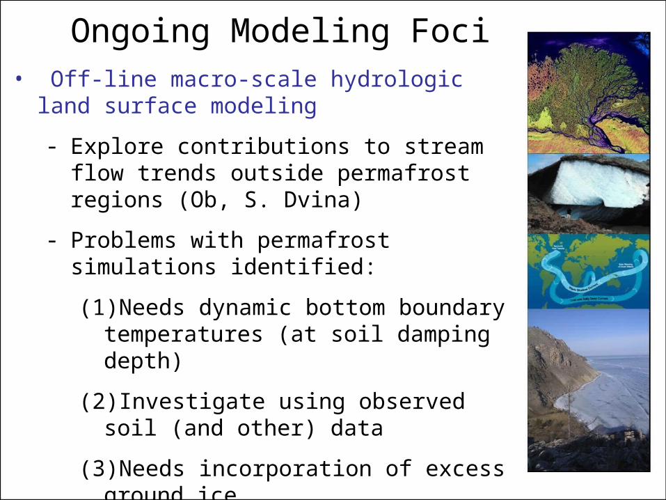
Ongoing Modeling Foci• Off-line macro-scale hydrologic land surface

modeling

- Explore contributions to stream flow trends outside permafrost regions (Ob, S. Dvina)

- Problems with permafrost simulations identified:

(1)Needs dynamic bottom boundary temperatures (at soil damping depth)

(2)Investigate using observed soil (and other) data

(3)Needs incorporation of excess ground ice

• Stream Flow Predictions – using downscaled GCM output

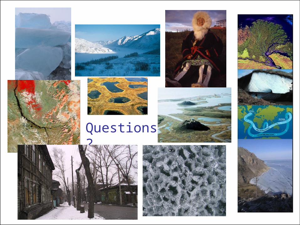
Questions?

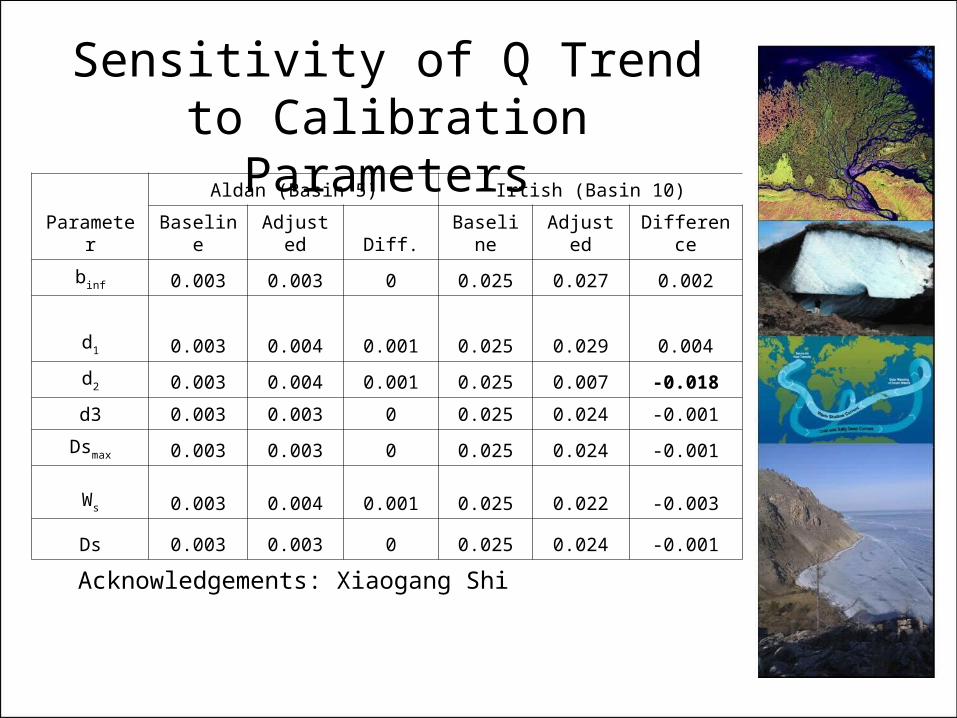
Parameter

Aldan (Basin 5) Irtish (Basin 10)

Baseline Adjusted Diff. Baseline Adjusted Difference

binf 0.003 0.003 0 0.025 0.027 0.002

d1 0.003 0.004 0.001 0.025 0.029 0.004

d2 0.003 0.004 0.001 0.025 0.007 -0.018

d3 0.003 0.003 0 0.025 0.024 -0.001

Dsmax 0.003 0.003 0 0.025 0.024 -0.001

Ws 0.003 0.004 0.001 0.025 0.022 -0.003

Ds 0.003 0.003 0 0.025 0.024 -0.001

Acknowledgements: Xiaogang Shi

Sensitivity of Q Trend to Calibration Parameters

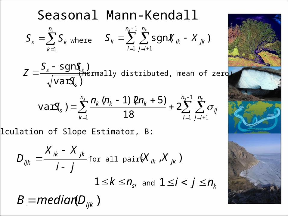
sn

kks SS

1

1

1 1

)sgn(k kn

i

n

ijjkikk XXS

)var(

)sgn(

s

ss

S

SSZ

1

1 11

218

)52)(1()var(

s ss n

i

n

ijij

n

k

kkks

nnnS

ji

XXD jkikijk

for all pairs ),( jkik XX

(normally distributed, mean of zero)

snk 1 , and knji 1

. )( ijkDmedianB

where

Seasonal Mann-Kendall

Calculation of Slope Estimator, B:

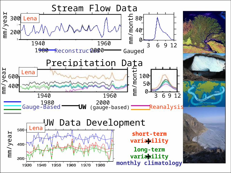
Stream Flow Data

UW Data Development

mm

/yea

r

Lena

monthly climatology

long-term variability

short-term variability

++

Reconstructed Gauged 1940 1960 1980 2000

Lena300

200mm

/yea

r

80

40

0mm

/mon

th

3 6 9 12

Precipitation DataLena

1940 1960 1980 2000

600

400

mm

/yea

r

100500m

m/m

onth

Gauge-Based UW (gauge-based) Reanalysis

3 6 9 12

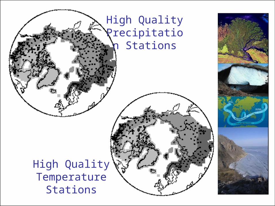
High Quality Precipitation

Stations

High Quality Temperature

Stations

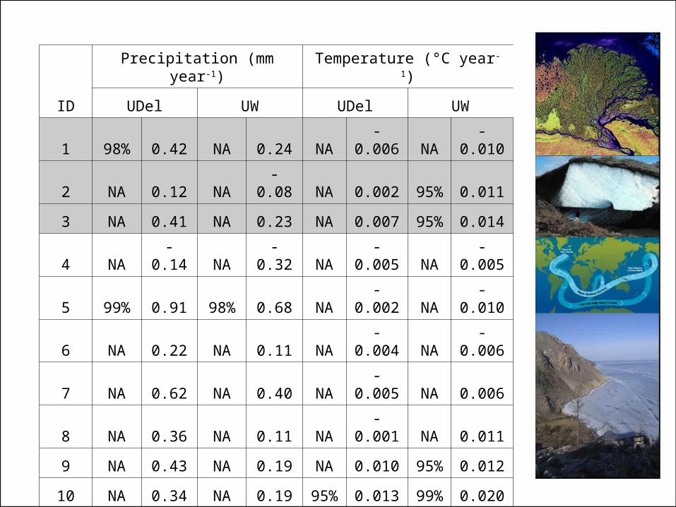
ID

Precipitation (mm year-1) Temperature (°C year-1)

UDel UW UDel UW

1 98% 0.42 NA 0.24 NA -0.006 NA -0.010

2 NA 0.12 NA -0.08 NA 0.002 95% 0.011

3 NA 0.41 NA 0.23 NA 0.007 95% 0.014

4 NA -0.14 NA -0.32 NA -0.005 NA -0.005

5 99% 0.91 98% 0.68 NA -0.002 NA -0.010

6 NA 0.22 NA 0.11 NA -0.004 NA -0.006

7 NA 0.62 NA 0.40 NA -0.005 NA 0.006

8 NA 0.36 NA 0.11 NA -0.001 NA 0.011

9 NA 0.43 NA 0.19 NA 0.010 95% 0.012

10 NA 0.34 NA 0.19 95% 0.013 99% 0.020

11 NA 0.41 NA 0.34 NA 0.010 90% 0.014

12 NA 0.12 NA 0.28 NA -0.003 NA 0.001

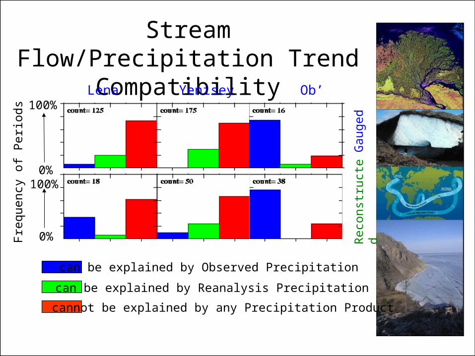
Stream Flow/Precipitation Trend Compatibility

can be explained by Observed Precipitation

can be explained by Reanalysis Precipitation

cannot be explained by any Precipitation Product

Lena Ob’Yenisey

0%

100%

Gau

ged

Rec

onst

ruct

ed

0%

100%

Fre

quen

cy o

f P

erio

ds