PAPER • OPEN ACCESS

Truncation identities for the small polaron fusionhierarchyTo cite this article: André M Grabinski and Holger Frahm 2013 New J. Phys. 15 043026

 

View the article online for updates and enhancements.

You may also likeThird quantization: a general method tosolve master equations for quadratic openFermi systemsTomaž Prosen

-

Paramagnetic dust particles in rf-plasmaswith weak external magnetic fieldsMarian Puttscher and André Melzer

-

Andreev reflection without Fermi surfacealignment in high-Tc van der WaalsheterostructuresParisa Zareapour, Alex Hayat, Shu Yang FZhao et al.

-

Recent citationsGraded off-diagonal Bethe ansatz solutionof the SU(2|2) spin chain model withgeneric integrable boundariesXiaotian Xu et al

-

The stability of hole-dopedantiferromagnetic state in a two-orbitalmodelDheeraj Kumar Singh et al

-

On the Bethe states of the one-dimensional supersymmetric t J modelwith generic open boundariesPei Sun et al

-

This content was downloaded from IP address 168.149.121.250 on 12/11/2021 at 05:17

Truncation identities for the small polaronfusion hierarchy

Andre M Grabinski and Holger Frahm1

Institut fur Theoretische Physik, Leibniz Universitat Hannover, Appelstraße 2,D-30167 Hannover, GermanyE-mail: frahm@itp.uni-hannover.de

New Journal of Physics 15 (2013) 043026 (31pp)Received 28 November 2012Published 17 April 2013Online at http://www.njp.org/doi:10.1088/1367-2630/15/4/043026

Abstract. We study a one-dimensional lattice model of interacting spinlessfermions. This model is integrable for both periodic and open boundaryconditions; the latter case includes the presence of Grassmann valued non-diagonal boundary fields breaking the bulk U (1) symmetry of the model.Starting from the embedding of this model into a graded Yang–Baxter algebra,an infinite hierarchy of commuting transfer matrices is constructed by meansof a fusion procedure. For certain values of the coupling constant related toanisotropies of the underlying vertex model taken at roots of unity, this hierarchyis shown to truncate giving a finite set of functional equations for the spectrumof the transfer matrices. For generic coupling constants, the spectral problemis formulated in terms of a functional (or TQ-)equation which can be solvedby Bethe ansatz methods for periodic and diagonal open boundary conditions.Possible approaches for the solution of the model with generic non-diagonalboundary fields are discussed.

1 Author to whom any correspondence should be addressed.

Content from this work may be used under the terms of the Creative Commons Attribution 3.0 licence.Any further distribution of this work must maintain attribution to the author(s) and the title of the work, journal

citation and DOI.

New Journal of Physics 15 (2013) 0430261367-2630/13/043026+31$33.00 © IOP Publishing Ltd and Deutsche Physikalische Gesellschaft

2

Contents

1. Introduction 22. The small polaron as a fundamental integrable model 3

2.1. Construction within the quantum inverse scattering method framework . . . . . 42.2. Asymptotic behavior of the periodic boundary conditions (PBC) transfer matrix 5

3. Fusion of the R-matrix in auxiliary space 63.1. General construction of higher fused R-matrices . . . . . . . . . . . . . . . . . 73.2. Fusion hierarchy for super transfer matrices . . . . . . . . . . . . . . . . . . . 8

4. TQ-equations for PBC 85. Truncation of the PBC fusion hierarchy 10

5.1. R-matrix truncation . . . . . . . . . . . . . . . . . . . . . . . . . . . . . . . . 105.2. Super transfer matrix truncation . . . . . . . . . . . . . . . . . . . . . . . . . 10

6. The small polaron with open boundary conditions (OBC) 116.1. Reflection algebras and boundary matrices . . . . . . . . . . . . . . . . . . . . 116.2. Properties of the OBC transfer matrix . . . . . . . . . . . . . . . . . . . . . . 136.3. Fusion of the boundary matrices . . . . . . . . . . . . . . . . . . . . . . . . . 146.4. Fusion hierarchy for OBC . . . . . . . . . . . . . . . . . . . . . . . . . . . . 15

7. TQ-equations for OBC 168. Truncation of the OBC fusion hierarchy 17

8.1. K -matrix truncation . . . . . . . . . . . . . . . . . . . . . . . . . . . . . . . . 188.2. OBC super transfer matrix truncation . . . . . . . . . . . . . . . . . . . . . . . 18

9. Summary and conclusion 20Acknowledgments 21Appendix A. Graded vector spaces 21Appendix B. Relation to Bracken’s dual reflection algebra 23Appendix C. Algebraic Bethe ansatz for diagonal boundaries 25Appendix D. Super quantum determinants 26Appendix E. Transformation matrices 28References 30

1. Introduction

The small polaron model provides an effective description of the behavior of an additionalelectron in a polar crystal [1, 2]. In one spatial dimension, this lattice system of interactingspinless fermions can be constructed within the framework of the quantum inverse scatteringmethod [3] allowing us to compute the excitation spectrum by Bethe ansatz techniques, seee.g. [4, 5]. By means of a graded generalization [6–8] of Sklyanin’s reflection algebra [9], itwas possible to provide the small polaron model with open boundary conditions (OBC) whilekeeping its integrability intact. These integrable boundary conditions are encoded in c-numbervalued 2× 2-matrix solutions to the reflection equations [10–12].

Diagonal boundary matrices correspond to boundary chemical potentials in theHamiltonian. In this case the small polaron model is equivalent to the spin-1/2 XXZ Heisenberg

New Journal of Physics 15 (2013) 043026 (http://www.njp.org/)

3

chain with boundary magnetic fields by means of a Jordan–Wigner transformation, similarlyas in the case of periodic boundary conditions (PBC) where this equivalence holds up to aboundary twist depending on the particle number [4, 13]. As a consequence, the spectrumof the open small polaron model can be obtained using Bethe ansatz methods [13–15]. Forgeneral non-diagonal solutions to the reflection equations, this equivalence does not hold asa consequence of the non-local nature of the Jordan–Wigner transformation. Furthermore, theunderlying grading implies that solutions to the reflection equations for the small polaron modelare super matrices [16]. In the corresponding Hamiltonian, the resulting additional boundaryterms do not conserve particle number and have anti-commuting scalars, i.e. odd Grassmannnumbers, as amplitudes. The fact that the U (1) symmetry of the model is broken implies thatin general there is no simple eigenstate (e.g. the Fock vacuum) of the model that can be usedas a reference state for the algebraic Bethe ansatz. Therefore, alternative approaches such asfunctional Bethe ansatz methods have to be employed to analyze the spectrum of the model.This situation is, in fact, very similar to the case of non-diagonal boundary magnetic fields in thespin-1/2 Heisenberg chains: in the approaches used so far the solution of the spectral problemrelies on constraints between the boundary fields at the two ends of the chain or restrictions onthe anisotropy, or it is limited to small finite systems thereby reducing their usefulness to studythis system in the thermodynamic limit [17–25].

In a previous publication [26] we have investigated the applicability of Bethe ansatzmethods in the simpler case of a model of free fermions with similar open boundaryconditions. We found that for a certain class of non-diagonal boundary super matrices, a unitarytransformation on the auxiliary space allowed for an exact solution of the free fermion model.Furthermore, the functional equations obtained there could be easily generalized to describe thespectrum of the model for arbitrary non-diagonal boundary fields. Unfortunately, this approachcannot be applied directly to the small polaron model.

In this paper we initiate a study as to whether the nilpotency of the off-diagonal boundaryparameters in a graded model allows us to bypass some of the problems arising in the case of thespin-1/2 XXZ chain with non-diagonal boundary fields. Following ideas [17, 20] developed inthe context of the spin-1/2 XXZ Heisenberg chain and later generalized to the XYZ chain [27]and integrable higher spin XXZ models [28], we adapt the fusion procedure [29–31] for thetransfer matrix of the quantum chain to the graded case of the small polaron model. We derivethe fusion hierarchy of functional equations for a commuting family of transfer matrices forthe small polaron model. Assuming the existence of a certain limit, we formulate the spectralproblem of this model for periodic and general open boundary conditions in terms of functionalTQ-equations. For periodic and diagonal open boundary conditions, these equations are shownto coincide with the known result obtained from using the algebraic Bethe ansatz. For specialvalues of the interaction parameter related to roots of unity of the anisotropy parameter, wederive truncation identities for the fusion of the relevant objects, in particular the transfermatrices. Using these identities the fusion hierarchy reduces to a set of relations between finitelymany quantities.

2. The small polaron as a fundamental integrable model

Some materials exhibit a strong electron–phonon coupling that considerably reduces themobility of electrons within the conduction band. This interaction may be regarded as anincrease of the electron’s effective mass, thus giving rise to quasi-particles called polarons.

New Journal of Physics 15 (2013) 043026 (http://www.njp.org/)

4

If the electron is essentially trapped at a single lattice site, the corresponding quasi-particle issaid to be a small polaron. In this case, electron transport occurs either by thermally activatedhopping (at high temperatures) or by tunneling (at low temperatures).

In the case of PBC the N -site small polaron model is characterized by the Hamiltonian

H PBC=

N∑j=1

H j, j+1 with HN ,N+1 ≡ HN ,1 (2.1)

with a Hamiltonian density H j, j+1 defined as

H j, j+1 =−t(

c†j+1c j + c†

j c j+1

)+ V

(n j+1n j + n j+1n j

), (2.2)

where c†k and ck label the creation, respectively annihilation, operators of spinless fermions

at site k, which are subject to the anticommutation relations [c†`, ck]+ = δ`k . Moreover, it is

convenient to define number operators nk ≡ c†kck = 1− nk . In this context, the parameters t

and V may be interpreted as hopping amplitude and density–density interaction strength,respectively.

2.1. Construction within the quantum inverse scattering method framework

The small polaron model can be associated with a graded six-vertex model with anisotropy ηand R-matrix

R(u)=1

sin(2η)

sin(u + 2η) 0 0 0

0 sin(u) sin(2η) 00 sin(2η) sin(u) 00 0 0 − sin(u + 2η)

. (2.3)

R(u) is a solution to the Yang–Baxter equation (YBE)

R12(u− v)R13(u)R23(v)= R23(v)R13(u)R12(u− v) (2.4)

and enjoys several useful properties, such as

• P-symmetry

R21(u)≡ P12 R12(u)P12 = R12(u), (2.5a)

• T-symmetry

Rst1st212 (u)= Rist1ist2

12 (u)= R21(u), (2.5b)

• regularity

R12(0)= P12, (2.5c)

• unitarity

R12(u)R21(−u)= ζ(u), (2.5d)

where the scalar function ζ(u) is given by

ζ(u)≡ g(u)g(−u) and g(u)≡−sin(u− 2η)

sin(2η).

Unitarity of an R-matrix is, of course, a direct consequence of its regularity.

New Journal of Physics 15 (2013) 043026 (http://www.njp.org/)

5

• Crossing symmetry

Rst221 (−u− 4η)Rst1

21 (u)= ζ(u + 2η), (2.5e)

• periodicity

R12(u +π)=−σ z2 R12(u) σ

z2 =−σ

z1 R12(u) σ

z1 . (2.5 f )

The periodicity R(u + 2π)= R(u) is obvious from definition (2.3).

The operations of partial super transposition sta and inverse partial super transposition ista aswell as the graded permutation operator Pab and the notion of super tensor product structuresare explained in appendix A. Unless stated otherwise, all embeddings are to be understood in agraded sense, that is into a super tensor product structure. Considering the Yang–Baxter algebra(YBA)

R12(u− v)T1(u)T2(v)= T2(v)T1(u)R12(u− v), (2.6)

this means that T1(u)≡ T (u)⊗s 1 and T2(v)≡ 1⊗s T (v).The small polaron model constructed here is fundamental, i.e. the Lax-operators L j(u),

being local solutions to (2.6), are just graded embeddings of the above R-matrix (2.3),

L j(u)=1

sin(2η)

(sin(u)n j + sin(u + 2η)n j sin(2η)c†

j

sin(2η)c j sin(u)n j − sin(u + 2η)n j

). (2.7)

As a consequence of YBA’s co-multiplication property, a specific global representation, the so-called monodromy matrix, can be constructed as a product of Lax-operators taken in auxiliaryspace,

T (u)≡ L N (u) · . . . · L2(u) · L1(u), (2.8)

and gives rise to a family of commuting (super) transfer matrices

τ(u)≡ str { T (u) } ⇒ [τ(u), τ (v)]= 0 ∀u, v ∈ C, (2.9)

where str { ·} denotes the supertrace defined in appendix A. In particular, the PBCHamiltonian (2.1) with t = 1 and V =−cos(2η) is among these commuting operators,

H PBC= − sin(2η)

d

duln τ(u)

∣∣∣∣u=0

. (2.10)

2.2. Asymptotic behavior of the periodic boundary conditions (PBC) transfer matrix

By construction the monodromy matrix (and similarly the transfer matrix) is a Laurentpolynomial in z ≡ eiu , i.e. T (u)=

∑Nk=−N Tkzk . For z→∞ the Lax-operators (2.7) are

L j(u)≈z

2i sin(2η)

(n j + e2iηn j 0

0 n j − e2iηn j

)(2.11)

and consequently the asymptotic behavior of the (super) transfer matrix is given by

τ(u)≈

(z

2i sin(2η)

)N

eiNη

N∏j=1

(e−iηn j + eiηn j

)−

N∏j=1

(e−iηn j − eiηn j

) . (2.12)

New Journal of Physics 15 (2013) 043026 (http://www.njp.org/)

6

As the leading term comprises only diagonal operators, the first-order contributions to thetransfer matrix eigenvalues 3M(u) can easily be determined and are found to depend on thetotal number of particles M ,

3M(u)≈ eiuN

(eiη

ei 2η− e−i 2η

)N (eiNηe−iM2η

− (−1)Me−iNηeiM2η). (2.13)

This result will be used to fix the degree of the Q-functions in section 4.

3. Fusion of the R-matrix in auxiliary space

Given an R-matrix as a solution to the YBE (2.4), the fusion procedure [29–31] allows forthe construction of larger R-matrices as solutions to the corresponding YBEs, where largerrefers to the dimensionality of the auxiliary space involved. All that fusion requires is a pair ofcomplementary orthogonal2 projectors P+

12 and P−12 such that for a specific value of ρ ∈ C thefollowing triangularity condition holds for arbitrary spectral parameters u ∈ C:

P−12 R13(u) R23(u + ρ) P+12 = 0. (3.1)

By virtue of this condition, it can be shown that the fused R-matrix, defined by

R(12)3(u)≡ P+12 R13(u)R23(u + ρ)P+

12, (3.2)

satisfies the corresponding YBE

R(12)3(u− v) R(12)4(u) R34(v)= R34(v) R(12)4(u) R(12)3(u− v). (3.3)

It is easily found that the small polaron R-matrix (2.3) has two distinct singularities at u =±2η,

det{R(u)} = −sin(u− 2η)

sin(2η)

(sin(u + 2η)

sin(2η)

)3!= 0. (3.4)

At u =−2η the R-matrix gives rise to a projector onto a one-dimensional subspace,

P− ≡−1

2R(−2η)=

1

2

0 0 0 00 1 −1 00 −1 1 00 0 0 0

. (3.5)

However, unlike in the case of the Heisenberg spin chain, the orthogonal projector P+ onto thecomplementary three-dimensional subspace cannot be obtained from the R-matrix at the secondsingularity,

P+≡ 1− P− 6= 1

2 R(2η). (3.6)

Using this projector, fusion of two small polaron R-matrices in the auxiliary space can beachieved by means of (3.2) with ρ = 2η,

R(12)3(u)≡ P+12 R13(u)R23(u + 2η)P+

12. (3.7)

2 As usual, orthogonal means P+12 P−12 = 0 whereas complementary refers to the property P+

12 + P−12 = 1.

New Journal of Physics 15 (2013) 043026 (http://www.njp.org/)

7

The resulting object R(12)3(u) is an 8× 8-matrix of rank 6 and may therefore be effectivelyreduced to a 6× 6-matrix R�12�3(u) acting on a three-dimensional auxiliary space V�12� andon a two-dimensional quantum space V3. Changing from the B F F B-graded3 canonical basis

B0 = {e1, e2, e3, e4}B F F B ≡ {|0〉⊗ |0〉, |0〉⊗ |1〉, |1〉⊗ |0〉, |1〉⊗ |1〉}B F F B (3.8)

to the projectors’ B F B F-graded singlet/triplet eigenbasis

B± = { f1, f2, f3, f4}B F B F ≡

{e1,

e2 + e3√

2, e4,

e2− e3√

2

}B F B F

, (3.9)

the matrix R(12)3(u) gains the advantageous shapeR�12�3(u)0 00 0

i

j

= ( fi)T[R(12)3(u)

]f j , (3.10)

where R�12�3(u) is the only non-vanishing block. Explicitly, one finds

R�12�3(u)∝

2 sin(u+4η) 0 0 0 0 0

0 2 sin(u)√

2 sin(4η) 0 0 0

0 2√

2 sin(2η) 2 sin(u+2η) 0 0 0

0 0 0 −2 sin(u+2η) −2√

2 sin(2η) 0

0 0 0√

2 sin(4η) 2 sin(u) 0

0 0 0 0 0 2 sin(u+4η)

. (3.11)

3.1. General construction of higher fused R-matrices

In general, higher fused R-matrices can be constructed employing the projection operators

P+1...n ≡

1

n!

∑σ∈Sn

Pσ . (3.12)

Here σ runs through all the elements of the permutation group Sn and Pσ is the permutationoperator corresponding to σ . Now the higher fused R-matrices are obtained as

R(1...n)q(u)≡ P+1...n R1q(u) R2q(u + 2η) . . . Rnq(u + [n− 1] · 2η)P+

1...n. (3.13)

Just as for the first fusion step, it is convenient to apply a similarity transformation A(1...n) intothe eigenbasis4 of the projection operators,

A(1...n)R(1...n)q(u)A−1(1...n) ≡

R�1...n�q(u)

0. . .

. (3.14)

The first few (n = 1, 2, 3, 4) transformation matrices A(1...n) are explicitly given in appendix E.By construction, all matrix elements of (3.14), except for those in the upper left 2(n + 1)×2(n + 1) block, vanish. This block is referred to as the fused R-matrix R�1...n�q(u). As shownin table 1, its fused auxiliary space has alternating gradation (bosonic, fermionic, etc).

3 This notation is explained in appendix A.4 Since the projectors here are just the same as for the XXZ Heisenberg spin chain, the respective transformationis simply given by the matrix of Clebsch–Gordan coefficients.

New Journal of Physics 15 (2013) 043026 (http://www.njp.org/)

8

Table 1. Gradation of the fused auxiliary spaces in the projector eigenbasis.

Auxiliary space: � 12� � 123� � 1234� � 12345� . . .

Grading: B F B B F B F B F B F B B F B F B F . . .

The periodicity property (2.5f) carries over to the fused R-matrices,

R�1...n�q(u +π)= (−1)n σ z�n�R�1...n�q(u) σ

z�n� (3.15)

with σ z�n� being defined through

σ z(n) ≡

n∏k=1

σ zk and A(12...n)σ

z(n) A−1

(12...n) ≡

σz�n�

∗

. . .

. (3.16)

3.2. Fusion hierarchy for super transfer matrices

Since, by construction, the fused R-matrices again satisfy the YBE, they can be used to establishfurther families of commuting operators as supertraces of fused monodromy matrices,

T(12...n)(u)≡ P+12...n R(12...n)qN (u) · . . . · R(12...n)q2(u) R(12...n)q1(u) P+

12...n

= P+12...nT(12...n−1)(u) Tn(u + [n− 1] · 2η) P+

12...n , (3.17)

A(12...n)T(12...n)(u) A−1(12...n) ≡

T�12...n�(u)c

0. . .

. (3.18)

Indeed, it is found that the (super) transfer matrices obtained from any fusion level n,

τ (n)(u)≡ str(12...n+1)

{T(12...n+1)(u)

}= str

�12...n+1� { T�12...n+1�(u) } , (3.19)

commute with the transfer matrices of any other fusion level m, i.e.[τ (n)(u), τ (m)(v)

]= 0 for all

u, v ∈ C and arbitrary n,m ∈ N0. A most interesting fact is that these fused transfer matricesobey certain functional relations, known as fusion hierarchy. For the periodic boundary case,the fusion hierarchy reads

τ (n)(u) τ (0)(u + [n + 1] · 2η)= τ (n+1)(u)+ δ(u + n · 2η)τ (n−1)(u), (3.20)

where δ(u)≡ δ{T (u)} labels the PBC super quantum determinant (SQD) defined in appendix D.In contrast to ungraded models, such as the XXZ Heisenberg spin chain, this quantumdeterminant is not proportional to the identity.

4. TQ-equations for PBC

After applying a shift u→ u− [n + 1] · 2η, the PBC fusion hierarchy (3.20) reads

τ (n)(u− [n + 1] · 2η) τ (0)(u)= τ (n+1)(u− [n + 1] · 2η)+ δ(u− 2η) τ (n−1)(u− [n + 1] · 2η). (4.1)

New Journal of Physics 15 (2013) 043026 (http://www.njp.org/)

9

As all operators in this equation mutually commute, it may equally well be read as an equationfor the eigenvalues3(n)(u) of the fused super transfer matrices. With3(u)≡3(0)(u) this yields

3(u)=3(n+1)(u− [n + 1] · 2η)

3(n)(u− [n + 1] · 2η)− (−1)N+Mζ N (u)

3(n−1)(u− [n + 1] · 2η)

3(n)(u− [n + 1] · 2η), (4.2)

where M is the number of particles in the system, such that the sign (−1)M depends on theparity of the corresponding eigenstate (bosonic/fermionic). This peculiarity stems from the factthat the PBC SQD (D.21a) cannot simply be treated as a scalar function but rather as an operatorthat intersperses sign factors into the respective sectors. This may be illustrated by consideringthe fusion hierarchy (4.1) in a diagonal basis for chain length N = 1,(

∗

∗

)(∗

∗

)=

(∗

∗

)+

(+−

)(∗

∗

)← B← F.

(4.3)

Introducing the functions

Q(n)(u)≡3(n)(u− [n + 1] · 2η), (4.4)

the eigenvalues can be rewritten as

3(u)=Q(n+1)(u + 2η)

Q(n)(u)− (−1)N+Mζ N (u)

Q(n−1)(u− 2η)

Q(n)(u). (4.5)

Now factorize Q(n) according to

Q(n)= χM(u)ϒ

Nn (u) · Q

(n)(u), (4.6)

where

χM(u)≡ eiπ(M+1) u2η and ϒn(u)≡

n∏k=0

sin(u− [n− k + 1] · 2η)

sin(2η). (4.7)

Assuming the existence of the limit Q(u)≡ limn→∞Q(n)(u), this yields

3(u)=

(sin(u + 2η)

sin(2η)

)N Q(u− 2η)

Q(u)− (−1)M

(sin(u)

sin(2η)

)N Q(u + 2η)

Q(u). (4.8)

Due to the structure of the entries in the Lax-operators, the Q-functions as factorize as

Q(u)=G∏`=1

sin(u− λ`), (4.9)

where the integer G can be determined by considering the asymptotic behavior of 3(u). In thelimit z ≡ eiu

→∞, the leading contribution to (4.8) is

3(u)≈ eiNu

(eiη

ei 2η− e−i 2η

)N [eiNη e−iG 2η

− (−1)M e−iNη eiG 2η]

(4.10)

New Journal of Physics 15 (2013) 043026 (http://www.njp.org/)

10

such that consistency with (2.13) immediately fixes G = M . The requirement for theeigenvalues 3(u) to be analytic ultimately yields

Resλ j (3)= 0 ⇔

(sin(λ j + 2η)

sin(λ j)

)N

=

M∏`=1

sin(λ j − λ` + 2η)

sin(λ`− λ j + 2η), (4.11)

which are precisely the Bethe equations for this model [4, 5, 13]. Compared to the periodic XXZHeisenberg chain, these Bethe equations exhibit an additional sign, reflecting the different twistin the boundary conditions appearing in the sectors with even and odd particle numbers throughthe Jordan–Wigner transformation from the fermionic to the spin model.

5. Truncation of the PBC fusion hierarchy

In the case of the XXZ-model it has been observed that for certain values of the anisotropy ηthe fusion hierarchy repeats itself after a finite number of steps. The small polaron model sharesthis feature at values η = ηp where

ηp ≡π/2

p + 1. (5.1)

5.1. R-matrix truncation

The truncation identities for the R-matrices are found to be

R(p)q (u, ηp)=

−Mp(u) σ zq

ζ(u)σ zqR(p−2)

q (u + 2ηp, ηp)

Mp(u) (σ zq )

p

, (5.2)

where

R(p)q (u, η)≡ B�1...(p+1)�R�1...(p+1)�q(u) B−1�1...(p+1)�,

Mp(u)≡

(1/2

sin(2ηp)

)p sin([p + 1] u)

sin(2ηp)

(5.3)

with the transformation matrices B�1...n� explicitly given in appendix E up to n = 4.

5.2. Super transfer matrix truncation

For PBC the B-transformed fused monodromy matrix T (p)(u, η) of an N -site model withquantum space H= Vq1 ⊗s Vq2 ⊗s · · · ⊗s VqN is defined as

T (p)(u, η)≡R(p)qN(u, η) R(p)qN−1

(u, η) . . .R(p)q1(u, η) (5.4)

= B�1...(p+1)�R�1...(p+1)�qN (u) . . . R�1...(p+1)�q1(u) B−1�1...(p+1)�

= B�1...(p+1)�T�1...(p+1)�(u) B−1�1...(p+1)�

and due to the cyclic invariance of the supertrace it yields the exact same transfer matrix

τ (p)(u, η)≡ str�1...(p+1)�

{T�1...(p+1)�(u)

}= str

�1...(p+1)�

{T (p)(u, η)

}. (5.5)

New Journal of Physics 15 (2013) 043026 (http://www.njp.org/)

11

At η = ηp the truncation identity (5.2) for R-matrices gives

T (p)(u, ηp)

=

[−Mp(u)]N∏1

i=N σzqi

ζ N (u)∏1

i=N σzqiR(p−2)

qi(u + 2ηp, ηp)

[Mp(u)]N∏1

i=N (σzqi)p

(5.6)

such that the truncation identity for the transfer matrices is found to be

τ (p)(u, ηp)= [−Mp(u)]N

(N∏

i=1

σ zqi

)− (−1)p[Mp(u)]

N

(N∏

i=1

(σ zqi)p

)

−ζ N (u)

(N∏

i=1

σ zqi

)τ (p−2)(u + 2ηp, ηp). (5.7)

6. The small polaron with open boundary conditions (OBC)

6.1. Reflection algebras and boundary matrices

The construction of integrable systems with open boundary conditions is based onrepresentations of the graded reflection algebra

R12(u− v)T −1 (u)R21(u + v)T −2 (v)= T−

2 (v)R12(u + v)T −1 (u)R21(u− v) (6.1)

and the corresponding dual-graded reflection algebra

R12(v− u)T +1 (u)

st1 R21(−u− v− 4η)T +2 (v)

ist2 = T +2 (v)

ist2 R12(−u− v− 4η)T +1 (u)

st1 R21(v− u).

(6.2)

The relation between Rab(u) and the conjugated R-matrix Rab(u) is explained in appendix B.c-number valued boundary matrices, compatible with the respective reflection equation, arefound to be [10–12] (see also [32] for the ungraded case of the XXZ chain)

K −(u)= ω−(

sin(u +ψ−) α− sin(2u)

β− sin(2u) − sin(u−ψ−)

),

K +(u)= ω+

(sin(u + 2η +ψ+) α+ sin(2[u + 2η])

β+ sin(2[u + 2η]) sin(u + 2η−ψ+)

) (6.3)

with normalizations ω± ≡ ω±(η) defined by

ω−(η)≡1

sin(ψ−)and ω+(η)≡

1

2 cos(2η) sin(ψ+). (6.4)

These matrices share the periodicity property of the R-matrix, i.e.

K ∓(u +π)=−σ z K ∓(u) σ z . (6.5)

Here the normalizations were chosen such that

K −(0)= 1 and str { K +(0) } = 1 , (6.6)

New Journal of Physics 15 (2013) 043026 (http://www.njp.org/)

12

but apart from this, the two solutions are related via

K +(u)=

[1

2 cos(2η)K −(−u− 2η) σ z

]( → ⊕)

, (6.7)

where (→⊕) marks the replacements (α−, β−, ψ−)→ (−α+, β+,−ψ+). In principle, theparameters ψ± are arbitrary even Grassmann numbers but their invertability requires them tohave a non-vanishing complex part5. The remaining parameters α± and β± are odd Grassmannnumbers, being subject to the condition α±β± = 0.

Given the monodromy matrix T (u)= L N (u)L N−1(u) . . . L1(u), it is possible to constructa further representation of the reflection algebra (6.1) as

T −(u)= T (u) K −(u) T (u)≡

(A(u) B(u)C(u) D(u)

), (6.8)

with T (u) being a shorthand notation for T−1(−u),

T (u)≡ R−101 (−u) R−1

02 (−u) . . . R−10N (−u)

(2.5d)=

1

ζ N (u)R10(u) R20(u) . . . RN0(u) (6.9)

(2.5a)=

(1

ζ(u)

)N

R01(u) R02(u) . . . R0N (u),

resulting in an OBC super transfer matrix

τ(u)≡ str0

{K +(u)T −(u)

}. (6.10)

Expanding τ(u) around u = 0, one obtains a Hamiltonian featuring the same bulk part (2.2) asthe corresponding PBC Hamiltonian. Defining the shorthand N± ≡ 1

2 csc(2η) csc(ψ+) sin(2η±ψ+), the resulting OBC Hamiltonian

H OBC=

N−1∑j=1

H j, j+1 +1

2cot(ψ−)

[n1− n1

]+[N+ nN −N− nN

]+ csc(ψ−)

[α− c1−β− c†

1

]+ csc(ψ+)

[α+ cN −β+ c†

N

](6.11)

is derived from the set of open boundary transfer matrices by

∂u τ(u)|u=0 = 2 H OBC + const. (6.12)

In the case of diagonal boundaries, i.e. α± = β± = 0, Bethe equations can be derived using thealgebraic Bethe ansatz. This allows for the computation of the transfer matrix eigenvalues andeigenvectors (see appendix C respectively [13]). Here the eigenvalues coincide with those of thespin-1/2 XXZ Heisenberg chain subject to (diagonal) boundary magnetic fields.

5 Such an additive part, that contains no nilpotent generators, is sometimes called the body of a Grassmann number.It is to be distinguished from the soul of a Grassmann number, which contains only sums of products of nilpotentgenerators.

New Journal of Physics 15 (2013) 043026 (http://www.njp.org/)

13

6.2. Properties of the OBC transfer matrix

As a consequence of the properties (2.5e), (2.5f) of the R-matrix and (6.5), (6.7) of the boundarymatrices, the transfer matrix (6.10) of the small polaron model enjoys several useful properties,such as

• π -periodicity

τ(u +π)= τ(u) , (6.13a)

• crossing symmetry

ζ N (u) τ (u)= ζ N (−u− 2η) τ(−u− 2η). (6.13b)

In addition, τ(u) is normalized as

τ(0)= 1 (6.14)

and becomes diagonal in the semi-classical limit η→ 0:

τ(u)|η=0 =(−1)N

sin(ψ−) sin(ψ+)

(2 sin2(u) cos2(u) (β+α−−α+β−)σ

z(N )

−[cos2(u) sin(ψ−) sin(ψ+)+ sin2(u) cos(ψ−) cos(ψ+)

]·1). (6.15)

The asymptotic behavior of the (super) transfer matrix in the limit z ≡ eiu→∞ can be read off

from its construction: that of the Lax operators L j(u) is given in equation (2.11). Similarly, wefind

L−1j (−u)=

4 sin(2η)

2i z

(n j + e2iηn j 0

0 n j − e2iηn j

)+O

(1

z2

), (6.16a)

K −(u)=ω−

2i

[z2

(0 α−β− 0

)+ z

(eiψ− 0

0 −e−iψ−

)+O

(1

z

)], (6.16b)

K +(u)=ω+e2iη

2i

[z2 e2iη

(0 α+

β+ 0

)+ z

(eiψ+ 00 e−iψ+

)+O

(1

z

)]. (6.16c)

As a consequence, the asymptotics of the OBC transfer matrix (6.10) and of their eigenvalues isgiven by

τ(u)= (−1)N ω+ω−

4e4iη (β+α−−α+β−) z4

N∏j=1

(n j − e2iηn j)(n j + e2iηn j)+O(z2),

3±(u)=±(−1)N ω+ω−

4e4iη (β+α−−α+β−) z4 eiN 2η +O(z2).

(6.17)

The eigenvalues 3±(u) have been classified according to a parity which is determined by the(diagonal) operator controlling the asymptotics of τ(u).

New Journal of Physics 15 (2013) 043026 (http://www.njp.org/)

14

Note that in the case of diagonal boundaries, i.e. α± = β± = 0, the O(z) terms of the Kmatrices become the leading ones such that

τ(u)=−(−1)N ω+ω−

4e2iη z2

ei(ψ++ψ−)N∏

j=1

(n j + e2iηn j)(n j + e2iηn j)

+ e−i(ψ++ψ−)N∏

j=1

(n j − e2iηn j)(n j − e2iηn j)

+O(z),

3M(u)=−(−1)N ω+ω−

4e2iη z2

(ei(ψ++ψ−) e4i(N−M)η + e−i(ψ++ψ−) e4iMη

)+O(z). (6.18)

Here, as in the case of PBC, the asymptotic behavior of the transfer matrix eigenvalues can berelated to the (conserved) total number M of particles in the state.

6.3. Fusion of the boundary matrices

For the sake of readability, it is convenient to define the following ordered product ofR-matrices,

Rstringi (u)≡

i∏k=1

Rk,i+1(2u + [i + k− 1] · 2η), (6.19)

such that the fused K− boundary matrices may be written as

K −

(12...n)(u)≡ P+12...n

[n−1∏i=1

K −

i (u + [i − 1] · 2η) Rstringi (u)

]K −

n (u + [n− 1] · 2η) P+12...n

⇒ A(12...n)K−

(12...n)(u) A−1(12...n) ≡

K −

�1...n�(u)

0. . .

(6.20)

(see also [17, 30, 31] for the XXZ model) where K−(12...n)(u) is a 2n× 2n-matrix with K−

�1...n�(u)being the only non-vanishing block of dimensions (n + 1)× (n + 1). There is a useful relationbetween the fused K−- and K +-matrices that stems from (6.7),

K +(12...n)(u)=

[(1

2 cos(2η)

)n

K −

(n...21)(−u− n · 2η) σ z(n)

]( → ⊕)

⇒ A(12...n)K+(12...n)(u) A−1

(12...n) ≡

K +�1...n�(u)

0. . .

, (6.21)

and defines the (n + 1)× (n + 1)-matrix K +�1...n�(u) in the obvious way, where σ z

(n) was definedin (3.16). Note that the order of all spaces in K−(n...21) is inverted. Thus, by changing the space

New Journal of Physics 15 (2013) 043026 (http://www.njp.org/)

15

labels according to i→ n + 1− i the fused right boundary matrix may explicitly be written as

K +(12...n)(u)= P+

12...n

[n−1∏i=1

K +n+1−i(u + [n− i] · 2η) Rstring

i (u)

]K +

1(u) P+12...n, (6.22)

Rstringi (u)≡

i∏k=1

Rn+1−k,n+1−(i+1)(−2u + [i + k− 1− 2n] · 2η). (6.23)

The reason why the conjugated R-matrices (B.9) appear in this expression is that by commutingthe σ z-matrices, arising from (6.7), to the right, the relation

Rab(u)= σza Rab(u)σ

za = σ

zb Rab(u)σ

zb (6.24)

is employed, see (B.7).Since [P+

(1...n), σz(n)]= 0 and [σ z

(n), A(12...n)σz(n)A

−1(12...n)]= 0, the periodicity property (6.5)

carries over to the fused K−-matrices

K ∓

(12...n)(u +π)= (−1)n σ z(n)K

∓

(12...n)(u)σz(n), (6.25a)

K ∓

�12...n�(u +π)= (−1)n σ z�n�K ∓

�12...n�(u)σz�n�, (6.25b)

where the alternating sign results from successive application of (2.5f).

6.4. Fusion hierarchy for OBC

From the fused quantities, it is again possible to derive a family of commuting operators

τ (n)(u)≡ str�1...n�

{K +�1...n�(u) T�1...n�(u) K −

�1...n�(u) T�1...n�(u + [n− 1] · 2η)}

(6.26)

that extends the existing family of commuting super transfer matrices τ(u)= τ (1)(u) such that[τ (i)(u), τ (k)(v)]= 0 for all i, j > 1. The quantity T�1...n�(u) appearing in (6.26) is related tothe fused object

T(1...n)(u + [n− 1] · 2η)= P+1...n T1(u)T2(u + 2η) · . . . · Tn(u + [n− 1] · 2η) P+

1...n

=

N∏i=1

R(1...n)qi (u, η)

ζ(u)ζ(u + 2η) · . . . · ζ(u + [n− 1] · 2η)(6.27)

In the usual way by restriction to the only relevant matrix block after applying the respectiveA-transformation. In the case of general open boundaries, the fusion hierarchy for n > 1 is foundto be

τ (n)(u) · τ (1)(u + n · 2η)=−τ (n+1)(u)

ξn(u)+1(u + [n− 1] · 2η)

ζ(2u + 2n · 2η)· ξn−1(u)τ

(n−1)(u), (6.28)

where 1(u) labels the OBC SQD defined in (D.23) and

ξn(u)≡n∏

k=1

ζ(2u + [n + k] · 2η). (6.29)

The structure of this fusion hierarchy can be further simplified by introducing the rescaledquantities

1(u)≡1(u)

ζ(2u + 2 · 2η)and τ (n)(u)≡−

(n−1∏i=1

ξ−1i (u)

)τ (n)(u) (6.30)

New Journal of Physics 15 (2013) 043026 (http://www.njp.org/)

16

with the convenient definitions τ (0)(u)≡−τ (0)(u)≡ 1 and τ (1)(u)≡−τ (1)(u) such that (6.28)becomes

τ (n)(u) · τ (1)(u + n · 2η)= τ (n+1)(u)− 1(u + [n− 1] · 2η) · τ (n−1)(u). (6.31)

7. TQ-equations for OBC

As in the PBC case, the fusion hierarchy (6.31) provides a system of relations between theeigenvalues 3(n)(u) of the fused (super) transfer matrices. Defining 3(u)≡ 3(1)(u) and aftershifting u→ u− n · 2η, this yields

3(u)=3(n+1)(u− n · 2η)

3(n)(u− n · 2η)− 1(u− 2η)

3(n−1)(u− n · 2η)

3(n)(u− n · 2η). (7.1)

Introducing the functions

h(n)(u) γ (n)(u) Q(n)(u)≡ 3(n)(u− n · 2η), (7.2)

where

γ (n)(u)≡sin(2u + 2η)

sin(2u)

n∏j=1

sin(2u− [2 j − 2] · 2η)

sin(2u− [2 j − 3] · 2η), (7.3a)

h(n)(u)≡−(−1)nn∏

k=0

ω+ sin(u− k · 2η−ψ+) ·ω− sin(u− k · 2η−ψ−), (7.3b)

the eigenvalues can be written as

3(u)= K+δ(u)K

−

δ (u + 2η)sin(2u)

sin(2u + 2η)

Q(n+1)(u + 2η)

Q(n)(u)

−1(u− 2η)

K+δ(u− 2η)K−δ (u)

sin(2u− 2η)

sin(2u− 4η)

Q(n−1)(u− 2η)

Q(n)(u),

(7.4)

where the functions K±α,δ(u) are defined in (C.7). Now assume that the limit Q(u)≡limn→∞ Q(n)(u) exists and can be written as

Q(u)= f N (u)q(u) with f (u)≡ eiπ u2η

sin(u− 2η)

sin(u). (7.5)

Resubstituting 3(u)=−3(u) by virtue of (6.30), we obtain a TQ-equation for the open smallpolaron model

3(u)= Hα(u)q(u− 2η)

q(u)− Hδ(u)

q(u + 2η)

q(u), (7.6)

where the functions Hα(u) and Hδ(u) factorize the SQD (D.23) as

Hα(u)Hδ(u− 2η)= ζ−1(2u)1(u− 2η). (7.7)

New Journal of Physics 15 (2013) 043026 (http://www.njp.org/)

17

As discussed in appendix D, the contribution of the boundary matrices to the SQD 1(u) of thesmall polaron model is identical for the diagonal and non-diagonal boundary fields. Therefore,1(u) can be factorized in the parametrization (6.3) giving

Hα(u)≡sin(2u + 4η)

sin(2u + 2η)K+α(u− 2η)K−α(u)

(− sin2(u + 2η)

sin(u + 2η) sin(u− 2η)

)N

,

Hδ(u)≡sin(2u)

sin(2u + 2η)K+δ(u)K

−

δ (u + 2η)

(− sin2(u)

sin(u + 2η) sin(u− 2η)

)N

.

(7.8)

With this factorization of the SQD the TQ-equation (7.6) coincides with the known result (C.9)for the diagonal boundary case obtained by means of the algebraic or coordinate Bethe ansatz[13–15]. In this case the spectral problem for the M-particle sector of the small polaron modelcan be solved using the factorized ansatz (C.8)

q(u)=M∏`=1

sin(u + 2η + ν`) sin(u− ν`), (7.9)

where the unknown parameters ν`, `= 1, . . . ,M , have to satisfy the Bethe equations (C.5).For generic non-diagonal boundary matrices, an ansatz (7.9) leads to a constraint on

the boundary parameters (and the number M) which guarantees consistency between theasymptotic behavior of the right-hand side of (7.6) and the known behavior of the transfer matrixeigenvalues3±(u) (6.17). Using such a requirement, Bethe equations have been formulated forthe spectral problem of open (non-diagonal) XXZ and XYZ Heisenberg spin chains [20, 27, 28].Unfortunately, in the present case of the small polaron model, the factorization (7.8) of thequantum determinant does not reproduce the leading asymptotic behavior of the transfer matrixeigenvalues for any non-diagonal boundary fields.

To proceed with the solution of the TQ-equation (7.6), one has to find a differentfactorization of the quantum determinant satisfying (7.7) or to modify the ansatz (7.9) forthe Q-functions. Based on the dependence of the transfer matrix on the off-diagonal boundaryparameters in various limits (6.15), (6.17) and observations for small system sizes, we proposethat the Q-functions can be written as

q(u)= q(u)+ ρ(u) (β+α−−α+β−) (7.10)

in the case of non-diagonal boundary conditions with q(u) being the factorized expression (7.9)as in the diagonal case and another unknown function ρ(u) depending on the anisotropy η andthe diagonal boundary parameters ψ±. To determine ρ(u) the ansatz (7.10) should be used inthe TQ-equation (7.6) together with the analytical properties of the transfer matrix eigenvalues,in particular their asymptotic behavior (6.17).

8. Truncation of the OBC fusion hierarchy

From here on, for the sake of readability, some of the functions introduced above will beequipped with a second parameter indicating for them to be taken at that particular value ofthe anisotropy η. For instance, K±(u, ρ)≡ K±(u)|η→ρ and so on and so forth.

New Journal of Physics 15 (2013) 043026 (http://www.njp.org/)

18

8.1. K -matrix truncation

It is convenient to define the following functions,

µ±n(u)≡±δ {K±(∓u− 2ηn, ηn)}

sin(2ηn)

sin(2u− 2 · 2ηn)

2n∏k=2

sin(2u + k · 2ηn)

sin(2ηn), (8.1)

ν±n (u)≡∓ω±n

µ±n(u)

(ω±n

2

)n

sin([n + 1][u∓ψ±])n∏

i=1

i∏j=1

sin(2u + [i + j] · 2ηn)

sin(2ηn), (8.2)

where ω±n ≡ ω±(ηn) and to introduce the shorthand notations

K−�n�(u, η)≡ σ

z�n� · K

−

�1...n�(u + 2η),

K+�n�(u, η)≡ K +

�1...n�(u + 2η) · σ z�n�.

(8.3)

The truncation identities for the boundary matrices can then be expressed as

C�1...n�K ±

�1...n�(u, ηn−1) C−1�1...n�

= µ±n−1(u)

ν±n−1(∓u)B�1...n−2�K±�n−2�(u, ηn−1)B

−1�1...n−2� ∗

(±1)nν±n−1(±u)

.(8.4)

8.2. OBC super transfer matrix truncation

In order to be compatible with the truncation identities for the boundary matrices, the R-matrixtruncation identities (5.2) need to be recast, this time employing the C transformation matrices

C�1...n�R�1...n�q(u, ηn−1) C−1�1...n�

=

−Mn−1(u) σ zq

ζ(u) σ zqR(n−2)

q (u + 2ηn−1, ηn−1) ∗

Mn−1(u) (σ zq )

n−1

,(8.5)

where in slight contrast to definition (5.3)

R(n)q (u, η)≡ B�1...n�R�1...n�q(u) B−1�1...n� (8.6)

such that for the single row monodromy matrix

T (n)(u, η)≡ C�1...n� R�1...n�qN (u) · . . . · R�1...n�q2(u)R�1...n�q1(u) C−1�1...n� (8.7)

≡ C�1...n�T�1...n�(u) C−1�1...n�, (8.8)

the truncation identity at η = ηn−1 reads

T (n)(u, ηn−1)

=

[−Mn−1(u)]N∏1

i=N σzqi

ζ N (u)∏1

i=N σzqiR(n−2)

qi(u + 2ηn−1, ηn−1) ∗

[Mn−1(u)]N∏1

i=N (σzqi)n−1

.(8.9)

New Journal of Physics 15 (2013) 043026 (http://www.njp.org/)

19

Again it is convenient to introduce the C-transformed object

T (n)(u, η)≡ C�1...n�T�1...n�(u) C−1�1...n� (8.10)

to easily recognize the truncation identity

T (n)(u + [n− 1] · 2ηn−1, ηn−1)=1

ζ N (u) ζ N (u + 2ηn−1) . . . ζ N (u + [n− 1] · 2ηn−1)

×

[−Mn−1(u)]N∏N

i=1 σzqi

ζ N (u)∏N

i=1 σzqiR(n−2)

qi(u + 2ηn−1, ηn−1) ∗

[Mn−1(u)]N∏N

i=1(σzqi)n−1

.(8.11)

Now that the individual truncation identities for all the objects involved in the constructionof the fused OBC super transfer matrix τ (n)(u) are known, it can be shown by simple matrixmultiplication6 of (8.4+), (8.9), (8.4−) and (8.11) that

τ (n)(u, ηn−1)= str�1...n�

X +

Y ∗

X−

= X +− str

�1...n−2� { Y }+ (−1)n X− (8.12)

with the placeholders X± and Y defined by

X± ≡ (±1)n[

n−1∏k=0

ζ−N (u + k · 2ηn−1)

]M2N

n−1(u) µ+n−1(u)µ

−

n−1(u) ν+n−1(∓u)ν−n−1(±u) (8.13)

and

Y = φτn−1(u) B�1...n−2�K +�1...n−2�(u + 2ηn−1) σ

z�n−2�

(N∏

i=1

σ zqi

)×T�1...n−2�(u + 2ηn−1) σ

z�n−2� K −

�1...n−2�(u + 2ηn−1)

×

(N∏

i=1

σ zqi

)T�1...n−2�(u + 2ηn−1 + [(n− 2)− 1] · 2ηn−1) B−1

�1...n−2�

= φτn−1(u) B�1...n−2�K +�1...n−2�(u + 2ηn−1) T�1...n−2�(u + 2ηn−1)

×K −

�1...n−2�(u + 2ηn−1) T�1...n−2�(u + 2ηn−1 + [(n− 2)− 1] · 2ηn−1) B−1�1...n−2�.

(8.14)

In the second step of equation (8.14), relation (D.22) has been employed to get rid of the σ z

factors such that (8.12) eventually yields the truncation identities for the OBC transfer matrices,

τ (n)(u, ηn−1)= φidn−1(u) ·1−φ

τn−1(u) · τ

(n−2)(u + 2ηn−1, ηn−1), (8.15)

where φidn (u) and φτn (u) are rather lengthy expressions given by

φidn (u)=

[n∏

k=0

ζ−N (u + k · 2ηn)

]M2N

n (u) µ+n(u)µ

−

n(u) [ν+n(−u)ν−n (u)+ ν+

n(u)ν−

n (−u)],

φτn (u)=

(ζ(u)

ζ(u + n · 2ηn)

)N

µ+n(u)µ

−

n(u). (8.16)

6 Due to the cyclic invariance of the supertrace, all the matrix objects in (6.26) may be conjugated by means ofthe C-transformation without changing the actual super transfer matrix.

New Journal of Physics 15 (2013) 043026 (http://www.njp.org/)

20

In terms of the rescaled transfer matrices (6.31) it is reasonable to introduce

φidn (u)=−

[n∏

i=1

ξ−1i (u)

]η=ηn

φidn (u),

φτn (u)=

[n∏

i=1

ξ−1i (u)

]η=ηn

φτn (u)

[n−2∏i=1

ξi(u + 2ηn)

]η=ηn

,

(8.17)

which yield the respective rescaled truncation identities

τ (n)(u, ηn−1)= φidn−1(u) ·1− φ

τn−1(u) · τ

(n−2)(u + 2ηn−1, ηn−1). (8.18)

9. Summary and conclusion

Starting from structures provided by the YBA (2.6) and the reflection algebra (6.1), (6.2), wehave set up the fusion hierarchies for the commuting transfer matrices τ (n)(u) of the smallpolaron model with periodic and general open boundary conditions, respectively. Followingprevious work on spin chains with non-diagonal boundary fields [20, 27, 28], we have obtainedTQ-equations for the eigenvalues of the transfer matrices by assuming the limit n→∞ of theseexpressions to exist. These TQ-equations can be solved by functional Bethe ansatz methods inthe case of periodic and diagonal open boundary conditions. The resulting spectrum coincideswith what has been found previously using the algebraic Bethe ansatz [4, 5, 13–15] and wasto be expected as a consequence of the Jordan–Wigner equivalence of the small polaron modelwith the spin-1/2 XXZ Heisenberg chain.

For generic non-diagonal boundary conditions, the U (1) symmetry of the modelcorresponding to particle number conservation is broken. Therefore, the algebraic approachcannot be applied as it uses the Fock vacuum as a reference state and relies on this beingan eigenstate of the system. This situation is well known from the (ungraded) spin-1/2 XXZHeisenberg chain with non-diagonal boundary fields where in spite of significant activitiesa practical solution of the eigenvalue problem for generic anisotropies and boundary fieldsis lacking. Here we have used the strategies employed previously for the XXZ chain to the(graded) small polaron chain: apart from the formulation of the spectral problem in terms of aTQ-equation, the fusion hierarchy can be truncated at a finite order for anisotropies being rootsof unity, ηp = π/(2(p + 1)) [17]. We have derived the corresponding truncation identities for thesmall polaron model subject to all boundary conditions considered. Inspection of the R-matricesobtained at the first few fusion levels suggests that it is possible to derive similar identities foranisotropies given by integer multiples of ηp.

To actually compute eigenvalues of the transfer matrices, further steps have to be taken:for anisotropies being roots of unity, the truncated fusion hierarchy can be analyzed followingthe steps that have been established for the XXZ chain [33–35] where additional constraintson the boundary fields may arise. For generic anisotropies the situation is more complicated:in the ungraded XXZ chain, a (factorized) Bethe ansatz for the Q-function given in terms offinitely many parameters such as (7.9) was possible only if the boundary parameters satisfy aconstraint [18–20, 23, 28]. For graded models such a constraint may be absent: in the rationallimit η→ 0 of the model considered here, the functional form of the Q-function remainedunchanged when off-diagonal boundary fields were added [26]. Similarly, the nilpotency ofthe off-diagonal boundary fields may allow for a general solution of the small polaron model.

New Journal of Physics 15 (2013) 043026 (http://www.njp.org/)

21

As shown in appendix D, the SQD of this model depends only on the diagonal boundaryparameters which simplifies the factorization problem (7.7). In addition, the odd Grassmannnumbers parametrizing the off-diagonal boundary fields appear only in a specific combination.Therefore, starting with the proposed ansatz (7.10) for the Q-function, the derivation of Bethe-type equations appears to be possible in the generic case. These open questions shall beaddressed in a future publication.

A possible extension of the present work is to consider integrable higher spin chainswith generic boundary conditions. Such generalizations of an integrable model can beconstructed by application of the fusion method [29–31] in the quantum spaces of themodel in addition to fusion in auxiliary space as used in this paper for the derivation ofthe fusion hierarchies (3.20) and (6.31). Starting from the spin-1/2 XXZ Heisenberg chain,this leads to the hierarchy of integrable higher spin XXZ models [36–38] including thespin-1 Fateev–Zamolodchikov model [39, 40]. Similarly, this method has been used forthe construction and solution of graded models based on higher spin representations ofsuper Lie algebras, see e.g. [41–45]. In the present context this would lead to integrablegeneralizations of the small polaron model with general boundary conditions. The localHilbert spaces of these models have dimension (n/2|n/2) for n even and ((n + 1)/2|(n− 1)/2)for n odd, see table 1. A quantum chain with local interactions can be constructedfrom R-matrices acting on the tensor product of two copies of such a space. Theintegrable open boundary conditions for these models are given in terms of the fusedK -matrices (6.20). Taking into account the gradation, the possible states can be identifiede.g. with the internal degrees of freedom of a fermionic lattice model with several local orbitalsto allow for a physical interpretation of the resulting quantum chain. For the higher spin XXZmodels with general open boundary conditions, the spectral problem has been studied byFrappat et al [28] who found that the solution requires similar constraints as in the spin-1/2case.

Acknowledgments

We thank Nikos Karaiskos for useful discussions on the subject of this paper. This work hasbeen supported by the Deutsche Forschungsgemeinschaft under grant no. Fr 737/6.

Appendix A. Graded vector spaces

Fermionic lattice models exhibit a natural Z2 gradation on their local space of states, i.e.V = V0⊕ V1 is equipped with a notion of parity,

p : Vi → Z2, p(vi) 7→ i ∈ {0, 1}. (A.1)

Let dim V0 ≡ m ∈ N and dim V1 ≡ n ∈ N be finite. Then V is said to have dimension (m|n) andV0, V1 are called the homogeneous subspaces of V . An element v ∈ V is said to be even ifp(v)= 0 and is, respectively, called odd if p(v)= 1. While even elements of V correspond tobosonic states, odd elements represent fermionic states. For instance, consider the case whereboth of the homogeneous subspaces V0 and V1 are one dimensional such that the compositelocal space of states V = V0⊕ V1 is spanned by just one bosonic and one fermionic state. ThenV is said to have B F-grading, where B F refers to an ordered basis of V in which the first basisvector is associated with the bosonic state (B) whereas the second basis vector is associated

New Journal of Physics 15 (2013) 043026 (http://www.njp.org/)

22

with the fermionic state (F). Now consider the tensor product of two copies of V . Taking intoaccount the order of the basis states, the tensor product space will have B F F B-grading,

V ⊗ V = (V0⊕ V1)⊗ (V0⊕ V1)= (V0⊗ V0)︸ ︷︷ ︸B

⊕ (V0⊗ V1)︸ ︷︷ ︸F

⊕ (V1⊗ V0)︸ ︷︷ ︸F

⊕ (V1⊗ V1)︸ ︷︷ ︸B

. (A.2)

In the following, the conventions from [46] will essentially be adopted.Let {e1, e2, . . . , em, em+1, . . . , em+n} be a homogeneous basis of V , i.e. each basis element

has distinct parity p(eα), and for convenience let this basis be ordered, such that the first melements span the even and the last n elements span the odd subspace of V ,

p(α)≡ p(eα)=

{0 if 1≤ α 6 m,1 if m + 1≤ α 6 m + n.

(A.3)

In order to deal with an algebra of linear operators, acting on the graded local space of states, itis necessary to extend the concept of parity to End(V ), the space of endomorphisms of V . The(m + n)× (m + n) basis elements of End(V ) will be labeled eβα and are defined through theiraction on the above basis of V ,

eβαeγ ≡ δβγ eα. (A.4)

By extending the definition of the parity function to

p(eβα)≡ p(α)+ p(β)mod 2, (A.5)

End(V ) becomes a Z2 graded vector space. A basis of the N -fold product space

End⊗N (V )≡ End(V )⊗End(V )⊗ · · ·⊗End(V )︸ ︷︷ ︸N times

(A.6)

can most naturally be obtained by embedding the local basis elements eβα into this tensor productstructure. Moreover, End⊗N (V ) acquires a Z2 grading by a further extension of the definition ofthe parity function,

p(eβ1α1⊗ eβ2

α2⊗ · · ·⊗ eβN

αN)≡ p(eβ1

α1)+ p(eβ2

α2)+ · · ·+ p(eβN

αN)mod 2. (A.7)

When dealing with graded vector spaces, it is useful to replace the usual tensor product structureby a so-called super tensor product. The symbol ⊗s will be used to distinguish this newstructure. With respect to a certain basis, the components of the super tensor product of twooperators A ∈ End⊗k(V ) and B ∈ End⊗l(V ), where k, l ∈ N, are explicitly defined through

(A⊗s B)αγβδ = (−1)[p(α)+p(β)]p(γ )AαβBγ

δ . (A.8)

As pointed out in [46], the super tensor product allows for a most convenient graded embeddingof the eβα into the j th subspace of End⊗N (V ),

e j ,βα ≡ 1⊗s( j−1)

⊗s eβα ⊗s 1⊗s(N− j). (A.9)

A graded version of the permutation operator P is defined by the relation

P(A⊗s B)= (B⊗s A)P. (A.10)

If (A.9) is employed as a basis for End⊗N (V ), the operator Pi j which permutes the i th and thej th subspace can explicitly be constructed as

Pi j = (−1)p(β)ei ,βα e j ,

αβ . (A.11)

New Journal of Physics 15 (2013) 043026 (http://www.njp.org/)

23

In the following, the definitions of some well-known operations, namely the matrix transpositionand the trace operation, will be adapted to fit the needs of graded vector spaces. A nicelymotivated and much more elaborate list of matrix operations on graded vector spaces can foundin [16].

• Firstly, the super transposition of an element A ∈ End(V ) is defined by

(Ast)αβ = (−1)p(α)[p(α+β)] Aαβ . (A.12)

In contrast to the ungraded case, the super transposition is not an involution, i.e. applyingthe super transposition twice does not yield the identity operation. As pointed out in [8], itis therefore convenient to introduce an inverse super transposition,

(Aist)αβ = (−1)p(β)[p(α+β)] Aαβ . (A.13)

The partial super transposition, i.e. a super transposition on the j th subspace of End⊗N (V ),is defined through

(A1⊗s · · · ⊗s A j ⊗s · · · ⊗s AN )st j ≡ A1⊗s · · · ⊗s (A j)

st⊗s · · · ⊗s AN . (A.14)

The partial inverse super transposition is defined analogously. Note that, as opposed toordinary partial matrix transpositions on ungraded vector spaces, the successive applicationof partial super transpositions on all subspaces is generally not equal to a total supertransposition, i.e. (A1⊗s A2)

st1st2 6= (A1⊗s A2)st .

• Secondly, the super trace of some A ∈ End(V ) is given by

str { A } ≡∑α

(−1)p(α)Aαα. (A.15)

For operators B ∈ End⊗N (V ), it is convenient to define a partial super trace on subspacej as

str j { B }α1 ...α j−1 α j+1 ... αN

β1 ...β j−1 β j+1 ... βN≡

∑γ

(−1)p(γ )Bα1 ...α j−1 γ α j+1 ... αN

β1 ...β j−1 γ β j+1 ... βN. (A.16)

Appendix B. Relation to Bracken’s dual reflection algebra

According to [8] the dual reflection equation for quite general graded models reads

R12(v− u)K +1(u)

˜R21(−u− v)ist1st2 K +2(v)

= K +2(v)R12(−u− v)ist1st2 K +

1(u)R21(v− u),(B.1)

where ˜R21(λ)ist1st2 =

([{R−1

21 (λ)}ist2

]−1)st2

, (B.2)

R12(λ)ist1st2 =

([{R−1

12 (λ)}st1]−1)ist1

. (B.3)

New Journal of Physics 15 (2013) 043026 (http://www.njp.org/)

24

By performing a super transposition on the first space and an inverse super transposition on thesecond, i.e. by applying (.)st1ist2 to equation (B.1), one obtains the equivalent form

R21(v− u)st1ist2 K +1(u)

st1 R12(−u− v)K +2(v)

ist2

= K +2(v)

ist2˜R21(−u− v)K +1(u)

st1 R12(v− u)st1ist2 . (B.4)

In the case of the small polaron R-matrix as defined in (2.3), one finds

˜R21(λ)=ζ(λ)

ζ(λ− 2η)R12(λ− 4η), (B.5)

R12(λ)=ζ(λ)

ζ(λ− 2η)R21(λ− 4η). (B.6)

At this point it is convenient to introduce a shorthand, which will henceforth be referred to as aconjugated R-matrix,

Rba(λ)≡ M−1a Rba(λ) Ma (B.7)

with M being the so-called crossing matrix. For the small polaron model in particular, it is foundthat M = σ z such that

Rab(λ)= Rsta istbba (λ)

(2.5a)= Ristastb

ba (λ)

= Rst2aab (λ)= R

ist2aab (λ)= R

st2bab (λ)= R

ist2bab (λ).

(B.8)

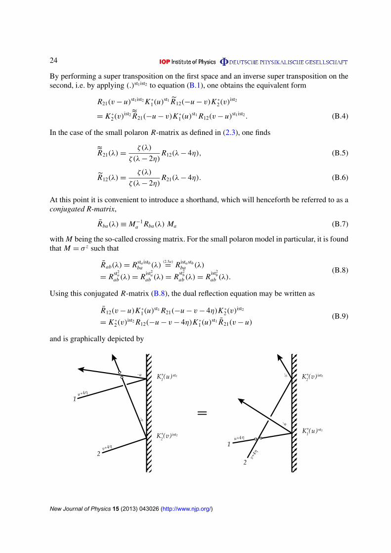
Using this conjugated R-matrix (B.8), the dual reflection equation may be written as

R12(v− u)K +1(u)

st1 R21(−u− v− 4η)K +2(v)

ist2

= K +2(v)

ist2 R12(−u− v− 4η)K +1(u)

st1 R21(v− u)(B.9)

and is graphically depicted by

K2(v) ist2+

K1(u) st1+

v+4η

-v

u+4η

-u

2

1

K2(v) ist2+

K1(u) st1+

2

1

v+4η

u+4η

-v

-u

New Journal of Physics 15 (2013) 043026 (http://www.njp.org/)

25

Appendix C. Algebraic Bethe ansatz for diagonal boundaries

The reflection equation (6.1) gives 16 fundamental commutation relations for the quantum spaceoperators A, B, C and D, of which the following three are of particular interest,

B(u)B(v)= B(v)B(u), (C.1)

A(u)B(v)=s0(u + v)s2(v− u)

s0(v− u)s2(u + v)B(v)A(u)

+ϑ(v)s2(0)

s2(u + v)B(u)

{s0(2v)s2(u + v)

ϑ(v)s0(u− v)s2(2v)A(v)− D(v)

}, (C.2)

D(u)B(v)=s4(u + v)s2(u− v)

s0(u− v)s2(u + v)B(v)D(u)−

s2(0)s4(2u)s0(2v)

ϑ(u)s2(2u)s2(u + v)s2(2v)B(u)

×

{ϑ(v)s2(2v)s2(u + v)

s0(2v)s0(u− v)D(v)−A(v)

}, (C.3)

using the abbreviation sk(λ)≡ sin(λ+ kη). To obtain the desired commutation relations, it isnecessary to make an ansatz for a shifted D-operator

D(λ)= ϑ(λ)D(λ)+φ(λ)A(λ) (C.4)

and to determine the scalar functions φ(λ) and ϑ(λ). It turns out that φ(λ)= s2(0)s2(2λ)

while ϑ(λ)remains arbitrary. Starting from the general boundary matrices given in (6.3), the diagonal casecan easily be obtained by setting α± = β± = 0. This leads to Bethe equations(

s2(ν j)

s0(ν j)

)2N

=s2(ν j −ψ+)s2(ν j −ψ−)

s0(ν j +ψ+)s0(ν j +ψ−)

M∏`=1` 6= j

s4(ν j + ν`)s2(ν j − ν`)

s0(ν j + ν`)s−2(ν j − ν`)(C.5)

and super transfer matrix eigenvalues7

3(u)= K−α(u)

(K+α(u)−

s2(0)

s2(2u)K+δ(u)

)(s2(u)

s2(−u)

)N M∏`=1

s0(u + ν`)s2(ν`− u)

s0(ν`− u)s2(u + ν`)

−K+δ(u)

(K−δ (u)−

s2(0)

s2(2u)K−α(u)

)(s2

0(u)

s2(u)s2(−u)

)N M∏`=1

s4(u + ν`)s2(u− ν`)

s0(u− ν`)s2(u + ν`). (C.6)

Here K±α,δ(u) label the diagonal entries of the boundary matrices (6.3),

K−α(u)= ω− sin(ψ− + u), K+

α(u)= ω+ sin(u + 2η +ψ+),

K−δ (u)= ω− sin(ψ−− u), K+

δ(u)= ω+ sin(u + 2η−ψ+).

(C.7)

7 Note that this result corresponds to the one obtained by Umeno et al [13]. However, the authors of [13] seem tohave made a slight mistake when substituting their formula (57) into (61) to obtain (62), which should correctlyread

t (u)= +sin(2u + 4η) sin(u + t+)

sin(2u + 2η)A(u)−

sin(u + 2η− t+)

sin(2u + 2η)D(u).

New Journal of Physics 15 (2013) 043026 (http://www.njp.org/)

26

Introducing the functions

q(u)≡M∏`=1

sin(u + 2η + ν`) sin(u− ν`), (C.8)

the eigenvalues (C.6) can be recast as

3(u)q(u)=K−α(u)

(K+α(u)−

s2(0)

s2(2u)K+δ(u)

)(s2

2(u)

s2(u)s2(−u)

)N

q(u− 2η)

−K+δ(u)

(K−δ (u)−

s2(0)

s2(2u)K−α(u)

)(s2

0(u)

s2(u)s2(−u)

)N

q(u + 2η) .

(C.9)

Appendix D. Super quantum determinants

Consider a generic B F F B graded R-matrix of the shape

R(u)=

a(u + 2η) 0 0 0

0 a(u) a(2η) 00 a(2η) a(u) 00 0 0 −a(u + 2η)

, (D.1)

where a(−u)= a(u) and a(0)= 0. At u =−2η such an R-matrix gives rise to a projector P−

onto a one-dimensional subspace

P− =−1

2a(2η)R(−2η)=

0 0 0 00 1/2 −1/2 00 −1/2 1/2 00 0 0 0

. (D.2)

Let T (u) be a representation of the graded YBA

R12(u− v) T1(u) T2(v)= T2(v) T1(u) R12(u− v) (D.3)

with the usual embeddings T1(u)≡ T (u)⊗s 1 and T2(v)≡ 1⊗s T (v), where

T (u)≡

(T 1

1 (u) T 12 (u)

T 21 (u) T 2

2 (u)

)B F

≡

(A(u) B(u)C(u) D(u)

)B F

. (D.4)

The PBC SQD is defined as

δ {T (u)} ≡ str12

{P−12T1(u) T2(u + 2η)

}(D.5)

=1

2{C(u)B(u + 2η)− A(u)D(u + 2η)

− B(u)C(u + 2η)− D(u)A(u + 2η)}. (D.6)

At v = u + 2η and after dividing by a(2η), the graded YBA yields the commutation relations

C(u)B(u + 2η)− A(u)D(u + 2η)= C(u + 2η)B(u)− D(u + 2η)A(u), (D.7)

D(u)A(u + 2η)+ B(u)C(u + 2η)= D(u + 2η)A(u)−C(u + 2η)B(u), (D.8)

B(u)C(u + 2η)+ D(u)A(u + 2η)= B(u + 2η)C(u)+ A(u + 2η)D(u). (D.9)

New Journal of Physics 15 (2013) 043026 (http://www.njp.org/)

27

These relations can be used to simplify the SQD to

δ {T (u)} = −[A(u)D(u + 2η)−C(u)B(u + 2η)]. (D.10)

It remains to show that the SQD is a central element of the graded YBA, i.e. that itsupercommutes with all the other elements A(v), B(v), C(v) and D(v) for arbitrary v. Considerthe expression

R12(u− v)R13(u−w)R23(v−w)T1(u)T2(v)T3(w). (D.11)

Employing the graded YBE once, it is obvious that

(D.11)= R23(v−w)R13(u−w) [R12(u− v)T1(u)T2(v)] T3(w) (D.12)

v→ u + 2η ⇒−2a(2η)R23(u−w + 2η)R13(u−w)P−

12T1(u)T2(u + 2η)T3(w). (D.13)

On the other hand, by applying the graded YBA relation twice, it is found that

(D.11)= T3(w) [R12(u− v)T1(u)T2(v)] R13(u−w)R23(v−w) (D.14)

v→ u + 2η ⇒−2a(2η)T3(w)P−

12T1(u)T2(u + 2η)R13(u−w)R23(u−w + 2η). (D.15)

Equating (D.13) and (D.15) and multiplying from both sides with P−12 gives

{P−12 R23(u−w + 2η)R13(u−w)P−

12}{P−

12T1(u)T2(u + 2η)P−12}T3(w)

= T3(w){P−

12T1(u)T2(u + 2η)P−12}{P−

12 R13(u−w)R23(u−w + 2η)P−12},(D.16)

where additional P−12 projectors have been inserted by virtue of the appropriate triangularityconditions. After a change of basis to the P−12 eigenbasis via A12 as defined in (3.14), it is easyto check that application of the supertrace str12{ . } yields

σ z3 δ {T (u)} T3(w)= T3(w) σ

z3 δ {T (u)} (D.17)

⇔[σ z

3 δ {T (u)} , T3(w)]= 0 (D.18)

⇔[δ {T (u)} , T i

j (w)]±= 0. (D.19)

Similarly one may introduce the object

δ{T (u)} ≡ str12{P−

12T2(u) T1(u + 2η)} (D.20)

which obeys the exact same super commutation relations and by (6.9) turns out to beproportional to the inverse of the above SQD. In particular for the considered N -site smallpolaron model, it is found that

δ(u)≡ δ {T (u)} = −ζ N (u + 2η)N∏

i=1

(−σ zqi), (D.21a)

δ(u)≡ δ{T (u)} = −1

ζ N (u)

N∏i=1

(−σ zqi), (D.21b)

where qi labels the i th quantum subspace (see section 5.2). Moreover, the commutationrelation (D.18) extends to the fused quantities according to[

σ z�n� δ {T (u)} , T

�1...n�(w)]= 0 (D.22)

with σ z�n� being defined in equation (3.16).

New Journal of Physics 15 (2013) 043026 (http://www.njp.org/)

28

In the open boundary case, the place of δ{T (u)} is taken by another object 1(u) whichwill most appropriately be called the OBC SQD. Generally, the SQD is what you get when youalter the first fusion step such that, instead of creating a higher dimensional transfer matrix byprojection on a three-dimensional auxiliary space, you now create a lower dimensional objectby projecting onto the complementary one-dimensional space. In a sense, loosely speaking, youdo a reduction instead of a fusion and find that the open boundary SQD factors as follows,

1(u)≡ str12{P12K +2(u + 2η)R12(−2u− 6η)K +

1(u)T−

1 (u)R12(2u + 2η)T −2 (u + 2η)}

= δ {K +(u)} · δ {T (u)} · δ {K −(u)} · δ{T (u)}

=

(ζ(u + 2η)

ζ(u)

)N

δ {K +(u)} · δ {K −(u)} , (D.23)

where T −(u) was defined in (6.8) and

δ {K +(u)} ≡ str12{P−

12 K +2(u + 2η) R12(−2u− 3 · 2η) K +

1(u)}

= g(−2u− 6η) · det {K +(u)} , (D.24a)

δ {K −(u)} ≡ str12{P−

12 K −

1 (u) R21(2u + 2η) K −

2 (u + 2η)}

= g(2u + 2η) · det {K −(u + 2η)} (D.24b)

with the function g(u) being introduced in the context of (2.5d). Since α± ·β± = 0, as mentionedin section 6.1, the determinants det{K ±(u)} depend only on the diagonal boundary parametersψ±. This is different from the open XXZ chain, where two parameters for each boundary enterthe expression for the quantum determinant.

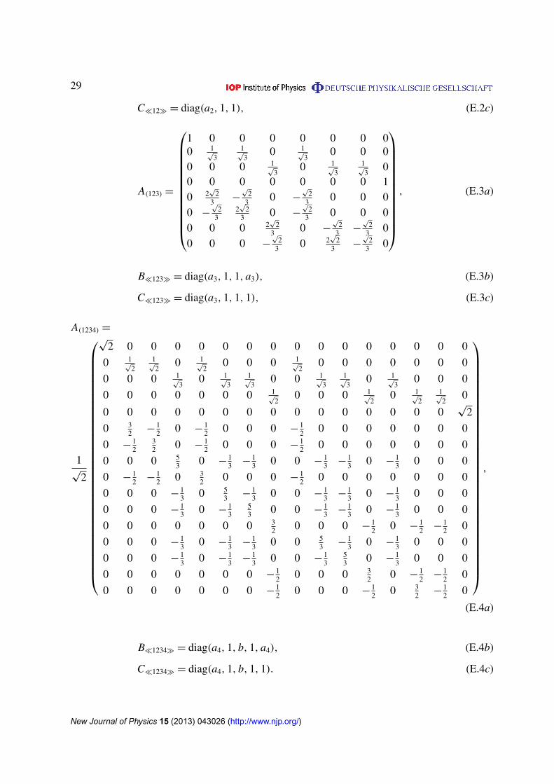
Appendix E. Transformation matrices

This appendix presents a collection of matrix representations of the various similaritytransformations employed in this paper. It is convenient to define the coefficients

an ≡

√2n

n + 1

([n]q |η=ηn

)−1/2and b =

([2]q |η=η2

[3]q |η=η3

)−1/2

, (E.1a)

where [n]q denotes the usual q-deformation of an integer n ∈ N defined by

[n]q ≡qn− q−n

q − q−1with q ≡ e2iη, (E.1b)

and to set

A(1) ≡ B�1� ≡ C�1� ≡

(1 00 1

), (E.1c)

A(12) =

1 0 0 00 1√

21√

20

0 0 0 10 1√

2−

1√

20

, (E.2a)

B�12� = diag(a2, 1, a2) (E.2b)

New Journal of Physics 15 (2013) 043026 (http://www.njp.org/)

29

C�12� = diag(a2, 1, 1), (E.2c)

A(123) =

1 0 0 0 0 0 0 00 1

√3

1√

30 1

√3

0 0 00 0 0 1

√3

0 1√

31√

30

0 0 0 0 0 0 0 10 2

√2

3 −

√2

3 0 −

√2

3 0 0 00 −

√2

32√

23 0 −

√2

3 0 0 00 0 0 2

√2

3 0 −

√2

3 −

√2

3 00 0 0 −

√2

3 0 2√

23 −

√2

3 0

, (E.3a)

B�123� = diag(a3, 1, 1, a3), (E.3b)

C�123� = diag(a3, 1, 1, 1), (E.3c)

A(1234) =

1√

2

√2 0 0 0 0 0 0 0 0 0 0 0 0 0 0 0

0 1√

21√

20 1

√2

0 0 0 1√

20 0 0 0 0 0 0

0 0 0 1√

30 1

√3

1√

30 0 1

√3

1√

30 1

√3

0 0 0

0 0 0 0 0 0 0 1√

20 0 0 1

√2

0 1√

21√

20

0 0 0 0 0 0 0 0 0 0 0 0 0 0 0√

2

0 32 −

12 0 −

12 0 0 0 −

12 0 0 0 0 0 0 0

0 −12

32 0 −

12 0 0 0 −

12 0 0 0 0 0 0 0

0 0 0 53 0 −

13 −

13 0 0 −

13 −

13 0 −

13 0 0 0

0 −12 −

12 0 3

2 0 0 0 −12 0 0 0 0 0 0 0

0 0 0 −13 0 5

3 −13 0 0 −

13 −

13 0 −

13 0 0 0

0 0 0 −13 0 −

13

53 0 0 −

13 −

13 0 −

13 0 0 0

0 0 0 0 0 0 0 32 0 0 0 −

12 0 −

12 −

12 0

0 0 0 −13 0 −

13 −

13 0 0 5

3 −13 0 −

13 0 0 0

0 0 0 −13 0 −

13 −

13 0 0 −

13

53 0 −

13 0 0 0

0 0 0 0 0 0 0 −12 0 0 0 3

2 0 −12 −

12 0

0 0 0 0 0 0 0 −12 0 0 0 −

12 0 3

2 −12 0

,

(E.4a)

B�1234� = diag(a4, 1, b, 1, a4), (E.4b)

C�1234� = diag(a4, 1, b, 1, 1). (E.4c)

New Journal of Physics 15 (2013) 043026 (http://www.njp.org/)

30

References

[1] Fedyanin V K and Yakushevich L V 1978 Teor. Mat. Fiz. 37 371–81Fedyanin V K and Yakushevich L V 1978 Theor. Math. Phys. 37 1081 (Engl. transl.)

[2] Makhankov V G and Fedyanin V K 1984 Phys. Rep. 104 1[3] Korepin V, Bolgoliubov N and GIzergin A 1993 Quantum Inverse Scattering Method and Correlation

Functions (Cambridge: Cambridge University Press)[4] Pu F-C and Zhao B-H 1986 Phys. Lett. A 118 77[5] Zhou H-Q, Jiang L-J and Wu P-F 1989 Phys. Lett. A 137 244[6] Mezincescu L and Nepomechie R I 1991 J. Phys. A: Math. Gen. 24 L17[7] Gonzalez-Ruiz A 1994 Nucl. Phys. B 424 468[8] Bracken A J, Ge X-Y, Zhang Y-Z and Zhou H-Q 1998 Nucl. Phys. B 516 588[9] Sklyanin E K 1988 J. Phys. A: Math. Gen. 21 2375

[10] Zhou H-Q 1996 Phys. J. A 29 L607[11] Zhou H-Q 1997 J. Phys. A; Math. Gen. 30 711[12] Guan X-W, Grimm U and Roemer R A 1998 Ann. Phys., Lpz. 7 518[13] Umeno Y, Fan H and Wadati M 1999 J. Phys. Soc. Japan 68 3826[14] Guan X-W, Fan H and Yang S-D 1999 Phys. Lett. A 251 79[15] Wang X-M, Fan H and Guan X-W 2000 J. Phys. Soc. Japan 69 251

Fan H and Guan X-W 1997 arXiv:cond-mat/9711150[16] Cornwell J F 1989 Group Theory in Physics (Supersymmetries and Infinite-Dimensional Algebras vol III)

(New York: Academic)[17] Nepomechie R I 2002 Nucl. Phys. B 622 615[18] Cao J, Lin H-Q, Shi K-J and Wang Y 2003 Nucl. Phys. B 663 487[19] Nepomechie R I 2004 J. Phys. A: Math. Gen. 37 433[20] Yang W-L, Nepomechie R I and Zhang Y-Z 2006 Phys. Lett. B 633 664[21] Baseilhac P and Koizumi K 2007 J. Stat. Mech. P09006 (arXiv:hep-th/0703106)[22] Galleas W 2008 Nucl. Phys. B 790 524[23] Frahm H, Seel A and Wirth T 2008 Nucl. Phys. B 802 351[24] Frahm H, Grelik J R, Seel A and Wirth T 2011 J. Phys. A: Math. Theor. 44 015001[25] Niccoli G 2012 J. Stat. Mech.P10025 (arXiv:1206.0646)[26] Grabinski A M and Frahm H 2010 J. Phys. A: Math. Theor. 43 045207[27] Yang W-L and Zhang Y-Z 2006 Nucl. Phys. B 744 312[28] Frappat L, Nepomechie R and Ragoucy E 2007 J. Stat. Mech. P09009 (arXiv:0707.0653)[29] Kulish P P, Reshetikhin N Yu and Sklyanin E K 1981 Lett. Math. Phys. 5 393[30] Mezincescu L and Nepomechie R I 1992 J. Phys. A: Math. Gen. 25 2533[31] Zhou Y 1996 Nucl. Phys. B 458 504[32] de Vega H J and Gonzalez-Ruiz A 1993 J. Phys. A: Math. Gen. 26 L519[33] Murgan R and Nepomechie R I 2005 J. Stat. Mech. P05007 (arXiv:hep-th/0504124)[34] Murgan R, Nepomechie R I and Shi C 2006 J. Stat. Mech.P08006 (arXiv:hep-th/0605223)[35] Murgan R, Nepomechie R I and Shi C 2007 J. High Energy Phys. JHEP01(2007)038[36] Kulish P P and Reshetikhin N Yu 1983 J. Sov. Math. 23 2435[37] Kirillov A N and Reshetikhin Yu N 1986 J. Sov. Math. 35 2627

Kirillov A N and Reshetikhin N Yu 1985 Zap. Nauch. Sem. LOMI 145 109–33[38] Kirillov A N and Reshetikhin N Yu 1987 J. Phys. A: Math. Gen. 20 1565[39] Zamolodchikov A B and Fateev V A 1980 Sov. J. Nucl. Phys. 32 298[40] Mezincescu L, Nepomechie R I and Rittenberg V 1990 Phys. Lett. A 147 70

New Journal of Physics 15 (2013) 043026 (http://www.njp.org/)

31

[41] Maassarani Z 1995 J. Phys. A: Math. Gen. 28 1305[42] Pfannmuller M P and Frahm H 1996 Nucl. Phys. B 479 575[43] Pfannmuller M P and Frahm H 1997 J. Phys. A: Math. Gen. 30 L543[44] Frahm H 1999 Nucl. Phys. B 559 613[45] Gruneberg J 2000 Nucl. Phys. B 568 594[46] Gohmann F and Murakami S 1998 J. Phys. A: Math. Gen. 31 7729

New Journal of Physics 15 (2013) 043026 (http://www.njp.org/)