Turbulent Flow Field Measurements of Separate Flow Round ... · baseline configuration turbulence profile indicates an asymmetric flow field, despite careful ... The JES is mounted

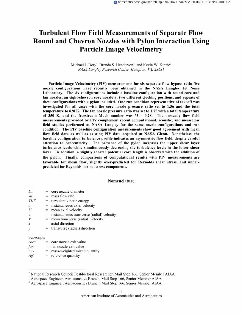
American Institute of Aeronautics and Astronautics

1

Turbulent Flow Field Measurements of Separate Flow Round and Chevron Nozzles with Pylon Interaction Using

Particle Image Velocimetry

Michael J. Doty*, Brenda S. Henderson†, and Kevin W. Kinzie‡ NASA Langley Research Center, Hampton, VA, 23681

Particle Image Velocimetry (PIV) measurements for six separate flow bypass ratio five nozzle configurations have recently been obtained in the NASA Langley Jet Noise Laboratory. The six configurations include a baseline configuration with round core and fan nozzles, an eight-chevron core nozzle at two different clocking positions, and repeats of these configurations with a pylon included. One run condition representative of takeoff was investigated for all cases with the core nozzle pressure ratio set to 1.56 and the total temperature to 828 K. The fan nozzle pressure ratio was set to 1.75 with a total temperature of 350 K, and the freestream Mach number was M = 0.28. The unsteady flow field measurements provided by PIV complement recent computational, acoustic, and mean flow field studies performed at NASA Langley for the same nozzle configurations and run condition. The PIV baseline configuration measurements show good agreement with mean flow field data as well as existing PIV data acquired at NASA Glenn. Nonetheless, the baseline configuration turbulence profile indicates an asymmetric flow field, despite careful attention to concentricity. The presence of the pylon increases the upper shear layer turbulence levels while simultaneously decreasing the turbulence levels in the lower shear layer. In addition, a slightly shorter potential core length is observed with the addition of the pylon. Finally, comparisons of computational results with PIV measurements are favorable for mean flow, slightly over-predicted for Reynolds shear stress, and under-predicted for Reynolds normal stress components.

Nomenclature Dc = core nozzle diameter m� = mass flow rate TKE = turbulent kinetic energy u = instantaneous axial velocity U = mean axial velocity v = instantaneous transverse (radial) velocity V = mean transverse (radial) velocity x = axial direction y = transverse (radial) direction Subscripts core = core nozzle exit value fan = fan nozzle exit value mix = mass-weighted mixed quantity ref = reference quantity

* National Research Council Postdoctoral Researcher, Mail Stop 166, Senior Member AIAA. † Aerospace Engineer, Aeroacoustics Branch, Mail Stop 166, Senior Member AIAA. ‡ Aerospace Engineer, Aeroacoustics Branch, Mail Stop 166, Senior Member AIAA.

https://ntrs.nasa.gov/search.jsp?R=20040074459 2020-06-05T13:09:36+00:00Z


2

I. Introduction

s aircraft noise standards become more stringent around the world, there has been an ongoing interest in aircraft noise reduction. Jet noise is a major contributor to overall aircraft noise, particularly at takeoff, and has

been an important focus for noise reduction. The evolution of more efficient higher bypass ratio (BPR) engines over the last few decades has serendipitously had the added benefit of jet noise reduction. However, obtaining further jet noise reductions with current engine technology and without penalty in weight and/or thrust will require novel approaches. One approach that is receiving increasing attention as a possible path toward further noise reduction is the investigation of installation effects. Installation effects refer to the effects on the radiated aircraft noise that are directly attributable to the installation of the propulsion system on the airframe. For jet noise, this predominantly includes pylon interaction effects with the jet flow, wing downwash-jet interaction effects, and flap-jet interactions. Furthermore, it is important to understand how these effects couple with existing noise reduction technologies such as chevron nozzles in order to optimize noise reduction at the system level. With increasingly challenging noise reduction goals, consideration of system level aeroacoustics is imperative. In order to better understand the aerodynamics and acoustics associated with installed jet engines (a discipline referred to as Propulsion-Airframe Aeroacoustics or PAA), in-depth analytical and computational studies, as well as flow field and acoustic measurements, are needed. Recent efforts at NASA have been focused on acquiring these data and developing tools for one specific installation effect – the pylon-jet plume interaction in separate flow nozzles including the effect on chevron noise reduction technology. An initial Reynolds-averaged Navier-Stokes (RANS) computational fluid dynamics (CFD) study reported by Thomas et al.1 predicted mean and turbulent flow fields for various separate flow nozzle configurations including the pylon and core chevron nozzle. More recently, Massey et al.2 improved the computations by accounting for increased mixing due to high temperature gradients and showed excellent agreement with mean flow field measurements. These results have been used by Hunter et al.3 to predict the jet noise associated with these nozzle configurations using a 3-D noise prediction code called Jet3D. Noise predictions agreed well with acoustic measurements in the forward arc and sideline locations but not in the jet aft arc. The computational predictions described previously have relied heavily on the mean flow measurements, and the jet noise predictions have relied on the computations for input and acoustic measurements for validation. Thus far, however, there have been no turbulent flow field measurements in this study to weigh against the CFD or couple with the acoustics. The current work addresses this need. Particle Image Velocimetry (PIV) is used to measure both mean and fluctuating velocity in a plane along the jet centerline for the separate flow nozzle configurations previously studied. The primary objectives of this work are to measure and evaluate the turbulent flow field of each nozzle configuration and to compare to existing CFD solutions. Efforts to apply these results more directly to acoustic predictions are discussed in Farassat et al.4 and will be the focus of future work.

II. Experimental Procedures

A. Facility Description All experiments described in this work took place in the NASA Langley Jet Noise Lab (JNL) Low Speed

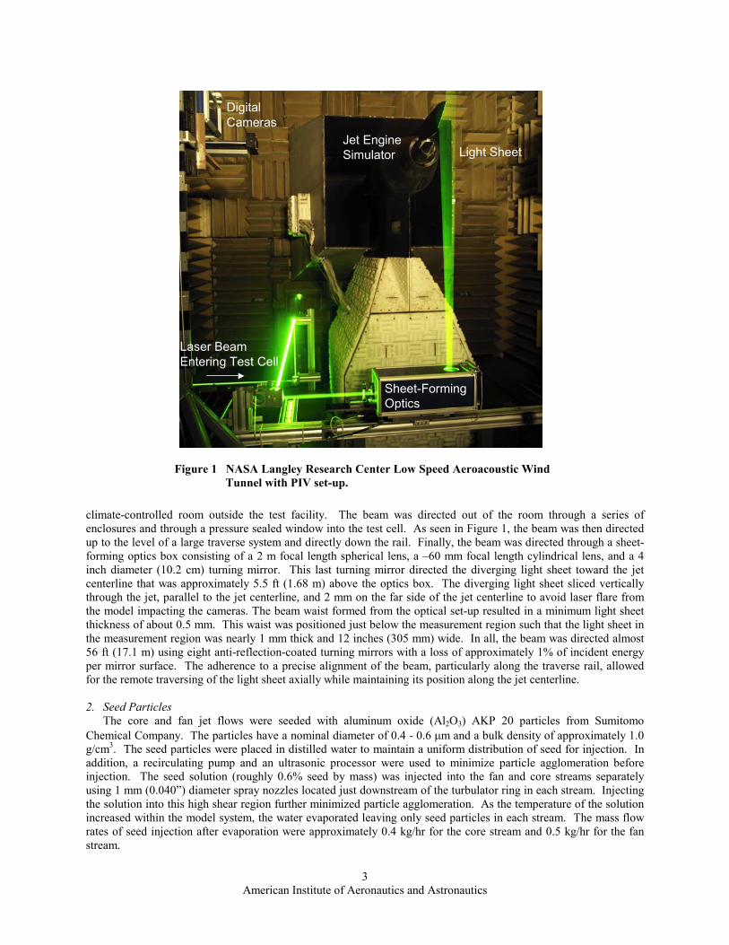
Aeroacoustic Wind Tunnel (LSAWT), shown in Figure 1. The jet engine simulator (JES) offers dual stream propulsion simulation using two independently controlled air streams and propane burners. The JES is mounted in an aeroacoustic wind tunnel capable of flows up to M = 0.32, thus producing a realistic forward-flight effect around the engine exhaust.

B. PIV System PIV is a measurement technique consisting of a double-pulsed laser light sheet illuminating seed particles in a

flow field of interest, in this case along the jet centerline as shown in Figure 1. Individual particles are tracked by cross-correlating two successive images, usually obtained with a digital camera, within a very short period of time (microseconds). The measured result is a two-component instantaneous velocity field. Correlated image pairs can then be ensemble-averaged to produce mean flow field and turbulent statistics. The major components of the PIV system used in this work are now described in more detail. 1. Laser

A dual head Nd/YAG Spectra-Physics laser generating 375 mJ/pulse and emitting 532-nm wavelength green light was used to illuminate the flow field. To avoid vibrations and thermal gradients, the laser was kept in a

A


3

climate-controlled room outside the test facility. The beam was directed out of the room through a series of enclosures and through a pressure sealed window into the test cell. As seen in Figure 1, the beam was then directed up to the level of a large traverse system and directly down the rail. Finally, the beam was directed through a sheet-forming optics box consisting of a 2 m focal length spherical lens, a –60 mm focal length cylindrical lens, and a 4 inch diameter (10.2 cm) turning mirror. This last turning mirror directed the diverging light sheet toward the jet centerline that was approximately 5.5 ft (1.68 m) above the optics box. The diverging light sheet sliced vertically through the jet, parallel to the jet centerline, and 2 mm on the far side of the jet centerline to avoid laser flare from the model impacting the cameras. The beam waist formed from the optical set-up resulted in a minimum light sheet thickness of about 0.5 mm. This waist was positioned just below the measurement region such that the light sheet in the measurement region was nearly 1 mm thick and 12 inches (305 mm) wide. In all, the beam was directed almost 56 ft (17.1 m) using eight anti-reflection-coated turning mirrors with a loss of approximately 1% of incident energy per mirror surface. The adherence to a precise alignment of the beam, particularly along the traverse rail, allowed for the remote traversing of the light sheet axially while maintaining its position along the jet centerline.

2. Seed Particles

The core and fan jet flows were seeded with aluminum oxide (Al2O3) AKP 20 particles from Sumitomo Chemical Company. The particles have a nominal diameter of 0.4 - 0.6 �m and a bulk density of approximately 1.0 g/cm3. The seed particles were placed in distilled water to maintain a uniform distribution of seed for injection. In addition, a recirculating pump and an ultrasonic processor were used to minimize particle agglomeration before injection. The seed solution (roughly 0.6% seed by mass) was injected into the fan and core streams separately using 1 mm (0.040”) diameter spray nozzles located just downstream of the turbulator ring in each stream. Injecting the solution into this high shear region further minimized particle agglomeration. As the temperature of the solution increased within the model system, the water evaporated leaving only seed particles in each stream. The mass flow rates of seed injection after evaporation were approximately 0.4 kg/hr for the core stream and 0.5 kg/hr for the fan stream.

Jet Engine Simulator

Laser Beam Entering Test Cell

Light Sheet

Sheet-Forming Optics

Digital Cameras

Jet Engine Simulator

Laser Beam Entering Test Cell

Light Sheet

Sheet-Forming Optics

Digital Cameras

Figure 1 NASA Langley Research Center Low Speed Aeroacoustic Wind Tunnel with PIV set-up.


4

The freestream wind tunnel flow was seeded with two commercial foggers – an F-100 Performance Smoke Generator from High End Systems and an MDG Max 3000 Fog Generator from MDG Fog Generators, Ltd. The MDG fogger generated 0.5 �m particles in a continuous fog volume output of approximately 85 m3/min and was placed in the settling chamber of the wind tunnel near the jet centerline. The F-100 smoke generator had an intermittent output and was placed behind the Jet Engine Simulator (JES) to direct smoke through the strut upstream of the model system when measuring the lower half of the jet plume. When measuring the upper half of the jet plume, the F-100 smoke generator was placed above the MDG fog generator in the wind tunnel settling chamber.

3. Cameras

Two Kodak ES 1.0 1008 � 1018 pixel cameras were used in a side-by-side horizontal configuration in conjunction with two Nikkor 70 mm – 300 mm zoom lenses (f/5.6) to image the flow field. While only one camera was necessary for this PIV configuration, the second camera allowed the acquisition time to be cut in half. The cameras were secured in a box on one of the two large traverse platforms approximately 58.5 inches (1.49 m) from the laser light sheet as shown in Figure 1. Within the camera box, a picomotor system was attached to each lens to permit remote focus capability. A backdrop of black velvet was attached to the other traverse platform opposite the cameras. This uniform backdrop provided a consistent and minimal background intensity level for PIV processing. The lens of each camera was adjusted to provide a field of view of approximately 5.25 inches (13.34 cm) square. Note that this field of view incorporated the addition of an in-house mask over the edges of the CCD array for added protection against laser flare. The mask reduced the field of view by roughly 0.25 inches (0.64 cm) in each direction. Accounting for an overlap of one inch between the two images, yielded a composite view of 9.75 inches wide by 5.25 inches high (24.77 cm � 13.34 cm). This composite field of view was used for all configurations except the high-resolution baseline configuration test in which the field of view for each camera was approximately 2.4 inches (6.1 cm) square. 4. Data Acquisition, Processing, and Storage

The laser and cameras were properly synchronized for image acquisition using a National Instruments NI-6602 Timer Board with a BNC 2121 Terminal Block interface. Two EPIX PIXCI-D framegrabber boards were used for image acquisition on a Dell Precision 650 Workstation with two gigabytes (GB) of RAM and an Intel Xeon 2.4 GHz processor. In conjunction with this hardware, PIVACQ5, a NASA-developed PIV acquisition software program, was used for acquisition. The laser repetition rate was 15 Hz, and the inter-frame time between laser pulses, i.e., the time separation between the two images of the pair, was typically 3.5 to 4.5 �sec. The inter-frame time was adjusted according to the expected velocities of the jet within the image area to minimize out-of-plane motion of particles and maximize accuracy of velocity measurements.

A second NASA-developed code, PIVPROC6, was used to process the PIV images. The PIVPROC code used cross-correlation processing of image pairs to generate high-quality instantaneous velocity vector maps. The multi-pass correlation option was used which allowed the initial 64 � 64 pixel subregion size to be reduced to a 32 � 32 pixel subregion size with physical dimensions of approximately 4.4 mm square. The overlap between subregions was set at 50%, corresponding to 32 pixels for the initial pass and 16 pixels for the multi-pass. A sufficient number image pairs were then acquired to obtain reasonable turbulence statistics. Initially, 800 image pairs were acquired at each measurement location, but further investigation into the convergence of the turbulence statistics revealed that 400 image pairs were sufficient. Thus, the majority of the test was conducted using 400 image pairs.

The massive amount of raw data (over 600 gigabytes) acquired during this test dictated efficient data handling procedures. A set of eight 80 GB IBM Deskstar removable hard drives were used throughout the test allowing for easy exchange of storage media between experiments. Furthermore, multiple computers could then be employed for overnight processing of data. Ultimately, the raw PIV image pairs were backed-up to Digital Linear Tape, and the processed data were stored on DVD.

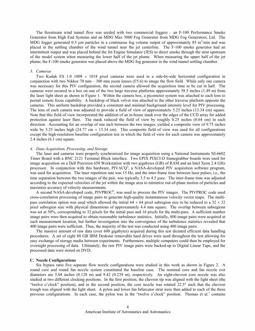
C. Nozzle Configurations Six bypass ratio five separate flow nozzle configurations were studied in this work as shown in Figure 2. A

round core and round fan nozzle system constituted the baseline case. The nominal core and fan nozzle exit diameters are 5.04 inches (0.128 m) and 9.42 (0.239 m), respectively. An eight-chevron core nozzle was also studied at two different clocking positions. In the first position, the chevron tip was aligned with the light sheet (the “twelve o’clock” position), and in the second position, the core nozzle was rotated 22.5� such that the chevron trough was aligned with the light sheet. A pylon and lower fan bifurcator strut were then added to each of the three previous configurations. In each case, the pylon was in the “twelve o’clock” position. Thomas et al.1 contains


5

further details of the chevron and pylon designs. The six configurations are summarized below with a numbering scheme consistent with previous studies1-3:

Configuration 1: Baseline round core and fan nozzles with no pylon Configuration 3: Eight chevron core nozzle (chevron tip aligned with 12 o’clock) and round fan nozzle Configuration 3R: Eight-chevron core nozzle (chevron trough aligned with 12 o’clock) and round fan nozzle Configuration 6: Baseline core and fan nozzles with pylon Configuration 4F: Eight-chevron core nozzle, round fan nozzle, and pylon (chevron tip aligned with pylon) Configuration 7: Eight-chevron core nozzle, round fan nozzle, and pylon (chevron trough aligned with pylon)

The measurements for these configurations were taken at one condition representative of the takeoff condition from a generic cycle line. The core nozzle pressure ratio was set to 1.56 with a total temperature of 828 K while the fan nozzle pressure ratio was set to 1.75 with a total temperature of 350 K. A freestream Mach number of M = 0.28 was also set. Average deviations from this operating condition were noted to be less than 0.15% for the JES operations and less than 1.0% for the wind tunnel operation. Finally, it should be noted that, because all data were taken at the same cycle point, the total thrust of the pylon configurations was roughly 6% less than that of the non-pylon configurations.

III. Experimental Results

A. System Qualification Before reporting the results of the various nozzle configurations, some metrics often used to measure the quality of PIV results will be addressed. One measure of the quality of the PIV data is the number of “good” velocity vectors that are measured at a particular location relative to the total number of image pairs that are measured. The designation of a “good” vector in this case means that the vector has met pre-determined vector acceptance criteria. It should be noted that “bad” vectors can occur from circumstances such as inadequate seeding, low levels of laser illumination, and out-of-plane particle motion. For this test, the acceptance criteria are analogous to those used by Bridges and Wernet7. Mean velocity cut-off limits of approximately � 0.35% of Ucore for both u and v are imposed,

a) Configuration 1 b) Configuration 3 c) Configuration 3R

d) Configuration 6 e) Configuration 4F f) Configuration 7

Figure 2 BPR 5 Nozzle configurations tested in the current work.


6

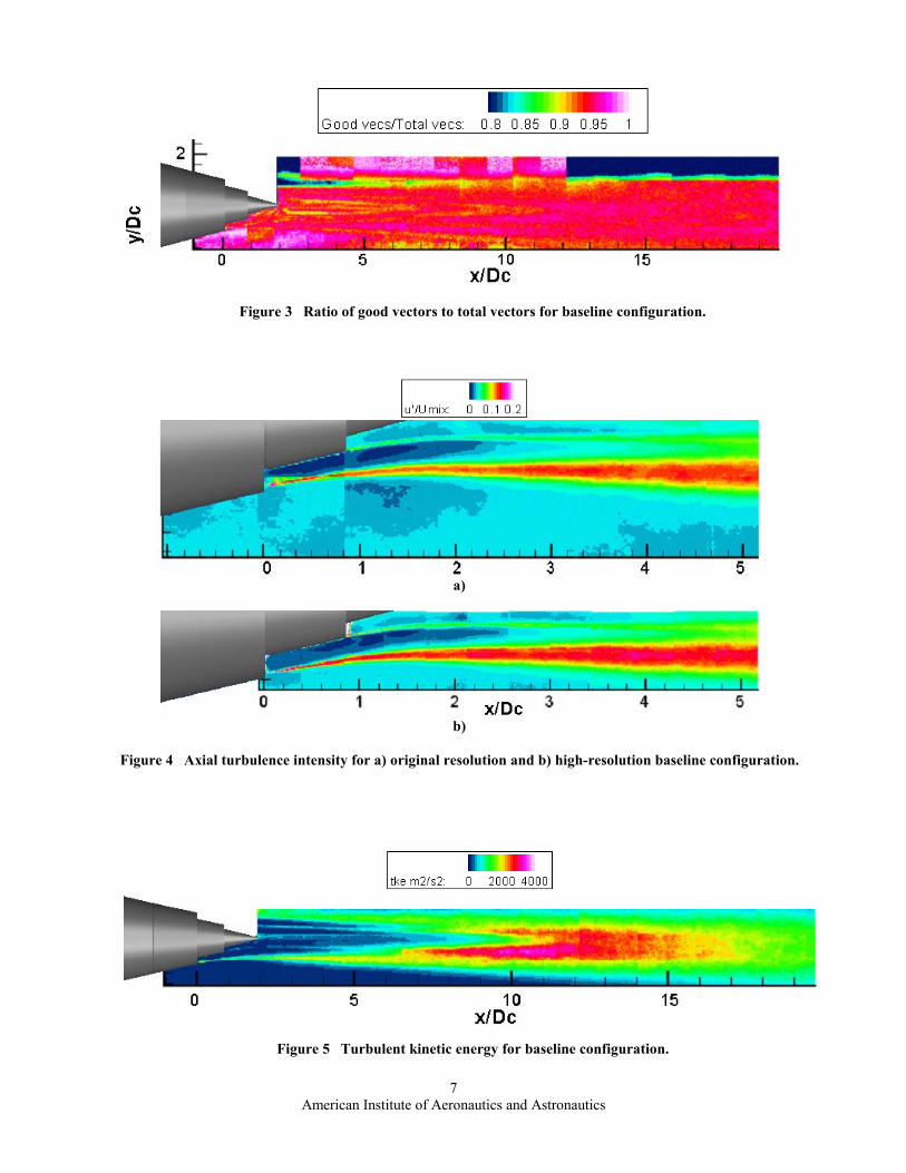
corresponding to –150 m/s to + 600 m/s for u and � 150 m/s for v. If a vector falls outside these limits, it is discarded. Furthermore, a vector is identified as an outlier and discarded if it falls outside of 2.17 standard deviations (� 3% of a standard Gaussian distribution) of the mean velocity in either u or v. The remaining vectors are considered acceptable. Figure 3 shows a contour plot of the ratio of good vectors to total vectors for Configuration 1. Both axes are non-dimensionalized by the core nozzle exit diameter; however, the zero reference is located at the fan nozzle exit because it does not experience thermal growth during testing. Note that the dark blue regions in Figure 3 indicate areas of lower quality data in which the ratio of good vectors to total vectors is less than 0.8. The lower quality data is confined to a region above the upper fan stream and is attributed to the inability to get an adequate number of fog particles into this region of the flow. The remainder of this work will not show this section of the flow field.

Spatial resolution is another significant issue to address. An important question is whether the 4.4 mm subregion size is adequate to capture the physics of the flow. By increasing the camera magnification on Configuration 1, a higher resolution experiment was conducted. Results from the high-resolution subregion size of 2.0 mm are compared to the original 4.4 mm subregion size in Figure 4. The axial component of turbulence intensity is shown in Figure 4 with u’ normalized by a mass-weighted mixed velocity as defined by:

)1(.fancore

fanfancorecoremix mm

UmUmU

��

��

�

�

�

Only in the very thin shear layers near the nozzle exit is any noticeable difference in turbulence intensity observed. As one might expect, spatial filtering of the lower resolution case results in slightly lower turbulence intensity levels in this thin shear layer region where the shear layer thickness is comparable to the subregion size. Nonetheless, the reasonable agreement further downstream in the jet justifies further experiments at the original lower resolution. Another important consideration in performing these separate flow nozzle tests is model asymmetry. It was noted that in a previous test at NASA Glenn7, a droop in the nozzle model assembly produced an asymmetric flow field. This effect was difficult to detect in the data, however, because only the lower half of the jet was examined. Furthermore, in a computational study by Birch et al.8, the turbulent flow fields of coaxial heated jets were found to be highly unstable such that even a small displacement of 1% of the core nozzle diameter resulted in a 20% asymmetry in the resulting turbulence profile. Incorporating valuable lessons from those experiments and computations convinced the current authors to examine both halves of the jet flow field for as many configurations as time would allow. Interestingly enough, in Figure 5 the contour plot of turbulent kinetic energy (TKE) for Configuration 1 also shows noticeable asymmetry. Note that TKE is approximated as

� � )2(21 222 vvuTKE ��

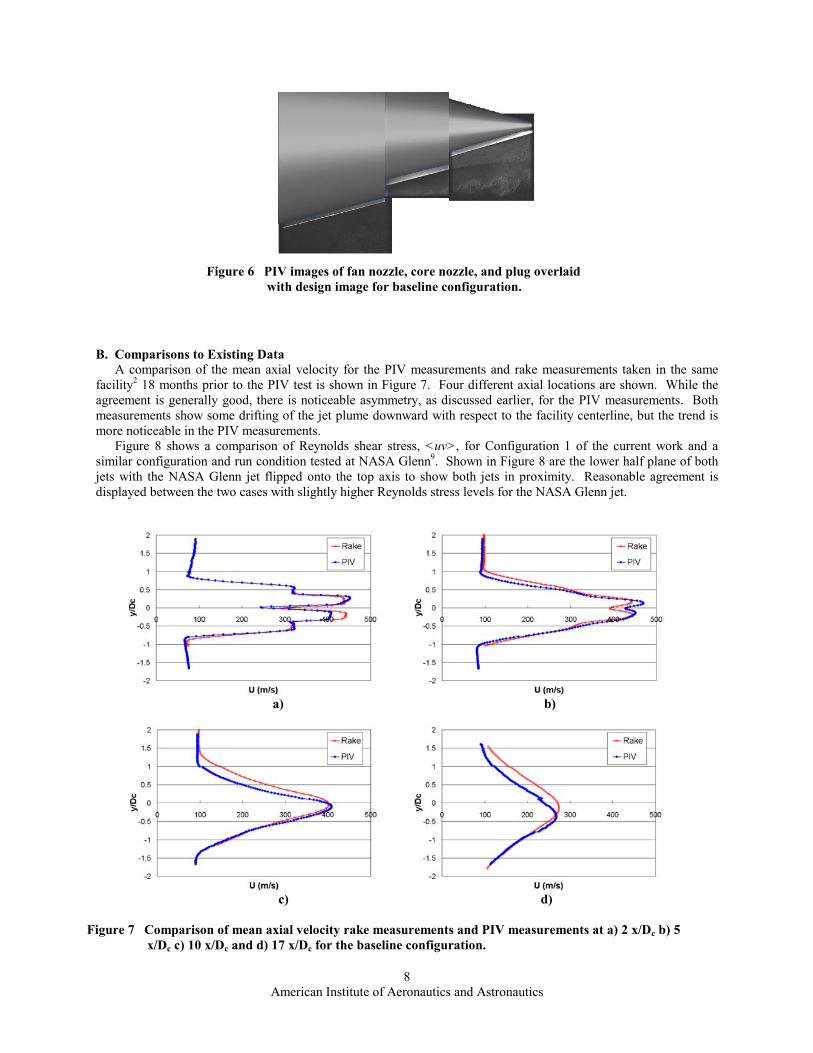
for these experiments because the third component of velocity is not attainable in the current PIV configuration. While turbulence levels are consistently higher in the lower half plane of the jet, no noticeable model droop or concentricity issues were found. Figure 6 shows an overlay of the designed model system on top of actual PIV images indicating no apparent droop in the model system. Another possible cause of the asymmetry in this test, especially when considering the mean flow measurements shown in Figure 7, is a total pressure distortion due to seed clogging the turbulence management system. Perforated sheet metal turbulence management screens showed seed accumulation upon rig disassembly that could have contributed to distortion of the total pressure in the supply flow. However, chevron configurations tested later in the experiment did not show as large of asymmetry in the mean flow or turbulence quantities as the baseline case that was tested first. This still leaves open the possibility of some type of instability in the baseline case that causes an asymmetry to develop in the flow field or a combination and interaction of these effects. These results together with work from Birch et al.8 and Bridges and Wernet7 indicate that, for numerous reasons, one should be very cautious about assuming a priori an axisymmetric flow field for heated separate flow nozzle systems in an experimental facility.


7

Figure 3 Ratio of good vectors to total vectors for baseline configuration.

a)

b)

Figure 4 Axial turbulence intensity for a) original resolution and b) high-resolution baseline configuration.

Figure 5 Turbulent kinetic energy for baseline configuration.


8

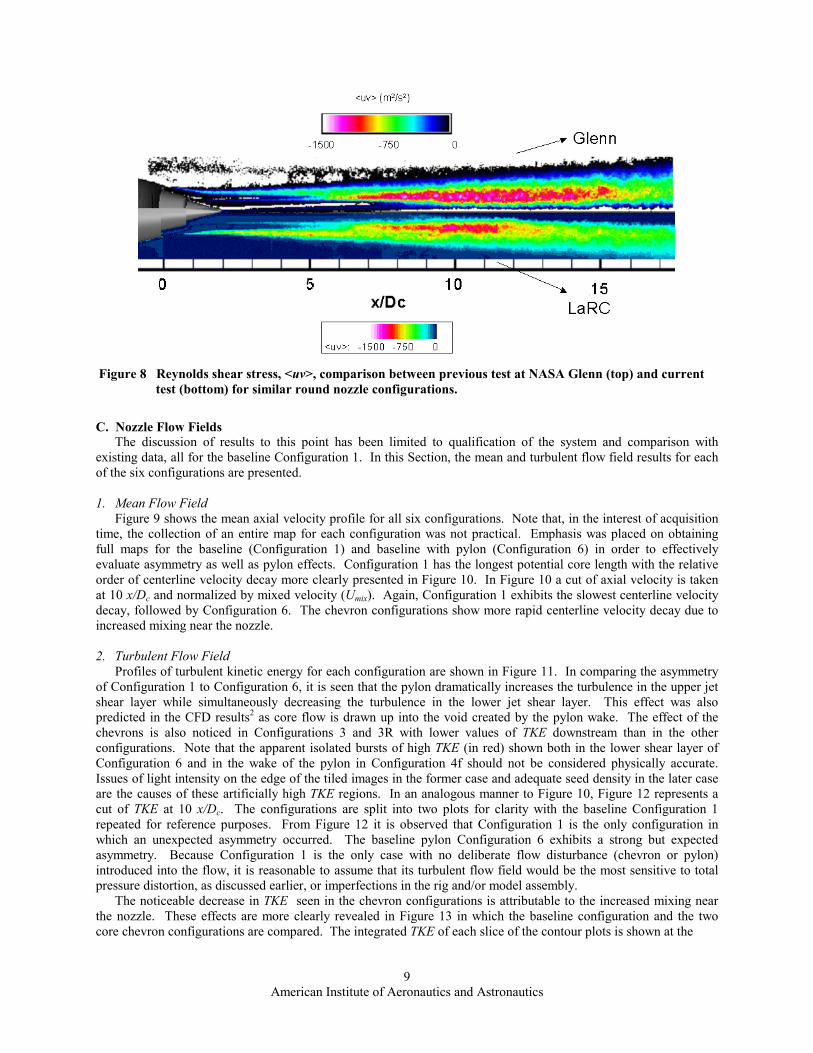
B. Comparisons to Existing Data A comparison of the mean axial velocity for the PIV measurements and rake measurements taken in the same facility2 18 months prior to the PIV test is shown in Figure 7. Four different axial locations are shown. While the agreement is generally good, there is noticeable asymmetry, as discussed earlier, for the PIV measurements. Both measurements show some drifting of the jet plume downward with respect to the facility centerline, but the trend is more noticeable in the PIV measurements. Figure 8 shows a comparison of Reynolds shear stress, <uv>, for Configuration 1 of the current work and a similar configuration and run condition tested at NASA Glenn9. Shown in Figure 8 are the lower half plane of both jets with the NASA Glenn jet flipped onto the top axis to show both jets in proximity. Reasonable agreement is displayed between the two cases with slightly higher Reynolds stress levels for the NASA Glenn jet.

Figure 6 PIV images of fan nozzle, core nozzle, and plug overlaid with design image for baseline configuration.

a) b)

c) d)

Figure 7 Comparison of mean axial velocity rake measurements and PIV measurements at a) 2 x/Dc b) 5 x/Dc c) 10 x/Dc and d) 17 x/Dc for the baseline configuration.


9

C. Nozzle Flow Fields The discussion of results to this point has been limited to qualification of the system and comparison with existing data, all for the baseline Configuration 1. In this Section, the mean and turbulent flow field results for each of the six configurations are presented.

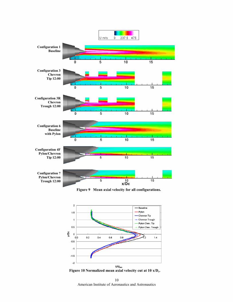
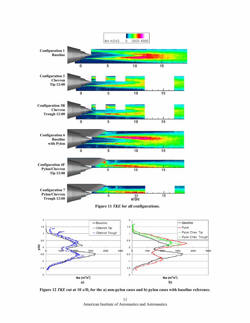
1. Mean Flow Field Figure 9 shows the mean axial velocity profile for all six configurations. Note that, in the interest of acquisition time, the collection of an entire map for each configuration was not practical. Emphasis was placed on obtaining full maps for the baseline (Configuration 1) and baseline with pylon (Configuration 6) in order to effectively evaluate asymmetry as well as pylon effects. Configuration 1 has the longest potential core length with the relative order of centerline velocity decay more clearly presented in Figure 10. In Figure 10 a cut of axial velocity is taken at 10 x/Dc and normalized by mixed velocity (Umix). Again, Configuration 1 exhibits the slowest centerline velocity decay, followed by Configuration 6. The chevron configurations show more rapid centerline velocity decay due to increased mixing near the nozzle. 2. Turbulent Flow Field Profiles of turbulent kinetic energy for each configuration are shown in Figure 11. In comparing the asymmetry of Configuration 1 to Configuration 6, it is seen that the pylon dramatically increases the turbulence in the upper jet shear layer while simultaneously decreasing the turbulence in the lower jet shear layer. This effect was also predicted in the CFD results2 as core flow is drawn up into the void created by the pylon wake. The effect of the chevrons is also noticed in Configurations 3 and 3R with lower values of TKE downstream than in the other configurations. Note that the apparent isolated bursts of high TKE (in red) shown both in the lower shear layer of Configuration 6 and in the wake of the pylon in Configuration 4f should not be considered physically accurate. Issues of light intensity on the edge of the tiled images in the former case and adequate seed density in the later case are the causes of these artificially high TKE regions. In an analogous manner to Figure 10, Figure 12 represents a cut of TKE at 10 x/Dc. The configurations are split into two plots for clarity with the baseline Configuration 1 repeated for reference purposes. From Figure 12 it is observed that Configuration 1 is the only configuration in which an unexpected asymmetry occurred. The baseline pylon Configuration 6 exhibits a strong but expected asymmetry. Because Configuration 1 is the only case with no deliberate flow disturbance (chevron or pylon) introduced into the flow, it is reasonable to assume that its turbulent flow field would be the most sensitive to total pressure distortion, as discussed earlier, or imperfections in the rig and/or model assembly. The noticeable decrease in TKE seen in the chevron configurations is attributable to the increased mixing near the nozzle. These effects are more clearly revealed in Figure 13 in which the baseline configuration and the two core chevron configurations are compared. The integrated TKE of each slice of the contour plots is shown at the

Figure 8 Reynolds shear stress, <uv>, comparison between previous test at NASA Glenn (top) and current test (bottom) for similar round nozzle configurations.


10

Figure 9 Mean axial velocity for all configurations.

Configuration 1Baseline

Configuration 3Chevron

Tip 12:00

Configuration 3RChevron

Trough 12:00

Configuration 6 Baseline

with Pylon

Configuration 4FPylon/Chevron

Tip 12:00

Configuration 7 Pylon/Chevron

Trough 12:00

Figure 10 Normalized mean axial velocity cut at 10 x/Dc.


11

Figure 11 TKE for all configurations.


Configuration 3 Chevron

Tip 12:00


Trough 12:00


with Pylon

Configuration 4FPylon/Chevron

Tip 12:00

Configuration 7 Pylon/Chevron

Trough 12:00

a) b)

Figure 12 TKE cut at 10 x/Dc for the a) non-pylon cases and b) pylon cases with baseline reference.


12

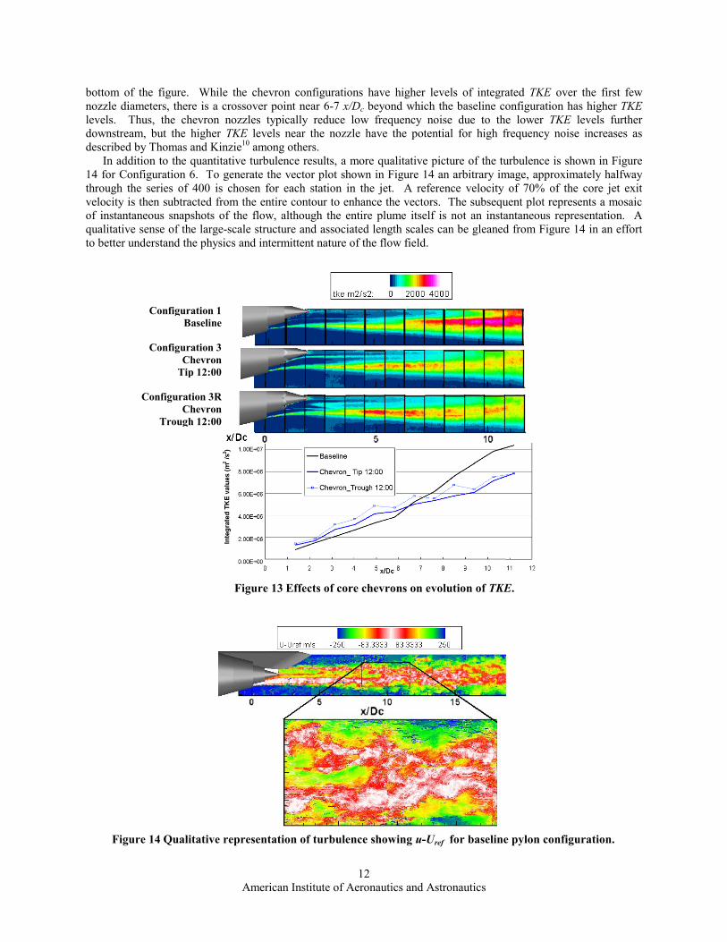
bottom of the figure. While the chevron configurations have higher levels of integrated TKE over the first few nozzle diameters, there is a crossover point near 6-7 x/Dc beyond which the baseline configuration has higher TKE levels. Thus, the chevron nozzles typically reduce low frequency noise due to the lower TKE levels further downstream, but the higher TKE levels near the nozzle have the potential for high frequency noise increases as described by Thomas and Kinzie10 among others. In addition to the quantitative turbulence results, a more qualitative picture of the turbulence is shown in Figure 14 for Configuration 6. To generate the vector plot shown in Figure 14 an arbitrary image, approximately halfway through the series of 400 is chosen for each station in the jet. A reference velocity of 70% of the core jet exit velocity is then subtracted from the entire contour to enhance the vectors. The subsequent plot represents a mosaic of instantaneous snapshots of the flow, although the entire plume itself is not an instantaneous representation. A qualitative sense of the large-scale structure and associated length scales can be gleaned from Figure 14 in an effort to better understand the physics and intermittent nature of the flow field.

Figure 13 Effects of core chevrons on evolution of TKE.


Configuration 3 Chevron

Tip 12:00


Trough 12:00

Figure 14 Qualitative representation of turbulence showing u-Uref for baseline pylon configuration.


13

D. Comparisons to CFD An essential part of a successful noise reduction program is the establishment an accurate noise prediction

methodology, which itself is heavily dependent on accurate CFD results. As these various tools evolve in the PAA program, it is important to evaluate how the CFD compares to the current experimental results. The CFD results are from Massey et al.2 using a three-dimensional Reynolds-averaged Navier-Stokes solver (PAB3D) which employs a standard two-equation k-� turbulence model with a linear algebraic Reynolds stress representation. Furthermore, a correction is applied to the eddy viscosity model that is based on total temperature gradient in order to predict more accurate levels of mixing for high temperature jets.

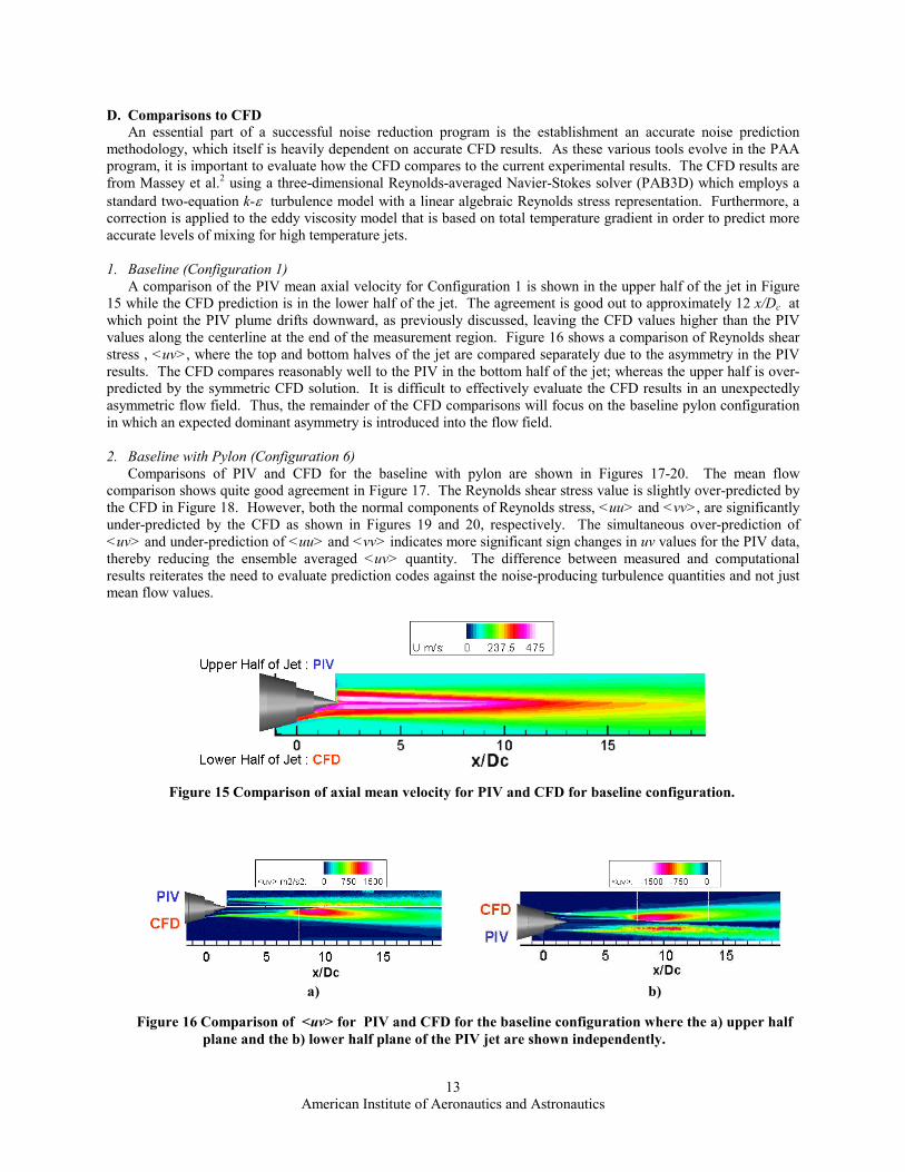
1. Baseline (Configuration 1) A comparison of the PIV mean axial velocity for Configuration 1 is shown in the upper half of the jet in Figure 15 while the CFD prediction is in the lower half of the jet. The agreement is good out to approximately 12 x/Dc at which point the PIV plume drifts downward, as previously discussed, leaving the CFD values higher than the PIV values along the centerline at the end of the measurement region. Figure 16 shows a comparison of Reynolds shear stress , <uv>, where the top and bottom halves of the jet are compared separately due to the asymmetry in the PIV results. The CFD compares reasonably well to the PIV in the bottom half of the jet; whereas the upper half is over-predicted by the symmetric CFD solution. It is difficult to effectively evaluate the CFD results in an unexpectedly asymmetric flow field. Thus, the remainder of the CFD comparisons will focus on the baseline pylon configuration in which an expected dominant asymmetry is introduced into the flow field. 2. Baseline with Pylon (Configuration 6)

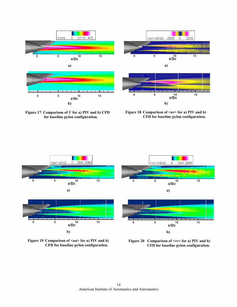
Comparisons of PIV and CFD for the baseline with pylon are shown in Figures 17-20. The mean flow comparison shows quite good agreement in Figure 17. The Reynolds shear stress value is slightly over-predicted by the CFD in Figure 18. However, both the normal components of Reynolds stress, <uu> and <vv>, are significantly under-predicted by the CFD as shown in Figures 19 and 20, respectively. The simultaneous over-prediction of <uv> and under-prediction of <uu> and <vv> indicates more significant sign changes in uv values for the PIV data, thereby reducing the ensemble averaged <uv> quantity. The difference between measured and computational results reiterates the need to evaluate prediction codes against the noise-producing turbulence quantities and not just mean flow values.

Figure 15 Comparison of axial mean velocity for PIV and CFD for baseline configuration.

a) b)

Figure 16 Comparison of <uv> for PIV and CFD for the baseline configuration where the a) upper half

plane and the b) lower half plane of the PIV jet are shown independently.


14

a)

b)

Figure 17 Comparison of U for a) PIV and b) CFD for baseline pylon configuration.

a)

b)

Figure 18 Comparison of <uv> for a) PIV and b) CFD for baseline pylon configuration.

a)

b)

Figure 19 Comparison of <uu> for a) PIV and b) CFD for baseline pylon configuration.

a)

b)

Figure 20 Comparison of <vv> for a) PIV and b) CFD for baseline pylon configuration.


15

IV. Concluding Remarks This paper presents and discusses PIV measurements of six separate flow nozzle configurations. These

turbulence measurements complement previous mean flow and acoustic measurements and flow field and noise predictions in an effort to better understand, model, and predict the noise associated with jet-pylon interactions. After presenting data qualifying the PIV measurement system, the current work demonstrates reasonable agreement with existing mean flow and PIV data of similar experiments. The asymmetry of the baseline configuration may be attributable to the sensitivity of this particular configuration to total pressure distortion or other imperfections in the rig and/or model assembly.

Mean and fluctuating flow field results show the baseline configuration to have the slowest centerline velocity decay followed by the baseline pylon case. Furthermore, with the addition of the pylon to the baseline configuration, the upper half plane of the jet shows dramatically higher turbulence levels while the lower shear layer turbulence levels decrease. The core chevron nozzle configurations, when compared to the baseline configuration, show slightly higher TKE levels near the nozzle with a benefit of significantly lower TKE levels further downstream. Comparisons of CFD results with PIV measurements show good agreement in mean flow and slight over-prediction in Reynolds shear stress, but under-prediction of Reynolds normal stress terms. Future efforts will involve applying these PIV measurements to improve flow field and noise predictions. In addition, implementation of a three-component PIV system capable of capturing cross sections of the jet plume would enhance the understanding of jet- pylon and chevron effects.

Acknowledgments The authors sincerely thank the entire Jet Noise Lab team for their efforts during this challenging test. The input

from Russ Thomas as the Propulsion Airframe Aeroacoustics manager is gratefully acknowledged, as well as the communication and support from the PAA computational team including Steve Massey and Alaa Emilgui of Eagle Aeronautics, and S. Paul Pao, K. S. Abdol-Hamid, and Craig Hunter of NASA Langley Research Center. Furthermore, the assistance of Scott Bartram and William Humphreys at NASA Langley and Mark Wernet and James Bridges at NASA Glenn during the implementation of the PIV system is gratefully acknowledged. Finally, M. J. Doty wishes to acknowledge the National Research Council for program support during this work.

References 1 Thomas, R. H., Kinzie, K. W., and Paul Pao, S., “Computational Analysis of a Pylon-Chevron Core Nozzle Interaction,” AIAA Paper 2001-2185, May 2001. 2 Massey, S. and Thomas, R., “Computational and Experimental Flowfield Analyses of Separate Flow Chevron Nozzles and Pylon Interaction,” AIAA Paper 2003-3212, May 2003. 3 Hunter, C. Pao, S. and Thomas, R., “Development of a Jet Noise Prediction Method for Installed Jet Configurations,” AIAA Paper 2003-3169, May 2003. 4 Farassat, F., Doty, M. J., and Hunter, C., “The Acoustic Analogy – A Powerful Tool in Aeroacoustics with Emphasis on Jet Noise Prediction,” AIAA Paper 2004-2872, May 2004. 5 Wernet, M. P., “PIVACQ Software Manual Version 2.2,” NASA Glenn Research Center, January 2002. 6 Wernet, M. P., “Fuzzy Logic Enhanced Digital PIV Processing Software,” NASA TM-1999-209274, 1999. 7 Bridges, J. and Wernet, M. P., “Turbulence Measurements of Separate Flow Nozzles with Mixing Enhancement Features,” AIAA Paper 2002-2484, June 2002. 8 Birch, S. F., Lyubimov, D. A., Secundov, A. N., and Yakubovsky, K. Ya., “Numerical Modeling Requirements for Coaxial and Chevron Nozzle Flows,” AIAA Paper 2003-3287, May 2003. 9 Bridges, J., “Measurements of Turbulent Flow Field in Separate Flow Nozzles with Enhanced Mixing Devices – Test Report,” NASA TM-2002-211366, 2002. 10 Thomas, R. and Kinzie K., “Jet-Pylon Interaction Effects for High Bypass Ratio Separate Flow and Chevron Nozzles,” AIAA Paper 2004-2827, May 2004.

Documents

Turbulent Flow Field Measurements of Separate Flow Round ... · baseline configuration turbulence profile indicates an asymmetric flow field, despite careful ... The JES is mounted