Two-grid covolume schemes for elliptic problems

COMMUNICATIONS IN NUMERICAL METHODS IN ENGINEERINGCommun. Numer. Meth. Engng 2006; 22:397–409Published online 6 October 2005 in Wiley InterScience (www.interscience.wiley.com). DOI: 10.1002/cnm.822

Two-grid covolume schemes for elliptic problems

Cheng Wang1, Ziping Huang2;∗;† and Likang Li3

1Department of Applied Mathematics; Tongji University; Shanghai 200092; People’s Republic of China2Chinese-German College, Tongji University, Shanghai 200092, People’s Republic of China

3Department of Mathematics; Fudan University; Shanghai 200433; People’s Republic of China

SUMMARY

In this paper, we present and analyse some local and parallel covolume algorithms for second-orderelliptic problems. We �rst prove some local a priori error estimates for covolume method. With theseresults, we shall apply the two-grid strategy to covolume approximation to give two novel covolumealgorithms, and show that the convergence rates of these algorithms are optimal in piecewise H 1-norm.Numerical results con�rming the theory are also provided. Copyright ? 2005 John Wiley & Sons, Ltd.

KEY WORDS: second-order elliptic problems; covolume method; two-grid discretization

1. INTRODUCTION

The covolume method is a popular discretization technique for partial di�erential equations,especially those arising from physical conservation laws including mass, momentum, and en-ergy. This is mainly due to its important property of inheriting the physical conservation lawsof the original problem locally, as well as its easier derivation of the linear algebraic system incontrast with conventional �nite element method. Recently, there has been intensive researchin covolume method for the elliptic partial di�erential equations. We refer to References [1–3]and cited references there for more details.However, most of these papers are related to the construction of discretization formula-

tion and the convergence behaviour of covolume method, while only a few are concernedwith the e�cient ways of solving algebraic systems generated by covolume method [4–6].The purpose of this paper is to present some parallel covolume algorithms for the second-order elliptic boundary value problems and give the corresponding error analyses. Thesealgorithms are based on the two-grid discretization, and therefore can be regarded as the

∗Correspondence to: Ziping Huang, Chinese-German College, Tongji University, Shanghai 200092, People’sRepublic of China.

†E-mail: [email protected]

Contract=grant sponsor: National Natural Science Foundation of China; contract=grant number: 40074031

Received 21 June 2004Revised 16 June 2005

Copyright ? 2005 John Wiley & Sons, Ltd. Accepted 22 July 2005

398 C. WANG, Z. HUANG AND L. LI

so-called two-grid method to some extent. The two-grid method was introduced by Xu [7, 8]for non-symmetric and non-linear elliptic problems. And later on, it has been further in-vestigated by many others [9–13]. The main idea is that for a solution to some ellipticproblems, low frequency components can be approximated well by a relatively coarse gridand high frequency components can be computed on a �ne grid by some local and parallelprocedures.In comparison with �nite element method, covolume method is not built upon the variational

form of the original problem, so the error analysis is more di�cult to deal with. We followthe techniques of Chou and Li and Ewing et al. [1, 14] to overcome this di�culty. The mainingredients in their approach are: (i) the introduction of a reasonable ‘dual’ �nite elementmethod related to the covolume method considered, and (ii) the conversion of the erroranalysis of the covolume method to the estimate of the deviation between the solution of thecovolume method and the solution of the induced �nite element method.With the technique mentioned above, we can prove a local a priori error estimate of

covolume method (see Lemma 3.2), which plays a crucial role in the convergence analy-sis of our parallel covolume algorithms. It is interesting to note that the estimate indicatesthere exists a local superconvergence for covolume approximation. Motivated by this obser-vation, we propose a local and parallel covolume method by applying the two-grid strategyto covolume approximation case. The error estimate for this algorithm is proved to be opti-mal in piecewise H 1-norm. Furthermore, noticing that the symmetric positive de�nite lead-ing term −�u dominates the equation on high frequencies, we take a further step to giveanother algorithm and follow the analysis framework established for the �rst algorithm toobtain the optimal error estimate. The remainder of this paper is organized as follows. InSection 2, we describe the second-order elliptic boundary value problem, and write down its�nite element and covolume discretizations, as well as the properties of these two discretiza-tions. In Section 3, we present some local and parallel covolume algorithms and give thedetailed analysis of the error estimates. Finally, in Section 4, some numerical experiments areprovided to support the theory.

2. DESCRIPTIONS OF THE DISCRETIZATION METHODS

Consider the general second-order elliptic boundary value problem

−div(A∇u+ bu) + qu=f in �

u=0 on @�(1)

where � is a plane polygonal domain with the boundary @�, b=[b1; b2]t ∈ (W 1;∞(�))2,q∈L∞(�), f∈H 1(�), and A=(aij)2×2 ∈ (W 1;∞(�))4 is a given real symmetric matrix-valuedfunction. We assume that A satis�es the following uniform ellipticity condition: there existsa positive constant c such that

c�t�6 �tA(x1; x2)�; ∀�∈R2; (x1; x2)∈ ��

Throughout this paper, we shall adopt the standard de�nitions for Sobolev spaces and theirnorms and semi-norms [15], and denote by C (or c) a generic positive constant independentof h and other relative parameters, which may stand for di�erent values in di�erent places.

Copyright ? 2005 John Wiley & Sons, Ltd. Commun. Numer. Meth. Engng 2006; 22:397–409

TWO-GRID COVOLUME SCHEMES FOR ELLIPTIC PROBLEMS 399

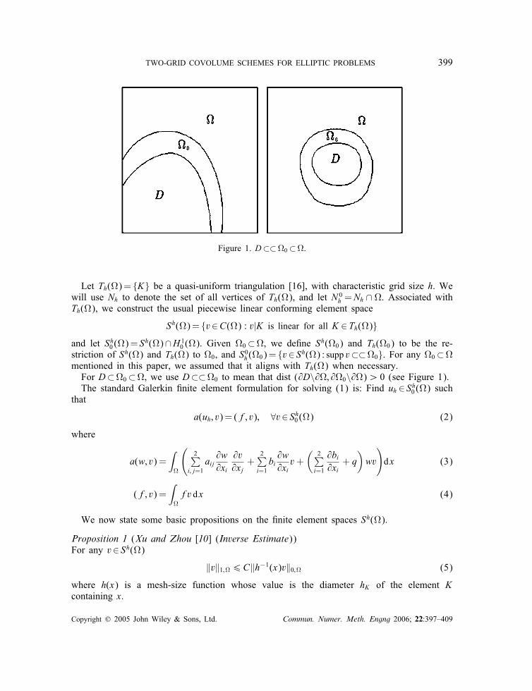
Figure 1. D⊂⊂�0 ⊂�.

Let Th(�)= {K} be a quasi-uniform triangulation [16], with characteristic grid size h. Wewill use Nh to denote the set of all vertices of Th(�), and let N 0h =Nh ∩ �. Associated withTh(�), we construct the usual piecewise linear conforming element space

Sh(�)= {v∈C(�) : v|K is linear for all K ∈Th(�)}and let Sh0 (�)= S

h(�)∩H 10 (�). Given �0 ⊂�, we de�ne Sh(�0) and Th(�0) to be the re-

striction of Sh(�) and Th(�) to �0, and S0h (�0)= {v∈ Sh(�) : supp v⊂⊂�0}. For any �0 ⊂�mentioned in this paper, we assumed that it aligns with Th(�) when necessary.For D⊂�0 ⊂�, we use D⊂⊂�0 to mean that dist (@D\@�; @�0\@�)¿ 0 (see Figure 1).The standard Galerkin �nite element formulation for solving (1) is: Find uh ∈ Sh0 (�) such

that

a(uh; v)= (f; v); ∀v∈ Sh0 (�) (2)

where

a(w; v) =∫�

(2∑

i; j=1aij@w@xi

@v@xj

+2∑i=1bi@w@xiv+

(2∑i=1

@bi@xi

+ q)wv

)dx (3)

(f; v) =∫�fv dx (4)

We now state some basic propositions on the �nite element spaces Sh(�).

Proposition 1 (Xu and Zhou [10] (Inverse Estimate))For any v∈ Sh(�)

‖v‖1;�6C‖h−1(x)v‖0;� (5)

where h(x) is a mesh-size function whose value is the diameter hK of the element Kcontaining x.



Proposition 2 (Xu and Zhou [10]) (Superapproximation)For D⊂�0 ⊂⊂�, let !∈C∞

0 (�) with supp !⊂⊂D. Then there exists v∈ S0h (D) such that‖(!w − v)‖1; D6Ch‖w‖1; D; ∀w∈ Sh(D) (6)

For some �0 ⊂�, we need the following assumption.Assumption 1 (Xu and Zhou [10])For f∈L2(�), then there exists w∈H 1

0 (�0) satisfying

a(v; w)= (f; v); ∀v∈H 10 (�0)

and

‖w‖1+�;�06C‖f‖−1+�;�0 ; 0¡�6 1 (7)

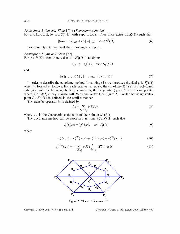
In order to describe the covolume method for solving (1), we introduce the dual grid T ∗h (�)

which is formed as follows. For each interior vertex P0, the covolume K∗(P0) is a polygonalsubregion with the boundary built by connecting the barycentre QK of K with its midpoints,where K ∈Th(�) is any triangle with P0 as one vertex (see Figure 2). For the boundary vertexpoint P0, K∗(P0) is de�ned in the similar manner.The transfer operator Ih is de�ned by

Ihv=∑

P0 ∈N 0hv(P0)�P0 (8)

where �P0 is the characteristic function of the volume K∗(P0).

The covolume method can be expressed as: Find u∗h ∈ Sh0 (�) such that

a∗h(u

∗h ; v)= (f; Ihv); ∀v∈ Sh0 (�) (9)

where

a∗h(w; v) = a

∗(2)h (w; v) + a∗(1)

h (w; v) + a∗(0)h (w; v) (10)

a∗(2)h (w; v) =− ∑

P0∈N 0hv(P0)

∫@K∗

P0

A∇w · n ds (11)

Q1

P1

P2

P0

M1

K*

P3 P

4

P5

P6

M2

M3 M

4

M5

M6

Q2

Q3

Q4

Q5

Q6

Figure 2. The dual element K∗.



a∗(1)h (w; v) =− ∑

P0∈N 0hv(P0)

∫@K∗

P0

bw · n ds (12)

a∗(0)h (w; v) =

∑P0∈N 0h

v(P0)∫K∗P0

qw dx (13)

We now give some estimates for the transfer operator Ih and the deviation dh(·; ·) betweenthe two bilinear forms a(·; ·) and a∗

h(·; ·), that is,dh(w; v)= a(w; v)− a∗

h(w; v); ∀w; v∈ Sh0 (�) (14)

Lemma 2.1 (Chou and Li [1])There exists a positive constant C, independent of h, such that

‖v− Ihv‖0;�6Ch‖v‖1;�; ∀v∈ Sh0 (�) (15)

|dh(u; v)|6Ch‖u‖1;�‖v‖1;�; ∀u; v∈ Sh0 (�) (16)

The H 1 and L2 error estimates of the covolume method for problem (1) are statedas follows.

Lemma 2.2 (Chou and Li [1], Ewing et al. [14])Assume that u and uh are solutions of (1) and (9), respectively, and u∈H 2(�); f∈H 1(�).Then there exists a positive constant C, independent of h, such that

‖uh − u‖1;�6Ch‖u‖2;� (17)

‖uh − u‖0;�6Ch2(‖u‖2;� + ‖f‖1;�) (18)

3. NEW LOCAL AND PARALLEL COVOLUME ALGORITHMS

In this section, we present some local and parallel covolume algorithms and give the corre-sponding error analysis.Firstly, we prove a local a priori error estimate of covolume approximation.

Lemma 3.1 (Xu and Zhou [10])Assume that �0 ⊂⊂� and !∈C∞

0 (�) such that supp!⊂⊂�0, then we have‖!w‖21;�6 2a(w;!2w) + C‖w‖20;�0 ; ∀w∈H 1

0 (�) (19)

Lemma 3.2Assume that f∈L2(�); D⊂⊂�0 ⊂⊂�, and there exists w∈ Sh(�0) satisfying

a∗h(w; v) = (f; Ihv); ∀v∈ S0h (�0) (20)

then the following estimate holds:

‖w‖1; D6 ‖w‖0;�0 + ‖f‖0;�0 (21)



ProofLet �1;�2 satisfy

D⊂⊂�2 ⊂⊂�1 ⊂⊂�0Choose D1 ⊂� satisfying D⊂⊂D1 ⊂⊂�2 and !∈C∞

0 (�) such that !≡ 1 on �D1 andsupp!⊂⊂�2. Then from Proposition 2, there exists v∈ S0h (�2) such that

‖!2w − v‖1;�26Ch‖w‖1;�2 (22)

which implies

a(w;!2w − v)6Ch‖w‖21;�2 (23)

and

|(f; v)|6C‖f‖0;�0‖v‖0;�26C‖f‖0;�0(h‖w‖1;�2 + ‖!w‖1;�2) (24)

Since v∈ S0h (�2)⊂ S0h (�0), we get

a(w;!2w) = a(w;!2w − v) + a(w; v)= a(w;!2w − v) + a(w; v)− a∗

h(w; v) + (f; Ihv)− (f; v) + (f; v)= a(w;!2w − v) + d(w; v) + (f; Ihv− v) + (f; v) (25)

Combining (15), (16), (19), (22), (23) and (24), we have

‖!w‖21;�6C(a(w;!2w) + ‖w‖20;�0)6C(h‖w‖21;�2 + ‖f‖0;�0(h‖w‖1;�2 + ‖!w‖1;�2) + ‖w‖20;�0) (26)

Then, it follows that

‖w‖1; D6C(h1=2‖w‖1;�2 + ‖w‖0;�0 + ‖f‖0;�0) (27)

A similar argument leads to

‖w‖1;�26C(h1=2‖w‖1;�0 + ‖w‖0;�0 + ‖f‖0;�0) (28)

Therefore, we get from Proposition 1 that

‖w‖1; D6C(h‖w‖1;�0 + ‖w‖0;�0 + ‖f‖0;�0)6C(h‖h−1(x)w‖0;�0 + ‖w‖0;�0 + ‖f‖0;�0)6C(‖w‖0;�0 + ‖f‖0;�0) (29)

This completes the proof.



In order to describe our two-grid covolume algorithms, we introduce the so-called two-griddiscretization, which can be constructed as follows. Give an initial coarse grid TH (�), let usdivide � into a number of non-overlapping polygonal subdomains Di such that �=

∑mi=1Di,

then enlarge each Dj to obtain �j align with TH (�), where �j satis�es Assumption 1. Byre�ning TH (�), we can get some highly locally re�ned grids Th(�j).

Algorithm 1

1. Find a global coarse grid solution uH ∈ SH0 (�)a∗H (uH ; v)= (f; IHv); ∀v∈ SH0 (�)

2. Find local �ne grid corrections e jh ∈ Sh0 (�j) (j=1; : : : ; m) in parallel

a∗h(e

jh ; v)= (f; Ihv)− a∗

h(uH ; v); ∀v∈ Sh0 (�j)

3. Set uh= uH + ejh , in Dj (j=1; : : : ; m).

Our goal is to obtain the error estimates of uh on each Dj. Thus, we pick one subdomain�j (or Dj) denoted as �0 (or D), and establish some lemmas on it.

Lemma 3.3Assume that eh ∈ Sh0 (�0) is obtained by Algorithm 1, then

|a(eh; v)|6C(H‖f‖0;�0 +H‖u‖2;� + h‖eh‖1;�0)‖v‖1;�0 ; ∀v∈ Sh0 (�0) (30)

ProofFrom (14)–(17), we get

|a(eh; v)| = |a∗h(eh; v) + dh(eh; v)|

= |(f; Ihv)− a∗h(uH ; v) + dh(eh; v)|

6 |(f; Ihv− v)|+ |dh(uH ; v)|+ |a(u− uH ; v)|+ |dh(eh; v)|

6C(h‖f‖0;�0‖v‖1;�0 + h‖uH‖1;�0‖v‖1;�0+‖u− uH‖1;�0‖v‖1;�0 + h‖eh‖1;�0‖v‖1;�0)

6C(H‖f‖0;�0 +H‖u‖2;� + h‖eh‖1;�0)‖v‖1;�0 (31)

An argument similar to the one in the proof of Theorem 3.5 in Reference [14] shows that

Lemma 3.4 (Ewing et al. [14])Assume that u and uh be the solution of (1) and (9), respectively, and u∈H 2(�), then

a(u− uh; v)6Ch2(‖u‖2;� + ‖f‖1;�)‖v‖1;�; ∀v∈ Sh0 (�) (32)



The following theorem shows the error estimate for Algorithm 1 on a subdomain D⊂⊂�0 ⊂⊂�.Theorem 3.1Assume that uh ∈ Sh(�0) is obtained by Algorithm 1, and uh is a global covolume solution ofproblem (1) on the grid Th(�), then

‖uh − uh‖1; D6CH 2(‖f‖1;� + ‖u‖2;�) (33)

ProofBy the de�nition of Algorithm 1, we have

a∗h(u

h − uh; v) = 0; ∀v∈ S0h (�0) (34)

Then from Lemma 3.2, we get

‖uh − uh‖1; D6C‖uh − uh‖0;�06C(‖uh − uH‖0;�0 + ‖eh‖0;�0) (35)

To estimate ‖eh‖0;�0 , we use the Aubin–Nitsche duality argument. Given any � in L2(�0),there exists w∈H 1

0 (�) such that

a(v; w) = (�; v); ∀v∈H 10 (�0)

Let w0h ∈ Sh0 (�0); w0H ∈ SH0 (�0) satisfy

a(vh; w0h) = a(vh; w); ∀vh ∈ Sh0 (�0)

a(vH ; w0H ) = a(vH ; w); ∀vH ∈ SH0 (�0)

Then, it follows that‖w − w0h‖1;�0 6Ch‖�‖0;�0 (36)

‖w − w0H‖1;�0 6CH‖�‖0;�0 (37)

Since eh ∈ Sh0 (�0)⊂ Sh0 (�), we have(eh; �) = a(eh; w)

= a(uh − uH ; w0h)

= a(uh − uH ; w0h) + a(uh − uh; w0h)− a∗h(u

h − uh; w0h)

= a(uh − u; w0h) + a(u− uH ; w0H ) + a(u− uH ; w0h − w)

+a(u− uH ; w − w0H ) + dh(uh − uh; w0h)= I + II + III + IV + V (38)



From Lemma 3.4 and Assumption 1, we obtain

|I|6Ch2(‖u‖2;� + ‖f‖1;�)‖w0h‖1;�06Ch2(‖u‖2;� + ‖f‖1;�)‖�‖0;�0 (39)

|II|6CH 2(‖u‖2;� + ‖f‖1;�)‖w0H‖1;�06CH 2(‖u‖2;� + ‖f‖1;�)‖�‖0;�0 (40)

Now we give the estimates of III, IV, V

|III|6C‖u− uH‖1;�0‖w0h − w‖1;�06CH 2‖u‖2;�‖�‖0;�0 (41)

|IV|6C‖u− uH‖1;�0‖w0H − w‖1;�06CH 2‖u‖2;�‖�‖0;�0 (42)

|V|6Ch‖uh − uh‖1;�0‖w0h‖1;�06Ch‖uh − uh‖1;�0‖�‖0;�06Ch(‖uh − uH‖1;�0 + ‖uH − uh‖1;�0)‖�‖0;�06Ch(‖eh‖1;�0 +H‖u‖2;�)‖�‖0;�06Ch‖eh‖1;�0‖�‖0;�0 + CH 2‖u‖2;�‖�‖0;�0 (43)

Since the L2 function � can be chosen arbitrarily, we have

‖eh‖0;�06C(H 2‖u‖2;� +H 2‖f‖1;� + h‖eh‖1;�0)which implies

‖uh − uh‖1; D6C(H 2‖u‖2;� +H 2‖f‖1;� + h‖eh‖1;�0) (44)

From Lemma 3.3 we obtain

‖eh‖1;�06C(H‖f‖0;� +H‖u‖2;� + h‖eh‖1;�0) (45)

Thus, when h is su�ciently small, we get

‖eh‖1;�06CH (‖f‖0;�0 + ‖u‖2;�0) (46)

Combining (44) and (46), we then complete the proof of the asserted result.

Observing that the above estimate only holds on one subdomain D, we need the followingpiecewise norm to give the global estimate of Algorithm 1:

|‖uh − uh‖|1;� =(

m∑j=1

‖uh − uh‖21; Dj)1=2

(47)

The following theorem is a global version of Theorem 3.1.



Theorem 3.2Assume that uh is obtained by Algorithm 1, and u is the solution of (1). If H = h1=2, then

|‖uh − u‖|1;�6Ch(‖f‖1;� + ‖u‖2;�) (48)

ProofLet uh be the global covolume solution on the grid Th(�). Note that

‖uh − u‖1; Dj 6 ‖uh − uh‖1; Dj + ‖uh − u‖1; DjThe result can be easily obtained from the Theorem 3.1 and Lemma 2.2.

We now give another covolume algorithm for solving (1), in which the local �ne gridcorrections are only carried out for the symmetric positive de�nite leading part of the equation.

Algorithm 2

1. Find a global coarse grid solution uH ∈ SH0 (�)

a∗H (uH ; v)= (f; IHv); ∀v∈ SH0 (�)

2. Find local �ne grid corrections e jh ∈ Sh0 (�j) ( j=1; : : : ; m) in parallel

a∗(2)h (e jh ; v)= (f; Ihv)− a∗

h(uH ; v); ∀v∈ SH0 (�j)

3. Set uh= uH + ejh , in Dj ( j=1; : : : ; m).

Similar to the analysis of Algorithm 1, we prove the following two theorems, which indicatethe convergence rate of Algorithm 2.

Theorem 3.3Assume that uh is obtained by the Algorithm 2, and uh is a global covolume solution ofproblem (1) on the grid Th(�), then

‖uh − uh‖1; D6CH 2(‖f‖1;� + ‖u‖2;�) (49)

ProofBy the de�nition of Algorithm 2, we have

a∗(2)h (uh − uh; v)= a∗(1)

h (uh − uH ; v) + a∗(0)h (uh − uH ; v); ∀v∈ S0h (�0) (50)

Following the deduction employed in the proof of the Lemma 3.2, we get

‖uh − uh‖1; D6C(‖uh − uh‖0;�0 +H 2‖u‖2;� +H 2‖f‖1;�)6C(H 2‖u‖2;� +H 2‖f‖1;� + ‖eh‖0;�) (51)

The similar proof of Theorem 3.1 yields the asserted result.



As a consequence of the above theorem, we obtain the following estimate.

Theorem 3.4Assume that uh is obtained by Algorithm 2, and u is the solution of (1). If H = h1=2, then

|‖uh − u‖|1;�6Ch(‖f‖1;� + ‖u‖2;�) (52)

4. SOME NUMERICAL EXPERIMENTS

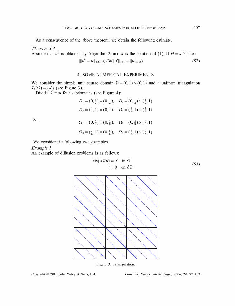
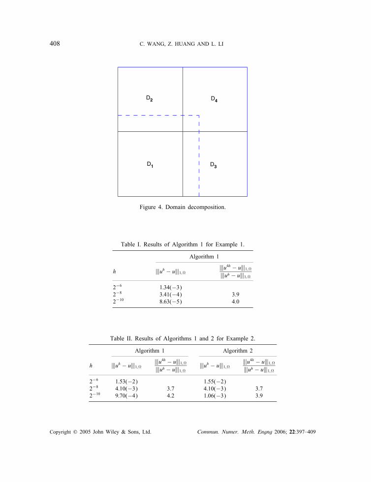
We consider the simple unit square domain �= (0; 1)× (0; 1) and a uniform triangulationTh(�)= {K} (see Figure 3).Divide � into four subdomains (see Figure 4):

D1 = (0; 12 )× (0; 12 ); D2 = (0; 12 )× ( 12 ; 1)D3 = (12 ; 1)× (0; 12 ); D4 = (12 ; 1)× ( 12 ; 1)

Set�1 = (0; 58 )× (0; 58 ); �2 = (0; 58 )× ( 38 ; 1)

�3 = (38 ; 1)× (0; 58 ); �4 = (38 ; 1)× ( 38 ; 1)

We consider the following two examples:Example 1An example of di�usion problems is as follows:

−div(A∇u) =f in �u=0 on @�

(53)

Figure 3. Triangulation.



D1

D2 D4

D3

Figure 4. Domain decomposition.

Table I. Results of Algorithm 1 for Example 1.

Algorithm 1

h |‖uh − u|‖1;� |‖u4h − u|‖1;�|‖uh − u|‖1;�

2−6 1:34(−3)2−8 3:41(−4) 3.92−10 8:63(−5) 4.0

Table II. Results of Algorithms 1 and 2 for Example 2.

Algorithm 1 Algorithm 2

h |‖uh − u|‖1;� |‖u4h − u|‖1;�|‖uh − u|‖1;� |‖uh − u|‖1;� |‖u4h − u|‖1;�

|‖uh − u|‖1;�2−6 1:53(−2) 1:55(−2)2−8 4:10(−3) 3.7 4:10(−3) 3.72−10 9:70(−4) 4.2 1:06(−3) 3.9



where A=(aij)2× 2, and a11 = ey, a22 = 1, a12 = a21 = 0, f= − 6(1 − x)x3(1 − y)y+ 6(1− x)x3y2 − ey(6(1− x)x(1− y)y3 − 6x2(1− y)y3).Example 2An example of convection–di�usion problems is as follows:

−div(A∇u+ bu) + cu=f in �

u=0 on @�(54)

where A=(aij)2× 2, and a11 = 1, a22 = 1, a12 = a21 = 0, b=[y; x]t , c=200, f= − �y cos(�x)sin(�y)− �x sin(�x) cos(�y) + 2�2 sin(�x) sin(�y) + 200 sin(�x) sin(�y).We shall apply Algorithms 1 and 2 to solve these problems, using �ne grids of sizes

h=2−j ( j=6; 8; 10) and corresponding coarse grids of size H = h1=2. Tables I and II indicatethat the computational results coincide with the theory established before.

REFERENCES

1. Chou SH, Li Q. Error estimates in L2, H 1 and L∞ in covolume methods for elliptic and parabolic problem:a uni�ed approach. Mathematics of Computation 2000; 209:103–120.

2. Chou SH. Analysis and convergence of a covolume method for the generalized stokes problem. NumerischeMathematik 1997; 55:85–104.

3. Chou SH, Kwak DY, Vassilerski PS. Mixed covolume methods for elliptic problems on triangular grids. SIAMJournal on Numerical Analysis 1998; 35:1850–1861.

4. Cartr�es R, Herbin R, Hubert F. Nonmatching �nite volume grids and the nonoverlapping Schwarz algorithm.In Thirteenth International Conference on Domain Decomposition Methods, Debit N, Garbey M, Hoppe R,P�eriaux J, Keyes D, Kuznetsov Y (eds). ddm.org, 2001.

5. Chou SH, Kwak DY. Multigrid algorithms for a vertex-centered covolume method for elliptic problems.Numerische Mathematik 2002; 90:441–458.

6. Ewing RE, Lazarov RD, Lin T, Lin Y. Mortar �nite volume element approximations of second order ellipticproblems. Technical Report ISC-99-08-MATH, Texas A&M University, East-West Journal of NumericalMathematics 2000; 8:93–110.

7. Xu JC. A new class of iterative methods for nonselfadjoint or inde�nite problems. SIAM Journal on NumericalAnalysis 2000; 29:303–319.

8. Xu JC. Two-grid discretization techniques for linear and nonlinear PDEs. SIAM Journal on Numerical Analysis1996; 33:1759–1777.

9. Axelsson O, Layton VV. A two-level discretization of nonlinear boundary value problems. SIAM Journal onNumerical Analysis 1996; 33:2359–2374.

10. Xu JC, Zhou AH. Local and parallel �nite element algorithms based on two-grid discretizations. Mathematicsof Computation 1999; 69:881–909.

11. Dawson CN, Wheeler MF. Two-grid methods for mixed �nite element approximations of nonlinear parabolicequations. Contemporary Mathematics 1994; 180:191–203.

12. Dawson CN, Wheeler MF, Woodward CS. A two-grid �nite di�erence scheme for nonlinear parabolic equations.SIAM Journal on Numerical Analysis 1998; 35:435–452.

13. Marion M, Xu JC. Error estimates on a new nonlinear Galerkin method based on two-grid �nite elements.SIAM Journal on Numerical Analysis 1995; 32:1170–1184.

14. Ewing RE, Lin T, Lin Y. On the accuracy of the �nite volume element method based on piecewise linearpolynomials. SIAM Journal on Numerical Analysis 2002; 39:1865–1888.

15. Ciarlet PG. The Finite Element Method for Elliptic Problems. North-Holland: Amsterdam, 1978.16. Brenner SC, Scott LR. The Mathematical Theory of Finite Element Methods. Springer: New York, Berlin,

Heidelberg, 1994.


Documents

Two-grid covolume schemes for elliptic problems