Two-machine flowshop scheduling problem to minimize total completion time with bounded setup and processing times

ARTICLE IN PRESS

0925-5273/$ - se

doi:10.1016/j.ijp

�CorrespondiE-mail addre

Int. J. Production Economics 103 (2006) 386–400

www.elsevier.com/locate/ijpe

Two-machine flowshop scheduling problem to minimize totalcompletion time with bounded setup and processing times

Ali Allahverdi�

Department of Industrial and Management Systems Engineering, College of Engineering and Petroleum, Kuwait University,

P.O. Box 5969, Safat, Kuwait

Received 4 November 2004; accepted 13 October 2005

Available online 20 February 2006

Abstract

The two-machine flowshop scheduling problem is addressed where setup times are considered as separate from

processing times and where the objective is to minimize total completion time. All setup and processing times on both

machines are unknown variables (before the actual occurrence of these times) where the only known information is the

lower and upper bounds for both setup and processing times of each job. In such an environment, there may not exist a

unique schedule that remains optimal for all possible realizations of setup and processing times, and therefore, a set of

dominating schedules (which dominate all other schedules) has to be obtained. The objective in such a scheduling

environment is to reduce the size of dominating schedules set. Two dominance relations are developed for the considered

problem. Illustrative numerical examples are given and computational experiments on randomly generated problems are

conducted. The computational experiments show that the developed dominance relations are quite helpful in reducing the

size of dominating schedules.

r 2006 Elsevier B.V. All rights reserved.

Keywords: Scheduling; Flowshop; Bounded processing times; Bounded setup times; Dominance relations

1. Introduction

The vast majority of research on flowshop scheduling problems assumes that job processing times areknown fixed values in advance. There are many problems in real life where job processing times can bemodeled as known fixed values. It is not realistic, however, to assume they are known fixed values for someother scheduling problems. For such scheduling environments, job processing times are unknown variablesand the only information that can be obtained is about lower and upper bounds for each job, which is calledbounded processing times. Allahverdi and Sotskov (2003) addressed the two-machine flowshop schedulingproblem to minimize makespan when job processing times are bounded. Sotskov et al. (2004) addressed thesame problem but with total completion time criterion. Both Allahverdi and Sotskov (2003), and Sotskovet al. (2004) assumed that setup times are included in processing times.

e front matter r 2006 Elsevier B.V. All rights reserved.

e.2005.10.002

ng author. Tel.: +965 4987874; fax: +965 484 6137.

ss: [email protected].

www.elsevier.com/locate/ijpe

ARTICLE IN PRESSA. Allahverdi / Int. J. Production Economics 103 (2006) 386–400 387

The assumption of including setup times in processing times is a common assumption in the flowshopscheduling research. While this assumption may be justified for some real scheduling problems, othersituations call for explicit (separate) setup time consideration. For example, the production of seamless steeltube in iron and steel industries (Tang and Huang, 2005) or group scheduling in flexible flowshops (Logendranet al., 2005). The practical situations in which setup times must be considered as separate include chemical,pharmaceutical, printing, food processing, metal processing, and semiconductor industries, see Allahverdiet al. (1999) for a survey on the scheduling problems with separate setup times. An obvious advantage ofconsidering setup times separate for our problem is that when there exists some idle time on the secondmachine (usually the case), then the setup time for a job on the second machine can be performed prior to thecompletion time of this job on the first machine. This means that the performance measure may be improvedby considering setup times as separate from processing times. Hence, some researchers considered theflowshop problem with separate setup times, i.e., relaxing the assumption that setup times are included inprocessing times. Bagga and Khurana (1986) and Allahverdi (2000) addressed the two-machine separate setuptime problem with respect to total completion time criterion. Although Bagga and Khurana (1986) andAllahverdi (2000) considered setup times as separate from processing times, they assumed setup times to bedeterministic, i.e., known before scheduling and fixed during a realization of the process. In reality, thisassumption is not valid for some cases, and therefore, setup times have to be considered as unknown variables.Allahverdi et al. (2003) considered the two-machine flowshop scheduling problem to minimize totalcompletion time with bounded setup times but where job processing times are assumed to be known fixedvalues.

In this paper, we address the two-machine flowshop scheduling problem to minimize total completion timewith unknown setup and unknown processing times where only lower and upper bounds for setup andprocessing times of each job are known before scheduling takes place. It has been observed that although theexact values of setup and processing times may not be known before scheduling, some upper and lowerbounds on job setup and processing times are easy to obtain in most practical cases. This information on thebounds of setup and processing times is important, and hence, it should be utilized in finding a solution for thescheduling problem.

The rest of this paper is organized as follows. Problem description is given in Section 2. Some dominancerelations are developed in Sections 3, and numerical examples are given in Section 4. Computational analysisof the developed dominance relations is conducted in Section 5 and concluding remarks are made in Section 6.

2. Problem description

We consider the two-machine flowshop scheduling problem in which job processing times are unknownvariables where only a lower bound LBtj,mX0 and an upper bound UBtj,mXLBtj,m of the processing time tj,m

of job j on machine m are given before scheduling. Moreover, before scheduling, setup times are also unknownvariables with a lower bound LBsj,mX0 and an upper bound UBsj,mX LBsj,m of the setup time sj,m of job j onmachine m. Such a flowshop problem can be denoted as F2jLBtj;mptj;mpUBtj;m; LBsj;mpsj;mpUBsj;mjSCj

where the first term denotes that it is a two-machine flowshop, the second term indicates that both processingand setup times are unknown variables with some lower and upper bounds, and the last term specifies that theobjective of the problem is to minimize the total completion time of all jobs. Notice that the problemF2jLBtj;mptj;mpUBtj;m; LBsj;mpsj;mpUBsj;mjSCj can be considered as a stochastic flowshop problem underuncertainty of setup and processing times when there is no prior information about probability distributionsof the random setup and processing times. It is only known that setup and processing times of each job will fallbetween some given lower and upper bounds with probability one. Similar problems have been addressed inthe literature for the case where job processing times are random variables but setup times are assumed to bezero, see Lai et al. (1997), Lai and Sotskov (1999), Allahverdi and Sotskov (2003), and Sotskov et al. (2004).Also Allahverdi et al. (2003) addressed the problem for the case where job processing times are fixed values butsetup times are separate and random variables with lower and upper bounds.

If the equalities LBsj;m ¼ sj;m ¼ UBsj;m and LBtj;m ¼ tj;m ¼ UBtj;m hold for each job j 2 J and eachmachine m 2M where J ¼ f1; 2; . . . ; ng denotes the set of jobs and M ¼ f1; 2g denotes the set of machines,then the problem F2jLBtj;mptj;mpUBtj;m; LBsj;mpsj;mpUBsj;mjSCj reduces to the flowshop problem F2jtj;m;

ARTICLE IN PRESSA. Allahverdi / Int. J. Production Economics 103 (2006) 386–400388

sj;mjP

Cj with fixed setup and processing times that was considered by Bagga and Khurana (1986) andAllahverdi (2000). It should be noted that the F2jtj;m; sj;mjSCj problem is known to be NP-hard, see Gonzalezand Sahni (1978). Therefore, the problem of F2jLBtj;mptj;mpUBtj;m; LBsj;mpsj;mpUBsj;mjSCj is also NP-hard, meaning that it is highly unlikely to find a polynomial time algorithm to solve the problem. It shouldalso be noted that even if the problem of F2jtj;m; sj;mSCj were to have a polynomial time solution, it might notstill be possible to find an optimal solution for the problem of F2jLBtj;mptj;mpUBtj;m; LBsj;mpsj;mpUBsj;mjSCj since the optimality of a solution depends on the realization of setup and processing times. Theonly possible case is when the set of optimal (dominating) solution contains only one sequence in which casethe sequence will remain optimal regardless of the setup and processing times realization with possiblydifferent objective function values. That is, the objective function value depends on the realization of setupand processing times.

Setup time is called sequence-independent if it depends only on the job to be processed. On the other hand, ifthe setup time depends on both the job to be processed and the immediately preceding job, then it is calledsequence-dependent. When setup times are sequence-independent on both machines, then permutation

schedules are dominant with respect to any regular criterion, see Yoshida and Hitomi (1979). Thus, in order tofind an optimal schedule one only needs to consider the same sequence of jobs on both machines. In theproblem F2jLBtj;mptj;mpUBtj;m; LBsj;mpsj;mpUBsj;mjSCj under consideration, we assume that setup timesare sequence-independent on both machines, and hence, permutation schedules are dominant with respect tothe total completion time criterion. Therefore, we only consider the set of permutation schedules, and there aren! sequences (permutations) F ¼ F1;F2; . . . ;Fn!f g for the problem of F2jLBtj;mptj;mpUBtj;m; LBsj;mpsj;mpUBsj;mjSCj that will be considered in finding the optimal solution.

Let the bracket [i,m] denote the job in position i on machine m. For example, t[i,m] denotes the processingtime of the job in position i on machine m. For the deterministic version of the problem where processing andsetup times are fixed (i.e., LBtj;m ¼ tj;m ¼ UBtj;m and LBsj;m ¼ sj;m ¼ UBsj;m), Yoshida and Hitomi (1979)established the following formula for the completion time C[j] of the job in position j:

C½j� ¼ max0pupj

Xu

i¼1

ðs½i;1� � s½i;2� þ t½i;1�Þ �Xu�1i¼1

t½i;2�

" #þXj

i¼1

ðs½i;2� þ t½i;2�Þ:

The above equation can be written as follows:

C½j� ¼ max0pupj

Xu

i¼1

ðs½i;1� þ t½i;1�Þ �Xu�1i¼1

ðs½i;2� þ t½i;2�Þ � s½u;2�

" #þXj

i¼1

ðs½i;2� þ t½i;2�Þ:

¼ max0pupj

½TSP½u;1� � ðTSP½u�1;2� þ s½u;2��Þ þ TSP½j;2�,

where we use the notation TSP½j;m� ¼Pj

r¼1ðs½r;m� þ t½r;m�Þ, for j ¼ 1; 2; . . . ; n and m 2M ¼ f1; 2g.Let, Dj ¼ maxf0; d1; d2; . . . ; djg where dj ¼ TSP½j;1� � ðTSP½j�1;2� þ s½j;2�Þ, j ¼ 1; 2; . . . ; n, where TSP½0;2� ¼ 0.

Then, C[j] can be written as C½j� ¼ TSP½j;2� þ Dj. The term Dj denotes the total idle time on the second machineuntil the job in position j is completed. Once completion times of all n jobs are known, then the totalcompletion time, TCT, is obtained as follows:

TCT ¼Xn

j¼1

ðTSP½j;2� þ DjÞ:

For each job j 2 J and machine m 2M, any feasible realization tj,m of processing times satisfies theinequalities: LBtj,mptj,mpUBtj,m. Similarly, any feasible realization sj,m of setup time satisfies the inequalities:LBsj,mpsj,mpUBsj,m. Before scheduling, we only know the lower and upper bounds of processing and setuptimes given by the above inequalities, which define polytope PT of feasible vectors t ¼ ðt1;1; t1;2; t2;1; t2;2; . . . ;tn;1; tn;2Þ and s ¼ ðs1;1; s1;2; s2;1; s2;2; . . . ; sn;1; sn;2Þ of processing and setup times as follows: PT ¼ ft : LBtj;mptj;mpUBtj;m, and s : LBsj;mpsj;mpUBsj;m, j 2 J, m 2Mg.

Similar to Lai and Sotskov (1999), we use the following definition of a solution to the problemF2jLBtj;mptj;mpUBtj;m;LBsj;mpsj;mpUBsj;mjSCj. A set of sequences F� � F is a solution to the problemF2jLBtj;mptj;mpUBtj;m; LBsj;mpsj;mpUBsj;mjSCj if for each feasible vector tAPT of processing times and


each feasible vector sAPT of setup times, the set F� contains at least one optimal sequence. Thus, the whole setF of sequences is a trivial solution for the problem F2jLBtj;mptj;mpUBtj;m;LBsj;mpsj;mpUBsj;mjSCj.However, it is only possible to construct the whole set F for a small number of jobs. It is also impractical tochoose the best sequence from a large set F� of candidates as the processing and setup times of jobs evolves.Therefore, it is important to minimize the cardinality of solution F� constructed for the problemF2jLBtj;mptj;mpUBtj;m;LBsj;mpsj;mpUBsj;mjSCj . We introduce the following dominance relations on theset of sequences F.

Definition. For the problem F2jLBtj;mptj;mpUBtj;m;LBsj;mpsj;mpUBsj;mjSCj a sequence F1 2 F dominatesa sequence F2 2 F with respect to PT if the inequality TCTðF1ÞpTCTðF2Þ holds for any vectors tAPT andsAPT.

By the above definition, a set of sequences F� � F is a solution to the problem F2jLBtj;mptj;mpUBtj;m;LBsj;mpsj;mpUBsj;mjSCj if for each sequence Fk 2 F, there exists a sequence from the set F� that dominatesthe sequence Fk with respect to PT.

3. Dominance relations

Let fh denote a subsequence of a complete sequence Fu 2 F of all the n jobs. Therefore, the notations ofF1 ¼ ðf1; i;f2; k;f3Þ and F2 ¼ ðf1; k;f2; i;f3Þ mean that the two sequences of F1 2 F and F2 2 F have thesame jobs in all positions except that the jobs i 2 J and k 2 J are interchanged. When the jobs i and k areadjacent, such two complete sequences of F3 2 F and F4 2 F can be expressed as follows F3 ¼ ðf1; i; k;f2Þ

and F4 ¼ ðf1; k; i;f2Þ.

Theorem 1. For the problem F2jLBtj;mptj;mpUBtj;m;LBsj;mpsj;mpUBsj;mjSCj, the sequence F1 ¼

ðf1; i;f2; k;f3Þ 2 F dominates the sequence F2 ¼ ðf1; k;f2; i;f3Þ 2 F with respect to PT if the following three

inequalities hold:

UBtk;2pLBti;2,

UBsi;2 þUBti;2pLBsk;2 þ LBtk;2 and

UBsi;1 þUBti;1 þUBsk;2pLBsk;1 þ LBtk;1 þ LBsi;2.

Proof. We consider two job sequences F1 and F2 where F1 is a sequence in which job i is in position a and jobk in position b, where aob, whereas sequence F2 is obtained from sequence F1 by interchanging only the jobsin positions a and b. When necessary, we attach a corresponding sequence Fu 2 F to the notations C½j�, Dj, dj ,TSP½j;j�, TCT, i.e., C½j�ðFuÞ, DjðFuÞ, djðFuÞ, TSP½j;j� ðFuÞ, TCTðFuÞ.

It should be clear that TSP[a�1,1](F1) ¼ TSP[a�1,1](F2) and TSP[a�1,2](F1) ¼ TSP[a�1,2](F2) since bothsequences have the same job in each position 1,2,y,a�1. For j ¼ a, we obtain

daðF1Þ ¼ TSP½a�1;1�ðF1Þ þ si;1 þ ti;1 � ðTSP½a�1;2�ðF1Þ þ si;2Þ,

daðF2Þ ¼ TSP½a�1;1�ðF2Þ þ sk;1 þ tk;1 � ðTSP½a�1;2�ðF2Þ þ sk;2Þ.

From the above two equalities we obtain

daðF1ÞpdaðF2Þ (1)

since for all realizations of setup and processing times UBsi;1 þUBti;1 þUBsk;2pLBsk;1 þ LBtk;1 þ LBsi;2

always implies that si;1 þ ti;1 þ sk;2psk;1 þ tk;1 þ si;2.In other words, regardless of which values si;1; ti;1; sk;2; sk;1; tk;1, and si,2 take, it is always true that si;1 þ

ti;1 þ sk;2psk;1 þ tk;1 þ si;2 as long as UBsi;1 þUBti;1 þUBsk;2pLBsk;1 þ LBtk;1 þ LBsi;2 is satisfied. Note thatbefore scheduling (i.e., before jobs are processed) we do not know the exact values of si;1; ti;1; sk;2; sk;1; tk;1, and


si,2, However, we are assured that daðF1ÞpdaðF2Þ as long as UBsi;1 þUBti;1 þUBsk;2pLBsk;1 þ LBtk;1 þ

LBsi;2 holds. This argument is valid for all the cases to be considered throughout the paper. For brevity it willnot be repeated.

For j ¼ a+1, a+2,y,b�1, we obtain

djðF1Þ ¼ TSP½a�1;1�ðF1Þ þ si;1 þ ti;1 þXj

r¼aþ1

ðs½r;1� þ t½r;1�Þ

� TSP½a�1;2�ðF1Þ þ si;2 þ ti;2 þXj�1

r¼aþ1

ðs½r;2� þ t½r;2�Þ þ s½j;2�

" #,

djðF2Þ ¼ TSP½a�1;1�ðF2Þ þ sk;1 þ tk;1 þXj

r¼aþ1

ðs½r;1� þ t½r;1�Þ

� TSP½a�1;2�ðF2Þ þ sk;2 þ tk;2 þXj�1

r¼aþ1

ðs½r;2� þ t½r;2�Þ þ s½j;2�

" #,

wherePa

r¼aþ1ðs½r;2� þ t½r;2�Þ ¼ 0. Both sequences have the same job in all positions up to position b�1 except forposition a, hence, it follows that djðF1Þ � djðF2Þ ¼ ðsi;1 þ ti;1 þ sk;2Þ � ðsk;1 þ tk;1 þ si;2Þ þ tk;2 � ti;2. ButUBtk;2pLBti;2 implies that tk,2pti,2, and UBsi;1 þUBti;1 þUBsk;2pLBsk;1 þ LBtk;1 þ LBsi;2 implies thatsi;1 þ ti;1 þ sk;2psk;1 þ tk;1 þ si;2. Therefore,

djðF1ÞpdjðF2Þ. (2)

For j ¼ b, we obtain

dbðF1Þ ¼ TSP½a�1;1�ðF1Þ þ si;1 þ ti;1 þXb�1

r¼aþ1

ðs½r;1� þ t½r;1�Þ þ sk;1 þ tk;1

� TSP½a�1;2�ðF1Þ þ si;2 þ ti;2 þXb�1

r¼aþ1

þðs½r;2� þ t½r;2�Þ þ sk;2

" #,

dbðF2Þ ¼ TSP½a�1;1�ðF2Þ þ sk;1 þ tk;1 þXb�1

r¼aþ1

ðs½r;1� þ t½r;1�Þ þ si;1 þ ti;1

� TSP½a�1;2�ðF2Þ þ sk;2 þ tk;2 þXb�1

r¼aþ1

þðs½r;2� þ t½r;2�Þ þ si;2

" #.

It follows from the last two equalities that

dbðF1ÞpdbðF2Þ, (3)

since UBtk;2pLBti;2 implies that tk;2pti;2.It is obvious that djðF1Þ ¼ djðF2Þ for each j ¼ 1; 2; . . . ; a� 1 since both sequences have the same job in these

positions. It can easily be shown that djðF1Þ ¼ djðF2Þ for each j ¼ bþ 1, bþ 2; . . . ; n. From these facts and(1)–(3), we obtain

djðF1ÞpdjðF2Þ (4)

for each position j ¼ 1; 2; . . . ; n.Observe that

C½j�ðF1Þ ¼ C½j�ðF2Þ (5)


for each position j ¼ 1; 2; . . . ; a� 1, since both sequences have the same job in these positions. It is obviousthat Da�1ðF1Þ ¼ Da�1ðF2Þ. It can easily be shown that for each position j ¼ b, bþ 1; . . . ; n

C½j�ðF1Þ � C½j�ðF2Þ ¼ maxfDa�1ðF1Þ; daðF1Þ; daþ1ðF1Þ; . . . ; djðF1Þg

�maxfDa�1ðF2Þ; daðF2Þ; daþ1ðF2Þ; . . . ; djðF2Þg,

But it follows from (4) that

maxfDa�1ðF1Þ; daðF1Þ; daþ1ðF1Þ; . . . ; djðF1ÞgpmaxfDa�1ðF2Þ; daðF2Þ; daþ1ðF2Þ; . . . ; djðF2Þg,

and therefore,

C½j�ðF1ÞpC½j�ðF2Þ (6)

for each position j ¼ b, bþ 1; :::; n. Observe that for j ¼ a,

C½a�ðF1Þ ¼ TSP½a�1;2�ðF1Þ þ si;2 þ ti;2 þmaxfDa�1ðF1Þ; daðF1Þg,

C½a�ðF2Þ ¼ TSP½a�1;2�ðF2Þ þ sk;2 þ tk;2 þmaxfDa�1ðF2Þ; daðF2Þg

and for j ¼ aþ 1, aþ 2; :::; b� 1

C½j�ðF2Þ ¼ TSP½a�1;2�ðF2Þ þ sk;2 þ tk;2 þXj

r¼aþ1

ðs½r;2� þ t½r;2� þmaxfDa�1ðF2Þ; daðF2Þ; daþ1ðF2Þ; . . . ; djðF2Þg,

C½j�ðF1Þ ¼ TSP½a�1;2�ðF1Þ þ si;2 þ ti;2 þXj

r¼aþ1

ðs½r;2� þ t½r;2� þmaxfDa�1ðF1Þ; daðF1Þ; daþ1ðF1Þ; . . . ; djðF1Þg.

Hence, for each position j ¼ a, aþ 1; :::; b� 1, we obtain

C½j�ðF1Þ � C½j�ðF2Þ ¼ ðsi;2 þ ti;2Þ � ðsk;2 þ tk;2Þ þmaxfDa�1ðF1Þ; . . . ; djðF1Þg �maxfDa�1ðF2Þ; . . . ; djðF2Þg.

However, UBsi;2 þUBti;2pLBsk;2 þ LBtk;2 implies that si;2 þ ti;2psk;2 þ tk;2 and by (6), maxfDa�1ðF1Þ; :::;djðF1ÞgpmaxfDa�1ðF2Þ; :::; djðF2Þg, and therefore,


for each j ¼ a, aþ 1; :::; b� 1. Now it follows from (5)–(7) that the sequence F1 ¼ ðf1; i;f2; k;f3Þ 2 Fdominates the sequence F2 ¼ ðf1; k;f2; i;f3Þ 2 F with respect the performance measure of total completiontime. In other words, TCTðF1ÞpTCTðF2Þ. This completes the proof. &

The dominance relation given in Theorem 1 is called a global dominance relation since when the specifiedrelations hold, say, for jobs h and g (h precedes g), then regardless of the positions of h and g, in an optimalsolution job h precedes job g even if they are not adjacent. The relations given in the following theorem iscalled a local dominance relation. That is because when the specified relations hold, say, for jobs h and g (hprecedes g), then job h precedes job g in an optimal solution only when both jobs are adjacent. Notice that aglobal dominance relation helps in reducing the search space more than a local dominance relation.

Theorem 2. For the problem F2jLBtj;mptj;mpUBtj;m; LBsj;mpsj;mpUBsj;mjP

Cj, the sequence F3 ¼

ðf1; i; k;f2Þ 2 F dominates the sequence F4 ¼ ðf1; k; i;f2Þ 2 F with respect to PT if the inequalities

(i)
UBsi;1 þUBti;1 þUBsk;2pLBsk;1þ LBtk;1 þ LBsi;2, (ii) UBsi;2 þUBti;2pLBsk;2 þ LBtk;2
and one of the following inequalities hold:

(iiia)
UBsk;1 þUBtk;1pLBti;2 þ LBsk;2, (iiib) UBsi;1 þUBti;1pLBsi;2 þ LBti;2, (iiic) UBtk;2pLBti;2.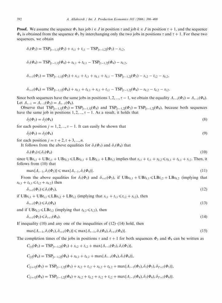

Proof. We assume the sequence F3 has job i 2 J in position t and job k 2 J in position tþ 1, and the sequenceF4 is obtained from the sequence F3 by interchanging only the two jobs in positions t and tþ 1. For these two
sequences, we obtain
dtðF3Þ ¼ TSP½t�1;1�ðF3Þ þ si;1 þ ti;1 � TSP½t�1;2�ðF3Þ � si;2,

dtðF4Þ ¼ TSP½t�1;1�ðF4Þ þ sk;1 þ tk;1 � TSP½t�1;2�ðF4Þ � sk;2,

dtþ1ðF3Þ ¼ TSP½t�1;1�ðF3Þ þ si;1 þ ti;1 þ sk;1 þ tk;1 � TSP½t�1;2�ðF3Þ � si;2 � ti;2 � sk;2,

dtþ1ðF4Þ ¼ TSP½t�1;1�ðF4Þ þ sk;1 þ tk;1 þ si;1 þ ti;1 � TSP½t�1;2�ðF4Þ � sk;2 � tk;2 � si;2.

Since both sequences have the same jobs in positions 1; 2; :::; t� 1, we obtain the equality Dt�1ðF3Þ ¼ Dt�1ðF4Þ.Let Dt�1 ¼ Dt�1ðF3Þ ¼ Dt�1ðF4Þ.

Observe that TSP½t�1;1�ðF3Þ ¼ TSP½t�1;1�ðF4Þ and TSP½t�1;2�ðF3Þ ¼ TSP½t�1;2�ðF4Þ, because both sequenceshave the same job in positions 1; 2; :::; t� 1. As a result, it holds that

djðF3Þ ¼ djðF4Þ (8)

for each position j ¼ 1; 2; :::; t� 1. It can easily be shown that

djðF3Þ ¼ djðF4Þ (9)

for each position j ¼ tþ 2; tþ 3; :::; n.It follows from the above equalities for dtðF3Þ and dtðF4Þ that

dtðF3ÞpdtðF4Þ (10)

since UBsi;1 þUBti;1 þUBsk;2pLBsk;1 þ LBtk;1 þ LBsi;2 implies that si;1 þ ti;1 þ sk;2psk;1 þ tk;1 þ si;2. Then, itfollows from (10) that

maxfDt�1; dtðF3ÞgpmaxfDt�1; dtðF4Þg. (11)

From the above equalities for dtðF3Þ and dtþ1ðF3Þ, if UBsk;1 þUBtk;1pLBti;2 þ LBsk;2 (implying thatsk;1 þ tk;1pti;2 þ sk;2) then

dtþ1ðF3ÞpdtðF3Þ, (12)

if UBsi;1 þUBti;1pLBsi;2 þ LBti;2 (implying that si;1 þ ti;1pti;2 þ si;2), then

dtþ1ðF3ÞpdtðF4Þ (13)

and if UBtk;2pLBti;2 (implying that tk;2pti;2), then

dtþ1ðF3Þpdtþ1ðF4Þ. (14)

If inequality (10) and any one of the inequalities of (12)–(14) hold, then

maxfDt�1; dtðF3Þ; dtþ1ðF3ÞgpmaxfDt�1; dtðF4Þ; dtþ1ðF4Þg. (15)

The completion times of the jobs in positions t and tþ 1 for both sequences F3 and F4 can be written as

C½t�ðF3Þ ¼ TSP½t�1;2�ðF3Þ þ si;2 þ ti;2 þmaxfDt�1ðF3Þ; dtðF3Þg,

C½t�ðF4Þ ¼ TSP½t�1;2�ðF4Þ þ sk;2 þ tk;2 þmaxfDt�1ðF4Þ; dtðF4Þg,

C½tþ1�ðF3Þ ¼ TSP½t�1;2�ðF3Þ þ si;2 þ ti;2 þ sk;2 þ tk;2 þmaxfDt�1ðF3Þ; dtðF3Þ; dTþ1ðF3Þg,

C½tþ1�ðF4Þ ¼ TSP½t�1;2�ðF4Þ þ sk;2 þ tk;2 þ si;2 þ ti;2 þmaxfDt�1ðF4Þ; dtðF4Þ; dTþ1ðF4Þg.



Taking the difference between completion times of the jobs in positions t and tþ 1 for the two sequencesyields

½C½t�ðF3Þ þ C½tþ1�ðF3Þ� � ½C½t�ðF4Þ þ C½tþ1�ðF4Þ� ¼ ðsi;2 þ ti;2Þ � ðsk;2 þ tk;2Þ

þmaxfDt�1; dtðF3Þg �maxfDt�1; dtðF4Þg þmaxfDt�1; dtðF3Þ; dtþ1ðF3Þg �maxfDt�1; dtðF4Þ; dtþ1ðF4Þg.

From (11), (15), and the fact that UBsi;2 þUBti;2pLBsk;2 þ LBtk;2 we obtain

C½t�ðF3Þ þ C½tþ1�ðF3ÞpC½t�ðF4Þ þ C½tþ1�ðF4Þ. (16)

It can also be shown that for each position j ¼ tþ 2, tþ 3; :::; n,

C½j�ðF3Þ � C½j�ðF4Þ ¼ maxfDt�1; dtðF3Þ; dtþ1ðF3Þ; dtþ2ðF3Þ; . . . ; djðF3Þg

�maxfDt�1; dtðF4Þ; dtþ1ðF4Þ; dtþ2ðF4Þ; . . . ; djðF4Þg.

We observe that dkðF3Þ ¼ dkðF4Þ for each k ¼ tþ 2, tþ 3; . . . ; n. Therefore, from the inequalities of (8), (9),and (15) we obtain


for each position j ¼ tþ 2, tþ 3; . . . ; n. It is obvious that

C½j�ðF3Þ ¼ C½j�ðF4Þ (18)

for each j ¼ 1; 2; . . . ; t� 1. Clearly from (16)–(18), we obtain the inequality TCTðF3ÞpTCTðF4Þ whichcompletes the proof. &

Table 1

Bounds for setup and processing times of example 1

Job j LBsj;1 UBsj:1 LBsj;2 UBsj;2 LBtj;1 UBtj;1 LBtj;2 UBtj;2

1 1 4 4 6 6 9 8 12

2 3 8 5 8 5 10 4 9

3 2 4 1 4 2 6 7 11

4 4 8 5 7 3 5 8 10

Table 2

Three possible realizations for example 1

Realization Job j sj;1 tj;1 sj;2 tj;2

1 1 2 7 5 9

2 5 6 6 5

3 3 3 3 8

4 6 5 6 9

2 1 4 8 4 8

2 7 9 5 4

3 3 5 1 7

4 6 5 6 8

3 1 1 6 6 10

2 4 5 7 8

3 2 3 3 9

4 5 4 7 9


4. Numerical examples

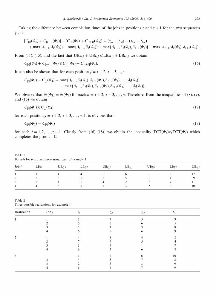
Consider the four-job problem given in Table 1 where lower and upper bounds for both setup andprocessing times of each job are given. Note that these are bounds and we do not know the exact values untilthe processing of all jobs is completed. We would like to obtain (if possible) the optimal solution or reduce thesize of the set which contain the optimal solution by applying the developed dominance relations.

Theorem 1 implies the following precedence relations in an optimal solution for a feasible vector s 2 PT ofsetup times and a feasible vector t 2 PT of processing times, polytope PT being defined in Table 1. Accordingto Theorem 1, jobs 1, 2, and 3 precede job 4 in an optimal solution. This indicates that job 4 has to be in thelast position since the only possible way that jobs 1, 2, and 3 precede job 4 is by placing jobs 1, 2, and 3 in thefirst three positions. In other words, we have a partial sequence as F ¼ ð�;�;�; 4Þ. Moreover, jobs 2 and 3precede job 1 in an optimal solution, which again is as a result of Theorem 1. This shows that job 1 has to be inthe second last position, which leads to the partial sequence of F ¼ ð�;�; 1; 4Þ. The first two positions will beoccupied by jobs 2 and 3. However, it follows from Theorem 2 that job 3 precedes job 2 in an optimal solution.Therefore, we are able to construct a complete sequence as F ¼ ð3; 2; 1; 4). This sequence is the optimalsolution. It should be noted that there are many possible problem sets that can result in from the data given inTable 1. In other words, the sequence F ¼ ð3; 2; 1; 4Þ is optimal regardless of the possible realization of setupand processing times which will be only known once the schedule is complete since both setup and processingtimes evolve as the schedule progresses. Three possible realizations of setup and processing times are given inTable 2. Notice that for each realization, both setup and processing times are within the lower and upperbounds given in Table 1. The optimal sequence is the same as F ¼ ð3; 2; 1; 4Þ for each realization. However, theobjective function value for each realization will probably be different. For the realizations given in Table 2,the total completion times for the optimal sequence F ¼ ð3; 2; 1; 4Þ are 132, 145, and 149 for realizations 1, 2,and 3, respectively.

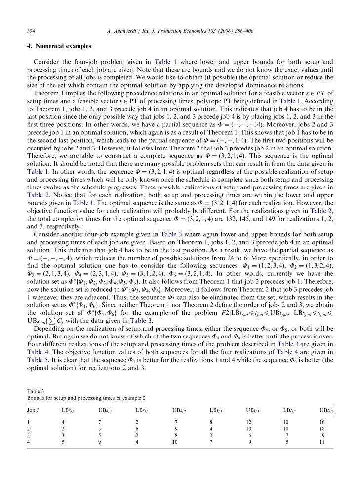
Consider another four-job example given in Table 3 where again lower and upper bounds for both setupand processing times of each job are given. Based on Theorem 1, jobs 1, 2, and 3 precede job 4 in an optimalsolution. This indicates that job 4 has to be in the last position. As a result, we have the partial sequence asF ¼ ð�;�;�; 4Þ, which reduces the number of possible solutions from 24 to 6. More specifically, in order tofind the optimal solution one has to consider the following sequences: F1 ¼ ð1; 2; 3; 4Þ, F2 ¼ ð1; 3; 2; 4Þ,F3 ¼ ð2; 1; 3; 4Þ, F4 ¼ ð2; 3; 1; 4Þ, F5 ¼ ð3; 1; 2; 4Þ, F6 ¼ ð3; 2; 1; 4Þ. In other words, currently we have thesolution set as F�fF1;F2;F3;F4;F5;F6g. It also follows from Theorem 1 that job 2 precedes job 1. Therefore,now the solution set is reduced to F�fF3;F4;F6g. Moreover, it follows from Theorem 2 that job 3 precedes job1 whenever they are adjacent. Thus, the sequence F3 can also be eliminated from the set, which results in thesolution set as F�fF4;F6g. Since neither Theorem 1 nor Theorem 2 define the order of jobs 2 and 3, we obtainthe solution set of F�fF4;F6g for the example of the problem F2jLBtj;mptj;mpUBtj;m; LBsj;mpsj;mpUBsj;mj

PCj with the data given in Table 3.

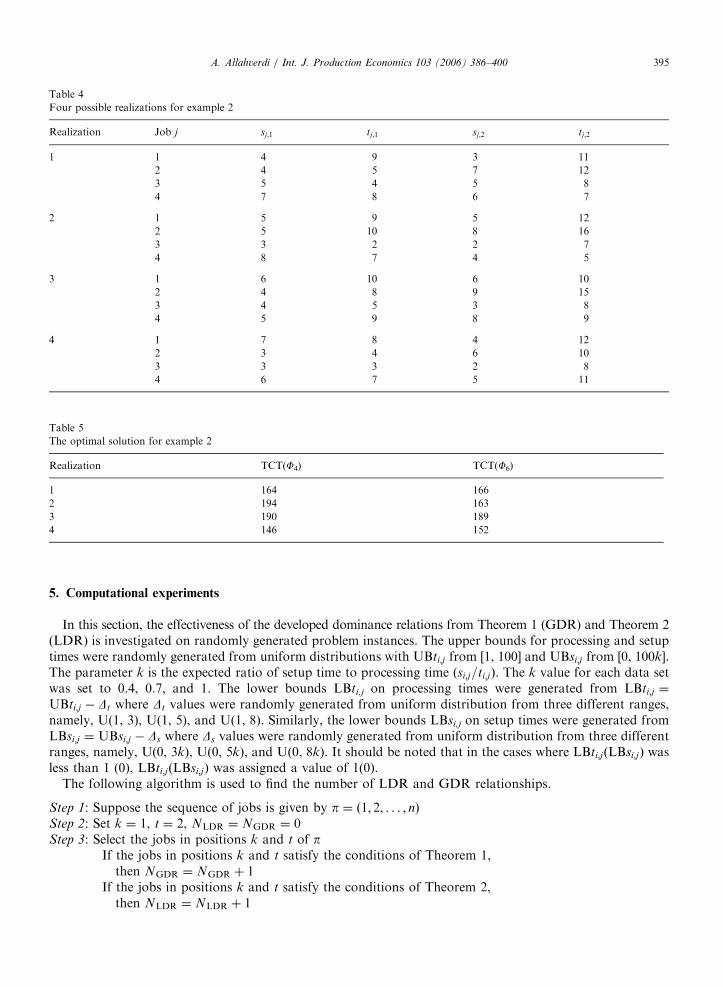
Depending on the realization of setup and processing times, either the sequence F4, or F6, or both will beoptimal. But again we do not know of which of the two sequences F4 and F6 is better until the process is over.Four different realizations of the setup and processing times of the problem described in Table 3 are given inTable 4. The objective function values of both sequences for all the four realizations of Table 4 are given inTable 5. It is clear that the sequence F4 is better for the realizations 1 and 4 while the sequence F6 is better (theoptimal solution) for realizations 2 and 3.

Table 3

Bounds for setup and processing times of example 2

Job j LBsj;1 UBsj:1 LBsj;2 UBsj;2 LBtj;1 UBtj;1 LBtj;2 UBtj;2

1 4 7 2 7 8 12 10 16

2 2 5 6 9 4 10 10 18

3 3 5 2 8 2 6 7 9

4 5 9 4 10 7 9 5 11

ARTICLE IN PRESS

Table 5

The optimal solution for example 2

Realization TCT(F4) TCT(F6)

1 164 166

2 194 163

3 190 189

4 146 152

Table 4

Four possible realizations for example 2

Realization Job j sj;1 tj;1 sj;2 tj;2

1 1 4 9 3 11

2 4 5 7 12

3 5 4 5 8

4 7 8 6 7

2 1 5 9 5 12

2 5 10 8 16

3 3 2 2 7

4 8 7 4 5

3 1 6 10 6 10

2 4 8 9 15

3 4 5 3 8

4 5 9 8 9

4 1 7 8 4 12

2 3 4 6 10

3 3 3 2 8

4 6 7 5 11

A. Allahverdi / Int. J. Production Economics 103 (2006) 386–400 395

5. Computational experiments

In this section, the effectiveness of the developed dominance relations from Theorem 1 (GDR) and Theorem 2(LDR) is investigated on randomly generated problem instances. The upper bounds for processing and setuptimes were randomly generated from uniform distributions with UBti;j from [1, 100] and UBsi;j from [0, 100k].The parameter k is the expected ratio of setup time to processing time ðsi;j=ti;jÞ. The k value for each data setwas set to 0.4, 0.7, and 1. The lower bounds LBti,j on processing times were generated from LBti;j ¼

UBti;j � Dt where Dt values were randomly generated from uniform distribution from three different ranges,namely, U(1, 3), U(1, 5), and U(1, 8). Similarly, the lower bounds LBsi,j on setup times were generated fromLBsi;j ¼ UBsi;j � Ds where Ds values were randomly generated from uniform distribution from three differentranges, namely, U(0, 3k), U(0, 5k), and U(0, 8k). It should be noted that in the cases where LBti;jðLBsi;jÞ wasless than 1 (0), LBti;jðLBsi;jÞ was assigned a value of 1(0).

The following algorithm is used to find the number of LDR and GDR relationships.

Step 1: Suppose the sequence of jobs is given by p ¼ ð1; 2; . . . ; nÞStep 2: Set k ¼ 1, t ¼ 2, NLDR ¼ NGDR ¼ 0Step 3: Select the jobs in positions k and t of p

If the jobs in positions k and t satisfy the conditions of Theorem 1,then NGDR ¼ NGDR þ 1

If the jobs in positions k and t satisfy the conditions of Theorem 2,then NLDR ¼ NLDR þ 1

ARTICLE IN PRESS

Table 6

Computational results for k ¼ 0:4

n Dt Ds LDR GDR

Avg Min Max Avg Min Max

40 U(1,3) U(0,3k) 82.73 28 134 12.00 5 23

40 U(1,3) U(0,5k) 91.13 47 184 11.77 3 33

40 U(1,3) U(0,8k) 77.83 23 134 8.77 2 24

40 U(1,5) U(0,3k) 77.73 25 122 10.43 2 24

40 U(1,5) U(0,5k) 85.27 33 142 9.23 3 15

40 U(1,5) U(0,8k) 71.27 40 118 7.63 1 31

40 U(1,8) U(0,3k) 70.10 32 141 7.17 1 16

40 U(1,8) U(0,5k) 68.27 32 126 7.67 1 22

40 U(1,8) U(0,8k) 63.67 16 109 5.10 0 10

60 U(1,3) U(0,3k) 191.47 96 366 25.40 10 43

60 U(1,3) U(0,5k) 184.07 98 281 25.07 10 39

60 U(1,3) U(0,8k) 183.10 97 308 23.40 11 46

60 U(1,5) U(0,3k) 183.33 105 279 20.77 11 35

60 U(1,5) U(0,5k) 171.63 74 244 21.20 9 33

60 U(1,5) U(0,8k) 155.57 40 259 18.97 9 30

60 U(1,8) U(0,3k) 159.17 71 315 17.00 3 37

60 U(1,8) U(0,5k) 161.03 72 246 14.83 7 29

60 U(1,8) U(0,8k) 143.47 86 234 14.33 5 48

80 U(1,3) U(0,3k) 335.63 191 484 47.27 20 82

80 U(1,3) U(0,5k) 338.97 212 512 51.10 22 75

80 U(1,3) U(0,8k) 309.97 174 480 44.53 21 71

80 U(1,5) U(0,3k) 341.63 202 512 40.20 11 67

80 U(1,5) U(0,5k) 319.20 186 493 38.50 21 68

80 U(1,5) U(0,8k) 292.50 168 453 33.80 17 53

80 U(1,8) U(0,3k) 288.97 146 512 27.57 9 59

80 U(1,8) U(0,5k) 291.10 129 425 24.80 10 46

80 U(1,8) U(0,8k) 267.00 156 373 25.83 6 47

100 U(1,3) U(0,3k) 536.70 264 905 72.50 39 116

100 U(1,3) U(0,5k) 528.60 307 716 75.50 35 105

100 U(1,3) U(0,8k) 508.73 333 695 63.63 33 123

100 U(1,5) U(0,3k) 496.17 364 761 63.17 36 125

100 U(1,5) U(0,5k) 449.33 311 671 57.97 44 76

100 U(1,5) U(0,8k) 460.63 259 678 51.43 28 77

100 U(1,8) U(0,3k) 445.63 259 656 42.50 20 75

100 U(1,8) U(0,5k) 438.37 270 613 41.07 13 68

100 U(1,8) U(0,8k) 427.50 243 617 38.30 11 71

120 U(1,3) U(0,3k) 824.47 533 1256 109.10 67 164

120 U(1,3) U(0,5k) 788.47 516 1152 110.43 77 178

120 U(1,3) U(0,8k) 728.70 490 1021 94.13 58 130

120 U(1,5) U(0,3k) 730.53 408 1067 85.17 51 144

120 U(1,5) U(0,5k) 746.93 503 1066 85.23 52 138

120 U(1,5) U(0,8k) 688.80 448 896 80.30 51 111

120 U(1,8) U(0,3k) 638.57 408 835 60.90 29 115

120 U(1,8) U(0,5k) 643.70 423 1019 58.57 24 99

120 U(1,8) U(0,8k) 590.40 386 887 57.27 26 89

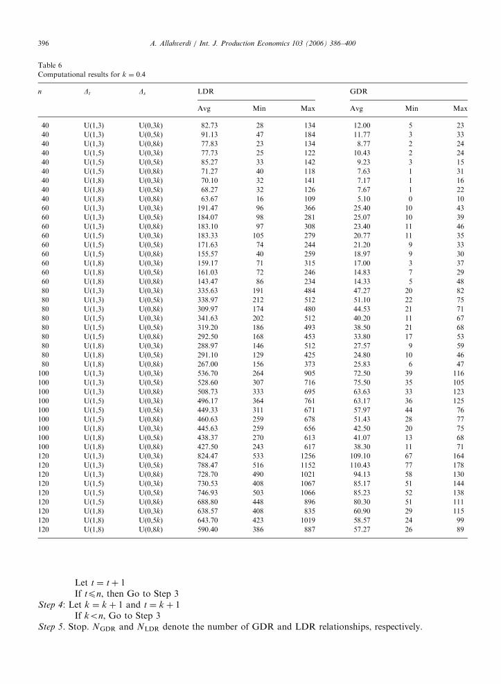
A. Allahverdi / Int. J. Production Economics 103 (2006) 386–400396

Let t ¼ tþ 1If tpn, then Go to Step 3

Step 4: Let k ¼ k þ 1 and t ¼ k þ 1If kon, Go to Step 3

Step 5. Stop. NGDR and NLDR denote the number of GDR and LDR relationships, respectively.

ARTICLE IN PRESS

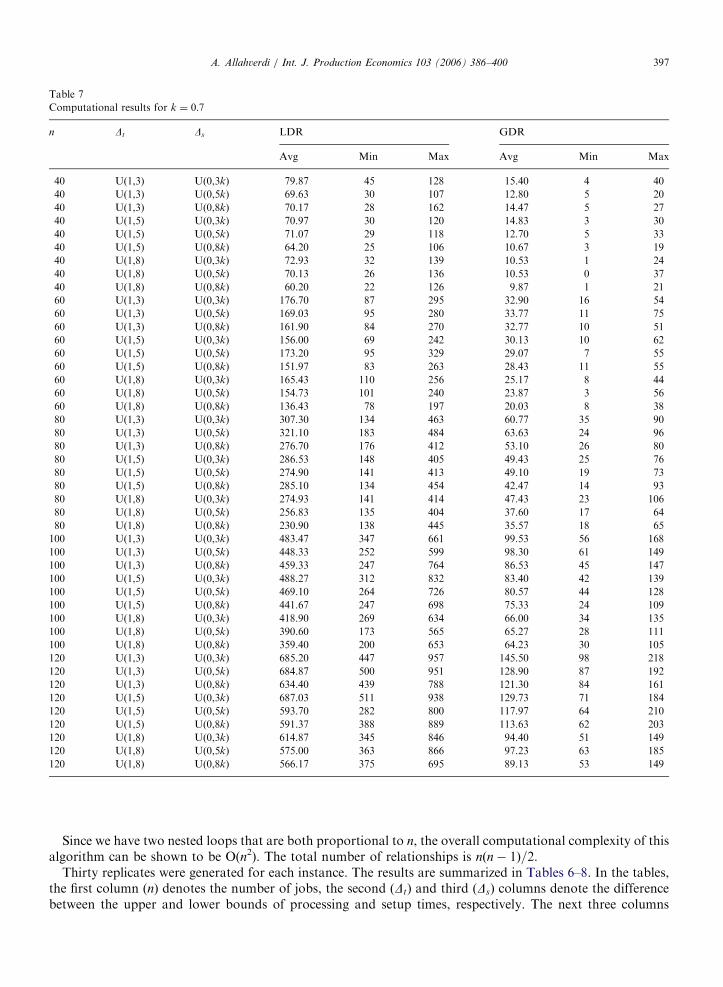
Table 7

Computational results for k ¼ 0:7

n Dt Ds LDR GDR


40 U(1,3) U(0,3k) 79.87 45 128 15.40 4 40

40 U(1,3) U(0,5k) 69.63 30 107 12.80 5 20

40 U(1,3) U(0,8k) 70.17 28 162 14.47 5 27

40 U(1,5) U(0,3k) 70.97 30 120 14.83 3 30

40 U(1,5) U(0,5k) 71.07 29 118 12.70 5 33

40 U(1,5) U(0,8k) 64.20 25 106 10.67 3 19

40 U(1,8) U(0,3k) 72.93 32 139 10.53 1 24

40 U(1,8) U(0,5k) 70.13 26 136 10.53 0 37

40 U(1,8) U(0,8k) 60.20 22 126 9.87 1 21

60 U(1,3) U(0,3k) 176.70 87 295 32.90 16 54

60 U(1,3) U(0,5k) 169.03 95 280 33.77 11 75

60 U(1,3) U(0,8k) 161.90 84 270 32.77 10 51

60 U(1,5) U(0,3k) 156.00 69 242 30.13 10 62

60 U(1,5) U(0,5k) 173.20 95 329 29.07 7 55

60 U(1,5) U(0,8k) 151.97 83 263 28.43 11 55

60 U(1,8) U(0,3k) 165.43 110 256 25.17 8 44

60 U(1,8) U(0,5k) 154.73 101 240 23.87 3 56

60 U(1,8) U(0,8k) 136.43 78 197 20.03 8 38

80 U(1,3) U(0,3k) 307.30 134 463 60.77 35 90

80 U(1,3) U(0,5k) 321.10 183 484 63.63 24 96

80 U(1,3) U(0,8k) 276.70 176 412 53.10 26 80

80 U(1,5) U(0,3k) 286.53 148 405 49.43 25 76

80 U(1,5) U(0,5k) 274.90 141 413 49.10 19 73

80 U(1,5) U(0,8k) 285.10 134 454 42.47 14 93

80 U(1,8) U(0,3k) 274.93 141 414 47.43 23 106

80 U(1,8) U(0,5k) 256.83 135 404 37.60 17 64

80 U(1,8) U(0,8k) 230.90 138 445 35.57 18 65

100 U(1,3) U(0,3k) 483.47 347 661 99.53 56 168

100 U(1,3) U(0,5k) 448.33 252 599 98.30 61 149

100 U(1,3) U(0,8k) 459.33 247 764 86.53 45 147

100 U(1,5) U(0,3k) 488.27 312 832 83.40 42 139

100 U(1,5) U(0,5k) 469.10 264 726 80.57 44 128

100 U(1,5) U(0,8k) 441.67 247 698 75.33 24 109

100 U(1,8) U(0,3k) 418.90 269 634 66.00 34 135

100 U(1,8) U(0,5k) 390.60 173 565 65.27 28 111

100 U(1,8) U(0,8k) 359.40 200 653 64.23 30 105

120 U(1,3) U(0,3k) 685.20 447 957 145.50 98 218

120 U(1,3) U(0,5k) 684.87 500 951 128.90 87 192

120 U(1,3) U(0,8k) 634.40 439 788 121.30 84 161

120 U(1,5) U(0,3k) 687.03 511 938 129.73 71 184

120 U(1,5) U(0,5k) 593.70 282 800 117.97 64 210

120 U(1,5) U(0,8k) 591.37 388 889 113.63 62 203

120 U(1,8) U(0,3k) 614.87 345 846 94.40 51 149

120 U(1,8) U(0,5k) 575.00 363 866 97.23 63 185

120 U(1,8) U(0,8k) 566.17 375 695 89.13 53 149


Since we have two nested loops that are both proportional to n, the overall computational complexity of thisalgorithm can be shown to be O(n2). The total number of relationships is nðn� 1Þ=2.

Thirty replicates were generated for each instance. The results are summarized in Tables 6–8. In the tables,the first column (n) denotes the number of jobs, the second (Dt) and third (Ds) columns denote the differencebetween the upper and lower bounds of processing and setup times, respectively. The next three columns

ARTICLE IN PRESS

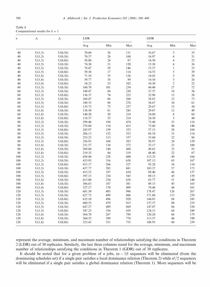
Table 8

Computational results for k ¼ 1

n Dt Ds LDR GDR


40 U(1,3) U(0,3k) 70.60 36 131 16.67 5 35

40 U(1,3) U(0,5k) 70.37 26 160 16.97 6 31

40 U(1,3) U(0,8k) 58.80 24 87 14.50 4 23

40 U(1,5) U(0,3k) 74.30 31 120 15.30 6 36

40 U(1,5) U(0,5k) 78.47 29 146 15.37 1 23

40 U(1,5) U(0,8k) 59.30 17 114 14.53 5 39

40 U(1,8) U(0,3k) 71.10 35 126 14.43 3 29

40 U(1,8) U(0,5k) 59.77 18 89 14.10 5 26

40 U(1,8) U(0,8k) 54.23 25 102 10.30 2 22

60 U(1,3) U(0,3k) 160.70 101 234 44.40 27 72

60 U(1,3) U(0,5k) 149.47 84 230 37.37 18 56

60 U(1,3) U(0,8k) 136.37 74 223 32.90 13 58

60 U(1,5) U(0,3k) 168.47 86 260 38.83 12 73

60 U(1,5) U(0,5k) 149.33 96 276 34.67 10 61

60 U(1,5) U(0,8k) 135.73 75 257 29.67 15 50

60 U(1,8) U(0,3k) 138.50 81 245 29.07 12 49

60 U(1,8) U(0,5k) 140.20 50 219 24.80 8 68

60 U(1,8) U(0,8k) 118.37 55 214 24.30 5 40

80 U(1,3) U(0,3k) 299.40 194 474 73.40 25 118

80 U(1,3) U(0,5k) 278.60 114 415 73.60 40 140

80 U(1,3) U(0,8k) 245.97 159 353 57.13 28 104

80 U(1,5) U(0,3k) 286.13 152 523 68.10 31 114

80 U(1,5) U(0,5k) 253.23 113 337 53.60 22 86

80 U(1,5) U(0,8k) 256.93 104 385 58.97 24 129

80 U(1,8) U(0,3k) 231.57 134 372 52.17 23 100

80 U(1,8) U(0,5k) 269.60 140 480 49.63 23 93

80 U(1,8) U(0,8k) 219.33 84 319 48.40 22 87

100 U(1,3) U(0,3k) 458.40 258 600 113.33 49 166

100 U(1,3) U(0,5k) 433.93 316 638 107.13 65 167

100 U(1,3) U(0,8k) 415.17 266 527 95.20 56 154

100 U(1,5) U(0,3k) 437.77 285 681 103.37 57 175

100 U(1,5) U(0,5k) 415.53 197 654 89.40 46 157

100 U(1,5) U(0,8k) 397.13 234 543 89.13 45 159

100 U(1,8) U(0,3k) 413.00 254 658 83.77 51 140

100 U(1,8) U(0,5k) 386.63 187 581 89.13 45 165

100 U(1,8) U(0,8k) 327.17 170 499 74.40 44 101

120 U(1,3) U(0,3k) 681.30 405 996 178.47 126 267

120 U(1,3) U(0,5k) 627.73 499 806 171.80 113 239

120 U(1,3) U(0,8k) 635.10 496 920 144.83 88 245

120 U(1,5) U(0,3k) 680.53 479 915 157.37 90 235

120 U(1,5) U(0,5k) 647.27 489 869 147.07 86 230

120 U(1,5) U(0,8k) 547.23 336 829 124.13 68 249

120 U(1,8) U(0,3k) 564.70 267 789 120.20 66 179

120 U(1,8) U(0,5k) 564.53 399 776 113.57 46 190

120 U(1,8) U(0,8k) 523.43 331 753 108.93 60 239

A. Allahverdi / Int. J. Production Economics 103 (2006) 386–400398

represent the average, minimum, and maximum number of relationships satisfying the conditions in Theorem2 (LDR) out of 30 replicates. Similarly, the last three columns stand for the average, minimum, and maximumnumber of relationships satisfying the conditions in Theorem 1 (GDR) out of 30 replicates.

It should be noted that for a given problem of n jobs, (n� 1)! sequences will be eliminated (from thedominating schedules set) if a single pair satisfies a local dominance relation (Theorem 2) while n!=2 sequenceswill be eliminated if a single pair satisfies a global dominance relation (Theorem 1). More sequences will be

ARTICLE IN PRESS

0

2

4

6

8

10

40 60 80 100 120Number of jobs

Avg

.

GDR

LDR

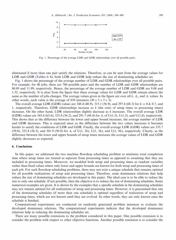
Fig. 1. Percentage of the average LDR and GDR relationships over all possible pairs.


eliminated if more than one pair satisfy the relations. Therefore, as can be seen from the average values forLDR and GDR (Tables 6–8), both LDR and GDR help reduce the size of dominating schedules set.

Fig. 1 shows the percentage of the average number of LDR and GDR relationships over all possible pairs.For example, for 40 jobs, there are 780 possible pairs and the number of LDR and GDR relationships are80.89 and 11.99, respectively. Hence, the percentage of the average number of LDR and GDR are 9.08 and1.52, respectively. It is clear from the figure that these average values for LDR and GDR remain almost thesame as the number of jobs changes. The average values given in the figure are over all k, Ds, and Dt values. Inother words, each value is the average of 810 instances (30� 3� 3� 3).

The overall average LDR (GDR) values are 348.4 (40.9), 315.1 (56.9), and 297.6 (68.3) for k ¼ 0:4, 0.7, and1, respectively. Therefore, GDR relationships increase as k (the ratio of setup times to processing times)increases. On the other hand, LDR relationships slightly decrease as k increases. The overall average LDR(GDR) values are 343.6 (65.6), 325.8 (56.2), and 291.7 (44.4) for Dt of U(1,3), U(1,5), and U(1,8), respectively.This shows that as the difference between the lower and upper bound increases, the average number of LDRand GDR decreases. This is expected since as the difference between the two values increases it becomesharder to satisfy the conditions of LDR and GDR. Finally, the overall average LDR (GDR) values are 335.7(59.0), 323.4 (56.3), and 301.9 (50.9) for Ds of U(1, 3k), U(1, 5k), and U(1, 8k), respectively. Clearly, as thedifference between the lower and upper bounds of setup times increases the average values of LDR and GDRslightly decreases as expected.

6. Conclusions

In this paper, we addressed the two machine flowshop scheduling problem to minimize total completiontime where setup times are treated as separate from processing times as apposed to assuming that they areincluded in processing times. Moreover, we modeled both setup and processing times as random variablesrather than fixed values where only lower and upper bounds are known for both setup and processing times ofeach job. For such flowshop scheduling problems, there may not exist a unique schedule that remains optimalfor all possible realizations of setup and processing times. Therefore, some dominance relations that helpreduce the size of dominating schedules are developed in this paper. The ideal case is to be able to reduce thesize to only one schedule. If not possible, then the objective is to reduce the size of dominating schedules. Somenumerical examples are given. It is shown by the examples that a specific schedule in the dominating schedulesmay not remain optimal for all realizations of setup and processing times. However, it is guaranteed that oneof the dominating schedules (if more than one schedule) is optimal regardless of realization of setup andprocessing times, which are not known until they are evolved. In other words, they are only known once theschedule is finished.

Computational experiments are conducted on randomly generated problem instances to evaluate thedeveloped dominance relations. The computational experiments indicate that the developed dominancerelations help in reducing the dominating schedules set.

There are many possible extensions to the problem considered in this paper. One possible extension is toconsider the problem with respect to other objective functions. Another possible extension is to consider the


same problem with the same objective function but with larger number of machines (m42). Yet anotherpossible extension it to study sequence-dependent random and bounded setup times problem, which is morecomplicated.

There has been some work on parallel machine scheduling problem to minimize makespan where it isassumed that processing times are unknown (only lower and upper bounds are known) and where setup timesare ignored. For example, Angelelli et al. (2003), He and Zhang (1999), and He and Jiang (2004) consideredthe case of two parallel machines and proposed some approximate algorithms for the problem. The design andanalysis of similar approximate algorithm for the problem considered in this paper is another interesting topicto be examined.

Acknowledgements

This research was supported by Kuwait University Research Administration (project EI01/03). The authorwould like to thank two anonymous referees for their useful and constructive comments and suggestions.

References

Allahverdi, A., 2000. Minimizing mean flowtime in a two-machine flowshop with sequence independent setup times. Computers and

Operations Research 27, 111–127.

Allahverdi, A., Aldowaisan, T., Sotskov, Y.N., 2003. Two-machine flowshop scheduling problem to minimize makespan or total

completion time with random and bounded setup times. International Journal of Mathematics and Mathematical Sciences 39,

2475–2486.

Allahverdi, A., Gupta, J.N.D., Aldowiasan, T., 1999. A review of scheduling research involving setup considerations. OMEGA The

International Journal of Management Sciences 27, 219–239.

Allahverdi, A., Sotskov, Y.N., 2003. Two-machine flowshop minimum length scheduling problem with random and bounded processing

times. International Transactions in Operational Research 10, 65–76.

Angelelli, E., Speranza, M.G., Tuza, Z., 2003. Semi-on-line scheduling on two parallel processors with an upper bound on the items.

Algorithmica 37, 243–262.

Bagga, P.C., Khurana, K., 1986. Two-machine flowshop with separated sequence-independent setup times: mean completion time

criterion. Indian Journal of Management and Systems 2, 47–57.

Gonzalez, T., Sahni, S., 1978. Flow shop and job shop schedules. Operations Research 26, 36–52.

He, Y., Jiang, Y., 2004. Optimal algorithms for semi-online preemptive scheduling problems on two uniform machines. Acta Informatica

40, 367–383.

He, Y., Zhang, G., 1999. Semi on-line scheduling on two identical machines. Computing 62, 179–187.

Lai, T.C., Sotskov, Y.N., 1999. Sequencing with uncertain numerical data for makespan minimization. Journal of the Operational

Research Society 50, 230–243.

Lai, T.C., Sotskov, Y.N., Sotskova, N.Y., Werner, F., 1997. Optimal makespan scheduling with given bounds of processing times.

Mathematical and Computer Modelling 26, 67–86.

Logendran, R., Carson, S., Hanson, E., 2005. Group scheduling in flexible flow shops. International Journal of Production Economics 96,

143–155.

Sotskov, Y.N., Allahverdi, A., Lai, T.C., 2004. Flowshop scheduling problem to minimize total completion time with random and

bounded processing times. Journal of Operational Research Society 55, 277–286.

Tang, L., Huang, L., 2005. Optimal and near-optimal algorithms to rolling batch scheduling for seamless steel tube production.

International Journal of Production Economics, in press, doi:10.1016/j.ijpe.2004.04.011.

Yoshida, T., Hitomi, K., 1979. Optimal two-stage production scheduling with set-up times separated. AIIE Transactions 11, 261–263.

dx.doi.org/10.1016/ij.ype.2004.04.011

Documents

Two-machine flowshop scheduling problem to minimize total completion time with bounded setup and processing times