Computers & Operations Research 40 (2013) 1420–1434

Contents lists available at SciVerse ScienceDirect

Computers & Operations Research

0305-05

http://d

n Corr

E-m

journal homepage: www.elsevier.com/locate/caor

Two-machine robotic cell scheduling problem with sequence-dependent setup times

M.H. Fazel Zarandi n, H. Mosadegh, M. Fattahi

Department of Industrial Engineering & Management Systems, Amirkabir University of Technology, 424 Hafez Avenue, 1591634311, Tehran, Iran

a r t i c l e i n f o

Available online 2 October 2012

Keywords:

Robotic cell scheduling

Sequence-dependent setup times

Mixed-integer linear programming

Simulated annealing

Branch and bound

Taguchi

48/$ - see front matter & 2012 Elsevier Ltd. A

x.doi.org/10.1016/j.cor.2012.09.006

esponding author. Tel.: þ98 21 64545378; fa

ail address: zarandi@aut.ac.ir (M.H. Fazel Zar

a b s t r a c t

In this paper, we introduce a new and practical two-machine robotic cell scheduling problem with

sequence-dependent setup times (2RCSDST) along with different loading/unloading times for each part.

Our objective is to simultaneously determine the sequence of robot moves and the sequence of parts

that minimize the total cycle time. The proposed problem is proven to be strongly NP-hard. Using the

Gilmore and Gomory (GnG) algorithm, a polynomial-time computable lower bound is provided.

Based on the input parameters, a dominance condition is developed to determine the optimal

sequence of robot moves for a given sequence of parts. A mixed-integer linear programming (MILP)

model is provided and enhanced using a valid inequality based on the given dominance condition. In

addition, a branch and bound (BnB) algorithm is exploited to solve the problem, and due to the NP-

hardness, an improved simulated annealing (SA) algorithm is proposed to address large-sized test

problems.

All the solution methods are evaluated using small-, medium- and large-sized test problems. The

numerical results indicate that the optimal solution of the MILP model is attained for the medium- and

some large-sized test problems, and the proposed SA, tuned using the Taguchi technique, provides an

acceptable, near-optimal solution with markedly reduced CPU time. Moreover, the lower bound is

observed to be significantly near the optimal solution. Thus, this lower bound is exploited to validate

the results of the SA algorithm for large-sized test problems.

& 2012 Elsevier Ltd. All rights reserved.

1. Introduction

Today, the application of robots in manufacturing systems andin cyclic production strategy is increasingly becoming an inter-esting area of research. Robots can work in various fields such asspot welding, handling, assembling and operations [1]. In thispaper, as in almost all previous studies, the handling robot ismainly considered. Robotic cells consist of one input device, aseries of machines, one output device and robots that handle theparts between the stations [1]. There is no buffer storage betweenmachines, such that each part is being processed or blocked on amachine or being handled by the robot [2]. The objective is tosimultaneously determine the optimal sequence of robot movesand the sequence of parts in a one-unit cyclic problem tominimize the long-run average cycle time or equivalently, tomaximize the throughput [3].

ll rights reserved.

x: þ98 21 66413025.

andi).

1.1. Aims and contributions

The aim of this paper is to introduce a new practical case of thetwo-machine robotic cell scheduling problem and to presentefficient solution methods. As the quantity and variety of pro-ducts increase, setup times, particularly those depending onprevious settings, increasingly influence cell performance. Thisfact raises the need for consideration of sequence-dependentsetup times (SDST) in robotic cell scheduling.

The issue of setup times in a robotic cell is different from setuptimes in traditional scheduling. Without loss of generality, theSDST consists of two sets of activities, i.e., the setup and setdownoperations that are required for each job. A robotic cell also needsthese activities, denoted as loading and unloading operations,before and after each processing. Therefore, this paper focuses onSDST in robotic cells, particularly when loading times are natu-rally defined as sequence-dependent operations. Later, the con-cept and relevance of SDST in robotic cells will be provided withmore details. The contributions of this paper are summarized asfollows:

�

A new two-machine robotic cell scheduling problem of one-unit cycle with sequence-dependent setup times (2RCSDST) is

Nomenclature

P1,P2,...,Pkpart types that must be manufacturedr1,r2,...,rk minimum ratio of parts (in one MPS, rk units of type k

are produced)n¼r1þ?þrk total number of finished parts in the MPS (size

of the MPS)M1, M2 machinesaj processing time of part j on machine M1

bj processing time of part j on machine M2

I, O input and output hoppers, respectivelye0

j grasping time of part j at the input hopper (I)

em1ij loading time of part j on the mth machine after part i,

where m¼1,2em2

j unloading time of part j from the mth machine, wherem¼1,2

e3j dropping time of part j at the output hopper (O)

d traveling time of the robot between I and M1, M1 andM2, M2 and O

2d traveling time of the robot between M2 and I, O andM1

3d traveling time of the robot between O and I

wmi waiting time of the robot before unloading part i from

the mth machine

M.H. Fazel Zarandi et al. / Computers & Operations Research 40 (2013) 1420–1434 1421

introduced. This paper proves that the problem is NP-hard inthe strong sense.

� Using the Gilmore and Gomory (GnG) algorithm, a lower

bound with time complexity of O(n2) for the aforementionedproblem is developed. The lower bound is used for a branchand bound (BnB) algorithm. In addition, the lower bound isused to verify the performance of simulated annealing (SA),another solution method. The SA algorithm is proposedbecause due to intractability, the optimal solutions of large-sized test problems are not provided in a reasonable time.

� A novel mixed-integer linear programming (MILP) model,

simultaneously addressing the problems of determining thebest sequence of robot moves and the best sequence of parts,is developed.

� A valid inequality is developed based on the dominance

condition to enhance the MILP model. Utilizing CPLEX as acommercial solver for solving MILP models, the medium- andsome large-sized test problems can be solved in a reasonabletime. SA is also enhanced by the inclusion of the dominancecondition as well as a well-tuning scheme obtained using theTaguchi technique.

Three newly generated sets of data are used to evaluate theproposed solution methods, the lower bound and the MILP modelby solving a wide range of test problems with different sizes. Thenumerical results indicate the appropriate closeness of the lowerbound to the optimal solution. Furthermore, the solution of theproposed SA is suitably close to the optimal solution, whichconfirms its usefulness in solving larger test problems.

The remainder of the paper is organized as follows. Thefollowing sub-sections review the existing literature and demon-strate how the idea originates. In Section 2, the problem defini-tions, notations and formulations are presented. Section3 presents the lower bound and proves its accuracy. The proposedsolution methods are described in Section 4. Section 5 presentsthe numerical experiments, and Section 6 concludes the paper.

1.2. Literature review

The most recent comprehensive survey and classification ofrobotic problems belong to Dawande et al. [1]. According to theirclassification scheme, the problem discussed in this paper isrepresented as RF29(free, A, MP, cyclic-1)9m, which means two-machine simple robotic cells with one single-gripper robot, freepickup criterion, additive travel-time metric, multiple part-types,producing one unit per cycle and aiming to maximize thethroughput. Bagchi et al. [4] have also presented a detailed reviewof robotic flowshops from the traveling salesman problem (TSP)point of view. The remaining two substantial surveys in this area

discuss cyclic scheduling problems in robotic flowshops [5] andidentical part production in robotic cells [6].

Despite the aforementioned studies, there is still the need foran up-to-date survey including the most recent studies. Thispaper attempts to briefly classify the related works in Table 1.The classification criteria, mainly obtained from [1], are repre-sented as the number of machines (M), single part type (SP),multiple part types (MP), units per cycle (U/C), robot movessequence problem (RMS), parts sequence problem (PS) and themain contributions.

Studies addressing robotic problems are more extensive thanthose listed in Table 1; however, other studies, such as thoseconducted by Suarez and Rosell [31], Soukhal and Martineau [32],Alcaide et al. [33], Brucker and Kampmeyer [34], Yoosefelahi et al.[35] and Levner et al. [36], use different criteria, productionstrategies, number of robots, cell layouts, types of machines andtypes of robot applications than those used in this paper and thepapers discussed in Table 1. For related applications of TSP to thiswork, the reader is referred to Bagchi et al. [4], Deineko et al. [37],Zahrouni and Kamoun [29] and Laporte et al. [38].

1.3. The necessity of 2RCSDST in theory and practice

There has been increasing attention provided to schedulingproblems with setup time considerations. Allahverdi et al. [39]present a survey and classification of scheduling problems withsequence-dependent and sequence-independent setup times(costs). Gupta and Darrow [40], Logendran et al. [41], Liao andJuan [42] and Salmasi and Logendran [43] also consider sequence-dependent setup times. Despite the importance of SDST, to the bestof the authors’ knowledge, no study has addressed the robotic cellscheduling problem with sequence-dependent setup times.

In addition, in the real environment, the modern technology ofa single-gripper robot with higher degrees of freedom may lead tosequence dependencies in peaking up and releasing down objectactivities. A comprehensive, up-to-date study of robot gripperswas conducted by Monkman et al. [44]. Modern grippers usuallyutilize vision-guided grasping systems such as the cameras andsensors used for image processing and visual serving technologies(see [45,46]). When the manufacturing parts differ in sizes anddimensions, the required time for image recognition, jaw settingof the gripper, grasping and unloading the part will also change.

However, when the robot is going to load an object, it takessome time to recognize the position and dimension of the fixture,turn the held part if needed, load the part on the machine, waitfor any necessary adjustments and settings on the part and finallyrelease the object. The importance of time savings in loadingobjects becomes more apparent when computer numerical con-trol (CNC) machines are present in the cell executing multioperations such as welding, drilling, cutting and punching.

Table 1Classification of related papers according to the number of machines (M), single part type (SP), multiple part types (MP), units per cycle (U/C), robot moves sequence

problem (RMS), parts sequence problem (PS) and the main contributions.

Researcher(s) M SP MP U/C RMS PS Main contributions

Sethi et al. [7] 2, 3 | | 1 Given | Application of GnG

Logendran and

Sriskandarajah [8]

2 | | 1 | | 1. Introduction of three robotic cell layouts

2. Application of GnG

Hall et al. [9] 2, 3 | | 1, 2 | | 1. An O(n4) algorithm for a 2-machine cell

2. Calculation of cycle times

Crama and van de

Klundert [10]

m | – 1 | – A dynamic programming approach using O(m3) time complexity

Chen et al. [11] 3, m – | 1 Given | A BnB algorithm

Hall et al. [2] 3 | | 1 | | NP-completeness of RMSs

Sriskandarajah et al. [12] m | | 1 | | 1. Categorization of PSs into 4 groups

2. 2 m-2 of m! potential RMSs are solvable in polynomial time

Aneja and Kamoun [3] 2 – | 1 | | An O(n log n) algorithm

Agnetis [13] 2, 3 – | 1, 2 | | 1. An O(n log n) algorithm for the 2-machine case

2. For a 3-machine case, the optimal cycle is either a 1- or 2-unit cycle

Brauner and Finke [14] 2, 3, 4,

m

| – 1, 2, 3,

k

| – Presentation of an algebraic approach and examination of the validity of an open

conjecture of approximately 1- and 2-unit cycles

Brauner et al. [15] m | – 1 | – 1. Proof that problems with general and symmetric travel times are NP-hard

2. Proof that problems with additive and regular balanced travel times are

solvable in O(m3) and O(1), respectively

Geismar et al. [16] m | – k | – Consideration of parallel machines

Neil Geismar et al. [17] m | – 1, k | – An O(m) algorithm for three types of travel times: additive, constant and Euclidean

Akturk et al. [18] 2 | – 1, 2 | – Assumption of both machines being capable of performing all operations

Gultekin et al. [19] 2 | – 1, 2 | – 1. Consideration of tooling constraint

2. Determination of optimal allocation of operations

Drobouchevitch et al. [20] m | – 1 | – Consideration of a dual-gripper robot

Gultekin et al. [21] 3 | – 1, 2 | – Consideration of processing times as decision variables

Gultekin et al. [22] 2, m | – k | – 1. A new RMS assuming operational flexibility

2. Consideration of number of machines as a decision variable

Dawande et al. [23] 2, m – | 1 | | Investigation of two models: single-gripper cell with output buffer at each machine and the

bufferless dual-gripper cell

Drobouchevitch et al. [24] m | – 1, k | – Consideration of input/output buffers for each machine

Kats and Levner [25] m | – 2 Given – Proposition of an algorithm with O(m4) time complexity

Yildiz et al. [26] m | – k | – Bi-criteria optimization: minimizing cycle time and manufacturing cost

Kimiagari and Mosadegh

[27]

2 – | 1 | | Consideration of different loading and unloading times

Che et al. [28] m – | 2 | Given 1. Consideration of a multi-robot problem

2. An algorithm for determining the optimal number of robots with O(m7) time complexity

Zahrouni and Kamoun [29] 3 – | 1 given | Formulation of the problem as a Generalized TSP

Yildiz et al. [30] 3, m | – k | – Minimization of two objectives: cycle time and total manufacturing cost

The current paper 2 – | 1 | | Extension of the analysis of robotic flowshops to SDST as a new and more challenging case

M.H. Fazel Zarandi et al. / Computers & Operations Research 40 (2013) 1420–14341422

Therefore, the setup time between two different parts requiringdifferent operations will certainly be different from that of twosimilar parts requiring similar operations.

As a conclusion, the sequence dependencies in a robotic cellare important generalizations worth studying, especially whenthe application of new grippers is becoming more popular inmanufacturing cells.

2. Problem description

In flexible manufacturing systems, families of parts, requiringsimilar operations, are categorized to be manufactured in specia-lized cells using a cyclic production strategy (see [3,7,9]). To fulfillthe demand of the planning period, production is separated into h

short cycles and a new set of parts, namely the minimal part set(MPS), is repeatedly manufactured (h times) to satisfy the totaldemand [2]. Here, h is the greatest common divisor of demands,D1, D2yDK, where K is the number of part types. The contributionof each part type in the MPS (dk) is computed as dk¼Dk/h wherek¼1y K.

As an example, consider three parts A, B and C demanding 300,250 and 100 units, respectively. In this case, h is equal to 50, andthe MPS consists of a total of 13 parts, i.e., 6 parts of A, 5 parts of B

and 2 parts of C. Instead of finding the best sequence(s) between650!/(300!�250!�100!) possible permutations of the originalproblem, investigating only 13!/(6!�5!�2!) possible sequencesof the MPS would be sufficient. To mathematically model theproblem, the numbers should be used instead of the letters. Forthe mentioned example, instead of 6 parts of A, numbers 1–6 areutilized. Equivalently, numbers 7–11are used for model B andnumbers 12 and 13 represent model C with the same parameters.

As a result, MPS¼ figni ¼ 1 is the input information of a problem,

where n¼PK

k ¼ 1 dk, and the problem is to determine the

sequence of robot moves and the sequence of parts (MPSsequence) that minimize the steady state cycle time. In theremainder of this paper, MPS represents the aforementionedinput data and the expression MPS sequence refers to a solution

(one of n!=QK

k ¼ 1ðdk!Þ possible sequences) over MPS.

2.1. Assumptions and notations

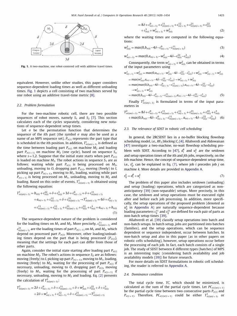
The main assumptions and notations of the problem areborrowed from [3]. The robotic cell contains one robot-centeredcell, two machines, one input device and one output device, andthere is no buffer storage between machines. In most studies, theloading and unloading times for all parts are considered

δ3

M1M2δ

δδ

δ2δ2

Fig. 1. A two-machine, one robot-centered cell with additive travel times.

M.H. Fazel Zarandi et al. / Computers & Operations Research 40 (2013) 1420–1434 1423

equivalent. However, unlike other studies, this paper considerssequence-dependent loading times as well as different unloadingtimes. Fig. 1 depicts a cell consisting of two machines served byone robot using an additive travel-time metric [8].

2.2. Problem formulation

For the two-machine robotic cell, there are two possiblesequences of robot moves, namely S1 and S2 [7]. This sectioncalculates each of the cycles separately, considering new nota-tions of sequence-dependent setup times.

Let s be the permutation function that determines thesequence of the ith part (the symbol s may also be used as aname of an MPS sequence set). Ps(i) represents the part type that

is scheduled in the ith position. In addition, TssðiÞsðiþ1Þ is defined as

the time between loading part Ps(i) on machine M2 and loadingpart Ps(iþ1) on machine M2 (one cycle), based on sequence Ss,where s¼1,2. Suppose that the initial state starts when part Ps(i)

is loaded on machine M2. The robot actions in sequence S1 are asfollows: waiting while part Ps(i) is being processed on M2,unloading, moving to O, dropping part Ps(i), moving (freely) to I,picking up part Ps(iþ1), moving to M1, loading, waiting while partPs(iþ1) is being processed on M1, unloading, moving to M2 and

loading. Based on this order of events, T1sðiÞsðiþ1Þ is obtained using

the following equation:

T1sðiÞsðiþ1Þ ¼ bsðiÞ þe22

sðiÞ þdþe3sðiÞ þ3dþe0

sðiþ1Þ þdþe11sðiÞsðiþ1Þ

þasðiþ1Þ þe12sðiþ1Þ þdþe

21sðiÞsðiþ1Þ-T1

sðiÞsðiþ1Þ ¼ 6dþe0sðiþ1Þ

þe11sðiÞsðiþ1Þ þe

12sðiþ1Þ þe

21sðiÞsðiþ1Þ þe

22sðiÞ þe

3sðiÞ þasðiþ1Þ þbsðiÞ

ð1Þ

The sequence-dependent nature of the problem is considered

for the loading times on M1 and M2. More precisely, e11sðiÞsðiþ1Þ and

e21sðiÞsðiþ1Þ are the loading times of part Ps(iþ1) on M1 and M2, which

depend on processed part Ps(i). Moreover, other loading/unload-ing times depend on the part that is being processed (Ps(i)),meaning that the settings for each part can differ from those ofother parts.

Again, consider the initial state starting after loading part Ps(i)

on machine M2. The robot’s actions in sequence S2 are as follows:moving (freely) to I, picking up part Ps(iþ1), moving to M1, loading,moving (freely) to M2, waiting for the processing of part Ps(i) ifnecessary, unloading, moving to O, dropping part Ps(i), moving(freely) to M1, waiting for the processing of part Ps(iþ1) ifnecessary, unloading, moving to M2 and loading. Eq. (2) presents

the calculation of T2sðiÞsðiþ1Þ:

T2sðiÞsðiþ1Þ ¼ 2dþe0

sðiþ1Þ þdþe11sðiÞsðiþ1Þ þdþw2

sðiÞ þe22sðiÞ þdþe

3sðiÞ

þ2dþw1sðiþ1Þ þe

12sðiþ1Þ þdþe

21sðiÞsðiþ1Þ-T2

sðiÞsðiþ1Þ

¼ 8dþe0sðiþ1Þ þe

11sðiÞsðiþ1Þ þe

12sðiþ1Þ þe

21sðiÞsðiþ1Þ þe

22sðiÞ

þe3sðiÞ þw1

sðiþ1Þ þw2sðiÞ ð2Þ

where the waiting times are computed in the following equa-tions:

w2sðiÞ ¼maxf0,bsðiÞ�4d�e0

sðiþ1Þ�e11sðiÞsðiþ1Þg ð3Þ

w1sðiþ1Þ ¼maxf0,asðiþ1Þ�w2

sðiÞ�4d�e22sðiÞ�e

3sðiÞg ð4Þ

Consequently, the term w1sðiþ1Þ þw2

sðiÞ can be obtained in termsof the input parameters using

w1sðiþ1Þ þw2

sðiÞ ¼maxf0,asðiþ1Þ�w2sðiÞ�4d�e22

sðiÞ�e3sðiÞgþw2

sðiÞ-w1sðiþ1Þ þw2

sðiÞ

¼maxfw2sðiÞ,asðiþ1Þ�4d�e22

sðiÞ�e3sðiÞg-w1

sðiþ1Þ þw2sðiÞ

¼maxfmaxf0,bsðiÞ�4d�e0sðiþ1Þ�e

11sðiÞsðiþ1Þg,asðiþ1Þ�4d�e22

sðiÞ�e3sðiÞg

-w1sðiþ1Þ þw2

sðiÞ

¼maxf0,bsðiÞ�4d�e0sðiþ1Þ�e

11sðiÞsðiþ1Þ,asðiþ1Þ�4d�e22

sðiÞ�e3sðiÞg ð5Þ

Finally T2sðiÞsðiþ1Þ is formulated in terms of the input para-

meters in

T2sðiÞsðiþ1Þ ¼ 8dþe0

sðiþ1Þ þe11sðiÞsðiþ1Þ þe

12sðiþ1Þ þe

21sðiÞsðiþ1Þ þe

22sðiÞ þe

3sðiÞ

þmaxf0,bsðiÞ�4d�e0sðiþ1Þ�e

11sðiÞsðiþ1Þ , asðiþ1Þ�4d�e22

sðiÞ�e3sðiÞg ð6Þ

2.3. The relevance of SDST in robotic cell scheduling

In general, the 2RCSDST lies in a no-buffer blocking flowshopscheduling model, i.e., RF29blocking9Ct [4]. Allahverdi and Aldowaisan[47] investigate a two-machine, no-wait flowshop scheduling pro-

blem with SDST. According to [47], dki and uk

j are the setdown

and setup operation times of the ith and jth jobs, respectively, on thekth machine. Hence, the concept of sequence-dependent setup time,

i.e., skij, can be explained in Eq. (7), where job i precedes job j on

machine k. More details are provided in Appendix A.

skij ¼ dk

i þukj ð7Þ

The problem of this paper also includes setdown (unloading)and setup (loading) operations, which are categorized as non-anticipatory [39] (non-separable) setups. More precisely, in thiscase, the setdown and setup operations must be executed rightafter and before each job processing. In addition, more specifi-cally, the setup operations of the proposed problem (denoted asuk

ij in Appendix A) are naturally sequence-dependent becauseloading parameters e11

ij and e21ij are defined for each pair of parts as

non-batch setup times [39].Allahverdi et al. [39] classify setup operations into batch and

non-batch setups. In batch setup, jobs are partitioned into batches(families), and the setup operations, which can be sequencedependent or sequence independent, occur between batches. Innon-batch setup and also in this paper (as in other papers onrobotic cells scheduling), however, setup operations occur beforethe processing of each job. In fact, each batch consists of a singlejob. The study of SDST between K different types (batches) of MPSis an interesting topic (considering batch availability and jobavailability models [39]) for future research.

For more details on SDST formulations in robotic cell schedul-ing, the reader is referred to Appendix A.

2.4. Dominance condition

The total cycle time, TC, which should be minimized, iscalculated as the sum of the partial cycle times. Let PCs(i)s(iþ1)

be the partial cycle time between two consecutive parts Ps(i) andPs(iþ1). Therefore, PCs(i)s(iþ1) could be either T1

sðiÞsðiþ1Þ or

M.H. Fazel Zarandi et al. / Computers & Operations Research 40 (2013) 1420–14341424

T2sðiÞsðiþ1Þ. The formula of TC is given in Eq. (8), where Ps(nþ1) is the

part that begins the cycle, Ps(1).

TC ¼Xn

i ¼ 1

PCsðiÞsðiþ1Þ ð8Þ

If the MPS sequence is provided, the optimal TC will be obtainedby minimizing each of partial cycle times, i.e., TCn

¼min

ðPn

i ¼ 1 PCsðiÞsðiþ1ÞÞ-TCn¼Pn

i ¼ 1 minðPCsðiÞsðiþ1ÞÞ. In this case, theproblem is reduced to TCn

¼Pn

i ¼ 1 minfT1sðiÞsðiþ1Þ,T

2sðiÞsðiþ1Þg, which

is solvable with an O(n) time complexity using the dominancecondition.

Lemma 1. Dominance condition: for the given MPS sequence s,where i¼1,...,n, if as(iþ1)þbs(i)o2d then PCn

sðiÞsðiþ1Þ ¼ T1sðiÞsðiþ1Þ,

otherwise PCn

sðiÞsðiþ1Þ ¼ T2sðiÞsðiþ1Þ.

Proof. Assuming as(iþ1)þbs(i)o2d the term T1sðiÞsðiþ1Þ�T2

sðiÞsðiþ1Þ

is computed as follows:

T1sðiÞsðiþ1Þ�T2

sðiÞsðiþ1Þ ¼ asðiþ1Þ þbsðiÞ�maxf0,bsðiÞ�4d�e0sðiþ1Þ

�e11sðiÞsðiþ1Þ,asðiþ1Þ�4d�e22

sðiÞ�e3sðiÞg�2d

-T1sðiÞsðiþ1Þ�T2

sðiÞsðiþ1Þ ¼minfasðiþ1Þ þbsðiÞ,asðiþ1Þ þ4dþe0sðiþ1Þ

þe11sðiÞsðiþ1Þ,bsðiÞ þ4dþe22

sðiÞ þe3sðiÞg�2d

Because as(iþ1)þbs(i)o2d, T1sðiÞsðiþ1Þ�T2

sðiÞsðiþ1Þ ¼ asðiþ1Þ þbsðiÞ�2d-T1

sðiÞsðiþ1ÞoT2sðiÞsðiþ1Þ.

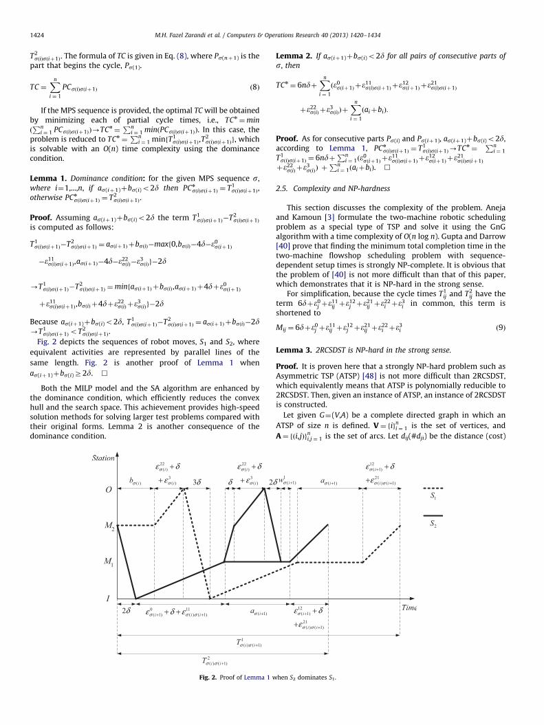
Fig. 2 depicts the sequences of robot moves, S1 and S2, where

equivalent activities are represented by parallel lines of the

same length. Fig. 2 is another proof of Lemma 1 when

as(iþ1)þbs(i)Z2d. &

Both the MILP model and the SA algorithm are enhanced bythe dominance condition, which efficiently reduces the convexhull and the search space. This achievement provides high-speedsolution methods for solving larger test problems compared withtheir original forms. Lemma 2 is another consequence of thedominance condition.

I

1M

2M

O

2δ 0 11( 1) ( ) ( 1)i i iσ σ σε δ ε+ ++ + ( 1)iaσ +

2δδ

22( )

3( )

i

i

σ

σ

ε δ

ε

+

+

22( )

3( )

i

i

σ

σ

ε δ

ε

+

+( )ibσ 3δ

1( ) ( 1)i iTσ σ +

2( ) ( 1)i iTσ σ +

Fig. 2. Proof of Lemma 1 w

Lemma 2. If as(iþ1)þbs(i)o2d for all pairs of consecutive parts of

s, then

TCn¼ 6ndþ

Xn

i ¼ 1

ðe0sðiþ1Þ þe

11sðiÞsðiþ1Þ þe

12sðiþ1Þ þe

21sðiÞsðiþ1Þ

þe22sðiÞ þe

3sðiÞÞþ

Xn

i ¼ 1

ðaiþbiÞ:

Proof. As for consecutive parts Ps(i) and Ps(iþ1), as(iþ1)þbs(i)o2d,according to Lemma 1, PCn

sðiÞsðiþ1Þ ¼ T1sðiÞsðiþ1Þ-TCn

¼Pn

i ¼ 1

T1sðiÞsðiþ1Þ ¼ 6ndþ

Pni ¼ 1ðe0

sðiþ1Þ þe11sðiÞsðiþ1Þ þe

12sðiþ1Þ þe

21sðiÞsðiþ1Þ

þe22sðiÞ þe

3sðiÞÞ þ

Pni ¼ 1ðaiþbiÞ. &

2.5. Complexity and NP-hardness

This section discusses the complexity of the problem. Anejaand Kamoun [3] formulate the two-machine robotic schedulingproblem as a special type of TSP and solve it using the GnGalgorithm with a time complexity of O(n log n). Gupta and Darrow[40] prove that finding the minimum total completion time in thetwo-machine flowshop scheduling problem with sequence-dependent setup times is strongly NP-complete. It is obvious thatthe problem of [40] is not more difficult than that of this paper,which demonstrates that it is NP-hard in the strong sense.

For simplification, because the cycle times T1ij and T2

ij have theterm 6dþe0

j þe11ij þe

12j þe

21ij þe

22i þe

3i in common, this term is

shortened to

Mij ¼ 6dþe0j þe

11ij þe

12j þe

21ij þe

22i þe

3i ð9Þ

Lemma 3. 2RCSDST is NP-hard in the strong sense.

Proof. It is proven here that a strongly NP-hard problem such asAsymmetric TSP (ATSP) [48] is not more difficult than 2RCSDST,which equivalently means that ATSP is polynomially reducible to2RCSDST. Then, given an instance of ATSP, an instance of 2RCSDSTis constructed.

Let given G¼(V,A) be a complete directed graph in which an

ATSP of size n is defined. V¼ figni ¼ 1 is the set of vertices, and

A¼ fði,jÞgni,j ¼ 1 is the set of arcs. Let dij(#dji) be the distance (cost)

12( 1)

21( ) ( 1)

i

i i

σ

σ σ

ε δ

ε+

+

+

+

1( 1)iwσ + ( 1)iaσ +

12( 1)

21( ) ( 1)

i

i i

σ

σ σ

ε δ

ε+

+

+

+

1S

2S

hen S2 dominates S1.

M.H. Fazel Zarandi et al. / Computers & Operations Research 40 (2013) 1420–1434 1425

of arc (i,j)AA, such that 1odijoN, where i#j and dij¼N where

i¼ j for each i,jAV. The objective is to find a Hamiltonian tour

(cyclic permutation of V elements) of G with the shortest possible

length of a closed path, which visits all nodes, each one precisely

once. Based on Lemma 1, the instance of 2RCSDST is constructed

as a case that S1 always dominates S2. The reduction is performed

using the following steps:

�

Set dmin ¼ mini,jA Vfdijg,

�

Set aj¼bj¼0 for each jAV, � Set e0

j ¼ e12j ¼ e

22j ¼ e

3j ¼ 0 for each jAV,

�

Set e11ij ¼ e

21ij ¼ ðdij�dminþ1Þ=2 for each i,jAV,

�

Set d¼ ðdmin�1Þ=6.

Now, let s* be the optimal MPS sequence of the constructed

2RCSDST instance. Because for each i,jAV, dij41, then dmin41

and dmin�140, which implies d40. Furthermore, for each iAV,

asnðiþ1Þ þbsnðiÞ ¼ 0 and asnðiþ1Þ þbsnðiÞo2d. Referring to Lemma 2,

the minimum total cycle time for the given s* is computed as

follows:

TCn¼Xn

i ¼ 1

T1snðiÞsnðiþ1Þ ¼ 6ndþ

Xn

i ¼ 1

ðe11snðiÞsnðiþ1Þ þe

21snðiÞsnðiþ1ÞÞ

-TCn¼ 6n

dmin�1

6

þXiAV

dsnðiÞsnðiþ1Þ�dminþ1

2þ

dsnðiÞsnðiþ1Þ�dminþ1

2

� �-TCn

¼XiAV

dsnðiÞsnðiþ1Þ ð10Þ

Thus, TC* represents the length of an optimal Hamiltonian tour.

Now, it can be stated that s* will solve the ATSP instance if and

only if it can be easily transformed into a solution of the ASTP in G

such as H*CA. The equivalent optimal tour is attainable as

Hn¼ fðsnðiÞ,snðiþ1ÞÞgni ¼ 1, where s*(nþ1)¼s*(1). The reduction

is performed with a time complexity of O(n2). This is a cogent

case to claim that 2RCSDST is strongly NP-hard. &

3. Lower bound

The aim of defining a lower bound is first to solve the problemusing the branch and bound algorithm and second to verify theinexact solution methods, particularly for large-scaled optimiza-tion problems with no available exact solutions.

The idea behind the concept is that the sequence-dependentversion of the problem should be relaxed to a sequence-independent one. For this purpose, the loading times on M1 andM2 are changed to a constant value, i.e., the minimum relevantvalue of each part. In the second phase, the problem is solvedusing the dominance condition and the Gilmore and Gomoryalgorithm. The lower bound is computed using the seven steps ofAlgorithm I.

Algorithm I. Lower bound

Step 1. For each jAMPS, set e11nj ¼ min

n

i ¼ 1fe11

ij g and e21nj ¼ min

n

i ¼ 1fe21

ij g

Step 2. Set m¼ 6ndþPn

j ¼ 1

ðe0j þe

11nj þe

12j þe

21nj þe

22j þe

3j Þ

Step 3. Set z¼ minn

fa gþ minn

fb g

j ¼ 1

jj ¼ 1

j

Step 4. Set p1 ¼ minn

j ¼ 1fajg�3d�max

n

j ¼ 1fe0

j g�maxn

j ¼ 1fe11

nj g and p2 ¼

minn

j ¼ 1fbjg�3d�max

n

j ¼ 1fe22

j g�maxn

j ¼ 1fe3

j g

Step 5. For each jAMPS, set ej¼max{z,ajþp2} and fj¼bjþp1

Step 6. Solve P: MinfCTGnG ¼Pn

k ¼ 1

maxfekþ1,f kgg using the GnG

algorithm

Step 7. Compute the lower bound: LB¼ mþCTn

GnG.

Lemma 4. The lower bound (LB) computed using Algorithm I is less

than or equal to the optimal solution.

Proof. Algorithm I utilizes two main relaxations to reach thelower bound. In the first relaxation, the sequence-dependentproblem, namely P(1), is reduced to the sequence-independent

problem, namely P(2), according to Step 1. Let TCn

Pð1Þand TCn

Pð2Þbe

the optimal total cycle times of P(1) and P(2), respectively. It is

obvious that TCn

Pð2ÞrTCn

Pð1Þ. Then, TCn

Pð2Þshould be determined.

Using the dominance condition, the parameters are manipulatedin a manner that, for all consecutive parts, S2 dominates S1. Themanipulation is concerned about the distance between M2 and I andthe distance between M1 and O, which are represented as ‘ and ‘0,respectively, instead of 2d. The new partial cycle times betweenconsecutive parts i and j are reformulated as Eqs. (11)-(13).

M0ij ¼ 6dþe0j þe

11nj þe

12j þe

21nj þe

22i þe

3i ð11Þ

T 01ij ¼M0ijþajþbi ð12Þ

T 02ij ¼M0ijþmaxf‘þ‘0�2d,biþ‘0�4d�e0

j �e11nj ,ajþ‘�4d�e22

i �e3i g

ð13Þ

The aim is to determine ‘ and ‘0 in a manner that Eq. (14), i.e.,the term T 0ij1�T 0ij2, is always nonnegative for all consecutive partsi and j.

T 01ij �T 02ij ¼minfajþbi�‘�‘0þ2d,aj�‘

0þ4dþe0

j þe11nj ,bi�‘þ4dþe22

i þe3i g

ð14Þ

For this purpose, all terms of the equation should be non-negative, subject to:

ajþbiZ‘þ‘0�2d i¼ 1,2,:::,n; j¼ 1,2,:::,n ð15Þ

ajZ‘0�4d�e0

j �e11nj j¼ 1,2,:::,n ð16Þ

biZ‘�4d�e22i �e

3i i¼ 1,2,:::,n ð17Þ

Constraints (15)–(17) can be summarized as (i)ajZ‘0�d and

(ii) bjZ‘�d. As a result, the greatest possible values of ‘ and ‘0

that satisfy constraints (15)–(17) are formulated as Eqs. (18) and(19).

‘¼ minn

j ¼ 1fbjgþd ð18Þ

‘0 ¼ minn

j ¼ 1fajgþd ð19Þ

Substituting Eqs. (18) and (19) into Eqs. (13) and (14) leads tothe following equations:

T 02ij ¼M0ijþmaxfðminn

j ¼ 1fajgþ min

n

j ¼ 1fbjgÞ,ðbiþ min

n

j ¼ 1fajgÞ�3d�e0

j

�e11nj ,ðajþ min

n

j ¼ 1fbjgÞ�3d�e22

i �e3i g ð20Þ

M.H. Fazel Zarandi et al. / Computers & Operations Research 40 (2013) 1420–14341426

T 01ij �T 0ij2¼minfðaj�minn

j ¼ 1fajgÞþðbj�min

n

j ¼ 1fbjgÞ,ðaj�min

n

j ¼ 1fajgÞþ3dþe0

j

þe11nj ,ðbj�min

n

j ¼ 1fbjgÞþ3dþe22

i þe3i g ð21Þ

Now, it is obvious that the term T 0ij1�T 0ij2 is nonnegative

because: first, minnj ¼ 1fajgraj 8jAMPS and minn

j ¼ 1fbjgr bj8jA

MPS- faj�minnj ¼ 1fajggþðbj�minn

j ¼ 1fbjgÞZ0, second, ðaj�minnj ¼ 1

fajgÞþ3dþe0j þ e11

nj Z0 and third, ðbj�minnj ¼ 1fbjgÞþ 3dþe22

i þ

e3i Z0. The optimal cycle time of P(2) is now obtained by mini-

mizing Eq. (22).

CTPð2Þ ¼X

i,j AMPS

T 0ij2¼X

i,j AMPS

M0ij

þX

i,j AMPS

maxfðminn

j ¼ 1fajgþ min

n

j ¼ 1fbjgÞ,ðbiþ min

n

j ¼ 1fajgÞ

�3d�e0j �e

11nj ,ðajþ min

n

j ¼ 1fbjgÞ�3d�e22

i �e3i g ð22Þ

The first termP

i,jAMPSM0ij

� �is constant and independent from

the sequence of parts. Hence,P

i,jAMPSM0ij ¼Pn

i ¼ 1 6dþPn

j ¼ 1

ðe0j þe

11nj þe12

j þe21nj Þþ

Pni ¼ 1 ðe22

i þe3i Þ-m¼ 6ndþ

Pnj ¼ 1ðe0

j þe11nj

þe12j þe

21nj þe

22j þe

3j Þ. Therefore, the problem is reduced to mini-

mizing the second term, which is very difficult to solve because

some terms of the formulation, i.e., ðbiþminnj ¼ 1fajgÞ�3d�e0

j �e11nj

and ðajþminnj ¼ 1fbjgÞ�3d �e22

i �e3i , depend on the sequence. Here,

the second relaxation is performed by reformulating each of theterms as

z¼ minn

j ¼ 1fajgþ min

n

j ¼ 1fbjg ð23Þ

p1 ¼ minn

j ¼ 1fajg�3d�max

n

j ¼ 1fe0

j g�maxn

j ¼ 1fe11

nj g ð24Þ

p2 ¼ minn

j ¼ 1fbjg�3d�max

n

j ¼ 1fe22

i g�maxn

j ¼ 1fe3

i g ð25Þ

It is obvious that biþp1rðbiþminnj ¼ 1fajgÞ�3d�e0

j �e11nj and

ajþp2r ðajþminnj ¼ 1fbjgÞ�3d�e22

i �e3i 8i, jAMPS. The new pro-

blem, namely P(3), formulated as Eqs. (26)–(28), is now solvableusing the GnG algorithm.

ej ¼maxfz,ajþp2g ð26Þ

f j ¼ bjþp1 ð27Þ

CTGnG ¼Xn

k ¼ 1

maxfekþ1,f kg ð28Þ

Finally, the lower bound is computed asLB¼ mþCTn

GnG.

4. Solution methods

This paper presents some well-known and prominent methodsfor solving the introduced problem. Lemma 3 proves that theproblem is strongly NP-hard. This fact necessitates the use ofefficient algorithms that have good performance from threepoints of view: the solutions’ quality, the CPU time and therequired memory space. One of the algorithms that are utilizedin this paper, the BnB algorithm, provides the exact optimalsolution (OS). However, for large-sized test problems, the CPUtime and the memory space used will significantly increase. Thesedrawbacks are the same as those we encountered when using thedeveloped MILP model, which is solved using CPLEX. However,

the enhanced version of MILP can be used for medium- andsometimes large-sized test problems on computers with higherRAM. Furthermore, a metaheuristic approach, namely SA, can beused and provides a near-optimal solution in a few seconds.

4.1. Mixed-integer linear programming model

Here, a mixed-integer linear programming model is proposedwhich is the first one that simultaneously considers both robot-moves-sequencing and part-sequencing problems. The decisionvariables and parameters of the proposed model are introduced.

4.1.1. Parameters and decision variables

Let n be the size of the MPS with i¼1, 2,y,n; j¼1, 2,y,n.Other parameters are introduced in Eqs. (29)–(32). Mij waspreviously formulated as Eq. (9). Eq. (29) is the robot moves cycletime of consecutive parts i and j under S1.

aij ¼Mijþajþbi 8i, jAMPS, ia j ð29Þ

Another robot moves cycle time, computed in Eq. (6), can bedivided into the three following parts:

b1ij ¼Mijþ2d 8i, jAMPS, ia j ð30Þ

b2ij ¼Mijþbi�2d�e0

j �e11ij 8i, jAMPS, ia j ð31Þ

b3ij ¼Mijþaj�2d�e22

i �e3i 8i, jAMPS, ia j ð32Þ

There are two sets of decision variables, namely x and y,defined as follows: yij: partial cycle time of consecutive parts i andj,8i, jAMPS, ia j

xsij ¼

1 if part j is scheduled immediately af ter part i under the

sequence of robot moves Ss 8i, j AMPS, ia j, s¼ 1, 2

0 otherwise:

8><>:

4.1.2. Basic MILP model

Generally, three types of constraints, namely sequential,demand and cyclic constraints must be considered in the pro-posed model. To specify that only one part must be scheduledafter and before each part in the sequence, constraints (33) and(34) are considered.

Xn

j¼ 1

ja i

X2

s ¼ 1

xsijr1 8iAMPS ð33Þ

Xn

i¼ 1

ia j

X2

s ¼ 1

xsijr1 8jAMPS ð34Þ

Another sequential constraint that prevents rescheduling part i

after part j when it has been scheduled before part j, or vice versa,is formulated as follows:

X2

s ¼ 1

xsijþ

X2

s ¼ 1

xsjir1 8i, jAMPS, io j ð35Þ

Eq. (36) provides the demand constraint, where the totaldemand of MPS (n¼

PkAMPSdk) is satisfied.

Xn

i ¼ 1

Xn

j ¼ 1

X2

s ¼ 1

xsij ¼ n ð36Þ

For the cycle time constraints, first consider T2ij , which includes

a max operator over three terms, i.e., Eqs. (30)–(32). If thesequence of robot moves S2 is selected, then x2

ij ¼ 1 and x1ij ¼ 0.

Consequently, the partial cycle time yij should be greater than or

M.H. Fazel Zarandi et al. / Computers & Operations Research 40 (2013) 1420–1434 1427

equal to all terms as demonstrated by the following constraints:

b1ijx

2ijryij 8i, jAMPS, ia j ð37Þ

b2ijx

2ijryij 8i, jAMPS, ia j ð38Þ

b3ijx

2ijryij 8i, jAMPS, ia j ð39Þ

In the second situation, where x1ij ¼ 1 and x2

ij ¼ 0, the followingconstraint will be active or, equivalently, the partial cycle timewill be equal to T1

ij.

aijx1ijryij 8i, jAMPS, ia j ð40Þ

The final constraint concerns binary variables.

xsij ¼ 0,1 8i, jAMPS, ia j; 8sAf1,2g ð41Þ

The objective function or the total cycle time, given by Eq. (42),is equal to the sum of the partial cycle times, i.e., the yijs.

TC ¼Xn

i ¼ 1

Xn

j ¼ 1

yij ð42Þ

Now, the problem can be represented as PB: Min{TC 9 con-straints (33)–(41)}. The presented model is coded in a GeneralAlgebraic Modeling System (GAMS) 22.2 environment and solvedusing the CPLEX solver.

4.1.3. Enhanced MILP model

Another advantage of the dominance condition (Lemma 1) isthe enhancement of the proposed solution methods. It can beadded to the model as a valid inequality, i.e., constraint (43),which significantly improves the speed and efficiency of thesolution procedure and, hence, makes solving larger test problemspossible

gijx1ijrgijx

2ij 8i, jAMPS, ia j ð43Þ

g is another set of parameters originating from the dominancecondition. Eq. (44) formulates this parameter for all possibleconsecutive parts i and j.

gij ¼ ajþbi�2d 8i, jAMPS, ia j ð44Þ

The problem can be now represented as PE: Min {TC 9 constraints(33)–(41) and (43)} and solved using the CPLEX solver. With respectto the E-MILP model, there are 3� (n2

�n) variables (including binaryvariables) and 11/2n2

�7/2nþ1 constraints (without constraint (41))for a problem of size n.

4.2. Simulated annealing

Although the MILP model guarantees the optimal solution,because of the NP-hardness, even well-known software technol-ogies such as CPLEX cannot solve the large-sized test problems.Bagchi et al. [4] note that in the real world, the size of an MPS canbe larger than 50 parts. In such cases, the robotic cell schedulingproblem can be considered a large scale optimization problem.Using the dominance condition, the search space is reduced toonly investigating different orders of MPS elements, thus makingthe solution procedure more efficient. As a nimble metaheuristicalgorithm, SA appears to be suitable for these types of searchspaces. The application of SA in recent publications (see [49–51])demonstrates its suitability in solving well-known and timelyproblems. Despite new versions of SA [52], this paper focuses onimproving the search process using a simple SA, originated byKirkpatrick [53], as well as controlling and conducting tuningeffects using the Taguchi technique reported in [51,54–56].

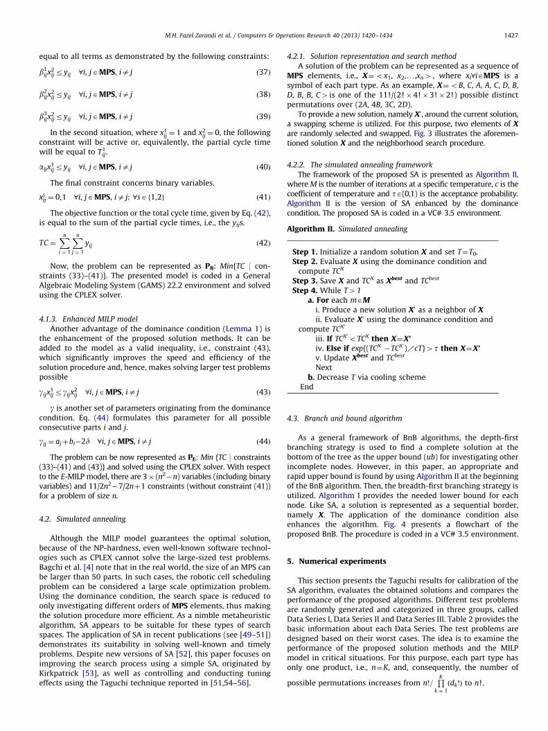
4.2.1. Solution representation and search method

A solution of the problem can be represented as a sequence ofMPS elements, i.e., X¼ox1, x2,y,xn4 , where xi8iAMPS is asymbol of each part type. As an example, X¼oB, C, A, A, C, D, B,D, B, B, C4 is one of the 11!/(2!�4!�3!�2!) possible distinctpermutations over (2A, 4B, 3C, 2D).

To provide a new solution, namely X0, around the current solution,a swapping scheme is utilized. For this purpose, two elements of Xare randomly selected and swapped. Fig. 3 illustrates the aforemen-tioned solution X and the neighborhood search procedure.

4.2.2. The simulated annealing framework

The framework of the proposed SA is presented as Algorithm II,where M is the number of iterations at a specific temperature, c is thecoefficient of temperature and tA(0,1) is the acceptance probability.Algorithm II is the version of SA enhanced by the dominancecondition. The proposed SA is coded in a VC# 3.5 environment.

Algorithm II. Simulated annealing

Step 1. Initialize a random solution X and set T¼T0.Step 2. Evaluate X using the dominance condition and

compute TCX

Step 3. Save X and TCX as Xbest and TCbest

Step 4. While T41

a. For each mAMi. Produce a new solution X0 as a neighbor of Xii. Evaluate X0 using the dominance condition and

compute TCX’

iii. If TCX0oTCX then X¼X’iv. Else if exp{(TCX

�TCX0)XcT}4t then X¼X’v. Update Xbest and TCbest

Nextb. Decrease T via cooling scheme

End

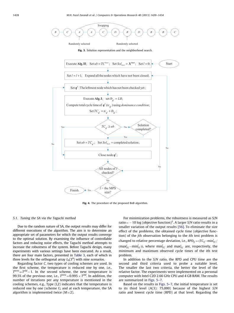
4.3. Branch and bound algorithm

As a general framework of BnB algorithms, the depth-firstbranching strategy is used to find a complete solution at thebottom of the tree as the upper bound (ub) for investigating otherincomplete nodes. However, in this paper, an appropriate andrapid upper bound is found by using Algorithm II at the beginningof the BnB algorithm. Then, the breadth-first branching strategy isutilized. Algorithm I provides the needed lower bound for eachnode. Like SA, a solution is represented as a sequential border,namely X. The application of the dominance condition alsoenhances the algorithm. Fig. 4 presents a flowchart of theproposed BnB. The procedure is coded in a VC# 3.5 environment.

5. Numerical experiments

This section presents the Taguchi results for calibration of theSA algorithm, evaluates the obtained solutions and compares theperformance of the proposed algorithms. Different test problemsare randomly generated and categorized in three groups, calledData Series I, Data Series II and Data Series III. Table 2 provides thebasic information about each Data Series. The test problems aredesigned based on their worst cases. The idea is to examine theperformance of the proposed solution methods and the MILPmodel in critical situations. For this purpose, each part type hasonly one product, i.e., n¼K, and, consequently, the number of

possible permutations increases from n!=QK

k ¼ 1

ðdk!Þ to n!.

C BDBDCAA B

Swapping

Randomly selected Randomly selected

B C

Fig. 3. Solution representation and the neighborhood search.

Fig. 4. The procedure of the proposed BnB algorithm.

M.H. Fazel Zarandi et al. / Computers & Operations Research 40 (2013) 1420–14341428

5.1. Tuning the SA via the Taguchi method

Due to the random nature of SA, the output results may differ fordifferent executions of the algorithm. The aim is to determine anappropriate set of parameters for which the output results convergeto the optimal solution. By examining the influence of controllablefactors and reducing noise effects, the Taguchi method attempts toincrease the robustness of the system. Before Taguchi design, manyexperiments with various settings have been executed. As a result,there are four main factors, presented in Table 3, each of which inthree levels for the orthogonal array L9(34) with nine scenarios.

Regarding factor C, two types of cooling schemes are used. Inthe first scheme, the temperature is reduced one by one, i.e.,Tnew¼Told

�1. In the second scheme, the new temperature is99.5% of the previous one, i.e., Tnew

¼0.995� Told. In addition, thenumber of iterations per any temperature is mentioned in thecooling schemes, e.g., Type (I,2) indicates that the temperature isreduced one by one (scheme I), and at each temperature, the SAalgorithm is implemented twice (M¼2).

For minimization problems, the robustness is measured as S/N

ratio¼�10 log (objective function)2. A larger S/N ratio results in a

smaller variation of the output results [56]. To eliminate the size

effect of the problems, the obtained cycle time (objective func-

tion) of the jth observation belonging to the ith test problem is

changed to relative percentage deviation, i.e., RPDij ¼ ðTCij�miniTC=

ðmaxiTC�mini

TCÞÞ, where miniTC and maxi

TC are, respectively, the

minimum and maximum observed cycle times of the ith test

problem.In addition to the S/N ratio, the RPD and CPU time are the

second and third criteria used to probe a suitable level.The smaller the last two criteria, the better the level of therelative factor. The experiments were implemented on a personalcomputer with Intel C2D 2.66 GHz CPU and 4 GB RAM. The resultsare summarized in Figs. 5–7.

Based on the results in Figs. 5–7, the initial temperature is setto its third level (A(3): 75,000) because of the highest S/Nratio and lowest cycle time (RPD) at that level. Regarding the

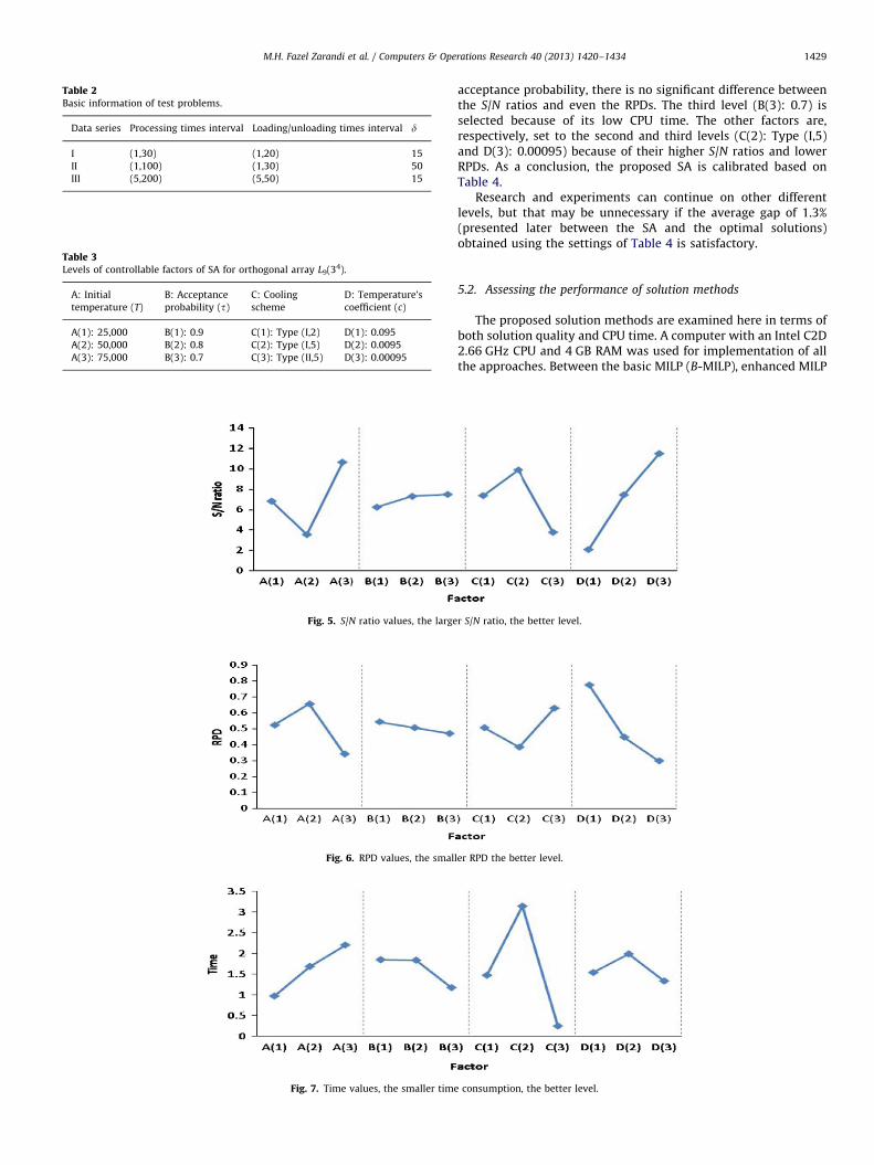
Table 2Basic information of test problems.

Data series Processing times interval Loading/unloading times interval d

I (1,30) (1,20) 15

II (1,100) (1,30) 50

III (5,200) (5,50) 15

Table 3Levels of controllable factors of SA for orthogonal array L9(34).

A: Initial

temperature (T)

B: Acceptance

probability (t)

C: Cooling

scheme

D: Temperature’s

coefficient (c)

A(1): 25,000 B(1): 0.9 C(1): Type (I,2) D(1): 0.095

A(2): 50,000 B(2): 0.8 C(2): Type (I,5) D(2): 0.0095

A(3): 75,000 B(3): 0.7 C(3): Type (II,5) D(3): 0.00095

Fig. 5. S/N ratio values, the large

Fig. 6. RPD values, the smal

Fig. 7. Time values, the smaller time

M.H. Fazel Zarandi et al. / Computers & Operations Research 40 (2013) 1420–1434 1429

acceptance probability, there is no significant difference betweenthe S/N ratios and even the RPDs. The third level (B(3): 0.7) isselected because of its low CPU time. The other factors are,respectively, set to the second and third levels (C(2): Type (I,5)and D(3): 0.00095) because of their higher S/N ratios and lowerRPDs. As a conclusion, the proposed SA is calibrated based onTable 4.

Research and experiments can continue on other differentlevels, but that may be unnecessary if the average gap of 1.3%(presented later between the SA and the optimal solutions)obtained using the settings of Table 4 is satisfactory.

5.2. Assessing the performance of solution methods

The proposed solution methods are examined here in terms ofboth solution quality and CPU time. A computer with an Intel C2D2.66 GHz CPU and 4 GB RAM was used for implementation of allthe approaches. Between the basic MILP (B-MILP), enhanced MILP

r S/N ratio, the better level.

ler RPD the better level.

consumption, the better level.

M.H. Fazel Zarandi et al. / Computers & Operations Research 40 (2013) 1420–14341430

(E-MILP), BnB and SA, BnB performed the worst. It was able toonly solve test problems with no more than 11 parts in areasonable time. As computational results show, CPLEX can solveproblems with 175 parts and hence the BnB results are not muchconsiderable to be discussed.

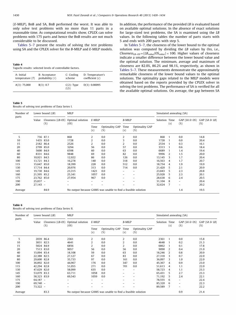
Tables 5–7 present the results of solving the test problemsusing SA and the CPLEX solver for the B-MILP and E-MILP models.

Table 4Taguchi results: selected levels of controllable factors.

A: Initial

temperature (T)

B: Acceptance

probability (t)

C: Cooling

scheme

D: Temperature’s

coefficient (c)

A(3): 75,000 B(3): 0.7 C(2): Type

(I,5)

D(3): 0.00095

Table 5Results of solving test problems of Data Series I.

Number of

parts

Lower bound (LB) MILP

Value Closeness (LB-OS)

(%)

Optimal solution

(OS)

E-MILP

Time

(s)

Optimality GA

(%)

5 756 87.1 868 2 0.0

10 1435 83.0 1728 2 0.0

15 2182 86.4 2526 2 0.0

20 2799 85.0 3294 56 0.0

40 5600 84.9 6598 60 0.0

60 8331 84.6 9848 69 0.0

80 10,921 84.5 12,922 86 0.0

100 13,721 84.3 16,278 140 0.0

115 15,647 85.0 18,399 228 0.0

130 17,714 84.4 20,976 313 0.0

145 19,730 84.6 23,315 1421 0.0

160 21,595 85.2 25,341 1057 0.0

175 23,762 85.0 27,954 967 0.0

190 25,837 – – – –

200 27,143 – – – –

Average 84.9 No output because GAMS was unable to fi

Table 6Results of solving test problems of Data Series II.

Number of

parts

Lower bound (LB) MILP

Value Closeness (LB-OS)

(%)

Optimal solution

(OS)

E-MILP

Time

(s)

Optimality GA

(%)

5 2039 86.4 2361 2 0.0

10 3831 82.5 4641 2 0.0

15 5824 84.9 6856 2 0.0

20 7513 83.0 9057 56 0.0

40 15,094 83.4 18,108 59 0.0

60 22,388 82.5 27,127 67 0.0

80 29,600 82.8 35,733 97 0.0

100 36,892 82.0 44,967 176 0.0

115 42,294 82.8 51,055 271 0.0

130 47,629 82.0 58,099 635 0.0

145 53,079 83.3 63,711 1058 0.0

160 58,323 83.9 69,543 1059 0.0

175 64,187 – – – –

190 69,740 – – – –

200 73,322 – – – –

Average 83.3 No output because GAMS was unable to fi

In addition, the performance of the provided LB is evaluated basedon available optimal solutions. In the absence of exact solutionsfor large-sized test problems, the SA is examined using the LB

values. In the following tables the number of parts starts with5 and ends with 200 parts with step 5.

In Tables 5–7, the closeness of the lower bound to the optimalsolution was computed by dividing the LB values by Oss, i.e.,ClosenessLB–OS¼(LBvalue/OSvalue)�100. Higher values of closenessindicate a smaller difference between the lower bound value andthe optimal solution. The minimum, average and maximum ofcloseness are 82.0%, 86.2% and 98.1%, respectively, as shown inTables 5–7. These measurements demonstrate the approximatelyremarkable closeness of the lower bound values to the optimalsolutions. The optimality gaps related to the MILP models wereobtained based on the reports provided by the CPLEX solver insolving the test problems. The performance of SA is verified for allthe available optimal solutions. On average, the gap between SA

Simulated annealing (SA)

B-MILP Solution Time

(s)

GAP (SA & OS)

(%)

GAP (SA & LB)

(%)P Time

(s)

Optimality GAP

(%)

2 0.0 868 1 0.0 14.8

3 0.0 1728 1 0.0 20.4

2 0.0 2534 1 0.3 16.1

57 0.0 3313 1 0.6 18.4

63 0.0 6689 1 1.4 19.4

82 0.0 9996 2 1.5 20.0

126 0.0 13,145 3 1.7 20.4

318 0.0 16,563 4 1.7 20.7

512 0.0 18,754 4 1.9 19.9

714 0.0 21,420 5 2.1 20.9

– – 23,843 5 2.3 20.8

– – 25,928 5 2.3 20.1

– – 28,638 6 2.4 20.5

– – 31,104 8 – 20.4

– – 32,624 7 – 20.2

nd a feasible solution 1.4 19.5

Simulated annealing (SA)

B-MILP Solution Time

(s)

GAP (SA & OS)

(%)

GAP (SA & LB)

(%)P Time

(s)

Optimality GAP

(%)

2 0.0 2361 1 0.0 15.8

2 0.0 4648 1 0.2 21.3

2 0.0 6862 1 0.1 17.8

56 0.0 9090 2 0.4 21.0

63 0.0 18,246 2 0.8 20.9

83 0.0 27,318 3 0.7 22.0

161 0.0 36,097 3 1.0 22.0

347 0.0 45,367 4 0.9 23.0

701 0.0 51,613 4 1.1 22.0

– – 58,723 4 1.1 23.3

– – 65,431 5 2.7 23.3

– – 71,192 5 2.4 22.1

– – 78,555 6 – 22.4

– – 85,320 6 – 22.3

– – 89,589 7 – 22.2

nd a feasible solution 0.9 21.4

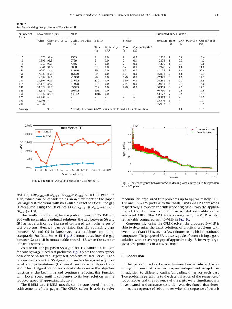
Table 7Results of solving test problems of Data Series III.

Number of

Parts

Lower bound (LB) MILP Simulated annealing (SA)

Value Closeness (LB-OS)

(%)

Optimal solution

(OS)

E-MILP B-MILP Solution Time

(s)

GAP (SA & OS)

(%)

GAP (SA & LB)

(%)Time

(s)

Optimality

GAP

Time

(s)

Optimality GAP

(%)

5 1379 91.4 1509 2 0.0 2 0.0 1509 1 0.0 9.4

10 2695 96.3 2799 2 0.0 2 0.1 2808 1 0.3 4.2

15 4265 98.1 4346 2 0.0 2 0.0 4376 1 0.7 2.6

20 5341 91.0 5868 57 0.0 57 0.0 5926 2 1.0 11.0

40 9267 84.1 11,019 59 0.0 62 0.0 11,178 3 1.4 20.6

60 14,828 89.8 16,509 69 0.0 85 0.0 16,801 3 1.8 13.3

80 19,582 89.1 21,970 99 0.0 126 0.0 22,379 3 1.9 14.3

100 24,894 90.1 27,632 179 0.0 330 0.0 28,251 5 2.2 13.5

115 28,173 88.2 31,928 218 0.0 734 0.0 32,681 6 2.4 16.0

130 31,022 87.7 35,385 519 0.0 896 0.0 36,358 6 2.7 17.2

145 35,531 89.2 39,812 605 0.0 – – 40,789 6 2.5 14.8

160 38,322 88.9 43,112 1016 0.0 – – 44,177 7 2.5 15.3

175 42,802 – – – – – – 48,572 8 – 13.5

190 46,768 – – – – – – 53,346 9 – 14.1

200 48,042 – – – – – – 55,957 9 – 16.5

Average 90.3 No output because GAMS was unable to find a feasible solution 1.6 13.1

0.0%

5.0%

10.0%

15.0%

20.0%

25.0%

5 10 15 20 40 60 80 100 115 130 145 160 175 190 200

GA

P (%

)

Number of Parts

Data Series IIISA&LB

SA&OS

Fig. 8. The gap of SA&OS and SA&LB for Data Series III.Fig. 9. The convergence behavior of SA in dealing with a large-sized test problem

with 200 parts.

M.H. Fazel Zarandi et al. / Computers & Operations Research 40 (2013) 1420–1434 1431

and OS, GAPSA&OS¼((SAvalue�OSvalue)/OSvalue)�100, is equal to1.3%, which can be considered as an achievement of the paper.For large test problems with no available exact solutions, the gapis computed using the LB values as GAPSA&LB¼((SAvalue�LBvalue)/LBvalue)�100.

The results indicate that, for the problem sizes of 175, 190 and200 with no available optimal solutions, the gap between SA andLB has not significantly increased compared with other sizes oftest problems. Hence, it can be stated that the optimality gapsbetween SA and OS in large-sized test problems are ratheracceptable. For Data Series III, Fig. 8 demonstrates how the gapbetween SA and LB becomes stable around 15% when the numberof parts increases.

As a result, the proposed SA algorithm is qualified to be usedfor solving large-sized test problems. Fig. 9 plots the convergencebehavior of SA for the largest test problem of Data Series II anddemonstrates how the SA algorithm searches for a good sequenceamid 200! permutations (the worst case for a problem of size200). The SA algorithm causes a drastic decrease in the objectivefunction at the beginning and continues reducing this functionwith lower speed until it converges to its best solution with areduced speed of approximately zero.

The E-MILP and B-MILP models can be considered the otherachievements of the paper. The CPLEX solver is able to solve

medium- or large-sized test problems up to approximately 115–130 and 160–175 parts with the B-MILP and E-MILP approaches,respectively. However, the difference originates from the applica-tion of the dominance condition as a valid inequality in theenhanced MILP. The CPU time savings using E-MILP is alsoremarkable compared with B-MILP in Fig. 10.

Consequently, using the CPLEX solver, the proposed E-MILP isable to determine the exact solutions of practical problems witheven more than 175 parts in a few minutes using higher equippedcomputers. The proposed SA is also capable of determining a goodsolution with an average gap of approximately 1% for very large-sized test problems in a few seconds.

6. Conclusion

This paper introduced a new two-machine robotic cell sche-duling problem that considers sequence-dependent setup timesin addition to different loading/unloading times for each part.Two problems pertaining to the determination of the sequence ofrobot moves and the sequence of the parts were simultaneouslyinvestigated. A dominance condition was developed that deter-mines the sequence of robot moves when the sequence of parts is

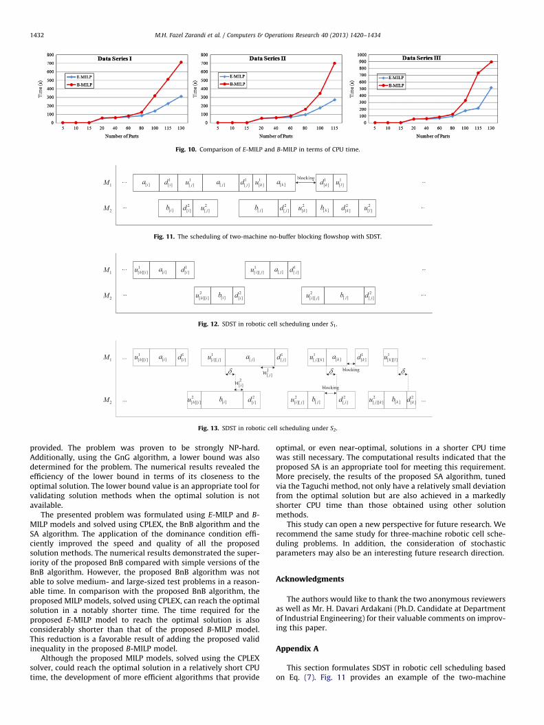
Fig. 10. Comparison of E-MILP and B-MILP in terms of CPU time.

[ ]ia

[ ]ib

1[ ]id

2[ ]id

1[ ]ju

1[ ]ku[ ]ja

[ ]jb

1[ ]jd

2[ ]jd

1M

2M2[ ]ju

2[ ]ku

1[ ]lu[ ]ka 1

[ ]kd

[ ]kb 2[ ]kd

2[ ]lu

Fig. 11. The scheduling of two-machine no-buffer blocking flowshop with SDST.

1[ ][ ]h iu

2[ ][ ]h iu

[ ]ia

[ ]ib

1[ ]id

2[ ]id

1[ ][ ]i ju

2[ ][ ]i ju

[ ]ja

[ ]jb

1[ ]jd

2[ ]jd

1M

2M

Fig. 12. SDST in robotic cell scheduling under S1.

Fig. 13. SDST in robotic cell scheduling under S2.

M.H. Fazel Zarandi et al. / Computers & Operations Research 40 (2013) 1420–14341432

provided. The problem was proven to be strongly NP-hard.Additionally, using the GnG algorithm, a lower bound was alsodetermined for the problem. The numerical results revealed theefficiency of the lower bound in terms of its closeness to theoptimal solution. The lower bound value is an appropriate tool forvalidating solution methods when the optimal solution is notavailable.

The presented problem was formulated using E-MILP and B-MILP models and solved using CPLEX, the BnB algorithm and theSA algorithm. The application of the dominance condition effi-ciently improved the speed and quality of all the proposedsolution methods. The numerical results demonstrated the super-iority of the proposed BnB compared with simple versions of theBnB algorithm. However, the proposed BnB algorithm was notable to solve medium- and large-sized test problems in a reason-able time. In comparison with the proposed BnB algorithm, theproposed MILP models, solved using CPLEX, can reach the optimalsolution in a notably shorter time. The time required for theproposed E-MILP model to reach the optimal solution is alsoconsiderably shorter than that of the proposed B-MILP model.This reduction is a favorable result of adding the proposed validinequality in the proposed B-MILP model.

Although the proposed MILP models, solved using the CPLEXsolver, could reach the optimal solution in a relatively short CPUtime, the development of more efficient algorithms that provide

optimal, or even near-optimal, solutions in a shorter CPU timewas still necessary. The computational results indicated that theproposed SA is an appropriate tool for meeting this requirement.More precisely, the results of the proposed SA algorithm, tunedvia the Taguchi method, not only have a relatively small deviationfrom the optimal solution but are also achieved in a markedlyshorter CPU time than those obtained using other solutionmethods.

This study can open a new perspective for future research. Werecommend the same study for three-machine robotic cell sche-duling problems. In addition, the consideration of stochasticparameters may also be an interesting future research direction.

Acknowledgments

The authors would like to thank the two anonymous reviewersas well as Mr. H. Davari Ardakani (Ph.D. Candidate at Departmentof Industrial Engineering) for their valuable comments on improv-ing this paper.

Appendix A

This section formulates SDST in robotic cell scheduling basedon Eq. (7). Fig. 11 provides an example of the two-machine

M.H. Fazel Zarandi et al. / Computers & Operations Research 40 (2013) 1420–1434 1433

no-buffer blocking flowshop scheduling problem with SDST. Here,instead of the permutation function s, the classical symbol [.] isused to represent the position of the ith, jth and kth jobs in thesequence. Parameters aj and bj are the processing times of the jthjob on M1 and M2, respectively.

Unlike Fig. 11, in 2RCSDST, the setdown and setup operationsmust be executed immediately after and before each job, knownas non-anticipatory [39] (non-separable) setups. The relevance ofSDST in robotic cell scheduling is illustrated in Figs. 12 and 13based on robot move sequences S1 and S2.

In Figs. 12 and 13, ukij denotes the setup operation time of job j

preceded by job i on machine k. The formulation of the SDST inrobotic cell scheduling under S1 and S2 is represented by

s1ij ¼ d2

i þu1ij ¼ ðe

22i þdþe

3i þ3dÞþðe0

j þdþe11ij Þ

s2ij ¼ d1

j þu2ij ¼ ðe

12j þdÞþðe

21ij Þ ð45Þ

s1hij ¼ d1

i þu2hiþu1

ij ¼ ðe12i þdÞþðe

21hi Þþð2dþe

0j þdþe

11ij Þ

s2ij ¼ d2

i þw1j þd1

j þu2ij ¼ ðe

22i þdþe

3i þ2dÞþðw1

j Þþðe12j þdÞþðe

21ij Þ

ð46Þ

In Eq. (46), the SDST of the jth job on M1 (s1hij) is formed from

its two previous jobs parameters.

References

[1] Dawande M, Geismar HN, Sethi SP, Sriskandarajah C. Sequencing andscheduling in robotic cells: recent developments. Journal of Scheduling2005;8:387–426.

[2] Hall NG, Kamoun H, Sriskandarajah C. Scheduling in robotic cells: complexityand steady state analysis. European Journal of Operational Research1998;109:43–65.

[3] Aneja YP, Kamoun H. Scheduling of parts and robot activities in a twomachine robotic cell. Computers & Operations Research 1999;26:297–312.

[4] Bagchi TP, Gupta JND, Sriskandarajah C. A review of TSP based approaches forflowshop scheduling. European Journal of Operational Research 2006;169:816–54.

[5] Crama Y, Kats V, van de Klundert J, Levner E. Cyclic scheduling in roboticflowshops. Annals of Operations Research 2000;96:97–124.

[6] Brauner N. Identical part production in cyclic robotic cells: concepts, over-view and open questions. Discrete Applied Mathematics 2008;156:2480–92.

[7] Sethi SP, Sriskandarajah C, Sorger G, Blazewicz J, Kubiak W. Sequencing ofparts and robot moves in a robotic cell. International Journal of FlexibleManufacturing Systems 1992;4:331–58.

[8] Logendran R, Sriskandarajah C. Sequencing of robot activities and parts intwo-machine robotic cells. International Journal of Production Research1996;34:3447–63.

[9] Hall NG, Kamoun H, Sriskandarajah C. Scheduling in robotic cells: classifica-tion, two and three machine cells. Operations Research 1997;45:421–39.

[10] Crama Y, van de Klundert J. Cyclic scheduling of identical parts in a roboticcell. Operations Research 1997;45:952–65.

[11] Chen H, Chu C, Proth J-M. Sequencing of parts in robotic cells. InternationalJournal of Flexible Manufacturing Systems 1997;9:81–104.

[12] Sriskandarajah C, Hall NG, Kamoun H. Scheduling large robotic cells withoutbuffers. Annals of Operations Research 1998;76:287–321.

[13] Agnetis A. Scheduling no-wait robotic cells with two and three machines.European Journal of Operational Research 2000;123:303–14.

[14] Brauner N, Finke G. Cycles and permutations in robotic cells. Mathematicaland Computer Modelling 2001;34:565–91.

[15] Brauner N, Finke G, Kubiak W. Complexity of one-cycle robotic flow-shops.Journal of Scheduling 2003;6:355–72.

[16] Geismar HN, Dawande M, Sriskandarajah C. Robotic cells with parallelmachines: throughput maximization in constant travel-time cells. Journalof Scheduling 2004;7:375–95.

[17] Neil Geismar H, Dawande M, Sriskandarajah C. Approximation algorithms fork-unit cyclic solutions in robotic cells. European Journal of OperationalResearch 2005;162:291–309.

[18] Akturk MS, Gultekin H, Karasan OE. Robotic cell scheduling with operationalflexibility. Discrete Applied Mathematics 2005;145:334–48.

[19] Gultekin H, Akturk MS, Karasan OE. Cyclic scheduling of a 2-machine roboticcell with tooling constraints. European Journal of Operational Research2006;174:777–96.

[20] Drobouchevitch IG, Sethi SP, Sriskandarajah C. Scheduling dual gripperrobotic cell: one-unit cycles. European Journal of Operational Research2006;171:598–631.

[21] Gultekin H, Akturk MS, Ekin Karasan O. Scheduling in a three-machinerobotic flexible manufacturing cell. Computers & Operations Research2007;34:2463–77.

[22] Gultekin H, Akturk MS, Karasan OE. Scheduling in robotic cells: processflexibility and cell layout. International Journal of Production Research2008;46:2105–21.

[23] Dawande M, Pinedo M, Sriskandarajah C. Multiple part-type production inrobotic cells: equivalence of two real-world models. Manufacturing & ServiceOperations Management 2009;11:210–28.

[24] Drobouchevitch IG, Neil Geismar H, Sriskandarajah C. Throughput optimiza-tion in robotic cells with input and output machine buffers: a comparativestudy of two key models. European Journal of Operational Research2010;206:623–33.

[25] Kats V, Levner E. A faster algorithm for 2-cyclic robotic scheduling with afixed robot route and interval processing times. European Journal of Opera-tional Research 2011;209:51–6.

[26] Yildiz S, Akturk MS, Karasan OE. Bicriteria robotic cell scheduling withcontrollable processing times. International Journal of Production Research2010;49:569–83.

[27] Kimiagari AM, Mosadegh H. Two-machine robotic cell considering differentloading and unloading times. Journal of Industrial Engineering International2011;7:41–52.

[28] Che A, Hu H, Chabrol M, Gourgand M. A polynomial algorithm for multi-robot2-cyclic scheduling in a no-wait robotic cell. Computers & OperationsResearch 2011;38:1275–85.

[29] Zahrouni W, Kamoun H. Transforming part-sequencing problems in arobotic cell into a GTSP. Journal of the Operational Research Society2011;62:114–23.

[30] Yildiz S, Karasan OE, Akturk MS. An analysis of cyclic scheduling problems inrobot centered cells. Computers & Operations Research 2012;39:1290–9.

[31] Suarez R, Rosell J. Feeding sequence selection in a manufacturing cell withfour parallel machines. Robotics and Computer-Integrated Manufacturing2005;21:185–95.

[32] Soukhal A, Martineau P. Resolution of a scheduling problem in a flowshoprobotic cell. European Journal of Operational Research 2005;161:62–72.

[33] Alcaide D, Chu C, Kats V, Levner E, Sierksma G. Cyclic multiple-robotscheduling with time-window constraints using a critical path approach.European Journal of Operational Research 2007;177:147–62.

[34] Brucker P, Kampmeyer T. A general model for cyclic machine schedulingproblems. Discrete Applied Mathematics 2008;156:2561–72.

[35] Yoosefelahi A, Aminnayeri M, Mosadegh H, Davari Ardakani H. Type II roboticassembly line balancing problem: an evolution strategies algorithm for amulti-objective model. Journal of Manufacturing Systems 2012;31:139–51.

[36] Levner E, Kats V, Alcaide Lopez de Pablo D, Cheng TCE. Complexity of cyclicscheduling problems: a state-of-the-art survey. Computers & IndustrialEngineering 2010;59:352–61.

[37] Deineko VG, Steiner G, Xue Z. Robotic-cell scheduling: special polynomiallysolvable cases of the traveling salesman problem on permuted mongematrices. Journal of Combinatorial Optimization 2005;9:381–99.

[38] Laporte G, Asef-Vaziri A, Sriskandarajah C. Some applications of the general-ized travelling salesman problem. Journal of the Operational ResearchSociety 1996;47:1461–7.

[39] Allahverdi A, Ng CT, Cheng TCE, Kovalyov MY. A survey of schedulingproblems with setup times or costs. European Journal of OperationalResearch 2008;187:985–1032.

[40] Gupta JND, Darrow WP. The two-machine sequence dependent flowshopscheduling problem. European Journal of Operational Research1986;24:439–46.

[41] Logendran R, Salmasi N, Sriskandarajah C. Two-machine group schedulingproblems in discrete parts manufacturing with sequence-dependent setups.Computers & Operations Research 2006;33:158–80.

[42] Liao C-J, Juan H-C. An ant colony optimization for single-machine tardinessscheduling with sequence-dependent setups. Computers & OperationsResearch 2007;34:1899–909.

[43] Salmasi N, Logendran R. A heuristic approach for multi-stage sequence-dependent group scheduling problems. Journal of Industrial EngineeringInternational 2008;4:48–58.

[44] Monkman GJ, Hesse S, Steinmann RHS. Robot grippers. Berlin: Wiley; 2007.[45] Huang Y-J, Lee F-F. An automatic machine vision-guided grasping system for

phalaenopsis tissue culture plantlets. Computers and Electronics in Agricul-ture 2010;70:42–51.

[46] Borangiu T, Anton F, Tunaru S, Dogar A, Lvanescu N. Interactive learning ofscene-robot models based on al techniques. In: Alexandre D, Gerard M, CarlosEPereira, editors. Information control problems in manufacturing 2006.Oxford: Elsevier Science Ltd.; 2006. p. 203–8.

[47] Allahverdi A, Aldowaisan T. Minimizing total completion time in a no-waitflowshop with sequence-dependent additive changeover times. Journal of theOperational Research Society 2001;52:449–62.

[48] Toth P. Optimization engineering techniques for the exact solution of NP-hard combinatorial optimization problems. European Journal of OperationalResearch 2000;125:222–38.

[49] Zhang R, Wu C. A hybrid immune simulated annealing algorithm for the jobshop scheduling problem. Applied Soft Computing 2010;10:79–89.

[50] Geng X, Chen Z, Yang W, Shi D, Zhao K. Solving the traveling salesmanproblem based on an adaptive simulated annealing algorithm with greedysearch. Applied Soft Computing 2011;11:3680–9.

M.H. Fazel Zarandi et al. / Computers & Operations Research 40 (2013) 1420–14341434

[51] Mosadegh H, Zandieh M, Fatemi Ghomi SMT. Simultaneous solving ofbalancing and sequencing problems with station-dependent assembly timesfor mixed-model assembly lines. Applied Soft Computing 2012;12:1359–70.

[52] Lv P, Yuan L, Zhang J. Cloud theory-based simulated annealing algorithm andapplication. Engineering Applications of Artificial Intelligence 2009;22:742–9.

[53] Kirkpatrick S. Optimization by simulated annealing: quantitative studies.Journal of Statistical Physics 1984;34:975–86.

[54] Taguchi G. Introduction to quality engineering: designing quality intoproducts and processes. White Plains: Asian Productivity Organization; 1986.

[55] Naderi B, Zandieh M, Fatemi Ghomi SMT. Scheduling job shop problems withsequence-dependent setup times. International Journal of Production Research2009;47:5959–76.

[56] Mosadegh H, Fatemi Ghomi SMT, Zandieh M. Simultaneous solving ofbalancing and sequencing problems in mixed-model assembly line systems.International Journal of Production Research 2012:1–23 iFirst.