Two meta-heuristics for three-stage assembly flowshop scheduling with sequence-dependent setup times

ORIGINAL ARTICLE

Two meta-heuristics for three-stage assembly flowshopscheduling with sequence-dependent setup times

Sara Hatami & Sadalah Ebrahimnejad &

Reza Tavakkoli-Moghaddam & Yasaman Maboudian

Received: 16 November 2009 /Accepted: 10 February 2010 /Published online: 9 April 2010# Springer-Verlag London Limited 2010

Abstract In this paper, we consider a three-stage assemblyflowshop scheduling problem with bi-objectives, namelythe mean flow time and maximum tardiness. This problemcan be considered as a production system model consistingof three stages: (1) different production operations are donein parallel, concurrently and independently, (2) the manu-factured parts are collected and transferred to the next stage,and (3) these parts are assembled into final products. In thispaper, sequence-dependent setup times and transfer timesare also considered as two important presumptions in orderto make the problem more realistic. We present a novelmathematical model for a production system with a newlower bound for the given problem. Obtaining an optimalsolution for this type of complex, large-sized problem inreasonable computational time by using traditionalapproaches and optimization tools is extremely difficult.Thus, we propose two meta-heuristics, namely simulated

annealing and tabu search, to solve a number of testproblems generated at random. Finally, the computationalresults are illustrated and compared in order to show theefficiency of the foregoing meta-heuristics.

Keywords Assembly flowshop scheduling .Mean flowtime .Maximum tardiness . Sequence-dependent setuptimes . Simulated annealing . Tabu search

1 Introduction

Global competition and the ability to respond to the changingdemand markets, while keeping the costs down, are some ofthe key elements in designing effective production systems.Assembly flowshop is a combinatorial production system, inwhich different sets of parts are manufactured independentlyon parallel production lines (or machines), and then they areassembled into final products. These production-assemblysystems can be used as a way to produce a variety of goodsby assembling and combining different sets of parts andsubassemblies. From the scheduling perspective, thesesystems are modeled as a two-stage assembly flowshopscheduling problem (AFSP) [1]. In this problem, jobs (orproducts) are performed in two stages. At the first stage,parts of each job are manufactured concurrently on parallelmachines, and at the second stage, they are assembled tomake the final product. This model does not consider therequired operation for collecting and transporting themanufactured parts from production site to assembly site.To have a more realistic model, another stage can beconsidered as a middle stage between the production andassembly stages, called transportation stage, in which partsand subassemblies are collected and transferred fromproduction stage to assembly stage. This stage is important

S. HatamiDepartment of Industrial Engineering,Islamic Azad University-Ghazvin Branch,Ghazvin, Iran

S. Ebrahimnejad (*)Department of Industrial Engineering,Islamic Azad University-Karaj Branch,Karaj, Irane-mail: [email protected]

R. Tavakkoli-MoghaddamDepartment of Industrial Engineering and Center of Excellencefor Intelligence Based Experimental Mechanics,College of Engineering, University of Tehran,Tehran, Iran

Y. MaboudianDepartment of Industrial Engineering,Khaje Nasir University of Technology,Tehran, Iran

Int J Adv Manuf Technol (2010) 50:1153–1164DOI 10.1007/s00170-010-2579-5

especially when parts are manufactured in multiple produc-tion sites. Therefore, a three-stage assembly flowshopscheduling problem is a generalization of a two-stage AFSP.

In a three-stage assembly flowshop scheduling problem,there are n jobs to be scheduled. Each job consists of mparts. There are m parallel and independent machines at thefirst stage, and each machine is assigned to process aspecific part. Once the operations associated with all partsof a job are performed at the first stage, parts are collectedand transferred to the assembly machine through the secondstage (transportation stage); then a single machine at thethird stage assembles all m parts together to complete a job.

The model considered in this paper is an extension ofmodel proposed by Koulamas and Kyparisis [1]. Theyintroduced three-stage assembly flowshop, in which themiddle stage is dedicated to components collection andtransformation. However in our paper, we add sequence-dependent setup times (SDST) to their model in order tomake the model real. The applications for two-stageassembly flowshop scheduling problems are mentioned inthe literature. Potts et al. [2] considered an application inpersonal computer manufacturing where central processingunits, hard disks, monitors, keyboards, and the like aremanufactured separately at the first stage. Then bycustomer specification, all the required components areassembled to a packaging station at the second stage. Lee etal. [3] considered an application in a fire engine assemblyplant, in which the body and chassis of fire engines areproduced in parallel and in two different departments. Aftercompletion of body and chassis and delivery of the engine(purchased from outside), they are fed to the assembly linein order to assemble the final fire engine. Our presentedmodel can be applicable to an electronic industry, liketelevision making company or air conditioner. It is clearthat two-stage assembly flowshop scheduling problems arenot the realistic models because the consumed time, whichis spent to collect and transfer components from first stageto second stage, is not considered. Especially, when we tryto simulate the two-stage assembly problem, in which itsproduction systems have multi-plant facilities and a finalassembly plant. In these cases, components collection andtransformation times are really important to be considered,and it is also necessary even when all operations (includingthe assembly) are performed in the same production facility.In the most of these facilities, machines at the first stage ofthe production line are located throughout the factory floorand the assembly machine is located near the output area ofthe production facility. Machines at the first stage areflexible to change based on their producing program inorder to produce another specific components with differentcharacteristics (e.g., different kinds of keyboards orprocessing units for each customer specification). It needssetup time consideration to adopt machines.

In the scheduling literature, Koulamas and Kyparisis [1]considered a three-stage assembly flowshop schedulingproblem with the objective of minimizing the makespanand analyzed the worst-case ratio bound for several heuris-tics. Lee et al. [3] studied a two-stage AFSP with consideringtwo machines at the first stage. Tozkapan et al. [4] considereda two-stage AFSP by minimizing the total weighted flowtime. They developed a procedure of a lower bound,dominance criterion, and incorporated them into a branch-and-bound procedure. They also used a heuristic procedure toderive an initial upper bound. Al-Anzi and Allahverdi [5]addressed the model presented by Tozkapan et al. [4] andtried to minimize the total completion time of all jobs. Theyproposed a simulated annealing (SA), a tabu search (TS), anda hybrid tabu search heuristic for general cases.

Allahverdi and Al-Anzi [6] considered distributeddatabase systems and computer manufacturing as anassembly flowshop scheduling problem by minimizing themaximum lateness. They formulated the problem, obtaineda dominance relation, and proposed three heuristics: particleswarm optimization (PSO), tabu search (TS), and earlinessdue date (EDD). Al-Anzi and Allahverdi [7] addressed atwo-stage AFSP by considering sequence-independentsetup times that minimizes the maximum lateness. Theyproposed a self-adaptive differential evolution (SDE) andcompared it with PSO, TS, and EDD. Allahverdi and Al-Anzi [8] addressed a two-stage AFSP with the weightedsum of the makespan and mean completion times. Theyproposed three heuristics to solve the given problem: antcolony optimization and self-adaptive differential evolution(SDE). Tavakkoli-Moghaddam et al. [9] presented aflexible flow line scheduling problem with processorblocking and without intermediate buffers. The flexibleflow line consists of several processing stages in series, withor without intermediate buffers, with each stage having oneor more identical parallel processors. They proposed a newnested variable neighborhood search embedded to a mem-etic algorithm in order to solve this problem. Gharehgozli etal. [10] presented a new mixed-integer goal programmingmodel for a parallel machine scheduling problem withsequence-dependent setup times and release dates. Theyconsidered the hypothesis of fuzzy processing time'sknowledge and two fuzzy objectives, namely the totalweighted flow time and the total weighted tardiness. Al-Anzi and Allahverdi [11] considered a two-stage AFSPwith the objective of minimizing a weighted sum ofmakespan and maximum lateness and proposed threeheuristics, TS, PSO, and SDE to solve the NP-hard model.

In this paper, we consider a three-stage AFSP withsequence-dependent setup times at the first stage, whereeach machine requires a setup time before starting theoperation. In this problem, the mean flow time andmaximum tardiness are considered as two criteria. To our

1154 Int J Adv Manuf Technol (2010) 50:1153–1164

knowledge, this is the first effort that considers the problemwith sequence-dependent setup times and two foregoingcriteria. The remainder of this paper is organized asfollows: Section 2 presents a complete definition alongwith presumptions, constraints, and a new nonlinear modelof the considered problem and develops a lower bound forthe makespan in order to generate random due dates forcomputational experiments. In Section 3, two heuristics areproposed, namely SA and TS, in order to solve theconsidered model. In Section 4, the performance of twoproposed initial solutions are compared as heuristics’ startpoint. Computational experiments and the numerical com-parisons of the proposed heuristics are provided inSection 5. Finally, Section 6 consists of conclusions andsome possible areas for the future research.

2 Problem definition

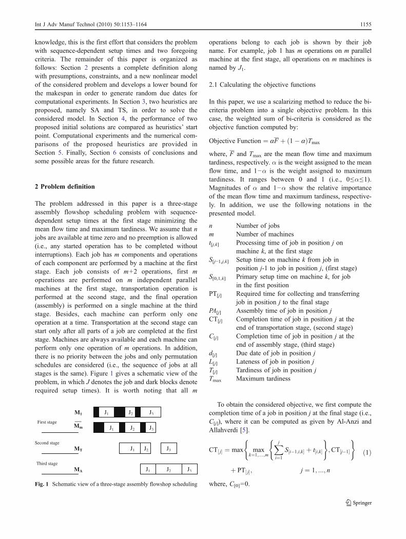
The problem addressed in this paper is a three-stageassembly flowshop scheduling problem with sequence-dependent setup times at the first stage minimizing themean flow time and maximum tardiness. We assume that njobs are available at time zero and no preemption is allowed(i.e., any started operation has to be completed withoutinterruptions). Each job has m components and operationsof each component are performed by a machine at the firststage. Each job consists of m+2 operations, first moperations are performed on m independent parallelmachines at the first stage, transportation operation isperformed at the second stage, and the final operation(assembly) is performed on a single machine at the thirdstage. Besides, each machine can perform only oneoperation at a time. Transportation at the second stage canstart only after all parts of a job are completed at the firststage. Machines are always available and each machine canperform only one operation of m operations. In addition,there is no priority between the jobs and only permutationschedules are considered (i.e., the sequence of jobs at allstages is the same). Figure 1 gives a schematic view of theproblem, in which J denotes the job and dark blocks denoterequired setup times). It is worth noting that all m

operations belong to each job is shown by their jobname. For example, job 1 has m operations on m parallelmachine at the first stage, all operations on m machines isnamed by J1.

2.1 Calculating the objective functions

In this paper, we use a scalarizing method to reduce the bi-criteria problem into a single objective problem. In thiscase, the weighted sum of bi-criteria is considered as theobjective function computed by:

Objective Function ¼ aF þ 1� að ÞTmax

where, F and Tmax are the mean flow time and maximumtardiness, respectively. α is the weight assigned to the meanflow time, and 1−α is the weight assigned to maximumtardiness. It ranges between 0 and 1 (i.e., 0≤α≤1).Magnitudes of α and 1−α show the relative importanceof the mean flow time and maximum tardiness, respective-ly. In addition, we use the following notations in thepresented model.

n Number of jobsm Number of machinest[j,k] Processing time of job in position j on

machine k, at the first stageS[j−1,j,k] Setup time on machine k from job in

position j-1 to job in position j, (first stage)S[0,1,k] Primary setup time on machine k, for job

in the first positionPT[j] Required time for collecting and transferring

job in position j to the final stagePA[j] Assembly time of job in position jCT[j] Completion time of job in position j at the

end of transportation stage, (second stage)C[j] Completion time of job in position j at the

end of assembly stage, (third stage)d[j] Due date of job in position jL[j] Lateness of job in position jT[j] Tardiness of job in position jTmax Maximum tardiness

To obtain the considered objective, we first compute thecompletion time of a job in position j at the final stage (i.e.,C[j]), where it can be computed as given by Al-Anzi andAllahverdi [5].

CT j½ � ¼ max maxk¼1;::::;m

Xji¼1

S i�1;i;k½ � þ t i;k½ �

( );CT j�1½ �

( )

þ PT j½ �; j ¼ 1; :::; n

ð1Þ

where, C[0]=0.

J3

J1

J1

J1

J2

J2

J2

J3

J3

J3 J1 J2

M1

Mm

MT

MA

First stage

Second stage

Third stage

Fig. 1 Schematic view of a three-stage assembly flowshop scheduling

Int J Adv Manuf Technol (2010) 50:1153–1164 1155

Equation 1 shows the completion time of job in positionj, at the end of the transportation stage. The completiontime of job in position j at the final stage can be computedaccording to Eq. 2.

C j½ � ¼ max CT j½ �;C j�1½ �� þ PA j½ � ; j ¼ 1; ::::; n ð2Þ

F is computed by:

F ¼

Pnj¼1

C j½ �

nð3Þ

It is assumed that all jobs are ready at time zero, (r[j]=0; theready time of job in position j at the system). Therefore, theflow time of job in position j is equal to C[j]−r[j], or simply C[j].

To compute the second criterion, Tmax, first we shouldcompute the lateness by Eq. 4, then maximum tardiness canbe computed according to Eqs. 5 and 6.

L j½ � ¼ C j½ � � d j½ � ; j ¼ 1; :::; n ð4Þ

T j½ � ¼ max 0; L j½ ��

; j ¼ 1; :::; n ð5Þ

Tmax ¼ maxn

j¼1T½j�� ð6Þ

2.2 Mathematical model

This section presents a non-linear model for the givenproblem with the following notations:

1. Parameters:k Machine at the first stage.Sq,j,k Setup time on machine k from job q to job j (at the

first stage).S0,j,k Primary setup time on machine k if job j is in the

first position (first stage).tj,k Operation time of job j on machine k, at the first

stage.PTj Required time for collecting and transporting job j

(at the second stage).PAj Operation time of job j on assembly machine.

2. Variables:x[i] j = 1, if job j is in position i of the sequence;

otherwise, it is 0.y[i] Completion time of all m operations of the job

in position i at the first stage.A[i],j,k Sum of operation times on machine k from job

in the first position to job in position i, wherejob j is in position i.

Z[i] Start time of transportation operation of job inposition i.

w[i] Start time of assembly operation of job in position i.

min : Z ¼ aXni¼1

C i½ �n

!þ 1� að Þ Tmaxð Þ ð7Þ

s.t.

Xni¼1

x i½ � j ¼ 1 ; 8j ð8Þ

Xnj¼1

x i½ � j ¼ 1 ; 8i ð9Þ

A 1½ �;j;k ¼ x1j � tj;k þ S0;j;k� �

; 8j; k ð10Þ

A i½ �;j;k ¼ x i½ �j � tj;k þXn

q¼1;q 6¼j

x i�1½ �q � Sq;j;k� � !

þXn

l¼1;l 6¼j

A i�1½ �;l;k ; 8j; k; i ¼ 2; 3; :::n

ð11Þ

A i½ �;j;k � y i½ � ; 8i ð12Þ

y i½ � � Z i½ � ; 8i ð13Þ

CT i½ � ¼ Z i½ � þXnj¼1

x i½ �j � PTj

� �; 8i ð14Þ

CT i�1½ � � Z i½ � ; 8i ð15Þ

CT i½ � � w i½ � ; 8i ð16Þ

C i½ � ¼ w i½ � þXnj¼1

x i½ �j � PAj

� �; 8i ð17Þ

C i�1½ � � w i½ � ; 8i ð18Þ


T i½ � � C i½ � �Xnj¼1

x i½ �j � d i½ ��

; 8i ð19Þ

T i½ � � 0 ; 8i ð20Þ

T i½ � � Tmax ; 8i ð21Þ

xij 2 0; 1f g ; 8i; j ð22Þ

Si;i;k ¼ 0 ; 8i; k ð23Þ

C 0½ � ¼ CT 0½ � ¼ 0 ð24ÞEquation 7 presents the objective function. Equations 8

and 9 show that each job can only be placed in one positionand only one job can be placed in each position, respective-ly. Equations 10 and 11 calculate A[1],j,k and A[i],j,k,respectively. Equation 12 shows the time when all moperations of job in position i are completed. Equation 13shows the necessity of all m operations of job in position ibeing completed in stage one, before starting its transporta-tion operation. Equation 14 calculates the completion time ofjob in position i in stage two. Equation 15 shows thenecessity of transportation of job in position i−1 beingcompleted before starting the transportation of job in positioni. Equation 16 shows that the transportation of job in positioni must be completed at stage two, before starting of itsassembly operation at the final stage. Equation 17 calculatesthe completion time of job in position i at assembly stage.Equation 18 shows that the assembly operation of job inposition i cannot be started if the assembly machine is busyfor assembling a job in position i-1. Equations 19 and 20calculate the tardiness of job in position i. Constraint 21calculates the maximum tardiness of jobs. Furthermore,Eq. 22 indicates that xij can only take zero/one value.

2.3 Proposed LB bound

To produce an example and calculate the second objectivefunction (i.e., maximum tardiness), due dates should begenerated based on the method introduced by Loukilet al. [12]. Due dates are uniformly distributed in theinterval p 1�ð½ T � R

2Þ; p 1� T þ R2

� ��, where p denotes thetime which all the jobs are completed (usually p isconsidered as a lower bound (LB)) [7]. T is the tardinessfactor and R denotes the relative range of due dates. Rabadiet al. [13] defined a matrix [AP] as shown in Eq. 25 thatcombines the processing times and setup times in onematrix.

APqjk ¼ Sqjk þ tjk ; 8j; k; q ¼ 0; 1; :::; n ð25Þwhere, APqjk is the adjusted processing time from job q tojob j on machine k (first stage). Then we have k numbers of[AP](n+1)×n matrix for each parallel machine. Also, forevery j and k, MAPjk is defined as the minimum adjustedprocessing time of job j, on machine k, which is computedby:

MAPjk ¼ minq¼0;1;:::n

APqjk� �

: q 6¼ j; 8j; k ð26Þ

Let:

SUMMAPk ¼Xnj¼1

MAPjk ; 8k ð27Þ

SUMMAPk is the summation of MAPjk on each machine andcan be considered as a lower bound of completion times oneach machine for the first stage.

To begin the second stage, all m operations of each job atthe first stage must be completed. As a result, a lowerbound of the first stage (i.e., LBST1) is calculated by:

LBST1 ¼ maxk¼1;2;::;m

SUMMAPkð Þ ð28Þ

In general, by the use of Eq. 28, a lower bound for theconsidered problem is calculated by:

LB ¼ max LBST1 þminj

PTj þminj

PAj;Xnj¼1

PTj

!þmin

jPAj

( ); 8i ð29Þ

LBST1 denotes the obtained lower bound of the first stage,minj

PTj, denotes the minimum transportation time at the

second stage, and minj

PAj, denotes the minimum assembly

time at the third stage.Pnj¼1

PTj

!þmin

jPAj denotes the

case where the first stage is not considered (i.e., manufac-

tured parts are purchased). In this case,Pnj¼1

PTj denotes the

summation of all transportation times and minj

PAj is theminimum assembly time at the third stage.

To prove the validity of the proposed LB, severalproblems by different numbers of jobs (n; i.e., 20, 30, 40,50, 60, and 70) [7], the first stage parallel machines (m; i.e.,


2, 4, 6, and 8) [11], and weights of objectives (α; i.e., 0.2,0.4, 0.6, and 0.8) [8] are considered. There are differentvalues for T and R factors used in several references [6, 7,11]. Then 0.5 and 0.8 are chosen for T and 0.2, 0.4 and 0.6are chosen for R. Finally, 6� 4� 4� 2� 3 ¼ 576 combi-nations are produced with different values of n, m,α, R, andT.

In the first and third stages, processing times are integersand randomly generated from uniform distribution (1, 100)on all m first stage machines and single third stage machine.In the second stage, processing times are integers as welland generated randomly from uniform distribution (1, 10)on single second stage machine [1]. Setup times areintegers and randomly generated from uniform distribution(1, 20) on all m machines [14]. For each combination, 50problems are produced, in which each problem produces15,000 random sequences. By comparing all sequences,jobs completion times, and proposed LB method value, lessobtained value belongs to the proposed LB method.

3 Two meta-heuristic methods

The considered model is belong to the (AF(m,1,1)//)1 groupand this kind of problem is a general form of (AF(m,1)//)2

and (F3//),3 it is accepted that the model is NP-hard [3].Accordingly, the considered problem is NP-hard in a strongsense. Since this problem is strongly NP-hard, especially byadding SDST consideration, it is strongly suggested tofocus on heuristic or meta-heuristic based approaches tosolve such a hard problem. Furthermore to solve thismodel, two more applicable meta-heuristics are suggested.

To solve the presented model, we propose two heuristicsbased on SA and TS methods explained in Sections 3.1 and3.2, respectively.

3.1 Simulated annealing

SA is named because of its analogy to the process ofphysical annealing in solids, in which a crystalline solid isheated and then allowed to cool very slowly until it

achieves its most regular possible crystal lattice configura-tion. SA is an iterative technique that is not population-based algorithm, such as genetic algorithm. It considersonly one possible solution in each meta-task instead of agroup of possible ones. It is one of the famous meta-heuristics that has been used to solve scheduling problems[15–17]. SA solutions are represented as the order of jobentrance to production line. Each job can be once a time inthe job sequence and all jobs have to be existed. Forexample, 2-3-5-1-4 can be an example for the job sequencefor a production line with five jobs. SA uses an iterativeprocedure that allows poorer solutions to be acceptedprobabilistically and tries to find better solution amongsolution space [18–21]. A system temperature determinesprobability that decreases for each iteration. When thesystem temperature drops (cools), acceptance of poorersolutions gets more difficult. The initial or starting systemtemperatures (T0) is found by accepting an inferiorcandidate solution (Δ) and accept the inferior solution bythe probability of P [21–24]. T0 is obtained by T0 ¼ �Δ

LnðPÞ.The structure of a general SA is as follows. Initial or T0

is set by mentioned procedure. A certain number ofiterations are done at each temperature (Nstep; i.e., innerloop); the first initial possible solution is selected (currentsolution) from possible solution space (the rules of makinginitial solution will be presented in Section 4), new mutatedsolution which is created by a random exchange of thepositions of two jobs in the sequence (on the currentsolution) as the current solution neighborhood N(ω). Forexample, it is shown in Fig. 2, five jobs are considered, andthen positions 2 and 4 are randomly selected for exchangeto make a new possible solution. A comparison is madebetween the objective values of the current solution and thenew generated solution, those are respectively denoted asf (ωn) and f (ωn+1). If the new solution (i.e., mutatedsolution) improves the objective value, it will be consideredas the new current solution to continue the annealing process;otherwise, the new solution is accepted as the new currentsolution with the following probability (y) by generating arandom number R∈[0,1] if y>R; else, the current solution isnot changed, where Ti is the current temperature.

y ¼ ln � f wnþ1ð Þ � f wnð ÞTi

� �

After doing a certain number of iteration (i.e., Nstep) onTi or the current temperature, the system temperature isreduced by the percentage of the current value that isdefined as cooling factor, (dt (<1), Ti ¼ Ti�1 � dt). In theouter loop, Ti value varies from a relatively large value (i.e.,initial temperature, T0) to a small value close to 0 (i.e., finaltemperature, Tf). The proposed SA stops when the finaltemperature reaches to the steady state.

1 Three-stage assembly flowshop problem with m parallel machine atthe first stage and single machine at the second and third stages2 Two-stage assembly flowshop problem with m parallel machine atthe first stage and single machine at the second stage3 Three machine flowshop

1 2 3 4 5 1 4 3 2 5

ω ωN( )

Fig. 2 Generating a neighborhood solution


The algorithmic description of the proposed SA is asfollows.

Initialize parameters T0, Nstep, i, dt, TfInitialized counter n=0, i=0Do (outside loop)Set n=0Generate initial solution ω0: set ωBest=ω0

Do (inside loop)Generate neighboring

Solution N(ω)→ωn+1 by operation (ωn→ωn+1)If f (ωn+1)≤ f (ωn) thenωn=ωn+1 : set n ¼ nþ 1 ElseGenerate random R → u(0,1)

If y ¼ e�f wnþ1ð Þ�f wnð Þ

Ti > R then ωn=ωn+1: set n ¼ nþ 1 Elseωn=ωn: set n ¼ nþ 1

End ifUpdate ωBest

Loop until (n≤Nstep)i← i+1Ti ¼ Ti�1 � dt,Loop until frozen (meet Tf or less than it)

3.2 Tabu search

TS is a meta-heuristic method proposed by Glover [25, 26].It is a local search method that has successful applicationsin solving hard optimization problems [27–29]. TS can bedescribed as a local search technique and enhancement of awell-known hill-climbing heuristic method. Exploitation ofadaptive or flexible forms of memory is a distinguishablecharacteristic of TS in order to penetrate complexities, suchas avoiding being trapped in a local minimum. Theprocedure starts with a feasible initial solution; it can be arandom one or other heuristic output. The initial solution isstored as the current and best solution. Then, entireneighborhood of the current solution is evaluated and themove with the smallest objective value is identified. If it is

not on the tabu list, it is considered as the new currentsolution. A new current solution is generated at each time.Then the implemented move is added to the tabu list. If it isoverloaded, the oldest move is removed from the tabu list.To avoid returning to local optima, a tabu list is used toavoid making the recent moves. Besides, if the new solutionis better than the current best solution, it is stored as a newbest solution. TS proceed iteratively from one solution toanother until a chosen termination criterion is met.

There are various methods to generate initial solutions.In this paper, the initial solution is selected from possiblesolution space by the rules presented in Section 4. Theneighborhood structure is a defined function that transformsa solution to other solutions and it is usually called a move.For example considering a current solution as 1-2-3-4, allfeasible pairwise exchanges can make neighbor solutions asfollows: 2-1-3-4, 1-3-2-4, 1-2-4-3, 4-2-3-1, 3-2-1-4, and 1-4-3-2. In other words, we produce feasible solutions basedon the current solution, those which differs only in two jobpositions compared to the current one. For example, the lastproduced solution (1-4-3-2) is differed in the second andforth positions (two positions) compared to the currentsolution. We can extend our neighborhood structure tomore than a two-position exchange. If the problem has njobs to be scheduled and we are permitted to exchange k

compositions, then we will havenk

� sequences as

neighborhood or candidate solutions.Because the process does not visit the previous steps, the

tabu list is created. The attributes of moves are stored inthe tabu list. In this paper, we memorize in the tabu list, theposition of the jobs that are exchanged with each other inthe neighborhood structure to make new solutions from thecurrent solution. Each attribute of moves can exist in thetabu list for a certain number of iterations, which meanseach tabu list has a length that can accommodate only acertain number of attributes of moves in it. The size of thetabu list must be large enough to prevent meeting thevisited solutions, but small enough not to ban too many

0

10

20

30

40

50

20 30 40 50 60 70

SPT EDD

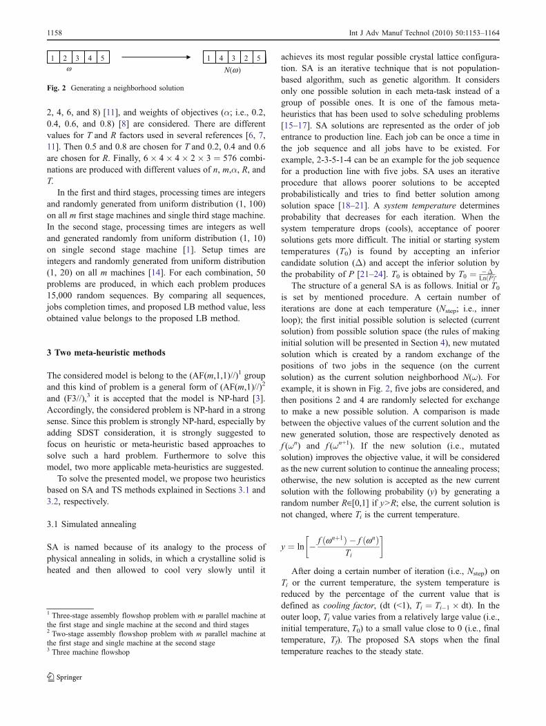
Fig. 3 Average numbers of times best (out 50) versus the number ofjobs (n)

05

101520253035404550

2 4 6 8

SPT EDD

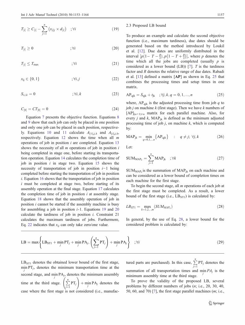
Fig. 4 Average of number of times best (out 50) versus the number ofthe first parallel machines


moves. After implementing the neighbor structure, the bestneighbor is selected and its move attribute is added to theend of the tabu list. The “old” attributes of the tabu list areremoved if it is overloaded. The length of the tabu list isindicated by L. An assumed number of visited solutions (oran assumed number of algorithm iteration) is considered forthe stopping criterion and indicated by Imax. The algorith-mic description of the TS is as follows [27]:

Repeat Imax timesBegin

Randomly swap jobs in the positions of j and kwhere (j,k) is not in the tabu list LLet OFC=value of the objective function afterswap

Reverse swapFor all possible positions of j and k

If (j,k) is not in the tabu list L thenBegin

Swap jobs in positions of j and kLet OFN=value of the objective functionafter the swapIf OFN<OFC, thenSet (j1,k1)=(j,k)OFC=OFNEnd ifReverse swap

End ifEnd for

Swap the jobs in positions of j1 and k1

Add (j1,k1) to front of the tabu list LIF the maximum size of the tabu list is exceeded then

Delete the item at the end of the tabu list LEnd if

End repeatEnd heuristic

4 Proposed initial solution

In general, a random solution is used as the initial solutionin SA and TS algorithms; but in this paper, we try to use aninitial that is not randomly selected. Two famous rules [1,6–8], namely shortest processing time (SPT) and EDD areused to make two suggested initials, which potentially canbe good starting points to search the solution spaceaccording to the considered objectives. These initialsolutions are as follows:

Initial (1):

Step 1: perform the SPT rule independently for eachparallel machine at stage one.

Note: to calculate processing time for each job oneach parallel machine at the first stage, use Eq. 26to obtain mixed processing and setup times.

Step 2: calculate the mean flow time (F) and themaximum tardiness (Tmax) for each obtainedsequence.

Step 3: determine the sequence with the minimumobjective value (aF þ 1� að ÞTmax).

Step 4: consider the obtained sequence as Initial (1).

Initial (2)

Step 1: Consider the due dates of all jobs.Step 2: Sort all jobs by use of the EDD rule.Step 3: Consider the obtained sequence as Initial (2).

We evaluate the average performance of two suggestedinitials by producing different problems that is described inSection 2.3. From every 576 base problems, 50 kinds ofeach one are produced and the number of best times thateach initial obtained the best objective value is counted.The related results are shown in Figs. 3, 4, and 5. Figure 3

05

101520253035404550

0.2 0.4 0.6 0.8

SPT EDD

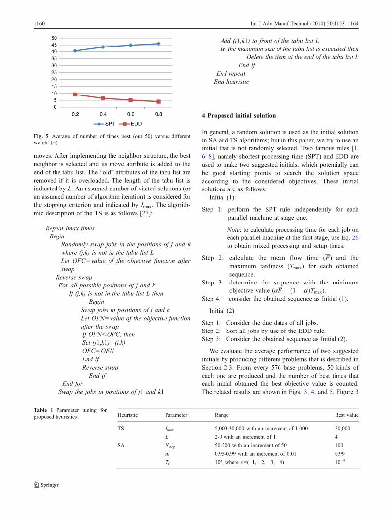
Fig. 5 Average of number of times best (out 50) versus differentweight (α)

Heuristic Parameter Range Best value

TS Imax 5,000-30,000 with an increment of 1,000 20,000

L 2-9 with an increment of 1 4

SA Nstep 50-200 with an increment of 50 100

dt 0.95-0.99 with an increment of 0.01 0.99

Tf 10x, where x=(−1, −2, −3, −4) 10−4

Table 1 Parameter tuning forproposed heuristics


shows the average number of times that the best objectivevalue (aF þ 1� að ÞTmax) are achieved versus the numberof jobs. Figure 4 shows the average of number of times thatthe best objective value is achieved versus the number ofthe first parallel machines. Figure 5 shows the averagenumber of times that the best objective value is achievedversus the number of alphas (α). It can be seen that the firstsuggested initial solution has a bigger number of the besttimes in all figures and then this solution uses as initialsolutions obtained by SA and TS methods instead ofrandom solutions.

5 Computational results

In this section, the method used to set the heuristicsparameters is presented and then the performance of theproposed heuristic in solving the considered problem isevaluated.

n m α R T SA TS

F Tmax F Tmax

20 2 0.2 0.5 0.2 665.1000 196.2000 729.3500 237.9500

20 2 0.4 0.5 0.2 692.3000 214.2000 721.4000 228.5000

20 2 0.6 0.5 0.2 677.1500 195.6500 693.4000 222.1500

20 2 0.8 0.5 0.2 644.5500 203.5500 642.4500 191.1000

30 2 0.2 0.5 0.4 995.7600 278.7000 1056.1000 375.7000

30 2 0.4 0.5 0.4 1,084.1000 376.9000 1,046.6000 360.2000

30 2 0.6 0.5 0.4 938.0333 241.4333 1,043.6000 306.3000

30 2 0.8 0.5 0.4 1,015.8000 343.8000 1,018.3000 310.7000

30 4 0.2 0.8 0.2 1,000.6000 209.5000 1,051.2000 330.2000

30 4 0.4 0.8 0.2 998.0000 267.6333 1,130.0000 364.1000

30 4 0.6 0.8 0.2 1,009.1000 226.8000 1,116.3000 388.7000

30 4 0.8 0.8 0.2 1,019.1000 317.1000 1,066.6000 380.9000

30 6 0.2 0.8 0.6 1,018.2000 597.8000 1,098.7000 680.5000

30 6 0.4 0.8 0.6 985.3000 542.1667 1,031.1000 612.5000

30 6 0.6 0.8 0.6 1,051.4000 605.7000 1,109.8000 676.6000

30 6 0.8 0.8 0.6 1,031.6000 613.4000 1,073.2000 651.4000

Table 2 Objective values(F and Tmax) for our proposedTS and SA

Table 3 Overall average MEP and Std. of two heuristics

n m SA TS

MEP Std. MEP Std.

20 2 0.0019 0.0110 0.0183 0.0455

20 4 0.0018 0.0212 0.0105 0.0267

20 6 0.0025 0.0162 0.0148 0.0396

20 8 0.0034 0.0264 0.0219 0.0298

30 2 0.0021 0.0210 0.0116 0.0352

30 4 0.0029 0.0160 0.0113 0.0290

30 6 0.0033 0.0250 0.0421 0.0536

30 8 0.0041 0.0380 0.0144 0.0398

40 2 0.0017 0.0190 0.0158 0.0408

40 4 0.0029 0.0325 0.0091 0.0265

40 6 0.0035 0.0285 0.0139 0.0389

40 8 0.0031 0.0140 0.0171 0.0318

50 2 0.0027 0.0132 0.0203 0.0296

50 4 0.0014 0.0165 0.0189 0.0257

50 6 0.0041 0.0252 0.0047 0.0376

50 8 0.0038 0.0367 0.0307 0.0467

60 2 0.0045 0.0220 0.0431 0.0588

60 4 0.0051 0.0278 0.0151 0.0695

60 6 0.0040 0.0187 0.0081 0.0608

60 8 0.0065 0.0339 0.0361 0.0521

70 2 0.0056 0.0284 0.0195 0.0575

70 4 0.0068 0.0228 0.0461 0.0742

70 6 0.0061 0.0305 0.0321 0.0626

70 8 0.0059 0.0279 0.0300 0.0759

n SA TS

20 0.201 0.135

30 0.689 0.201

40 1.005 0.282

50 1.728 0.310

60 2.496 0.382

70 3.273 0.454

Table 4 Average CPU timeswith respect to the number ofjobs (Sec.)


5.1 Setting heuristic parameters

To have the best performance of the proposed heuristics andimprove their efficiency, it is essential to set the parametersproperly. The algorithms should be designed carefully; thechoice of parameters values affects both the quality ofsolutions and computational time. Each parameter is set byconducting a set of experiments, in which a parameter valueis changed at each time, while keeping others fixed. After acertain number of experiments, if the performance of theheuristic method does not improve, corresponding values ofthe best heuristic performance are considered. Table 1summarizes the final results. However, the SA T0 iscalculated as follows. As it is mentioned in Section 3.1, itis inferred by 50% [22] and the value of P is considered 0.9[22; 24]) for the given problems, and finally the value of475 is obtained for T0.

5.2 The performance evaluation

The proposed SA and TS algorithms are coded in visualC++ in a PC with 3.2 PIV, 2 GB RAM. To measure theeffectiveness of two proposed algorithms, we compare theirperformance against each other. Different test problems are

randomly generated for a different number of jobs (n):20, 30, 40, 50, 60, and 70 [7], a different number ofmachines at the first stage (m): 2, 4, 6, and 8 [11], andrelative weights (α) :0.2, 0.4, 0.6, and 0.8 [8] in order tohave the different relative importance of criteria, T factor:0.5 and 0.8, and R factor: 0.2, 0.4, and 0.6. Thus, there are6� 4� 4� 2� 3 ¼ 576 combinations produced withdifferent values of n, m, α, R, and T. In this paper, theprocessing times of the first and third stages are integersand randomly generated from the uniform distribution (1,100) on all m first stage machines and single third stagemachine, second stage processing times are integers as welland randomly generated from the uniform distribution (1, 10)on single second stage machine [1]. Setup times are integersand randomly generated from uniform distribution (1, 20)on all m machines [14]. The due dates are randomlygenerated based on the proposed method in Section 2.3.

For different values of n, m, α, R, and T, there exist 576combinations. For each combination, 30 replicates aregenerated, and each one is solved 30 times by eachheuristic method. Therefore, a total of 17,280 (i.e.,6� 4� 4� 2� 3� 30 ¼ 17280) instances are generatedand the total of 17,280×30 replicates are solved andevaluated.

0

0.005

0.01

0.015

0.02

0.025

0.03

0.2 0.4 0.6 0.8

SA TS

Fig. 6 MEP versus different value of objective's weight (α)

0

0.5

1

1.5

2

2.5

3

3.5

20 30 40 50 60 70

SA TS

Fig. 9 Average CPU time (Sec.) versus the number of jobs (n)

0

0.005

0.01

0.015

0.02

0.025

0.5 0.8

SA TS

Fig. 8 MEP versus different values of T

0

0.005

0.01

0.015

0.02

0.025

0.2 0.4 0.6

SA TS

Fig. 7 MEP versus different values of R


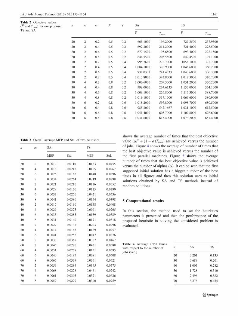
For instance, some typical test problems are selected andsolved, in which each objective function value (i.e., F andTmax) is computed for TS and SA. The related results are shownin Table 2. The objective values convert to the (0, 1) intervalfor gaining a single objective function, aFþ 1� að ÞTmax.

For each generated problem, as performance measures,we compute the efficiency of the proposed heuristics byconsidering two measures: namely mean error percentage(MEP) and standard deviation of errors (Std.). The MEP iscomputed by:

objective value of the best solution� objective value of the heuristic solution

objective value of the best solution

� 100

The related computational experiments are tabulated andshown in graphs; however they are summarized in Tables 3and 4 as well as Figs. 6, 7, 8, and 9. Table 3 presents theMEP and Std. with respect to the number of jobs (n) andamong different numbers of the first stage parallel machines(m). As shown in this table, SA performs better than TS insolving our presented model because the results of themean error percentages achieved by SA are less than TS. Inaddition, there are fewer fluctuations among the jobs in SAthan TS. TS perform worse than SA when the number ofjobs increases.

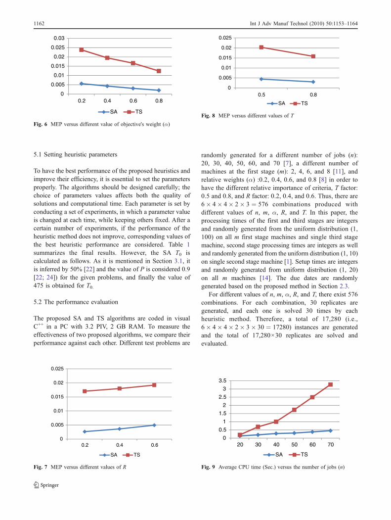
Figure 6 illustrates the MEP through the differentvalue of the weight (α). It is obviously seen that, when αincreases, more weight is given to F criteria and lessweight is given to Tmax. The mean error percentagedecreases when α increases. It should be reminded thatthe SPT rule is used as initial solution for SA and TS. It isknown that the SPT rule is a good heuristic method for F.It can be a reason for decreasing the mean error percen-tage when α increases. Furthermore, SA performs betterthan TS in terms of the performance measure, namelyMEP.

Figures 7 and 8 illustrate the MEP for different values ofR and T, respectively. It is worth noting that the larger valueof R causes the wider spread of due dates among jobs andchanges of T move the interval of due dates. It is importantto monitor the trend of algorithms by changing these twoparameters. As R increases, the MEP of two heuristics getsworse; however, SA has better performance than TS interms of the MEP. By increasing T, the MEP of twoheuristics gets better and SA works better than TS in termsof the MEP. Different compositions of R and T do not affecton the heuristics performances. In our experiments, we findout that SA works better than TS.

The CPU time of the heuristic algorithms are shown inFig. 9 and Table 4. It can be seen that SA consumes lesstime than TS, and both of them become larger for jobs withlarger numbers. Therefore, SA has the best performanceand consumes less time and it can be suggested as a betterheuristic method than TS in the considered problem.

6 Conclusions

In this paper, we have presented a novel three-stageassembly flow shop scheduling problem with sequence-dependent setup times that minimizes the mean flow timeand maximum tardiness. First, the problem was formulatedby using a nonlinear model that is strongly NP-hardness[1], especially for large-sized problems. In addition, an LBmethod has been developed for our new presented model.Furthermore, we have proposed an SA and TS algorithmsto solve the presented problems, and their performances andresults have been compared. Two proposed initial solutionshave been compared as a heuristic's starting point.Moreover, extensive computational experiments have beencarried out in order to evaluate the performance of theproposed SA and TS. The computational results haveshown that the proposed SA outperforms the proposed TS.

Some possible extensions can be considered in thepresented problem with machine breakdown, fuzzy datainput, and capacity limitation or buffer between stages forfuture study. Furthermore, more objectives can be consid-ered in a real model.

References

1. Koulamas C, Kyparisis G (2001) The three-stage assemblyflowshop scheduling problem. Comput Oper Res 28:689–704

2. Potts CN, Sevast'janov SV, Strusevich VA, Van Wassenhove LN,Zwaneveld CM (1995) The two-stage assembly schedulingproblem: complexity and approximation. Oper Res 43:346–355

3. Lee CY, Cheng TCE, Lin BMT (1993) Minimizing the makespanin the 3-machine assembly type flowshop scheduling problem.Manag Sci 39:616–625

4. Tozkapan A, Kirca O, Chung CS (2003) A branch and boundalgorithm to minimize the total weighted flowtime for the two-stage assembly scheduling problem. Comput Oper Res 30:309–320

5. Al-Anzi FS, Allahverdi A (2006) A hybrid tabu search heuristicfor the two-stage assembly scheduling problem. Int J OperResearch 3(2):109–119

6. Allahverdi A, Al-Anzi FS (2006) A PSO and a tabu searchheuristics for the assembly scheduling problem of the two-stagedistributed database application. Comput Oper Res 33(4):1056–1080


7. Al-Anzi FS, Allahverdi A (2007) A self-adaptive differential evolutionheuristic for two stage assembly scheduling problem to minimizemaximum lateness with setup times. Eur J Oper Res 182:80–94

8. Allahverdi A, Al-Anzi FS (2007) The two-stage assembly flow-shop scheduling problem with bicriteria of makespan and meancompletion time. Int J Adv Manuf Technol 37(1):166–177

9. Tavakkoli-Moghaddam R, Safaei N, Sassani F (2009) A memeticalgorithm for the flexible flow line scheduling problem withprocessor blocking. Comput Oper Res 36(2):402–414

10. Gharehgozli AH, Tavakkoli-Moghaddam R, Zaerpour N (2009) Afuzzy mixed-integer goal programming model for a parallelmachine scheduling problem with sequence-dependent setup timesand release dates. Robot Comput-Integr Manuf 25(4–5):853–859

11. Al-Anzi FS, Allahverdi A (2009) Heuristics for a two-stageassembly flowshop with bicriteria of maximum lateness andmakespan. Comput Oper Res 36:2682–2689

12. Loukil T, Teghem J, Tuyttens D (2005) Solving multi-objectiveproduction scheduling problems using metaheuristics. Eur J OperRes 161:42–61

13. Rabadi G, Mollaghasemi M, Anagnostopoulos GC (2004) Abranch-and-bound algorithm for the early/tardy machine schedul-ing problem with a common due date and sequence-dependentsetup time. Comput Oper Res 31:1727–1751

14. Lin S-W, Ying K-C, Lee Z-J (2009) Metaheuristics for schedulinga non-permutation flowline manufacturing cell with sequencedependent family setup times. Comput Oper Res 36(4):1110–1121

15. Manjeshwar PK, Damodaran P, Srihari K (2009) Minimizingmakespan in a flow shop with two batch-processing machines usingsimulated annealing. Robot Comput-Integr Manuf 25(3):667–679

16. Safaei N, Saidi-Mehrabad M, Jabal-Ameli MS (2008) A hybridsimulated annealing for solving an extended model of dynamiccellular manufacturing system. Eur J Oper Res 185(2):563–592

17. Seçkiner SU, Kurt M (2007) A simulated annealing approach tothe solution of job rotation scheduling problems. Appl MathComput 188(1):31–45

18. Coli M, Palazzari P (1996) Real time pipelined system designthrough simulated annealing. J Systems Archit 42(6–7):465–475

19. Lee DH, Cao Z, Meng Q (2007) Scheduling of two-transtainersystems for loading outbound containers in port containerterminals with simulated annealing algorithm. Int J Prod Econ107(1):115–124

20. Michalewicz Z, Fogel DB (2000) How to solve it: modernheurestics. Springer-Verlag, New York

21. Russell SJ, Norving P (1995) Artificial intelligence: a modernapproach. Prentice- Hall, Englewood Cliffs

22. Kirkpatrick S, Gelatt CD Jr, Vecchi MP (1983) Optimization bysimulated annealing. Science 220(4598):671–680

23. Parthasarathy S, Rajendran C (1997) A simulated annealingheuristic for scheduling to minimize mean weighted tardiness ina flowshop with sequence-dependent setup times of jobs—a casestudy. Prod Plan Control 8(5):475–483

24. Suresh RK, Mohanasundaram KM (2006) Pareto archivedsimulated annealing for job shop scheduling with multipleobjectives. Int J Adv Manuf Technol 29:184–196

25. Glover F (1989) Tabu search—part I. ORSA J Comput 1(3):190–206

26. Glover F (1990) Tabu search—part II. ORSA J Comput 2(1):4–3227. Glover F, Laguna M (1997) Tabu search. Kluwer Academic

Publishers28. Rayward-Smith VJ, Osman IH, Reeves CR, Smith GD (eds)

(1996) Modern heuristic search methods. Wiley, Chichester29. Reeves CR (ed) (1993) Modern heuristic techniques for combi-

natorial problems. Blackwell Scientic Publications, Oxford


Documents

Two meta-heuristics for three-stage assembly flowshop scheduling with sequence-dependent setup times