Embed Size (px)
Citation preview
Arnold Math J. (2018) 4:27–57https://doi.org/10.1007/s40598-018-0085-2
RESEARCH EXPOSITION
Two-Valued Groups, Kummer Varieties, and IntegrableBilliards
V. M. Buchstaber1 · V. Dragovic2,3
Received: 10 July 2017 / Revised: 30 November 2017 / Accepted: 10 March 2018 /Published online: 9 April 2018© Institute for Mathematical Sciences (IMS), Stony Brook University, NY 2018
Abstract A natural and important question of study two-valued groups associatedwith hyperelliptic Jacobians and their relationship with integrable systems is moti-vated by seminal examples of relationship between algebraic two-valued groupsrelated to elliptic curves and integrable systems such as elliptic billiards and cele-brated Kowalevski top. The present paper is devoted to the case of genus 2, to theinvestigation of algebraic two-valued group structures on Kummer varieties. One ofour approaches is based on the theory of σ -functions. It enables us to study the depen-dence of parameters of the curves, including rational limits. Following this line, weare introducing a notion of n-groupoid as natural multivalued analogue of the notionof topological groupoid. Our second approach is geometric. It is based on a geomet-ric approach to addition laws on hyperelliptic Jacobians and on a recent notion ofbilliard algebra. Especially important is connection with integrable billiard systemswithin confocal quadrics. The third approach is based on the realization of the Kum-mer variety in the framework of moduli of semi-stable bundles, after Narasimhan andRamanan. This construction of the two-valued structure is remarkably similar to thehistorically first example of topological formal two-valued group from 1971, with asignificant difference: the resulting bundles in the 1971 case were ”virtual”, while inthe present case the resulting bundles are effectively realizable.
B V. [email protected]
V. M. [email protected]
1 Steklov Mathematical Institute, Russian Academy of Sciences, Gubkina Street 8, 119991Moscow, Russia
2 Department of Mathematical Sciences, The University of Texas at Dallas,800 West Campbell Rd, Richardson, TX 75080, USA
3 Mathematical Institute SANU, Belgrade, Serbia
123
28 V. M. Buchstaber, V. Dragovic
Keywords 2-valued groups · Kummer varieties · Hyperelliptic Jacobians · Integrablebilliards · Semi-stable bundles
Mathematics Subject Classification 20N20 · 14H40 · 14H70
Contents
1 Introduction . . . . . . . . . . . . . . . . . . . . . . . . . . . . . . . . . . . . . . . . . . . . . 282 From n-Valued Groups to n-Groupoids . . . . . . . . . . . . . . . . . . . . . . . . . . . . . . . 30
2.1 Defining Notions and Basic Examples of n-Valued Groups . . . . . . . . . . . . . . . . . . 302.2 Topological n-Groupoids . . . . . . . . . . . . . . . . . . . . . . . . . . . . . . . . . . . . 33
3 Rational Limit of a Kummer Surface and Two-Valued Addition Law . . . . . . . . . . . . . . . 353.1 Two-Dimensional Abelian Functions . . . . . . . . . . . . . . . . . . . . . . . . . . . . . . 353.2 Rational Limit Embedding and Two-Valued Group Law . . . . . . . . . . . . . . . . . . . . 363.3 Rational Kummer Two-Valued Group . . . . . . . . . . . . . . . . . . . . . . . . . . . . . 38
4 Two-Valued Group Structures on Kummer Varieties and Sigma-Functions . . . . . . . . . . . . . 405 Homomorphism of Rings of Functions, Induced by Abel Mapping in Genus 2 . . . . . . . . . . 436 Geometric Two-Valued Group Laws and Kummer Varieties . . . . . . . . . . . . . . . . . . . . 45
6.1 A Quadric in CP5 and A Line Complex in CP3 . . . . . . . . . . . . . . . . . . . . . . . . 456.2 Smooth Intersection of Two Quadrics and Abelian Varieties . . . . . . . . . . . . . . . . . . 466.3 Pencils of Quadrics, Hyperelliptic Curves and Geometric Group Laws . . . . . . . . . . . . 48
7 Integrable Billiards and Two-Valued Laws . . . . . . . . . . . . . . . . . . . . . . . . . . . . . 517.1 Pencils of Quadrics and Billiards . . . . . . . . . . . . . . . . . . . . . . . . . . . . . . . . 51
8 Moduli of Semi-Stable Bundles and Two-Valued Group Structure on Kummer Varieties . . . . . 54References . . . . . . . . . . . . . . . . . . . . . . . . . . . . . . . . . . . . . . . . . . . . . . . . 56
1 Introduction
The deep connection between two-valued groups and integrable systems is well-known. In Buchstaber and Veselov (1996), a two-valued action of two-valued groupZ+ has been related to the Euler-Chasles correspondence, as a basis of billiard dynam-ics within conics, as an example of integrable discrete dynamics.
The concept of integrability in context of discrete dynamical systems goes back toVeselov (1992), Moser and Veselov (1991). They established integrability of billiarddynamics generated by pencils of quadrics and related it in case of two-dimensionalquadrics of three-dimensional space with Jacobians of hyperelliptic curves of genus 2.
The aim of this paper is to develop algebraic two-valued group structure on theKummer varieties and to study its relationship with integrable billiard systems withinpencils of quadrics. The Kummer variety is a classical and well-studied object of thealgebraic geometry. It appears as a variety of orbits of a Jacobian of a curve of genus 2,factorized by the hyperelliptic involution. Thus, there are various algebro-geometricand analytical structures on it, related to the moduli of curves of genus 2. We want tounderstand and present the structure of an algebraic two-valued group associated todifferent appearances of the Kummer varieties. Let us mention that from the point ofview of differential geometry and the theory of abelian functions of genus 2, Kummervarieties have been studied by Baker.
One side of our approach is based on the theory of σ -functions. The choice of σ
functions is motivated by our wish to study dependence of parameters of the curves.
123
Two-Valued Groups, Kummer Varieties… 29
As we know from the theory of integrable systems, (see Dubrovin and Novikov 1975),it is important to study not only a single curve and its Jacobian, but rather a whole classof curves and their Jacobians. Following this line, let B denote a set parameterizingnonsingular curves of genus 2 and let U be the analytic bundle over B with a genus2 curve as a fibre. We denote by J (U ) the associated bundle over B with a Jacobianof a genus 2 curve as a fiber. Then, J (U ) has a natural structure of a topologicalgroupoid, see Buchstaber and Leykin (2005). The description of the correspondingassociated bundle over B with a Kummer variety as a fiber was done in Buchstaber(2016).
Higher genera Poncelet type problems, integrable billiards and so-called billiardalgebra associatedwith pencils of quadrics in arbitrary dimensions have been studied inDragovic and Radnovic (2006, 2008), where the relationship with hyperelliptic curvesand their Jacobians has been considered (see also Dragovic and Radnovic 2011).
In the next section, after recalling the definition of the n valued group, we areintroducing a notion of n-groupoid, which enables us to consider not only a singlestructure of a two-valued group, but also dependance of the parameters of the curve.Thus the notion of n-groupoid is a natural analogue of the notion of topologicalgroupoid.
Another important reason of usingσ -functions, lies in the fact that addition relationsfor them are well adjusted to two-valued structure, as one can easily see from the genusone case formula:
σ(u + v)σ (u − v) = σ(u)2σ(v)2(℘(v) − ℘(u)
),
The program of construction of σ -functions of higher genera had been proposedby Klein. In genus 2 case, the program got rather advanced development by Baker(see Baker 1898), although in his last review of the program in 1923, Klein notedthat program for genus g > 2 was still far from being completed. We base our firstapproach on the results fromBuchstaber and Leykin (2005) and references therein. Forsome recent applications to the theory of integrable systems, see Buchstaber (2016)and Buchstaber and Mikhailov (2017).
Our second approach is geometric. Following Donagi (1980), Knörrer (1980),Griffiths and Harris (1994), Audin (1994) a geometric approach to addition laws onhyperelliptic Jacobians has been developed further in Dragovic and Radnovic (2008)(see alsoDragovic andRadnovic 2011). It has been based on the notion of billiard alge-bra and it has been connected to integrable billiard systems within confocal quadrics.
Our first approach is developed in Sect. 4, and the second one in Sect. 6. The study ofthe rational limit of a Kummer surface and related two-valued group law is performedin Sect. 3.
In Sect. 7, the geometric approach from the Sect. 6, develops further toward inte-grable systems, through the integrable billiards and the billiard algebra and ismotivatedby Audin (1994), Dragovic and Radnovic (2008) .
The final Sect. 8 gives yet another construction of the two-valued group law on theKummer variety, based on the realization of the Kummer variety in the framework ofmoduli of semi-stable bundles. This framework has been developed by Narasimhanand Ramanan, see Narasimhan and Ramanan (1969). This last construction of the two-
123
30 V. M. Buchstaber, V. Dragovic
valued structure is remarkably similar to the historically first example of topologicaltwo-valued group from 1971 (see Buchstaber and Novikov 1971), with a significantdifference. The resulting bundles in the 1971 case of Buchstaber and Novikov (1971)are “virtual”, while in the present case the resulting bundles are effectively realizable.
2 From n-Valued Groups to n-Groupoids
The study of structure of multivalued groups has been started in 1971 [see Buchstaberand Novikov (1971)] within the study of characteristic classes of vector bundles, atthat time as the structure of formal (local) multivalued groups. In 1990, in Buchstaber(1990) has been introduced algebraic two-valued group structure on CP1 by usingaddition theorems on elliptic curves. The structure of algebraic multivalued groupshas been studied since then extensively [see Buchstaber (2006) and references therein]in different contexts.
However, it has got a new impetus with a recent paper Dragovic (2010), where aconnection between two-valued groups onCP1 and the celebrated Kowalevski top hasbeen discovered. There, it was shown that the famous, and still not fully understoodKowalevski change of variables [see, for example, Audin (1999)] corresponds to theoperation in two-valued group W/τ , where W is an elliptic curve, in the standardWeierstrass model of elliptic curve, with τ as the canonical involution. More detaileddescription of this two-valued group is presented in Sect. 2.1, see Example 3. Thisdeep connection of the Kowalevski integration procedure with a structure of ellipticcurve, on the first glance, may be in surprising contrast to a well known fact that theintegration of the Kowalevski top is performed on Jacobian of a genus two curve.Moreover, as it has been shown in Dragovic (2010), the Kowalevski integration pro-cedure can be interpreted as a certain deformation of the two-valued group p2 (seeExample 2) toward the structure on W/τ . The structure of p2 is the rational limit ofthe one on W/τ . In addition, in Dragovic (2010) it has been proven the equivalencebetween associativity of the two-valued group on W/τ with the Poncelet theorem ofpencils of conics, in the case of triangles.
2.1 Defining Notions and Basic Examples of n-Valued Groups
We follow Buchstaber (2006) and define an n-valued group on X as a map:
m : X × X → (X)n
m(x, y) = x ∗ y = [z1, . . . , zn].
Here (X)n denotes the symmetric n-th power of X and zi coordinates therein.Associativity is a generalization of the usual condition of associativity and is
expressed as equality of two n2-sets
[x ∗ (y ∗ z)1, . . . , x ∗ (y ∗ z)n][(x ∗ y)1 ∗ z, . . . , (x ∗ y)n ∗ z]
123
Two-Valued Groups, Kummer Varieties… 31
for all triplets (x, y, z) ∈ X3. An element e ∈ X is a unit if
e ∗ x = x ∗ e = [x, . . . , x],
for all x ∈ X . Similarly, a map inv : X → X is an inverse if it satisfies
e ∈ inv(x) ∗ x, e ∈ x ∗ inv(x),
for all x ∈ X .As in Buchstaber (2006), m determines an n-valued group structure (X,m, e, inv)
if it is associative, with a unit and with an inverse. Naturally, an n-valued group X actson the set Y if there is a mapping
φ : X × Y → (Y )n
φ(x, y) = x ◦ y,
such that the two n2-multisubsets of Y
x1 ◦ (x2 ◦ y) (x1 ∗ x2) ◦ y
are equal for all x1, x2 ∈ X, y ∈ Y . It is additionally required that
e ◦ y = [y, . . . , y]
for all y ∈ Y .
Example 1 [A two-valued group structure on Z+, Buchstaber and Veselov (1996)]Let us consider the set of nonnegative integers Z+ and define a mapping
m : Z+ × Z+ → (Z+)2,
m(x, y) = [x + y, |x − y|].
This mapping provides a structure of a two-valued group on Z+ with the unit e = 0and the inverse equal to the identity inv(x) = x .
In Buchstaber and Veselov (1996) sequence of two-valued mappings associatedwith the Poncelet porism was identified as the algebraic representation of this 2-valued group. Moreover, the algebraic action of this group on CP1 was studied and itwas shown that in the irreducible case all such actions are generated by Euler-Chaslescorrespondences.
Example 2 [2-valued group on (C,+)] Among the basic examples of multivaluedgroups, there are n-valued additive group structures on C. For n = 2, this is a two-valued group p2 defined by the relation
m2 : C × C → (C)2
x ∗2 y = [(√x + √y)2, (
√x − √
y)2] (1)
123
32 V. M. Buchstaber, V. Dragovic
The product x ∗2 y corresponds to the roots in z of the polynomial equation
p2(z, x, y) = 0,
where
p2(z, x, y) = (x + y + z)2 − 4(xy + yz + zx).
This two-valued group structure has been connected with degenerations of theKowalevski top in Dragovic (2010). Similar integrable systems were studied byAppel’rot, Delone, Mlodzeevskii [see Golubev 1960 and references therein.]
As it has been observed in Dragovic (2010), the general Kowalevski case is con-nected with p2 together with its deformation on CP1 as a factor of an elliptic curve,see the next example.
Example 3 [2-valued group on S2 = C, associated with an elliptic curve] Supposethat a cubic W is given in the standard form
W : t2 = J (s) = 4s3 − g2s − g3.
Consider the mappingW → S2 = C : (s, t) �→ s, where C represents a complex lineextended by ∞.
The curve W as a cubic curve has the group structure. Together with its canonicalinvolution τ : (s, t) �→ (s,−t), it defines the standard two-valued group structure ofcoset type (see Buchstaber and Rees 2002; Buchstaber 2006) on S2 with the unit atinfinity in S2. The product is defined by the formula:
[s1] ∗c [s2] =[[
−s1 − s2 +(
t1 − t22(s1 − s2)
)2]
,
[
−s1 − s2 +(
t1 + t22(s1 − s2)
)2]]
,
(2)where ti = J (si ), i = 1, 2, and
[si ] = {(si , ti ), (si ,−ti )}, si = ℘(ui ), ti = ℘′(ui ),
by using addition theorem for the Weierstrass function ℘(u):
℘(u1 + u2) = −℘(u1) − ℘(u2) +(
℘′(u1) − ℘′(u2)2(℘ (u1) − ℘(u2))
)2
.
The Kowalevski integration procedure was explained in Dragovic (2010) as certaindeformation of p2 to (W, τ ) [see also Dragovic and Kukic (2014a, b, c), Dragovic andGajic (2016) for further developments].
The 2-group structure (W, τ ) is also connected with the Poncelet and the Darbouxtheorem [see Darboux 1917; Dragovic 2009; Dragovic and Radnovic 2008].
In this example, g2, g3 are parameters of the curve, and they lead to a rational limit,in the standard limit procedure.
123
Two-Valued Groups, Kummer Varieties… 33
Example 4 Let X be a topological space. Denote byW (X) the set of all 2-dimensionalcomplex vector bundles ζ = η + η over X , where η is a linear complex vector bundleover X . Then the formula
ζ1 ⊗ ζ2 = (η1 ⊗ η2 + η1 ⊗ η2) + (η1 ⊗ η2 + η1 ⊗ η2)
gives the structure of a 2-valued group on W (X) defined by the 2-valued multipli-cation
ζ1 � ζ2 = [(η1 ⊗ η2 + η1 ⊗ η2), (η1 ⊗ η2 + η1 ⊗ η2)].
2.2 Topological n-Groupoids
Following Buchstaber and Leykin (2005), let us fix a topological space Y . A space Xwith a map pX : X → Y is called a space over Y , and the map pX is called anchor.For Y , the anchor pY is the identity map.
Amap f : X1 → X2 of two spaces over Y is called a map over Y if pX2 ◦ f = pX1 .For two spaces X1, X2 over Y , their direct product over Y is defined as
X1 ×Y X2 = {(x1, x2) ∈ X1 × X2 | pX1(x1) = pX2(x2)}
with the map pX1×Y X2(x1, x2) = pX1(x1). Along this line, one may define a productover Y of n spaces X1, . . . Xn over Y
X1 ×Y · · · ×Y Xn = {(x1, . . . , xn) ∈ X1 × X2 × · · · × Xn | pX1(x1)
= pX2(x2) = · · · = pXn (xn)}.
In a special case X1 = · · · = Xn = X , we define n-th power of X over Y and denoteit as Xn
Y .For a space X over Y we define its n-th symmetric power over Y , denoted as
(X)nY
as the quotient of XnY by the action of the permutation group.
We define also the diagonal map over Y
D : X → (X)nY , x �→ (x, x, . . . , x).
Definition 1 A space X with an anchor pX : X → Y and structural maps over Y :
μ : X ×Y X → (X)nY , inv : X → X, e : Y → X
is called an n-groupoid over Y if the following conditions are satisfied:
123
34 V. M. Buchstaber, V. Dragovic
(1) For x1, x2, x3 such that pX (x1) = pX (x2) = pX (x3): if
μ(x1, x2) = [z1, . . . , zn], μ(x2, x3) = [w1, . . . , wn],
then
[μ(x1, w1), . . . , μ(x1, wn)] = [μ(z1, x3), . . . , μ(zn, x3)].
(2) For every x ∈ X and y = pX (x) ∈ Y :
μ(e(y), x) = μ(x, e(y)) = D(x).
(3) For every x ∈ X and y = pX (x) ∈ Y :
e(y) ∈ μ(x, inv(x)), e(y) ∈ μ(inv(x), x).
Example 5 Let X = C × C, Y = C and an anchor is defined as the projection to thesecond component
pX := p2 : X → Y, pX (x, λ) := λ.
We define a 2-groupoid over Y starting with an operation over Y
A((x1, λ), (x2, λ)) = (x1 + x2 − λx1x2, λ).
An involutive automorphism I over Y is defined by
I : X → X, (u, λ) =(
− u
1 − λu, λ
).
If we denote by uu = x, vv = y, then the 2-groupoid over Y is defined by
μ((x, λ), (y, λ)) = [(z1, λ), (z2, λ)]
where zi , i = 1, 2 are solutions of the following quadratic equation
Z2 −(2(x + y) − λ2xy
)Z + (x − y)2 = 0.
Notice that we get p2 for λ = 0. Thus the structure of the above 2-groupoid is certaindeformation of p2.
123
Two-Valued Groups, Kummer Varieties… 35
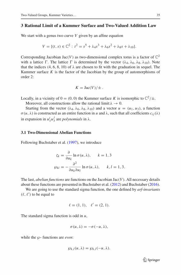
3 Rational Limit of a Kummer Surface and Two-Valued Addition Law
We start with a genus two curve V given by an affine equation
V = {(t, s) ∈ C2 : t2 = s5 + λ4s
3 + λ6s2 + λ8s + λ10}.
Corresponding Jacobian Jac(V ) as two-dimensional complex torus is a factor of C2
with a lattice . The lattice is determined by the vector (λ4, λ6, λ8, λ10). Notethat the indices (4, 6, 8, 10) of λ are chosen to fit with the graduation in sequel. TheKummer surface K is the factor of the Jacobian by the group of automorphisms oforder 2:
K = Jac(V )/± .
Locally, in a vicinity of 0 = (0, 0) the Kummer surface K is isomorphic to C2/±.Moreover, all constructions allow the rational limit:λ → 0.Starting from the vector (λ4, λ6, λ8, λ10) and a vector u = (u1, u3), a function
σ(u, λ) is constructed as an entire function in u and λ, such that all coefficients ci j (λ)
in expansion in ui1uj3 are polynomials in λ.
3.1 Two-Dimensional Abelian Functions
Following Buchstaber et al. (1997), we introduce
ζk = ∂
∂ukln σ(u, λ), k = 1, 3
℘kl = − ∂2
∂uk∂ulln σ(u, λ), k, l = 1, 3.
The last, abelian functions are functions on the Jacobian Jac(V ). All necessary detailsabout these functions are presented in Buchstaber et al. (2012) and Buchstaber (2016).
We are going to use the standard sigma function, the one defined by arf-invariants(�, �′) to be equal to
� = (1, 1), �′ = (2, 1).
The standard sigma function is odd in u,
σ(u, λ) = −σ(−u, λ),
while the ℘- functions are even:
℘k,l(u, λ) = ℘k,l(−u, λ).
123
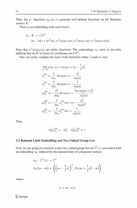
36 V. M. Buchstaber, V. Dragovic
Thus, the ℘- functions ℘k,l(u, λ) generate well-defined functions on the Kummersurface K .
There is an embedding with each fixed λ:
πλ : K → CP3
[u,−u] �→ [σ 2(u), σ 2(u)℘11(u), σ 2(u)℘13(u), σ 2(u)℘33(u)].
Note that σ 2(u)℘kl(u) are entire functions. The embeddings πλ serve to describeaddition law on K in terms of coordinates on CP3.
One can easily compute the limit of the functions when λ tends to zero:
limλ→0
σ(u, λ) = σ0(u) = u3 − 1
3u31
ζ(0)1 = ∂
∂u1ln σ0(u) = − u21
σ0(u)
ζ(0)3 = ∂
∂u3ln σ0(u) = − 1
σ0(u)
℘(0)11 = − ∂2
∂u21ln σ0(u) = 2u1σ0(u) + u41
σ 20 (u)
℘(0)13 = − ∂
∂u1ζ
(0)3 (u) == − u21
σ0(u)2
℘(0)33 = − ∂
∂u3ζ
(0)3 (u) = 1
σ 20 (u)
.
Thus,
σ 20 ℘
(0)13 = −u21, σ 2
0 ℘(0)33 = 1.
3.2 Rational Limit Embedding and Two-Valued Group Law
Now, we are going to construct a new two-valued group law onC2/± associated withan embedding πK induced by the rational limit of a Kummer surface:
πK : C2/± → C
3
πK ([u,−u]) =((
u3 − 1
3u31
)2
, 2u1u3 + 1
3u41,−u21
)
,
where
u = (u1, u3).
123
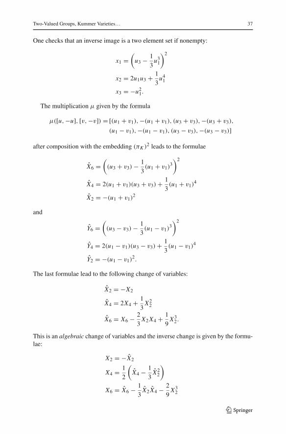
Two-Valued Groups, Kummer Varieties… 37
One checks that an inverse image is a two element set if nonempty:
x1 =(u3 − 1
3u31
)2
x2 = 2u1u3 + 1
3u41
x3 = −u21.
The multiplication μ given by the formula
μ([u,−u], [v,−v]) = [(u1 + v1),−(u1 + v1), (u3 + v3),−(u3 + v3),
(u1 − v1),−(u1 − v1), (u3 − v3),−(u3 − v3)]
after composition with the embedding (πK )2 leads to the formulae
X6 =(
(u3 + v3) − 1
3(u1 + v1)
3)2
X4 = 2(u1 + v1)(u3 + v3) + 1
3(u1 + v1)
4
X2 = −(u1 + v1)2
and
Y6 =(
(u3 − v3) − 1
3(u1 − v1)
3)2
Y4 = 2(u1 − v1)(u3 − v3) + 1
3(u1 − v1)
4
Y2 = −(u1 − v1)2.
The last formulae lead to the following change of variables:
X2 = −X2
X4 = 2X4 + 1
3X22
X6 = X6 − 2
3X2X4 + 1
9X32.
This is an algebraic change of variables and the inverse change is given by the formu-lae:
X2 = −X2
X4 = 1
2
(X4 − 1
3X22
)
X6 = X6 − 1
3X2 X4 − 2
9X32
123
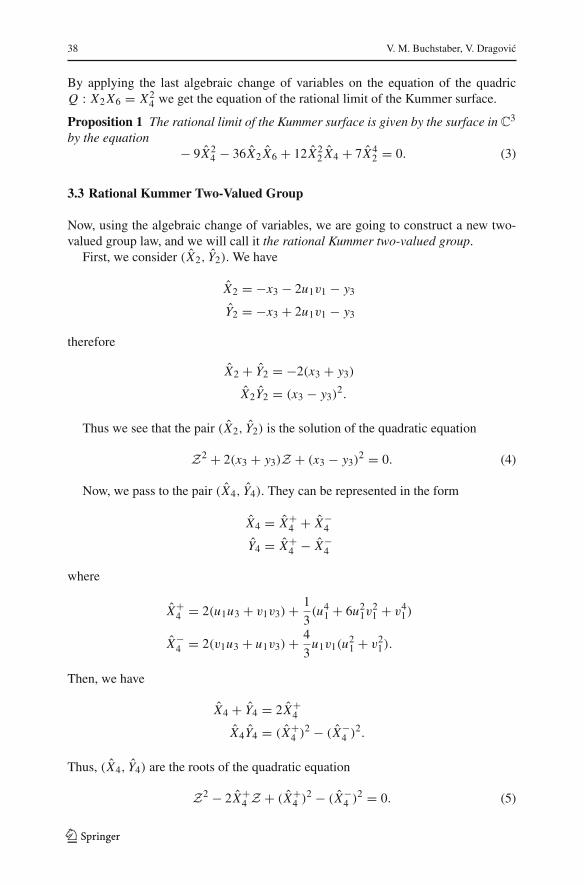
38 V. M. Buchstaber, V. Dragovic
By applying the last algebraic change of variables on the equation of the quadricQ : X2X6 = X2
4 we get the equation of the rational limit of the Kummer surface.
Proposition 1 The rational limit of the Kummer surface is given by the surface in C3
by the equation− 9X2
4 − 36X2 X6 + 12X22 X4 + 7X4
2 = 0. (3)
3.3 Rational Kummer Two-Valued Group
Now, using the algebraic change of variables, we are going to construct a new two-valued group law, and we will call it the rational Kummer two-valued group.
First, we consider (X2, Y2). We have
X2 = −x3 − 2u1v1 − y3
Y2 = −x3 + 2u1v1 − y3
therefore
X2 + Y2 = −2(x3 + y3)
X2Y2 = (x3 − y3)2.
Thus we see that the pair (X2, Y2) is the solution of the quadratic equation
Z2 + 2(x3 + y3)Z + (x3 − y3)2 = 0. (4)
Now, we pass to the pair (X4, Y4). They can be represented in the form
X4 = X+4 + X−
4
Y4 = X+4 − X−
4
where
X+4 = 2(u1u3 + v1v3) + 1
3(u41 + 6u21v
21 + v41)
X−4 = 2(v1u3 + u1v3) + 4
3u1v1(u
21 + v21).
Then, we have
X4 + Y4 = 2X+4
X4Y4 = (X+4 )2 − (X−
4 )2.
Thus, (X4, Y4) are the roots of the quadratic equation
Z2 − 2X+4 Z + (X+
4 )2 − (X−4 )2 = 0. (5)
123
Two-Valued Groups, Kummer Varieties… 39
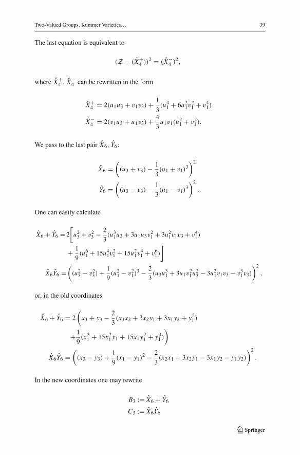
The last equation is equivalent to
(Z − (X+4 ))2 = (X−
4 )2,
where X+4 , X−
4 can be rewritten in the form
X+4 = 2(u1u3 + v1v3) + 1
3(u41 + 6u21v
21 + v41)
X−4 = 2(v1u3 + u1v3) + 4
3u1v1(u
21 + v21).
We pass to the last pair X6, Y6:
X6 =(
(u3 + v3) − 1
3(u1 + v1)
3)2
Y6 =(
(u3 − v3) − 1
3(u1 − v1)
3)2
.
One can easily calculate
X6 + Y6 = 2
[u23 + v23 − 2
3(u31u3 + 3u1u3v
21 + 3u21v1v3 + v41)
+ 1
9(u61 + 15u41v
21 + 15u21v
41 + v61)
]
X6Y6 =(
(u23 − v23) + 1
9(u21 − v21)
3 − 2
3(u3u
31 + 3u1v
21u
23 − 3u21v1v3 − v31v3)
)2
,
or, in the old coordinates
X6 + Y6 = 2
(x3 + y3 − 2
3(x3x2 + 3x2y1 + 3x1y2 + y21 )
+1
9(x31 + 15x21 y1 + 15x1y
21 + y31)
)
X6Y6 =(
(x3 − y3) + 1
9(x1 − y1)
2 − 2
3(x2x1 + 3x2y1 − 3x1y2 − y1y2)
)2
.
In the new coordinates one may rewrite
B3 := X6 + Y6
C3 := X6Y6
123
40 V. M. Buchstaber, V. Dragovic
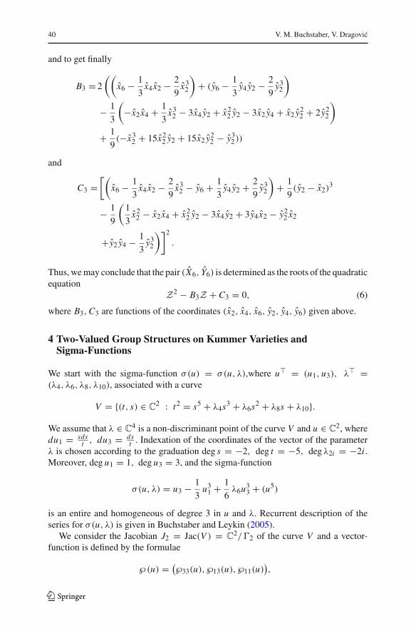
and to get finally
B3 = 2
((x6 − 1
3x4 x2 − 2
9x32
)+ (y6 − 1
3y4 y2 − 2
9y32
)
− 1
3
(−x2 x4 + 1
3x32 − 3x4 y2 + x22 y2 − 3x2 y4 + x2 y
22 + 2 y22
)
+ 1
9(−x32 + 15x22 y2 + 15x2 y
22 − y32))
and
C3 =[(
x6 − 1
3x4 x2 − 2
9x32 − y6 + 1
3y4 y2 + 2
9y32
)+ 1
9(y2 − x2)
3
− 1
9
(1
3x22 − x2 x4 + x22 y2 − 3x4 y2 + 3y4 x2 − y22 x2
+y2 y4 − 1
3y32
)]2.
Thus,wemay conclude that the pair (X6, Y6) is determined as the roots of the quadraticequation
Z2 − B3Z + C3 = 0, (6)
where B3,C3 are functions of the coordinates (x2, x4, x6, y2, y4, y6) given above.
4 Two-Valued Group Structures on Kummer Varieties andSigma-Functions
We start with the sigma-function σ(u) = σ(u, λ),where u� = (u1, u3), λ� =(λ4, λ6, λ8, λ10), associated with a curve
V = {(t, s) ∈ C2 : t2 = s5 + λ4s
3 + λ6s2 + λ8s + λ10}.
We assume that λ ∈ C4 is a non-discriminant point of the curve V and u ∈ C
2, wheredu1 = sds
t , du3 = dst . Indexation of the coordinates of the vector of the parameter
λ is chosen according to the graduation deg s = −2, deg t = −5, deg λ2i = −2i .Moreover, deg u1 = 1, deg u3 = 3, and the sigma-function
σ(u, λ) = u3 − 1
3u31 + 1
6λ6u
33 + (u5)
is an entire and homogeneous of degree 3 in u and λ. Recurrent description of theseries for σ(u, λ) is given in Buchstaber and Leykin (2005).
We consider the Jacobian J2 = Jac(V ) = C2/2 of the curve V and a vector-
function is defined by the formulae
℘(u) = (℘33(u), ℘13(u), ℘11(u)
),
123
Two-Valued Groups, Kummer Varieties… 41
where ℘kl(u) = − ∂2
∂uk∂ulln σ(u), k, l = 1, 3. Since the function σ(u) is odd, we get
a mapping
i : J2 −→ CP3 : i(u) = (x0 : x2 : x4 : x6),
where x0 = σ(u)2℘33(u), x2 = σ(u)2℘13(u), x4 = σ(u)2℘11(u), x6 = σ(u)2.The last mapping factorizes through the Kummer variety K together with an embed-ding
i : K = (J2/±) −→ CP3.
Let us note, that the embedding i is defined with entire homogeneous functionsx2k(u), deg x2k = 2k, k = 0, . . . , 3.
We are going to use a ramified covering
γ : (CP3)2 −→ CP6,
defined by the relation
[p(x, t), p(y, t)] −→ p(x, t)p(y, t),
where p(x, t) = x0t33 + x2t23 t1 + x4t3t21 + x6t31 . By putting deg tk = k, we get p(x, t)as a homogeneous polynomial of degree 9.
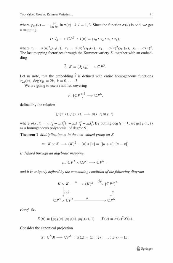
Theorem 1 Multiplication m in the two-valued group on K
m : K × K −→ (K )2 : [u] ∗ [u] = ([u + v], [u − v])
is defined through an algebraic mapping
μ : CP3 × CP3 −→ CP6 :
and it is uniquely defined by the commuting condition of the following diagram
K × Km
i×i
(K )2(i)2 (
CP3)2
γ
CP3 × CP3 μCP6
Proof Set
X (u) = (℘33(u), ℘31(u), ℘11(u), 1
) X (u) = σ(u)2X (u).
Consider the canonical projection
π : C7\0 −→ CP6 : π(z) = (z0 : z2 : . . . : z12) = [z].
123
42 V. M. Buchstaber, V. Dragovic
According to the construction, we have
i [u] = [X (u)] , γ ( i )2([u] ∗ [v]) = γ
([X (u + v),X (u − v)]
).
Thus, we have to show that each coordinate z2k(u, v), k = 0, . . . , 6, of the pointγ([X (u + v),X (u − v)]
)is a polynomial of the coordinates x2i , y2i , i = 0, . . . , 3
of the points X (u) X (v).Genus two sigma-function σ(u) satisfies the following addition theorem (see Buch-
staber et al. 1997; Buchstaber and Leykin 2005):
σ(u + v)σ (u − v) = X (u)�J X (v).
where J =(0 −EE 0
)and E =
(0 11 0
). We have,
z12 = z12(u, v) = (X (u)�J X (v))2
.
Thus, we get that in the mapping μ(x, y) = [z] = (z0 : z2 : . . . : z12) ∈ CP6, thecoordinate z12 is defined by the formula z12 = (x�J y)2, where (x, y) ∈ CP3×CP3.
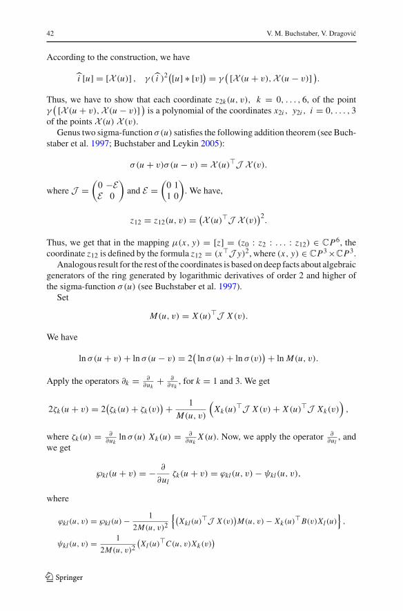
Analogous result for the rest of the coordinates is based ondeep facts about algebraicgenerators of the ring generated by logarithmic derivatives of order 2 and higher ofthe sigma-function σ(u) (see Buchstaber et al. 1997).
Set
M(u, v) = X (u)�J X (v).
We have
ln σ(u + v) + ln σ(u − v) = 2(ln σ(u) + ln σ(v)
) + lnM(u, v).
Apply the operators ∂k = ∂∂uk
+ ∂∂vk
, for k = 1 and 3. We get
2ζk(u + v) = 2(ζk(u) + ζk(v)
) + 1
M(u, v)
(Xk(u)�J X (v) + X (u)�J Xk(v)
),
where ζk(u) = ∂∂uk
ln σ(u) Xk(u) = ∂∂uk
X (u). Now, we apply the operator ∂∂ul
, andwe get
℘kl(u + v) = − ∂
∂ulζk(u + v) = ϕkl(u, v) − ψkl(u, v),
where
ϕkl (u, v) = ℘kl (u) − 1
2M(u, v)2
{(Xkl (u)�J X (v)
)M(u, v) − Xk(u)�B(v)Xl (u)
},
ψkl (u, v) = 1
2M(u, v)2
(Xl (u)�C(u, v)Xk(v)
)
123
Two-Valued Groups, Kummer Varieties… 43
and B(v) = J X (v)X (v)�J �, C(u, v) = (M(u, v) − J X (v)X (u)�
)J .Note B(−v) = B(v) C(−u, v) = C(u,−v) = C(u, v). Thus, ϕkl(u,−v) =
ϕkl(u, v) ψkl(u,−v) = −ψkl(u, v). We get
X (u + v) = σ(u + v)2(X1 − X2) X (u − v) = σ(u − v)2(X1 + X2),
where X1 = (ϕ33, ϕ13, ϕ11, 1) X2 = (ψ33, ψ13, ψ11, 0). We obtain
p(X (u + v), t
)p(X (u − v), t
) = z1 · (p(X1, t)
2 − p(X2, t)2)
where
p(X1, t) = ϕ33t33 + ϕ13t
23 t1 + ϕ11t3t
21 + t31 ,
p(X2, t) = t3(ψ33t23 + ψ13t3t1 + ψ11t
21 ).
From the above formulae for ϕkl(u, v) ψkl(u, v)ψpq(u, v), it immediately fol-lows that these functions are polynomials of ℘i j (u), ℘i jk(u)℘i ′ j ′k′(u), ℘i j pq(u)
℘i j (v), ℘i jk(v)℘i ′ j ′k′(v), ℘i j pq(v). The functions ℘i jk(u)℘i ′ j ′k′(u) ℘i j pq(u), wherei, j, k, i ′, j ′, k′, p, q take values 1 or 3 independently, are polynomials of ℘i j (u) (seeBuchstaber et al. 1997). Consequently, using (x, y)|i×i = (X (u),X (v)
), we get coor-
dinates z2k of the vector μ(x, y) as polynomials of the coordinates of the vectors xand y. �
5 Homomorphism of Rings of Functions, Induced by Abel Mapping inGenus 2
Let V = {(s, μ) ∈ C
2 : μ2 = s5 + λ4s3 + λ6s2 + λ8s + λ10}denotes a hyperellip-
tic curve.
Theorem 2 The Abel mapping
A : (V )2 −→ JacV
induces a homomorphism of rings of functions
A∗ : F(JacV ) −→ F((V )2
)
such that
A∗(℘11(u)) = s1 + s2, A∗(℘13(u)) = −s1s2, A∗(℘33(u)) = F(s1, s2) − 2μ1μ2
(s1 − s2)2,
123
44 V. M. Buchstaber, V. Dragovic
where
F(s1, s2) = 2λ10 + λ8(s1 + s2) + s1s2(2λ6 + λ4(s1 + s2)
),
℘111(u) = 2μ1 − μ2
s1 − s2, ℘113(u) = 2
s1μ2 − s2μ1
s1 − s2
℘331(u) = −2s21μ2 − s22μ1
s1 − s2, ℘333(u) = 2
ψ(s1, s2)μ2 − ψ(s2, s1)μ1
(s1 − s2)3,
and
ψ(s1, s2) = 4λ10 + λ8(3s1 + s2) + 2λ6s1(s1 + s2) + λ4s21 (s1 + 3s2) + s31s2(3s1 + s2).
The proof of the Theorem can be found in Buchstaber et al. (1997). Let us note thatwe use the indexation here different from Buchstaber et al. (1997), in correspondencewith the graduation:
deg s = −2; degμ = −5; deg λ2k = −2k; k = 2, 3, 4, 5; deg ui = i, i = 1, 3.
This provides additional opportunity to check the formulae. Observe that deg℘kl(u) =−(k + l), deg℘klp(u) = −(k + l + p).
Any Abelian function on JacV represents a linear function of ℘111(u) with coef-ficients which are rational functions of ℘11(u) and ℘13(u). On the other hand, fromthe theory of polysymmetric functions (see Gelfand et al. 1994 and Buchstaber andRees 2002), it is known that the field of rational functions on (C2)2 in the coordinates[(s1, μ1), (s2, μ2)] is generated by polysymmetric functions
e10 = s1 + s2, e20 = s1s2, e01 = μ1 + μ2, e02 = μ1μ2, e11 = s1μ2 + s2μ1,
which are related by unique (for (C2)2) relation
(e210 − 4e20
) (e201 − 4e02
)= (e10e01 − 2e11) .
ThemappingA is a birational equivalence, thusA∗ induces isomorphismof thefieldof Abelian functions F(JacV ) on JacV with the field of rational functions F (
(V )2)
on (V )2. We have:
A∗(℘11(u)) = e10, A∗(℘13(u)) = −e20, A∗(℘111(u)) = e10e01 − 2e11e210 − 4e20
.
In this way, the Theorem 2 completely describes the isomorphismA∗ and gives anopportunity to express explicitly, for example, the even functions ℘klp(u)℘k′l ′ p′(u) aspolynomials of ℘kl(u). The explicit formulae for those polynomials are given in thebook Buchstaber et al. (1997).
123
Two-Valued Groups, Kummer Varieties… 45
The hyperelliptic involution acts on (V )2 according to the formula
[(s1, μ1), (s2, μ2)] −→ [(s1,−μ1), (s2,−μ2)] .
TheAbelmapping is invariantwith respect to this involution on (V )2 and the involutionu → −u on JacV .
From the above formulae one can see that the images of the functions ℘kl(u) and℘klp(u)℘k′l ′ p′(u) are even, while the images of the functions ℘klp(u) are odd. Thus,the mapping
A : (V )2/± −→ K = (JacV )/±,
is defined and it induces a homomorphism between rings of functions.There is an addition law on (V )2, with the Abel mapping A as a homomor-
phism. Explicit form of this operation in the coordinates [(s1, μ1), (s2, μ2)] has beendescribed in Buchstaber and Leykin (2005).
Thus, on (V )2/± there is corresponding two-valued addition, such that A is ahomomorphismwith respect to the two-valued group structure on the Kummer varietyK , defined above.
6 Geometric Two-Valued Group Laws and Kummer Varieties
6.1 A Quadric in CP5 and A Line Complex in CP3
Following classics, see Donagi (1980) and references therein, let us consider athree-dimensional projective space CP3 = P(C4) and corresponding GrassmannianGr(2, 4) of all lines in CP3. By Plücker embedding, the Grassmannian Gr(2, 4) canbe realized as a quadric G in CP5 = P(∧2V ), where V = C
4:
Gr(2, 4) ↪→ CP5
� = � < v1, v2 > �→ v1 ∧ v2, v1, v2 ∈ V 4.
The quadric G parameterizes all decomposable elementsw = v1 ∧v2 of P(∧2V ) andthe quadric is described by the Plücker quadratic relation:
G : w ∧ w = 0.
For a given element x ∈ G, denote by �x the line in CP3 which maps to x by theabove embedding.
We consider so-called Schubert cycles:
σ1(�) = {x ∈ G | �x ∩ � �= ∅}σ2(p) = {x ∈ G | �x � p}
σ1,1(h) = {x ∈ G | �x ⊂ h}σ2,1(p, h) = {x ∈ G | p ∈ �x ⊂ h}.
123
46 V. M. Buchstaber, V. Dragovic
One can easily see that every cycle σ1(�) is a hyperplane section of the quadricG. If the line � ∈ CP3 is determined by vectors v1, v2 ∈ V 4 then the hyperplane ofintersection is of the form Hv1∧v2 = {w | w ∧ v1 ∧ v2 = 0}.
Every cycle σ2,1(p, h) is a line in CP5. Every line L ⊂ G is of the form L =σ2,1(p, h).
A line L ⊂ G is a pencil of lines inCP3. This is a confocal pencil with the commonpoint, the focus p ∈ CP3. At the same time this pencil is coplanar with the commonplane h ∈ CP3∗.
Every cycle of the form σ2(p) or of the form σ1,1(h) is a two-plane in CP5.Conversely, every two-plane in G is of the form σ2(p) or of the form σ1,1(h).
Let us recall some general properties of a quadric Q in CPm . The rank of thequadric is equal to the rank of any of its symmetric (m + 1) × (m + 1) matrices. Thequadric is smooth if its rank is maximal, i.e. if rank of Q is m + 1. If the rank of Q isr then it is a cone over a smooth quadric in CPr−1 with a vertex CPm−r . Quadrics ofrank m + 1 and m are called general.
Now, we give a number of well-known facts for the case of a smooth quadric inCP5, see Tyurin (1975), Donagi (1980) and references therein.
Proposition 2 Let G be a smooth quadric in CP5. Then:
(a) There exists a four-dimensional vector space V 4 such that G is the Plücker embed-ding of the Grassmannian of lines in P(V 4).
(b) The maximal linear subspaces of G are two-dimensional and they are of the formσ2(p) or of the form σ1,1(h), where p ∈ CP3 = P(V 4) and h ∈ CP3∗.
(c) The variety C(Q) of all two-dimensional subspaces of G is three-dimensionaland it has two irreducible components, A and B:
A = {σ2(p) | p ∈ CP3 = P(V 4)}B = {σ1,1(h) | h ∈ CP3∗}.
6.2 Smooth Intersection of Two Quadrics and Abelian Varieties
Now we consider the intersection X of two quadrics G and F in CP5. Such a set isclassically called a quadratic complex of lines, if G is understood as a Grassmannianof lines in some CP3. Together with two quadrics G and F , one may consider thewhole pencil of quadrics:
Fλ := F + λG,
and X is the base set for the pencil, the common intersection of quadrics from thepencil, see Tyurin (1975), Donagi (1980) and references therein.
A pencil of quadrics is generic if associated pencil of 6 × 6 symmetric matricescontains six different singular matrices. For a generic pencil Fλ denote by λ1, . . . , λ6the corresponding values of the pencil parameter associatedwith the singular matrices.
123
Two-Valued Groups, Kummer Varieties… 47
The condition that X is smooth is equivalent to the condition that the pencil Fλ isgeneric. Smoothness of X is also equivalent to the fact that all quadrics Fλ are generaland that exactly six of them, Fλ1 , . . . , Fλ6 are singular.
Proposition 3 Suppose X is a smooth intersection of two quadrics X = G ∩ F inCP5. Then:
(a) The maximal linear subspaces of X are one-dimensional.(b) There is a maximal linear subspace through each point of X.(c) There are four maximal linear subspaces passing through a generic point of X.
Given a smooth intersection of quadrics X = G∩F inCP5, followingNarasimhan,Ramanan, Reid andDonagi, seeDonagi (1980) and references there in, in particularM.Reid’s unpublished Cambridge 1972 thesis, let us consider the set of one-dimensionallinear subspaces
A(X) = {L | L ⊂ X, L ∈ Gr(2, 6)}.
Suppose G is realized as a Grassmannian of lines in some CP3, and denote as beforethe two components of C(G) of two-dimensional linear subspaces of G as
A = {σ2(p) | p ∈ CP3 = P(V 4)}B = {σ1,1(h) | h ∈ P
3∗}.
Lemma 1 Given L ∈ A(X). Then:
(a) There is a unique two-dimensional linear subspace of G, σ2(p) ∈ A such thatL ⊂ σ2(p). There is a unique one-dimensional linear subspace of X
L1 ∈ A(X),
such that
σ2(p) ∩ F = L ∪ L1.
(b) There is a unique two-dimensional linear subspace of G, σ1,1(h) ∈ A such thatL ⊂ σ1,1(h). There is a unique one-dimensional linear subspace of X
L2 ∈ A(X),
such that
σ1,1(h) ∩ F = L ∪ L2.
The last Lemma introduces two involutions
i1 :A(X) → A(X), i1 : L �→ L1
i2 :A(X) → A(X), i2 : L �→ L2.
123
48 V. M. Buchstaber, V. Dragovic
As pencils of lines in CP3 the subspaces L and L1 are confocal, they have the samefocus p. In the same manner, the subspaces L and L2 are coplanar, they have the sameplane h.
Moreover, there are two mappings
k1 :A(X) → CP3, k1 : L �→ p
k2 :A(X) → CP3∗, k2 : L �→ h.
The mapping k1 maps a pencil L to its focus in CP3 while k2 maps a pencil to itsplane in CP3∗.
Denote by K ⊂ CP3 the image ofA(X) by k1. We see that k1 is a double coveringofA(X) over K and that the involution i1 interchanges the leaves of the covering. Weare going to call K the Kummer variety of A(X). It is associated to the choice of aquadric G from the pencil and to the choice of a connected component A of C(G).
Similarly, denote by K ∗ ⊂ CP3∗ the image of A(X) by k2. The mapping k2 is adouble covering of A(X) over K and the involution i2 interchanges the leaves of thecovering.We are going to call K ∗ the dual Kummer variety ofA(X). It is associated tothe choice of a quadric G from the pencil and to the choice of a connected componentB of C(G).
It can be shown that K ∗ is dual to K , which means that every plane from K ∗ istangent to K . From the previous considerations it can also be seen that the degree ofK is equal to 4.
For a general point p ∈ CP3 the plane σ2(p) ⊂ G intersects F along a smoothconic. The Kummer variety K coincides with the Kummer variety associated with thequadratic line complex X = G ∪ F , as defined in Griffiths and Harris (1994), Ch. 6.2:the set of the points p ∈ CP3 for which this intersection is a conicwhich is not smooth.For a general point of K this intersection is a degenerate conic which is a union oftwo different lines L and i1(L). But, there is a subset R ⊂ K of sixteen points, forwhich this intersection is a degenerate conic of double line. These sixteen points fromR correspond to the fixed points of the involution i1 and to the ramification points ofthe double covering. We also denote R∗ ⊂ K ∗ the set of points that correspond to thefixed points of the involution i2.
6.3 Pencils of Quadrics, Hyperelliptic Curves and Geometric Group Laws
With a generic pencil of quadrics Fλ in CP5 with six singular quadrics Fλ1 , . . . , Fλ6
one may associate a genus two curve
: y2 =6∏
i=1
(x − λi ).
As it was shown by Reid and Donagi, this correspondence between a generic pencilof quadrics and a hyperelliptic curve is not just formal. After Donagi, denote by E thefamily of all connected components of C(Fλ) of all quadrics from the pencil togetherwith a projection
123
Two-Valued Groups, Kummer Varieties… 49
p : E → CP1
which maps a given irreducible family of two-subspaces of a quadric Fμ to the valueμ of the pencil parameter. The projection p is obviously double covering. It is rami-fied over the points λi , i = 1, . . . , 6 since the singular quadrics are the only one withunique component of maximal linear subspaces. Thus, Donagi showed the isomor-phism between E and .
But, there is yet another natural realization of the hyperelliptic curve in the contextof the pencil Fλ, as it was demonstrated by Reid.
For L ∈ A(X) denote byAL(X) the closure of the set {L ′ ∈ A(X) | L ∩ L ′ �= ∅}.There is a natural projection
q : AL(X)\{L} → CP1
which maps L ′ to the parameter μ of a quadric Fμ if the space < L , L ′ > belongs toC(Fμ). Themapping q is double covering ramified over the six points λi , i = 1, . . . , 6andAL(X) is isomorphic to the hyperelliptic curve. Thenatural involutiononAL (X)
which interchanges the folds of q will be denoted by τL .Moreover, as it was shown by Reid and Donagi, A(X) is an Abelian variety, iso-
morphic to the Jacobian of the curve .Wewill refer to the curvesAL (X) and E as theDonagi-Reid-Knörrer curves (DRK)
associated with the intersection of quadrics X of a generic pencil.It can easily be shown that for any hyperelliptic curve , there exists a pencil of
quadrics with the base set X such that A(X) is isomorphic to the Jacobian of .The addition laws on the Abelian varieties A(X) are such that
L1 + L2 = M1 + M2
if there exists μ such that
< L1, L2 >,< M1, M2 >∈ C(Fμ)
and if the two two-dimensional spaces < L1, L2 >,< M1, M2 > belong to the samecomponent of C(Fμ).
Proposition 4 Every point e ∈ E determines its Kummer variety involution ie andits Kummer variety Ke. The hyperelliptic involution on E, τ interchanges a Kummervariety and its dual:
Kτ(e) = K ∗e .
We will fix a point e0 ∈ E and a line L0 ∈ A(X) as the origin of a group structureon A(X) such that L0 + L0 = 0, whenever < L0, L0 >∈ e0.
As above, denote by τL0 the natural involution on AL0(X). Then we have
123

50 V. M. Buchstaber, V. Dragovic
Lemma 2 The involutions τL0 and ie0 are related according to the formula
ie0 |AL0 (X) = τL0 .
Now, we are ready to define a two-valued group structure on the Kummer varietyKe0 . We will define a mapping
� : Ke0 × Ke0 −→ (Ke0)2
by the following procedure.Take a pair
(p1, p2) ∈ Ke0 × Ke0 .
Denote by
[L1] = {L1, L1}, L1, L1 ∈ A(X)
the class of lines in A(X) which represents the two confocal pencils of lines in CP3
with the focal point p1. Similarly, denote by
[L2] = {L2, L2}, L2, L2 ∈ A(X)
the class of lines in A(X) which represents the two confocal pencils of lines in CP3
with the focal point p2.Assume that L1, L2 don’t intersect L0. Denote by N1, N2 the two lines inAL0(X)
of intersection of the space < L0, L1 > with X and by e1, e2 ∈ E denote the classesdetermined by
< L0, N1 >∈ e1, < L0, N2 >∈ e2.
Denote also by
μ1 = p(e1), μ2 = p(e2),
and by
N ′1, N
′′1 , N ′
2, N′′2 ∈ AL2(X)
the lines which intersect L2 and which are uniquely defined by the conditions
< N ′1, L2 >∈ e1, < N ′′
1 , L2 >∈ τ(e1)
< N ′2, L2 >∈ e1, < N ′′
2 , L2 >∈ τ(e2).
In other words N ′1, N
′′1 belong to the two two-dimensional spaces of the different
classes of C(Fμ1) which contain L2; N ′2, N
′′2 belong to the two two-dimensional
spaces of the different classes of C(Fμ2) which contain L2.
123
Two-Valued Groups, Kummer Varieties… 51
Let M1 be the fourth intersection line in the intersection of X with the space gen-erated with L2, N ′
1, N′2 and let M2 be the fourth intersection line in the intersection of
X with the space generated with L2, N ′′1 , N ′′
2 . The line M1 represents a pencil of linesin CP3 with the focal point w1 and M2 represents a pencil of lines in CP3 with thefocal point w2.
If we repeat the above procedure with L1, L2 instead of L1, L2 we come to thelines M1 and M2 which are confocal with M1 and M2.
One can easily adjust previous construction to the case where L1, L2 intersectL0: denote by M1 the fourth line of the intersection of X with the space generatedwith L1, L2, L0; denote by M2 the fourth line of the intersection of X with the spacegenerated with L1, L2, L0.
Thus we get
Theorem 3 The mapping defined by the formulae
� :Ke0 × Ke0 −→ (Ke0)2
p1 � p2 = (w1, w2)
defines a structure of two-valued group on the Kummer variety Ke0 .
Definition 2 The mapping � defined by previous construction defines the geometrictwo-valued group law on the Kummer variety Ke0 .
7 Integrable Billiards and Two-Valued Laws
7.1 Pencils of Quadrics and Billiards
We begin this Section by recalling the basic definitions related to billiard systemsof confocal quadrics from Dragovic and Radnovic (2006), Dragovic and Radnovic(2008). [For some most recent developments, see Dragovic and Radnovic (2011,2014a, b, 2015a, b).] Here we assume that the dimension of the space is d = 3.
LetQ1 andQ2 be two quadrics. Denote by u the tangent plane toQ1 at point x andby z the pole of u with respect to Q2. Suppose lines �1 and �2 intersect at x , and theplane containing these two lines meet u along �.
If lines �1, �2, xz, � are coplanar and harmonically conjugated, we say that rays�1 and �2 obey the reflection law at the point x of the quadric Q1 with respect to theconfocal system which contains Q1 and Q2.
If we introduce a coordinate system in which quadrics Q1 and Q2 are confocal inthe usual sense, reflection defined in this way is same as the standard one.
The next assertions are crucial for applications to the billiard dynamics.
Theorem 4 (One Reflection Theorem) Suppose rays �1 and �2 obey the reflection lawat x of Q1 with respect to the confocal system determined by quadrics Q1 and Q2.Let �1 intersects Q2 at y′
1 and y1, u is a tangent plane to Q1 at x, and z its pole withrespect to Q2. Then lines y′
1z and y1z respectively contain intersecting points y′2 and
y2 of ray �2 with Q2. Converse is also true.
123
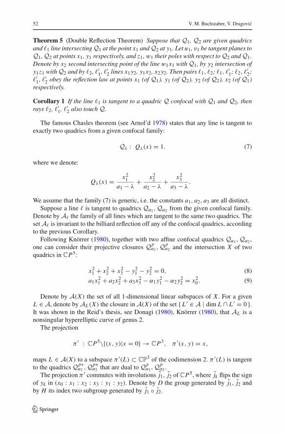
52 V. M. Buchstaber, V. Dragovic
Theorem 5 (Double Reflection Theorem) Suppose that Q1, Q2 are given quadricsand �1 line intersectingQ1 at the point x1 andQ2 at y1. Let u1, v1 be tangent planes toQ1,Q2 at points x1, y1 respectively, and z1,w1 their poles with respect toQ2 andQ1.Denote by x2 second intersecting point of the line w1x1 withQ1, by y2 intersection ofy1z1 withQ2 and by �2, �′
1, �′2 lines x1y2, y1x2, x2y2. Then pairs �1, �2; �1, �′
1; �2, �′2;
�′1, �
′2 obey the reflection law at points x1 (of Q1), y1 (of Q2), y2 (of Q2), x2 (of Q1)
respectively.
Corollary 1 If the line �1 is tangent to a quadric Q confocal with Q1 and Q2, thenrays �2, �′
1, �′2 also touch Q.
The famous Chasles theorem (see Arnol’d 1978) states that any line is tangent toexactly two quadrics from a given confocal family:
Qλ : Qλ(x) = 1. (7)
where we denote:
Qλ(x) = x21a1 − λ
+ x22a2 − λ
+ x23a3 − λ
.
We assume that the family (7) is generic, i.e. the constants a1, a2, a3 are all distinct.Suppose a line � is tangent to quadrics Qα1 ,Qα2 from the given confocal family.
Denote by A� the family of all lines which are tangent to the same two quadrics. ThesetA� is invariant to the billiard reflection off any of the confocal quadrics, accordingto the previous Corollary.
Following Knörrer (1980), together with two affine confocal quadrics Qα1 ,Qα2 ,one can consider their projective closures Qp
α1 ,Qpα2 and the intersection X of two
quadrics in CP5:
x21 + x22 + x23 − y21 − y22 = 0, (8)
a1x21 + a2x
22 + a3x
23 − α1y
21 − α2y
22 = x20 . (9)
Denote by A(X) the set of all 1-dimensional linear subspaces of X . For a givenL ∈ A, denote byAL(X) the closure inA(X) of the set { L ′ ∈ A | dim L ∩ L ′ = 0 }.It was shown in the Reid’s thesis, see Donagi (1980), Knörrer (1980), that AL is anonsingular hyperelliptic curve of genus 2.
The projection
π ′ : CP5\{(x, y)|x = 0} → CP3, π ′(x, y) = x,
maps L ∈ A(X) to a subspace π ′(L) ⊂ CP3 of the codimension 2. π ′(L) is tangent
to the quadrics Qp∗α1 ,Qp∗
α2 that are dual to Qpα1 ,Qp
α2 .The projection π ′ commutes with involutions j1, j2 ofCP5, where jk flips the sign
of yk in (x0 : x1 : x2 : x3 : y1 : y2). Denote by D the group generated by j1, j2 andby H its index two subgroup generated by j1 ◦ j2.
123
Two-Valued Groups, Kummer Varieties… 53
Thus, the space dual to π ′(L), denoted by π∗(L), is a line tangent to the quadricsQp
α1 ,Qpα2 .
Recall the notion of the generalized Cayley’s curve from Dragovic and Radnovic(2006, 2008).
Definition 3 The generalized Cayley curve C� is the variety of hyperplanes tangentto quadrics of a given confocal family in CP3 at the points of a given line �.
This curve is naturally embedded in the dual space CP3 ∗.
Proposition 5 The generalized Cayley curve inCP3, is a hyperelliptic curve of genus2. Its natural realization in CP3 ∗ is of degree 5:
y2 = (x − a1)(x − a2)(x − a3)(x − α1)(x − α2).
The natural involution τ� on the generalized Cayley’s curve C� maps to each otherthe tangent planes at the points of intersection of � with any quadric of the confocalfamily. Thus, the factor:
Y = C�/τ�, (10)
is naturally seen as the pencil of quadrics; thus an isomorphism is defined i2 : Y →CP1 and each point in Y corresponds to a quadric of the pencil.
(It was observed in Dragovic and Radnovic (2006) that this curve is isomorphic tothe Veselov-Moser isospectral curve.)
Now we are going to mention a connection obtained in Dragovic and Radnovic(2008), between generalized Cayley’s curve defined above and the curves (see theprevious Section) studied by Knörrer, Donagi, Reid. This connection traces out therelationship between billiard constructions and the algebraic structure of the corre-sponding Abelian varieties.
We can reinterpret the generalized Cayley’s curve C�, which is a family of tangenthyperplanes, as a set of lines from A� which intersect �. Namely, for almost everytangent hyperplane there is a unique line �′, obtained from � by the billiard reflection.Having this identification in mind, it is easy to prove the following
Corollary 2 There is a birational morphism between the generalized Cayley’s curveC� and the Reid-Donagi-Knörrer’s curve FL , with L = π∗−1(�), defined by
j : �′ �→ L ′, L ′ = π∗−1(�′),
where �′ is a line obtained from � by the billiard reflection off a confocal quadric.
Thus, there is a link between the dynamics of ellipsoidal billiards and algebraicstructure of certain Abelian varieties.
Denote by K the Kummer variety of A(X). Denote by K1 the Kummer variety ofthe Jacobian of the Cayley curve Jac(C�. Then, see Knörrer (1980), K1 = A(X)/G =K/H . Then the embedding i : C� → Jac(C�) induces an embedding i : Y → K1.
If we denote by m : K × K → (K )2 the structure of algebraic two-valued groupon the Kummer variety as defined above, then there is an induced two-valued group
123
54 V. M. Buchstaber, V. Dragovic
structure b on the Kummer variety K1:
K × K
p×p
m (K
)2
(p)2
K1 × K1b (
K1)2
,
where p is the projection induced by the projection p : A(X) → A(X)/H.
If we specialize the above morphisms to Y defined by the Eq. (10), we get thefollowing commutative diagram:
Y × K1i×id
i2×id
K1 × K1m (
K1)2
(id)2
CP1 × K1b (
K1)2
.
For a given λ ∈ CP1 and a line �1 ∈ K1, which is tangent to the both given confocalquadrics Qα1 and Qα2 , we have that
b(λ, �1) = (�2, �3) ∈ (K1)2.
Here �2, �3 are the two lines tangent to the both given confocal quadrics Qα1 and Qα2 ,which are obtained from �1 after the billiard reflection off the quadric Qλ.
8 Moduli of Semi-Stable Bundles and Two-Valued Group Structure onKummer Varieties
As we have mentioned before, historically first examples of 2-valued groups appearedin topological context in the study of the characteristic classes of vector bundles,see Buchstaber and Novikov (1971). There one-dimensional symplectic bundles overHP
n , and together with the canonical projection CP2n+1 → HPn , the associatedtwo-dimensional complex vector bundles overCP2n+1 with c1 = 0, were considered.
For a pair of such two-dimensional bundles,
ξ1, ξ2, c1(ξi ) = 0, i = 1, 2
its tensor productξ1 ⊗C ξ2
is a four-dimensional bundle, with the first two Potryagin classes p1(ξ1 ⊗C ξ2) andp2(ξ1 ⊗C ξ2). In Buchstaber and Novikov (1971), to the initial pair of bundles, a pairof virtual two-bundles, were associated according to the formula
123
Two-Valued Groups, Kummer Varieties… 55
Z2 − p1(ξ1 ⊗C ξ2)Z + p2(ξ1 ⊗C ξ2) = 0.
The solutions Z1,2 of the last quadratic equation play a role of the first Pontryaginclasses of two virtual two-bundles. The last quadratic equation defines a two-valuedgroup structure in x = p1(ξ1) and y = p1(ξ2), since p1(ξ1 ⊗C ξ2) = �1(x, y) andp2(ξ1 ⊗C ξ2) = �2(x, y), where �i are certain series.
In this Section, we are going to construct the two-valued group structure on theKummer variety, in the context of two-dimensional varieties, semi-stable in the senseof Mumford and Seshadri. The significance of the present situation, lies in the factthat obtained resulting two-bundles are not virtual - they are realized as a pair oftwo-bundles, semi-stable but not stable.
To get this, yet another interpretation of Kummer varieties, we are going back toNarasimhan and Ramanan (1969) Let X be a genus two curve. Following Mumfordand Seshadri, the notions of stable and semi-stable vector bundles of rank n and degreed have been introduced respectively. For a holomorphic nonzero vector bundle W onX one introduces a rational-valued function μ(W ) = degW/rankW . A vector bundleW is stable if for every proper subbundle V the condition
μ(V ) < μ(W )
is satisfied. Similarly, a bundle is semi-stable if in the last inequality the sign < isreplaced by ≤. Any semi-stable bundle W has a strictly decreasing filtration
W = W0 ⊃ W1 ⊃ · · · ⊃ Wn = {0}
such that Wi−1/Wi are stable and μ(Wi−1/Wi ) = μ(W ). Denote by GrW =⊕Wi−1/Wi . As Seshadri defined, two semi-stable bundlesW1 andW2 are S-equivalentifGrW1 ≈ GrW2; a normal, projective (n2+1)-dimensional variety of S-equivalenceclasses of semi-stable bundles of degree d and rank n denote U (n, d).
Following Narasimhan and Ramanan (1969), for U (2, 0), denote by S its three-dimensional sub-variety of bundles with trivial determinant. The non-stable bundlesin S are of the form
j ⊕ j−1,
with j a line bundle of degree 0. The Kummer surface K associated to the Jacobianof X is isomorphic to the set of all non-stable bundles in S.
Now,wedefine a structure of two-valued group on K . It is an important developmentof the Example 4 from Sect. 2. Denote a, b ∈ K , where
a = j ⊕ j−1, b = l ⊕ l−1,
where j, l are line bundles on X of degree 0. Then:
a �s b := ( j ⊗ l ⊕ j−1 ⊗ l−1, j ⊗ l−1 ⊕ j−1 ⊗ l). (11)
123
56 V. M. Buchstaber, V. Dragovic
Proposition 6 The operation
�s : K × K −→ (K )2
determined by the relation (11) defines a two-valued group structure on K .
Acknowledgements The authors would like to thank the reviewers for their helpful remarks. The researchof one of the authors (V. D.) was partially supported by the Serbian Ministry of Education, Science, andTechnological Development, Project 174020 Geometry and Topology of Manifolds, Classical Mechanics,and Integrable Dynamical Systems.
References
Arnol’d, V.: Mathematical methods of classical mechanics. Springer, New York (1978)Audin, M.: Spinning tops. An introduction to integrable systems, Cambridge studies in advanced mathe-
matics 51 (1999)Audin, M.: Courbes algebriques et syst‘emes integrables: geodesiques des quadriques. Expo. Math. 12,
193–226 (1994)Baker, H.F.: On the hyperelliptic sigma functions, Am. J. Math. 301–384 (1898)Buchstaber, V.M., Novikov, S.P.: Formal groups, power systems and Adams operators. Mat. Sb. (N. S)
84(126), 81–118 (1971). (in Russian)Buchstaber, V.M., Rees, E.G.: Multivalued groups, their representations and Hopf algebras. Transform.
Groups 2, 325–249 (1997)Buchstaber, V.M., Veselov, A.P.: Integrable correspondences and algebraic representations of multivalued
groups, Internat. Math. Res. Notices, 381–400 (1996)Buchstaber, V.M.: Functional equations that are associated with addition theorems for elliptic functions, and
two valued groups, Uspekhi Math. Nauk 45 (1990) No 3 (273) 185–186 (Russian) English translation.Russian Math. Surveys 45(3), 213–215 (1990)
Buchstaber, V.M.: n-Valued groups: theory and applications. Moscow Math. J. 6, 57–84 (2006)Buchstaber, V.M.: Polynomial dynamical systems and the Korteweg-de Vries equation. Proc. Steklov Inst.
Math. 294, 176–200 (2016)Buchstaber, V.M., Mikhailov, A.V.: Infinite-dimensional lie algebras determined by the space of symmetric
squares of hyperelliptic curves. Funct. Anal. Appl. 51(1), 4–27 (2017)Buchstaber, V.M., Enolskii, V.Z., Leikin, D.V.: Kleinian functions, hyperelliptic Jacobians and applications.,
Reviews in Mathematics and Math. Physics, Krichever, I.M., Novikov, S.P. Editors, v. 10, part 2,Gordon and Breach, London, 3–120 (1997)
Buchstaber,V.M., Enolskii,V.Z., Leikin,D.V.:Multi-dimensional sigma-functions. arXiv:1208.0990 [math-ph] (2012)
Buchstaber, V.M., Leykin, D.V.: Addition laws on Jacobian varieties of plane algebraic curves. Proc. SteklovMath. Inst. 251(4), 49–120 (2005)
Buchstaber,V.M., Rees, E.G.: TheGelfandmap and symmetric products. SelectaMath. (N.S.) 8(4), 523–535(2002)
Darboux, G.: Principes de géométrie analytique, p. 519. Gauthier-Villars, Paris (1917)Donagi, R.: Group law on the intersection of two quadrics Ann. Sc. Norm. Sup. Pisa, 217–239 (1980)Dragovic, V.: Poncelet-Darboux curves, their complete decomposition andMarden theorem. Internat.Math.
Res. Notes 2011, 3502–3523 (2011)Dragovic, V.: Multi-valued hyperelliptic continous fractions of generalized Halphen type. Internat. Math.
Res. Notices 2009, 1891–1932 (2009)Dragovic, V.: Generalization and Geometrization of the Kowalevski top. Comm.Math. Phys. 298(1), 37–64
(2010)Dragovic, V., Kukic, K.: Discriminantly separable polynomials and quad-graphs. J. Geom. Mech. 6(3),
319–333 (2014)Dragovic, V., Kukic, K.: Systems of the Kowalevski type and discriminantly separable polynomials. Regul.
Chaotic Dyn. 19(2), 162–184 (2014)
123
Two-Valued Groups, Kummer Varieties… 57
Dragovic, V., Kukic, K.: The Sokolov case, integrable Kirchhoff elasticae, and genus 2 theta-functions viadiscriminantly separable polynomials. Proc. Steklov Math. Inst. 286, 224–239 (2014)
Dragovic, V., Radnovic, M.: Geometry of integrable billiards and pencils of quadrics. J. Math. Pures Appl.85, 758–790 (2006)
Dragovic, V., Radnovic, M.: Hyperelliptic Jacobians as Billiard Algebra of Pencils of Quadrics: BeyondPoncelet Porisms. Adv. Math. 219, 1577–1607 (2008)
Dragovic, V., Radnovic, M.: Poncelet porisms and beyond: integrable billiards, hyperelliptic Jacobians andpencils of quadrics, Frontiers in Mathematics, Birkhauser/Springer, 294, ISBN 978-3-0348-0014-3(2011)
Dragovic, V., Radnovic,M.: Bicentennial of the Great Poncelet Theorem. Bull. Am.Math. Soc. 51, 373–445(2014)
Dragovic, V., Radnovic, M.: Pseudo-integrable billiards and arithemetic dynamics. J. Modern Dyn. 8(1),109–132 (2014)
Dragovic, V., Radnovic, M.: Periods of pseudo-integrable billiards. Arnold Math. J. 1(1), 69–73 (2015).https://doi.org/10.1007/s40598-014-0004-0
Dragovic, V., Radnovic, M.: Pseudo-integrable billiards and double reflection nets. Russian Math. Surv.70(1), 3–34 (2015). https://doi.org/10.4213/rm9648
Dragovic, V., Gajic, B.: Some recent generalizations of the classical rigid body systems. Arnold Math. J.2(4), 511–578 (2016)
Dubrovin, B.A., Novikov, S.P.: A periodic problem for the Korteweg-de Vries and Sturm-Liouville equa-tions. Their connection with algebraic geometry (Russian) Dokl. Akad. Nauk SSSR 219 (1974),531-534, English translation: Soviet Math. Dokl. 15 (1974), no. 6, 1597–1601 (1975)
Gelfand, I.M., Kapranov, M.M., Zelevinsky, A.V.: Discriminants, resultants and multidimensional detemi-nants. Birhauser, Boston (1994)
Golubev,V.V.: Lectures on the integration ofmotion of a heavy rigid body around afixed point,Gostechizdat,Moscow, 1953 [in Russian] Israel program for scintific literature, English translation (1960)
Griffiths, Ph, Harris, J.: Principles of Algebraic Geometry. Wiley Classics library edition (1994)Knörrer, H.: Geodesics on the ellipsoid. Invent. Math. 59, 119–143 (1980)Kowalevski, S.: Sur la probleme de la rotation d’un corps solide autour d’un point fixe. Acta Math. 12,
177–232 (1889)Moser, J., Veselov, A.: Discrete versions of some classical integrable systems and factorization of matrix
polynomials. Commun. Math. Phys. 139(2), 217–243 (1991)Narasimhan, M., Ramanan, S.: Moduli of vector bundles on compact Riemann surfaces. Ann. Math. 2(89),
14–51 (1969)Tyurin, A.N.: On intersection of quadrics. Russian Math. Surv. 30, 51–105 (1975)Veselov, A.: Growth and integrability in the dynamics of mappings. Commun. Math. Phys. 145, 181–193
(1992)
123